stress distribution in a rectangular plate having two...

598

Stress Distribution in a Rectangular Plate having two Opposing Edges Sheared in Opposite Directions.

By C. E. Inglis, M.A., M.I.C.E.

(Communicated by Prof. E. G. Coker, F.R.S. Received February 8, 1923.)

The type of deformation under investigation is indicated by fig. 1.A rectangular plate ABCD is deformed into the shape A'B'C'D'.The two opposing edges AB, CD are shifted horizontally without alteration

of length into the position A'B', C'D', the other boundaries AD, BC being kept free from external stress.

In a paper which appeared in the ‘ Proc. Royal Society/ December 28, 1911, Prof. E. G. Coker investigated this same type of deformation using optical methods to determine the distribution of stress along the centre line OX. He found that if the plate was square the shear stress along OX

was distributed in a manner which was approximately parabolic. As the ratio of AD to AB decreased the curve of distribution first of all became flat- topped, and for yet smaller ratios two distinct humps made their appearance.

In the f Proc. Royal Society/June, 1911, Andrade presents an analytical treatment of this problem. The results of his analysis did not agree very satisfactorily with his experiments, and the author himself discusses the reliability of the analytical method adopted.

The following discussion takes a different line, and the distributions of stress obtained are apparently in close agreement with those experimentally determined by Prof. Coker.

In the 'Phil. Trans./ 1903, A 334, Prof. Filon discusses the somewhat similar case of a beam of rectangular section sheared by forces applied to the top and bottom surfaces. In this case the double peaks in the shear stress distribution are very pronounced.

General Method.

The problem stated above is dealt with by superposing two cases :—Case (1). The plate ABCD is considered to have its edges AB, CD absolutely

fixed, the other edges AD, BC being subjected to shear stress uniformly distributed along these boundaries.

VI

a I a'

O' D C'CFig. 1.

on July 8, 2018http://rspa.royalsocietypublishing.org/Downloaded from

http://rspa.royalsocietypublishing.org/

Stress Distribution in a Rectangular Plate. 599

Case (2). The plate ABCD is subjected to shear stress uniformly distributed along all four edges.

By combining these two cases the shear stress on the edges AD, BC can be eliminated and the type of deformation which results is that represented by fig. 1.

Notation .

The axes of co-ordinates selected are shown on fig. 1. The origin is at the centre of AD and OA OD are unit length. The three stress components defining the stress at a point are denoted by R*, Ry, S. The shifts of a point in direction OX OY are u and v. The modulus of elasticity is E and Poisson's ratio is 1/m.

Assuming that the plate is thin* and that in consequence the distribution of stress is two dimensional, Rx, Ry and S can be derived from a single stress function Y which satisfies the equation y 4 Y = 0, R*, Ry and S having the- values 02Y /dy2, 32Y /dx2, and —d2V/dxdy respectively.

Consider the following solution :—

V = — — xe~nx sin ny,

giving R* = AnxeTnx sin ny,

Ry = A (2—nx) e~nx sin ny ,

S — A (1—nx) e~nx cos ny.

I t follows from the relations

T7’ 3^ _ T) 1 T>Jli X -- VXx -Tty E ^ = Ry—— E;ox m cy m

that A P——̂ i + af] e n* sin ny, wE Lra+1 n J

v ra -f l * T 2m— — A x ---------mb L m +1 cos ny.

Along the boundary AD, S = A cos ny, and by putting ?i = 7r/2, 37t/2,. 57t/ 2, etc., and giving the corresponding constants A the values 4/7r, 4/37t,. 4/57T, etc., a uniform shear stress distribution having unit value can be built up along the edge AD.

In the arithmetical computation which follows, ten harmonic components

* If mean stresses and mean displacements are considered, the assumption that the- plate is very thin is not necessary.



600 C. E. Inglis.

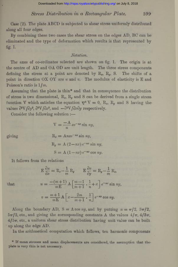
are taken and the degree of approximation to a uniform distribution of shear stress along AD obtained by superposing these ten components is made apparent by fig. 2.

Along AD, the value of R* is zero.Owing to the destructive influence of the factor e~nx the stresses generated

at the boundary x = 0 die out rapidly as x increases, and if the edge BC

Approximation to unit shear stress along AD produced by ten harmonic components.

coresponds to x = 4, i.e., if AB : AD = 2:1, this edge is practically not affected by any of the stress components applied along the boundary AD.

Along the top and bottom edges y = + 1 for the values of n selected, the value of v is zero throughout, but unfortunately the distribution of u is neither zero nor constant. Superposing the ten distributions of u corresponding to the ten harmonic components of S, and taking m to have the value of 10/3, the distribution of m/m.+ l Eu, i.e., 10/13 Eu along the top boundary is set forth numerically in Table I and illustrated by fig. 3.

Eor further reference the above distributions of stress and strain will be termed “ A ” distributions, and the shift along the top edge will be denoted by u±.

For a reason which will transpire later it is necessary to harmonically analyse the distribution of uA represented in fig. 3 along the boundary, i.e., between the limits x = 0 and x = 4.



Stress Distribution in Rectangular Plate.601

Taking eleven components, a close approximation is obtained by putting

Ewa = T0-2 0033 + 0-24918 cos— + 008196 cos13 7T3 L 4

+ 0-02591 cos + 0'00652 cos4 4

+ 0-00167 cos —0'00104 cos ^7rJ

2n t x

—0-00132 cos

— 0’00171 cos

477T2;

97HC~ T '

■0-00192 cos

•0-00203 cos

48 irx~

107raf|4~ J

The degree of accuracy obtained by this approximation is shown numerically in Table I and graphically in fig. 3.

The full line curve in the accurate distribution of —10/13 E along AB.The dotted line curve is the harmonic approximation, and is only distin

guishable from the true curve in the immediate neighbourhood of the corner A.

Next consider a solution of y 4Y = 0 in the form

Y = ----- sin nxn3'(m— 1

giving

Ex = B sin nx I (n sinh n■['

( — y cosh n —n sinh nj sinh ny + ny cosh n cosh ny ,

3/?i + 1 cog ̂^ Uy__Uy C08j1 n cosj1 Uy~̂m + 1

By = B sin nx cosh ?i— n sinh nj sinh ny + ny cosh n cosh ny\^

S = B cos nx cos^ n —n sinh nj cosh ny + ny cosh n sinh ny J,

ra + l-D f/3m — 1 cosh , \ . , , . 1u = —— B cos nx —----- —----- smh nj sinh ny + y cosh n cosh ny J ,

v = B sin nx [y cosh n sinh ny— sinh n cosh ny\

These expressions will be referred to as “ B ” distributions of stress and strain.

Taking AB = 4 and AD = 2 as before, if n is any whole number multiple of 7t/4 , B* is zero at both boundaries AD and BC.

Along the edges AB, CD where y = ± 1, v is zero throughout.The values of uB along these same boundaries are harmonic functions of x



.abour involved. I t will be seen that the error, such as it is, is localised at a

s CD 51

'P

"

CO

CD

^CD

sr

sr d3 CD

3 P w E H+s

GO*

3C+ P" CD

CT* CD̂ cT CD P

PT1 CD O cy p *-s p o S'

p o cd p l-S p CD o p p * CD P^

CD

O

*.1

s I

&

s

^

&C—

i. g e£ CD GO c* P*1

CD CD * c-r P P g P- P B CD 5* $

p- t—<• as CD CD P CD CD a" CD 3 CD CD P C+" D- CD O P •-i <

O P

* CD

^

§

p S

§of

r g

4

I. &

i+°

& a

3. g

o' ^

p

&

CD o B ip o p CD P S' CD P P cr CD

£L ^

§

g g,c-K S"

^CD

P CD

CD

0_

< P

aqS'

sE-

»S

* o

CD

t-h.

p-

p•

t—<

p t—■ • aq S' I-S s

p GO

CO

E GO P o p CD c+- PP CD

CD '

O

- 3

p

pp

* §

% &

M

B3

°Qhp 3

oGO CD

^

I "

P-

O

^ 5'

S 9v

o o

fT 0)

o £

® a rr

a?

D O

O

C C&

(fi

Note: Where not other

o

n n a5

£I

8 5

» -

o-3

% e.

§

?

§

»*

o

° -

r

o § o

sro0

so m

* *5

3 >>

6) r-

, ©

z °

oB

3 D

<0

0- -o

> rr

—

CP

J

:

-n“•

si

g w

l—"

c*

< £- g■H

w to

p- >

H>-

iHw top

iH>-

to(H

^|v

- i^

|w

*.|w

-0-52755 -0-57399 - 0 *51730 -0*43968 -0-35975 -0*28629 -0*22291 -0*17074 -0*12898 - 0 *09633 -0-07131 - 0 *05238 -0*03824 -0*02774 - 0 *02004 -0-01441 - 0 *01032

Value of 10/13 Eu obtained by taking ten

“ A ” Functions.

+ 0-57540 0 *56554 0 *52082 0 *44008 0 *35754 0 *28787 0 22316 0 *16930 0 *13008 0 -09663 0 *07018 0 *05323 0 -03853 0 *02672 0 *02073 0 *01458 0 -01041

Harmonicapproximations.

+ 0-04785 -0*00845 + 0 *00352 + 0*00040 -0-00221 + 0*00158 + 0*00025 - 0 '00144 + 0-00110 + 0 -00030 -0*00113 + 0*00085 + 0 -00029 -0*00102 + 0 *00069 + 0*00017 + 0-00009

Residual value! 10/13 E«.

8.

H p CD- hH 1 cl^

I

£ g

P t+3

CD

ct-

M

P bO X I—1 hj p" S'

CD O togiven for 10 E/13 .

on

July

8, 2

018

http

://rs

pa.r

oyal

soci

etyp

ublis

hing

.org

/D

ownl

oade

d fr

om


Stress Distribution in a Rectangular Plate.603

corner and cannot appreciably affect the distribution of stress at the comparatively distant centre line which is the main point of this investigation.

The introduction of these eleven “ B ” components while effectively achieving zero shift along the top and bottom edges does not build up any appreciable shear stress along the edge BC,* and it has been arranged that is zero both along BC and AD. Unfortunately the shear stress they introduce along the edge AD cannot be dismissed thus lightly.

Addition bo snear s tress 3long AD consequent on com bining the F irs t and second “8 “ distributionswith the. A* distribution given by S - — cos

F; rst " 6" di stri bu tion oP shear stress along AD.

Second 8 distribution of sh ear s tr e s s a long A D .

Fig. 4-

The value of this “ B ” shear stress distribution along AD is graphically represented by the middle curve appearing on fig. 4. I t will be seen that

* The insignificance of the shear stress along the edge BC is not a mere happy numerical accident, but it admits of a physical explanation. The <c B ” distribution of stress and strain employed is periodic in a length 8. Consider the 4 x 2 plate as the left half of an 8 x 2 plate. For the middle region of this 8 x 2 plate the top and bottom edges are almost rigidly fixed, since v = 0 and u is nearly zero for an appreciable length. This fixing will to a considerable extent shield the plate in this middle region from the action of stresses applied at the ends, and consequently for the 4 x 2 plate there is reason to anticipate that along the edge BC the distribution of shear stress will be insignificant.

VOI. CI11.— A. 2 K



604 C. E. Inglis.

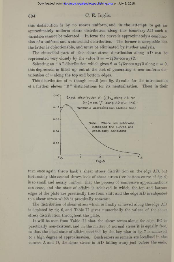
this distribution is by no means uniform, and in the attempt to get an approximately uniform shear distribution along this boundary AD such a variation cannot be tolerated. In form the curve is approximately a combination of a uniform and a sinusoidal distribution. The former is acceptable but the latter is objectionable, and must be eliminated by further analysis.

The sinusoidal part of this shear stress distribution along AD can be represented very closely by the value S = — 2/37T cos7n//2.

Selecting an “ A ” distribution which gives S = 2/37tcos7T2//2 along x = 0, this depression is filled up but at the cost of generating a non-uniform distribution of u along the top and bottom edges. •

This distribution of u though small (see fig. 5) calls for the introduction of a further eleven “ B ” distributions for its neutralisation. These in their

Exact d is tr ib u tio n of - EuA along A B for

5 « | tt cos along A D (fu ll line)

x. H arm onic approxim at*on (d o tte d line,)

N ote- Where not otherwise ind ica ted the curves are

v p ractica lly coincident.

Fig..-5.

turn once again throw back a shear stress distribution on the edge AD, but fortunately this second throw-back of shear stress (see bottom curve of fig. 4) is so small and nearly uniform that the process of successive approximations can cease, and the state of affairs is achieved in which the top and bottom edges of the plate are practically free from shift and the edge AD is subjected to a shear stress which is practically constant.

The distribution of shear stress which is finally achieved along the edge AD is depicted by fig. 6, and Table II gives numerically the values of the shear stress distribution throughout the plate.

It will be seen from Table II that the shear stress along the edge BC is practically non-existent, and in the matter of normal stress it is equally free, so that the ideal state of affairs specified by the key plan in fig. 7 is achieved to a high degree of approximation. Such errors as remain are localised in the corners A and D, the shear stress in AD falling away just before the ends,



Stress Distribution in Rectangular Plate. 605

see fig. 6, and the horizontal shifts in the top and bottom edges not being perfectly neutralised right up to the corners, see figs. 3 and 5. These

D is trib u tio n o f shear stress fin a lly applied along ed g e A D M ean V a lu e 1-43 approxim ately.

0*6 -

0 -4 -

Table II.—Shear Stress Distribution. 2 x 1 Plate.Fixed along edges y = +1, and carrying an approximately uniform shear

stress distributed along the edge x = 0.

0. 4. h , Valuesof y.

b 0 1 *39716 1 -42571 1 -46406 1 -41755 0 -43122i 0 -82654 0 -79966 0 *70643 0 *51703 0 *46944

0 *39920 0 -37819 0 -32414 0 -29542 0 -448091 0 -15204 0 -14910 0-15327 0 -19969 0 *29464

1 0 -03236 0-04111 0 -07253 0 *13222 0-18012H -0*01552 - 0 -00362 0 -03131 0 *08258 0-14111

H li - 0 -02822 -0-01790 0 -01177 0 -05086 0 08092•s is - 0 -02679 -0-01906 0 -00319 0 -03058 0 -03668S 2 - 0 -02160 - 0 -01585 -0-00088 0 *01680 0 -036714 2± -0-01470 -0-01146 - 0 -00175 0 00956 0 -01778

£ 2 i - 0 -00941 -0-00748 -0-00132 0 00558 - 0 000422S - 0 -00570 - 0 -00440 -0*00103 0 -00240 0 -011203 - 0 *00233 -0-00176 -0-00031 0 *00121 0 -0044034 0 -00075 0 -00080 0 00085 0 -00072 -0-007823* 0 -00398 0 -00350 0 -00184 -0*00066 0 004023f 0 -00771 0 -00685 0 00419 - 0 -00075 - 0 005034 0 -01209 0 -01089 0 -00753 0 -00085 -0-02289

departures from the ideal introduce an element of uncertainty concerning the stresses in the corners but they can have no appreciable effect on the distribution of shear stress along the centre line.

2 n 2



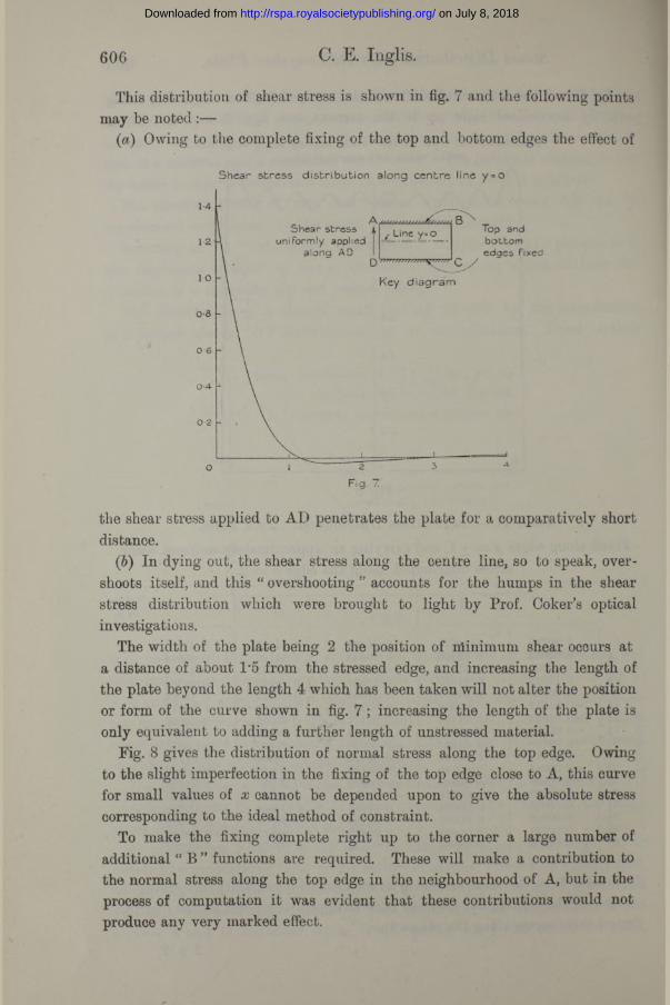
This distribution of shear stress is shown in fig. 7 and the following points may be noted

(a) Owing to the complete fixing of the top and bottom edges the effect of

606 C. E. Inglis.

S hea r s tre s s d is t r ib u t io n a lo n g c e n tre lin e y = o

S h e a r s tre s s un ifo rm ly applied

along AD

Top and b o t to m edges fix e d

^ L ine y= 0

Key d ia g ra i

the shear stress applied to AD penetrates the plate for a comparatively short distance.

(b) In dying out, the shear stress along the centre line, so to speak, overshoots itself, and this “ overshooting ” accounts for the humps in the shear stress distribution which were brought to light by Prof. Coker’s optical investigations.

The width of the plate being 2 the position of nlinimum shear occurs at a distance of about 1*5 from the stressed edge, and increasing the length of the plate beyond the length 4 which has been taken will not alter the position or form of the curve shown in fig. 7 ; increasing the length of the plate is only equivalent to adding a further length of unstressed material.

Fig. 8 gives the distribution of normal stress along the top edge. Owing to the slight imperfection in the fixing of the top edge close to A, this curve for small values of x cannot be depended upon to give the absolute stress corresponding to the ideal method of constraint.

To make the fixing complete right up to the corner a large number of additional “ B ” functions are required. These will make a contribution to the normal stress along the top edge in the neighbourhood of A, but in the process of computation it was evident that these contributions would not produce any very marked effect.



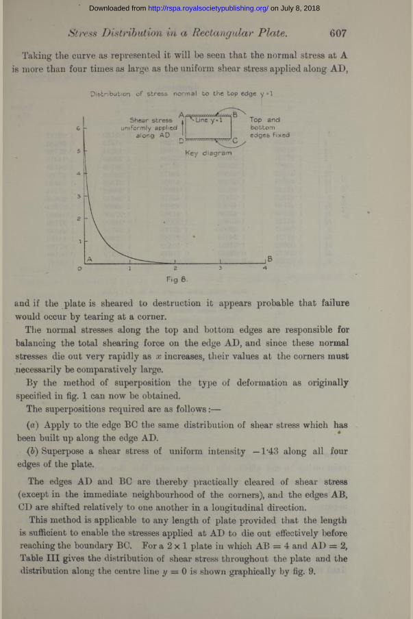
Taking the curve as represented it will be seen that the normal stress at A is more than four times as large as the uniform shear stress applied along AD,

Stress Distribution in Rectangular Plate. 607

D is tr ib u t io n o f s tre ss n o rm a l to the top edge y = l

Top and b o tto m edges Fixed

Shear s tre ss u n ifo rm ly applied

a long AD

Line y »1

Key d ia g ra m

and if the plate is sheared to destruction it appears probable that failure would occur by tearing at a corner.

The normal stresses along the top and bottom edges are responsible for balancing the total shearing force on the edge AD, and since these normal stresses die out very rapidly as x increases, their values at the corners must necessarily be comparatively large.

By the method of superposition the type of deformation as originally specified in fig. 1 can now be obtained.

The superpositions required are as follows:—(a) Apply to the edge BC the same distribution of shear stress which has

been built up along the edge AD.(b) Superpose a shear stress of uniform intensity —1*43 along all four

edges of the plate.

The edges AD and BC are thereby practically cleared of shear stress (except in the immediate neighbourhood of the corners), and the edges AB, CD are shifted relatively to one another in a longitudinal direction.

This method is applicable to any length of plate provided that the length is sufficient to enable the stresses applied at AD to die out effectively before reaching the boundary BC. For a 2 x 1 plate in which AB = 4 and AD = 2, Table II I gives the distribution of shear stress throughout the plate and the distribution along the centre line y == 0 is shown graphically by fig. 9.



608 C. E. Inglis.

Top and bottom edges having a constant longitudinal shift in oppositedirections.

Table IIL^—Shear Stress Distribution. 2 x 1 Plate.

0 . *. 4. b . V alueso f ? .

0 0-02075 - 0 00660 -0-04159 0 -01160 1 -021674 0 -59575 0 *62349 0 -71938 0 -91372 0 *96589i 1 02682 1 04831 1 -10402 1 -13524 0 *97789

1-27721 1 -28010 1 -27588 1*22959 1 *14318l* 1-39897 1 -39065 1 -35778 1 -29706 1 -24548

. 14 1 -45122 1 *43802 1 -39972 1 -34502 1 -27769» H 1 -46763 1 -45538 1 -41955 1 -37356 1*34950O I f 1 -47149 1 -46052 1*42856 1 -38986 1 -37554S 2 1 -47320 1 *46170 1 -43176 1 -39640 1 -35658

5 24 1 -47149 1-46052 1 -42856 1 *38986 1 *37554£ 24 1 -46763 1 -45538 1 -41955 1*37356 1 -34950

2* 1 -45122 1 ‘43802 1 *39972 1*34502 1 -277693 1-39897 1 *39065 1 35778 1-29706 1 -2454834 1 -27721 1*28010 1*27588 1 ‘22959 1 *1431834 1 -02682 1 -04831 1 *10402 1*13524 0 *977893f 0 -59575 0 *62349 0 71938 0 *91372 0 *965894 0 -02075 - 0 -00660 - 0 -04159 0-01160 1 -02167

Shear s tress along c e n tre lin e fo r 2 * 1 p la te

P la te has i ts ends fre e and i ts top andb o tto m edges sheared in opposite d irections

u shif t

fre e /

-*---- u shiftKey d ia g ra m

Owing to the comparatively short length of the plate the humps which exist owing to end effects run together, and this fact accounts for its flat topped appearance. In fig. 10 which gives the centre line shear stress for a 4 x 1 plate, the humps due to the end effects do not superpose and are apparent in the resulting distribution. Any further increase in the length of the plate is merely equivalent to introducing a central length subjected to a uniform shear stress, and the distribution of stress in the end regions remains the same as in the 4 x 1 plate.

Table II indicates that in the case of a plate with top and bottom edges fixed the shear stresses applied to the edge x = 0 have practically subsided as



Stress Distribution in a Rectangular Plate. 609

soon as the distance x = 2 is reached, and this statement is true for the other stress and strain components.

This being the case, the method of superposition adopted for the 2 x 1 plate

Shear s tress along c e n tre line fo r 4 * 1 Plate

P late has its ends free and its top andb o tto m edges sheared in opposite d ire c tio n s

u s h if t — *-

End 'J0-8 - h fre e

— • u s h if t Key d iagram

can again be put into operation to determine the distribution of shear along the centre line when a square plate has two of its opposing edges sheared in opposite directions.

Fig. 11 gives the shear stress so determined, and it will be noted that in this case the distribution is almost purely parabolic.

S hear s tre ss along ce n tre line fo ra square Plate

P la te has its ends free and its top and b o tto m edges sheared in opposite d ire c tio n s

u s h i f t ------ ►

-----u s h iftKey diagram

A comparison of these curves with those appearing in Prof. Coker’s paper referred to above, indicate that the results obtained by experiment and analysis are in close agreement, and such discrepancies as do occur may be accounted for by the fact that in these computations m has been taken as 10/3, whereas the optical experiments were performed on a material which had a value of m which was probably about 2*5.



610 H. E. Armstrong.

The above analysis has involved a very considerable amount of arithmetical calculation, only a small part of which appears in this paper. For the perseverance and accuracy with which this arithmetical work has been performed the main credit must be given to Mr. L. Patrick, B.A., Scholar of Queens’ College, Cambridge. Valuable assistance was also rendered by Mr. H. Quinney, a member of the teaching staff of the Engineering Laboratory, Cambridge.

The Origin o f Osmotic Effects. IV .— Hydronodynamic Change inAqueous Solutions.

By H enry E. A rm strong , F.R.S.

(Received March 22, 1923.)

From 1885 onwards, in communications to this Society and elsewhere, I have advocated an electrolytic explanation of chemical change, reciprocally a chemical explanation of electrolysis, in which no assumption is made beyond the ordinary canons of chemical belief. I have reason to think that, even now, my conception is in no way understood. I also can but recognise that I have not yet presented my full case.

The following statement is an attempt to show that a simple explanation may be given of the operations involved in the dissolution of “ salts ” in water, of the same mathematical form as the ionic dissociation hypothesis, accounting equally well for electrical and osmotic peculiarities, which has the advantage that it is in harmony with general chemical experience. Although in most part but a repetition of arguments already advanced, the statement is more comprehensive and definite than any previous attem pt; the consequences, particularly with respect to water, may prove to be not without application in other fields of inquiry.

Much of the difficulty, in any theoretical advance, is due to the force of prejudice and of dictated belief. The great obstacle, apparently, in arriving at an acceptable solution of the problem of chemical change (including electrolysis) has been the constant association of the symbol OH2 with “ water ” and the disregard of the determining part played by “ water ” ; “ water,” moreover, has an undeserved reputation for “ neutrality.” Actually, the symbol is only representative of the molecule in dry steam. The term water should be confined to the liquid. To give emphasis to this contention, I



stress distribution in a rectangular plate having two...

Documents