stream response to stormwater management best management

Stream Response To Stormwater Management Best Management Practices

In Maryland

Final Deliverable U. S. Environmental Protection Agency

Section 319(h) , Clean Water Act July, 2000

Deborah J. Cappuccitti William E. Page MARYLAND DEPARTMENT OF THE ENVIRONMENT Water Management Administration •••• Nonpoint Source Program 1800 Washington Boulevard • Baltimore, Maryland 21230(410) 537-3543 • http:// www.mde.state.md.us

Page LIST OF FIGURES ii LIST OF TABLES ii ACKNOWLEDGEMENTS iii ABSTRACT iv INTRODUCTION 1 HSPF MODEL DEVELOPMENT 2 Model Input Model Calibration HSPF and TR-20 MODELS 5 STORMWATER MANAGEMENT SCENARIOS 10

Scenario Development Evaluation of Scenarios CHANNEL STABILITY ANALYSIS 16 GUIDELINES FOR EVALUATING STORMWATER MANAGEMENT DESIGNS FOR STREAM CHANNEL PROTECTION 21 Stream Channel Geomorphic Assessment Stormwater Management Modeling CONCLUSION 22 REFERENCES 23 Appendix A: Hydraulic Function Tables Appendix B: HSPF Model Calibration Appendix C: Sensitivity Analysis Appendix D: Stormwater Management Scenarios Appendix E: Channel Stability Analysis

Stream Response to Stormwater Best Management Practices in Maryland

iii

LIST OF FIGURES Page

Figure 1: Benson Branch HSPF Segmentation 2 Figure 2: HSPF Calibration, Reach 1, Below Pond 1 4 Figure 3: HSPF – TR20 Comparison at Selected Rainfall Events 7 Figure 4: Stormwater Management Scenarios 13 Figure 5: Channel Stability Analysis, Pond 2 20 Figure 6: Channel Cross-section, Pond 2 20 Figure 7: Channel Stability Analysis, Pond 1 21 Figure 8: Channel Cross-section, Pond 1 21

LIST OF TABLES Table 1: Land Use by HSPF Segment for the Benson Branch Watershed 3 Table 2: Stage – Discharge – Shear Stress – Shear Stress Ratio 17


iv

ACKNOWLEDGEMENTS

This project was made possible through funding provided by the U.S. Environmental Protection Agency (U.S. EPA), under the Section 319 Nonpoint Source Program. This is a cooperative effort between the Maryland Department of the Environment’s Water Management Administration (WMA) and Technical Assistance and Regulatory Services Administration (TARSA). Tom Tapley, Wayne Jenkins, Angelica Gutierrez and Christine Shannon (TARSA) provided valuable assistance during project development and watershed modeling activities. William Page and Melissa Frank (WMA) also contributed to the modeling component of this project. We would also like to remember representatives from local governments for their assistance in providing information on stormwater management practices in their respective jurisdictions. These include Al Wirth (Baltimore County), Richard Brush (Montgomery County), Steve Sharar and Joe Kiddwell (Howard County), and Geoffrey Schoming (Howard County Soil Conservation District). In addition, the University of Maryland Agricultural Experiment Station in Clarksville allowed access to their property for rain data collection. Several members from WMA’s Nonpoint Source Program have participated in field work and provided technical assistance during all project phases. Thanks to Ken Pensyl, Brian Clevenger, Jim Tracy, Fred Jones, Ray Bahr, Steve Aust, Stew Comstock, Jim Fritz, Rick Trickett and Rebecca Winer. A special thank you is extended to Etta Lyles (MDE) for her very helpful and cheerful assistance in locating a large number of research documents. While the combined efforts from these people have been instrumental in the completion of this project, many people continue to provide support and inspire ideas to further the understanding gained herein. Thank you to all who continue in these efforts.


v

ABSTRACT

The primary objective of this report is to evaluate stormwater management strategies and

determine their effectiveness for protecting receiving stream channels. This was done by developing a watershed model of the Benson Branch watershed, in Howard County, Maryland. The data used for model development were collected in the field between 1996 and 1998, and reported in MDE, 1999. Results of the stormwater management modeling indicate that the channel protection volume (Cpv), (MDE, 2000) and the Distributed Runoff Control (DRC) methods (MacRae, 1993 and Ontario Ministry of the Environment, 1999) provide a similar level of management for the ponds simulated in this watershed. The highest level of control for both practices is focused on flows in the mid-bankfull range.

An evaluation of stream channel thresholds is provided to more completely analyze stormwater management strategies. A release of stormwater runoff below the stable channel threshold results in minimal impact on the stream channel. Using the stability analysis, the Cpv and DRC designs could protect the streams monitored in this study for storms less than 2.0” of rain, generally falling over a 24 hour period. Given that streams are highly variable with respect to hydrology and morphological stability thresholds, a site specific stream morphology study will improve efforts in evaluating the effectiveness of management strategies for stream channel protection.

Guidelines for evaluating stormwater management designs for stream channel protection are provided herein. The guidelines focus on evaluating receiving stream geomorphology and identification of stability thresholds. The results and implications found in this study pertain to the Benson Branch watershed in Howard County, Maryland. Using the guidelines to evaluate other streams in Maryland will expand the data set so that implications of these results may be applied on a broader scale.


INTRODUCTION

Maryland’s current stormwater management program was developed during the early 1980’s when flood control was the primary issue concerning urban runoff management. Prevailing experience had indicated that when flooding, caused by increases in runoff volume from new development could be controlled then the quality of receiving streams could be sustained. Consequently, the design criteria for the original Code of Maryland Regulations (COMAR) regulating stormwater runoff was to manage the release of peak flows for the 2 and 10 year design storms so that pre-development peak flows would not be exceeded.

After many years of experience on stormwater management implementation across Maryland, MDE has found that management of peak flows for the 2 and 10 year storms does not provide sufficient stream channel erosion protection from the increased runoff caused by urbanization. As a result, MDE has proposed revisions to COMAR concerning stormwater to refocus overall objectives toward controlling more frequent storm events, prevent stream channel erosion, and create incentives for developers to design projects in an environmentally sensitive manner. The 2000 Maryland Stormwater Design Manual, Volumes I and II is an integral component of these revisions. As part of the manual, extended detention of the 1 year 24 hour storm (Cpv) is the design criteria for protecting stream channels.

This project provides an in-depth analysis of stormwater management strategies to determine their effectiveness in protecting stream channels. The project’s Phase 1 deliverable (MDE, 1999) provided an assessment of the Benson Branch watershed in Howard County, Maryland. Using this assessment, a Hydrology Simulation Program – Fortran (HSPF) model was developed to simulate different stormwater management strategies to analyze their effectiveness for protecting the receiving stream channel. An evaluation of stream channel thresholds is included to more effectively evaluate the various management strategies.

The overall goal for this project is to propose and evaluate stormwater management strategies to determine their effectiveness at protecting stream channels. To this end, a summary of required data sets and analytical procedures is presented for development and evaluation of stormwater designs. These procedures may be applied to other watersheds in Maryland to evaluate the effectiveness of stormwater management designs for maintaining stream channel stability.

2

HSPF MODEL DEVELOPMENT

HSPF simulates hydrology processes that occur in a watershed by using information such as time, history of rainfall, temperature, evaporation and parameters related to land use and soil characteristics. The Phase I deliverable (MDE, 1999) information concerning stream morphology provides the foundation for the development of an HSPF model for the Benson Branch watershed in Howard County, Maryland. Model output is a time history of runoff flow rate and water quality constituents in the watershed (Donigian, Jr., et. al, 1995). Development of this model is a collaborative effort between MDE’s Technical and Regulatory Services Administration (TARSA), and the Water Management Administration (WMA). TARSA initially constructed the model by developing user control input (UCI) files, and compiling the necessary meteorological information. WMA used these files in the U.S. EPA software program, Better Assessment Science for Integrating Nonpoint Sources (BASINS). BASINS utilizes a geographic information system (GIS) and a Windows interface for running HSPF. In this way, WMA was able to make field verified adjustments to the model and analyze stormwater management scenarios on the watersheds flow regime. Model Input

The Benson Branch watershed, a 1.22 square mile drainage area, is a tributary to the Middle Patuxent River located in Howard County, Maryland. To facilitate the HSPF modeling, this watershed was divided into five subareas shown in Figure 1 below. Subareas 1 and 2 make up the land area contributing to Ponds 1 and 2 (MDE, 1999), while subarea 5 is the most downstream study point.

Figure 1: Benson Branch HSPF Subareas

3

Land use data calculated for each of the 5 subareas using ArcView 3.0/GIS Software include: forested, agricultural, pervious urban, impervious urban and stormwater ponds. A summary of the information is presented in Table 1.

Table 1: Land Use by HSPF Segment for the Benson Branch Watershed UNITS: Acres

PERVIOUS IMPERVIOUS STORMWATER TOTAL SUBAREA FOREST AGRICULTURE URBAN URBAN PONDS LAND

1 130.63 22.74 78.83 12.36 5.79 250.35 2 38.51 3.71 75.81 10.04 2.00 130.07 3 21.22 0.00 2.12 0.23 0.00 23.57 4 23.49 7.47 32.42 3.51 0.00 66.89 5 153.11 63.30 76.10 9.02 5.35 306.88

TOTAL 366.96 97.22 265.28 35.16 13.14 777.76

The HSPF model uses a hydraulic function table, (F-TABLE), to represent the geometric and hydraulic properties of a stream reach and fully mixed reservoirs (U.S. EPA, 1999a). The F-TABLE defines a linear relationship between water depth, surface area, volume and outflow, to establish a stage-discharge relationship within the stream reach. An F-TABLE is developed for each of the stream reaches located in the five subareas. The stream reaches are then labeled corresponding to the subarea it is located in (i.e. Reach 1 is located in subarea 1, etc.).

F-TABLES in Reaches 1 and 2 are based on the hydraulic characteristics at the outflow of Ponds 1 and 2. Reaches 3, 4 and 5 F-TABLES were developed using WINXSPRO, a channel cross-section analyzer software package (U.S. Forest Service, 1977). WINXSPRO develops a stage-discharge relationship by synthesizing stream cross-section information, reach slope, and roughness data. F-TABLES for each reach are summarized in Appendix 1. Model Calibration

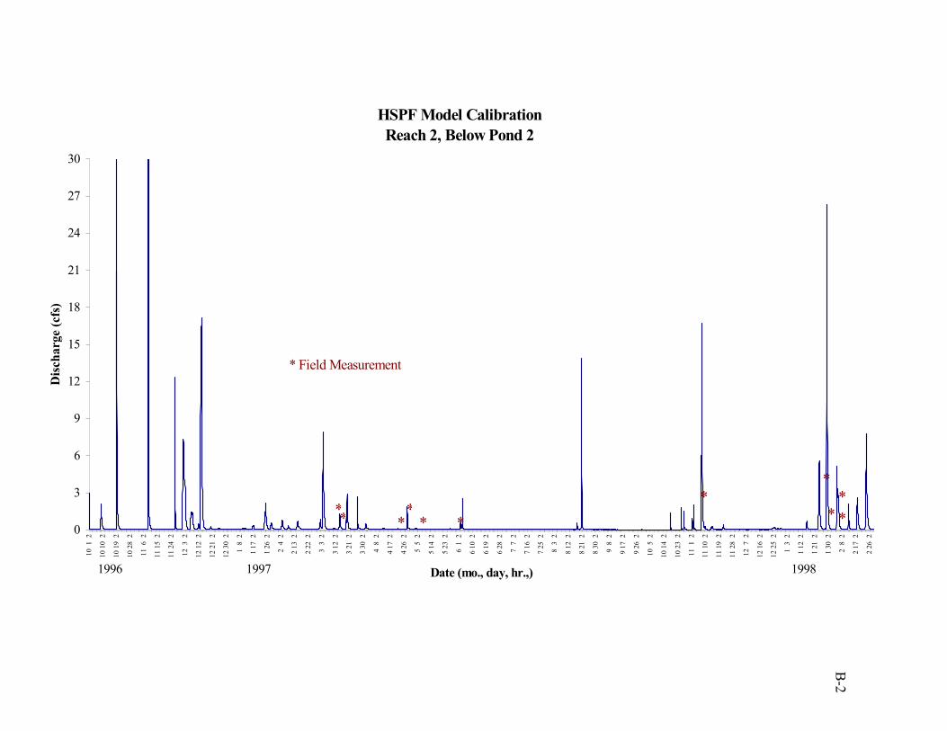
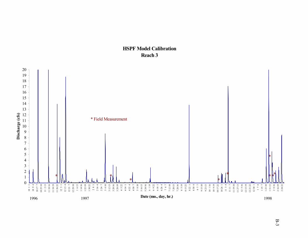
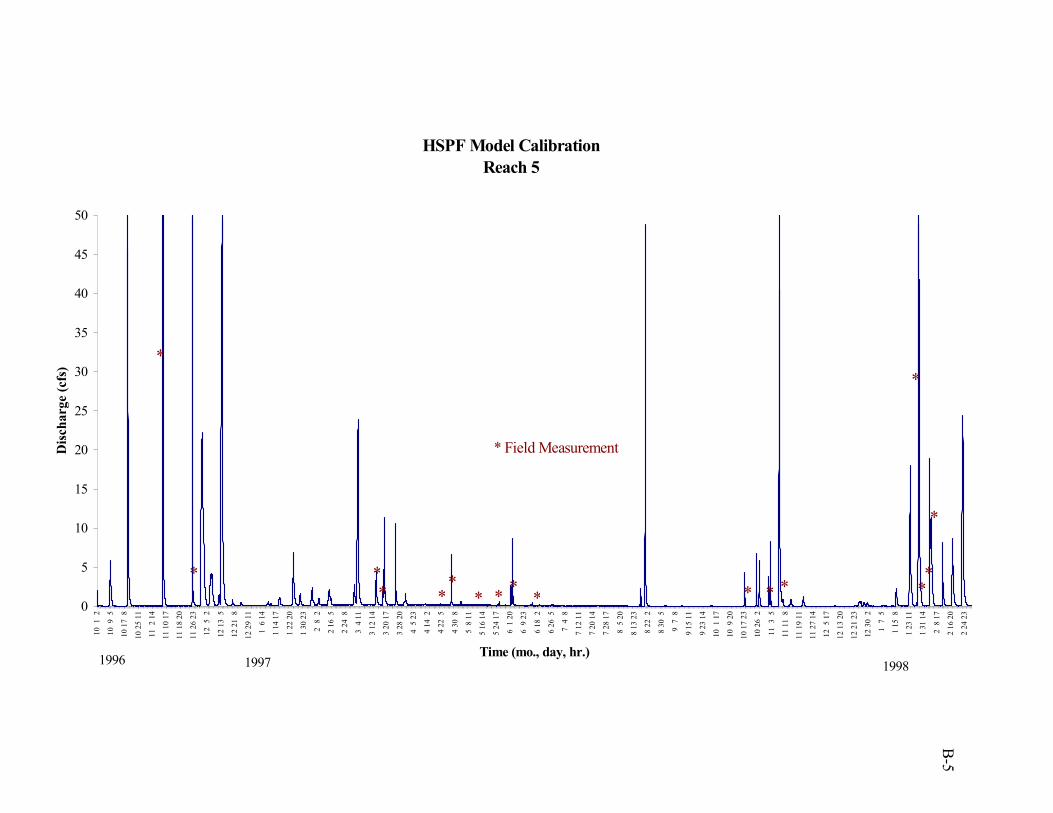
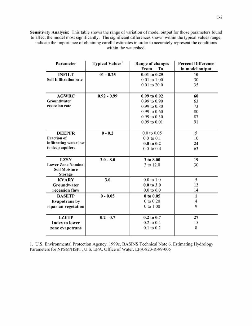
Hydrologic parameters input into the BASINS model generally describe soil processes, groundwater flow paths and evapotranspiration for each land use. The U.S. EPA BASINS Technical Note 6 (U.S. EPA, 1999c) provides guidelines for estimating these parameters based on watershed conditions. In addition, the U.S. EPA website (www.epa.gov/ost/basins/support/htm) offers the HSPFParm database (U.S. EPA, 1999d) which tabulates parameter values under a variety of watershed conditions from previous applications across North America. These sources aided in the initial determination of appropriate ranges of input parameters based on watershed conditions. Later they were also used to calibrate the model with field data. Figure 2 shows the time series of runoff flow rate for the subarea below Pond 1, called Reach 1, with the observed flow rates indicated where available. Appendix B shows the time series for the remaining segments in the Benson Branch watershed. Appendix C contains a sensitivity analysis that indicates the range of variation of model output for those parameters found to affect the model most significantly.

4

Figure 2Reach 1, Below Pond 1

0

2

4

6

8

10

12

14

16

18

20

10 1

210

9 5

10 1

7 8

10 2

5 11

11 2

14

11 1

0 17

11 1

8 20

11 2

6 23

12 5

212

13

512

21

812

29

111

6 1

41

14 1

71

22 2

01

30 2

32

8 2

2 16

52

24 8

3 4

11

3 12

14

3 20

17

3 28

20

4 5

23

4 14

24

22 5

4 30

85

8 1

15

16 1

45

24 1

76

1 2

06

9 2

36

18 2

6 26

57

4 8

7 12

11

7 20

14

7 28

17

8 5

20

8 13

23

8 22

28

30 5

9 7

89

15 1

19

23 1

410

1 1

710

9 2

010

17

2310

26

211

3 5

11 1

1 8

11 1

9 11

11 2

7 14

12 5

17

12 1

3 20

12 2

1 23

12 3

0 2

1 7

51

15 8

1 23

11

1 31

14

2 8

17

2 16

20

2 24

23

Date (mo., day, hr.,)

Dis

char

ge (c

fs)

1996 1997 1998

*** * ** * *

*

* **

* Field Measurement

5

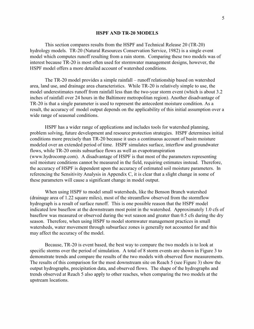
HSPF AND TR-20 MODELS

This section compares results from the HSPF and Technical Release 20 (TR-20) hydrology models. TR-20 (Natural Resources Conservation Service, 1982) is a single event model which computes runoff resulting from a rain storm. Comparing these two models was of interest because TR-20 is most often used for stormwater management designs, however, the HSPF model offers a more detailed account of watershed conditions.

The TR-20 model provides a simple rainfall – runoff relationship based on watershed

area, land use, and drainage area characteristics. While TR-20 is relatively simple to use, the model underestimates runoff from rainfall less than the two-year storm event (which is about 3.2 inches of rainfall over 24 hours in the Baltimore metropolitan region). Another disadvantage of TR-20 is that a single parameter is used to represent the antecedent moisture condition. As a result, the accuracy of model output depends on the applicability of this initial assumption over a wide range of seasonal conditions.

HSPF has a wider range of applications and includes tools for watershed planning, problem solving, future development and resource protection strategies. HSPF determines initial conditions more precisely than TR-20 because it uses a continuous account of basin moisture modeled over an extended period of time. HSPF simulates surface, interflow and groundwater flows, while TR-20 omits subsurface flows as well as evapotranspiration (www.hydrocomp.com). A disadvantage of HSPF is that most of the parameters representing soil moisture conditions cannot be measured in the field, requiring estimates instead. Therefore, the accuracy of HSPF is dependent upon the accuracy of estimated soil moisture parameters. In referencing the Sensitivity Analysis in Appendix C, it is clear that a slight change in some of these parameters will cause a significant change in model output.

When using HSPF to model small watersheds, like the Benson Branch watershed (drainage area of 1.22 square miles), most of the streamflow observed from the stormflow hydrograph is a result of surface runoff. This is one possible reason that the HSPF model indicated low baseflow at the downstream most point in the watershed. Approximately 1.0 cfs of baseflow was measured or observed during the wet season and greater than 0.5 cfs during the dry season. Therefore, when using HSPF to model stormwater management practices in small watersheds, water movement through subsurface zones is generally not accounted for and this may affect the accuracy of the model.

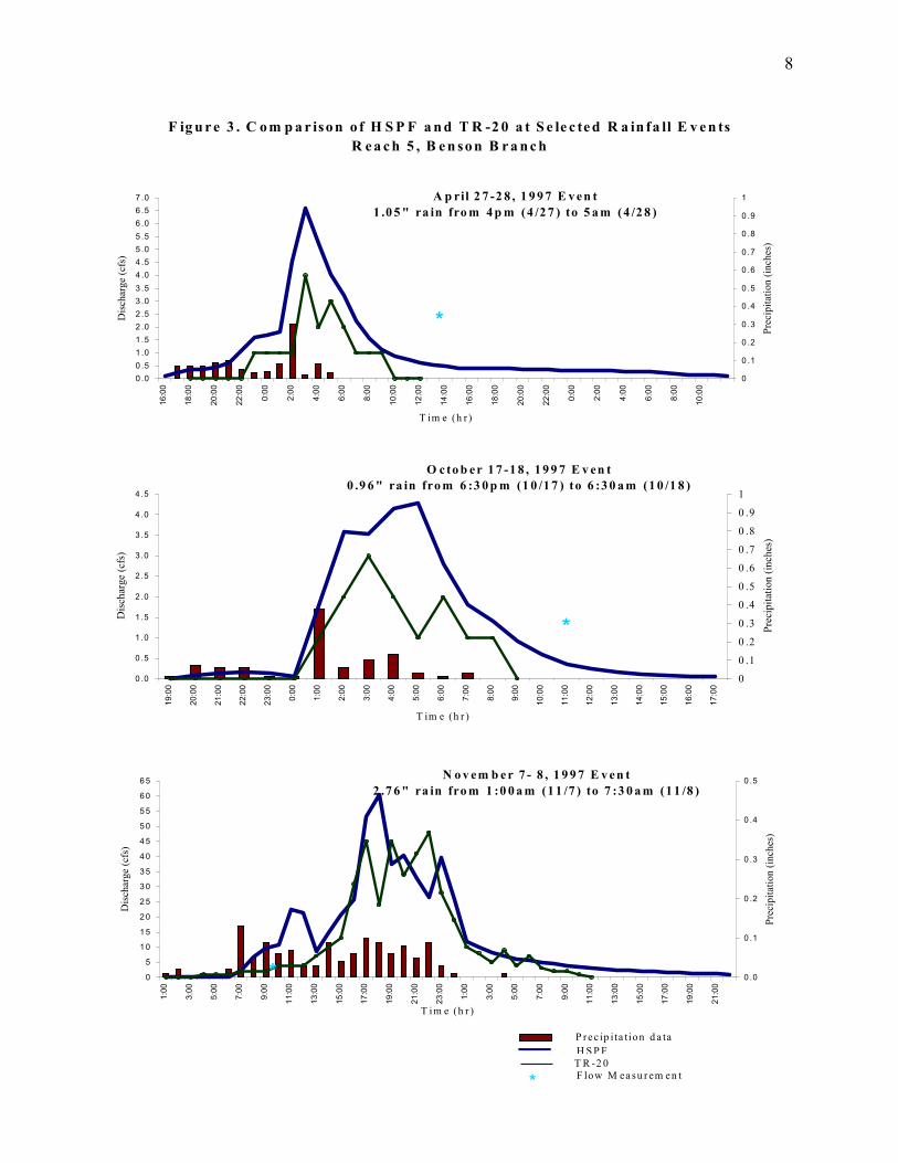
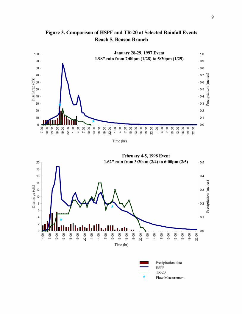
Because, TR-20 is event based, the best way to compare the two models is to look at specific storms over the period of simulation. A total of 8 storm events are shown in Figure 3 to demonstrate trends and compare the results of the two models with observed flow measurements. The results of this comparison for the most downstream site on Reach 5 (see Figure 3) show the output hydrographs, precipitation data, and observed flows. The shape of the hydrographs and trends observed at Reach 5 also apply to other reaches, when comparing the two models at the upstream locations.

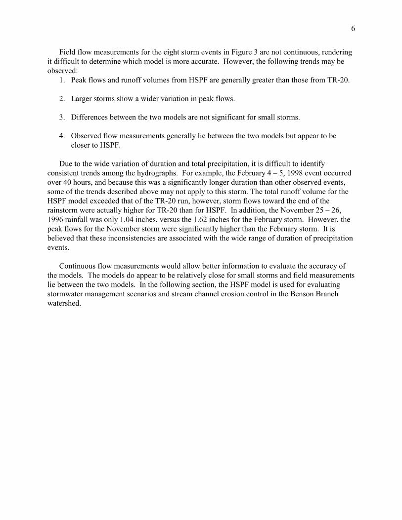
6

Field flow measurements for the eight storm events in Figure 3 are not continuous, rendering it difficult to determine which model is more accurate. However, the following trends may be observed:

1. Peak flows and runoff volumes from HSPF are generally greater than those from TR-20.

2. Larger storms show a wider variation in peak flows.

3. Differences between the two models are not significant for small storms.

4. Observed flow measurements generally lie between the two models but appear to be closer to HSPF.

Due to the wide variation of duration and total precipitation, it is difficult to identify

consistent trends among the hydrographs. For example, the February 4 – 5, 1998 event occurred over 40 hours, and because this was a significantly longer duration than other observed events, some of the trends described above may not apply to this storm. The total runoff volume for the HSPF model exceeded that of the TR-20 run, however, storm flows toward the end of the rainstorm were actually higher for TR-20 than for HSPF. In addition, the November 25 – 26, 1996 rainfall was only 1.04 inches, versus the 1.62 inches for the February storm. However, the peak flows for the November storm were significantly higher than the February storm. It is believed that these inconsistencies are associated with the wide range of duration of precipitation events.

Continuous flow measurements would allow better information to evaluate the accuracy of the models. The models do appear to be relatively close for small storms and field measurements lie between the two models. In the following section, the HSPF model is used for evaluating stormwater management scenarios and stream channel erosion control in the Benson Branch watershed.

7

F ig u r e 3 . C o m p a r iso n o f H S P F a n d T R -2 0 a t S e le c te d R a in fa ll E v e n tsR e a c h 5 , B e n so n B r a n c h

N o v e m b e r 8 , 1 9 9 6 E v e n t3 .0 8 " ra in fro m 1 1 a m (1 1 /8 ) t o 6 :3 0 a m (1 1 /9 )

02 04 06 08 0

1 0 01 2 01 4 01 6 01 8 02 0 02 2 0

11:0

0

13:0

0

15:0

0

17:0

0

19:0

0

21:0

0

23:0

0

1:00

3:00

5:00

7:00

9:00

11:0

0

13:0

0

15:0

0

17:0

0

19:0

0

21:0

0

T im e (h r )

Dis

char

ge (c

fs)

0 .0 0

0 .5 0

1 .0 0

1 .5 0

2 .0 0

2 .5 0

Prec

ipita

tion

(inch

es)

**

N o v e m b e r 2 5 -2 6 , 1 9 9 6 E v e n t1 .0 4 " ra in fro m 1 0 :3 0 p m (1 1 /2 5 ) to 7 :3 0 a m (1 1 /2 6 )

05

1 01 52 02 53 03 54 04 55 05 56 0

23:0

0

1:00

3:00

5:00

7:00

9:00

11:0

0

13:0

0

15:0

0

17:0

0

19:0

0

21:0

0

23:0

0

1:00

3:00

5:00

7:00

T im e (h r )

Dis

char

ge (c

fs)

0

0 .2

0 .4

0 .6

0 .8

1

1 .2

1 .4

1 .6

Prec

ipita

tion

(inch

es)

*

M a rc h 1 4 , 1 9 9 7 E v e n t0 .7 0 " ra in fro m 1 a m (3 /1 4 ) to 6 :3 0 (3 /1 4 )

0

1

2

3

4

5

1:00

3:00

5:00

7:00

9:00

11:0

0

13:0

0

15:0

0

17:0

0

19:0

0

21:0

0

23:0

0

1:00

3:00

5:00

7:00

9:00

11:0

0

13:0

0

T im e (h r )

Dis

char

ge (c

fs)

0 .0 0

0 .0 6

0 .1 2

0 .1 8

0 .2 4

0 .3 0

0 .3 6

0 .4 2

0 .4 8

0 .5 4

0 .6 0

Prec

ipita

tion

(inch

es)

*

*

P re c ip i ta t io n d a taH S P FT R -2 0

* F lo w M ea su r em e n t

8

F ig u r e 3 . C o m p a r iso n o f H S P F a n d T R -2 0 a t S e le c te d R a in fa ll E v e n tsR e a c h 5 , B e n so n B r a n c h

A p ril 2 7 -2 8 , 1 9 9 7 E v e n t1 .0 5 " ra in fro m 4 p m (4 /2 7 ) to 5 a m (4 /2 8 )

0 .00 .51 .01 .52 .02 .53 .03 .54 .04 .55 .05 .56 .06 .57 .0

16:0

0

18:0

0

20:0

0

22:0

0

0:00

2:00

4:00

6:00

8:00

10:0

0

12:0

0

14:0

0

16:0

0

18:0

0

20:0

0

22:0

0

0:00

2:00

4:00

6:00

8:00

10:0

0

T im e (h r )

Dis

char

ge (c

fs)

0

0 .1

0 .2

0 .3

0 .4

0 .5

0 .6

0 .7

0 .8

0 .9

1

Prec

ipita

tion

(inch

es)

*

O c to b e r 1 7 -1 8 , 1 9 9 7 E v en t0 .9 6 " ra in fro m 6 :3 0 p m (1 0 /1 7 ) to 6 :3 0 a m (1 0 /1 8 )

0 .0

0 .5

1 .0

1 .5

2 .0

2 .5

3 .0

3 .5

4 .0

4 .5

19:0

0

20:0

0

21:0

0

22:0

0

23:0

0

0:00

1:00

2:00

3:00

4:00

5:00

6:00

7:00

8:00

9:00

10:0

0

11:0

0

12:0

0

13:0

0

14:0

0

15:0

0

16:0

0

17:0

0T im e (h r )

Dis

char

ge (c

fs)

0

0 .1

0 .2

0 .3

0 .4

0 .5

0 .6

0 .7

0 .8

0 .9

1

Prec

ipita

tion

(inch

es)

*

N o v em b e r 7 - 8 , 1 9 9 7 E v e n t2 .7 6 " ra in fro m 1 :0 0 a m (1 1 /7 ) to 7 :3 0 a m (1 1 /8 )

0

5

1 0

1 5

2 0

2 5

3 0

3 5

4 0

4 5

5 0

5 5

6 0

6 5

1:00

3:00

5:00

7:00

9:00

11:0

0

13:0

0

15:0

0

17:0

0

19:0

0

21:0

0

23:0

0

1:00

3:00

5:00

7:00

9:00

11:0

0

13:0

0

15:0

0

17:0

0

19:0

0

21:0

0

T im e (h r )

Dis

char

ge (c

fs)

0 .0

0 .1

0 .2

0 .3

0 .4

0 .5Pr

ecip

itatio

n (in

ches

)

*

P recip i ta tion d a taH S P FT R -2 0

* F low M ea su r em en t

9

Reach 5, Benson BranchFigure 3. Comparison of HSPF and TR-20 at Selected Rainfall Events

February 4-5, 1998 Event1.62" rain from 3:30am (2/4) to 6:00pm (2/5)

0

2

4

6

8

10

12

14

16

18

20

4:00

7:00

10:0

0

13:0

0

16:0

0

19:0

0

22:0

0

1:00

4:00

7:00

10:0

0

13:0

0

16:0

0

19:0

0

22:0

0

1:00

4:00

7:00

10:0

0

13:0

0

16:0

0

19:0

0

22:0

0

Time (hr)

Dis

char

ge (c

fs)

0.0

0.1

0.2

0.3

0.4

0.5

Prec

ipita

tion

(inch

es)

**

January 28-29, 1997 Event1.98" rain from 7:00pm (1/28) to 5:30pm (1/29)

0

10

20

30

40

50

60

70

80

90

100

7:00

10:0

0

13:0

0

16:0

0

19:0

0

22:0

0

1:00

4:00

7:00

10:0

0

13:0

0

16:0

0

19:0

0

22:0

0

1:00

4:00

7:00

10:0

0

13:0

0

16:0

0

19:0

0

22:0

0

1:00

4:00

7:00

10:0

0

13:0

0

16:0

0

19:0

0

22:0

0

Time (hr)

Dis

char

ge (c

fs)

0.0

0.1

0.2

0.3

0.4

0.5

0.6

0.7

0.8

0.9

1.0

Prec

ipita

iton

(inch

es)

*

*

Precipitation dataHSPFTR-20

* Flow Measurement

10

STORMWATER MANAGEMENT SCENARIOS Scenario Development

The main objective in developing an HSPF model for the Benson Branch watershed is to evaluate the effectiveness of various management strategies for protecting stream channels. Using HSPF, four stormwater management designs are simulated for Pond 1 and Pond 2. The designs include existing ponds, 2 year peak management, channel protection volume (Cpv), and the Distributed Runoff Control method (DRC). The designs are evaluated to model the effects of the duration of runoff on the receiving stream channel and to determine the most effective protection practice.

The first pond scenario represents existing watershed conditions. Ponds 1 and 2 were constructed for flood control and irrigation and do not meet current stormwater management regulatory requirements. Computations do show, however, that both ponds provide management for the 10 year storm. Stage-storage-discharge relationships (see the F-TABLES in Appendix A) represent the existing ponds.

The 2 year management design is based on attenuating discharges so that the pre-development peak flow for the 2 year, 24 hour storm event is not exceeded under post development conditions. The storage capacity required to maintain peak flows below a specified discharge is determined using the procedure outlined in Chapter 6 of the Technical Release 55 (TR-55) manual published by the NRCS. This establishes a new storage volume-discharge relationship. F-TABLES for the HSPF model are modified for the reaches below Ponds 1 and 2 (Reaches 1 and 2 respectively) to represent this new relationship, and are shown in Appendix A.

The Cpv scenario is based on a 24 hour delay between the centroids of the inflow and outflow hydrographs for the 1 year frequency storm. The design procedure follows the methodology outlined in MDE’s Design Procedures For Stormwater Management Extended Detention Structures (MDE, 1987a). A new stage-storage-discharge relationship was established for Reaches 1 and 2 for the channel protection design and shown in the F-TABLES in Appendix A.

The State of Maryland is proposing the Cpv design for stream channel protection in the 2000 Maryland Stormwater Design Manual Volume I and II (MDE, 2000). This is significant because only one percent of all annual events will exceed the 1 year frequency storm (MDE, 2000). The philosophy is to provide attenuation for the more frequent storm events so that these discharges will be released at a rate that critical erosive velocities will seldom be exceeded. Using this procedure, peak outflow discharge is based on drainage area characteristics, and time of concentration in the watershed. The channel protection criteria using this method however, does not account for channel morphology or the composition of bed materials in the receiving stream.

The last procedure used for this analysis is called the Distributed Runoff Control (DRC) method, so named because of the non-uniform distribution of storage by stage (MacRae, 1993). The intent of the DRC approach is to minimize the potential for instream erosion for a range of

11

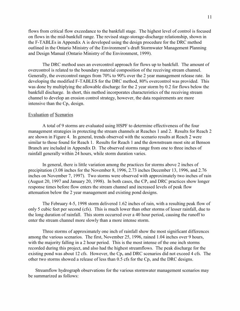
flows from critical flow exceedance to the bankfull stage. The highest level of control is focused on flows in the mid-bankfull range. The revised stage-storage-discharge relationship, shown in the F-TABLEs in Appendix A is developed using the design procedure for the DRC method outlined in the Ontario Ministry of the Environment’s draft Stormwater Management Planning and Design Manual (Ontario Ministry of the Environment, 1999).

The DRC method uses an overcontrol approach for flows up to bankfull. The amount of overcontrol is related to the boundary material composition of the receiving stream channel. Generally, the overcontrol ranges from 70% to 90% over the 2 year management release rate. In developing the modified F-TABLES for the DRC method, 80% overcontrol was provided. This was done by multiplying the allowable discharge for the 2 year storm by 0.2 for flows below the bankfull discharge. In short, this method incorporates characteristics of the receiving stream channel to develop an erosion control strategy, however, the data requirements are more intensive than the Cpv design. Evaluation of Scenarios

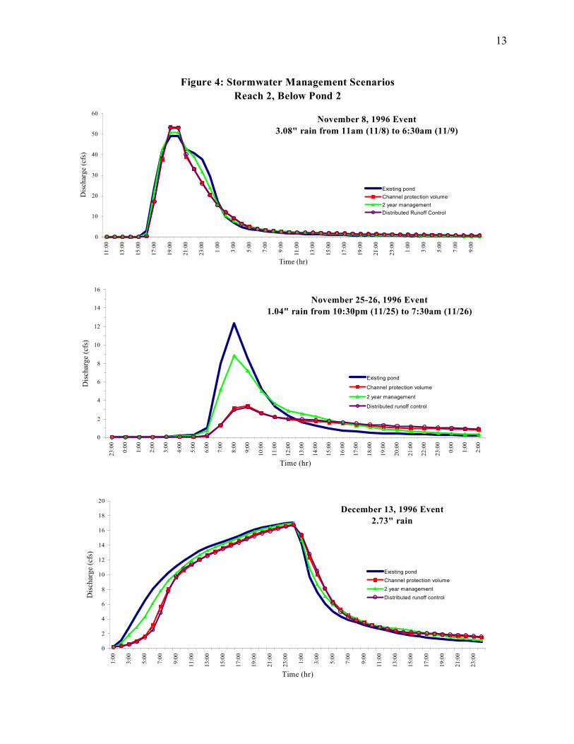
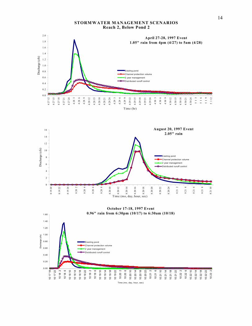
A total of 9 storms are evaluated using HSPF to determine effectiveness of the four management strategies in protecting the stream channels at Reaches 1 and 2. Results for Reach 2 are shown in Figure 4. In general, trends observed with the scenario results at Reach 2 were similar to those found for Reach 1. Results for Reach 1 and the downstream most site at Benson Branch are included in Appendix D. The observed storms range from one to three inches of rainfall generally within 24 hours, while storm duration varies.

In general, there is little variation among the practices for storms above 2 inches of precipitation (3.08 inches for the November 8, 1996, 2.73 inches December 13, 1996, and 2.76 inches on November 7, 1997). Two storms were observed with approximately two inches of rain (August 20, 1997 and January 20, 1998). In both cases, the CPv and DRC practices show longer response times before flow enters the stream channel and increased levels of peak flow attenuation below the 2 year management and existing pond designs.

The February 4-5, 1998 storm delivered 1.62 inches of rain, with a resulting peak flow of only 5 cubic feet per second (cfs). This is much lower than other storms of lesser rainfall, due to the long duration of rainfall. This storm occurred over a 40 hour period, causing the runoff to enter the stream channel more slowly than a more intense storm.

Three storms of approximately one inch of rainfall show the most significant differences among the various scenarios. The first, November 25, 1996, rained 1.04 inches over 9 hours, with the majority falling in a 2 hour period. This is the most intense of the one inch storms recorded during this project, and also had the highest streamflows. The peak discharge for the existing pond was about 12 cfs. However, the Cpv and DRC scenarios did not exceed 4 cfs. The other two storms showed a release of less than 0.5 cfs for the Cpv and the DRC designs.

Streamflow hydrograph observations for the various stormwater management scenarios may be summarized as follows:

12

1. Hydrographs for the Cpv and DRC designs are not significantly different for the storms observed. Accordingly, the Cpv and DRC designs offer the same degree of channel protection for the two ponds observed in this study.

2. The Cpv and DRC methods provide the greatest protection for storms with less than 2 inches of rainfall. For storms greater than 2 inches, the Cpv and DRC hydrographs resemble the hydrographs for the existing pond and 2 year management scenarios.

This analysis focuses on comparing stormflow hydrographs under various scenarios. The

next section provides an analysis of channel stability thresholds, to determine the effectiveness of various designs in protecting stream channels. Channel stability thresholds are based on channel morphology and stream bed composition.

13

Figure 4: Stormwater Management ScenariosReach 2, Below Pond 2

November 8, 1996 Event3.08" rain from 11am (11/8) to 6:30am (11/9)

0

10

20

30

40

50

6011

:00

13:0

0

15:0

0

17:0

0

19:0

0

21:0

0

23:0

0

1:00

3:00

5:00

7:00

9:00

11:0

0

13:0

0

15:0

0

17:0

0

19:0

0

21:0

0

23:0

0

1:00

3:00

5:00

7:00

9:00

Time (hr)

Dis

char

ge (c

fs)

Existing pond Channel protection volume2 year managementDistributed Runoff Control

November 25-26, 1996 Event1.04" rain from 10:30pm (11/25) to 7:30am (11/26)

0

2

4

6

8

10

12

14

16

23:0

0

0:00

1:00

2:00

3:00

4:00

5:00

6:00

7:00

8:00

9:00

10:0

0

11:0

0

12:0

0

13:0

0

14:0

0

15:0

0

16:0

0

17:0

0

18:0

0

19:0

0

20:0

0

21:0

0

22:0

0

23:0

0

0:00

1:00

2:00

Time (hr)

Dis

char

ge (c

fs)

Existing pond

Channel protection volume

2 year management

Distributed runoff control

December 13, 1996 Event2.73" rain

0

2

4

6

8

10

12

14

16

18

20

1:00

3:00

5:00

7:00

9:00

11:0

0

13:0

0

15:0

0

17:0

0

19:0

0

21:0

0

23:0

0

1:00

3:00

5:00

7:00

9:00

11:0

0

13:0

0

15:0

0

17:0

0

19:0

0

21:0

0

23:0

0

Time (hr)

Dis

char

ge (c

fs)

Existing pondChannel protection volume2 year managementDistributed runoff control

14

STORM WATER MANAGEMENT SCENARIOSReach 2, Below Pond 2

April 27-28, 1997 Event1.05" rain from 4pm (4/27) to 5am (4/28)

0.0

0.2

0.4

0.6

0.8

1.0

1.2

1.4

1.6

1.8

2.0

4 27

12

4 27

15

4 27

18

4 27

21

4 27

24

4 28

3

4 28

6

4 28

9

4 28

12

4 28

15

4 28

18

4 28

21

4 28

24

4 29

3

4 29

6

4 29

9

4 29

12

4 29

15

4 29

18

4 29

21

4 29

24

4 30

3

4 30

6

4 30

9

4 30

12

4 30

15

4 30

18

4 30

21

4 30

24

5 1

3

5 1

6

5 1

9

5 1

12

T ime (hr)

Dis

char

ge (c

fs)


October 17-18, 1997 Event0.96" rain from 6:30pm (10/17) to 6:30am (10/18)

0.00

0.20

0.40

0.60

0.80

1.00

1.20

1.40

1.60

10 1

7 18

10 1

7 22

10 1

8 2

10 1

8 6

10 1

8 10

10 1

8 14

10 1

8 18

10 1

8 22

10 1

9 2

10 1

9 6

10 1

9 10

10 1

9 14

10 1

9 18

10 1

9 22

10 2

0 2

10 2

0 6

10 2

0 10

10 2

0 14

10 2

0 18

10 2

0 22

10 2

1 2

10 2

1 6

10 2

1 10

10 2

1 14

10 2

1 18

10 2

1 22

10 2

2 2

10 2

2 6

10 2

2 10

10 2

2 14

10 2

2 18

10 2

2 22

10 2

3 2

Time (mo, day, hour, sec)

Dis

char

ge (c

fs)

Exisiting pondChannel protection volume

2 year management

Distributed runoff control

August 20, 1997 Event2.05" rain

0

2

4

6

8

10

12

14

16

8 19

20

8 19

22

8 19

24

8 20

2

8 20

4

8 20

6

8 20

8

8 20

10

8 20

12

8 20

14

8 20

16

8 20

18

8 20

20

8 20

22

8 20

24

8 21

2

8 21

4

8 21

6

8 21

8

8 21

10

T ime (mo, day, hour, sec)

Dis

char

ge (c

fs)


15

STO RM W ATER M ANAGEM ENT SCENARIO Scont'd

REACH 2, Below Pond 2 Novem ber 7-8, 1997 Event

2.76" rain from 1:00am (11/7) to 7:30am (11/8)

0

2

4

6

8

10

12

14

16

18

2011

7 1

11 7

5

11 7

9

11 7

13

11 7

17

11 7

21

11 8

1

11 8

5

11 8

9

11 8

13

11 8

17

11 8

21

11 9

1

11 9

5

11 9

9

11 9

13

11 9

17

11 9

21

11 1

0 1

11 1

0 5

11 1

0 9

11 1

0 13

11 1

0 17

11 1

0 21

11 1

1 1

11 1

1 5

11 1

1 9

T ime (m o, day, hour, sec)

Dis

char

ge (c

fs)

Exis ting pond

C hannel protect ion volume

2 year management

D is tributed runoff control

R EAC H 2, B elow Pond 2 February 4-5, 1998 Ev ent

1.62" rain from 3:30am (2/4) to 6:00pm (2/5)

0

1

2

3

4

5

6

2 4

1

2 4

7

2 4

13

2 4

19

2 5

1

2 5

7

2 5

13

2 5

19

2 6

1

2 6

7

2 6

13

2 6

19

2 7

1

2 7

7

2 7

13

2 7

19

2 8

1

2 8

7

2 8

13

2 8

19

2 9

1

2 9

7

2 9

13

2 9

19

2 10

1

2 10

7

2 10

13

2 10

19

2 11

1

2 11

7

2 11

13

T im e (m o, day, hour, sec)

Dis

char

ge (c

fs)

Exis ting pond

C hannel protection volum e

2 year m anagem ent

D istributed runoff control

R EAC H 2, B elow Pond 2 January 27-28, 1998 Ev ent

1.98" rain from 7pm (1/28) to 5:30pm (1/29)

0

5

10

15

20

25

30

1 27

12

1 27

14

1 27

16

1 27

18

1 27

20

1 27

22

1 27

24

1 28

2

1 28

4

1 28

6

1 28

8

1 28

10

1 28

12

1 28

14

1 28

16

1 28

18

1 28

20

1 28

22

1 28

24

1 29

2

1 29

4

1 29

6

1 29

8

1 29

10

1 29

12

1 29

14

1 29

16

1 29

18

1 29

20

1 29

22

1 29

24

1 30

2

T ime (m o, day, hour, sec)

Dis

char

ge (c

fs)

Exis ting pond

C hannel protection volume

2 year management

D is tributed runoff control

16

CHANNEL STABILITY ANALYSIS

The analysis of stormwater management scenarios shows that the Cpv and DRC designs provide significantly more attenuation of runoff than the 2-year design for smaller storms. The analysis also shows that Cpv and DRC provide a comparable level of management for ponds simulated in this watershed. The analysis, however, does not show the level of management necessary to protect the stream channel. This section provides an analysis of channel stability thresholds to further evaluate the effectiveness of stormwater management strategies for channel protection.

A bankfull elevation was determined for each stream reach during the assessment phase (MDE, 1999). Streams with poorly defined floodplains and incised channels, however, often make definition of the bankfull elevation a difficult field determination. The equations used in this analysis are then based on channel hydraulic geometry and do not require bankfull data.

A stage – discharge – shear stress relationship is established using WINXSPRO channel

cross-section analyzer (U.S. Forest Service, 1997). Data required includes channel geometry and a Manning’s n value assigned at various stages within the channel cross-section. These cross-section data were measured in the field and the n values were calculated at low stages, using observed flow and channel geometry measurements, and by applying the Manning’s equation:

))()()((

486.12

13

2

SRAQn =

where Q equals discharge, A is cross-sectional area, R is the hydraulic radius and S is the channel slope. Estimates of n values at high flows are based on the characteristics of the channel and floodplain. Table 2 provides an example of the stage – discharge – shear stress relationship established using WINXSPRO channel cross-section analyzer.

The shear stress ratio is used as an indicator of stability at various stages (or depth) within the channel. The shear stress ratio is the ratio of the average boundary shear stress to the critical shear stress and can be defined by the equation (Johnson, et. al, 1999):

c

oe τ

ττ =

where τe = the shear stress ratio, τo = the average boundary shear stress, and τc = the critical shear stress at which grain movement is initiated. The average boundary shear stress is defined by:

RSo γτ =

where γ = the specific weight of water, R = the hydraulic radius, and S = channel slope. In reference to Table 2, the average boundary shear (τo) is calculated at different depths in the channel. The WINXSPRO program can calculate hydraulic radius by using the channel cross-section data, and the cross-sectional area and wetted perimeter are computed at different depths. The critical shear stress (τc) is then calculated using the Shields equation for critical shear stress (Johnson et. al, 1999):

Dsc )( γγθτ −=

17

where τc is critical shear stress, θ = Shields parameter, γs = specific weight of sediment, γ = specific weight of water, and D is particle size. The Shield’s parameter is a function of particle size and the density of particle arrangement. Particle size at each cross-section was collected in the field according to the procedure in Wolman, 1954 and reported in MDE, 1999. The median size of bed materials, D50, is used as the representative diameter (Gordon et. al, 1992).

The shear stress ratio is calculated by dividing the average boundary shear stress at a given stage by the critical shear stress. This provides a shear stress ratio at various depths within the channel cross-section. When the shear stress ratio is less than 1.0, grain motion will not occur and the channel is considered stable. From Table 2, the depth at which the shear stress ratio is greater than 1.0 can be determined.

A channel is considered stable in form when the shear stress is approximately 20%

greater than that required to initiate motion in the center of the channel (Prestegaard et. al, 2000). This would provide a shear stress ratio (τo / τc) of less than 1.2. Parker, 1979 supports this

STAGE Q SHEAR SS Ratio (ft) (cfs) (psf)0.0 0.00 0.01 0.020.1 0.05 0.06 0.150.2 0.47 0.14 0.340.3 1.61 0.25 0.610.4 3.61 0.39 0.950.5 6.20 0.53 1.290.6 9.39 0.66 1.610.7 13.10 0.78 1.900.8 17.33 0.90 2.200.9 22.05 0.82 2.001.0 27.43 0.82 2.001.1 33.56 0.89 2.171.2 40.43 0.96 2.341.3 48.10 1.06 2.591.4 56.33 1.14 2.781.5 63.97 1.23 3.001.6 71.84 1.31 3.201.7 81.31 1.38 3.371.8 91.60 1.45 3.541.9 103.01 1.57 3.832.0 115.03 1.68 4.10

Table 2. Stage - Discharge - Shear Stress - Shear Stress Ratio RelationshipReach 2

18

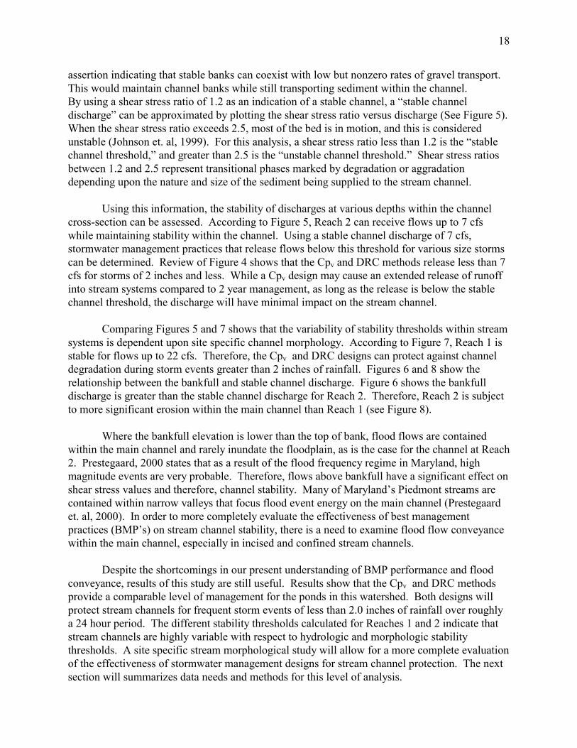
assertion indicating that stable banks can coexist with low but nonzero rates of gravel transport. This would maintain channel banks while still transporting sediment within the channel. By using a shear stress ratio of 1.2 as an indication of a stable channel, a “stable channel discharge” can be approximated by plotting the shear stress ratio versus discharge (See Figure 5). When the shear stress ratio exceeds 2.5, most of the bed is in motion, and this is considered unstable (Johnson et. al, 1999). For this analysis, a shear stress ratio less than 1.2 is the “stable channel threshold,” and greater than 2.5 is the “unstable channel threshold.” Shear stress ratios between 1.2 and 2.5 represent transitional phases marked by degradation or aggradation depending upon the nature and size of the sediment being supplied to the stream channel.

Using this information, the stability of discharges at various depths within the channel cross-section can be assessed. According to Figure 5, Reach 2 can receive flows up to 7 cfs while maintaining stability within the channel. Using a stable channel discharge of 7 cfs, stormwater management practices that release flows below this threshold for various size storms can be determined. Review of Figure 4 shows that the Cpv and DRC methods release less than 7 cfs for storms of 2 inches and less. While a Cpv design may cause an extended release of runoff into stream systems compared to 2 year management, as long as the release is below the stable channel threshold, the discharge will have minimal impact on the stream channel.

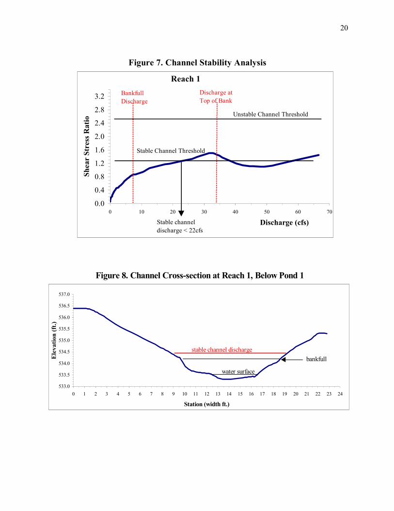
Comparing Figures 5 and 7 shows that the variability of stability thresholds within stream systems is dependent upon site specific channel morphology. According to Figure 7, Reach 1 is stable for flows up to 22 cfs. Therefore, the Cpv and DRC designs can protect against channel degradation during storm events greater than 2 inches of rainfall. Figures 6 and 8 show the relationship between the bankfull and stable channel discharge. Figure 6 shows the bankfull discharge is greater than the stable channel discharge for Reach 2. Therefore, Reach 2 is subject to more significant erosion within the main channel than Reach 1 (see Figure 8).

Where the bankfull elevation is lower than the top of bank, flood flows are contained within the main channel and rarely inundate the floodplain, as is the case for the channel at Reach 2. Prestegaard, 2000 states that as a result of the flood frequency regime in Maryland, high magnitude events are very probable. Therefore, flows above bankfull have a significant effect on shear stress values and therefore, channel stability. Many of Maryland’s Piedmont streams are contained within narrow valleys that focus flood event energy on the main channel (Prestegaard et. al, 2000). In order to more completely evaluate the effectiveness of best management practices (BMP’s) on stream channel stability, there is a need to examine flood flow conveyance within the main channel, especially in incised and confined stream channels.

Despite the shortcomings in our present understanding of BMP performance and flood conveyance, results of this study are still useful. Results show that the Cpv and DRC methods provide a comparable level of management for the ponds in this watershed. Both designs will protect stream channels for frequent storm events of less than 2.0 inches of rainfall over roughly a 24 hour period. The different stability thresholds calculated for Reaches 1 and 2 indicate that stream channels are highly variable with respect to hydrologic and morphologic stability thresholds. A site specific stream morphological study will allow for a more complete evaluation of the effectiveness of stormwater management designs for stream channel protection. The next section will summarizes data needs and methods for this level of analysis.

19

Figure 5. Channel Stability Analysis

Reach 2

0.00.40.81.21.62.02.42.83.23.64.04.44.85.25.66.0

0 10 20 30 40 50 60 70 80 90 100 110 120 130 140 150 160 170 180

Discharge (cfs)

Shea

r St

ress

Rat

ioBankfull Discharge

Discharge atTop of Bank

Stable Channel Threshold

Unstable Channel Threshold

Stable channel discharge <7cfs

Figure 6. Channel Cross-section at Reach 2, Below Pond 2

517.5

518.0

518.5

519.0

519.5

520.0

520.5

521.0

521.5

0 2 4 6 8 10 12 14 16 18 20 22 24 26 28 30 32 34 36 38 40 42Station (width ft.)

Ele

vatio

n (f

t.)

water surface

bankfullstable channeldischarge

20

Figure 7. Channel Stability Analysis

Reach 1

0.0

0.4

0.8

1.2

1.6

2.0

2.4

2.8

3.2

0 10 20 30 40 50 60 70

Discharge (cfs)

Shea

r St

ress

Rat





Stable channel discharge < 22cfs

Figure 8. Channel Cross-section at Reach 1, Below Pond 1

533.0

533.5

534.0

534.5

535.0

535.5

536.0

536.5

537.0

0 1 2 3 4 5 6 7 8 9 10 11 12 13 14 15 16 17 18 19 20 21 22 23 24

Station (width ft.)

Ele

vatio

n (f

t.)

water surface

bankfullstable channel discharge

21

GUIDELINES FOR EVALUATING STORMWATER MANAGEMENT DESIGNS FOR STREAM CHANNEL PROTECTION

This section discusses methods and data needs for evaluating the effectiveness of existing

stormwater management facilities for stream channel protection. The following protocol is intended as a starting point for analysis, however, as more data becomes available, field techniques and methodologies may be revised. The major steps that follow include:

1. Assess stream geomorphic conditions and identify stability thresholds. 2. Determine the relationship between stability thresholds, bankfull, top of bank, floodplain

and design storm discharges. 3. Compare stability thresholds with the release rate for the design storm of the facility.

Stream Channel Geomorphic Assessment • Conduct a stream stability analysis (Pfankuch, 1975 or Johnson et. al, 1999) to determine

various factors influencing channel stability. • Measure channel cross-sections, water surface gradients and particle size distribution

(Rosgen, 1996, Harrelson, et. al, 1994 and Wolman, 1954). • Survey several cross-sections along a stream reach to obtain reach – averaged values of

stream width, depth, area, grain size, gradient and shear stress (Harrelson, et. al, 1994). The bankfull and floodplain elevations are identified with respect to channel geometry.

• Establish channel geometry relationships using WINXSPRO or other channel cross-section analyzer. These relationships must be consistent with observed flow measurements and field verified channel hydraulic characteristics.

• Calculate critical shear stress (Shields equation), and a shear stress ratio at variable depths along the channel cross-section. Establish a discharge - shear stress ratio relationship.

• Determine stability thresholds by determining the flows which exceed a shear stress ratio of 1.2. Determine a “stable channel discharge” and associated channel stage.

• Compare the “stable channel discharge” with results from other equations which describe critical thresholds (Bathurst, 1987 and Olsen et. al, 1997): qc = 0.15g0.5 (D50)1.5 S-1.12

Stormwater Management Modeling • Calibrate stormwater management models in small watersheds with continuous in-stream

flow measurements. USGS gaging stations may be available for larger watersheds. • Assumptions in the model after calibration should be representative of field conditions. Data

requirements using HSPF are more intensive and require real time precipitation data (hourly) for the period of model development. TR-20 data requirements are more reasonable for small watersheds, however, hourly precipitation data is useful for model calibration.

• Determine the design storm that produces peak flows that exceed the stable channel discharge.

• Compare design release rates of the stormwater management facility to stable channel discharge and other channel features.

22

CONCLUSION

The overall goal for this project is to propose technical criteria for evaluating stormwater management designs and determine their effectiveness at protecting stream systems. Guidelines for evaluating stormwater management designs for stream channel protection are presented in an effort to promote further research in this area. These guidelines may be applied to other watersheds in Maryland, so that a more complete understanding of the affects of stormwater management practices on receiving stream channels may be achieved. Results from this study show that stability thresholds may be highly variable due to a range of morphologic and hydrologic conditions. Further data is also needed to evaluate the application of reach - averaged morphological data for determining channel stability thresholds. In addition research examining the affect of flood conveyance within incised stream channels is needed. This is particularly a concern in Maryland’s Piedmont, where stream channels are often confined within narrow valleys. This will help identify further needs and expand on existing knowledge in the area of stormwater management for protecting stream channels.

23

REFERENCES Bathurst J.C. 1987. Critical Conditions for Bed Material Movement in Steep, Boulder-Bed Streams. International Association of Hydrological Sciences Publication 165:309-318. Bicknell, B.R., J.C. Imhoff, J.L. Kittle, A.S. Donigian and R.C. Johanson. 1993. Hydrology Simulation Program – Fortran (HSPF): Users Manual for Release 10. EPA-600/R-93/174, U.S EPA, Athens, GA. Donigian, A.S. Jr., B.R. Bicknell, and J.C. Imhoff. 1995. Hydrology Simulation Program – Fortran (HSPF). In: Computer Modeling of Watershed Hydrology. Water Resources Publications. Highlands Ranch, CO. p. 395-442. Gordon, N.D., T.A. McMahon, and B.L. Finlayson. 1992. Stream Hydrology, An Introduction for Ecologists. John Wiley & Sons Ltd. Chichester, England. Hammer, T.R. 1972. Stream Channel Enlargement Due to Urbanization. Water Resources Research, vol 8. no. 6. 1530-1540. Harrelson, C.C., C.L. Rawlins and J.P. Potyondy. 1994. Stream Channel Reference Sites: An Illustrated Guide to Field Techniques. U.S. Forest Service. Fort Collins, CO. Harvey, M.D. and C.C. Watson. 1986. Fluvial Processes and Morphological Thresholds in Incised Channel Restoration. Water Resources Bulletin, vol 22. no. 3. 359-368. Hydrocomp, Inc. Hydrology Simulation Program – Fortran (HSPF). www.hydrocomp.com Johnson, P.A., G.L. Gleason and R.D. Hey. 1999. Rapid Assessment of Channel Stability in Vicinity of Road Crossing. Journal of Hydraulic Engineering. vol 125, no. 6, 645-651. MacRae, C.R. 1993. An Alternate Design Approach for the Control of Instream Erosion Potential in Urbanizing Watersheds. In: Proceedings of the Sixth International Conference on Urban Storm Drainage. Ontario Ministry of Environment and Energy. Ontario, Canada. MacRae, C.R. Experience from Morphological Research on Canadian Streams: Is Control of the Two-Hour Frequency Runoff Event the Best Basis for Stream Channel Protection. Aquafor Beech Limited, Kingston, Ontario. McCuen, R.H. 1979. Downstream Effects of Stormwater Management Basins. Journal of Hydraulics Division, ASCE 105 (H11): 1343-1356. Maryand Department of the Environment. 1987a. Design Procedures for Stormwater Management Extended Detention Structures. MDE, WMA. Baltimore, MD, 21224. Maryland Department of the Environment. 1987b. Stormwater Management Guidelines for State and Federal Projects. MDE, WMA. Baltimore, MD 21224.

24

Maryland Department of the Environment. 1999. Stream Response to Stormwater Management Best Management Practices in Maryland: Phase I Deliverable. MDE. WMA. Baltimore, MD, 21224. Maryland Department of the Environment. 2000. Maryland 2000 Stormwater Management Manual, draft. MDE, WMA, Baltimore, MD 21224. McCuen, R.H., G.E. Moglen, E.W. Kistler, and P.C. Simpson. 1987. Policy Guidelines for Controlling Stream Channel Erosion with Detention Basins. Maryland Department of the Environment. WMA, Baltimore, MD, 21224. Olsen, D.S., A.C. Whitaker, and D.F. Potts. 1997. Assessing Stream Channel Stability Thresholds Using Flow Competence Estimates at Bankfull Stage. Journal of the American Water Resources Association. Vol 33, no. 6. 1197-1207. Ontario Ministry of the Environment. 1999. Stormwater Management Planning and Design Manual, draft. Ontario Ministry of the Environment. Ontario, Canada. Natural Resources Conservation Service. 1982. Computer Program for Project Formulation – Hydrology. Technical Release 20. USDA, NRCS. Washington, D.C.. Natural Resources Conservation Service. 1986. Urban Hydrology for Small Watersheds. Technical Release 55. USDA, NRCS. Washington, D.C.. Parker, G. 1979. Hydraulic Geometry of Active Gravel Rivers. Journal of the Hydraulics Division. vol 105. no. HY 9. 1185-1201. Pfankuch, D.J. 1975. Stream Inventory and Channel Stability Evaluation. USDA, Forest Service, R1-75-002. Government Printing Office #696-260/200, Washington, D.C. Prestegaard K.L., S. Dusterhoff, C.E, Stoner, K. Houghton and K. Folk. 2000. Morphological and Hydrological Characteristics of Piedmont and Coastal Plain Streams in Maryland. MDE, WMA, Baltimore, MD 21224. Reid, I., I.C. Bathurst, P.A. Carling, D.E. Walling, and B.W. Webb. 1997. Sediment Erosion, Transport and Depostition. In: Applied Fluvial Geomorphology for River Engineering and Management. C.R. Thorne, R.D. Hey, and M.D. Newson (eds). John Wiley and Sons Ltd. Chichester, England. Rosgen, D. 1996. Applied River Morphology. Printed Media Companies, Minneapolis, Minnesota. Schumm, S.A. 1973. Geomorphic Thresholds and Complex Response of Drainage Systems. In: Fluvial Geomorphology, A Proceedings Volume of the Fourth Annual Geomorphology Symposia Series. M. Morisawa, (ed). Binghamton, New York, 13901.

25

Thorne, C.R., R.D. Hey, M.D. Newson. 1997. Applied Fluvial Geomorphology for River Engineering and Management. John Wiley & Sons Ltd, Chichester, England. U.S. Environmental Protection Agency. 1999a. BASINS Technical Note 1. Creating Hydraulic Function Tables (FTABLES) for Reservoirs in BASINS. U.S. EPA. Office of Water. EPA-823-R-99-006. Washington, D.C.. U.S. Environmental Protection Agency. 1999b. BASINS Technical Note 3. NPSM/HSPF Simulation Module Matrix. U.S. EPA. Office of Water. EPA-823-R-99-003. Washington, D.C.. U.S. Environmental Protection Agency. 1999c. BASINS Technical Note 6. Estimating Hydrology Parameters for NPSM/HSPF. U.S. EPA. Office of Water. EPA-823-R-99-005. Washington, D.C.. U.S. Environmental Protection Agency. 1999d. HSPFParm Database. U.S. EPA. Office of Water. Washington, D.C.. www.epa.gov/ost/basins/support/htm U.S. Forest Service. 1997. WINXSPRO: A Channel Cross-Section Analyzer. User’s Manual. USDA Forest Service, Rocky Mountain Experiment Station, Fort Collins, CO. Wolman, M.G. 1954. A Method of Sampling Coarse River Bed Material. Transactions, American Geophysical Union. 35(6): 952-956.

Appendix A Hydraulic Function Tables (F-TABLES)

Existing Pond A - 2 2 Year, 24 Hour Peak Management A - 3 1 Year, 24 Hour Extended Detention A - 4 Distributed Runoff Control A - 5

page

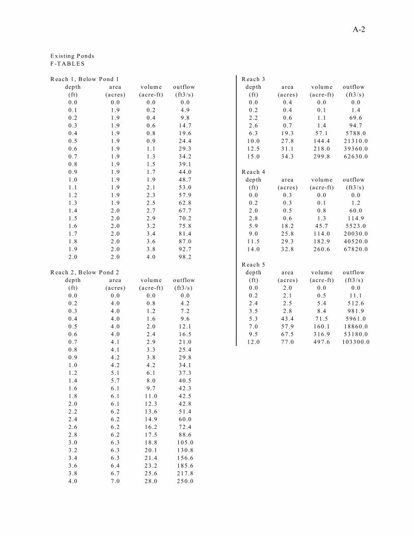
A-2

E x isting P ondsF -T A B L E S

R each 1 , B elow P ond 1 R each 3dep th a rea volum e ou tflow dep th a rea volum e ou tflow

(ft) (acres) (acre-ft) (ft3 /s) (ft) (acres) (acre-ft) (ft3 /s) 0 .0 0 .0 0 .0 0 .0 0 .0 0 .4 0 .0 0 .00 .1 1 .9 0 .2 4 .9 0 .2 0 .4 0 .1 1 .40 .2 1 .9 0 .4 9 .8 2 .2 0 .6 1 .1 69 .60 .3 1 .9 0 .6 14 .7 2 .6 0 .7 1 .4 94 .70 .4 1 .9 0 .8 19 .6 6 .3 19 .3 57 .1 5788 .00 .5 1 .9 0 .9 24 .4 10 .0 27 .8 144 .4 21310 .00 .6 1 .9 1 .1 29 .3 12 .5 31 .1 218 .0 39360 .00 .7 1 .9 1 .3 34 .2 15 .0 34 .3 299 .8 62630 .00 .8 1 .9 1 .5 39 .10 .9 1 .9 1 .7 44 .0 R each 41 .0 1 .9 1 .9 48 .7 dep th a rea volum e ou tflow 1 .1 1 .9 2 .1 53 .0 (ft) (acres) (acre-ft) (ft3 /s) 1 .2 1 .9 2 .3 57 .9 0 .0 0 .3 0 .0 0 .01 .3 1 .9 2 .5 62 .8 0 .2 0 .3 0 .1 1 .21 .4 2 .0 2 .7 67 .7 2 .0 0 .5 0 .8 60 .01 .5 2 .0 2 .9 70 .2 2 .8 0 .6 1 .3 114 .91 .6 2 .0 3 .2 75 .8 5 .9 18 .2 45 .7 5523 .01 .7 2 .0 3 .4 81 .4 9 .0 25 .8 114 .0 20030 .01 .8 2 .0 3 .6 87 .0 11 .5 29 .3 182 .9 40520 .01 .9 2 .0 3 .8 92 .7 14 .0 32 .8 260 .6 67820 .02 .0 2 .0 4 .0 98 .2

R each 5R each 2 , B elow P ond 2 dep th a rea volum e ou tflow

dep th a rea volum e ou tflow (ft) (acres) (acre-ft) (ft3 /s) (ft) (acres) (acre-ft) (ft3 /s) 0 .0 2 .0 0 .0 0 .00 .0 0 .0 0 .0 0 .0 0 .2 2 .1 0 .5 11 .10 .2 4 .0 0 .8 4 .2 2 .4 2 .5 5 .4 512 .60 .3 4 .0 1 .2 7 .2 3 .5 2 .8 8 .4 981 .90 .4 4 .0 1 .6 9 .6 5 .3 43 .4 71 .5 5961 .00 .5 4 .0 2 .0 12 .1 7 .0 57 .9 160 .1 18860 .00 .6 4 .0 2 .4 16 .5 9 .5 67 .5 316 .9 53180 .00 .7 4 .1 2 .9 21 .0 12 .0 77 .0 497 .6 103300 .00 .8 4 .1 3 .3 25 .40 .9 4 .2 3 .8 29 .81 .0 4 .2 4 .2 34 .11 .2 5 .1 6 .1 37 .31 .4 5 .7 8 .0 40 .51 .6 6 .1 9 .7 42 .31 .8 6 .1 11 .0 42 .52 .0 6 .1 12 .3 42 .82 .2 6 .2 13 .6 51 .42 .4 6 .2 14 .9 60 .02 .6 6 .2 16 .2 72 .42 .8 6 .2 17 .5 88 .63 .0 6 .3 18 .8 105 .03 .2 6 .3 20 .1 130 .83 .4 6 .3 21 .4 156 .63 .6 6 .4 23 .2 185 .63 .8 6 .7 25 .6 217 .84 .0 7 .0 28 .0 250 .0

A-3

2 year managementF T A BL E S

R ea ch 1 , B elow Pond 1 R ea ch 3depth area volume outflow depth area volume outflow

(ft) (acres) (acre-ft) (ft3 /s) (ft) (acres) (acre-ft) (ft3 /s)0 .0 0 .0 0 .0 0 .0 0 .0 0 .4 0 .0 0 .00 .1 1 .9 0 .2 1 .0 0 .2 0 .4 0 .1 1 .40 .2 1 .9 0 .4 2 .1 2 .2 0 .6 1 .1 69 .60 .3 1 .9 0 .6 4 .0 2 .6 0 .7 1 .4 94 .70 .4 1 .9 0 .8 6 .0 6 .3 19 .3 57 .1 5788.00 .5 1 .9 0 .9 9 .1 10 .0 27 .8 144.4 21310.00 .6 1 .9 1 .1 13 .1 12 .5 31 .1 218.0 39360.00 .7 1 .9 1 .3 17 .7 15 .0 34 .3 299.8 62630.00 .8 1 .9 1 .5 22 .90 .9 1 .9 1 .7 28 .5 R ea ch 41 .0 1 .9 1 .9 34 .6 depth area volume outflow1.1 1 .9 2 .1 39 .7 (ft) (acres) (acre-ft) (ft3 /s)1 .2 1 .9 2 .3 44 .8 0 .0 0 .3 0 .0 0 .01 .3 1 .9 2 .5 49 .8 0 .2 0 .3 0 .1 1 .21 .4 2 .0 2 .7 54 .9 2 .0 0 .5 0 .8 60 .01 .5 2 .0 2 .9 60 .0 2 .8 0 .6 1 .3 114.91 .6 2 .0 3 .2 66 .0 5 .9 18 .2 45 .7 5523.01 .7 2 .0 3 .4 72 .0 9 .0 25 .8 114.0 20030.01 .8 2 .0 3 .6 78 .0 11 .5 29 .3 182.9 40520.01 .9 2 .0 3 .8 84 .0 14 .0 32 .8 260.6 67820.02 .0 2 .0 4 .0 90 .0

R ea ch 5R ea ch 2 , B elow Pond 2 depth area volume outflow

depth area volume outflow (ft) (acres) (acre-ft) (ft3 /s)(ft) (acres) (acre-ft) (ft3 /s) 0 .0 2 .0 0 .0 0 .00 .0 0 .0 0 .0 0 .0 0 .2 2 .1 0 .5 11 .10 .2 4 .0 0 .8 2 .4 2 .4 2 .5 5 .4 512.60 .3 4 .0 1 .2 3 .0 3 .5 2 .8 8 .4 981.90 .4 4 .0 1 .6 4 .8 5 .3 43 .4 71 .5 5961.00 .5 4 .0 2 .0 6 .6 7 .0 57 .9 160.1 18860.00 .6 4 .0 2 .4 8 .8 9 .5 67 .5 316.9 53180.00 .7 4 .1 2 .9 11 .0 12 .0 77 .0 497.6 103300.00 .8 4 .1 3 .3 13 .80 .9 4 .2 3 .8 17 .21 .0 4 .2 4 .2 20 .91 .2 5 .1 6 .1 29 .41 .4 5 .7 8 .0 37 .91 .6 6 .1 9 .7 42 .91 .8 6 .1 11 .0 43 .12 .0 6 .1 12 .3 44 .02 .2 6 .2 13 .6 53 .22 .4 6 .2 14 .9 62 .42 .6 6 .2 16 .2 83 .22 .8 6 .2 17 .5 99 .43 .0 6 .3 18 .8 107.53 .2 6 .3 20 .1 133.33 .4 6 .3 21 .4 159.13 .6 6 .4 23 .2 204.43 .8 6 .7 25 .6 236.84 .0 7 .0 28 .0 253.0

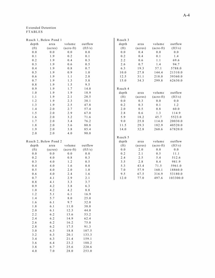
A-4

E xtended D etentionF T A B L E S

R each 1 , B elow P ond 1 R each 3depth a rea volum e outflow depth area volum e outflow

(ft) (acres) (acre-ft) (ft3 /s) (ft) (acres) (acre-ft) (ft3 /s)0 .0 0 .0 0 .0 0 .0 0 .0 0 .4 0 .0 0 .00 .1 1 .9 0 .2 0 .1 0 .2 0 .4 0 .1 1 .40 .2 1 .9 0 .4 0 .3 2 .2 0 .6 1 .1 69 .60 .3 1 .9 0 .6 0 .5 2 .6 0 .7 1 .4 94 .70 .4 1 .9 0 .8 0 .7 6 .3 19 .3 57 .1 5788 .00 .5 1 .9 0 .9 1 .0 10 .0 27 .8 144 .4 21310 .00 .6 1 .9 1 .1 2 .8 12 .5 31 .1 218 .0 39360 .00 .7 1 .9 1 .3 5 .8 15 .0 34 .3 299 .8 62630 .00 .8 1 .9 1 .5 9 .50 .9 1 .9 1 .7 14 .0 R each 41 .0 1 .9 1 .9 18 .9 depth area volum e outflow1.1 1 .9 2 .1 28 .5 (ft) (acres) (acre-ft) (ft3 /s)1 .2 1 .9 2 .3 38 .1 0 .0 0 .3 0 .0 0 .01 .3 1 .9 2 .5 47 .8 0 .2 0 .3 0 .1 1 .21 .4 2 .0 2 .7 57 .4 2 .0 0 .5 0 .8 60 .01 .5 2 .0 2 .9 67 .0 2 .8 0 .6 1 .3 114 .91 .6 2 .0 3 .2 71 .6 5 .9 18 .2 45 .7 5523 .01 .7 2 .0 3 .4 76 .2 9 .0 25 .8 114 .0 20030 .01 .8 2 .0 3 .6 80 .8 11 .5 29 .3 182 .9 40520 .01 .9 2 .0 3 .8 85 .4 14 .0 32 .8 260 .6 67820 .02 .0 2 .0 4 .0 90 .0

R each 5R each 2 , B elow P ond 2 depth area volum e outflow

depth area volum e outflow (ft) (acres) (acre-ft) (ft3 /s)(ft) (acres) (acre-ft) (ft3 /s) 0 .0 2 .0 0 .0 0 .00 .0 0 .0 0 .0 0 .0 0 .2 2 .1 0 .5 11 .10 .2 4 .0 0 .8 0 .3 2 .4 2 .5 5 .4 512 .60 .3 4 .0 1 .2 0 .5 3 .5 2 .8 8 .4 981 .90 .4 4 .0 1 .6 0 .8 5 .3 43 .4 71 .5 5961 .00 .5 4 .0 2 .0 1 .0 7 .0 57 .9 160 .1 18860 .00 .6 4 .0 2 .4 1 .6 9 .5 67 .5 316 .9 53180 .00 .7 4 .1 2 .9 2 .1 12 .0 77 .0 497 .6 103300 .00 .8 4 .1 3 .3 3 .70 .9 4 .2 3 .8 6 .31 .0 4 .2 4 .2 8 .81 .2 5 .1 6 .1 16 .91 .4 5 .7 8 .0 25 .01 .6 6 .1 9 .7 32 .01 .8 6 .1 11 .0 38 .02 .0 6 .1 12 .3 44 .02 .2 6 .2 13 .6 53 .22 .4 6 .2 14 .9 62 .42 .6 6 .2 16 .2 75 .02 .8 6 .2 17 .5 91 .33 .0 6 .3 18 .8 107 .53 .2 6 .3 20 .1 133 .33 .4 6 .3 21 .4 159 .13 .6 6 .4 23 .2 188 .23 .8 6 .7 25 .6 220 .64 .0 7 .0 28 .0 253 .0

A-5

D is tr ib u ted R u noff C on tro lF T A B L E S

R ea ch 1 , B elow P ond 1 R ea ch 3dep th a rea vo lu m e ou tflow dep th a rea vo lu m e ou tflow

(ft) (a c res ) (a c re-ft) (ft3 /s ) (ft) (a c res ) (a c re-ft) (ft3 /s )0 .0 0 .0 0 .0 0 .0 0 .0 0 .4 0 .0 0 .00 .1 1 .9 0 .2 0 .2 0 .2 0 .4 0 .1 1 .40 .2 1 .9 0 .4 0 .4 2 .2 0 .6 1 .1 6 9 .60 .3 1 .9 0 .6 0 .8 2 .6 0 .7 1 .4 9 4 .70 .4 1 .9 0 .8 1 .2 6 .3 1 9 .3 5 7 .1 5 7 8 8 .00 .5 1 .9 0 .9 1 .8 1 0 .0 2 7 .8 1 4 4 .4 2 1 3 1 0 .00 .6 1 .9 1 .1 2 .6 1 2 .5 3 1 .1 2 1 8 .0 3 9 3 6 0 .00 .7 1 .9 1 .3 3 .6 1 5 .0 3 4 .3 2 9 9 .8 6 2 6 3 0 .00 .8 1 .9 1 .5 4 .60 .9 1 .9 1 .7 1 5 .0 R ea ch 41 .0 1 .9 1 .9 2 5 .0 dep th a rea vo lu m e ou tflow1 .1 1 .9 2 .1 3 5 .0 (ft) (a c res ) (a c re-ft) (ft3 /s )1 .2 1 .9 2 .3 4 5 .0 0 .0 0 .3 0 .0 0 .01 .3 1 .9 2 .5 5 0 .0 0 .2 0 .3 0 .1 1 .21 .4 2 .0 2 .7 5 5 .0 2 .0 0 .5 0 .8 6 0 .01 .5 2 .0 2 .9 6 0 .0 2 .8 0 .6 1 .3 1 1 4 .91 .6 2 .0 3 .2 6 6 .0 5 .9 1 8 .2 4 5 .7 5 5 2 3 .01 .7 2 .0 3 .4 7 2 .0 9 .0 2 5 .8 1 1 4 .0 2 0 0 3 0 .01 .8 2 .0 3 .6 7 8 .0 1 1 .5 2 9 .3 1 8 2 .9 4 0 5 2 0 .01 .9 2 .0 3 .8 8 4 .0 1 4 .0 3 2 .8 2 6 0 .6 6 7 8 2 0 .02 .0 2 .0 4 .0 9 0 .0

R ea ch 5R ea ch 2 , B elow P ond 2 dep th a rea vo lu m e ou tflow

dep th a rea vo lu m e ou tflow (ft) (a c res ) (a c re-ft) (ft3 /s )(ft) (a c res ) (a c re-ft) (ft3 /s ) 0 .0 2 .0 0 .0 0 .00 .0 0 .0 0 .0 0 .0 0 .2 2 .1 0 .5 1 1 .10 .2 4 .0 0 .8 0 .5 2 .4 2 .5 5 .4 5 1 2 .60 .3 4 .0 1 .2 0 .6 3 .5 2 .8 8 .4 9 8 1 .90 .4 4 .0 1 .6 1 .0 5 .3 4 3 .4 7 1 .5 5 9 6 1 .00 .5 4 .0 2 .0 1 .3 7 .0 5 7 .9 1 6 0 .1 1 8 8 6 0 .00 .6 4 .0 2 .4 1 .8 9 .5 6 7 .5 3 1 6 .9 5 3 1 8 0 .00 .7 4 .1 2 .9 2 .2 1 2 .0 7 7 .0 4 9 7 .6 1 0 3 3 0 0 .00 .8 4 .1 3 .3 3 .70 .9 4 .2 3 .8 7 .01 .0 4 .2 4 .2 1 0 .01 .2 5 .1 6 .1 1 7 .01 .4 5 .7 8 .0 2 5 .51 .6 6 .1 9 .7 3 2 .01 .8 6 .1 1 1 .0 4 0 .02 .0 6 .1 1 2 .3 4 7 .02 .2 6 .2 1 3 .6 5 3 .02 .4 6 .2 1 4 .9 5 9 .02 .6 6 .2 1 6 .2 8 3 .02 .8 6 .2 1 7 .5 9 9 .03 .0 6 .3 1 8 .8 1 0 8 .03 .2 6 .3 2 0 .1 1 3 3 .03 .4 6 .3 2 1 .4 1 5 9 .03 .6 6 .4 2 3 .2 2 0 4 .03 .8 6 .7 2 5 .6 2 3 7 .04 .0 7 .0 2 8 .0 2 5 3 .0

Appendix B

HSPF Model Calibration, Reach 2, Below Pond 2 B-2 HSPF Model Calibration Reach 3 B-3 HSPF Model Calibration Reach 4 B-4 HSPF Model Calibration Reach 5 B-5

page

B-2

HSPF Model Calibration Reach 2, Below Pond 2

0

3

6

9

12

15

18

21

24

27

30

10 1

2

10 1

0 2

10 1

9 2

10 2

8 2

11 6

2

11 1

5 2

11 2

4 2

12 3

2

12 1

2 2

12 2

1 2

12 3

0 2

1 8

2

1 17

2

1 26

2

2 4

2

2 13

2

2 22

2

3 3

2

3 12

2

3 21

2

3 30

2

4 8

2

4 17

2

4 26

2

5 5

2

5 14

2

5 23

2

6 1

2

6 10

2

6 19

2

6 28

2

7 7

2

7 16

2

7 25

2

8 3

2

8 12

2

8 21

2

8 30

2

9 8

2

9 17

2

9 26

2

10 5

2

10 1

4 2

10 2

3 2

11 1

2

11 1

0 2

11 1

9 2

11 2

8 2

12 7

2

12 1

6 2

12 2

5 2

1 3

2

1 12

2

1 21

2

1 30

2

2 8

2

2 17

2

2 26

2

Date (mo., day, hr.,)

Dis

char

ge (c

fs)

1996 1997 1998

** **

* **

*

* **

* Field Measurement

B-3

HSPF Model CalibrationReach 3

0123456789

1011121314151617181920

10 1

1

10 9

4

10 1

7 7

10 2

5 10

11 2

13

11 1

0 16

11 1

8 19

11 2

6 22

12 5

1

12 1

3 4

12 2

1 7

12 2

9 10

1 6

13

1 14

16

1 22

19

1 30

22

2 8

1

2 16

4

2 24

7

3 4

10

3 12

13

3 20

16

3 28

19

4 5

22

4 14

1

4 22

4

4 30

7

5 8

10

5 16

13

5 24

16

6 1

19

6 9

22

6 18

1

6 26

4

7 4

7

7 12

10

7 20

13

7 28

16

8 5

19

8 13

22

8 22

1

8 30

4

9 7

7

9 15

10

9 23

13

10 1

16

10 9

19

10 1

7 22

10 2

6 1

11 3

4

11 1

1 7

11 1

9 10

11 2

7 13

12 5

16

12 1

3 19

12 2

1 22

12 3

0 1

1 7

4

1 15

7

1 23

10

1 31

13

2 8

16

2 16

19

2 24

22

Date (mo., day, hr.)

Dis

char

ge (c

fs)

1996 1997 1998

* Field Measurement

* ** *

*

*

***

B-4

HSPF Model Calibration Reach 4

0123456789

1011121314151617181920

10 1

1

10 9

4

10 1

7 7

10 2

5 10

11 2

13

11 1

0 16

11 1

8 19

11 2

6 22

12 5

1

12 1

3 4

12 2

1 7

12 2

9 10

1 6

13

1 14

16

1 22

19

1 30

22

2 8

1

2 16

4

2 24

7

3 4

10

3 12

13

3 20

16

3 28

19

4 5

22

4 14

1

4 22

4

4 30

7

5 8

10

5 16

13

5 24

16

6 1

19

6 9

22

6 18

1

6 26

4

7 4

7

7 12

10

7 20

13

7 28

16

8 5

19

8 13

22

8 22

1

8 30

4

9 7

7

9 15

10

9 23

13

10 1

16

10 9

19

10 1

7 22

10 2

6 1

11 3

4

11 1

1 7

11 1

9 10

11 2

7 13

12 5

16

12 1

3 19

12 2

1 22

12 3

0 1

1 7

4

1 15

7

1 23

10

1 31

13

2 8

16

2 16

19

2 24

22

Time (mo., day, hr.)

Dis

char

ge (c

fs)

1996 1997 1998

* Field Measurement

**

* **

*

**

*

B-5

HSPF Model Calibration Reach 5

0

5

10

15

20

25

30

35

40

45

50

10 1

2

10 9

5

10 1

7 8

10 2

5 11

11 2

14

11 1

0 17

11 1

8 20

11 2

6 23

12 5

2

12 1

3 5

12 2

1 8

12 2

9 11

1 6

14

1 14

17

1 22

20

1 30

23

2 8

2

2 16

5

2 24

8

3 4

11

3 12

14

3 20

17

3 28

20

4 5

23

4 14

2

4 22

5

4 30

8

5 8

11

5 16

14

5 24

17

6 1

20

6 9

23

6 18

2

6 26

5

7 4

8

7 12

11

7 20

14

7 28

17

8 5

20

8 13

23

8 22

2

8 30

5

9 7

8

9 15

11

9 23

14

10 1

17

10 9

20

10 1

7 23

10 2

6 2

11 3

5

11 1

1 8

11 1

9 11

11 2

7 14

12 5

17

12 1

3 20

12 2

1 23

12 3

0 2

1 7

5

1 15

8

1 23

11

1 31

14

2 8

17

2 16

20

2 24

23

Time (mo., day, hr.)

Dis

char

ge (c

fs)

1996 1997 1998

*

* ** *

** * * * * * *

*

*

* Field Measurement

*

*

Appendix C

Sensitivity Analysis

C-2

Sensitivity Analysis: This table shows the range of variation of model output for those parameters found to affect the model most significantly. The significant differences shown within the typical values range,

indicate the importance of obtaining careful estimates in order to accurately represent the conditions within the watershed.

Parameter Typical Values1 Range of changes From To

Percent Difference in model output

INFILT Soil Infiltration rate

01 - 0.25 0.01 to 0.25 0.01 to 1.00 0.01 to 20.0

10 30 35

AGWRC Groundwater recession rate

0.92 - 0.99 0.99 to 0.92 0.99 to 0.90 0.99 to 0.80 0.99 to 0.60 0.99 to 0.30 0.99 to 0.01

60 63 73 80 87 91

DEEPFR Fraction of infiltrating water lost to deep aquifers

0 - 0.2 0.0 to 0.05 0.0 to 0.1 0.0 to 0.2 0.0 to 0.4

5 10 24 63

LZSN Lower Zone Nominal

Soil Moisture Storage

3.0 - 8.0

3 to 8.00 3 to 12.0

19 30

KVARY Groundwater recession flow

3.0 0.0 to 1.0 0.0 to 3.0 0.0 to 6.0

5 12 14

BASETP Evapotrans by

riparian vegetation

0 - 0.05 0 to 0.05 0 to 0.20 0 to 1.00

1 4 9

LZETP Index to lower

zone evapotrans

0.2 - 0.7 0.2 to 0.7 0.2 to 0.4 0.1 to 0.2

27 15 8

1. U.S. Environmental Protection Agency. 1999c. BASINS Technical Note 6. Estimating Hydrology Parameters for NPSM/HSPF. U.S. EPA. Office of Water. EPA-823-R-99-005

Appendix D

Stormwater Management Scenarios

D-2

STORMWATER MANAGEMENT SCENARIOS

REACH 1, Below Pond 1November 8, 1996 Event

3.08" rain from 11am (11/8) to 6:30am (11/9)

0

10

20

30

40

50

60

11 8

1

11 8

3

11 8

5

11 8

7

11 8

9

11 8

11

11 8

13

11 8

15

11 8

17

11 8

19

11 8

21

11 8

23

11 9

1

11 9

3

11 9

5

11 9

7

11 9

9

11 9

11

11 9

13

11 9

15

11 9

17

11 9

19

11 9

21

11 9

23

11 1

0 1

11 1

0 3

11 1

0 5

11 1

0 7

11 1

0 9


Dis

char

ge (c

fs)

Existing pondExtended Detention2 year managementDistributed runoff control

REACH 1, Below Pond 1November 25-26, 1996 Event

1.04" rain from 10:30pm (11/25) to 7:30am (11/26)

0

1

2

3

4

5

6

7

8

9

10

11

11 2

6 1

11 2

6 2

11 2

6 3

11 2

6 4

11 2

6 5

11 2

6 6

11 2

6 7

11 2

6 8

11 2

6 9

11 2

6 10

11 2

6 11

11 2

6 12

11 2

6 13

11 2

6 14

11 2

6 15

11 2

6 16

11 2

6 17

11 2

6 18

11 2

6 19

11 2

6 20

11 2

6 21

11 2

6 22

11 2

6 23

11 2

6 24

11 2

7 1

11 2

7 2


Dis

char

ge (c

fs)


REACH 1, Below Pond 1 December 13, 1996 Event

2.73" rain

0

1

2

3

4

5

6

7

8

9

10

12 1

3 1

12 1

3 3

12 1

3 5

12 1

3 7

12 1

3 9

12 1

3 11

12 1

3 13

12 1

3 15

12 1

3 17

12 1

3 19

12 1

3 21

12 1

3 23

12 1

4 1

12 1

4 3

12 1

4 5

12 1

4 7

12 1

4 9

12 1

4 11

12 1

4 13

12 1

4 15

12 1

4 17

12 1

4 19

12 1

4 21

12 1

4 23


Dis

char

ge (c

fs)


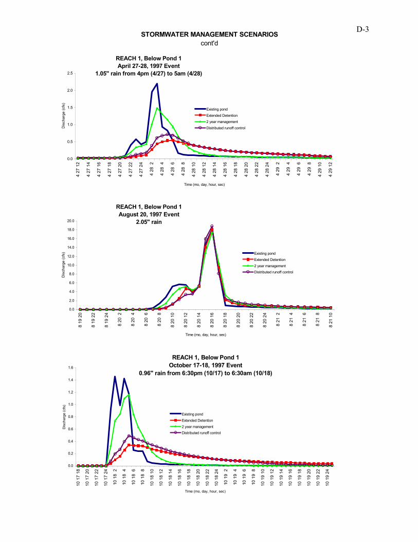
D-3

STORMWATER MANAGEMENT SCENARIOScont'd

REACH 1, Below Pond 1 April 27-28, 1997 Event

1.05" rain from 4pm (4/27) to 5am (4/28)

0.0

0.5

1.0

1.5

2.0

2.54

27 1

2

4 27

14

4 27

16

4 27

18

4 27

20

4 27

22

4 27

24

4 28

2

4 28

4

4 28

6

4 28

8

4 28

10

4 28

12

4 28

14

4 28

16

4 28

18

4 28

20

4 28

22

4 28

24

4 29

2

4 29

4

4 29

6

4 29

8

4 29

10

4 29

12


Dis

char

ge (c

fs)


REACH 1, Below Pond 1 October 17-18, 1997 Event

0.96" rain from 6:30pm (10/17) to 6:30am (10/18)

0.0

0.2

0.4

0.6

0.8

1.0

1.2

1.4

1.6

10 1

7 18

10 1

7 20

10 1

7 22

10 1

7 24

10 1

8 2

10 1

8 4

10 1

8 6

10 1

8 8

10 1

8 10

10 1

8 12

10 1

8 14

10 1

8 16

10 1

8 18

10 1

8 20

10 1

8 22

10 1

8 24

10 1

9 2

10 1

9 4

10 1

9 6

10 1

9 8

10 1

9 10

10 1

9 12

10 1

9 14

10 1

9 16

10 1

9 18

10 1

9 20

10 1

9 22

10 1

9 24


Dis

char

ge (c

fs)


REACH 1, Below Pond 1 August 20, 1997 Event

2.05" rain

0.0

2.0

4.0

6.0

8.0

10.0

12.0

14.0

16.0

18.0

20.0

8 19

20

8 19

22

8 19

24

8 20

2

8 20

4

8 20

6

8 20

8

8 20

10

8 20

12

8 20

14

8 20

16

8 20

18

8 20

20

8 20

22

8 20

24

8 21

2

8 21

4

8 21

6

8 21

8

8 21

10


Dis

char

ge (c

fs) Existing pond

Extended Detention2 year managementDistributed runoff control

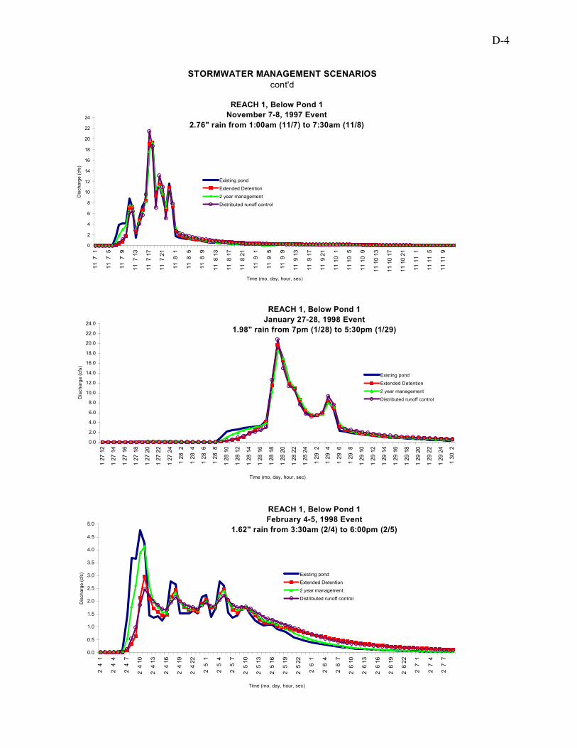
D-4

cont'dSTORMWATER MANAGEMENT SCENARIOS

REACH 1, Below Pond 1 November 7-8, 1997 Event

2.76" rain from 1:00am (11/7) to 7:30am (11/8)

0

2

4

6

8

10

12

14

16

18

20

22

24

11 7

1

11 7

5

11 7

9

11 7

13

11 7

17

11 7

21

11 8

1

11 8

5

11 8

9

11 8

13

11 8

17

11 8

21

11 9

1

11 9

5

11 9

9

11 9

13

11 9

17

11 9

21

11 1

0 1

11 1

0 5

11 1

0 9

11 1

0 13

11 1

0 17

11 1

0 21

11 1

1 1

11 1

1 5

11 1

1 9


Dis

char

ge (c

fs)


REACH 1, Below Pond 1 January 27-28, 1998 Event

1.98" rain from 7pm (1/28) to 5:30pm (1/29)

0.0

2.0

4.0

6.0

8.0

10.0

12.0

14.0

16.0

18.0

20.0

22.0

24.0

1 27

12

1 27

14

1 27

16

1 27

18

1 27

20

1 27

22

1 27

24

1 28

2

1 28

4

1 28

6

1 28

8

1 28

10

1 28

12

1 28

14

1 28

16

1 28

18

1 28

20

1 28

22

1 28

24

1 29

2

1 29

4

1 29

6

1 29

8

1 29

10

1 29

12

1 29

14

1 29

16

1 29

18

1 29

20

1 29

22

1 29

24

1 30

2


Dis

char

ge (c

fs)


REACH 1, Below Pond 1 February 4-5, 1998 Event

1.62" rain from 3:30am (2/4) to 6:00pm (2/5)

0.0

0.5

1.0

1.5

2.0

2.5

3.0

3.5

4.0

4.5

5.0

2 4

1

2 4

4

2 4

7

2 4

10

2 4

13

2 4

16

2 4

19

2 4

22

2 5

1

2 5

4

2 5

7

2 5

10

2 5

13

2 5

16

2 5

19

2 5

22

2 6

1

2 6

4

2 6

7

2 6

10

2 6

13

2 6

16

2 6

19

2 6

22

2 7

1

2 7

4

2 7

7


Dis

char

ge (c

fs) Existing pond

Extended Detention2 year managementDistributed runoff control

D-5

Storm w ater M anagem ent Scenarios

R E ACH 5Novem ber 8 , 1996 E vent

3 .08" ra in from 11am (11 /8 ) to 6 :30am (11 /9 )

0

50

100

150

200

250

11 8

1

11 8

3

11 8

5

11 8

7

11 8

9

11 8

11

11 8

13

11 8

15

11 8

17

11 8

19

11 8

21

11 8

23

11 9

1

11 9

3

11 9

5

11 9

7

11 9

9

11 9

11

11 9

13

11 9

15

11 9

17

11 9

19

11 9

21

11 9

23

11 1

0 1

11 1

0 3

11 1

0 5

11 1

0 7

11 1

0 9

T im e (m o, day, hour, sec )

Stre

amflo

w (c

fs)

Exis ting pond2 year m anagem entExtended D etentionD is tribu ted runoff contro l

R E ACH 5 Novem ber 25-26 , 1996 E vent

1 .04" ra in from 10:30pm (11 /25) to 7 :30am (11 /26)

0

10

20

30

40

50

60

11 2

5 20

11 2

5 21

11 2

5 22

11 2

5 23

11 2

5 24

11 2

6 1

11 2

6 2

11 2

6 3

11 2

6 4

11 2

6 5

11 2

6 6

11 2

6 7

11 2

6 8

11 2

6 9

11 2

6 10

11 2

6 11

11 2

6 12

11 2

6 13

11 2

6 14

11 2

6 15

11 2

6 16

11 2

6 17

11 2

6 18

11 2

6 19

11 2

6 20

11 2

6 21

11 2

6 22

11 2

6 23

11 2

6 24

11 2

7 1

11 2

7 2


Dis

char

ge (c

fs)


R E ACH 5 D ecem ber 13 , 1996 E vent

2 .73" ra in

0

10

20

30

40

50

60

12 1

3 1

12 1

3 3

12 1

3 5

12 1

3 7

12 1

3 9

12 1

3 11

12 1

3 13

12 1

3 15

12 1

3 17

12 1

3 19

12 1

3 21

12 1

3 23

12 1

4 1

12 1

4 3

12 1

4 5

12 1

4 7

12 1

4 9

12 1

4 11

12 1

4 13

12 1

4 15

12 1

4 17

12 1

4 19

12 1

4 21

12 1

4 23


Dis

char

ge (c

fs)


D-6

Stormwater Management Scenarioscont'd

REACH 5 April 27-28, 1997 Event

1.05" rain from 4pm (4/27) to 5am (4/28)

0

1

2

3

4

5

6

7

4 27

12

4 27

14

4 27

16

4 27

18

4 27

20

4 27

22

4 27

24

4 28

2

4 28

4

4 28

6

4 28

8

4 28

10

4 28

12

4 28

14

4 28

16

4 28

18

4 28

20

4 28

22

4 28

24

4 29

2

4 29

4

4 29

6

4 29

8

4 29

10

4 29

12


Dis

char

ge (c

fs)

Existing pond2 year m anagem entExtended DetentionDistributed runoff control

REACH 5 August 20, 1997 Event

2.05" rain

0

10

20

30

40

50

60

8 19

20

8 19

22

8 19

24

8 20

2

8 20

4

8 20

6

8 20

8

8 20

10

8 20

12

8 20

14

8 20

16

8 20

18

8 20

20

8 20

22

8 20

24

8 21

2

8 21

4

8 21

6

8 21

8

8 21

10


Dis

char

ge (c

fs)


REACH 5 October 17-18, 1997 Event

0.96" rain from 6:30pm (10/17) to 6:30am (10/18)

0.0

0.5

1.0

1.5

2.0

2.5

3.0

3.5

4.0

4.5

10 1

7 10

10 1

7 13

10 1

7 16

10 1

7 19

10 1

7 22

10 1

8 1

10 1

8 4

10 1

8 7

10 1

8 10

10 1

8 13

10 1

8 16

10 1

8 19

10 1

8 22

10 1

9 1

10 1

9 4

10 1

9 7

10 1

9 10

10 1

9 13

10 1

9 16

10 1

9 19

10 1

9 22

10 2

0 1


Dis

char

ge (c

fs)


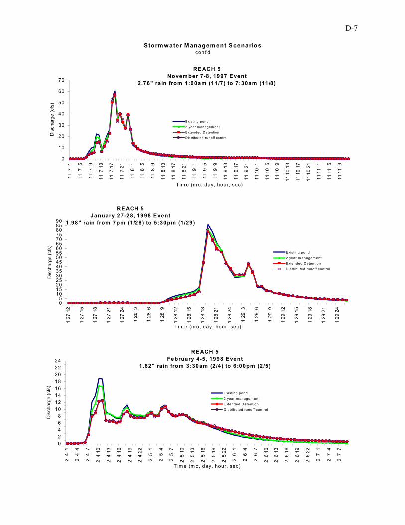
D-7

cont'dStorm w ater M anagem ent Scenarios

REACH 5 Novem ber 7-8, 1997 E vent

2.76" rain from 1:00am (11 /7) to 7:30am (11 /8)

0

10

20

30

40

50

60

70

11 7

1

11 7

5

11 7

9

11 7

13

11 7

17

11 7

21

11 8

1

11 8

5

11 8

9

11 8

13

11 8

17

11 8

21

11 9

1

11 9

5

11 9

9

11 9

13

11 9

17

11 9

21

11 1

0 1

11 1

0 5

11 1

0 9

11 1

0 13

11 1

0 17

11 1

0 21

11 1

1 1

11 1

1 5

11 1

1 9


Dis

char

ge (c

fs)

E xis ting pond2 year m anagem entExtended Deten tionD istribu ted runoff con trol

REACH 5 February 4-5, 1998 E vent

1 .62" ra in from 3:30am (2 /4 ) to 6:00pm (2 /5)

02468

1012141618202224

2 4

1

2 4

4

2 4

7

2 4

10

2 4

13

2 4

16

2 4

19

2 4

22

2 5

1

2 5

4

2 5

7

2 5

10

2 5

13

2 5

16

2 5

19

2 5

22

2 6

1

2 6

4

2 6

7

2 6

10

2 6

13

2 6

16

2 6

19

2 6

22

2 7

1

2 7

4

2 7

7


Dis

char

ge (c

fs)

Exis ting pond2 year m anagem entExtended DetentionD is tributed runoff control

RE ACH 5 January 27-28, 1998 Event

1.98" rain from 7pm (1/28) to 5 :30pm (1/29)

05

1015202530354045505560657075808590

1 27

12

1 27

15

1 27

18

1 27

21

1 27

24

1 28

3

1 28

6

1 28

9

1 28

12

1 28

15

1 28

18

1 28

21

1 28

24

1 29

3

1 29

6

1 29

9

1 29

12

1 29

15

1 29

18

1 29

21

1 29

24


Dis

char

ge (c

fs)

Exis ting pond2 year m anagem entExtended DetentionDistributed runoff control

Appendix E

Channel Stability Analysis at Benson Branch, Reach 5

E-2

Channel Stability Analysis

Benson Branch

0.00.40.81.21.62.02.42.83.23.64.04.44.85.25.66.0

0 10 20 30 40 50 60 70 80 90 100 110 120 130 140 150 160 170

Discharge (cfs)

Shea

r St

ress

Rat





Stable channeldischarge approx 8cfs

Channel Cross-section at Reach 5, on Benson Branch

452.5453.0453.5454.0454.5455.0455.5456.0456.5457.0457.5458.0458.5

0 2 4 6 8 10 12 14 16 18 20 22 24 26 28 30 32 34 36 38 40 42 44 46

Station (width ft.)

Ele

vatio

n (f

t.) bankfull

water surfacestable channel discharge

stream response to stormwater management best management

Documents