strategies for non linear system identification · type of non-linearity. ... simulated data for a...
TRANSCRIPT

STRATEGIES FOR NON‐LINEAR SYSTEM
IDENTIFICATION
A thesis submitted for the degree of
Doctor of Philosophy
By
Aditya Chandrashekhar Gondhalekar
Department of Mechanical Engineering
Imperial College London/ University of London
October, 2009

2
Abstract
The thesis presents different strategies to detect, characterize, and identify localized
and distributed non-linearities in practical engineering structures. The formulations
presented in the thesis work in the frequency domain and based on first-order
describing functions to express the non-linearities.
The novel idea of ‘non-linear force footprints’ is proposed to characterize the
type of non-linearity. A library containing footprints of different non-linearities like
cubic stiffness, clearance, and friction is compiled. This library can be used as a
look-up chart to subjectively identify the type of non-linearity in a structure. A shape-
matching algorithm is proposed to numerically compare the extracted non-linear
restoring force with the footprints from the library. This provides an automatic
identification of the non-linearity type.
Three different methods are proposed for the parametric identification of
non-linear systems. All these methods extract the non-linear restoring force, identify
the location of non-linearity, and finally estimate the non-linear parameters via a
genetic algorithm optimization. The first method uses an FE model of the underlying
linear system; while the second and the third methods use a modal model and a
response model of the underlying linear system respectively. The performance of
the three methods for a range of criteria is evaluated on common ground by using
simulated data for a representative engineering structure with localized non-
linearities.
An experimental study is undertaken on the so-called MACE structure sub-
assembly with the aim to identify non-linearities in an actual industrial structure.
Different methods proposed in this thesis, and also from the literature, are used to
detect the presence of non-linearity, and identify its type. The response of the
structure at different excitation amplitudes is measured using step-sine excitation
with constant force. An attempt is made to estimate the non-linear parameters using
the methods proposed in the thesis. It has been found that the methods accurately
detect, locate and characterize the non-linearities.
A three-stage strategy is presented for the identification of non-linear
parameters, for base-excited structures. The method is illustrated on a pyramid-like
structure by using simulated measurement data. It has been found that if the non-
linearities in the system are independent of the mass matrix; the non-linear
parameters can be accurately identified using the proposed method.

3
Acknowledgements
I would like to express my sincere gratitude to my supervisors, Professor Mehmet
Imregun and Dr Evgeny Petrov, for their guidance, encouragement and support
throughout the research. It was a great honour and privilege to work with you both.
I am indebted to the Department of Mechanical Engineering for providing me the
opportunity to work in a world class research environment, and for funding my
studies. I would also like to thank the Higher Education Funding Council for England
(HEFCE) for partially contributing towards my tuition fees during the study.
Special thanks to Ms Vernette Rice for helping me in administrative matters during
my stay. Her politeness and understanding nature is worthy of an ovation.
I would like to show appreciation to Mr D. Robb and Dr Christoph Schwingshackl for
their constructive comments and suggestions during the experimental work.
I would like to acknowledge the Atomic Weapons Establishment (AWE) UK, for
providing a realistic non-linear structure for the research. I would like to thank Dr
Philip Ind, Mr Tony Moulder, Mr Alex Humber, and others who were involved in the
collaboration.
I wish to say a word of thanks to my colleagues and friends of Dynamics Section
and VUTC for making my stay at Imperial College a memorable experience. I would
particularly like to thank Dr Luca de Mare, Dr Mehdi Vahdati, Mr Armel De
Montgros, and Mr Yum Ji Chan. Big thanks to Mr Sanjay Mata and Mr Davendu
Kulkarni, who were always ready for a cup of coffee. The long discussions we had
around the coffee table acted as a stress-buster in many cases. Thanks to the
system administrators, Dr Sridhar Dhandapani and Dr Zachariadis Zacharias-
Ioannisthe, for promptly solving any computer related issues. I appreciate the help
of Ms Nina Hancock and Mr Peter Higgs in administrative issues within the centre.
A special word of thanks to the ‘94 Ellington road’ bunch, Mr Aditya Karnik, Mr
Sandeep Saha, and Mr Srikrishna Sahu. The time spent with you all, is surely
amongst the best in my life.
Finally, words would never be enough to thank my beloved wife, Kanchan, for her
un-conditional love, encouragement, and support through thick and thin of my
research.

4
To my Parents, with love and admiration
5
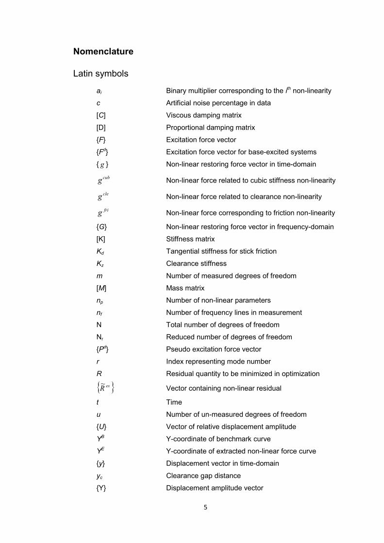
Nomenclature
Latin symbols
ai Binary multiplier corresponding to the ith non-linearity
c Artificial noise percentage in data
[C] Viscous damping matrix
[D] Proportional damping matrix
{F} Excitation force vector
{Fd} Excitation force vector for base-excited systems
{ g } Non-linear restoring force vector in time-domain
cubg Non-linear force related to cubic stiffness non-linearity
cleg Non-linear force related to clearance non-linearity
frig Non-linear force corresponding to friction non-linearity
{G} Non-linear restoring force vector in frequency-domain
[K] Stiffness matrix
Kd Tangential stiffness for stick friction
Kz Clearance stiffness
m Number of measured degrees of freedom
[M] Mass matrix
np Number of non-linear parameters
nf Number of frequency lines in measurement
N Total number of degrees of freedom
Nr Reduced number of degrees of freedom
{Pd} Pseudo excitation force vector
r Index representing mode number
R Residual quantity to be minimized in optimization
{ }esR~ Vector containing non-linear residual
t Time
u Number of un-measured degrees of freedom
{U} Vector of relative displacement amplitude
YB Y-coordinate of benchmark curve
YE Y-coordinate of extracted non-linear force curve
{y} Displacement vector in time-domain
yc Clearance gap distance
{Y} Displacement amplitude vector

6
Greek letters
[ ]α Receptance matrix
[ ]Z Dynamic stiffness matrix
β Coefficient for cubic stiffness non-linearity
ε Error in estimation
η Modal damping ratio
[ ]λ Complex eigenvalues matrix
µ Coefficient of friction
iφ Vector containing ith column from mode shape matrix
[ ]Φ Mode shape matrix
ω Excitation Frequency
ωr Resonance frequency of the rth mode
{ }χ Non-linear modal vector
Subscripts
c Index representing the measurement location close to
non-linear degree of freedom.
e Index representing excitation degree of freedom
m Index representing measured degrees of freedom
max Index representing the maximum value of a variable
Mr Index representing the identified modes
nl Index representing non-linear degree of freedom
u Index representing un-measured degrees of freedom
Ur Index representing the un-identified modes
Superscripts
T Transpose of a matrix
-1 Inverse of a square matrix
+ Pseudo-inverse of a rectangular matrix

7
Abbreviations
1D, 2D,.. One dimensional, two dimensional,...
CFD Computational fluid dynamics
DOF Degree of freedom
DFM Describing function method
FEA Finite element analysis
FEM Finite element method
FFT Fast Fourier transform
FRF Frequency response function
GA Genetic algorithm
HBM Harmonic balance method
HMT Hybrid modal technique
I-HMT Improved hybrid modal technique
LMA Linear modal analysis
MDOFs Multi-degrees of freedom
NMG Non-linear modal grade
NMV Non-linear modal vector
POD Proper orthogonal decomposition
SDOF Single-degree of freedom
SSD Sum of squared distance

8
Contents Abstract ................................................................................................................................. 2
Acknowledgements ............................................................................................................ 3
Nomenclature ....................................................................................................................... 5
Abbreviations ....................................................................................................................... 7
List of Figures .................................................................................................................... 12
List of Tables ...................................................................................................................... 16
Chapter 1 ............................................................................................................................. 18
Introduction ........................................................................................................................ 18
1.1 Background of the problem ..................................................................................... 18
1.2 Non-linear system identification ............................................................................. 19
1.3 The describing function method ............................................................................. 20
1.4 Objectives of the thesis ............................................................................................ 21
1.5 Organization of the thesis ........................................................................................ 22
Chapter 2 ............................................................................................................................. 24
Literature Survey ............................................................................................................... 24
2.1 Introduction ................................................................................................................ 24
2.2 Non-linear system identification ............................................................................. 25
2.2.1 Non-linearity detection ...................................................................................... 27
2.2.2 Non-linearity characterization .......................................................................... 28
2.2.3 Non-linear parameter extraction: Spatial methods ....................................... 29
2.2.4 Non-linear parameters extraction: Modal methods ...................................... 31
2.2.4 Model updating for non-linear systems .......................................................... 33
2.3 Non-linear response prediction............................................................................... 35
2.4 Non-linear structural dynamics: Real life structures ............................................ 39
2.5 Summary of the literature review ........................................................................... 41
Chapter 3 ............................................................................................................................. 43
Non-linearity type identification using a ‘footprint library’ .................................... 43
3.1 Introduction ................................................................................................................ 43
3.2 Generation of non-linear force curves ................................................................... 44
3.3 Footprints of different non-linearities ..................................................................... 46
3.3.1 Cubic stiffness non-linearity ............................................................................. 47
3.3.2 Clearance non-linearity..................................................................................... 48
3.3.3 Friction non-linearity .......................................................................................... 49

9
3.3.4 Combination of different non-linearities ......................................................... 50
3.4 Quantitative comparison using shape-matching algorithm ................................ 55
3.4.1 Generation of footprint curves ......................................................................... 55
3.4.2 Shape-matching algorithm ............................................................................... 57
3.4.3 Universal applicability of the footprint comparison ....................................... 59
3.4.4 Numerical examples ......................................................................................... 64
3.5 Concluding remarks ................................................................................................. 68
Chapter 4 ............................................................................................................................. 71
Spatial method for non-linear parameter identification .......................................... 71
4.1 Introduction ................................................................................................................ 71
4.2 Theoretical formulation ............................................................................................ 72
4.2.1 Non-linearity detection and characterization ................................................. 73
4.2.2 Formulation of the optimization problem ....................................................... 73
4.2.3 Search for the non-linear parameters using a genetic algorithm ............... 75
4.2.4 Use of binary multipliers to improve the efficiency ....................................... 77
4.2.5 Non-linear parameter identification without full measurement set at non-linear DOFs .................................................................................................................. 78
4.3 Numerical examples ................................................................................................. 79
4.3.1 Effect of the number of measurements on parameter estimation .............. 80
4.3.2 Effect of measurement noise on parameter estimation ............................... 83
4.3.3 Effect of binary multipliers on computational efficiency ............................... 85
4.3.4 Effect of the error in the FE model on parameter estimation ...................... 87
4.3.5 Non-linear parameter identification in absence of measurements at non-linear DOFs .................................................................................................................. 89
4.4 Concluding remarks ................................................................................................. 90
Chapter 5 ............................................................................................................................. 92
Non-linear identification using modal models and response models ................ 92
5.1 Introduction ................................................................................................................ 92
5.2 Improved hybrid modal technique (I-HMT) ........................................................... 93
5.2.1 Theoretical formulation ..................................................................................... 93
5.2.2 Quantification of the level of non-linearity ..................................................... 96
5.2.3 Decoupling the non-linear modal vector ........................................................ 97
5.2.4 Comments on the non-linear residual ............................................................ 99
5.2.5 Numerical validation of I-HMT method ......................................................... 102
5.3 FRF-based method ................................................................................................ 107
10
5.3.1 Theoretical formulation ................................................................................... 107
5.3.2 Conditioning of the FRF matrix ..................................................................... 109
5.3.3 Numerical validation of the FRF based method ......................................... 111
5.4 Concluding remarks ............................................................................................... 115
5.4.1 Comments on the I-HMT method ................................................................. 115
5.4.2 Comments on the FRF-based method ......................................................... 115
Chapter 6 ........................................................................................................................... 117
Comparison of non-linear parameter identification methods ............................. 117
6.1 Introduction .............................................................................................................. 117
6.2 Test cases for the comparison ............................................................................. 119
6.3 Pre-processing of the input data .......................................................................... 120
6.3.1 Non-linear displacement measurements on the structure ........................ 120
6.3.2 Input models for different methods ............................................................... 122
6.4 Results of non-linear parameter identification for Case A ................................ 123
6.4 Results of non-linear parameter identification for Case B ................................ 128
6.5 Discussion and concluding remarks .................................................................... 134
Chapter 7 ........................................................................................................................... 137
Experimental investigation of non-linearities in MACE structure ...................... 137
7.1 Introduction .............................................................................................................. 137
7.1.1 Choice of the structure ................................................................................... 137
7.1.2 Description of joints in Sub-assembly 3 ....................................................... 138
7.1.3 Objectives of the exercise .............................................................................. 139
7.2 Validation of the FE models .................................................................................. 140
7.3 Detection of non-linear behaviour ........................................................................ 144
7.3.1 Problem of force-drop near resonance ........................................................ 144
7.3.2 Non-linearity detection with constant-force step-sine tests ...................... 147
7.4 Characterization of the non-linearity .................................................................... 150
7.4.1 Identifying the location non-linearity ............................................................. 151
7.4.2 Identifying the type of non-linearity ............................................................... 152
7.4.3 Estimation of non-linear parameters ............................................................ 156
7.5 Concluding remarks ............................................................................................... 160
Chapter 8 ........................................................................................................................... 161
Non-linear parameter identification for base-excited structures ....................... 161
8.1 Introduction .............................................................................................................. 161

11
8.2 Theoretical formulation .......................................................................................... 162
8.3 Implementation of the method .............................................................................. 164
8.4 Illustration of the method ....................................................................................... 165
8.4.1 Stage 1: Extraction of pseudo excitation force vector (Pd)........................ 166
8.4.2 Stage 2: Obtaining the non-linear restoring force ...................................... 168
8.4.3 Stage 3: Estimation of the non-linear parameters ...................................... 168
8.4.4 Performance in the presence of experimental noise ................................. 170
8.5 Concluding remarks ............................................................................................... 170
Chapter 9 ........................................................................................................................... 172
Conclusions and future work....................................................................................... 172
9.1 Conclusions of the research work ........................................................................ 172
9.1.1 Type characterization using footprints ......................................................... 172
9.1.2 Genetic algorithm optimization ...................................................................... 173
9.1.3 On the choice of the model for the underlying linear system ................... 173
9.1.4 Experimental investigation of non-linear behaviour ................................... 174
9.1.5 Identification method for base-excited structures ....................................... 175
9.3 Contributions and publications of the thesis ....................................................... 176
9.4 Suggestions for future work .................................................................................. 176
References ........................................................................................................................ 178
Appendix A ....................................................................................................................... 185
System used for the generation of footprint library ...................................................... 185
Appendix B ....................................................................................................................... 186
Structures used for the validation ................................................................................... 186
Validation Structure-1: Cantilever beam .................................................................... 186
Validation Structure-2 Cantilever plate ...................................................................... 186
Validation Structure-3 Pyramid ................................................................................... 188
Appendix C ....................................................................................................................... 190
Details of ‘1203 structure’ ................................................................................................ 190
Appendix D ....................................................................................................................... 191
MACE structure details and repeatability test results .................................................. 191
D.1. Material properties and the FE model mesh information ................................ 191
D.2. Repeatability tests for non-linear measurements ............................................ 191
12
List of Figures 1.1 Difference between linear and non-linear systems 20
1.2 Single HBM approximation of clearance non-linearity 21
1.3 Thesis contents 22
2.1 Research in non-linear structural dynamics 25
2.2 Benchmark structures for European COST F3 39
2.3 Experimental setup used by Ferreira and Elizalde 40
3.1 The two DOF system used to generate footprint library 45
3.2 A typical frequency response curve for a non-linear system 46
3.3 Non-linear force: Cubic stiffness non-linearity (hardening) 47
3.4 Non-linear force: Cubic stiffness non-linearity (softening) 47
3.5 Non-linear force: Clearance non-linearity 48
3.6 Comparison of cubic stiffness and clearance non-linearity 48
3.7 Non-linear force: Friction with pure slip 49
3.8 Non-linear force: Friction with pure stick 49
3.9 Non-linear force: Friction with stick and slip 50
3.10 Non-linear force: cubic stiffness and clearance 51
3.11 Non-linear force: Cubic stiffness and friction 51
3.12 Non-linear force: Clearance and friction 51
3.13 Non-linear force: Cubic stiffness, clearance and friction 52
3.14 Footprint library: magnitude plots for non-linear force 53
3.15 Footprint library: Nyquist plots for non-linear force 54
3.16 Normalized footprint for cubic stiffness 55
3.17 Library of normalized footprints for quantitative comparison 57
3.18 Comparison steps for shape-matching 58
3.19 Flowchart for shape-matching algorithm 59
3.20 Numerical experiments: cubic stiffness non-linearity 60
3.21 Numerical experiments: clearance non-linearity 60
3.22 Numerical experiments: friction 61

13
3.23 Numerical experiments: clearance and friction 62
3.24 Comparison with finer footprints for cubic stiffness and friction 63
3.25 Non-linear force for case 1 (cubic stiffness) 65
3.26 Quantitative comparison for Case 1 65
3.27 Non-linear force for Case 2 (friction) 66
3.28 Quantitative comparison for Case 2 66
3.29 Non-linear force for Case 3 (cubic stiffness + friction) 67
3.30 Quantitative comparison for Case 3 67
3.31 Quantitative comparison for Case 3 with 7.5% noise 69
4.1 Flowchart of the genetic algorithm optimization 77
4.2 Comparison of linear and non-linear responses 80
4.3 Identification of non-linearity location (Case A) 81
4.4 Non-linearity characterization (Case A) 82
4.5 Displacement response with 5% random noise 84
4.6 Comparison of the extracted and regenerated non-linear force 85
4.7 Performance of binary multipliers: fittest string fitness 86
4.8 Performance of binary multipliers: Average fitness 87
4.9 Accumulated non-linear force plot 88
4.10 Non-linear force at un-measured DOFs 89
5.1 Half power method to calculate the average NMV 97
5.2 Flow chart for the improved hybrid modal method 100
5.3 Comparison of linear and non-linear residual for a typical case 101
5.4 Non-linear residuals with different number of modes in the range 101
5.5 Comparison of linear and non-linear response for clearance non-
linearity
102
5.6 Details of the measured locations 103
5.7 Extracted non-linear modal vector for the first mode 104
5.8 Zoomed-in view of NMV near the first resonance 105
5.9 Non-linear modal grades for the modes in the measurement range 105
5.10 Variation of the condition number of the FRF matrix 110
5.11 Effect of measurement locations on the condition number 110
5.12 Linear and non-linear response at the excitation DOF 111
5.13 Details of the measurement locations for three cases 112
5.14 Non-linear force for Cases A and B 112
5.15 Extraction of the non-linear force for Case C 113
5.16 Comparison of the accurate response and the regenerated 114

14
response for the FRF-based method predictions
6.1 CAD and FE models ‘1203 structure’ 119
6.2 Depiction of two test cases used for comparison study 120
6.3 Measurement locations on the 1203 structure 121
6.4 Non-linear response for Case A (cubic stiffness non-linearity) 121
6.5 Non-linear response for Case B (clearance non-linearity) 122
6.6 Identification of the location of non-linearity for Case A 124
6.7 Non-linear force at the non-linear DOF for Case A 124
6.8 Non-linear modal vector plotted for Case A 125
6.9 Non-linear modal grade (NMG) plot for Case A 125
6.10 Non-linear force plot with 5% measurement noise for Case A 126
6.11 NMV for the 2nd mode plotted for Case A with noise 127
6.12 Accumulated non-linear force at measured DOFs for Case B 129
6.13 Accumulated non-linear force mapped on measurement locations 130
6.14 NMV and NMG plots for Case B 130
6.15 Comparison of non-linear force for Method 1 131
6.16 Comparison of non-linear force for Method 3 132
6.17 Depiction of calculation of errors for Case B 133
7.1 Computer-generated drawing of the MACE structure 138
7.2 Schematic of Sub-assembly 3 139
7.3 FE models of the individual components 140
7.4 Mode shapes of the assembled structure via FEA 142
7.5a Point FRF plot for the assembled structure (hammer tests) 142
7.5b Overlaid FRFs for the EMA on the assembled structure 143
7.6 Force drop near resonance for the MACE sub-assembly 145
7.7 Overlaid FRFs at different excitation levels without force-control 145
7.8 Flow chart for the force-control algorithm 146
7.9 Experimental setup for non-linear step-sine testing 147
7.10 Overlaid accelerance at different excitation levels with force-
control
148
7.11 Nyquist plots for accelerance at different excitation levels 148
7.12 Presence of higher-harmonics in the response at 10N force level 149
7.13 Contribution of the higher harmonics at different excitation levels 150
7.14 Measurement locations on the MACE sub-assembly 151
7.15 Accumulated non-linear force at the measurement locations 151
7.16 Variation of the resonance amplitude for the first mode 152

15
7.17 Variation of the resonance frequency of the first mode 153
7.18 Inverse FRF plots at excitation force level = 5N 153
7.19 Non-linear force at locations A1 and A4 154
7.20 Non-linear force at A4 against displacement at A4 155
7.21 Comparison of non-linear force extracted using different methods 155
7.22 Comparison of the extracted non-linear force with footprint library 156
7.23 Regenerated non-linear forces with parametric and non-
parametric models
158
7.24 Regeneration of response using non-parametric model 158
7.25 Regeneration of response using parametric model 159
8.1 Flowchart of the proposed method 165
8.2 Schematic of Validation structure-3 166
8.3 Overlaid FRFs of the underlying linear structure 167
8.4 Pseudo excitation force at measured DOFs 167
8.5 Comparison of linear and non-linear responses at low and high
acceleration input
168
8.6 Identification of non-linearity location 169
8.7 Non-linear force at the non-linear DOF 169
A1 2 DOF system used to generate footprint library 185
B1 Validation structure- 1: Cantilever beam 186
B2 Validation structure- 2: Cantilever plate 187
B3 Mode shapes for validation structure-2 188
B4 Engineering drawing of validation structure-3 189
C1 Engineering drawing of 1203 structure 190
D1 Repeatability test results at force level 0.5N 192
D2 Repeatability test results at force level 3N 192
D3 Repeatability test results at force level 5N 192

16
List of Tables 3.1 Expressions for non-linear restoring force 56
3.2 Summary of non-linear parameters used for validation 64
3.3 Summary of the quantitative comparison 68
3.4 Summary of the quantitative comparison with noise 69
4.1 Description of measured DOFs 81
4.2 Parameters used in the GA 82
4.3 Summary of results for parameter estimation 83
4.4 Results of parameter estimation in presence of noise 84
4.5 Performance of binary multipliers 86
4.6 Effects of the erroneous FE model 88
4.7 Case description for non-linear parameter identification in absence of
the measurement at non-linear DOFs
89
5.1 Results of parameter estimation for different cases using I-HMT
method
106
5.2 Summary of the parameter identification results using FRF-based
method
113
6.1 Details of the three methods compared 118
6.2 Summary of non-linear parameters used for the two cases 120
6.3 Results of parameter estimation for clean measurement data with
accurate input models
126
6.4 Estimated non-linear parameter with noise for Case A 127
6.5 Estimated non-linear parameter with erroneous input models for
Case A
128
6.6 Estimated parameters with accurate input models and without
measurement noise for Case B
131
6.7 Summary of estimated non-linear parameters for cases of noisy data
and erroneous input models for Case B
132
6.8 Summary of errors in resonance response and resonance frequency 133
6.9 Quantitative comparison of the three methods 136
7.1 Description of joints in Sub-assembly 3 139
17
7.2 Correlation of modal properties for individual components 141
7.3 Comparison of the modal properties of the assembled structure 143
7.4 Estimated non-linear parameters with parametric and non-parametric
models
157
7.5 Comparison of errors in the regenerated response 159
8.1 Estimated parameters with and without noise 170
A1 Non-linear parameters for different non-linearities 185
B1 Linear natural frequencies for validation structure-2 187
B2 Material properties for beams in validation structure-3 188
C1 Natural frequencies of the underlying linear structure 190
D1 Details of material properties and FE model mesh 191

18
Chapter 1
Introduction This chapter presents a brief introduction to the subject of non-linear structural
dynamics. The importance of the research in this area and its relevance to industry
are stated. The terminologies specific to non-linear structural dynamics, which are
frequently used in the thesis, are discussed to facilitate the reading of the thesis.
The statement of the problem, as addressed in this thesis, is presented. In the last
section, the structure of the thesis and the relationships between different chapters
are presented in order to give an overview of the thesis.
1.1 Background of the problem
In recent years, continuous attempts have been made to shorten the product design
cycle. To survive in a competitive market, it is of paramount interest to
manufacturers to reduce the cost and the time associated with the experimental
validation of prototypes. This need, coupled with the availability of computational
resources and numerical tools like FEA and CFD, has increased the use of
computer simulations to predict structural behaviour. For linear systems, the
dynamic behaviour of a system can be accurately predicted using numerical tools
like FEA. But in the real world, non-linearity is omnipresent and linear behaviour is
the exception. As engineers are seeking to design lighter, flexible, faster, and more
efficient products, the designs are shifting more in the non-linear regime. On the
other hand, there are very few established and validated methods for predicting the
response of non-linear systems.
What is non-linearity? Non-linearity is quite a broad term which may possess different meanings in
contexts of different engineering disciplines. From structural dynamicist’s
perspective, non-linearity is something which causes the system to violate the
principle of homogeneity. Mathematically, non-linear systems can be represented by

19
a set of differential equations with non-linear terms. The resonance frequencies and
mode shapes of such systems are functions of the operating conditions [1].
Various domains of engineering, like aerospace, automobile, machine tool
industry, spacecraft technology, civil and structural engineering, encounter non-
linear systems in one form or the other. Some common occurrences of non-
linearities in engineering are: (i) friction induced non-linearities in bolted joints, (ii)
backlash and clearance non-linearities in control surfaces of aero-structures, (iii)
polynomial stiffness non-linearities observed in the engine-wing connection of an
airplane, (iv) non-linearities demonstrated by engineering materials like composites,
plastics, and viscoelastic materials.
As discussed in [2], non-linearities arising from various sources can easily
invalidate the results of simulations based on linearity. It has been shown in [3-5],
either experimentally or through simulations, that the dynamic behaviour of strongly
non-linear systems can be significantly different than that of their linear
counterparts. Thus, it has become important to accurately predict the behaviour of
non-linear systems.
To predict the behaviour of non-linear systems, it is necessary to include the
corresponding non-linear elements into the numerical/mathematical models which
describe those systems. The parameters of such non-linear elements are case
specific, and must usually be identified through experimental route for the case of
interest. The process of identifying the parameters of the mathematical model of a
system is known as system identification
1.2 Non-linear system identification
Linear system identification, which attempts to determine mathematical models of
linear dynamic systems from vibration measurements, is an established area of
study. The tools like modal testing and analysis [6, 7] are available off-the-shelf for
linear system identification. For linear systems, the transfer function, relating the
input of the system to its output, remains constant at all excitation levels. Thus, the
mathematic model obtained through the identification at one operating point can
later be used for prediction at some other operating point. For non-linear systems, it
is difficult to obtain a universal mathematical model of the system by performing the
system identification only at a single excitation level. A model obtained at a given
operating condition can, at best, provide the equivalent linear system at that point.
Figure 1.1 depicts the difference between linear and non-linear systems seen from a

20
system identification perspective. It can be seen from the figure that for non-linear
systems, the transfer function is not independent of the input.
Figure 1.1 Difference between linear and non-linear systems
Thus, the identification of non-linear systems differs from the conventional linear
system identification. The scope of non-linear system identification in this thesis is
confined to detecting the non-linear behaviour, identifying its location and type, and
estimating its parameters as inputs to the models which describe the non-linear
system.
1.3 The describing function method
The describing function method (DFM), which finds its origin in control systems
engineering [8], is a very popular method to predict the response of non-linear
systems. The method seeks to find an input-output relationship for non-linear
systems by assuming approximate functions, called describing functions, to
describe the behaviour of non-linear elements in the system. The coefficients of
these describing functions are obtained by matching the restoring force in the
system.
For systems with sinusoidal input, the coefficients of describing functions
can be derived by using a method which is popularly known as the harmonic
balance method (HBM). In this case, the non-linear part of the restoring force is
assumed to be periodic, so that it can be expressed as a Fourier series. The Fourier
series may be truncated to include only the fundamental harmonics, leading to a
technique called single-harmonic balance method. As the number of harmonics in
the analysis is increased, a better approximation can be achieved. In the harmonic
balance method, the Fourier coefficients are obtained by computing the area under
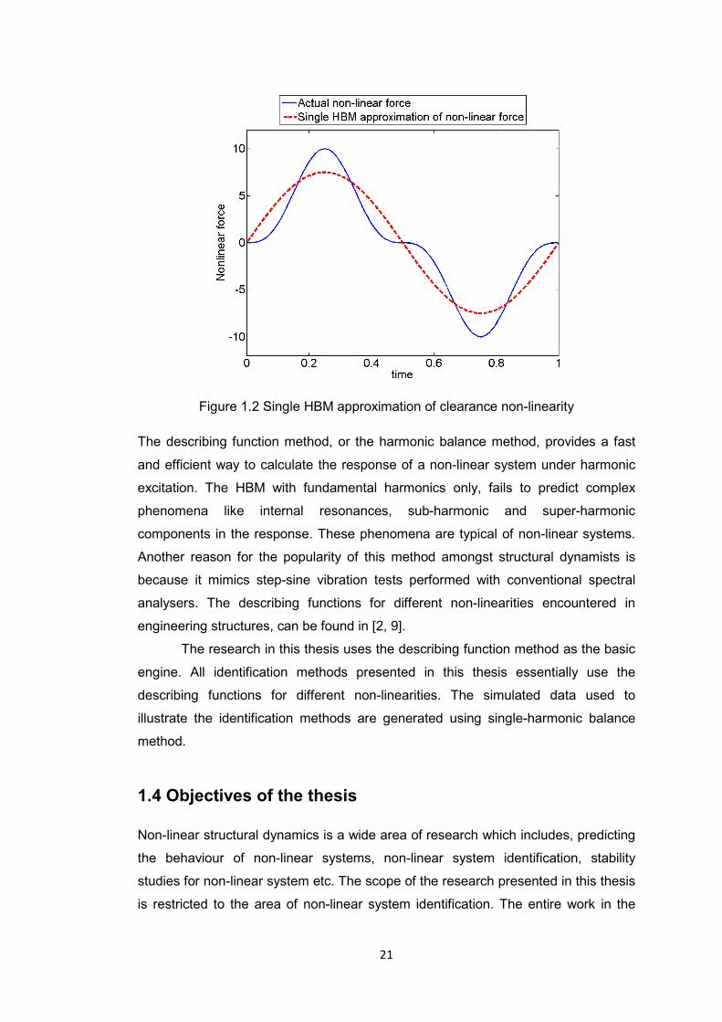
the non-linear force curve for one complete cycle. Figure 1.2 shows, for clearance
non-linearity, a comparison of actual non-linear force and the approximated non-
linear force with single harmonic balance method.
21
Figure 1.2 Single HBM approximation of clearance non-linearity
The describing function method, or the harmonic balance method, provides a fast
and efficient way to calculate the response of a non-linear system under harmonic
excitation. The HBM with fundamental harmonics only, fails to predict complex
phenomena like internal resonances, sub-harmonic and super-harmonic
components in the response. These phenomena are typical of non-linear systems.
Another reason for the popularity of this method amongst structural dynamists is
because it mimics step-sine vibration tests performed with conventional spectral
analysers. The describing functions for different non-linearities encountered in
engineering structures, can be found in [2, 9].
The research in this thesis uses the describing function method as the basic
engine. All identification methods presented in this thesis essentially use the
describing functions for different non-linearities. The simulated data used to
illustrate the identification methods are generated using single-harmonic balance
method.
1.4 Objectives of the thesis
Non-linear structural dynamics is a wide area of research which includes, predicting
the behaviour of non-linear systems, non-linear system identification, stability
studies for non-linear system etc. The scope of the research presented in this thesis
is restricted to the area of non-linear system identification. The entire work in the
22
thesis is based on the already established theory of describing functions (DFM). The
statement of the problem, which is attempted in this thesis, is given as follows:
“To propose and illustrate different strategies for non-linear system identification
which suit complex and realistic engineering systems. The realm of non-linear
system identification would encompass different sub-activities like detection of non-
linearities in the system, identification of the type of non-linearity, and estimation of
the non-linear parameters.”
1.5 Organization of the thesis
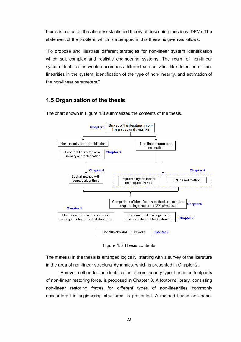
The chart shown in Figure 1.3 summarizes the contents of the thesis.
Figure 1.3 Thesis contents
The material in the thesis is arranged logically, starting with a survey of the literature
in the area of non-linear structural dynamics, which is presented in Chapter 2.
A novel method for the identification of non-linearity type, based on footprints
of non-linear restoring force, is proposed in Chapter 3. A footprint library, consisting
non-linear restoring forces for different types of non-linearities commonly
encountered in engineering structures, is presented. A method based on shape-

23
matching algorithm for quantitative matching of non-linear force curves is also
presented.
After the non-linearity type identification, the next stage is the non-linear
parameter estimation. A method for non-linear parameter estimation, which uses the
FE model of the underlying linear structure, is proposed in Chapter 4. The method
extracts the non-linear parameters via genetic algorithm optimization. The method is
illustrated on a simple cantilever beam case.
An accurate FE model might not be available in some practical cases. The
methods which bypass the requirement of the updated FE model are presented in
Chapter 5. Two proposed methods use the modal model and the response model of
the underlying linear structure respectively. The methods are exemplified using
simulated data for a cantilever plate.
The methods presented in earlier chapters have their own advantages and
disadvantages. These are compared on common ground by using simulated data
for a relatively complex and realistic engineering structure, the so-called 1203
structure. The results of the comparison are presented in Chapter 6.
Chapter 7 presents an experimental investigation of non-linearities in the so-
called MACE structure, the structure with different joints and connections
contributing towards non-linear behaviour. A complete process of non-linear
identification is attempted on this structure with experimental data.
Many times, for large structures, vibration tests are performed with the
structure mounted on a shaker table, and controlling the acceleration input to the
structure. Since the force input is not measured in such cases, conventional non-
linearity identification methods cannot be applied. Chapter 8 presents a novel
strategy of non-linear parameter estimation for the case of base-excited structures.
In the last chapter of the thesis, Chapter 9, the main contributions of the
research are summarized. Some concluding remarks on the research and
suggestions for future work on this topic are presented.

24
Chapter 2
Literature Survey This chapter presents a survey of the literature in the area of non-linear structural
dynamics. The survey presented is not all-encompassing but more specific to the
topics related to the thesis. The literature which helped the author to define the
research problem, and which is closely related to the research presented in the
thesis is dealt with in detail. For an exhaustive survey of the literature, the reader is
directed to the excellent review articles [10-13] published on this topic. For an
introduction to non-linear structural dynamics in general, the books by Nayfeh and
Mook [14] and Worden and Tomlinson [2] serve as a good starting point. The review
in this chapter is organized methodologically, and within the methodologies, the
work is arranged in chronological order.
2.1 Introduction
From a structural dynamicist’s perspective, non-linearity can be defined as the
deviation of a structure from linear behaviour. The non-linearity is manifested in the
form of amplitude-dependent vibration properties, complex phenomena like mode
localization, bifurcations, internal resonances, presence of sub-harmonic and super-
harmonic components in the response, jump phenomenon etc.
The research in the area of non-linear structural dynamics started more than
four decades ago. The research later gained the popularity and wide acceptance
when it was understood that all engineering structures are non-linear to some
extent. The research progressed in two fundamental branches: (i) non-linear system
identification and, (ii) prediction of non-linear response under different operating
conditions. Different methodologies emerged within these two fundamental
branches. A chart showing the span of the research in this area is presented in
Figure 2.1. The different methods proposed for identification and modelling of non-

25
linearities are presented in separate sections. The last section presents the
literature on application of these methods to complex engineering structures.
Figure 2.1 Research in non-linear structural dynamics
2.2 Non-linear system identification
The main goal of any system identification method is to find parameters of a
mathematical model representing a physical system, by making use of the input and
output data describing the excitation and response of the system. For linear
structural dynamics, there are three popular representations to describe the physical
system: (i) the spatial model, (ii) the modal model, and (iii) the response model. The
modal model is the most compact form which is easily obtainable through
experimental route [6]. Thus, most of the linear system identification methods
extract the parameters of the modal model of the system, a process which is
popularly known as linear modal analysis (LMA).
For a non-linear system, the properties like linear modal superposition,
reciprocity, homogeneity which form the back-bone of LMA theory are not valid.
Thus, non-linear system identification is more involved than just to extract the
parameters for the modal model of the system. Some basic treatment and practical
26
advice on handling the non-linear system is presented in a primer on modal analysis
published by Dynamic Testing Agency [15].
There are three stages of non-linear system identification, (i) Non-linearity
detection, (ii) Non-linearity characterization, and (iii) Non-linear parameter
extraction. In the first stage, the presence of the non-linearity is detected from the
experimental measurements. In the second stage, the type and form of non-linearity
is identified and in the last stage, the corresponding non-linear parameters are
identified [11].
There are several ways to classify the literature on non-linear system
identification. One way of classification is based on how the non-linear system
identification problem is perceived. It can be perceived merely as a parameter
estimation problem in which the non-linear parameters are extracted making use of
the model of the underlying linear system1. It can also be perceived as non-linear
modal analysis problem in which the linear modal analysis theory is extended to the
non-linear systems. In this approach, the non-linearities are either described in
modal coordinates, or they are presented as a variation in modal properties like
natural frequency, mode shapes, and damping. Another way of perceiving non-
linear system identification is as a problem of model updating. In this approach, the
linear model of the structure is refined/ corrected in order to match the experimental
measurements. This is achieved either by modifying the system properties or by
adding some special elements which may or may not have physical significance.
Another classification of the parameter estimation methods is based on the
nature of model that is fitted in the data. The methods can be classified into: (i)
parametric and (ii) non-parametric methods. In parametric methods, the model has
some physical meaning. For example, to describe a clearance non-linearity, the
parameters identified are the clearance distance and the normal stiffness. Naturally,
the parametric methods give insight into the nature and the physics of non-linear
behaviour, but the highly individualistic nature of non-linearities makes it difficult to
find a parametric model to suit different non-linearities observed in engineering
structures. In non-parametric identification, the extracted parameters do not
necessarily have any physical meaning.
It is relatively easy to extract a non-parametric model to fit into the data, but
the extrapolation capacity of non-parametric models cannot be guaranteed. The
non-parametric models, being non-physical, are not universal. In many cases they
yield poor predictions when stretched outside their working range. Black box
1 Most of the times, for practical structures, it’s the FE model
27
methods form a significant group in non-parametric methods. These methods
sometimes use non-conventional techniques like neural networks, fuzzy logic etc. to
model the input-output relationship for the non-linear systems. It is not intended to
discuss these methods, and a detailed review of black box methods can be found in
[16, 17].
The literature associated with non-linearity detection, characterization and
different approaches for non-linear parameter estimation is presented separately in
the following sections.
2.2.1 Non-linearity detection
The first stage in non-linear system identification is to detect if there is any non-
linearity in the system. Non-linearity detection is a mature area of research with
many established methods available in the literature. A summary of non-linearity
detection techniques and their comparison is presented in [12, 18, 19]. The methods
are compared on the basis of different criteria like measurement time, computation
time, range of application, subjectivity involved etc.
Mostly, the presence of non-linearity is detected by verifying the fundamental
principles of linear systems like linear superposition or reciprocity. The distortion of
Nyquist plot and frequency response functions (FRFs) also indicate the presence of
non-linearity as explained in [2, 6]. The first-order FRFs obtained using the
conventional vibration testing are primarily used to validate these properties.
He and Ewins [20] suggested the use of inverse FRF to detect the presence
of non-linearity. For a non-linear system, real and imaginary parts of FRF, plotted
against frequency-squared and frequency respectively, deviate from a straight line
indicating the presence of non-linearity. A similar method based on mapping of
stiffness and damping at each frequency value is suggested by Mertens et al. [21].
This method, which is limited to single degree of freedom (SDOF) systems, detects
the presence of non-linearity in the system if any variation in stiffness or damping is
observed. Tomlinson [22] proposed the use of Hilbert transform to detect the non-
linearity. Hilbert transform of a complex FRF of a linear system is same as the
original FRF. For non-linear system the transform deviates from the original FRF,
the deviation being utilized to detect the presence of non-linearity.
For linear systems with single harmonic excitation, the response is harmonic
with the same frequency. For non-linear systems, the response is expected to
contain higher harmonics. The higher harmonics in the response can be used to
detect the non-linearity. Wyckaert [23] proposed a term called harmonic detection

28
function (HDF) to quantify the presence of higher harmonics at each frequency. The
HDF is defined as the ratio of the energy associated with higher harmonics at a
frequency to the total energy in the response at that frequency. Chong and Imregun
[24] showed that a lack of orthogonality between the mode shape vectors and the
reciprocal modal vectors (RMV), obtained from measured frequency response
functions, can also indicate the non-linear behaviour.
To decide on whether to use a linearized model or to build a non-linear
model of a system, it is essential to know the extent of non-linearity in the system.
Though the above methods work well to detect the presence of non-linearity, they
provide little information about the extent of non-linearity. Surprisingly, there are
very few attempts to quantify the level of non-linearity in the structure.
Kim and Park [25] proposed a term called ‘non-casual power ratio’ (NPR) to
gauge the extent of non-linear contamination. They used inverse Fourier transform
on the FRF to get a time-domain signal. NPR is defined as the ratio of non-casual
power to the total power in the signal. It is claimed that as the non-linear effects
dominate, the non-causal power in the signal increases. NPR varies from 0 to 1 with
increasing non-linear contribution.
Elizalde [26] coined a term called non-linear modal grade to quantify the
non-linear contamination of each mode. He used thresholds based on engineering
judgments to define 3 ranges: weakly non-linear, moderately non-linear and strongly
non-linear for each mode. Depending on the non-linear grade for a mode, it can be
decided whether to include that mode in non-linear analysis.
2.2.2 Non-linearity characterization
Non-linearity characterization, as defined in [11], is to find the location, the type, and
the functional form of all non-linearities in the system. Non-linearity characterization
is an important step in a bigger goal of non-linear system identification. Many non-
linear parameter extraction methods in the literature assume that the
characterization is completed in advance.
For simple structures with few joints and connections, the spatial location of
non-linearity can be guessed merely by looking at the structure. For complex
structures with many connections, it becomes necessary to locate the connections
which are contributing towards the non-linear behaviour of the structure. Al-Hadid
and Wright [27] proposed a method based on force-state mapping to locate the non-
linear DOF. The method is developed for lumped-parameter system and it is difficult
to implement for a continuous system. Elizalde [26] and Ozer et al. [28] used non-
29
linear restoring force at each DOF as an indication of non-linearity. A non-zero value
of non-linear restoring force at any DOF signifies the non-linearity at that DOF. The
methods are potentially applicable for engineering structures and work well with FE
models.
Some of the methods stated for non-linearity detection in the earlier section
can be extended to find the type of non-linearity. The inverse FRF method proposed
by He and Ewins [20] classifies the non-linearity broadly into stiffness type and
damping type. A deviation of Hilbert transform of an FRF from the original FRF is
characteristic of the type of non-linearity as shown by Tomlinson [22]. He presented
Hilbert transform of simulated FRFs for different types on non-linearities. A restoring
force surface technique (RFS), proposed by Masri and Caughey [29] can be used to
characterize the non-linearity type. In this method, the restoring force due to
stiffness and damping is plotted against the system variables to form a surface. The
restoring surface thus formed is unique to the type of non-linearity in the system.
The subjective observation of the distortions in FRF is often used to
characterize the type of non-linearity. Adams and Allemang [30] proposed a method
for characterization based on the distortions in the FRF. They modelled the non-
linear system as a closed loop linear system with non-linear elements providing
internal feedback. The modulation of the FRF due to this feedback is used to
characterize the non-linearity type. Tanrikulu and Ozguven [31] used the non-
linearity matrix to characterize the type of non-linearity. The non-linear restoring
force is separated into a matrix and a non-linear response vector. The matrix
contains non-linearities in the form of describing functions. Later, a similar approach
is implemented by Elizalde [26].
Even though the non-linearity characterization forms an important and
sometimes rather essential step in non-linear system identification, there is lack of
well established methods to handle complex engineering structures. Still, most of
the times, a subjective judgment is made about the location and type of non-
linearity.
2.2.3 Non-linear parameter extraction: Spatial methods
Non-linear system modelling techniques use mathematical models to describe the
physical phenomena. Non-linear parameter extraction methods essentially extract
the values of the parameters used in these models using experimental
measurements.
30
Amongst the non-parametric spatial methods, which are mostly in time-
domain, a pioneering work is done by Marsi and Caughey [29]. They proposed a
method called restoring force surface (RFS) in which the restoring force is plotted
against instantaneous values of displacement and velocity in phase plane. The
surface is then approximated by the double Chebyshev polynomials to identify the
non-linear parameters. The original method, which was developed for an SDOF
system, was later extended by different researchers to suit the multi degrees of
freedom (MDOFs) systems [11]. Leontaritis and Billings [32] proposed another
method in time domain non-parametric class called non-linear auto regressive
moving average with exogenous inputs (NARMAX). This is an extension of ARMAX
method [33] used in the linear system identification. The method is versatile in its
use, but for complex engineering structures, the computational burden of the
method can be significant.
In frequency domain, most of the methods use first-order frequency
response functions. There are some methods as listed in [11] which make use of
higher order FRFs and Volterra series, but their use is restricted due to difficulties in
measuring the higher order FRFs for engineering structures. The use of harmonic
balance method [34, 35] and describing functions is popular for parametric
description of non-linearities. The basic assumption in this approach is that for
harmonic excitation, the non-linear restoring force is periodic, and it can be
represented as a summation of different harmonics. Single and multi-harmonic
describing functions for different non-linearities can be formulated and parametric
identification can be performed by fitting the extracted non-linear restoring force in
the describing functions. A list of describing functions for common structural non-
linear elements is presented by Tomlinson and Worden [2]. A more specific list for
the non-linear elements relevant to aerospace industry is published by Goge et al. in
[9].
Tanrikulu and Ozguven [31] proposed a method which separates the non-
linear restoring force into a non-linear response vector and a non-linearity matrix.
This non-linearity matrix is formulated using the describing functions. The method,
originally restricted to grounded non-linearities, is extended for more general use by
Ozer et al. [28]. A similar approach is followed by Elizalde [36] to propose a method
called explicit formulation (EF). The method, which is originally developed for non-
linear response prediction, can be used in reverse path for non-linear identification.
The method is tested on simulated data for a plate with cubic stiffness non-
linearities at multiple locations.

31
The above methods make use of an accurate underlying linear spatial
model, which is not easy to obtain for a complex engineering structure. Elizalde [26]
addressed this difficulty partially by proposing a hybrid method for identification
called reverse hybrid modal technique (R-HMT). This method uses the modal
description for the underlying linear structure and spatial description for the non-
linear elements.
Amongst the other frequency domain methods, Richard and Singh [37]
proposed a method for non-linear identification based on first order FRFs. The
method is called conditioned reverse path (CRP) with a central theme to separate
the non-linear distortions from the measured FRFs using spectral conditioning. The
underlying linear model and non-linearities are then identified independently. The
method has a potential to identify complex MDOFs systems excited using Gaussian
random excitations. The method assumes that the location and the type of non-
linearity are known a priori, and measurements are available at all non-linear DOFs
This puts considerable limitation on its use for real-life engineering structures.
Another frequency domain method, similar to CRP is non-linear identification
through feedback of the output (NIFO) proposed by Adams and Allemang [38]. The
identification for underlying linear system and non-linear components is carried out
simultaneously. In this method, non-linear forces are modelled as an internal
feedback into a closed loop linear system. This method does not guarantee
conditioning as CRP, but its compact formulation makes it simpler to implement.
Most of the parametric methods in spatial domain suffer from some common
limitations like: the need to measure the response at all non-linear DOFs and the
need to know in advance the location and the types of non-linearities present in the
structure. The modal approach, which is discussed in next section, can sometimes
be used to overcome these limitations.
2.2.4 Non-linear parameters extraction: Modal methods
For a linear system, a modal model is very compact way of representing a system
for accurate response predictions. The fundamental properties like natural
frequencies, damping ratios, and mode shapes, for linear systems, are independent
of the excitation amplitude. The modal model is easily obtainable through
experimental route using modal testing and modal analysis [6, 7] which is an
established area of study.
Rosenberg [39] in 1960s proposed a concept of normal modes for non-linear
systems. He defined non-linear normal modes (NNMs) as a motion in which all

32
points of the system vibrate with same phase. This is purely an extension of the
definition of normal modes used for linear system. There was not much research in
this area until Vakakis [40, 41], Shaw and Pierre [42, 43] independently started to
work on it. Shaw and Pierre generalized Rosenberg’s definition by proposing a
concept of invariant manifold. They represented NNMs as surfaces in a phase
plane. NNMs theory is based on a thorough mathematical framework and it
successfully explains distinctive non-linear phenomena like internal resonance,
localization of mode shapes, mode bifurcations, frequency-energy dependence etc.
The very mathematics that enables the theory to describe all complex physics
makes it difficult to use in everyday engineering applications. Recently, Gilbert [44]
proposed a method to synthesize measured non-linear FRFs using a concept of
non-linear normal modes. Peeters et al. [45, 46] proposed numerical techniques for
computation of NNMs based on continuation of periodic solutions. The method
makes use of system matrices to obtain NNMs for the system and it is potentially
suitable for complex engineering structures. It would be interesting to see if the
NNMs theory establishes itself a place in practical engineering applications in the
near future.
Without sticking strictly to the NNMs, many researchers attempted to
express non-linear identification problem in modal domain. He and Ewins [20, 47]
proposed a method based on inverse receptance to find the variation of natural
frequency2 and damping factor for each mode. The method is based on SDOF
assumption and neglects the contribution from the other modes. The method also
assumes that mode shapes of non-linear system are same as the mode shapes of
the underlying linear system.
For free vibration response, Feldman [48] developed a method called
FREEVIB based on Hilbert transform in time domain to obtain the variation of
natural frequency and damping with respect to the amplitude of vibration. He
observed that the dissipative (damping) and elastic (stiffness) non-linearities have
an effect on the instantaneous natural frequency and damping parameters. From
the free vibration response for different non-linearities, he obtained variation of
natural frequencies and damping with amplitude of vibration. He proposed another
method, FORCEVIB [49] based on similar principle to analyze the systems with
forced vibrations under narrow and wide band random excitations and slow and fast
sweep sine tests.
2 Or shall we say the resonance frequency
33
Setio et al. [50] proposed a method to extract the non-linear modal
parameters from frequency response tests. They further used the extracted modal
parameters to predict the response of the system at different force levels using non-
linear modal superposition. Chong and Imregun [51] extended the work of Setio et
al. to large MDOF systems. They considered the amplitude dependence of mode
shapes which some of the other researchers had neglected in the past. The method
was checked for the robustness by evaluating the effect of measurement noise and
the sensitivity of the method to inaccurate underlying linear model. In the second
part of the paper [52], they successfully implemented the technique on experimental
data obtained for a laboratory structure with polynomial stiffness characteristics.
Platten et al. [53, 54] proposed the non-linear resonant decay method (NL-
RDM) to identify the non-linearities in modal domain. The method represents
system equations in modal coordinates with the non-linear modal force to
incorporate non-linearities. The force appropriation technique with burst sine
excitation is used to excite a single mode at a time. The extracted non-linear modal
force at each mode is plotted against modal displacement and modal velocity for
form a non-linear restoring surface in modal domain. The surface is fitted to
polynomial to identify the coefficients of the polynomial.
Ozge and Ozguven [55] presented a method to find the variation of modal
properties of non-linear system. They proposed an equivalent linearization of the
system by keeping a constant value of response at the non-linear DOF. A series of
such constant-amplitude tests yields variation of modal properties as a function of
displacement amplitude.
Recently, Elizalde et al. [56] presented a semi-analytical and approximate
approach to determine the variation in modal parameters (natural frequencies and
mode shapes) of a large MDOF system. They used an iterative procedure to extract
the non-linear modal parameters, using the modal model for the underlying linear
system as an initial guess.
2.2.4 Model updating for non-linear systems
The main theme of model updating is to compare the measured and predicted data
for a system, and to refine the model of the system in order to obtain a better
agreement between the two sets of data. Model updating for linear systems
received a good deal of attention for more than last three decades. Different
techniques emerged essentially to update the FE model of the system in light of the
experimental measurements. The reviews of different techniques on this topic can

34
be found in [57, 58]. Friswell and Mottershead [59] wrote a book dedicated to finite
element model updating.
For linear systems, the results from numerical models deviate from the
experimental results mainly because of the uncertainties in boundary conditions,
material properties, and to some extent, the physical dimensions. These parameters
are generally chosen for updating the numerical model. As a basis of comparison,
different quantities can be used. The most popular are either the modal properties
like natural frequencies and mode shapes, or the response of the system either in
frequency domain (FRFs) or time domain.
For a non-linear system, modal properties are not constant. The resonance
frequencies and mode shapes are dependent on the response amplitude at non-
linear DOFs, and, indirectly on the excitation level. If the modal properties
determined at some excitation level are used as a basis of comparison in model
updating; then the updated model would result in a linearized model of the system
at that excitation level. This model can seldom be used to accurately predict the
response of the system at some other excitation level. If the type of the excitation
and its range remains more or less constant for the application, the linearized
updated model can be sufficient.
The linearized updated model is popular for connections and joints as it
gives fairly accurate and compact description of the joints. Mottershead et al. [60]
used a sensitivity based method to update the model for welded joint. They chose
the physical parameters like offset distances and joint mass as the updating
parameters. Moon et al. [61] proposed an analytical joint modelling strategy for
automobile joints. They used sensitivity based method to later update the
parameters of the joints. Ratcliffe and Lieven [62] presented a method to update the
properties of joints in a structure. They used an FRF based comparison to find the
stiffness, mass and damping matrix for a lap joint element. Ahmadian et al. [63]
used the natural frequencies and mode shapes as a basis for comparison to get an
updated model for the MACE structure containing large surface-to-surface joints.
They used a thin layer of connection elements to depict the joint, and updated the
properties of these elements to obtain a linearized model for the structure.
Palmonella et al. [64] reviewed the updating strategies for spot welds. They
compared six different models and investigated the effectiveness of the models from
model updating perspective.
The literature discussed earlier used the modal properties as a basis of
comparison for updating. Schmidt [65] used time series based correlation to update
FE models with localized non-linearities like friction, gap and local plasticity. He

35
used the concept of ‘state observers’ from control theory to compare the time
histories. This method is closer to the traditional non-linear identification methods
described in previous section.
Hemez and Doebling [66] assessed different available model updating
methods from the non-linearity perspective. They presented different test-beds,
some numerical and the others experimental to compare these methods. After
studying their performance, they argued that the conventional modal-based
updating techniques update the model of a non-linear structure by alterations, which
sometimes can be non-physical. Alternatively, the use of time series as a basis for
comparison results in the updated model with some physical interpretation. Schultze
et al. [67] proposed a feature-based iterative method to update the parameters of
so-called meta models. A feature can be anything that describes the output state of
the system. For example, for conventional modal-based methods, the eigen values
can qualify as one of the features. The objective function for the optimization
problem is defined as the difference between experimentally observed features and
numerically predicted features.
Lenaerts et al. [68, 69] used proper orthogonal decomposition (POD) to
update the non-linear system. They used an optimization routine with an objective
function defined as the difference between POD matrices for the experimental and
numerical time series data. The use of POD essentially reduces the size of the
model while retaining the required accuracy. In this particular case, they included
the proper orthogonal modes (POMs) contributing towards 90% of the system’s
energy for the analysis.
As discussed above, the conventional modal-based updating methods yield
a linearized updated model, which is generally not useful for strong non-linear
systems. The time-series based methods are better suitable for the strong non-
linear system. The research in this area sometimes tends to overlap with the
research in conventional non-linear identification described in earlier sections.
2.3 Non-linear response prediction
Predicting the system behaviour is the ultimate goal for which the system
identification acts as the first step. Because of the cost and time associated with the
experiments, coupled with the availability of relatively inexpensive computational
power, the route of computer simulations to predict the system behaviour has
gained popularity. The results from computer simulations are widely used in the
design and performance optimization of systems.

36
From structural dynamicist’s view point, the prediction of system behaviour
essentially translates to predicting the response of a system at different excitation
levels. For a linear system, the commercially available FE codes can predict the
response with good accuracy but for non-linear systems, such predictions are still a
research area. For non-linear systems, the values of parameters used in the models
are extracted from experimental measurements. There is always a natural variation
in the extracted values, and the non-linear model should be robust enough to
compensate for these variations. Thus, it is necessary to find the sensitivity of the
solution to the uncertainly in the input parameters [70]. A review of the literature on
uncertainties in bolted and other fasteners is presented by Ibrahim and Pettit [71]. In
the current review, only the methods using a deterministic approach are considered.
The research in this topic deals with: (i) mathematical models which can
describe different phenomenon like friction, clearance, impact, plasticity, geometric
non-linearity etc., (ii) numerical methods to solve the non-linear system, and (iii) the
approaches like model reduction, domain-decomposition, sub-structuring to reduce
the problem size.
Amongst the common types of non-linearities observed in the engineering
structures, geometric non-linearities can generally be expressed in polynomial form
as is shown for a clamped beam in [2]. Material non-linearity arises when the
material disobeys the Hook’s law. It can either be plasticity, creep, or viscoelastic/
viscoplastic behaviour of the material. The literature on material non-linearity is not
discussed here and basic treatment on this topic can be found in a text book on by
Zienkiewicz and Taylor [72]. The widely used mathematical models for clearance,
bi-linear stiffness, saturation type non-linearity etc are given by Tomlinson and
Worden in [2].
Friction constitutes a major phenomenon in non-linear structural dynamics.
Friction modelling is a separate research area in itself. Berger [73] wrote a review
on the use of different friction models for dynamic simulation. He broadly classified
the models into high-order continuous models and low-order lumped models. He
argued that the high-order models are accurate and physically more appealing, but
the low-order models are often used in structural dynamic simulations, as they are
computationally less expensive and easy to implement numerically.
Iwan [74] suggested lumped models to represent 1D micro-slip and macro-
slip phenomenon. These models are found very effective for dynamic studies, and
are now popularly known as Iwan models. Menq and Griffin [75] incorporated similar
models in frequency domain using a single harmonic balance method to predict the
forced response of frictionally damped structures. Menq et al. [76] extended the
37
earlier method for 2D friction contact. Sanliturk and Ewins [77] proposed a 2D
macro slip model using single harmonic balance method. Sanliturk et al. [78] later
used macro and micro slip models to predict the forced response of 3D idealized
turbine blade with multiple friction dampers. All the above methods assume a
constant value for contact force in the normal direction, which may not be the case
in real contacts.
Petrov and Ewins [79, 80] proposed an analytical frequency domain
formulation for multi-harmonic analysis of frictional contacts. They derived analytical
expressions for contact force vectors and stiffness matrix taking into account the
influence of variable normal loads including the extreme case of separation. The
analytical formulation provides an accurate and computationally inexpensive means
to obtain the forced response in the presence of frictional contact. A time domain
version of generic friction models is proposed in [81]. These models take into
account the time variations of friction contact parameters (coefficient of friction and
contact stiffness coefficient) and arbitrary variation in normal force.
The joints and fasteners are of common occurrence in engineering
structures. Many researchers attempted to model the frictional contact at a joint.
Gaul and Lenz [82] studied an isolated bolted lap joint for two of its vibration modes
(longitudinal and torsional). A lumped parameter model is proposed to simulate
macro and micro-slip behaviour. The Valanis model known from plasticity is fitted
into the experimentally obtained hysteresis loop to identify its parameters. A
simplified 2D space structure with 15 such joints is modelled in FE code to verify the
method. Oldfield et al. [83] used a similar approach to isolate a bolted joint and
extract the lumped parameter model for the joint. They generated the hysteresis
loop using a detailed FE model of the joint and used this to identify the parameters
of Jenkins model3 and Bouc-Wen model. They compared the results from the two
models and found that the Jenkins model is effective when the hysteresis loop is bi-
linear. Genzo et al. [84] investigated the performance of a 1D friction model to
predict the forced response of an assembled structure with several bolts. They
compared the numerical results with the experiments and found a good correlation
in frequency space for the first two modes.
Coming to the numerical solution of non-linear systems, the time-domain
methods using numerical integration algorithms are direct and more accurate.
These methods are well suited for the transient solution of non-linear systems. For
frequency response calculations, where a steady-state solution is sought at each
3similar to Iwan parallel‐series models [77]
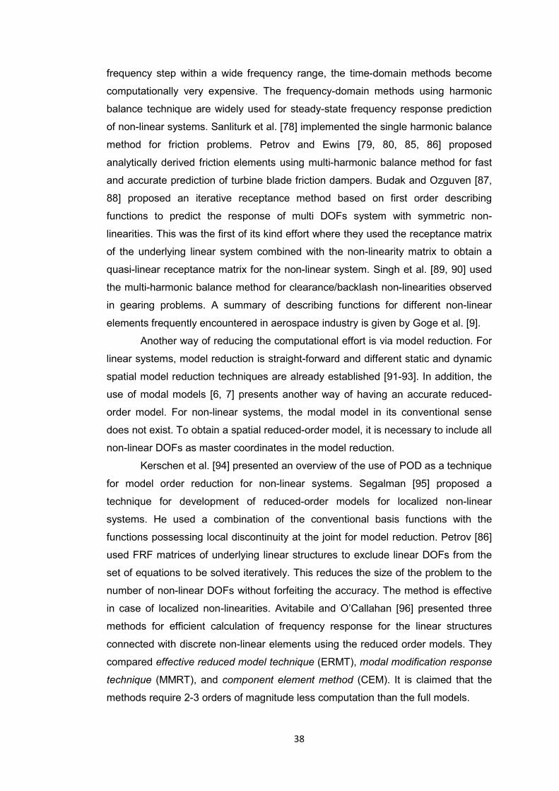
38
frequency step within a wide frequency range, the time-domain methods become
computationally very expensive. The frequency-domain methods using harmonic
balance technique are widely used for steady-state frequency response prediction
of non-linear systems. Sanliturk et al. [78] implemented the single harmonic balance
method for friction problems. Petrov and Ewins [79, 80, 85, 86] proposed
analytically derived friction elements using multi-harmonic balance method for fast
and accurate prediction of turbine blade friction dampers. Budak and Ozguven [87,
88] proposed an iterative receptance method based on first order describing
functions to predict the response of multi DOFs system with symmetric non-
linearities. This was the first of its kind effort where they used the receptance matrix
of the underlying linear system combined with the non-linearity matrix to obtain a
quasi-linear receptance matrix for the non-linear system. Singh et al. [89, 90] used
the multi-harmonic balance method for clearance/backlash non-linearities observed
in gearing problems. A summary of describing functions for different non-linear
elements frequently encountered in aerospace industry is given by Goge et al. [9].
Another way of reducing the computational effort is via model reduction. For
linear systems, model reduction is straight-forward and different static and dynamic
spatial model reduction techniques are already established [91-93]. In addition, the
use of modal models [6, 7] presents another way of having an accurate reduced-
order model. For non-linear systems, the modal model in its conventional sense
does not exist. To obtain a spatial reduced-order model, it is necessary to include all
non-linear DOFs as master coordinates in the model reduction.
Kerschen et al. [94] presented an overview of the use of POD as a technique
for model order reduction for non-linear systems. Segalman [95] proposed a
technique for development of reduced-order models for localized non-linear
systems. He used a combination of the conventional basis functions with the
functions possessing local discontinuity at the joint for model reduction. Petrov [86]
used FRF matrices of underlying linear structures to exclude linear DOFs from the
set of equations to be solved iteratively. This reduces the size of the problem to the
number of non-linear DOFs without forfeiting the accuracy. The method is effective
in case of localized non-linearities. Avitabile and O’Callahan [96] presented three
methods for efficient calculation of frequency response for the linear structures
connected with discrete non-linear elements using the reduced order models. They
compared effective reduced model technique (ERMT), modal modification response
technique (MMRT), and component element method (CEM). It is claimed that the
methods require 2-3 orders of magnitude less computation than the full models.
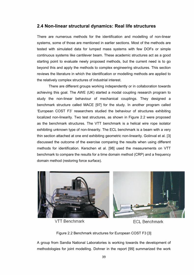
39
2.4 Non-linear structural dynamics: Real life structures
There are numerous methods for the identification and modelling of non-linear
systems, some of those are mentioned in earlier sections. Most of the methods are
tested with simulated data for lumped mass systems with few DOFs or simple
continuous systems like cantilever beam. These academic structures act as a good
starting point to evaluate newly proposed methods, but the current need is to go
beyond this and apply the methods to complex engineering structures. This section
reviews the literature in which the identification or modelling methods are applied to
the relatively complex structures of industrial interest.
There are different groups working independently or in collaboration towards
achieving this goal. The AWE (UK) started a modal coupling research program to
study the non-linear behaviour of mechanical couplings. They designed a
benchmark structure called MACE [97] for the study. In another program called
‘European COST F3’ researchers studied the behaviour of structures exhibiting
localized non-linearity. Two test structures, as shown in Figure 2.2 were proposed
as the benchmark structures. The VTT benchmark is a helical wire rope isolator
exhibiting unknown type of non-linearity. The ECL benchmark is a beam with a very
thin section attached at one end exhibiting geometric non-linearity. Golinval et al. [3]
discussed the outcome of the exercise comparing the results when using different
methods for identification. Kerschen et al. [98] used the measurements on VTT
benchmark to compare the results for a time domain method (CRP) and a frequency
domain method (restoring force surface).
Figure 2.2 Benchmark structures for European COST F3 [3]
A group from Sandia National Laboratories is working towards the development of
methodologies for joint modelling. Dohner in the report [99] summarized the work

40
carried out in this program. They proposed 3 test-beds consisting of different joints
to carry out the benchmark experiments. Segalman et al. [100] reviewed the status
of joint modelling and proposed an integrated roadmap for the future research.
Ferreira [101] during his PhD work built a laboratory structure with 3 beams
to exhibit polynomial stiffness non-linearity. Chong and Imregun [52, 102, 102] used
experimental results obtained using the same structure to test the variable modal
parameter identification method. Elizalde [26] again used the structure to verify the
explicit formulation method for prediction of non-linear response in frequency
domain. The experimental setup used for the exercise is shown in Figure 2.3.
Figure 2.3 Experimental setup used by Ferreira [101] and Elizalde [26]
Platten et al. [53] experimentally verified the non-linear resonant decay method (NL-
RDM) on a fully clamped plate with integral edges exhibiting geometric non-linearity.
Platten et al. [54], in another study, implemented the NL-RDM on a laboratory
structure depicting a ‘wing-store’ model. They excited the first four modes with
increasing level of excitation force to extract the variation of natural frequency and
modal damping. Later each mode is identified separately by plotting the restoring
modal force surface for each mode.
Adams et al. [103, 104] used the restoring force method (RFS) and NIFO
method to characterize the non-linearities and identify the non-linear parameters in
a tire-vehicle suspension system in absence of input measurement. Worden et al.
[105] attempted the identification of non-linearity in an automobile damper using
three different methods available in the literature. They used both time domain
approach (restoring force surface, and neural network) and frequency domain
approach (NIFO method) for identification. Garibaldi et al. [106] successfully used
NIFO method to extract the non-linearities from the experimental data for a scaled
model of a building.
41
Aerospace industry is a challenging sector from non-linear structural
dynamics perspective. There are various attempts to analyze the non-linear aero
structures. Perinpanayagam et al. [107] performed controlled level vibration tests on
an aero-engine casing to detect the non-linear behaviour of the structure. They
extracted the variable modal parameters for the first bending mode of the structure
using SDOF non-linear method. Gloth and Sinapius [108] proposed a method to
extract the amplitude dependency of the modal parameters using sweep sine tests.
The method is implemented on large aircraft structure. Kerschen and Golinval [109]
used a plane-like laboratory structure with non-linear components for the study.
They employed the CRP method in the first stage to extract the underlying linear
model of the structure and the non-linear components. In the second stage, the
underlying linear model obtained from the experiments is used to update the FE
model of the structure. Da Silva and Voroto [110] designed and fabricated a scaled
model of a wing-engine assembly to study the parametrically excited internal
resonance, a phenomenon specific to non-linear structures. Goege [5] proposed a
two-stage methodology to characterize and identify the non-linearity in a ground
vibration test for an aircraft. In the first stage he used different methods to quickly
detect the non-linear modes. In the second stage, he used modal restoring force
surface method to identify the non-linear parameters for each mode. The method is
applied to an actual aircraft in a ground vibration test.
2.5 Summary of the literature review
Non-linear structural dynamics has been of interest to the researchers for more than
four decades. There is an increasing need for accurate prediction methods in order
to reduce the time and the cost involved with the experimentation. This need
coupled with easy availability of computational power acted as a stimulus to the
research in this area.
The ultimate aim of the research in this area is to predict the dynamic
behaviour of a system under different excitation conditions using a computer-based
model of the system. The research progressed in two fundamental branches. The
first branch deals with proposing mathematical models to explain the non-linear
phenomenon. The second branch deals with the identification of the parameters
used in the non-linear models.
The non-linear identification is an inverse problem. It attempts to identify the
system in its mathematical form. The non-linear identification has three steps viz.
non-linearity detection, non-linearity characterization and non-linear parameter
42
extraction. The methods for non-linearity detection are well established and are
widely used in the aerospace and automobile industries. The methods for the
characterization of non-linearity types are still not industrially usable. An experience
based subjective judgement is widely used in the industry for non-linearity
characterization. Extraction of non-linear parameters poses even bigger challenge.
Most of the methods available in the literature are presented for few DOF lumped-
mass systems or simple continuous systems of academic interest. There are some
potential issues when applying these methods to real-life engineering structures.
Recently some attempts have been made to use the identification methods on
complex engineering structures.
Because of the individualistic nature of non-linearities, it is difficult to
propose a universal method for identification to suit all cases. The methods
discussed in the literature have their application region within which they succeed.
Even today, the industry is waiting for a method for non-linear identification which
can be used alongside the main-stream tools like linear modal analysis and FEA
and which is applicable to complex real-life structures.
43
Chapter 3
Non-linearity type identification using a ‘footprint library’ This chapter presents the concept of a ‘footprint library’ to identify the type of non-
linearity in the system. It is observed that the shape of non-linear restoring force
curve is unique to the type of non-linearity. A library of non-linear restoring force
curves, generated using a simple 2-DOF system with different types of non-
linearities is presented. Two methods are proposed for non-linearity type
characterization. In the first method, the footprint library is used as a look-up chart to
identify the type of non-linearity in the system by visual comparison. In the second
method, a shape-matching algorithm is proposed to quantify the match between the
shape of a non-linear restoring force curve obtained for any non-linear structure and
the shape of the curves from the footprint library. The methods are validated on
simulated data for a cantilever beam with different non-linearities.
3.1 Introduction
Non-linearity characterization is an important step in non-linear system
identification. It encompasses the task of locating non-linear DOFs and of finding
the type and the form of non-linearities in the system. After non-linearities are
characterized successfully, the non-linear parameters are identified by posing non-
linear parameter extraction as an optimization problem, which is solved by using the
available methods for optimization. Different methods for non-linearity
characterization are proposed in the literature [9, 20, 22, 29, 30, 111]. Almost all of
these methods are based on some subjective judgement.
Elizalde [26] observed that the variation of non-linear restoring force with
excitation frequency produces a unique ‘footprint’ for each type of non-linearity. This
idea is extended in the current research to present a collection of footprints for
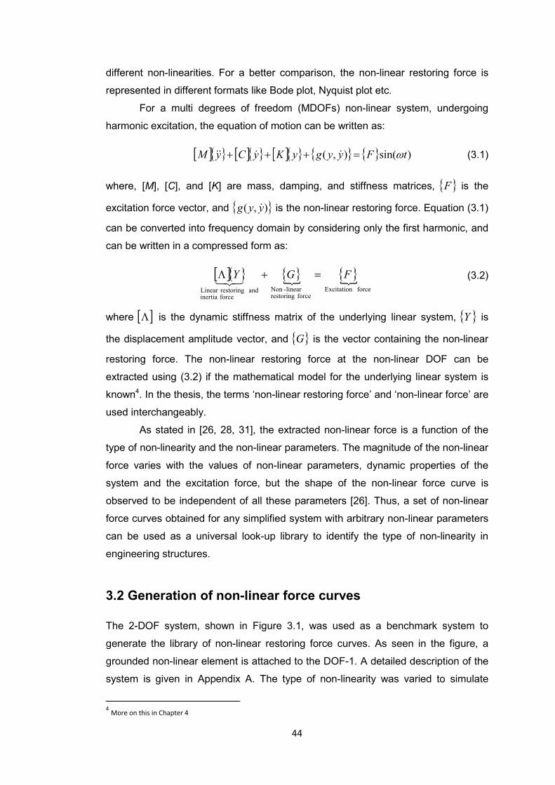
44
different non-linearities. For a better comparison, the non-linear restoring force is
represented in different formats like Bode plot, Nyquist plot etc.
For a multi degrees of freedom (MDOFs) non-linear system, undergoing
harmonic excitation, the equation of motion can be written as:
[ ]{ } [ ]{ } [ ]{ } { } { } )sin(),( tFyygyKyCyM ω=+++ &&&& (3.1)
where, [M], [C], and [K] are mass, damping, and stiffness matrices, { }F is the
excitation force vector, and { }),( yyg & is the non-linear restoring force. Equation (3.1)
can be converted into frequency domain by considering only the first harmonic, and
can be written in a compressed form as:
[ ]{ } { }{ { }{force Excitation
force restoringlinear -Non
force inertiaand restoringLinear
FGY =+Λ 321 (3.2)
where [ ]Λ is the dynamic stiffness matrix of the underlying linear system, { }Y is
the displacement amplitude vector, and { }G is the vector containing the non-linear
restoring force. The non-linear restoring force at the non-linear DOF can be
extracted using (3.2) if the mathematical model for the underlying linear system is
known4. In the thesis, the terms ‘non-linear restoring force’ and ‘non-linear force’ are
used interchangeably.
As stated in [26, 28, 31], the extracted non-linear force is a function of the
type of non-linearity and the non-linear parameters. The magnitude of the non-linear
force varies with the values of non-linear parameters, dynamic properties of the
system and the excitation force, but the shape of the non-linear force curve is
observed to be independent of all these parameters [26]. Thus, a set of non-linear
force curves obtained for any simplified system with arbitrary non-linear parameters
can be used as a universal look-up library to identify the type of non-linearity in
engineering structures.
3.2 Generation of non-linear force curves
The 2-DOF system, shown in Figure 3.1, was used as a benchmark system to
generate the library of non-linear restoring force curves. As seen in the figure, a
grounded non-linear element is attached to the DOF-1. A detailed description of the
system is given in Appendix A. The type of non-linearity was varied to simulate
4 More on this in Chapter 4

several types of n
structures. Different
clearance, friction a
footprint library.
Figure 3
The displacem
harmonic-balance co
method to generat
measurements of a fi
The numerica
range, which is typi
frequency response
experimental measur
curve. For example,
corresponding to sta
frequency step sine
realized. For genera
increasing step sine
stiffness non-linearit
corresponding to the
45
non-linear systems commonly encountere
non-linearities like cubic stiffness (softenin
nd a combination of all these types are c
3.1 The two DOF system used to generate fo
ment response for the system was captured
ode, FORSE [4]. The code uses the single
e displacement responses, which simul
irst-order frequency response on a structure.
ally-predicted response can be multi-valued f
ical of some non-linearities. Figure 3.2 sh
showing both the stable and the unsta
rements, it is only possible to realize the stab
, with an increasing frequency step sine t
able branch 1 is realizable. Alternatively,
test, the response corresponding to stable
ating the footprint library, the response cor
test was used for all non-linearities except t
y. For softening cubic stiffness non-linea
decreasing step-sine test was used.
ed in engineering
ng and hardening),
considered for the
ootprint library
using an in-house
e-harmonic-balance
ates experimental
for some frequency
hows one of such
able branches. In
ble branches of the
test, the response
with a decreasing
e branch 2 can be
rresponding to the
the softening cubic
arity, the response

46
Figure 3.2 A typical frequency response curve for cubic stiffness non-linearity
3.3 Footprints of different non-linearities
A total of ten different types of non-linear forces are included in the footprint library.
The cases considered are as follows:
(1) Cubic stiffness with hardening behaviour
(2) Cubic stiffness with softening behaviour
(3) Clearance
(4) Friction dominated with stick phenomenon
(5) Friction dominated with slip phenomenon
(6) Stick-slip type friction
(7) Combined cubic stiffness and clearance
(8) Combined cubic stiffness and friction
(9) Combined clearance and friction
(10) Combined cubic stiffness, clearance, and friction.
The following section presents the plots of non-linear force for all ten cases. The
non-linear force is plotted in the vicinity of the first resonance of the system. For
each figure, the plot on the left shows the magnitude of non-linear force plotted
against the frequency and the plot on the right is a Nyquist plot. Since only the
shape of the plot is of primary importance, the scale is not shown on the plot axes.

47
3.3.1 Cubic stiffness non-linearity
Figures 3.3 and 3.4 show the non-linear force for the cubic stiffness non-linearity
with hardening and softening behaviour respectively. For hardening type non-
linearity, the non-linear force increases continuously till the resonance frequency,
and then drops suddenly to a lower value. This drop is corresponding to the jump in
the frequency response. In the Nyquist plot, it traces an arc in the forth quadrant.
(a) (b)
Figure 3.3 Non-linear force: Cubic stiffness non-linearity (hardening)
(a) (b)
Figure 3.4 Non-linear force: Cubic stiffness non-linearity (softening)
For the softening cubic stiffness non-linearity, the non-linear force jumps to a higher
value at the resonance frequency, and then gradually reduces to zero as the system
moves away from the resonance. The Nyquist plot traces an arc in the positive Y-
axis region. This observation is justified by the fact that the non-linear force for the
softening cubic stiffness non-linearity is 180 degrees out of phase with the
displacement.
Frequency
Mag
nitu
de o
f non
-line
ar fo
rce
0
0
Re (Non-linear force) Im
ag (N
on-li
near
forc
e)
Frequency
Mag
nitu
de o
f non
-line
ar fo
rce
0
0
Re (Non-linear force)
Imag
(Non
-line
ar fo
rce)

48
3.3.2 Clearance non-linearity
The clearance non-linearity was modelled using a bi-linear stiffness spring with the
clearance gap (yc) and the clearance stiffness (Kz) as the non-linear parameters.
Once the clearance gap is closed, an additional stiffness is coupled to the system.
Figure 3.5 shows the variation of the non-linear force for clearance non-linearity.
(a) (b)
Figure 3.5 Non-linear force: Clearance non-linearity
At first sight, the shape of the plots looks similar to that of the hardening type
cubic stiffness non-linearity. But the close observation of the plots in the region
away from the resonance shows that the non-linear force for clearance non-linearity
is zero until the displacement at the non-linear DOF exceeds the gap distance, and
increases sharply after the gap closure. For the cubic stiffness non-linearity, the
non-linear force shows a steady increment. An enlarged view of the comparison of
the two plots is shown in Figure 3.6.
Figure 3.6 Comparison of cubic stiffness and clearance non-linearity
Frequency
Mag
nitu
de o
f non
-line
ar fo
rce
0
0
Re (non-linear force)
Imag
(non
-line
ar fo
rce)
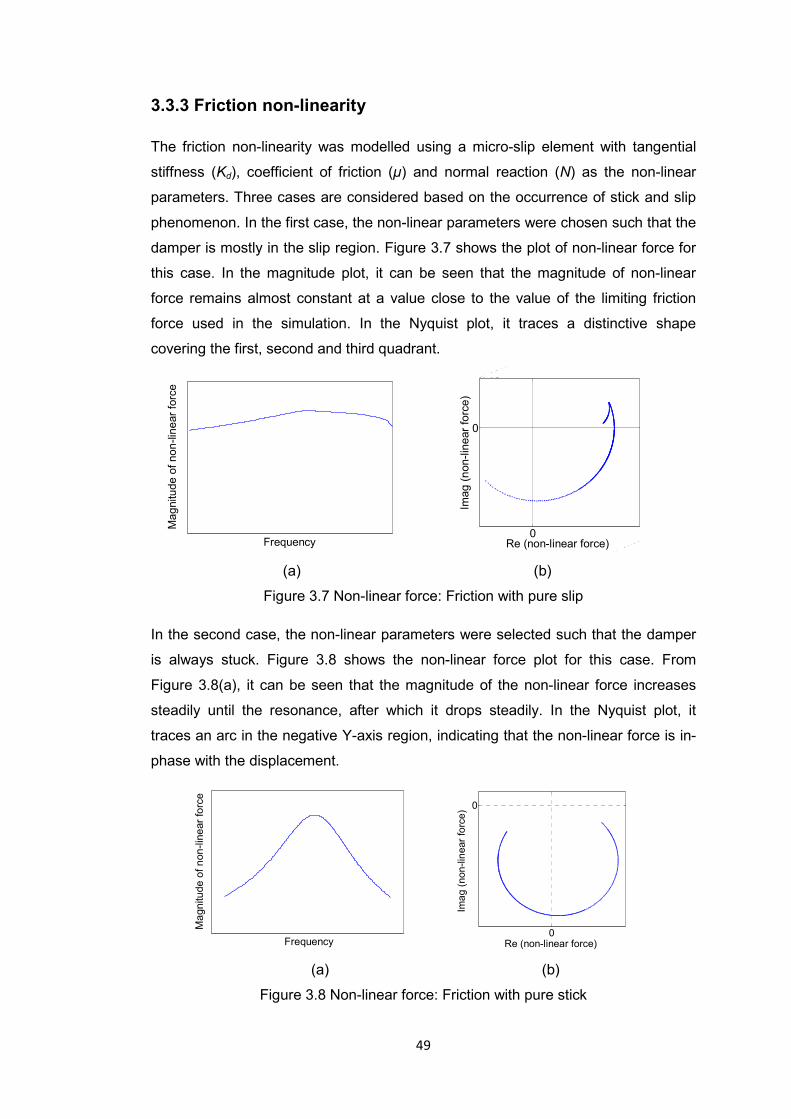
49
3.3.3 Friction non-linearity
The friction non-linearity was modelled using a micro-slip element with tangential
stiffness (Kd), coefficient of friction (µ) and normal reaction (N) as the non-linear
parameters. Three cases are considered based on the occurrence of stick and slip
phenomenon. In the first case, the non-linear parameters were chosen such that the
damper is mostly in the slip region. Figure 3.7 shows the plot of non-linear force for
this case. In the magnitude plot, it can be seen that the magnitude of non-linear
force remains almost constant at a value close to the value of the limiting friction
force used in the simulation. In the Nyquist plot, it traces a distinctive shape
covering the first, second and third quadrant.
(a) (b)
Figure 3.7 Non-linear force: Friction with pure slip
In the second case, the non-linear parameters were selected such that the damper
is always stuck. Figure 3.8 shows the non-linear force plot for this case. From
Figure 3.8(a), it can be seen that the magnitude of the non-linear force increases
steadily until the resonance, after which it drops steadily. In the Nyquist plot, it
traces an arc in the negative Y-axis region, indicating that the non-linear force is in-
phase with the displacement.
(a) (b)
Figure 3.8 Non-linear force: Friction with pure stick
Frequency
Mag
nitu
de o
f non
-line
ar fo
rce
0x 10-3
0
x 10-3
Re (non-linear force)
Imag
(non
-line
ar fo
rce)
Frequency
Mag
nitu
de o
f non
-line
ar fo
rce
0
0
Re (non-linear force)
Imag
(non
-line
ar fo
rce)

50
In the third case, the parameters were chosen such that the damper experiences a
stick-slip condition in the frequency range considered. Figure 3.9 shows the plot for
the non-linear force for this case. From the magnitude plot, the regions of stick and
slip can easily be identified. The non-linear force increases steadily till the damper
starts slipping. In the slip region, the force remains nearly constant. In the Nyquist
plot, two arcs of different radii, corresponding to stick and slip, can be identified.
(a) (b)
Figure 3.9 Non-linear force: Friction with stick and slip
3.3.4 Combination of different non-linearities
In many practical cases, two or more types of non-linearities may co-exist in the
system. If any one type is overpowering the others, then the shape of the non-linear
force curve remains similar to the footprint of the dominant non-linearity type. If two
or more non-linearities are contributing in equal percentage towards the non-linear
force, the resultant non-linear force curve can take a completely different shape. To
identify the type of non-linearity in such cases, the footprint library is extended to
include some combined non-linearity types. While generating the footprints of
combined non-linearities, the non-linear parameters were selected such that each
non-linearity type contributes in equal percentage in the total non-linear restoring
force, when summed over the frequency range.
Figure 3.10 shows the footprint for combined cubic stiffness and clearance
non-linearity. The shape of the footprint is very much similar to the individual
clearance footprint as shown in Figure 3.5.
Frequency
Mag
nitu
de o
f non
-line
ar fo
rce
0
0
Re (non-linear force)
Imag
(non
-line
ar fo
rce)
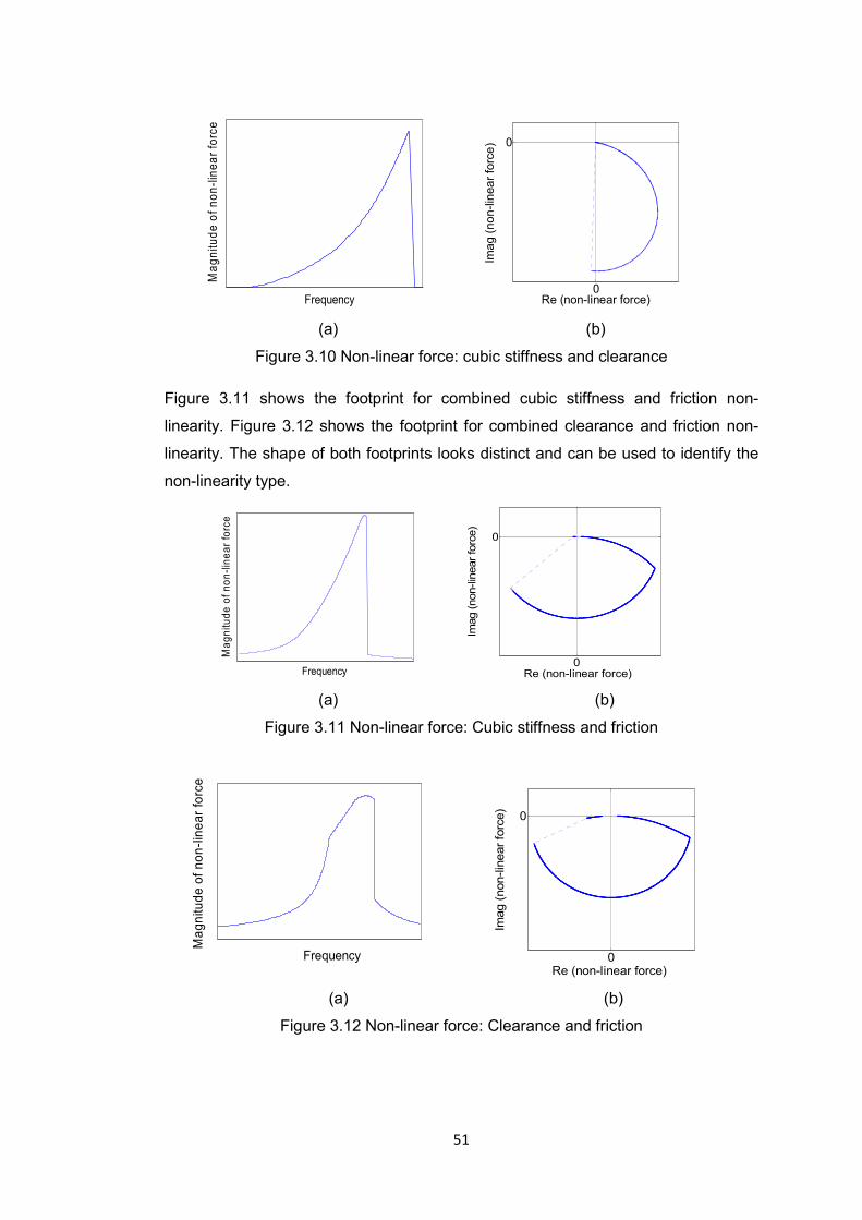
51
(a) (b)
Figure 3.10 Non-linear force: cubic stiffness and clearance
Figure 3.11 shows the footprint for combined cubic stiffness and friction non-
linearity. Figure 3.12 shows the footprint for combined clearance and friction non-
linearity. The shape of both footprints looks distinct and can be used to identify the
non-linearity type.
(a) (b)
Figure 3.11 Non-linear force: Cubic stiffness and friction
(a) (b)
Figure 3.12 Non-linear force: Clearance and friction
Frequency
Mag
nitu
de o
f non
-line
ar fo
rce
0
0
Re (non-linear force)
Imag
(non
-line
ar fo
rce)
Frequency
Mag
nitu
de o
f non
-line
ar fo
rce
0
0
Re (non-linear force)
Imag
(non
-line
ar fo
rce)
Frequency
Mag
nitu
de o
f non
-line
ar fo
rce
0
0
Re (non-linear force)
Imag
(non
-line
ar fo
rce)

52
Figure 3.13 shows the footprint for combined cubic stiffness, clearance, and friction
non-linearity. From the magnitude plot, it is difficult to identify the type of non-
linearity. The Nyquist plot also looks similar to the footprint in Figure 3.11.
(a) (b)
Figure 3.13 Non-linear force: Cubic stiffness, clearance and friction
The footprints of different non-linearities, as presented above, can be collected to
form a library of curves. The library can be used as a look-up chart to qualitatively
comment on the type of non-linearity in the structure. A combined chart with all
types is shown in Figures 3.14 and 3.15.
Frequency
Mag
nitu
de o
f non
-line
ar fo
rce
0
0
Re (non-linear force)
Imag
(non
-line
ar fo
rce)
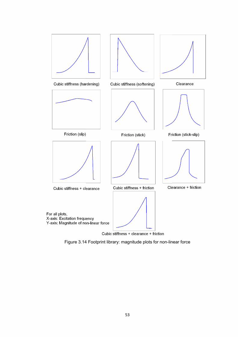
Figure 3.14
53
4 Footprint library: magnitude plots for non-lin
near force

Figure 3.1
The library can be e
commonly occurring
friction are clearly dis
54
15 Footprint library: Nyquist plots for non-line
xtended further to accommodate other type
in engineering structures. It can be seen th
stinguishable whereas the others are more di
ear force
es of non-linearities
hat some types like
fficult to identify.

55
3.4 Quantitative comparison using shape-matching algorithm
The footprint library presented in the section 3.3 uses a subjective judgement to
identify the type of non-linearity. It is observed that some non-linearities are difficult
to distinguish using just the visual comparison. This section presents an objective
way of identifying the type of non-linearity. A shape-matching algorithm is proposed
to measure the closeness of the shape of the extracted non-linear force curve to the
shape of different curves in the footprint library.
The plots in the footprint library presented in the earlier section are not
suitable to use for a quantitative comparison as the frequency axis is difficult to
normalize. For a better quantitative comparison, the non-linear force is plotted
against the magnitude of relative displacement between the non-linear DOFs. As
the plot of the non-linear force is used only to identify the non-linearity type, and not
the strength of the non-linearity or the non-linear parameters at this stage, it is
possible to normalize both axes to unity.
A sample plot showing the non-linear force for cubic stiffness non-linearity is
presented in Figure 3.16. Since the non-linear force is expressed directly as a
function of relative displacement, it completely eliminates the dependence of the
shape of the curve on the system under consideration.
Figure 3.16 Normalized footprint for cubic stiffness
3.4.1 Generation of footprint curves
Since this representation of non-linear force does not depend on the system, the
footprints can be generated using the mathematical expressions for the non-
linearities. The expressions based on the harmonic balance method were used to
generate the footprints. The non-linear force was calculated using the expressions

56
shown in Table 3.1 assuming a grounded non-linearity. The relative displacement
amplitude, (Yi - Yj), at the non-linear DOF was varied from 0 to 1 uniformly. Later,
the non-linear force was normalized to unity to have a library of footprints with
normalized X and Y axes. Similar to the earlier footprints for combined non-
linearities, the parameters were chosen such that each non-linearity contributes
equally towards the non-linear force. The library of footprints is shown in Figure
3.17.
Table 3.1 Expressions for non-linear restoring force [2, 75]
Type of non-linearity
Magnitude of non-linear force
Cubic stiffness 3)(43
jicub YYg −= β
where β is the coefficient of cubic stiffness non-linearity, Yi
and Yj are the amplitudes of displacement at ith and jth DOF
respectively.
Clearance
⎥⎥⎦
⎤
⎢⎢⎣
⎡
−−+−
−= c
ji
ccc
jizcle
YYyYYK
g θθθππ
cos)(
4)2sin(2
2)(*
⎟⎟⎠
⎞⎜⎜⎝
⎛
−= −
)(sin 1
ji
cc YY
yθ
where, Kz is the additional stiffness after the clearance gap is
closed, yc is the gap distance.
Friction Stick region: ( )lll
jidfri YYKg θθθ
πcossin
)(−
−=
Slip region: ⎟⎟⎠
⎞⎜⎜⎝
⎛
−−
−=
)(14
jid
fri
YYKNNg μ
πμ
⎟⎟⎠
⎞⎜⎜⎝
⎛
−−= −
)(21cos 1
jidl YYK
Nμθ
Where, Kd is the tangential stiffness in stick region, N is the
normal reaction, and μ is the coefficient of friction.

Figure 3.17 Lib
3.4.2 Shape-matc
An algorithm is propo
curve extracted for a
library. The ‘match’
linearity in the struct
average distance b
closeness. A numeric
evaluate the Euclidia
curves is significantly
Since the num
non-linear parameter
comparison. Four op
scaling, Y-axis scalin
57
brary of normalized footprints for quantitative
ching algorithm
osed to numerically compare the shape of t
any structure with the shape of different curv
between two curves is examined to identif
ture. If any two curves are normalized on b
etween the two curves can be treated
cal quantity called ‘sum of squared distance
an distance between the two curves. If the
y lower, the curves can be said to have a goo
merical value of the extracted non-linear for
rs in the system, the curves must be norm
erations of linear transformation viz. translati
ng and rotation about Z-axis are performed
e comparison
he non-linear force
ves in the footprint
fy the type of non-
both axes, then the
as a measure of
e’ (SSD) is used to
SSD value for two
od match.
rce is a function of
malized before the
ion to origin, X-axis
d on the extracted

58
non-linear force curve before the comparison. Figure 3.18 depicts the four steps on
a typical non-linear force curve. The blue curve is for clearance non-linearity from
the footprint library and the red curve is the extracted non-linear force curve.
Figure 3.18 Comparison steps for shape-matching
Once the extracted non-linear force curve and the curve from the footprint library
are aligned properly for comparison, the Euclidian distance between the two curves,
represented by the SSD, is calculated as:
( )∑=
−=N
ii
BE YYSSD1
2 (3.3)
where, EY is the Y coordinate of extracted non-linear force curve and BY is the Y
coordinate of the benchmark curve. The curves for which the SSD value is the least
are said to be in a close match, hence identifying the type of non-linearity for the
extracted curve. Figure 3.19 show the flowchart for the shape-matching algorithm.
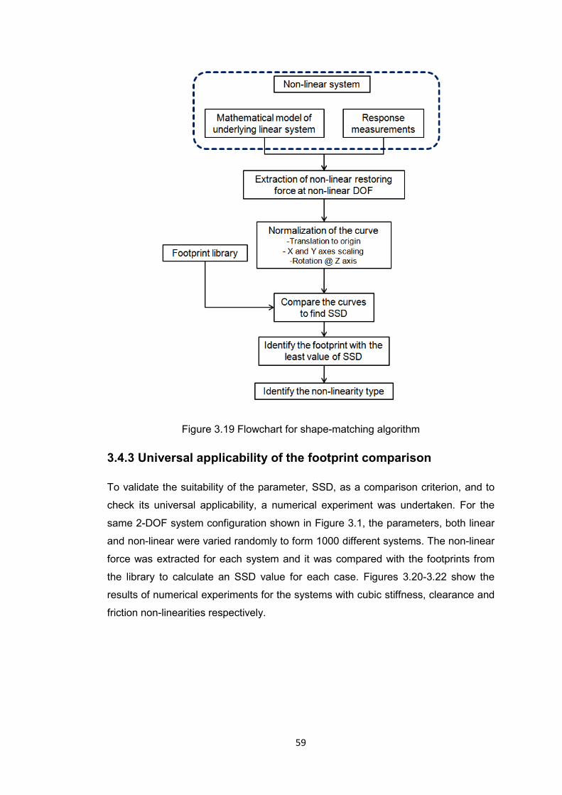
59
Figure 3.19 Flowchart for shape-matching algorithm
3.4.3 Universal applicability of the footprint comparison
To validate the suitability of the parameter, SSD, as a comparison criterion, and to
check its universal applicability, a numerical experiment was undertaken. For the
same 2-DOF system configuration shown in Figure 3.1, the parameters, both linear
and non-linear were varied randomly to form 1000 different systems. The non-linear
force was extracted for each system and it was compared with the footprints from
the library to calculate an SSD value for each case. Figures 3.20-3.22 show the
results of numerical experiments for the systems with cubic stiffness, clearance and
friction non-linearities respectively.

60
Figure 3.20 Numerical experiments: cubic stiffness non-linearity
Figure 3.21 Numerical experiments: clearance non-linearity

61
Figure 3.22 Numerical experiments: friction
It can be seen that for all three cases, when the non-linearity type is
matched correctly, the SSD value is the smallest irrespective of the system
parameters. For cubic stiffness non-linearity, the SSD value is zero throughout the
experiments when compared with the cubic stiffness non-linearity footprint. This
suggests that after the linear transformations, the two curves lie exactly on top of
each other. For other two non-linearities, the SSD value is not zero when compared
with the corresponding footprint, but still it is significantly lower than the other SSD
values so as to identify the correct non-linearity type.
For combined non-linearities, the footprints in the library are generated
based on an assumption of equal contribution by each non-linearity. The
contribution of each non-linearity in the total non-linear force is calculated over the
entire frequency range considered
∑=
=f
s
tot
ii
GGC
ω
ωω ωω
)()( (3.4)
Where, iC is the contribution of ith type of non-linearity, iG is the non-linear force
due to ith non-linearity type, totG is the total non-linear force, sω and fω are the
start and end frequencies in the considered frequency range. In the numerical
experiments, the equal contribution constraint was not incorporated. Thus, the
systems with randomly generated parameters had unequal contribution of different
non-linearities. Figure 3.23 shows the results of numerical experiments for
combined clearance and friction non-linearity.
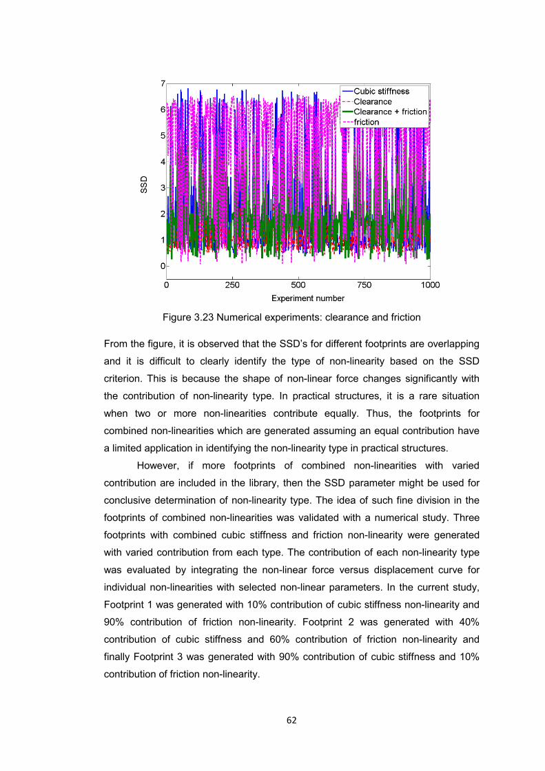
62
Figure 3.23 Numerical experiments: clearance and friction
From the figure, it is observed that the SSD’s for different footprints are overlapping
and it is difficult to clearly identify the type of non-linearity based on the SSD
criterion. This is because the shape of non-linear force changes significantly with
the contribution of non-linearity type. In practical structures, it is a rare situation
when two or more non-linearities contribute equally. Thus, the footprints for
combined non-linearities which are generated assuming an equal contribution have
a limited application in identifying the non-linearity type in practical structures.
However, if more footprints of combined non-linearities with varied
contribution are included in the library, then the SSD parameter might be used for
conclusive determination of non-linearity type. The idea of such fine division in the
footprints of combined non-linearities was validated with a numerical study. Three
footprints with combined cubic stiffness and friction non-linearity were generated
with varied contribution from each type. The contribution of each non-linearity type
was evaluated by integrating the non-linear force versus displacement curve for
individual non-linearities with selected non-linear parameters. In the current study,
Footprint 1 was generated with 10% contribution of cubic stiffness non-linearity and
90% contribution of friction non-linearity. Footprint 2 was generated with 40%
contribution of cubic stiffness and 60% contribution of friction non-linearity and
finally Footprint 3 was generated with 90% contribution of cubic stiffness and 10%
contribution of friction non-linearity.

63
The footprints were compared with a set of non-linear force curves for 2-
DOF system with the combined cubic stiffness and friction non-linearity, and
randomly chosen linear and non-linear parameters. Figure 3.24 shows the results of
the numerical study. Each dot in the figure represents a 2-DOF system. The X axis
shows the contribution of cubic stiffness non-linearity in the system, and the Y axis
shows the SSD value which is normalized to the maximum SSD value obtained in
the set.
Figure 3.24 Comparison with finer footprints for cubic stiffness and friction
It can be observed from the figure that the SSD for all three footprints vary as the
contribution of the cubic stiffness non-linearity in the system changes. The SSD for
a footprint is the smallest when the contribution of non-linearities in the system
matches with the contribution of non-linearities in the footprint. For example, for
Footprint 1, with 10% cubic stiffness non-linearity and 90% friction non-linearity, the
SSD value is the smallest, when the contribution of cubic stiffness non-linearity in
the system is around 10%. Similar trend is observed for the other two cases.
Thus, if the footprint library is expanded to include the footprints of combined
non-linearities with un-equal contribution, then it would be, in principle, possible to
correctly identify the type of non-linearities in the system along with the percentage
contribution of each non-linearity.

64
3.4.4 Numerical examples
The two methods for non-linearity characterization presented in the chapter are
exemplified using numerically synthesized data for Validation structure-1, a
cantilever beam with non-linearity at the free end. The details of the beam are
presented in Appendix B. The study considers three cases with different non-
linearities, and the details of the type of non-linearity and the non-linear parameters
used in the study are presented in Table 3.2.
Table 3.2 Summary of non-linear parameters used for validation
Case Type of non-linearity Non-linear parameters
1 Cubic stiffness β =5e3 Nm-3
2 Friction Kd = 50 N/m; µN = 1e-3 N
3 Cubic stiffness + friction β =5e8 Nm-3 Kd = 10 N/m; µN = 3e-3 N
The synthesized non-linear response data for the beam was generated using the in-
house code FORSE [4]. The non-linear restoring force at the non-linear DOF is
extracted using the spatial method described in Chapter 4 of the thesis5. The
extracted non-linear force for all three cases was used for visual comparison with
the footprint library presented in Section 3.2. For validation of the second method,
the non-linear restoring force for all three cases was numerically compared with
different footprints to evaluate the SSD value for each footprint. The SSD values for
all cases are summarized in Table 3.3.
Figure 3.25 shows a plot of non-linear restoring force at the non-linear DOF
for case 1. The shape of the plot resembles both the cubic stiffness footprint and the
clearance footprint. Figure 3.26 shows the non-linear force for Case 1 overlaid on
top of the footprints of different non-linearities. From the figure, it can be seen that
the extracted non-linear force curve clearly matches with the cubic stiffness non-
linearity footprint. This observation is strengthened by the least SSD value for the
cubic stiffness footprint shown in Table 3.3, identifying the type of non-linearity
correctly.
5 Extracting the non‐linear restoring force for a MDOF system is a challenge in itself. The different methods for extraction of non‐linear restoring force are presented in subsequent chapters of the thesis

65
Figure 3.25 Non-linear force for case 1 (cubic stiffness)
Figure 3.26 Quantitative comparison for Case 1
Figure 3.27 shows the plot of the non-linear force for case 2, with friction
non-linearity. From the visual comparison of the shape of this curve with the
footprints, it is difficult to reach any conclusion. When the non-linear force is
compared with the footprints to find the SSD value, the slip-dominated friction non-

66
linearity is identified as the one with the least SSD value. Figure 3.28 shows the
quantitative comparison with the footprints for Case 2.
Figure 3.27 Non-linear force for Case 2 (friction)
Figure 3.28 Quantitative comparison for Case 2
In Case 3, a combined cubic stiffness and friction non-linearity was used.
For the system with selected non-linear parameters, the cubic stiffness non-linearity
contributes 84% towards the non-linear force. In Figure 3.29, the shape of
magnitude versus frequency plot resembles the cubic stiffness non-linearity footprint

67
but the Nyquist plot shows a different shape. The SSD value for combined cubic
stiffness and clearance non-linearity is found to be the least. The SSD value for the
cubic stiffness non-linearity is the next lowest. Figure 3.30 shows the result of the
shape-matching algorithm for Case 3.
Figure 3.29 Non-linear force for Case 3 (cubic stiffness + friction)
Figure 3.30 Quantitative comparison for Case 3

68
Table 3.3 Summary of the quantitative comparison
Footprint type Sum of squared distance (SSD)
Case 1 Case 2 Case 3
Cubic stiffness 9.8×10⁻⁴ 5.59 0.33 Clearance 1.50 3.41 1.23
Friction (slip) 6.60 2.06 6.36
Friction (stick) 2.09 3.70 1.76
Friction (stick-slip) 6.67 2.15 6.42
Cubic stiffness + clearance 0.45 5.32 0.29 Cubic stiffness + friction 1.26 4.41 0.97
Clearance + friction 2.37 3.41 2.04
Cubic stiffness + clearance + friction 1.13 4.57 0.81
To evaluate the effect of noise on the quantitative method of non-linearity
characterization, data for the same three cases was polluted with 7.5% random
noise. The non-linear force was extracted for noisy measurements, and it was
compared with the footprints from the library. Figure 3.30 shows the comparison of
the extracted non-linear force with the footprint library for Case 3, combined cubic
stiffness and friction non-linearity. Table 3.4 shows presents the detailed results for
all three cases with noise. It can be observed that owing to noisy measurements,
the SSD values are a bit higher than the corresponding values for clean data. Still,
the correct type of non-linearity can be identified for Case 1 and 2.

69
Figure 3.31 Quantitative comparison for Case 3 with 7.5% noise
Table 3.4 Summary of the quantitative comparison with noise
Footprint type Sum of squared distance (SSD)
Case 1 Case 2 Case 3
Cubic stiffness 0.153 6.21 0.84 Clearance 1.62 3.67 1.53
Friction (slip) 5.94 2.31 5.81
Friction (stick) 1.89 3.77 1.75
Friction (stick-slip) 5.99 2.53 5.87
Cubic stiffness + clearance 0.45 5.71 0.87
Cubic stiffness + friction 1.13 4.44 0.94
Clearance + friction 2.12 3.15 1.96
Cubic stiffness + clearance + friction 1.02 4.63 0.96
70
3.5 Concluding remarks
A novel idea of collecting the non-linear restoring force curves for different non-
linearities to form a ‘footprint library’ has been proposed in the chapter. This
footprint library can be used for non-linearity characterization, which forms an
important step in non-linear system identification. The shape of the non-linear
restoring force curves was found to be unique to the type of non-linearity and
independent of the system. The main developments of this chapter can be listed as
follows:
• A library of non-linear force footprints for different non-linearities including the
cubic stiffness, clearance, friction, and combination of all three has been
generated using a 2-DOF benchmark system. The library consists of magnitude
versus frequency plots and Nyquist plots for the non-linearities. The library can
be used as a look-up chart for making a judgement on the type of non-linearity in
the system.
• A shape-matching algorithm has been proposed to quantify the match between
the shape of the extracted non-linear force curve and the footprints. The term
SSD indicating the Euclidian distance between the two curves is used as a
measure of closeness of the shape of the curves.
• The proposed methods have been tested on simulated response data for a
cantilever beam with different non-linearities. The methods worked well for the
individual non-linearities.
• For combined non-linearities, the shape of the non-linear force curve was
observed to be dependent on the contribution of each type of non-linearity. With
the current footprint library, it was found difficult to correctly identify the combined
non-linearity type. An idea of including more footprints in the library with varying
contribution of two or more non-linearities has been suggested as a possible
solution to this problem.
• The quantitative comparison has been tested for measurement data with noise. It
has been observed that the type characterization is accurate even for data with
7.5 percent random noise.

71
Chapter 4
Spatial method for non-linear parameter identification This chapter presents a frequency-domain method for a parametric identification of
non-linear systems. The method uses the finite element (FE) model of the
underlying linear system to extract the non-linear restoring force. The magnitude of
the non-linear restoring force at each DOF is used to find the location of the non-
linearity. A genetic algorithm based optimization method is proposed to extract the
non-linear parameters using the non-linear restoring force at the identified non-
linear DOFs. The method allows successful extraction of non-linear parameter
values even when the type of non-linearity is unknown. The method is illustrated on
simulated data for a cantilever beam with cubic stiffness non-linearity. The
robustness of the method in the presence of measurement noise is checked by
artificially polluting the response data with random noise.
4.1 Introduction
Non-linear system identification is an important stage in structural analysis. Once
the non-linear parameters are known as a function of displacement, velocity etc, the
information can be used to predict the response at different operating conditions [4,
79]. Non-linear system identification consists of three stages, namely the detection
of non-linearity, the type characterization, and the non-linear parameter extraction.
Once the non-linearity is detected and characterized, the parameter extraction can
be posed as an optimization problem. In most of the methods, the success of non-
linear parameter extraction depends on the success of the earlier stages of non-
linearity detection and characterization.
The method proposed in this chapter is based on the reverse explicit
formulation proposed by Elizalde [26, 36]. The basic theme of the method is to
recover the non-linear restoring force for a non-linear system by making use of the

72
FE model of the underlying linear system and the measured responses of the
system. In the current research, a genetic algorithm (GA) based optimization
method is used to identify the non-linear parameters. The use of such a method
allows identifying simultaneously several non-linearities of unknown type. The
method has a potential to identify large non-linear structures, which is the prime
advantage. The theoretical formulation of the method is presented in the next
section.
4.2 Theoretical formulation
For a multi DOF system, undergoing harmonic excitation, the equations of motion
can be written as:
[ ]{ } [ ]{ } [ ]{ } { } { } )sin()( tFygyKyCyM ω=+++ &&& (4.1)
where, [ ]M , [ ]C ,and [ ]K are mass, viscous damping, and stiffness matrices, { }F is
the amplitude of excitation force, and { }( )g y is the non-linear restoring force as a
function of displacement.
The solution to (4.1) is multi-harmonic, with significant contributions from
higher order harmonics as shown in [79]. With single-harmonic limitation, assuming
that the response to a harmonic force is also harmonic at the same frequency, and
neglecting the higher order harmonics in the response, (4.1) can be converted into
frequency domain:
[ ] [ ] [ ]( ){ } { } { }FYGYKCiM =+++− ),(2 ωωω (4.2)
where, ( , )G Y ω is the non-linear restoring force as a function of the non-linear
response and excitation frequency. The non-linear restoring force vector can be
written as:
{ } { } [ ]{ }YZFYG −=),( ω (4.3)
where, the linear dynamic stiffness matrix, [ ]Z , can be expressed as:
[ ] [ ] [ ] [ ]( )KCiMZ ++−= ωω 2 (4.4)
If the measured and un-measured DOFs are indicated by subscripts m and u
respectively, (4.3) can be expanded as follows:

73
⎭⎬⎫
⎩⎨⎧⎥⎦
⎤⎢⎣
⎡−
⎭⎬⎫
⎩⎨⎧
=⎭⎬⎫
⎩⎨⎧
u
m
uuum
mumm
u
m
u
m
YY
ZZZZ
FF
GG
(4.5)
If it is assumed that the non-linearity is confined to the measured zone, vector uG
becomes zero, and the un-measured responses can be expressed in terms of
known quantities as:
{ } [ ] { } [ ]{ }( )mumuuuu YZFZY −= −1 (4.6)
Substituting { }uY in (4.5), { }mG can be expressed in terms of the measured
responses as:
{ } { } [ ] [ ] { } [ ]{ }( )( ) [ ]{ }mmmmumuuumumm YZYZFZZFG −−−= −1 (4.7)
The non-linear restoring force vector of (4.7) can be extracted if the excitation force
vector and the underlying FE model are known, and if the non-linearities are
confined to the measured DOFs. This can be a serious limitation when applied to
practical structures, where the measurement at non-linear DOF cannot be
guaranteed. An approximated technique to overcome this limitation is presented in
Section 4.2.5.
4.2.1 Non-linearity detection and characterization
The non-linear force vector for the measured DOFs is used for the detection and
characterization of non-linearity. Assuming that all non-linearities are confined to the
measured zone, a non-zero value in the non-linear restoring force vector detects the
presence and location of non-linearity. The magnitude of the non-linear force at all
measured DOFs is summed over the measured frequency range to get the
accumulated force vector, { }cmG
{ } { }( )∑=
=j
i
GABSG cm
ω
ωω
ω)( (4.8)
This vector is plotted for all measured DOFs to identify the location of non-linearity.
A similar approach to locate the non-linear DOFs is presented in [26, 28].
Once the non-linear DOFs are identified, the shape of the non-linear
restoring force at the non-linear DOFs can be compared with the footprint library
presented in Chapter 3 to characterize the type of non-linearity.
4.2.2 Formulation of the optimization problem

74
Once the non-linear force at the non-linear DOFs is extracted, the non-linear
parameters can be estimated by solving the optimization problem. This section
presents the formulation of the optimization problem.
The non-linear force at the ith DOF, and at a particular excitation frequency,
can be written as a function of np non-linear parameters which are to be identified.
),.........,,,,(4444 84444 76 pn
dczi NKyKfG μβ= (4.9)
The above equation though formulated for cubic stiffness, clearance, and friction
non-linearities at present, can be generalized to incorporate other types as well. The
vibration measurements usually provide response amplitude values at a discrete set
of frequency values. Let nf be the number of frequency lines in the measurement
range. As the non-linear parameters are assumed independent of frequency, one
equation can be written per frequency line. Thus, there are a total of nf equations
with np unknowns. Generally, nf >> np, thus a highly over determined system of
equations is usually available.
In principle, all of the nf equations can be solved by minimizing say the 2-
norm of the error vector, but the response away from the resonance is generally
small, the signal to noise ratio is generally low, and accuracy of modelling is less
important for those frequencies. Thus, the data far away from the resonance can be
ignored in most of the cases.
Thus ns points out of total nf available, can be chosen in the range where the
non-linear force has significant magnitude. The number of points, ns, should be
higher than the number of unknown variables, np, and usually surpasses it
significantly.
The identification problem can be posed as an optimization problem by
formulating the residual at the ith DOF, as:
iifriclecub
i GgggR −++= )( (4.10)
where, Gi is the non-linear force at the ith DOF obtained from (4.7), and cubg , cleg ,
and frig are the expressions based on the harmonic balance method for cubic
stiffness, clearance and friction non-linearities, presented earlier in Table 3.1. This is
a more general formulation considering the presence of different non-linearities at a
particular DOF. This formulation potentially eliminates the need of accurate type
characterization before this step.
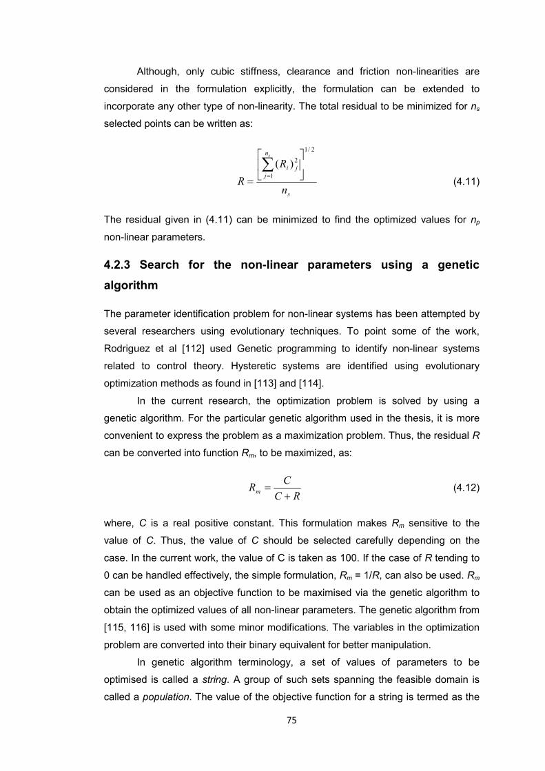
75
Although, only cubic stiffness, clearance and friction non-linearities are
considered in the formulation explicitly, the formulation can be extended to
incorporate any other type of non-linearity. The total residual to be minimized for ns
selected points can be written as:
s
n
jji
n
RR
s2/1
1
2)( ⎥⎦
⎤⎢⎣
⎡
=∑=
(4.11)
The residual given in (4.11) can be minimized to find the optimized values for np
non-linear parameters.
4.2.3 Search for the non-linear parameters using a genetic algorithm
The parameter identification problem for non-linear systems has been attempted by
several researchers using evolutionary techniques. To point some of the work,
Rodriguez et al [112] used Genetic programming to identify non-linear systems
related to control theory. Hysteretic systems are identified using evolutionary
optimization methods as found in [113] and [114].
In the current research, the optimization problem is solved by using a
genetic algorithm. For the particular genetic algorithm used in the thesis, it is more
convenient to express the problem as a maximization problem. Thus, the residual R
can be converted into function Rm, to be maximized, as:
RCCRm +
= (4.12)
where, C is a real positive constant. This formulation makes Rm sensitive to the
value of C. Thus, the value of C should be selected carefully depending on the
case. In the current work, the value of C is taken as 100. If the case of R tending to
0 can be handled effectively, the simple formulation, Rm = 1/R, can also be used. Rm
can be used as an objective function to be maximised via the genetic algorithm to
obtain the optimized values of all non-linear parameters. The genetic algorithm from
[115, 116] is used with some minor modifications. The variables in the optimization
problem are converted into their binary equivalent for better manipulation.
In genetic algorithm terminology, a set of values of parameters to be
optimised is called a string. A group of such sets spanning the feasible domain is
called a population. The value of the objective function for a string is termed as the

76
fitness of the string. In the current formulation, the maximum fitness can reach unity.
It can also be expressed as percentage value. The string with the highest objective
function is called the fittest string. The three basic operators, namely: reproduction,
cross-over, and mutation are used sequentially on the population. The reproduction
operator aims at improving overall fitness of the population. The cross-over operator
ensures a global search, whereas the mutation operator does a fine local search.
These three operators constitute a generation. After the implementation of these
three operators, an improved population emerges. The fitness of population and the
number of generations are used as convergence criteria. In the current algorithm,
the value of Rm tends to unity as the solution converges.
Initially, the upper and lower limits of all non-linear parameters are chosen
based on the engineering judgement. After a predefined number of generations,
called a civilization, the range of the non-linear parameters is refined by analysing
the values taken by the fittest string in the population. With the new range and
increased accuracy for these variables, another civilization is completed. This
process is continued until the convergence criteria are satisfied. Figure 4.1 shows
the flowchart showing one civilization of the GA used.

77
Figure 4.1 Flowchart of the genetic algorithm optimization
Since all possible non-linearities can be included in the formation 6 , the global
optimum solution would correspond to the accurate parameters of the non-linearities
which are actually present in the system. For example, when only one type of non-
linearity is present in the system, the converged solution will yield accurate
parameter values for the correct type of non-linearity, and zero values for
parameters corresponding to the other non-linearities. The genetic algorithm
performs better at finding the global optimum, thus it is suitable for cases when the
type of non-linearity is not known a priori.
4.2.4 Use of binary multipliers to improve the efficiency
When the type of non-linearity is known with certainty, or can be guessed with an
associated probability, the method can be improved by taking into account this 6 In this case, cubic stiffness, clearance and friction non-linearities are considered in the formation

78
information. This is achieved by introducing binary multipliers. In this approach,
weighted residuals are formed for each non-linear force contribution. The residual
non-linear force is written by modifying (4.10) as:
iifriclecub
i GgagagaR −++= )( 321 (4.13)
where all possible non-linear forces, cubg , cleg and frig are multiplied by weighing
constants a1, a2, and a3. If the type of non-linearity is successfully identified prior to
this stage, then the constant corresponding to the identified type takes the value 1
and the other constants take the value 0 for the complete optimization.
If the type of non-linearity can be guessed with an associated probability,
then during each generation of genetic algorithm, these constants take a value
either 0 or 1, which is selected probabilistically. The probability of such value
selection is provided by the user. If the probability of, say clearance non-linearity
(gcle) is the highest, then a2 takes the value 1 more often than a1 and a3. Such a
technique creates more instances in the population which are solved for the most
probable non-linearity; ensuring a faster convergence. The rest of the procedure
remains same with (4.12) giving the total residual to be maximised.
4.2.5 Non-linear parameter identification without full measurement set at non-linear DOFs
Most of the non-linear identification methods in the literature, including the methods
proposed in [26, 37, 38], require the measurement at all non-linear DOFs. It is
sometimes difficult to measure at all non-linear DOFs due to their inaccessible
locations. A slight modification in the equations presented in Section 4.2, along with
the use of spatial reduction methods, enables the extraction of the non-linear
restoring force at the non-linear DOFs when measurements are not taken at these
DOFs.
If it is ensured that the non-linear DOFs are restricted to the un-measured
zone, the vector { }mG becomes zero, and using (4.5), the un-measured response
vector can be represented in terms of known quantities as:
{ } [ ] { } [ ]{ }( )mmmmmuu YZFZY −= + (4.14)
Equation (4.14) involves the inversion of a rectangular matrix, which puts the
mathematical condition of m ≥ u, to be satisfied. Generally, the number of un-
measured DOFs is much higher than the number of measured DOFs (u >> m).

79
Thus, the condition required for the solution of (4.14) is seldom satisfied in practical
cases.
The condition can be satisfied artificially, by reducing the system to Nr DOFs,
such that m ≥ Nr/2, while retaining all non-linear DOFs during the reduction. In the
current research, the improved reduced system (IRS) method of [93] is used for the
system reduction. This method is an extension of the Guyan reduction technique
[91], with inclusion of an extra term to incorporate the inertial effects. The use of
static reduction method results in system matrices which are independent of the
frequency, thus saving a huge computational effort.
Once the reduced model for the system is achieved, (4.14) can be solved by
calculating the pseudo inverse of [ ]muZ . The non-linear force vector, uG , can be
extracted by substituting (4.14) in (4.7):
{ } [ ]{ } [ ] [ ] { } [ ]{ }( )( )( )mmmmmuuumumu YZFZZYZG −+−= + (4.15)
Equation (4.15) gives the non-linear restoring force vector containing non-linear
DOFs. The above technique can be used to extract the non-linear force at the non-
linear DOFs when the location of the non-linearity is known, but no measurements
could be taken at those locations.
The non-linear restoring force at the non-linear DOFs can be used to extract
the non-linear parameters as explained in Sections 4.2.2 and 4.2.3.
4.3 Numerical examples
The proposed method was tested on ‘Validation structure-1’, a cantilever beam with
cubic stiffness non-linearity at the free end. The details of the structure are shown in
Appendix B. Numerically-synthesized data were used to validate the proposed
method. A cubic stiffness non-linearity with non-linear coefficient, β = 5×10⁶ Nm-3
was used for the validation. The response was predicted using the in-house code
FORSE [4]. Figure 4.2 shows the comparison of linear and non-linear responses of
the beam at the non-linear DOF. It is observed that the response is multi-valued in
the frequency range of 32-55 rad/sec. The truncated response, corresponding to
stable branch 1, as explained in Chapter 3 was used for the identification.
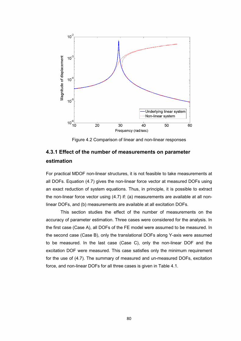
80
Figure 4.2 Comparison of linear and non-linear responses
4.3.1 Effect of the number of measurements on parameter estimation
For practical MDOF non-linear structures, it is not feasible to take measurements at
all DOFs. Equation (4.7) gives the non-linear force vector at measured DOFs using
an exact reduction of system equations. Thus, in principle, it is possible to extract
the non-linear force vector using (4.7) if: (a) measurements are available at all non-
linear DOFs, and (b) measurements are available at all excitation DOFs.
This section studies the effect of the number of measurements on the
accuracy of parameter estimation. Three cases were considered for the analysis. In
the first case (Case A), all DOFs of the FE model were assumed to be measured. In
the second case (Case B), only the translational DOFs along Y-axis were assumed
to be measured. In the last case (Case C), only the non-linear DOF and the
excitation DOF were measured. This case satisfies only the minimum requirement
for the use of (4.7). The summary of measured and un-measured DOFs, excitation
force, and non-linear DOFs for all three cases is given in Table 4.1.

81
Table 4.1 Description of measured DOFs
Case Measured DOFs Un-measured DOFs Excitation
DOF Non-linear
DOF
A {1, 2, 3, ....,20} Nil
19 19 B {1, 3, 5, 7,....,19} {2, 4, 6, 8, …., 20}
C {19} {1, 2, 3, 4,…,18 and 20}
For all three cases, the non-linear force was extracted at all measured DOFs using
(4.7). The accumulated non-linear force for the measured DOFs was used to
identify the location of non-linearity. Figure 4.3 shows the plot of the accumulated
non-linear force at measured DOFs for Case A. It can be seen that the accumulated
non-linear force at DOF#19 is maximum. The non-linear force at other DOFs is
close to zero. Thus, the location of non-linearity at DOF#19 is correctly identified.
Figure 4.3 Identification of non-linearity location (Case A)
The non-linear force at the identified non-linear DOF, plotted against the frequency
and as a Nyquist plot, was used for non-linearity characterization. Figure 4.4 shows
the plot of non-linear force at DOF#19 for Case A. If the shape of the non-linear
force is visually compared with the footprint library presented in Chapter 3, the cubic
stiffness non-linearity can be deduced. This was confirmed when the non-linear
force was numerically compared with the footprints to find the values of SSDs for
different non-linearities. The SSD, when compared with cubic stiffness non-linearity,
was found to have the least value (SSD=0.001), thus identifying the type of non-
linearity.
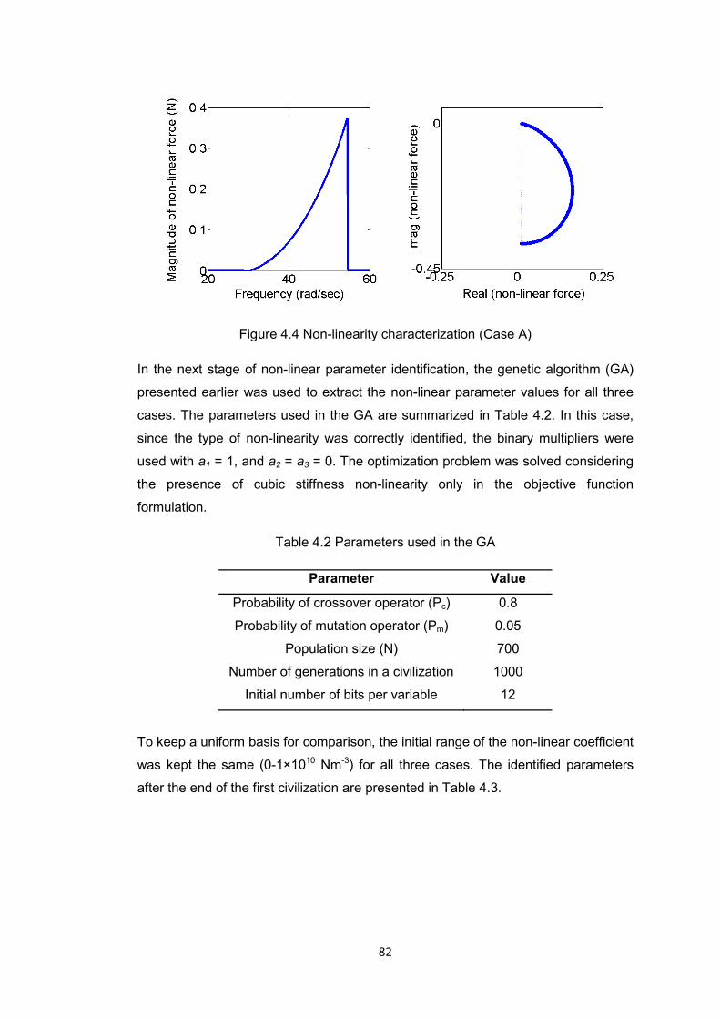
82
Figure 4.4 Non-linearity characterization (Case A)
In the next stage of non-linear parameter identification, the genetic algorithm (GA)
presented earlier was used to extract the non-linear parameter values for all three
cases. The parameters used in the GA are summarized in Table 4.2. In this case,
since the type of non-linearity was correctly identified, the binary multipliers were
used with a1 = 1, and a2 = a3 = 0. The optimization problem was solved considering
the presence of cubic stiffness non-linearity only in the objective function
formulation.
Table 4.2 Parameters used in the GA
Parameter Value
Probability of crossover operator (Pc) 0.8
Probability of mutation operator (Pm) 0.05
Population size (N) 700
Number of generations in a civilization 1000
Initial number of bits per variable 12
To keep a uniform basis for comparison, the initial range of the non-linear coefficient
was kept the same (0-1×10¹⁰ Nm-3) for all three cases. The identified parameters
after the end of the first civilization are presented in Table 4.3.
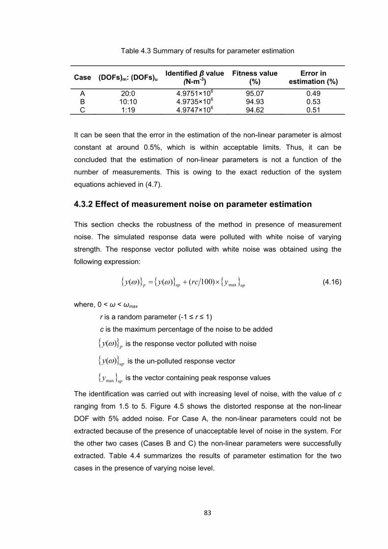
83
Table 4.3 Summary of results for parameter estimation
Case (DOFs)m: (DOFs)u Identified β value
(N-m-3) Fitness value
(%) Error in
estimation (%) A 20:0 4.9751×10⁶ 95.07 0.49 B 10:10 4.9735×10⁶ 94.93 0.53 C 1:19 4.9747×10⁶ 94.62 0.51
It can be seen that the error in the estimation of the non-linear parameter is almost
constant at around 0.5%, which is within acceptable limits. Thus, it can be
concluded that the estimation of non-linear parameters is not a function of the
number of measurements. This is owing to the exact reduction of the system
equations achieved in (4.7).
4.3.2 Effect of measurement noise on parameter estimation
This section checks the robustness of the method in presence of measurement
noise. The simulated response data were polluted with white noise of varying
strength. The response vector polluted with white noise was obtained using the
following expression:
{ } { } { }upupp yrcyy max)100()()( ×+= ωω (4.16)
where, 0 < ω < ωmax
r is a random parameter (-1 ≤ r ≤ 1)
c is the maximum percentage of the noise to be added
{ }py )(ω is the response vector polluted with noise
{ }upy )(ω is the un-polluted response vector
{ }upymax is the vector containing peak response values
The identification was carried out with increasing level of noise, with the value of c
ranging from 1.5 to 5. Figure 4.5 shows the distorted response at the non-linear
DOF with 5% added noise. For Case A, the non-linear parameters could not be
extracted because of the presence of unacceptable level of noise in the system. For
the other two cases (Cases B and C) the non-linear parameters were successfully
extracted. Table 4.4 summarizes the results of parameter estimation for the two
cases in the presence of varying noise level.

84
Figure 4.5 Displacement response with 5% random noise
Table 4.4 Results of parameter estimation in presence of noise
Case Noise level
Identified β value (N-m-3)
Error in estimation (%)
Fitness value (%)
B
c = 1.5 5.353×10⁶ 7.1 18.2
c = 3 5.823×10⁶ 16.5 9.5
c = 5 3.569×10⁶ 28.6 6.1
C
c = 1.5 4.888×10⁶ 2.2 92.7
c = 3 4.805×10⁶ 3.9 91.1
c = 5 4.725×10⁶ 5.5 85.9
It is seen for both cases that the error in parameter estimation increases with the
increase in the noise level. The maximum error in parameter estimation is around
29% for Case B with 5% random noise. It is an interesting observation that the error
is consistently higher in Case B, the case in which a higher number of
measurements was available. This might look counter intuitive, but it is related to
the fact that a highly over-deterministic system of equations is being solved in the
optimization process, and each additional measurement is contributing towards
additional noise in the system.
For Case B, with 1.5% noise, the accuracy of parameter estimation is better;
but the fitness value of the fittest string obtained by the GA is quite low at 18.2%.
This suggests that that there is a scatter in data points of the extracted non-linear

85
force. Figure 4.6 shows the comparison of the extracted and the regenerated non-
linear force curve for this case.
Figure 4.6 Comparison of the extracted and regenerated non-linear force
From the study of the effect of measurement noise on the parameter estimation, it is
observed that the method is robust in the presence of measurement noise for Case
B and Case C. The effect of noise becomes severe as the number of
measurements in the analysis increases.
4.3.3 Effect of binary multipliers on computational efficiency
Binary multipliers are proposed to enhance the computational efficiency of the GA
when the type of non-linearity can be guessed with some associative probability.
This section studies the effect the use of binary multipliers in the GA.
A new set of three cases was considered for the study. In the first case, the
binary multipliers were not used. In the second case, the binary multipliers were
used with a high value of probability assigned to the correct type of non-linearity and
a relatively low value of probability is assigned to the other types. In the third case,
the binary multipliers were used with an equal value of probability assigned to all
non-linearity types. This case corresponds to a situation when the type
characterization fails, and the non-linearity type is not known in advance. The
results for the three cases are compared with the benchmark case where only cubic
stiffness non-linearity is included in the formulation of optimization problem.
The simulated data for the beam without any addition of noise was used for
the analysis. The GA code was terminated after 5000 generations and the results
were recorded. Table 4.5 summarizes the results for the exercise. In the table, Pcub,

86
Pcle, and Pfri denote the probability of the presence of cubic stiffness, clearance and
friction non-linearity. The values correlate to the probabilities with which the binary
multipliers, a1, a2, and a3 take the value of 1 in the simulation. Gcon denotes the
number of generations at which the fittest string was found. It is observed that the
error in parameter estimation is the least when the binary multipliers are used with a
high probability assigned to the correct non-linearity type. The error in the other two
cases is comparable, but the use of the binary multipliers is found to speed-up the
convergence.
Table 4.5 Performance of binary multipliers
Case (Pcub, Pcle, Pfri) Identified β
value (N-m-3)Error (%)
Gcon
Benchmark - 4.9812×10⁶ 0.38 45
1 (1,1,1) 4.8818×10⁶ 2.36 2932
2 (0.9,0.2,0.2) 4.9781×10⁶ 0.44 96
3 (0.5,0.5,0.5) 4.8930×10⁶ 2.14 293
Figure 4.7 shows the plot of the fitness of the fittest string in the population at each
generation for the first 500 generations. It is seen that in the absence of binary
multipliers, the fitness of the fittest string in the population is lower than the fitness
when the binary multipliers are used. The fluctuation in the fitness value is also
more when the binary multipliers are not used.
Figure 4.7 Performance of binary multipliers: fittest string fitness

87
Figure 4.8 shows the plot of the average fitness of the population for each
generation. It is observed that the average fitness is consistently higher in the case
when the binary multipliers are used with the correct type of non-linearity. The
average fitness of the population is the least when binary multipliers are used with
equal probability.
Figure 4.8 Performance of binary multipliers: Average fitness
4.3.4 Effect of the error in the FE model on parameter estimation
It is very difficult to obtain an accurate finite element model for practical structures,
even in case of a linear structure. After correlating the model with the experimental
data and updating it, the error in the FE model may be reduced. For a complex
mechanical structure like the MACE structure, an error of around 5-7% in the natural
frequencies of the first few modes is considered acceptable after the model
updating [63]. The damping values inputted into the FE model are extracted using
modal testing. This is another source of error in the underlying FE model. It is
necessary to evaluate the sensitivity of the estimated non-linear parameters to the
errors in the underlying FE model. This section studies the effect of the errors in the
underlying FE model on the parameter estimation.
The physical properties of the beam were altered by a small amount so that
the change is reflected in the natural frequencies of the beam. The damping ratio for
the first mode was altered to evaluate the effect of the error in damping estimation.
The non-linear identification was carried out with the erroneous FE model of the
beam to extract the non-linear parameters. Table 4.6 shows a summary of the
results. As the identification was carried out with the data covering only the first

88
mode of the beam, the deviation in the first natural frequency of the beam is
recorded in the table. In the table, ωn1 denotes the first natural frequency and η1
denotes the damping ratio for the first mode.
Table 4.6 Effects of the erroneous FE model
Error in the physical properties of the FE model
Error in the damping estimate
Deviation in ωn1
(%)
Identified β
(Nm-3)
Error
(%)
Error in η1 estimation
(%)
Identified
β (Nm-3)
Error
(%)
-5 4.41×10⁶ 11.8 -10 4.98 0.4
-7 4.19×10⁶ 16.2 20 4.98 0.4
-10 3.87×10⁶ 22.6 50 5.07 1.4
It is seen that the effect of the error in damping estimation is negligible. Even with
50% error in the estimation of the damping ratio for the first mode, the error in the
identified non-linear parameter is less than 2%. The effect of the deviation in natural
frequencies on parameter estimation is seen to be significant. Figure 4.9 shows the
plot of the accumulated non-linear force for all DOFs. It is observed that, with an
increase in the error in the underlying FE model, the non-linear force contribution at
the linear DOFs is increasing.
Figure 4.9 Accumulated non-linear force plot
For an erroneous FE model with 5-7% deviation in the first natural frequency value,
which may be acceptable in some cases, the error in parameter estimation is more
than 15%. Thus, it is necessary to obtain an accurate FE model of the structure
before proceeding to the stage of non-linear parameter estimation.

89
4.3.5 Non-linear parameter identification in absence of measurements at non-linear DOFs
This section presents a numerical validation of the technique presented in Section
4.2.5 for non-linear identification in absence of the measurement at the non-linear
DOFs. The details of the measured and un-measured DOFs are given in Table 4.7.
Table 4.7 Case description for non-linear parameter identification in absence of the
measurement at non-linear DOFs
Measured region: (DOFs)m {3, 7, 9, 11, 13, 17}
Un-measured region: (DOFs)u {1, 5, 15, 19, and 2, 4, 6, ..18, 20}
Excitation DOF {19}
Non-linear DOF {19}
From the table, it is observed that the non-linear DOF, DOF#19, is in the un-
measured region. The number of measured DOFs is, m = 6, and the number of un-
measured DOFs is, u = 14. Since the number of measured DOFs is less than the
number of un-measured DOFs, system reduction needs to be performed to satisfy
the constraint, m ≥ u.
The IRS technique was applied to perform a static reduction of system
matrices removing all rotation DOFs. The non-linear DOFs, along with the other
translational DOFs were retained during the reduction. For the reduced system, Nr =
10, and the condition, m ≥ Nr/2 is satisfied. The non-linear force was extracted at the
un-measured DOFs. Figure 4.10 shows a plot of non-linear force against frequency
and the accumulated non-linear force at the un-measured DOFs.
Figure 4.10 Non-linear force at un-measured DOFs
From the plot, it is observed that the non-linear force at the non-linear DOF is
significantly higher in magnitude than that at the other DOFs. The non-linear force at

90
the non-linear DOF is used to extract the non-linear coefficient, β. The value of β is
identified with less than 1% error (β = 4.96×10⁶ N-m-3). Thus, the technique
explained in Section 4.2.5 for the identification of non-linear parameters in the
absence of the measurement at the non-linear DOF works well if the non-linearity
location is correctly identified and retained as master coordinate during the process
of model reduction.
4.4 Concluding remarks
A method for non-linearity detection and non-linear parameter identification has
been proposed in the chapter. The method uses the FE model of the underlying
linear system to extract the non-linear restoring force at non-linear DOFs. A genetic
algorithm based optimization procedure is used to extract the non-linear
parameters. The concept of binary multipliers is introduced to enhance the
computational efficiency of the method. The method is validated on numerically
simulated data for a cantilever beam. The proposed method has the potential to be
used for practical engineering structures with localized non-linearities. The main
developments of the chapter can be listed as follows:
• The proposed method recovers the non-linear restoring force. The accumulated
value of the non-linear force at each DOF is used to locate the non-linearity. It
has been seen that the magnitude of the non-linear force at the non-linear DOF
is significantly higher than that at the linear DOFs.
• The variation of the non-linear force can be used to identify the type of non-
linearity. It has been found that even if the non-linearity type is not known, the
genetic algorithm based optimization accurately extracts the parameter
corresponding to the correct non-linearity type.
• The concept of binary multipliers has been found to be effective in increasing
the computational efficiency of the method if the type of non-linearity can be
guessed with an associative probability.
• The performance of the method has been found satisfactory in the presence of
measurement noise. It has been observed that, in the presence of noise, the
parameter estimation is more accurate when fewer measurements are used.
• The effect of errors in the FE model on parameter estimation is studied. It has
been seen that errors in the mass and stiffness matrices of the FE model has a
significant effect on the accuracy of parameter estimation.

91
• A technique, which uses model reduction, is proposed to identify the non-linear
parameters when the response at non-linear DOFs is not measured. The
technique works accurately on the system when non-linear DOFs are retained
during the model reduction.
92
Chapter 5
Non-linear identification using modal models and response models This chapter presents two methods for non-linear parameter identification, with the
distinctive feature that the methods do not use the FE model of the underlying linear
system. The first method, called improved hybrid modal technique (I-HMT), uses a
hybrid spatial-modal formulation. The non-linearities are described in spatial
coordinates whereas the underlying linear system is represented using a modal
model. The non-linear modal vector (NMV), containing the information about the
non-linear restoring force, is extracted for the modes in the measured frequency
range. Later, the NMV is used to extract non-linear parameters via a genetic
algorithm optimization. The second method, called the FRF-based identification
method, uses the response model of the underlying linear system to extract the non-
linear restoring force vector. The response model is constructed using FRF
measurements captured at low excitation amplitude. Once the non-linear restoring
force is extracted, the non-linear parameters are identified using the genetic
algorithm optimization of Chapter 4. The methods are illustrated with simulated
response data for a cantilever plate with different localized non-linearities.
5.1 Introduction
The method presented in Chapter 4 for non-linear system identification requires an
accurate FE model of the underlying linear system. The high sensitivity of the
method to errors in the underlying FE model is seen as the major limitation when
applied to practical structures. Moreover, during the product design stage, a full FE
model of the product is seldom available. For complex structures like a gas turbine
assembly, obtaining an accurate FE model even at later stages of design is a tough

93
task. Thus, there is a need for a method which can identify non-linear parameters
without an FE model.
For a linear system, vibration measurement data can be arranged into an
FRF matrix to constitute the response model of the system. This model can be used
to predict the response of the system at different excitation levels. An even more
compact description of the system can be found out via modal analysis [6, 7]. In
modal analysis, the system is described using its dynamic properties viz. the natural
frequencies, mode shapes and damping ratios. The mathematical model so
obtained is called the modal model of the system.
For many non-linear systems (except friction and backlash), the system’s
behaviour is close to linear at a very low excitation force. If modal testing is carried
out at such a low excitation force, the FRF matrix thus obtained would represent the
FRF matrix of the underlying linear system. Similarly, the modal model obtained
from the FRF matrix would represent the modal model of the underlying linear
system. If these alternative models are used along with non-linear measurements
for identifying the non-linear parameters, the approach presents two distinct
advantages: (i) the need for an FE model is completely eliminated; (ii) the modal
model and the response model are much more compact than the equivalent FE
model, thus reducing the computational burden.
The following sections describe two identification methods based on the use
of modal and response models of the underlying linear system respectively.
5.2 Improved hybrid modal technique (I-HMT)
Elizalde [26] proposed a method called hybrid modal technique (HMT), which
describes the underlying linear system in modal domain, while keeping the non-
linearities in spatial domain. The so-called non-linear modal vector is extracted as a
result of the method. This vector contains the information about the non-linear
parameters in an implicit form. In I-HMT, developed here, the non-linear modal
vector is decoupled using genetic algorithm optimization to extract the non-linear
parameters explicitly.
5.2.1 Theoretical formulation This section presents the theoretical formulation of the improved hybrid modal
technique (I-HMT). The detailed description of the hybrid modal technique (HMT),
on which the method is based, is presented by Elizalde in [26]. The formulation
presented in this chapter uses the same basic idea as the HMT, but the derivation

94
of the equations is novel and more concise. The extension of the HMT to decouple
the non-linear modal vector using a GA optimization is the original contribution of
the author.
For a harmonically-excited MDOF non-linear system with proportional
structural damping, the system of equations can be written as:
[ ]{ } [ ] [ ]( ){ } { } { } )sin(),( tFyygyDiKyM ω=+++ &&& (5.1)
where, [ ]M , [ ]K and [ ]D represent the mass, stiffness and damping matrices, { }F
is the excitation force vector, { }y is the displacement vector, and { }g is the non-
linear restoring force vector. The proportional damping matrix can be written as:
[ ] [ ]KD η= (5.2)
The above equation, though not used in the subsequent derivation, is used while
generating simulated data. With the single harmonic assumption, the equation can
be transformed into the frequency domain:
[ ] [ ] [ ]( ){ } { } { }FYGYDiKM =+++− ),(2 ωω (5.3)
Let [ ]Φ be the eigenvector matrix and [ ]2λ be a diagonal matrix containing the
complex eigenvalues of the underlying linear system. Pre-multiplying (5.3) by [ ]TΦ
on both sides and inserting [ ][ ] 1−ΦΦ on the left hand side we get
[ ] [ ] [ ] [ ]( ) [ ][ ]( ){ } [ ] { } { }( )GFYDiKM TT −Φ=ΦΦ++−Φ −12ω (5.4)
Recalling the orthogonal properties of a system [6] we can write,
[ ] [ ][ ] [ ]IMT =ΦΦ (5.5a)
[ ] [ ] [ ]( )[ ] [ ]2λ=Φ+Φ DiKT (5.5b)
Substituting (5.5) into (5.4) we get:
[ ][ ] { } [ ] { } { }( )GFY T −Φ=Φ− −122 ωλ (5.6)
Re-arranging the terms in (5.6), the response vector can be written by as:
{ } [ ][ ] [ ] { } { }( )GFY T −Φ−Φ=−122 ωλ (5.7)

95
Alternatively, the non-linear modal vector can be extracted from (5.6)
{ } [ ] { } [ ] { } [ ][ ] { }YFG TT 122 −Φ−−Φ=Φ= ωλχ (5.8)
Equation (5.8) presents the non-linear modal vector in terms of the modal model of
the underlying linear system, and the non-linear response amplitude vector.
Equation (5.8) can be used only when the full modal model, i.e. the responses at all
DOFs and all modes, is available. For making use of (5.8) in practical cases, there
are two major difficulties: (i) non-linear measurements at all DOFs are seldom
available; (ii) the modal model obtained via an experimental route is not complete. It
only contains the identified modes within the measured frequency range and the
measured DOFs.
If the subscripts m and u represent the measured and un-measured DOFs,
and subscripts Mr and Ur represent the identified and un-identified modes
respectively, then (5.7) can be partitioned as:
( )( ) ⎟⎟
⎠
⎞⎜⎜⎝
⎛
⎭⎬⎫
⎩⎨⎧
−⎭⎬⎫
⎩⎨⎧
⎥⎦
⎤⎢⎣
⎡ΦΦΦΦ
⎥⎥⎦
⎤
⎢⎢⎣
⎡
−−
⎥⎦
⎤⎢⎣
⎡ΦΦΦΦ
=⎭⎬⎫
⎩⎨⎧
−
u
m
u
m
uUmU
uMmM
U
M
uUuM
mUmM
u
m
GG
FF
YY
rr
rr
r
r
rr
rr
1
22
22
00ωλ
ωλ
(5.9)
Thus, the response at the measured DOFs can be written as:
{ } [ ][ ] [ ]{ } [ ][ ] [ ]{ }444444 3444444 21444444 3444444 21
Bterm
mmmUUmU
Aterm
mmmMMmMm GFGFYrrrrrr
−Φ−Φ+−Φ−Φ=−− 122122 ωλωλ
(5.10)
The second term in (5.10), term B, represents the contribution of the un-identified
modes in the measured response. This is called the non-linear residual, represented
by{ }mesR~ . Equation (5.10) can be expressed in a compact form
{ } [ ][ ] [ ]{ } { }mes
mmmMMmMm RGFYrrr
~122 +−Φ−Φ=−ωλ (5.11)
The non-linear modal vector for a system with m measured DOFs and Mr identified
modes can be written as:
{ } [ ]{ } [ ] [ ] { } { }( )mes
mmMMmmMM RYFrrrr
~122 −Φ−−Φ= −ωλχ (5.12)
Equation (5.12) involves an inversion of a possible rectangular matrix; rmMΦ . A
unique solution to (5.12) exists only when the mathematical condition, m ≥ Mr, is
met. This condition is easy to meet in practical cases where the number of

96
measured DOFs is generally greater than the number of identified modes. The non-
linear modal vector can be extracted using (5.12) if the non-linearity is confined to
the measured zone, and if the non-linear residual can be approximated. It is
proposed in [26] that the non-linear residual can be approximated as the linear
residual if the number of identified modes is sufficiently high. The different methods
to express linear residual are given in [6, 7]. The study of the effects of such an
approximation on the accuracy of the method is presented later in the chapter.
5.2.2 Quantification of the level of non-linearity
The effects of non-linearity are not the same in all modes of a structure. Some
modes can be severely affected by non-linearity while the others can behave almost
linearly. For a particular mode, the severity depends on the location of the non-
linearity, the mode shape vector, and the resonance amplitude for the mode.
Elizalde [26] proposed a term called ‘non-linear modal grade’ to quantify the level of
non-linearity at a particular mode. The definition he proposed is based on the
maximum value of non-linear modal vector in the vicinity of the resonance of the
concerned mode. For example, the non-linear modal grade for the rth mode is
defined as{ } { }FG TT ΦΦ max , where { }maxGTΦ is the maximum value of { }GTΦ in
the vicinity of the rth resonance.
It has been observed in Chapter 3 that the shape of the non-linear force
vector G in the vicinity of a resonance is different for different non-linearities. For
some non-linearities like friction, the non-linear force possesses the maximum
magnitude for a wider frequency range. In another case, for clearance non-linearity,
the non-linear force attains its highest magnitude at resonance and drops steeply
thereafter. Thus, the use of the maximum non-linear force value only, to detect the
level of non-linearity can be misleading. Instead, it is more appropriate to use the
average value of non-linear modal force in the vicinity of the resonance while
calculating the non-linear modal grade for the mode of interest.
An alternative definition of non-linear modal grade, proposed here,
acknowledges the different shapes of non-linear force by calculating its average
value over a frequency range. The frequency range is decided using the half power
method as depicted in Figure 5.1.

97
Figure 5.1 Half power method to calculate the average NMV
For the rth mode, if there are n frequency lines between the frequencies ω1
and ω2, covering the half power region, the non-linear modal grade (NMG) for this
mode is expressed as:
{ } { }n
FGNMG
TT
r
∑=
ΦΦ=
2
1
11 )()(ω
ωω
ωω (5.13)
Theoretically, any row of { }GTΦ can be used to evaluate the NMG. In the
current definition, the first row, corresponding to the first mode is used to reduce the
effects of the non-linear residual. The value of { }FTΦ is independent of frequency,
and it can be considered as the linear threshold as it gives the modal force for the
underlying linear system. The modes for which the value of NMG is comparatively
lower can be treated as linear modes and can be omitted from further analysis. The
modes with higher values of NMG should be considered in further analysis for the
extraction of non-linear parameters.
5.2.3 Decoupling the non-linear modal vector
The non-linear modal vector (NMV), presented in (5.12), holds the information about
the non-linear restoring force at the measured DOFs in a coupled form. There are
two approaches to extract the non-linear parameters from the NMV. In the first
approach, the non-linear force vector { }mG can be recovered from the NMV, and
then the method presented in Chapter 4 can be used to extract the non-linear
parameters. This needs an inversion of a possible rectangular matrix, [ ]TmMrΦ ,
putting the mathematical condition of m ≤ Mr for the solution. This condition conflicts
with the condition required for solving (5.12). The two conditions can be met
Frequency
Dis
plac
emen
t am
plitu
de
ymax
0.707(ymax)
ω1 ω2

98
simultaneously only if the number of measurements is equal to the number of
identified modes.
The current work follows the second approach, where the non-linear
parameters are directly extracted from the NMV using an optimization technique.
The extracted non-linear modal vector can be written in an expanded form as
follows:
{ } { }⎪⎪⎭
⎪⎪⎬
⎫
⎪⎪⎩
⎪⎪⎨
⎧
+++
++++++
=Φ=
mmMMM
mm
mm
mM
GGG
GGGGGG
G
rrr
r
φφφ
φφφφφφ
χ
L
M
L
L
2211
2222112
1221111
(5.14)
If the non-linearity is not located a-priori, which means it can be anywhere in the
measured zone, there are m possible locations for it. At each location, if there are np
non-linear parameters corresponding to different non-linearities, then the NMV can
be written as a function of (m×np) non-linear parameters.
{ } ( )444444 8444444 76
K
pnm
mmddcz NKNKyKf
×
= μμβχ ,,,,, 11111 (5.15)
Since the non-linear parameters are independent of frequency, Mr independent
equations are available at each frequency value. It has been observed that some
modes in the analysis behave linearly, and the value of the NMV around such
linearly-behaving modes is comparatively lower than that for the non-linear modes.
The linearly behaving modes can be identified using the NLMG value and can be
omitted from the analysis. Thus, ns points in the vicinity of the resonance of the non-
linear modes are chosen to form the system of equations. To obtain a unique
solution to the system of equations, the minimum number of selected points must
meet the following condition
ps nmn ×≥ (5.16)
The error residual at any frequency value, ωi, can be written using the describing
functions for the different non-linearities previously explained in Chapter 3
{ } { }ifriclecubi gggR χχ −= ),,( (5.17)
where, ),,( friclecub gggχ represents the non-linear modal vector formed using
describing functions, and { }iχ represents the non-linear modal vector extracted

99
using (5.12). For ns points, the total error residual to be minimized can be expressed
as:
s
n
kki
n
RR
s2/1
1
2)( ⎟⎟⎠
⎞⎜⎜⎝
⎛
=∑= (5.18)
Since it is sometimes more suitable to solve a maximization problem using the
genetic algorithm, the above quantity can be converted to an expression to be
maximized as:
RCCRm +
= (5.19)
where C is a real positive number (C = 100).
The residual in (5.19) can be maximized using a genetic algorithm to find out
the non-linear parameters at all measured locations. If the non-linearity location is
identified prior to this stage, then the optimization problem can be formed using only
the identified non-linear DOFs. This reduces the size of the problem by reducing the
number of parameters to be optimized to np from (m× np). Figure 5.2 shows the
flowchart for the proposed method.
5.2.4 Comments on the non-linear residual
Even for linear systems, practically it is not possible to obtain a complete modal
model through an experimental route. We generally restrict the measured frequency
range, depending on the application and some modes falling beyond this range
remain un-identified. The contribution of these un-identified modes is represented
by the residual term (linear residual). There are established approaches to take into
account the effect of residuals, the details of which are given in [6]. An equivalent
term for a non-linear system, which represents the contribution of the un-identified
modes in the non-linear response, is called the non-linear residual.
This section studies the nature of the non-linear residual and how it differs
from the linear residual. For an N-DOF non-linear system with Mr identified modes,
using (5.10), the expression for non-linear residual at the ith DOF can be written as:
{ } { }[ ]∑+= +−
Φ−Φ=
N
Mr rrr
rT
rT
iresi
r iGF
R1
222 )(~
ωηωωφ (5.20)

100
It can be seen that the value of the denominator of (5.20) is very high for the modes
for which ωr >> ω. The variation of numerator comes only from the non-linear
restoring force vector G, which varies with frequency, while the excitation forces are
assumed to be constant.
Figure 5.2 Flow chart for the improved hybrid modal method
The expression for linear residual can be obtained by putting G = 0 in (5.20).
It has been observed in the earlier chapters that the non-linear force vector G, has
an insignificant magnitude in the region away from the system’s resonances. Thus,
in these regions, G ≈ 0, and the non-linear residual can be safely replaced by its
linear counterpart without a significant loss of accuracy. In the region in the vicinity
of any system resonance, the magnitude of the non-linear restoring force is
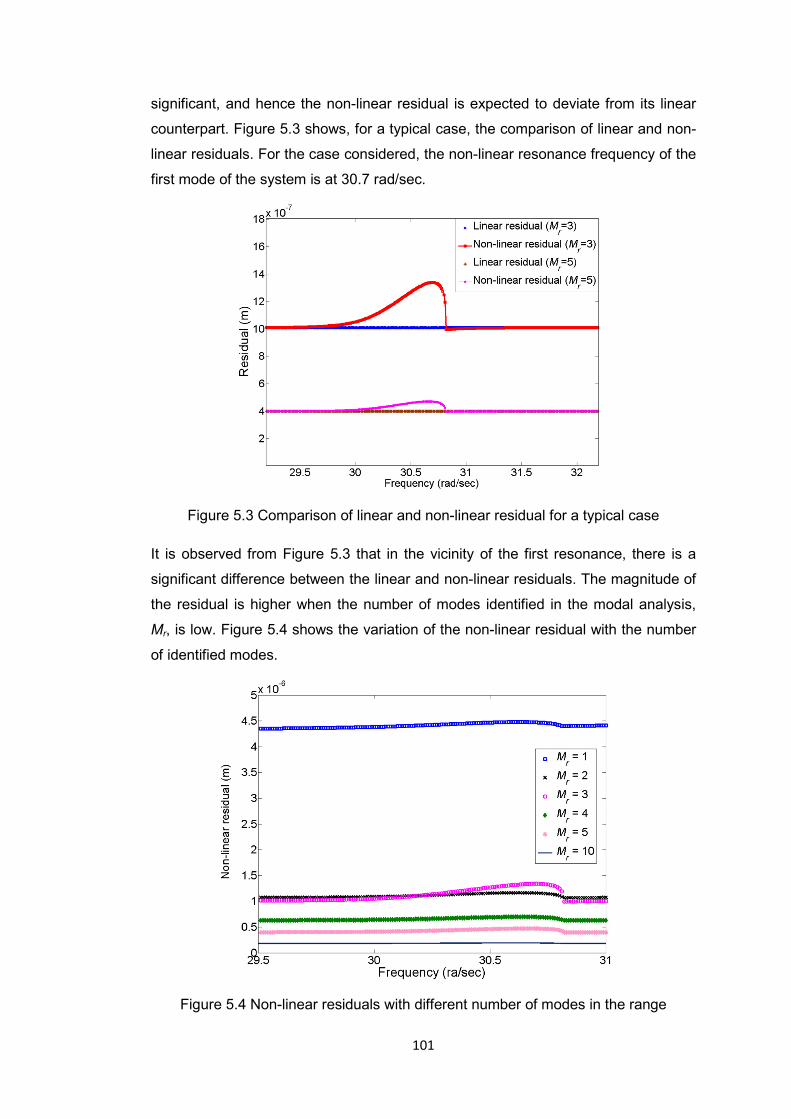
101
significant, and hence the non-linear residual is expected to deviate from its linear
counterpart. Figure 5.3 shows, for a typical case, the comparison of linear and non-
linear residuals. For the case considered, the non-linear resonance frequency of the
first mode of the system is at 30.7 rad/sec.
Figure 5.3 Comparison of linear and non-linear residual for a typical case
It is observed from Figure 5.3 that in the vicinity of the first resonance, there is a
significant difference between the linear and non-linear residuals. The magnitude of
the residual is higher when the number of modes identified in the modal analysis,
Mr, is low. Figure 5.4 shows the variation of the non-linear residual with the number
of identified modes.
Figure 5.4 Non-linear residuals with different number of modes in the range
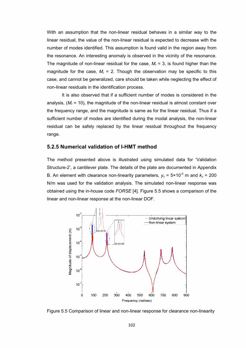
102
With an assumption that the non-linear residual behaves in a similar way to the
linear residual, the value of the non-linear residual is expected to decrease with the
number of modes identified. This assumption is found valid in the region away from
the resonance. An interesting anomaly is observed in the vicinity of the resonance.
The magnitude of non-linear residual for the case, Mr = 3, is found higher than the
magnitude for the case, Mr = 2. Though the observation may be specific to this
case, and cannot be generalized, care should be taken while neglecting the effect of
non-linear residuals in the identification process.
It is also observed that if a sufficient number of modes is considered in the
analysis, (Mr = 10), the magnitude of the non-linear residual is almost constant over
the frequency range, and the magnitude is same as for the linear residual. Thus if a
sufficient number of modes are identified during the modal analysis, the non-linear
residual can be safely replaced by the linear residual throughout the frequency
range.
5.2.5 Numerical validation of I-HMT method
The method presented above is illustrated using simulated data for ‘Validation
Structure-2’, a cantilever plate. The details of the plate are documented in Appendix
B. An element with clearance non-linearity parameters, yc = 5×10⁻⁵ m and kz = 200
N/m was used for the validation analysis. The simulated non-linear response was
obtained using the in-house code FORSE [4]. Figure 5.5 shows a comparison of the
linear and non-linear response at the non-linear DOF.
Figure 5.5 Comparison of linear and non-linear response for clearance non-linearity

103
It is seen from Figure 5.5 that the first two modes are affected most by the non-
linearity and the rest of the modes behave almost linearly.
Pre-processing stage The underlying linear modal model was obtained by performing modal analysis on
the structure to extract the modal properties for the first nine modes (Mr = 9). The
displacement responses were captured at 16 locations uniformly distributed over the
plate (m = 16). As it is difficult to measure the rotational DOFs in practical cases, all
16 responses are the translational displacements along Z axis. The details of the
available modal model and the non-linear response measurements are given below.
The numbers below indicate the node number followed by a letter indicating the
DOF at the node, X for the rotation about X axis, Y for the rotation about Y axis and
Z for the translation along Z axis. The information is also depicted in Figure 5.6 for a
better illustration of the process.
Measured DOFs (Z translational): {1, 3, 5, 7, 11, 13, 15, 17, 21, 23, 25, 27, 29, 32,
37, 42} Un-measured DOFs: {1X-42X; 1Y-42Y; 2Z, 4Z, 6Z, 8Z-10Z, 12Z, 14Z, 16Z, 18Z-
20Z, 22Z, 24Z, 26Z, 28Z, 30Z, 31Z, 33Z-36Z, 38Z-41Z}
Excitation force applied at: {37Z} Excitation force amplitude = 0.01N
Non-linear element incorporated at: {42Z}
Identified modes from linear modal analysis: {1, 2, 3..., 9}
Figure 5.6 Details of the measured locations

104
Extraction of the non-linear modal vector (NMV)
The non-linear modal vector was extracted using (5.12). Out of the first nine modes
which were identified in the modal analysis, only the first two modes behave non-
linearly. Owing to this, the non-linear residual value around the non-linear
resonances was assumed to be small. Thus the non-linear residual was replaced by
the linear residual. Figure 5.7 shows the plot of the amplitude of non-linear modal
vector for the first mode. The top part of the figure shows the non-linear response at
the non-linear DOF, and the bottom part of the figure shows the amplitude of non-
liner modal vector for the first mode plotted in the same frequency range as the non-
linear response. The dashed line in the bottom plot shows the linear threshold for
the first mode. It can be observed from the plot that the NMV crosses the linear
threshold for the first two resonances. Figure 5.8 shows a zoomed-in view of the
NMV in the vicinity of the first resonance.
Figure 5.7 Extracted non-linear modal vector for the first mode
Once the NMVs were extracted for the identified modes, the non-linear modal grade
(NMG) was calculated for each mode using (5.13) to decide on the modes to be
retained in further analysis. Figure 5.9 shows a bar chart for NMGs for the first five
modes. It is seen that the NMGs for the first two modes are greater than that for the
other modes. Thus, the first two modes are classified as the non-linear modes, and
the points in the vicinity of the first two resonances are selected while formulating
the optimization problem.
0 100 200 300 400 500 600 700 80010-8
10-6
10-4
10-2
Dis
plac
emen
t am
plitu
de (m
)
0 100 200 300 400 500 600 700 800
0.2
0.4
0.6
Frequency (rad/sec)
( φT G
) 1
Non-linear modal vectorLinear threshold

105
Figure 5.8 Zoomed-in view of NMV near the first resonance
Figure 5.9 Non-linear modal grades for the modes in the measurement range
Estimation of the non-linear parameters
The optimization problem was solved using a GA to extract the non-linear
parameters. The values of the control parameters, like the population size, the
number of generations, and the probability of cross-over operator were kept same
as those in Table 4.1. The range for the non-linear parameters used in the first
civilization is as follows:
Gap distance, yc,: (1×10⁻⁷-1×10⁻⁴) m.
Clearance stiffness, Kz: (0-400) N/m
Initially (Case A), the optimization problem was formulated with all measured
DOFs, simulating the case where the non-linear location is not identified a-priori.
The total number of non-linear parameters to be identified is 80. For this case, the
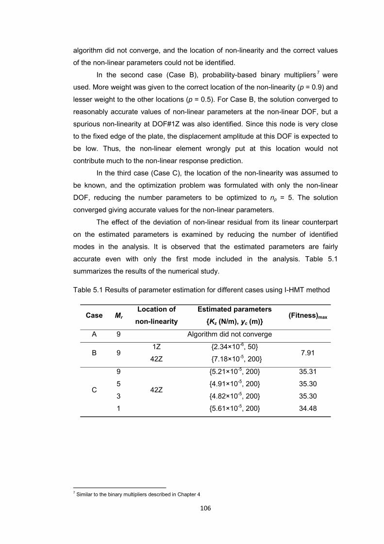
106
algorithm did not converge, and the location of non-linearity and the correct values
of the non-linear parameters could not be identified.
In the second case (Case B), probability-based binary multipliers 7 were
used. More weight was given to the correct location of the non-linearity (p = 0.9) and
lesser weight to the other locations (p = 0.5). For Case B, the solution converged to
reasonably accurate values of non-linear parameters at the non-linear DOF, but a
spurious non-linearity at DOF#1Z was also identified. Since this node is very close
to the fixed edge of the plate, the displacement amplitude at this DOF is expected to
be low. Thus, the non-linear element wrongly put at this location would not
contribute much to the non-linear response prediction.
In the third case (Case C), the location of the non-linearity was assumed to
be known, and the optimization problem was formulated with only the non-linear
DOF, reducing the number parameters to be optimized to np = 5. The solution
converged giving accurate values for the non-linear parameters.
The effect of the deviation of non-linear residual from its linear counterpart
on the estimated parameters is examined by reducing the number of identified
modes in the analysis. It is observed that the estimated parameters are fairly
accurate even with only the first mode included in the analysis. Table 5.1
summarizes the results of the numerical study.
Table 5.1 Results of parameter estimation for different cases using I-HMT method
Case Mr Location of
non-linearity Estimated parameters
{Kz (N/m), yc (m)} (Fitness)max
A 9 Algorithm did not converge
B 9 1Z
42Z
{2.34×10⁻⁶, 50}
{7.18×10⁻⁵, 200} 7.91
C
9
42Z
{5.21×10⁻⁵, 200} 35.31
5 {4.91×10⁻⁵, 200} 35.30
3 {4.82×10⁻⁵, 200} 35.30
1 {5.61×10⁻⁵, 200} 34.48
7 Similar to the binary multipliers described in Chapter 4

107
5.3 FRF-based method
The I-HMT method presented in Section 5.2 uses the modal model of the underlying
linear system, which can be obtained by performing modal analysis on the raw FRF
measurements. There are two limitations of the I-HMT method:
(i) The non-linearity must be correctly located and the non-linear DOF must
be measured for efficient working of the optimization algorithm.
(ii) The modal analysis of measured data can introduce additional errors if it
is not performed carefully.
The method proposed in this section uses the raw FRF measurements
directly to extract the non-linear restoring force. On the one hand, if the non-linear
DOFs are located and measured, the method extracts the non-linear force at these
non-linear DOFs. On the other hand, if there is a localized non-linearity at a single
point, which is located but not measured, the method uses a technique to
approximate the non-linear restoring force at the non-linear DOF.
As the FRF matrix for a linear system is symmetric, it is not necessary to
obtain the complete FRF matrix through experiments, thus reducing the costs
related to the experimentation. The method completely relies on measured data,
making it useful when the accurate FE model and sophisticated modal analysis
tools are not available.
5.3.1 Theoretical formulation
In the frequency domain, the equations of motion for an MDOF non-linear system
under harmonic excitation are written as:
[ ] [ ] [ ]( ){ } { } { }FYGYDiKM =+++− ),(2 ωω (5.21)
The quantity inside the curved brackets on the left-hand side of (5.21) is defined as
the dynamic stiffness matrix of the system, denoted by[ ]Z . The FRF matrix for a
system, [ ]α , is defined as the inverse of the dynamic stiffness matrix. Pre-multiplying
(5.21) by the FRF matrix we get
{ } [ ]{ } [ ]{ }FGY αα =+ (5.22)
If subscript m denotes the measured DOFs and subscript u denotes the un-
measured DOFs of the system, (5.22) can be partitioned as:

108
⎭⎬⎫
⎩⎨⎧⎥⎦
⎤⎢⎣
⎡=
⎭⎬⎫
⎩⎨⎧⎥⎦
⎤⎢⎣
⎡+
⎭⎬⎫
⎩⎨⎧
u
m
uuum
mumm
u
m
uuum
mumm
u
m
FF
GG
YY
αααα
αααα
(5.23)
If the displacements at the measured DOFs are considered, the system of
equations can be written as:
{ } [ ]{ } [ ]{ } [ ]{ } [ ]{ }umummmumummmm FFGGY αααα +=++ (5.24)
If it is assumed that all excitation DOFs are measured, a condition which can be
easily achieved during controlled experimentation, the vector {Fu} becomes zero.
Substituting {Fu} = 0 in (5.24), and multiplying by [ ] 1−mmα ,
{ } { } [ ] { }{ }
[ ] [ ]{ }( )umumm
G
mmmmm GYFG ααα 11
0
−− −−=444 3444 21 (5.25)
Rearranging (5.25) we get
{ } { } [ ] [ ]{ }( )umummm GGG αα 10 −+= (5.26)
where, { }0G denotes the term in (5.25) which can be extracted using available
measurements. In a special case where all non-linear DOFs are measured,
{ } 0=uG , and { }0G gives the non-linear restoring force vector at the measured
DOFs:
{ } { } { } [ ] { }mmmmm YFGG 10 −−== α (5.27)
Equation (5.27) gives the expression for the non-linear restoring force at the
measured DOFs when all excitation DOFs and all non-linear DOFs are measured.
This is an exact equation with no approximations or truncations if it is used within
the above constraints.
In many practical cases, the location of non-linearity is physically
inaccessible, and a measurement cannot be made at that location. However, if there
is a location close to the non-linearity location where the measurement can be
taken, the non-linear restoring force at the non-linear DOF can be extracted
indirectly. Let subscript c denotes the location close to the non-linear DOF at
which the measurement is taken, subscript e denotes the excitation DOF, and
subscript nl denotes the non-linear DOF, which is not measured. If all measured

109
DOF are linear,{ } 0=mG . If the FRF matrix is constructed using the excitation DOF
and the DOF close to the non-linearity location only, (5.26) can be expanded as:
{ } [ ]{ }( )umueeec
cecc GG ααααα 1
0−
⎥⎦
⎤⎢⎣
⎡= (5.28)
For a localized non-linearity at the nl th DOF, only the corresponding value in the
vector {Gu} would be non-zero. Thus, rewriting (5.28)
{ }⎭⎬⎫
⎩⎨⎧
⎥⎦
⎤⎢⎣
⎡=
−
nlenl
nlcnl
eeec
cecc
GG
Gαα
αααα 1
0 (5.29)
The two entries in vector G0 can be explicitly written as:
nlceecccee
enlcecnlee GG ⎟⎟⎠
⎞⎜⎜⎝
⎛−−
=αααααααα0
1 (5.30a)
nlceecccee
cnlecenlcc GG ⎟⎟⎠
⎞⎜⎜⎝
⎛−−
=αααααααα0
2 (5.30b)
If the measured location c is sufficiently close to the non-linear location, then for
lower modes where the structural deformation is not localized, location c can be
replaced by the non-linear location nl in the FRF matrix. Thus, replacing enlα by ecα
, and cnlα by ccα in (5.30a) and (5.30b) and adding the two equations we get:
( )02
01 GGGnl +≈ (5.31)
Thus, an approximate expression for the non-linear force at the non-linear DOF can
be obtained using the measurement closest to the non-linearity location. This
expression is only valid in the case of single point excitation and a single localized
non-linearity in the system.
5.3.2 Conditioning of the FRF matrix
The condition number of a matrix is mathematically expressed as the ratio of its
largest singular value to its smallest non-zero singular value [7]. A high value of the
condition number represents an ill-conditioned matrix. The inversion of an ill-
conditioned matrix can be inaccurate, thus it should be avoided.
The expression for the non-linear force vector in (5.25) involves an inversion
of the part of the FRF matrix containing the measured DOFs. The value of condition
number of the FRF matrix is a function of different parameters like the excitation
frequency, damping in the system, the number of measurements, and locations of
measurements. Figure 5.10 shows the variation of the condition number of an FRF
matrix in a typical case. It is observed that the condition number varies with the

110
excitation frequency, and attains a maximum value near the resonance frequency of
the system. The maximum value of the condition number is higher for lightly
damped systems. The maximum value also increases with the size of the FRF
matrix.
Figure 5.10 Variation of the condition number of the FRF matrix
The condition number of the FRF matrix is also dependent on the selection of the
measured DOFs. For a fixed number of measurements, it is observed that if only the
translational measurements are distributed uniformly over the structure, the
condition number is the lowest. On the other side if the translational and rotational
DOFs are combined in the FRF matrix, the condition number is highest. Figure 5.11
shows the effect of the location of the measurements on the condition number of the
FRF matrix.
Figure 5.11 Effect of measurement locations on the condition number
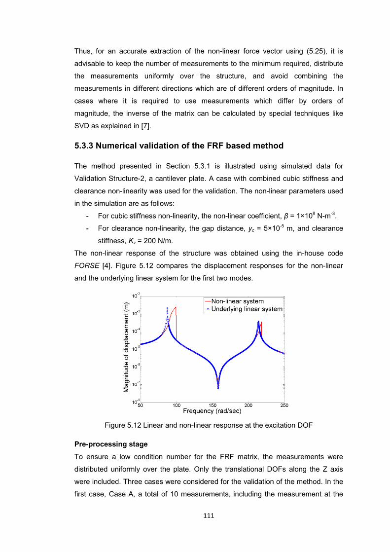
111
Thus, for an accurate extraction of the non-linear force vector using (5.25), it is
advisable to keep the number of measurements to the minimum required, distribute
the measurements uniformly over the structure, and avoid combining the
measurements in different directions which are of different orders of magnitude. In
cases where it is required to use measurements which differ by orders of
magnitude, the inverse of the matrix can be calculated by special techniques like
SVD as explained in [7].
5.3.3 Numerical validation of the FRF based method
The method presented in Section 5.3.1 is illustrated using simulated data for
Validation Structure-2, a cantilever plate. A case with combined cubic stiffness and
clearance non-linearity was used for the validation. The non-linear parameters used
in the simulation are as follows:
- For cubic stiffness non-linearity, the non-linear coefficient, β = 1×10⁸ N-m-3.
- For clearance non-linearity, the gap distance, yc = 5×10⁻⁵ m, and clearance
stiffness, Kz = 200 N/m.
The non-linear response of the structure was obtained using the in-house code
FORSE [4]. Figure 5.12 compares the displacement responses for the non-linear
and the underlying linear system for the first two modes.
Figure 5.12 Linear and non-linear response at the excitation DOF
Pre-processing stage
To ensure a low condition number for the FRF matrix, the measurements were
distributed uniformly over the plate. Only the translational DOFs along the Z axis
were included. Three cases were considered for the validation of the method. In the
first case, Case A, a total of 10 measurements, including the measurement at the
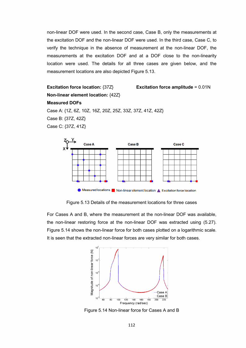
112
non-linear DOF were used. In the second case, Case B, only the measurements at
the excitation DOF and the non-linear DOF were used. In the third case, Case C, to
verify the technique in the absence of measurement at the non-linear DOF, the
measurements at the excitation DOF and at a DOF close to the non-linearity
location were used. The details for all three cases are given below, and the
measurement locations are also depicted Figure 5.13.
Excitation force location: {37Z} Excitation force amplitude = 0.01N
Non-linear element location: {42Z}
Measured DOFs Case A: {1Z, 6Z, 10Z, 16Z, 20Z, 25Z, 33Z, 37Z, 41Z, 42Z}
Case B: {37Z, 42Z}
Case C: {37Z, 41Z}
Figure 5.13 Details of the measurement locations for three cases
For Cases A and B, where the measurement at the non-linear DOF was available,
the non-linear restoring force at the non-linear DOF was extracted using (5.27).
Figure 5.14 shows the non-linear force for both cases plotted on a logarithmic scale.
It is seen that the extracted non-linear forces are very similar for both cases.
Figure 5.14 Non-linear force for Cases A and B

113
For Case C, since the non-linear DOF was not measured, (5.30) was used to
extract the non-linear force components, G01 and G0
2, at the measured DOFs.
Finally the two components were summed up to find the approximate value of non-
linear force at the non-linear DOF. In Figure 5.15, the plot on the left shows the non-
linear forces at the measured DOFs, and the plot on the right compares the
summed non-linear force with the non-linear force for Case A. It is seen that
approximated non-linear force for Case C is in close agreement with the actual non-
linear force.
Figure 5.15 Extraction of the non-linear force for Case C
For Cases A and B, the extracted non-linear force was expressed as a
function of the displacement at the non-linear DOF. For Case C, the approximated
non-linear force was expressed as a function of the displacement at the DOF close
to the non-linear DOF. The non-linear parameters were identified using the genetic
algorithm optimization presented in Chapter 4. For the initial civilization, the range
for β was kept as (0-1×10¹⁰) Nm-3, for yc, was kept as (0-5×10⁻⁴) m and for Kz, was
kept as (0-800) N/m. Later, the range was narrowed down to increase the accuracy
of parameter estimation. The final values of the estimated non-linear parameters are
summarised in Table 5.2.
Table 5.2 Summary of the parameter identification results using FRF-based method
Case Max. Cond.
number Identified parameters
{β (Nm-3), yc (m), Kz (N/m)} Error (%)
{εβ, εyc, εkz} Fitness
A 2.78×10⁵ {1.002×10⁸, 5.36×10⁻⁵, 200} {0.2, 7.2, 0} 99.36
B 550.7 {1.003×10⁸, 5.23×10⁻⁵, 200} {0.3, 4.6, 0} 98.73
C 841.6 {7.212×10⁷, 9.62×10⁻⁵, 225} {27.9, 92.4, 12.5} 95.31

It is observed that the
less than 8%. For
absence of the meas
observed that for Ca
parameters are accu
at the excitation DO
that even for Case C
more than 40%, the d
around 4-5%. It sugg
non-linear parameter
Figure 5.16 Comparis
the FRF-based metho
114
e maximum error in parameter estimation fo
Case C, where the non-linear parameters
surement at non-linear location, the error is h
ase A, though the condition number is in th
urately identified. Figure 5.16 shows the reg
F with the identified parameters for all three
C, where the average error in the estimatio
deviations in resonance frequency and reson
gests that the response difference has differ
rs.
son of the accurate response and the regene
od predictions
r Cases A and B is
s are identified in
high. It can be also
e order of 105, the
enerated response
e cases. It is seen
on of parameters is
nance response are
rent sensitivities for
erated response for
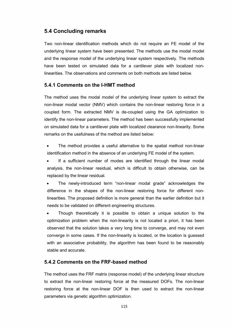
115
5.4 Concluding remarks
Two non-linear identification methods which do not require an FE model of the
underlying linear system have been presented. The methods use the modal model
and the response model of the underlying linear system respectively. The methods
have been tested on simulated data for a cantilever plate with localized non-
linearities. The observations and comments on both methods are listed below.
5.4.1 Comments on the I-HMT method
The method uses the modal model of the underlying linear system to extract the
non-linear modal vector (NMV) which contains the non-linear restoring force in a
coupled form. The extracted NMV is de-coupled using the GA optimization to
identify the non-linear parameters. The method has been successfully implemented
on simulated data for a cantilever plate with localized clearance non-linearity. Some
remarks on the usefulness of the method are listed below:
• The method provides a useful alternative to the spatial method non-linear
identification method in the absence of an underlying FE model of the system.
• If a sufficient number of modes are identified through the linear modal
analysis, the non-linear residual, which is difficult to obtain otherwise, can be
replaced by the linear residual.
• The newly-introduced term “non-linear modal grade” acknowledges the
difference in the shapes of the non-linear restoring force for different non-
linearities. The proposed definition is more general than the earlier definition but it
needs to be validated on different engineering structures.
• Though theoretically it is possible to obtain a unique solution to the
optimization problem when the non-linearity is not located a priori, it has been
observed that the solution takes a very long time to converge, and may not even
converge in some cases. If the non-linearity is located, or the location is guessed
with an associative probability, the algorithm has been found to be reasonably
stable and accurate.
5.4.2 Comments on the FRF-based method
The method uses the FRF matrix (response model) of the underlying linear structure
to extract the non-linear restoring force at the measured DOFs. The non-linear
restoring force at the non-linear DOF is then used to extract the non-linear
parameters via genetic algorithm optimization.

116
• It has been observed that the measurements at the non-linear DOFs and the
excitation DOF are sufficient to accurately identify the non-linear parameters.
This significantly reduces the size of the problem for practical cases.
• If the response at the non-linear DOF is not available, a technique has been
presented to approximate the non-linear restoring force at the non-linear DOF
using the measurement at a location close to the non-linearity location. This
technique has reduced accuracy in comparison to the original technique.
The method has been successfully validated on simulated data for a cantilever plate
with combined cubic stiffness and clearance non-linearity.

117
Chapter 6
Comparison of non-linear parameter identification methods
This chapter presents a comparative study of three methods for non-linear system
identification, presented in Chapters 4 and 5. The study is carried out on the so-
called ‘1203 structure’, which can be considered as a representative engineering
structure. Simulated non-linear response data and numerical models of the
underlying linear structure are used as input to the parameter identification. Two
cases of increasing complexity are considered: (i) an idealized cubic stiffness non-
linearity and (ii) a realistic clearance non-linearity. The methods are compared on
the basis of different evaluation criteria like: accuracy of parameter estimation,
sensitivity to measurement noise, sensitivity to errors in the input model, ability to
locate the non-linearity, performance with partial measurement set, and
computational efficiency.
6.1 Introduction
The methods presented in Chapters 4 and 5, for non-linear system identification,
can potentially be used to tackle large multi-degrees of freedom (MDOFs) systems
of practical interest. Each method requires different input, and it has its own
advantages and limitations. Table 6.1 gives the summary of input requirements for
the three methods. The methods have been illustrated on simple structures before,
but it is necessary to compare their performance on common grounds, using data
obtained for a representative engineering structure.

118
Table 6.1 Details of the three methods compared
Method name Method number
Input requirement
Spatial method 1 Updated FE model of the
underlying linear system
Improved hybrid modal
technique (I-HMT) 2
Modal model of the
underlying linear system
FRF-based method 3 Response model of the
underlying linear system
It can be argued that actual experimental data obtained for a practical non-linear
structure should be used for comparing the identification methods. However, in case
of non-linear structures, the use of experimental data poses many additional
difficulties, some of which are as follows:
(i) Obtaining consistent and repeatable vibration measurements on a non-linear
structure is a challenging task.
(ii) In practical non-linear structures, the non-linearities may not behave as per
their idealized mathematical formulation.
(iii) The actual values of the non-linear parameters are unknown in practical
cases, making the comparison of different methods difficult because of a lack
of reference data.
The methods presented in the earlier chapters work within certain assumptions like
the idealized mathematical formulation for different non-linear elements, the use of
first-order describing functions to represent the non-linear force etc. The objective of
the work presented in this chapter is to compare the three identification methods
based on their accuracy and robustness within these assumptions. Thus, it is more
appropriate to use simulated data for the comparison.
The so-called ‘1203 structure’ is used for the comparison. This structure,
based on the outer cover geometry of an electrical component, was used as the
benchmark structure for validating linear modal analysis algorithms in the MODENT
software in ICATS [117]. The same structure, with some alterations to the
dimensions, is used. The detailed engineering drawings of the 1203 structure, as
used in this study, are given in Appendix C.
The underlying linear structure was modelled in ANSYS using shell elements
(SHELL63) to mesh the surfaces and 3D beam elements (BEAM4) to mesh the two
stiffening beams. All elements used possess 6 DOFs per node. The structure was

119
assumed to be bolted to a fairly rigid structure, which could be treated as ground, at
the locations of two holes. The excitation force of amplitude 0.1N was applied at one
corner of the structure acting in positive X direction. Figure 6.1 shows the computer
model, and the meshed model with boundary conditions for the structure.
Figure 6.1 CAD and FE models ‘1203 structure’
6.2 Test cases for the comparison
Two test cases of increasing complexity are considered in this chapter for the
comparison of the methods. The first case, Case A, uses a grounded cubic stiffness
non-linearity at one end of the lower beam. This is an idealized case used to
evaluate the performance of the methods with a complex structure. The second
case, Case B, implements a realistic clearance non-linearity. A rubber block, 4×4
cm in cross-section and 5cm thick, is placed adjacent to the structure with a small
clearance between the block and the structure. During the vibration of the structure,
the structure will hit the rubber block, thus producing clearance non-linearity. In the
simulation, this condition was approximated by using four clearance elements
distributed over the patch spanning the rubber block. Figure 6.2 shows, in front
view, the location of non-linearities in both cases. The details of non-linearity
locations and the parameters used to simulate the non-linearities are given in Table
6.2.
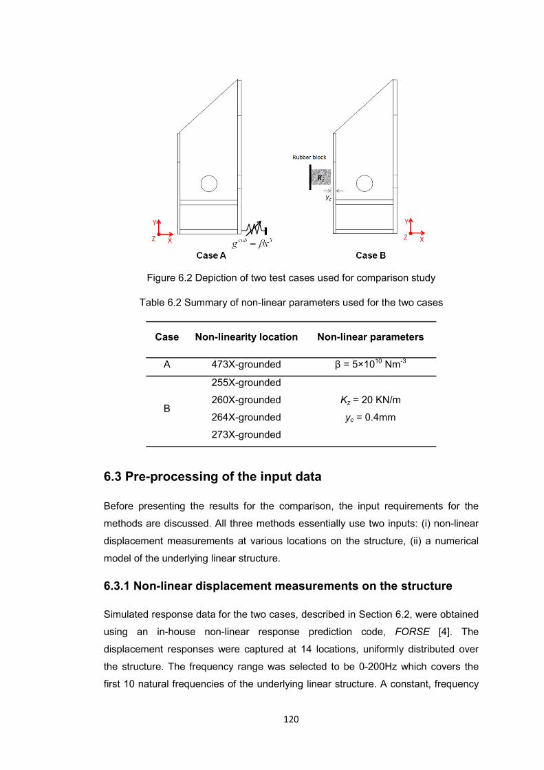
120
Figure 6.2 Depiction of two test cases used for comparison study
Table 6.2 Summary of non-linear parameters used for the two cases
Case Non-linearity location Non-linear parameters
A 473X-grounded β = 5×10¹⁰ Nm-3
B
255X-grounded
Kz = 20 KN/m
yc = 0.4mm
260X-grounded
264X-grounded
273X-grounded
6.3 Pre-processing of the input data
Before presenting the results for the comparison, the input requirements for the
methods are discussed. All three methods essentially use two inputs: (i) non-linear
displacement measurements at various locations on the structure, (ii) a numerical
model of the underlying linear structure.
6.3.1 Non-linear displacement measurements on the structure
Simulated response data for the two cases, described in Section 6.2, were obtained
using an in-house non-linear response prediction code, FORSE [4]. The
displacement responses were captured at 14 locations, uniformly distributed over
the structure. The frequency range was selected to be 0-200Hz which covers the
first 10 natural frequencies of the underlying linear structure. A constant, frequency
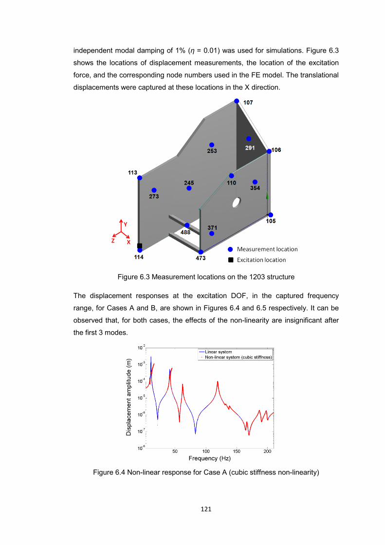
121
independent modal damping of 1% (η = 0.01) was used for simulations. Figure 6.3
shows the locations of displacement measurements, the location of the excitation
force, and the corresponding node numbers used in the FE model. The translational
displacements were captured at these locations in the X direction.
Figure 6.3 Measurement locations on the 1203 structure
The displacement responses at the excitation DOF, in the captured frequency
range, for Cases A and B, are shown in Figures 6.4 and 6.5 respectively. It can be
observed that, for both cases, the effects of the non-linearity are insignificant after
the first 3 modes.
Figure 6.4 Non-linear response for Case A (cubic stiffness non-linearity)

122
Figure 6.5 Non-linear response for Case B (clearance non-linearity)
Later in the analysis, to evaluate the effects of measurement noise on the accuracy
of parameter estimation, the responses were polluted with 5% random noise using
(4.15) from Chapter 4.
6.3.2 Input models for different methods
The three methods which are compared in this chapter require a numerical model of
the underlying linear structure in different forms. The extent of possible errors in the
input models of these methods may also differ in practice. For example, an FE
model which is used in one method may be more prone to errors than a response
model which is required for the other method. The following section discusses
different numerical models which are used as the input for the three methods. It also
states the sources and the extent of errors in these models. The levels of errors, at
which the methods are to be tested, are decided based on the engineering
judgement so as to make a fair comparison.
The spatial method for non-linear parameter identification, presented in
Chapter 4, is referred to as ‘Method 1’ in further discussion for the purpose of
brevity. The finite element matrices of the underlying linear structure are used as the
input to this method. The errors in FE models can come from the uncertainties in
material properties and joint stiffness, or the tolerances on physical dimensions. To
evaluate the effect of errors in the input data, it was decided to change the material
properties. The Young’s modulus of elasticity and the density of the material in the
FE model were increased by 4.5% and 3.5% respectively. This resulted in

123
approximately 1-2% change in the first few natural frequencies. This level of
accuracy in FE models can arguably be attained in the updated FE models.
The improved hybrid modal technique (I-HMT), presented in Chapter 5, is
referred to as ‘Method 2’ in further discussion. The modal model of the underlying
linear structure serves as the input model for this method. Modal models, which are
extracted via an experimental route, are usually incomplete. For the current study, a
modal model with the first ten modes (Mr = 10), and measurements at 14 locations
on the structure (m = 14) was used. The condition, m ≥ Mr, required for extracting
the non-linear modal vector was met while selecting the modal model. Though the
modal analysis tools are well established, only the first few modes are generally
identified with good accuracy. Thus, errors in a modal model may arise from the
errors in the estimation of modal properties of higher modes of the system. To study
the effects of errors in the input model, the natural frequencies and mode shape
vectors for identified modes were polluted with a random error of up to 3%. The
lower modes, which are generally identified with good accuracy, were polluted with
less error.
The FRF based method, presented in Chapter 5, is referred to as ‘Method 3’
in further discussion. The measured FRF matrix of the underlying linear structure is
used as the input to this method. To evaluate the effects of errors in the input model
on parameter estimation, the FRF measurements were polluted with 5% random
noise. The polluted FRF matrix at each frequency line was calculated using (6.1)
)()100/1()( ωαωα ijp
ij cr ×±= (6.1)
where, r is a random number (0 ≤ r ≤1),
c is the maximum level of noise in percentage,
pijα and ijα are the components of FRF matrix with and without noise
respectively.
6.4 Results of non-linear parameter identification for Case A
The three methods were used successively to identify the non-linear parameters for
Case A, with cubic stiffness non-linearity. As, the response beyond 50Hz was
consistently linear, the frequency range was restricted to 50Hz. Firstly, a clean non-
linear displacement response and accurate input models for the three methods were
used to identify the non-linear parameters. Methods 1 and 3 were used extract the
non-linear force vector, which helps to identify the location of the non-linearity.

124
Method 2 was used to extract the values of non-linear parameters directly. For
Methods 1 and 3, the accumulated non-linear force at the measured DOFs was
calculated to locate the non-linearity.
Figure 6.6 shows a plot of the accumulated non-linear force. It is observed
that the non-linearity location is correctly identified at node#473 using both methods.
Figure 6.7 shows the comparison of the magnitude of non-linear force at the non-
linear DOF for Methods 1 and 3.
Figure 6.6 Identification of the location of non-linearity for Case A
Figure 6.7 Non-linear force at the non-linear DOF for Case A
It can be observed that the values of non-linear force extracted using the two
methods differ significantly at the anti-resonances. The values match closely in the
vicinity of the resonances. As explained in Chapters 4 and 5, the points in the

125
vicinity of resonances are to be selected to form the optimization problem. Thus, the
difference in the values at anti-resonances will not affect the identification results.
For Method 2, the non-linear modal vector was extracted for the measured
modes. This vector implicitly stores the information about non-linear parameters.
Figure 6.8 shows the plot of non-linear modal vector for the second mode and the
corresponding linear-threshold.
Figure 6.8 Non-linear modal vector plotted for Case A
It is observed that, in the vicinity of the second and the third resonances, the NMV
exceeds the linear threshold value. In the vicinity of the first mode, the NMV is
consistently below the linear threshold. This indicates that the first mode is behaving
linearly while the effect of non-linearity is dominant in the second and the third
modes.
Figure 6.9 Non-linear modal grade (NMG) plot for Case A
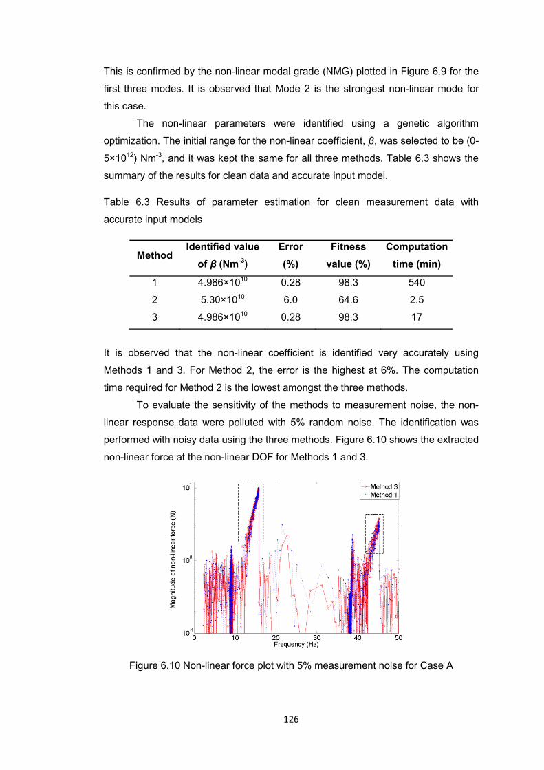
126
This is confirmed by the non-linear modal grade (NMG) plotted in Figure 6.9 for the
first three modes. It is observed that Mode 2 is the strongest non-linear mode for
this case.
The non-linear parameters were identified using a genetic algorithm
optimization. The initial range for the non-linear coefficient, β, was selected to be (0-
5×10¹²) Nm-3, and it was kept the same for all three methods. Table 6.3 shows the
summary of the results for clean data and accurate input model.
Table 6.3 Results of parameter estimation for clean measurement data with
accurate input models
Method Identified value
of β (Nm-3) Error (%)
Fitness value (%)
Computation time (min)
1 4.986×10¹⁰ 0.28 98.3 540
2 5.30×10¹⁰ 6.0 64.6 2.5
3 4.986×10¹⁰ 0.28 98.3 17
It is observed that the non-linear coefficient is identified very accurately using
Methods 1 and 3. For Method 2, the error is the highest at 6%. The computation
time required for Method 2 is the lowest amongst the three methods.
To evaluate the sensitivity of the methods to measurement noise, the non-
linear response data were polluted with 5% random noise. The identification was
performed with noisy data using the three methods. Figure 6.10 shows the extracted
non-linear force at the non-linear DOF for Methods 1 and 3.
Figure 6.10 Non-linear force plot with 5% measurement noise for Case A

127
It can be observed that the extracted non-linear force plot is extremely noisy in the
region away from the resonances. The non-linear force values in the vicinity of
resonances, indicated by the rectangular boxes in Figure 6.10, were used to identify
the non-linear parameters. The non-linear modal vector (NMV) was extracted using
Method 2. Figure 6.11 shows the plot of the NMV for the 2nd mode in the vicinity of
the 2nd resonance. The summary of parameter estimation is given in Table 6.4.
Figure 6.11 NMV for the 2nd mode plotted for Case A with noise
Table 6.4 Estimated non-linear parameter with noise for Case A
Method Identified value of β
(Nm-3) Error (%)
Fitness value (%)
1 5.242×10¹⁰ 4.84 6.5
2 5.738×10¹⁰ 14.76 20.3
3 5.197×10¹⁰ 3.94 7.7
It is observed that the errors in the estimated parameter using Methods 1 and 3 are
comparable, and are less than 5%. The error in the estimated parameter using
Method 2 is the highest. The fitness value of the objective function used in the
optimization process is consistently low for all three methods when compared to the
fitness value in case of noise-free identification (Table 6.2). The low fitness value is
consistent with the fact that the parameters are identified from noisy data.
To access the performance of the methods with erroneous input models, the
corresponding input models for the three methods were polluted with artificial errors
as explained in Section 6.3.2. The noise-free responses were used in this case.

128
Table 6.5 summarizes the estimated parameters for the case of erroneous input
models.
Table 6.5 Estimated non-linear parameter with erroneous input models for Case A
Method Identified value of β
(Nm-3) Error (%)
Fitness value (%)
1 5.195×10¹⁰ 3.90 83.9
2 4.353×10¹⁰ 12.93 55.6
3 4.819×10¹⁰ 3.62 7.8
It is observed that Methods 1 and 3 yield accurate values of non-linear parameter
even with inaccurate input models. Method 2 identifies the non-linear parameter
with around 13% error.
6.4 Results of non-linear parameter identification for Case B
In the second part of the comparison, a more practical case with distributed
clearance non-linearity is considered. It is seen from Figure 6.5 that the non-linearity
is affecting the response up to 50Hz only. Thus, the frequency range was restricted
to 0-50 Hz, covering the first three modes, for the identification exercise.
The displacement response for this case was simulated using four clearance
non-linearity elements distributed over the contact area. For the identification of
non-linear parameters, the non-linear responses were captured at the same 14
locations as described in Section 6.3.1. It is interesting to note that the
measurement was taken at only one out of the four nodes (Node 273), at which the
non-linear elements were incorporated. Since all non-linear DOFs were not
measured, it was not possible to identify the actual values of parameters which were
used to simulate the displacement response. Instead, the equivalent non-linear
parameters at the measured DOF were identified. This made it difficult to evaluate
the accuracy of the methods, which was done earlier by direct comparison of the
identified and actual non-linear parameters.
In this case, the accuracy of different methods was evaluated from the
predicted non-linear displacement response using identified equivalent parameters.
The error was specified in terms of deviation in the resonant response and the
resonance frequency of the strongest non-linear mode.
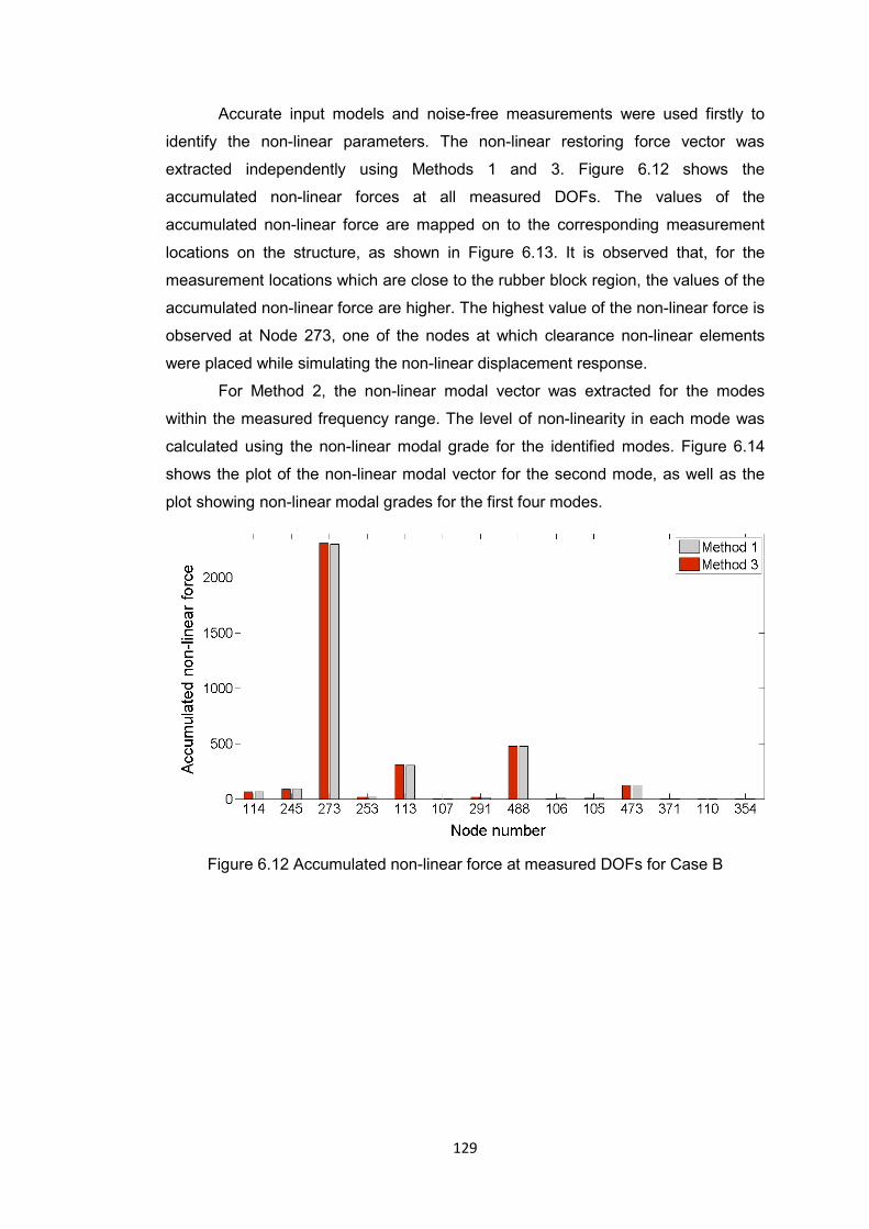
129
Accurate input models and noise-free measurements were used firstly to
identify the non-linear parameters. The non-linear restoring force vector was
extracted independently using Methods 1 and 3. Figure 6.12 shows the
accumulated non-linear forces at all measured DOFs. The values of the
accumulated non-linear force are mapped on to the corresponding measurement
locations on the structure, as shown in Figure 6.13. It is observed that, for the
measurement locations which are close to the rubber block region, the values of the
accumulated non-linear force are higher. The highest value of the non-linear force is
observed at Node 273, one of the nodes at which clearance non-linear elements
were placed while simulating the non-linear displacement response.
For Method 2, the non-linear modal vector was extracted for the modes
within the measured frequency range. The level of non-linearity in each mode was
calculated using the non-linear modal grade for the identified modes. Figure 6.14
shows the plot of the non-linear modal vector for the second mode, as well as the
plot showing non-linear modal grades for the first four modes.
Figure 6.12 Accumulated non-linear force at measured DOFs for Case B

130
Figure 6.13 Accumulated non-linear force mapped on measurement locations
Figure 6.14 NMV and NMG plots for Case B
It is observed that the second mode is highly non-linear with NMG value reaching
200, whereas the other identified modes behave almost linearly. This information is
useful while selecting the frequency lines to formulate the optimization problem in
the later stage of the non-linear parameter identification process.
The non-linear parameters were identified using the non-linear force at the
non-linear DOF for Methods 1 and 3, and using the non-linear modal vector for
Method 2. The initial parameter ranges for the genetic algorithm were kept the same
for all three methods. The initial range for the clearance gap was selected to be 0-1

131
mm, and it was selected to be 0-200 KN/m for the stiffness. Table 6.6 summarizes
the results of the parameter estimation.
Table 6.6 Estimated parameters with accurate input models and without
measurement noise for Case B
Method Identified parameters Fitness value
(%) Computation
time (min) yc (mm) Kz (KN/m)
1 0.4296 85.156 24.06 600
2 0.4531 103.52 54.50 5.5
3 0.4375 87.5 38.85 25
To evaluate the effects of noise in measurement data, the responses were polluted
with 5% random noise. The identification was carried out in the presence of noisy
data. Similarly, to evaluate the effects of erroneous input models, artificial deviations
were introduced in the inputs models as described in Section 6.3.2. Figures 6.15
and 6.16 show the extracted non-linear force at Node 273 plotted against the
displacement amplitude at the same node for Methods 1 and 3 respectively.
It is observed that, between the two methods, there is small difference in the
values of extracted non-linear force. This difference will eventually lead to the
differences in the identified non-linear parameters. It is noticeable in both figures
that the values of non-linear force are close to zero until the amplitude of
displacement reaches 0.4mm, identifying the value of clearance distance, yc. Table
6.7 summarizes the estimated non-linear parameters for these cases for all three
methods.
Figure 6.15 Comparison of non-linear force for Method 1
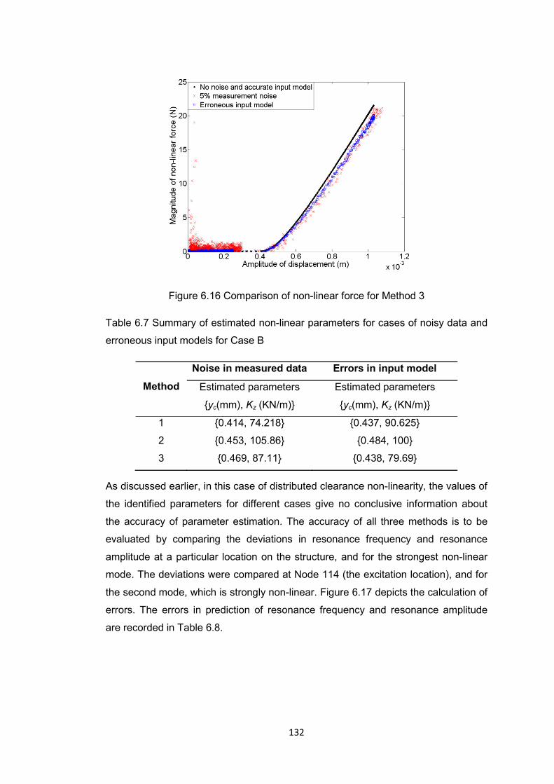
132
Figure 6.16 Comparison of non-linear force for Method 3
Table 6.7 Summary of estimated non-linear parameters for cases of noisy data and
erroneous input models for Case B
Method
Noise in measured data Errors in input model
Estimated parameters
{yc(mm), Kz (KN/m)}
Estimated parameters
{yc(mm), Kz (KN/m)}
1 {0.414, 74.218} {0.437, 90.625}
2 {0.453, 105.86} {0.484, 100}
3 {0.469, 87.11} {0.438, 79.69}
As discussed earlier, in this case of distributed clearance non-linearity, the values of
the identified parameters for different cases give no conclusive information about
the accuracy of parameter estimation. The accuracy of all three methods is to be
evaluated by comparing the deviations in resonance frequency and resonance
amplitude at a particular location on the structure, and for the strongest non-linear
mode. The deviations were compared at Node 114 (the excitation location), and for
the second mode, which is strongly non-linear. Figure 6.17 depicts the calculation of
errors. The errors in prediction of resonance frequency and resonance amplitude
are recorded in Table 6.8.

133
Figure 6.17 Depiction of calculation of errors for Case B
Table 6.8 Summary of errors in resonant response and resonance frequency
Method No noise and accurate input models
Noise in displacement measurements
Errors in input models
εy (%) εω (%) εy (%) εω (%) εy (%) εω (%)
1 3.78 6.68 1.71 7.54 4.55 6.36
2 6.08 5.72 6.45 5.57 3.71 6.71
3 3.45 6.82 2.01 7.42 1.94 7.44
It is observed from Table 6.7 that there is no trend in the error propagation due to
either noisy measurements or erroneous input model. The error in the prediction of
response is consistently higher for Method 2. It is also observed that the resonance
frequency is predicted less accurately than the resonance amplitude for this case.
The average value of errors in resonance frequency and resonance amplitude are
3.7% and 6.7% respectively, which are within acceptable limits for practical cases.
134
6.5 Discussion and concluding remarks
The three methods for non-linear parameter identification, presented earlier in the
thesis, have been compared on common ground using different criteria. Simulated
data obtained for the ‘1203 structure’, modelled using FEM with around two
thousand DOFs are used. Two cases with increasing complexity have been used for
the comparison. In the first case, an idealized grounded cubic stiffness non-linearity
is used, while in the second case, a more realistic clearance non-linearity over an
area of the structure is implemented. The identification of the non-linear parameters
has been carried out for both cases using the three methods to compare the
accuracy of parameter estimation. The conclusions of the comparison study are
listed below:
• It has been observed that, for all three methods, errors in the estimated
parameters are low when noise-free data along with an accurate input model of
the underlying linear structure are used. The effects of measurement noise and
erroneous input models are similar, to increase the error in parameter
estimation. It has been observed that the error increases by 5-9% depending on
the method.
• For all cases considered in this exercise, errors in the estimation of parameters
using Method 2 are found to be higher than when using the other two methods.
Method 1 has been found to identify the non-linear parameters accurately, even
with an erroneous FE model. It should be noted though; that the amount of
error in the underlying FE model, for which the method is tested, is very low.
This can only be achieved after successfully updating the FE model.
• It has been observed that Methods 1 and 3 possess the ability to locate the
non-linearity in the structure. Method 2 fails to locate the non-linearity, if the
location is unknown beforehand. This can sometimes put limitations on the use
of the method. On the positive side, Method 2 has successfully quantified the
level of non-linearity in each mode within the measured frequency range. This
information is useful at the later stage of parameter identification, for selecting
frequency lines to form the optimization problem.
• The computation times taken by the three methods are an order of magnitude
apart. Method 2 is the fastest of the three taking 2-orders of magnitude less
time than Method 1. Method 1 involves the inversion of a matrix of the size of
the number of un-measured DOFs, at each frequency line. For practical
structures where only few percent of the total number of DOFs are measured,
the matrix may become very large, making the computation inefficient. Method

135
3 consumes slightly more computation time than Method 2, but the order of
magnitude is comparable. For Method 3, the computation time is directly
proportional to the number of measured DOFs. Thus, the time can be reduced
by using fewer measurements.
• It has been noted that the deviation in the predicted response, as a result of
errors in non-linear parameters, is a function of the sensitivity of the structure to
those errors. For a less sensitive or a more robust structure, large errors in non-
linear parameters will probably yield a small deviation in the predicted
response. Thus, the errors in the parameter estimation should be viewed
keeping in perspective the robustness of the structure. Methods for calculating
the sensitivity and robustness of forced response for non-linear structures are
proposed in [118].
Based on the importance of different criteria for an engineer in his day to day
applications, a weighing factor can be assigned for each criterion. For example,
since having clean data and accurate input models may be a rare event in practice,
it can be given less weighing factor as against the performance of the methods with
noisy data and inaccurate input models. This approach of assigning the weighing
factor for each comparison criteria is subjective, and depends on what user wants
from the identification method.
A similar weighed evaluation is performed for the three methods to illustrate
the process. Table 6.9 shows a summary of the performance of the methods
quantified based on different evaluation criteria, weighing factor used for each
criterion, and the total score for each method. Every method is scored on a scale of
0-3 for each criterion. With the weighing factors assigned in the current study, the
FRF based method (Method 3) comes on top, providing the right mix of accuracy
and computational efficiency. The method uses all raw inputs directly obtainable
from vibration measurements. This eliminates the need of sophisticated tools like
FEA and modal analysis at the stage of parameter identification.

136
Table 6.9 Quantitative comparison of the three methods
Criteria Weighing
factor
Method
Spatial method (Method 1)
Improved hybrid modal technique
(Method 2)
FRF based method
(Method 3)
Performance with clean data and
accurate input models 0.05 3 2 3
Performance with clean data and erroneous input
models 0.25 3 2 3
Performance with noisy data and
accurate input models 0.25 3 2 3
Computation time 0.1 1 3 2
Ability to locate non-linearity 0.1 3 1 3
Ability to quantify non-linear modes 0.2 1 3 1
Ability to extract non-linear force explicitly 0.05 3 1 3
Total Score 2.4 2.15 2.5

137
Chapter 7
Experimental investigation of non-linearities in MACE structure This chapter presents an experimental investigation of non-linearities in a complex
mechanical structure. A sub-assembly of the so-called MACE structure is studied in
detail. Different non-linearity detection techniques are used to detect the presence
of non-linearity. The location and the type of non-linearity are identified using the
non-linearity characterization techniques presented in the earlier chapters. Both
parametric and non-parametric models are fitted into experimental data to describe
the non-linear behaviour of the sub-assembly. The models are then used to predict
the system response at different excitation levels.
7.1 Introduction
Different strategies for non-linear system identification have been proposed and
compared in the earlier chapters of this thesis. The illustration of the methods and
their comparison has been performed on simulated data. It has been mentioned in
Chapter 6 that validating the proposed methods with experimental data on a realistic
structure poses some additional challenges. This chapter attempts to tackle such
challenges using experimentally measured vibration data. The main aim of this
study is to improve the understanding of real-life non-linear structures and to gauge
the scope and applicability of the proposed non-linear system identification
strategies in such cases.
7.1.1 Choice of the structure
There are attempts in the literature to identify the non-linearities from vibration data
measured on representative structures [3, 26, 101, 119]. The structures used in
these exercises were intentionally designed to exhibit pure forms of non-linearities,
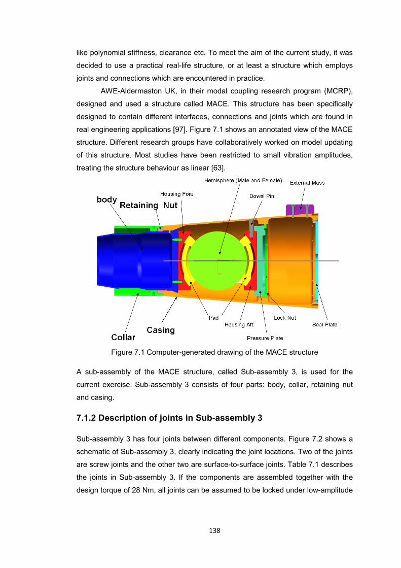
138
like polynomial stiffness, clearance etc. To meet the aim of the current study, it was
decided to use a practical real-life structure, or at least a structure which employs
joints and connections which are encountered in practice.
AWE-Aldermaston UK, in their modal coupling research program (MCRP),
designed and used a structure called MACE. This structure has been specifically
designed to contain different interfaces, connections and joints which are found in
real engineering applications [97]. Figure 7.1 shows an annotated view of the MACE
structure. Different research groups have collaboratively worked on model updating
of this structure. Most studies have been restricted to small vibration amplitudes,
treating the structure behaviour as linear [63].
Figure 7.1 Computer-generated drawing of the MACE structure
A sub-assembly of the MACE structure, called Sub-assembly 3, is used for the
current exercise. Sub-assembly 3 consists of four parts: body, collar, retaining nut
and casing.
7.1.2 Description of joints in Sub-assembly 3
Sub-assembly 3 has four joints between different components. Figure 7.2 shows a
schematic of Sub-assembly 3, clearly indicating the joint locations. Two of the joints
are screw joints and the other two are surface-to-surface joints. Table 7.1 describes
the joints in Sub-assembly 3. If the components are assembled together with the
design torque of 28 Nm, all joints can be assumed to be locked under low-amplitude
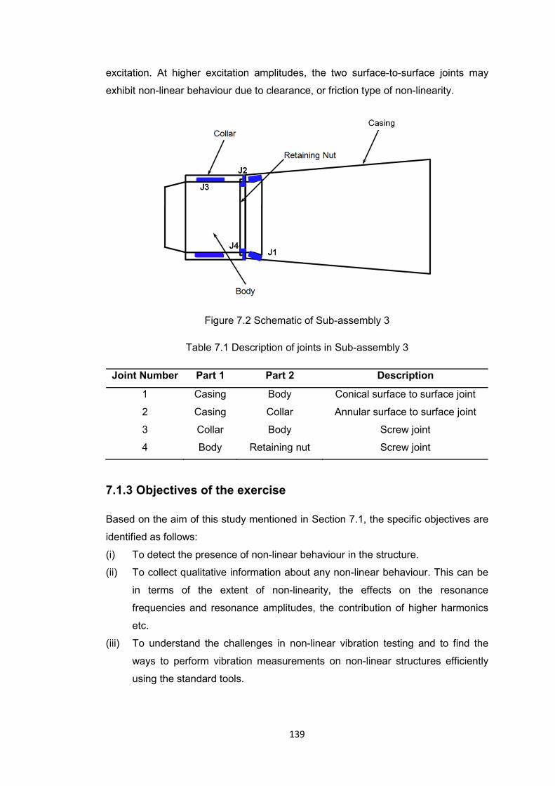
139
excitation. At higher excitation amplitudes, the two surface-to-surface joints may
exhibit non-linear behaviour due to clearance, or friction type of non-linearity.
Figure 7.2 Schematic of Sub-assembly 3
Table 7.1 Description of joints in Sub-assembly 3
Joint Number Part 1 Part 2 Description
1 Casing Body Conical surface to surface joint
2 Casing Collar Annular surface to surface joint
3 Collar Body Screw joint
4 Body Retaining nut Screw joint
7.1.3 Objectives of the exercise
Based on the aim of this study mentioned in Section 7.1, the specific objectives are
identified as follows:
(i) To detect the presence of non-linear behaviour in the structure.
(ii) To collect qualitative information about any non-linear behaviour. This can be
in terms of the extent of non-linearity, the effects on the resonance
frequencies and resonance amplitudes, the contribution of higher harmonics
etc.
(iii) To understand the challenges in non-linear vibration testing and to find the
ways to perform vibration measurements on non-linear structures efficiently
using the standard tools.

140
(iv) To attempt to locate the non-linearity, to extract the non-linear restoring force,
and to estimate the non-linear parameters using the proposed methods.
7.2 Validation of the FE models
To obtain a numerical model of the underlying linear structure, the components
were modelled using the FEM in ANSYS. The FE models of the three components,
the casing, the collar, and the body, were meshed using 3-D, 10-noded tetrahedral
elements (SOLID 187) with 3 DOFs per node. The retaining nut was not modelled
separately in this analysis, as it has insignificant mass compared to the other
components, and it would not add any significant stiffness to the system [63]. The
mesh size for the individual components was decided after checking the
convergence. Figure 7.3 shows a picture of three component meshes. The details of
material properties used for the components and the mesh sizing are given in
Appendix D.
Figure 7.3 FE models of the individual components
Modal properties for the individual components, in free-free condition, were obtained
by performing modal analysis on the FE models. The components were also tested
experimentally to find the modal properties using experimental modal analysis
(EMA). The global-M method, available in MODENT-2006 [117], was used for the
EMA. Because of axial symmetry of the components, double modes were obtained
at each natural frequency. Only one mode from the pair was used for the
comparison. The frequency range was restricted to 0-1000 Hz for the comparison.
Table 7.2 shows the results of the correlation between the FE models and the EMA.

141
Table 7.2 Correlation of modal properties for individual components
Component Mode Natural frequency (Hz) Discrepancy
(%) MAC
FEA EMA
Casing 1 584.8 585.7 0.15 0.98
2 712.1 706.9 0.74 0.97
3 1327.5 1328.4 0.07 0.99
Collar 1 515.4 513.1 0.45 0.96
2 854.3 826.7 3.33 0.92
3 1285.9 1301.0 1.16 0.87
Body 1 538.9 537.3 0.3 0.84
2 1197.5 1174.2 1.9 0.80
It is observed from Table 7.2 that the maximum discrepancy in the prediction of
natural frequencies using the FE models is around 3%. The minimum value of
modal assurance criteria (MAC) is 0.8. The low MAC value for some modes can be
attributed to the presence of double modes due to symmetric nature of the structure.
While identifying the modes via modal analysis, only one mode at a frequency was
identified. The correlation shows that the FE models of the individual components
are accurate enough for dynamic response predictions.
After obtaining the accurate FE models for the individual components, the
components were assembled together in ANSYS. In an ideal condition, all joints are
locked with no relative motion between the components. This condition was
simulated by using the option of bonded-contact, available in the ANSYS software.
The modal properties of the assembly were obtained by performing modal analysis
on the assembled FE model. Figure 7.4 shows the first twelve modes obtained via
FEA of the assembly.
To perform EMA on the assembled structure, the structure was suspended
freely using elastic cords. The FRFs were calculated by measuring the response at
one location and exciting the structure at several locations using an instrumented
hammer. The FRFs acquired with the excitation location on one side of the joints
and the response location on the other side, were found to be noisy. Because of the
poor transmissibility of force across the joints, all measurement locations were
selected from the Casing-side of the joints. This put a limitation on the number of
observable modes through the EMA. The modes which are local modes of the body
could not be identified. The modal properties were extracted using the multi-FRF
global-M method. Figure 7.5a shows the direct FRF plot along with the phase for the

142
assembled structure to give an idea regarding the quality of measurements. The
overlaid FRF measurements obtained via hammer testing are shown in Figure 7.5b.
Figure 7.4 Mode shapes of the assembled structure via FEA
Figure 7.5a Point FRF plot for the assembled structure (hammer test)

143
Figure 7.5b Overlaid FRFs for the EMA on the assembled structure
The modal properties of the assembled structure, extracted using the FEA and the
EMA, are compared in Table 7.3. It is observed that the difference in natural
frequencies is much higher than the difference observed in the correlation of
individual components. The maximum difference is around 15% for Mode 7. The
MAC values for the correlated modes are also lower when compared to the results
with the individual components. The high discrepancy suggests that the assumption
of locked joints used in the FE model may not be valid.
Table 7.3 Comparison of the modal properties of the assembled structure
Mode Natural frequency (Hz) Discrepancy
(%) MAC
FEA EMA
1 610.6 607.5 0.51 0.89
2 976.6 1002.5 2.58 0.67
3 1231.3 1110.4 10.89 0.75
4 1278.0 1211.3 5.51 0.69
5 1306.9 - - -
6 1361.8 - - -
7 1486.7 1292.4 15.03 0.59
8 1504.1 - - -
9 1578.6 - - -
10 1593.2 - - -
11 1615.5 - - -
12 1725.2 1715.0 0.59 0.93

144
The results can further be improved via model updating, or by using some interface
elements at the joint locations. The interface elements can be linear as implemented
in [63]. If the structure happens to be non-linear, the use of linear interface elements
will result in an equivalent linear model of the assembly at a particular excitation
level.
7.3 Detection of non-linear behaviour
Inherently, all assembled structures are non-linear to some extent. If the nominal
operating conditions are such that the structure does not exhibit any non-linear
behaviour, it is usually safe to use an equivalent linear model of the structure for
response predictions. It is therefore necessary to check if the structure is behaving
non-linearly in the operating range of excitations.
For linear vibration testing, impulse and random excitations are popular,
because they are less time consuming. For non-linear systems, the use of impulse
or random excitation tends to linearize the system about the operating point. On the
other hand, stepped-sine excitation, though time-consuming, is recommended for
non-linear systems [2, 120]. Most of the methods for non-linearity detection do not
make use of the mode shapes of the system. Thus, responses at only a few
locations are sufficient for non-linearity detection. In the current study, the
responses at the excitation location under different excitation levels are used to
detect non-linear behaviour.
7.3.1 Problem of force-drop near resonance
It has been stated in the literature [6, 7] that, with a constant supply of input current
to the exciter, the input force may vary with the excitation frequency. A drop in the
input force is usually observed when the excitation frequency is close to any of the
system’s resonance frequencies. For linear systems, since the ratio of response
over force is of primary interest, the force-drop phenomena can be overlooked. On
the other hand, for non-linear systems, if the input force is not kept constant, the
non-linearities are not exhibited properly. This may lead to erroneous system
identification. Figure 7.6 shows the force-drop phenomena, which was observed for
the MACE structure sub-assembly.

145
Figure 7.6 Force drop near resonance for the MACE sub-assembly
The direct FRF of the sub-assembly, around the first resonance, was measured at
different excitation levels with step-sine tests without force control. Figure 7.7 shows
the overlaid FRFs at different excitation levels. It can be seen from Figure 7.7 that
the FRFs at different excitation levels do not overlay perfectly, indicating the
presence of non-linearity. Thus, the non-linearity can be detected at a very early
stage, even without maintaining a constant value of the input force. But to
characterize the non-linearity type and to identify the non-linear parameters, the
step-sine tests with force control are required [2, 6, 7].
Figure 7.7 Overlaid FRFs at different excitation levels without force-control
The control algorithm used in the current research, to keep the input force constant,
is an iterative algorithm using the Newton Raphson method [101, 107]. Figure 7.8
shows the flowchart for the algorithm used. An in-house control system [101],

146
developed in the Lab-view software which implements this algorithm, was used to
carry out the force-controlled step-sine tests on the MACE sub-assembly.
Figure 7.8 Flow chart for the force-control algorithm

147
7.3.2 Non-linearity detection with constant-force step-sine tests
The control algorithm discussed in Section 7.3.1 was used to perfom constant-force
step sine tests on the MACE sub-assebmly. Figure 7.9 shows the experimental set-
up used for the experiment.
Figure 7.9 Experimental setup for non-linear step-sine testing
Since during the initial hammer testing it was observed that the first mode of
the sub-assembly was the most dominant mode, the detection, characterization and
parameter estimation of non-linearities were performed using the response around
this mode.
For the detection of non-linear behaviour, the response at the excitation
location was measured at different levels of excitation. Figure 7.10 shows the
overlaid FRFs at different excitation levels. It can be seen that the value of
accelerance drops continuously with increase in the force level. This suggests a
non-linear behaviour with energy dissipation. The resonance frequency is observed
to be reducing slightly with the increasing force level.

148
Figure 7.10 Overlaid accelerance at different excitation levels with force-control
The Nyquist plots for the same FRFs are overlaid in Figure 7.11. It can be observed
from Figure 7.11 that as the excitation amplitude increases, the Nyquist plots
become more elliptical. The presence of double modes, as discussed in Section 7.2
can be observed from the Nyquist plots in Figure 7.11.
Figure 7.11 Nyquist plots for accelerance at different excitation levels
The presence of higher harmonics in response is also an indicator of non-linear
behaviour of a system. In conventional vibration tests, spectral analysers calculate
FRFs by considering the fundamental harmonics only in the time-domain response.

149
To capture higher harmonics during the tests, raw time signals of the response were
acquired, and Fourier analysis was performed on the signals externally.
Figure 7.12 shows the contribution of the higher harmonics in the signal
captured at the resonance frequency for the excitation force of 10N. The presence
of higher harmonics is clearly visible from the figure. Figure 7.13 presents a bar
chart showing the amplitudes of the second and third harmonic components, at the
resonance frequency, for different values of excitation force. The amplitudes are
normalized to the fundamental harmonic component at each force level. From
Figure 7.13, it can be seen that, at higher excitation levels, the contribution of the
2nd and the 3rd harmonic components in the signal is significant, reaching to almost
20% of the fundamental harmonics at 10N excitation force. The higher contribution
of 2nd harmonic component may suggest a symmetric nature of non-linearity.
Figure 7.12 Presence of higher-harmonics in the response at 10N force level
After checking the system with different non-linearity detection techniques, it is
concluded that the sub-assembly behaves non-linearity at higher excitation
amplitudes.

150
Figure 7.13 Contribution of the higher harmonics at different excitation levels
7.4 Characterization of the non-linearity
Once it is verified that the MACE sub-assembly behaves non-linearly at high
excitation levels, the next stage is to find the location of non-linearity and to identify
the probable type of non-linearity. These tasks traditionally come under the realm of
non-linearity characterization.
At this stage of non-linear system identification, an accurate set of response
measurements at several locations distributed over the structure are required.
Because of the poor transmissibility of force through the connection area, as
discussed in Section 7.2, the measurement locations were distributed uniformly on
the casing-side of the joints. Figure 7.14 shows a schematic of the MACE sub-
assembly, indicating the locations of measurements. Four locations along the
length, denoted by the numbers 1 to 4, and four locations along the circumference,
denoted by the letters A to D, were selected for measurements. Thus, a total of 16
measurement locations were used in the analysis.
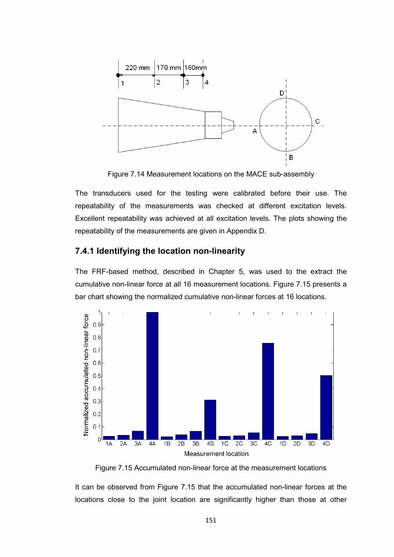
151
Figure 7.14 Measurement locations on the MACE sub-assembly
The transducers used for the testing were calibrated before their use. The
repeatability of the measurements was checked at different excitation levels.
Excellent repeatability was achieved at all excitation levels. The plots showing the
repeatability of the measurements are given in Appendix D.
7.4.1 Identifying the location non-linearity
The FRF-based method, described in Chapter 5, was used to the extract the
cumulative non-linear force at all 16 measurement locations. Figure 7.15 presents a
bar chart showing the normalized cumulative non-linear forces at 16 locations.
Figure 7.15 Accumulated non-linear force at the measurement locations
It can be observed from Figure 7.15 that the accumulated non-linear forces at the
locations close to the joint location are significantly higher than those at other

152
locations. Thus, the location of non-linearity is identified to be within the vicinity of
the joint.
7.4.2 Identifying the type of non-linearity
Before going to the last stage of actually estimating the non-linear parameters, it is
important to gain some knowledge about non-linear behaviour trend, and the
possible mathematical models which can be fitted into the observed behaviour.
The analysis of the responses obtained at different excitation levels provided
initial trends in the non-linear behaviour. The variations in the resonance amplitude
and in resonance frequency for the first mode of the sub-assembly were studied.
Figure 7.16 shows the variation of the resonance amplitude with the excitation level.
Figure 7.16 Variation of the resonance amplitude for the first mode
It is seen from Figure 7.16 that the resonance amplitude does not increase linearly
with the excitation force. The curve flattens beyond the force of 3N. This suggests
dissipative behaviour of non-linearity which might come from the frictional contacts
between the components.
Figure 7.17 shows the variation of resonance frequency with the excitation
force. It is observed that the resonance frequency drops with the excitation force,
suggesting a softening-stiffness behaviour of non-linearity.

153
Figure 7.17 Variation of the resonance frequency of the first mode
As explained in [6], the real and imaginary parts of inverse-accelerance can be used
to indicate the type of non-linearity. If the real part of an accelerance, plotted against
(frequency)2, deviates from a straight line, it indicates a stiffness type non-linearity.
Similarly, if the imaginary part of an accelerance plotted against frequency deviates
from a straight line, it indicates a damping type non-linearity.
The direct or point accelerance plots at different excitation levels were used
to identify whether the non-linearity is of stiffness-type or damping-type. Figure 7.18
shows the inverse-accelerance plot at the excitation force level of 5N. It can be seen
that both the real and imaginary parts deviate from a straight line, indicating the
presence of both stiffness and damping type of non-linearity.
Figure 7.18 Inverse FRF plots at excitation force level = 5N
Using the different techniques as above, a general idea about the non-linear
behaviour has been obtained. At this point, the reduction in peak amplitude of
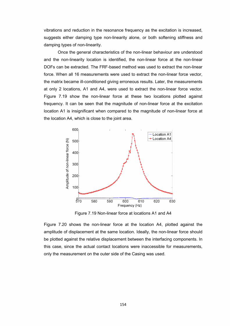
154
vibrations and reduction in the resonance frequency as the excitation is increased,
suggests either damping type non-linearity alone, or both softening stiffness and
damping types of non-linearity.
Once the general characteristics of the non-linear behaviour are understood
and the non-linearity location is identified, the non-linear force at the non-linear
DOFs can be extracted. The FRF-based method was used to extract the non-linear
force. When all 16 measurements were used to extract the non-linear force vector,
the matrix became ill-conditioned giving erroneous results. Later, the measurements
at only 2 locations, A1 and A4, were used to extract the non-linear force vector.
Figure 7.19 show the non-linear force at these two locations plotted against
frequency. It can be seen that the magnitude of non-linear force at the excitation
location A1 is insignificant when compared to the magnitude of non-linear force at
the location A4, which is close to the joint area.
Figure 7.19 Non-linear force at locations A1 and A4
Figure 7.20 shows the non-linear force at the location A4, plotted against the
amplitude of displacement at the same location. Ideally, the non-linear force should
be plotted against the relative displacement between the interfacing components. In
this case, since the actual contact locations were inaccessible for measurements,
only the measurement on the outer side of the Casing was used.

155
Figure 7.20 Non-linear force at A4 against displacement at A4
An interesting observation is made from Figure 7.20. Before and after the
resonance, the non-linear forces trace different paths, thus forming a loop. It can be
argued that the non-linear parameters as used in the conventional models,
corresponding to the friction and clearance non-linearity, change as the system
passes through a resonance.
The non-linear force at location A4 was extracted using two different
methods, the I-HMT method and the FRF-based method. It was found that the two
curves match closely. Figure 7.21 shows the comparison of non-linear force
extracted using the two methods.
Figure 7.21 Comparison of non-linear force extracted using different methods

156
To identify the type of non-linearity using the footprint library presented in
Chapter 3, the extracted non-linear force at A4 was compared with different
footprints in the library. The shape matching algorithm was used to find SSD values
for each non-linearity type. Figure 7.22 shows the comparison of the extracted non-
linear force with different non-linear footprints and the corresponding SSD values. It
is observed that the extracted non-linear force closely matches with (i) pure stick
type friction non-linearity and (ii) combined clearance and friction non-linearity, the
plots with a square border.
Figure 7.22 Comparison of the extracted non-linear force with footprint library
From the physics of the joints, the trend observed in the non-linear force,
and the quantitative comparison with the footprints from the library, it may be
concluded that the non-linearity present in the structure is of clearance and friction
type.
7.4.3 Estimation of non-linear parameters
This is the last stage in non-linear system identification in which the parameters of
the models which describe the non-linearities in the system are estimated. Since
measurements were distributed only on the casing, the relative displacements
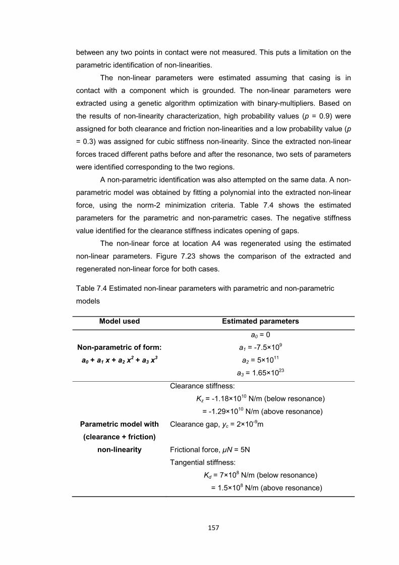
157
between any two points in contact were not measured. This puts a limitation on the
parametric identification of non-linearities.
The non-linear parameters were estimated assuming that casing is in
contact with a component which is grounded. The non-linear parameters were
extracted using a genetic algorithm optimization with binary-multipliers. Based on
the results of non-linearity characterization, high probability values (p = 0.9) were
assigned for both clearance and friction non-linearities and a low probability value (p
= 0.3) was assigned for cubic stiffness non-linearity. Since the extracted non-linear
forces traced different paths before and after the resonance, two sets of parameters
were identified corresponding to the two regions.
A non-parametric identification was also attempted on the same data. A non-
parametric model was obtained by fitting a polynomial into the extracted non-linear
force, using the norm-2 minimization criteria. Table 7.4 shows the estimated
parameters for the parametric and non-parametric cases. The negative stiffness
value identified for the clearance stiffness indicates opening of gaps.
The non-linear force at location A4 was regenerated using the estimated
non-linear parameters. Figure 7.23 shows the comparison of the extracted and
regenerated non-linear force for both cases.
Table 7.4 Estimated non-linear parameters with parametric and non-parametric
models
Model used Estimated parameters
Non-parametric of form: a0 + a1 x + a2 x2 + a3 x3
a0 = 0
a1 = -7.5×10⁹
a2 = 5×10¹¹
a3 = 1.65×10²³
Parametric model with (clearance + friction)
non-linearity
Clearance stiffness:
Kz = -1.18×10¹⁰ N/m (below resonance)
= -1.29×10¹⁰ N/m (above resonance)
Clearance gap, yc = 2×10⁻⁹m
Frictional force, µN = 5N
Tangential stiffness:
Kd = 7×10⁸ N/m (below resonance)
= 1.5×10⁸ N/m (above resonance)
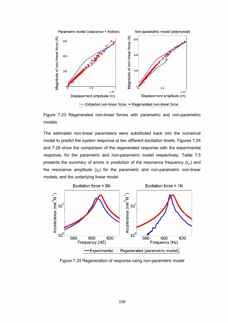
158
Figure 7.23 Regenerated non-linear forces with parametric and non-parametric
models
The estimated non-linear parameters were substituted back into the numerical
model to predict the system response at two different excitation levels. Figures 7.24
and 7.25 show the comparison of the regenerated response with the experimental
response, for the parametric and non-parametric model respectively. Table 7.5
presents the summary of errors in prediction of the resonance frequency (εω) and
the resonance amplitude (εy) for the parametric and non-parametric non-linear
models, and the underlying linear model
Figure 7.24 Regeneration of response using non-parametric model

159
Figure 7.25 Regeneration of response using parametric model
Table 7.5 Comparison of errors in the regenerated response
Model used Excitation force = 5N Excitation force = 1N
εω (%) εy (%) εω (%) εy (%)
Parametric 0.81 16.1 0.56 2.18
Non-parametric 0.96 12.3 1.02 40.7
Linear 0.48 76.6 0.23 3.13
From Table 7.5, it is observed that if the underlying linear model of the system is
used for the prediction, the discrepancy increase with the excitation force. This is
reasonable as with increase in the excitation force, the system moves into the non-
linear regime.
For non-linear models, the predictions at the excitation force of 5N, at which
the non-linear system identification was carried out, are fairly accurate. The
maximum error in the prediction of peak response is around 16%. When these
same models are used to predict the dynamic behaviour at the excitation force of
1N, out of the two models, the parametric model performs better. Still the shape of
plots for predicted and observed response at 1N are different. This may be because
the parametric model identified in the current study does not utilise the relative
displacements between the two parts in contact. Thus, the clearance and friction
models fitted are not parametric in true sense. It is necessary to investigate the
effect of approximating relative displacement by the absolute displacement at one of
the contributing DOF. This can be checked on a simple 3 DOF system, with non-
linearity acting between any two DOFs.

160
Since the regeneration capability of the models is checked at only two
discrete excitation levels, it cannot be concluded that the identified models are valid
over a wide range of operating conditions.
7.5 Concluding remarks
This chapter presents the results of an experimental investigation of non-linearities
in the MACE structure sub-assembly. It has been observed that when the accurate
FE models of the individual components are assembled together with the locked-
joints assumption, the predictions for the assembled structure are inaccurate. This
suggests some relative motion between different parts of the joints, which may
contribute towards the non-linear behaviour of the system.
The results of different non-linearity detection techniques have been
presented to conclude that the structure’s behaviour is significantly non-linear at
higher excitation levels. The measurements at different excitation levels were used
to characterize the non-linear behaviour. Softening-stiffness type behaviour along
with dissipating mechanism has been observed in the structure. It has been
observed that the detection of non-linear behaviour and approximate
characterization of non-linearity type can be successfully performed with very limited
measurement data.
The measurement data from the constant-force step-sine vibration tests,
performed at relatively high force amplitude, were used to extract the non-linear
force vector at the measured locations. The accumulated non-linear force plots were
used to locate the non-linearity. The locations close to the joint location have been
correctly identified as the non-linearity locations. The extracted non-linear force at
the non-linear location was compared with the curves from the footprint library for
type identification. The SSD values corresponding to the combined clearance and
friction non-linearity and pure-stick friction non-linearity were found to be the lowest.
This type identification is consistent with engineering judgement.
The results of both parametric and non-parametric identifications have been
presented. The identified models are found to be accurate at the excitation level at
which they were identified. The extrapolation capacity of the models and their
universality needs to be verified.

161
Chapter 8
Non-linear parameter identification for base-excited structures This chapter presents a method for non-linear system identification of base-excited
structures with controlled acceleration input. The proposed method works in three
stages to estimate the non-linear parameters in a system. The method is entirely
based on measured data with no need for an FE model. The proposed method is
illustrated on a pyramid-like structure using simulated data. The performance of the
method in the presence of measurement noise is also evaluated.
8.1 Introduction
The civil engineering structures like buildings, bridges, stadia and dams are often
designed to avoid the transmissibility of ground vibrations. For laboratory testing of
such structures, a scaled model of the structure is mounted on a shaker table, and it
is given acceleration input at the base to simulate operating conditions. Similar tests
are sometimes performed for military applications, spacecrafts and aircraft
structures, to evaluate their dynamic performance under base loading. In such
cases, the excitation forces do not act locally, but they are distributed throughout the
structure, depending on mass distribution in the structure.
The traditional non-linear parameter identification techniques described in
[28, 36-38], and the methods proposed in Chapters 4 and 5 of this thesis, require
force and response information at all excitation DOFs for their successful
implementation. For cases where the excitation comes from acceleration input,
these requirements can be met only if: (i) all DOFs are measured, and (ii) the mass
distribution in the structure is known a-priori. Thus, in practical cases it may not be
possible to use the available identification methods directly.
The chapter presents a three stage strategy for non-linear system
identification in case of base-excited structures.
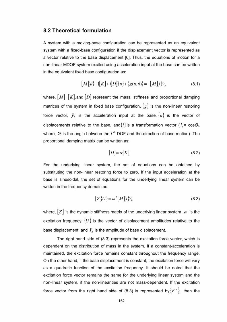
162
8.2 Theoretical formulation
A system with a moving-base configuration can be represented as an equivalent
system with a fixed-base configuration if the displacement vector is represented as
a vector relative to the base displacement [6]. Thus, the equations of motion for a
non-linear MDOF system excited using acceleration input at the base can be written
in the equivalent fixed base configuration as:
[ ]{ } [ ] [ ]( ){ } { } [ ]{ } bylMuuguDiKuM &&&&& −=+++ ),( (8.1)
where, [ ]M , [ ]K ,and [ ]D represent the mass, stiffness and proportional damping
matrices of the system in fixed base configuration, { }g is the non-linear restoring
force vector, by&& is the acceleration input at the base, { }u is the vector of
displacements relative to the base, and{ }l is a transformation vector ( il = cosØi,
where, Øi is the angle between the i th DOF and the direction of base motion). The
proportional damping matrix can be written as:
[ ] [ ]KD α= (8.2)
For the underlying linear system, the set of equations can be obtained by
substituting the non-linear restoring force to zero. If the input acceleration at the
base is sinusoidal, the set of equations for the underlying linear system can be
written in the frequency domain as:
[ ]{ } [ ]{ } bYlMUZ 2ω= (8.3)
where, [ ]Z is the dynamic stiffness matrix of the underlying linear system ,ω is the
excitation frequency, { }U is the vector of displacement amplitudes relative to the
base displacement, and bY is the amplitude of base displacement.
The right hand side of (8.3) represents the excitation force vector, which is
dependent on the distribution of mass in the system. If a constant-acceleration is
maintained, the excitation force remains constant throughout the frequency range.
On the other hand, if the base displacement is constant, the excitation force will vary
as a quadratic function of the excitation frequency. It should be noted that the
excitation force vector remains the same for the underlying linear system and the
non-linear system, if the non-linearities are not mass-dependent. If the excitation
force vector from the right hand side of (8.3) is represented by { }dF , then the

163
equations for the linear system can be written in terms of the FRF matrix of the
system as
{ } [ ]{ }dFU α= (8.4)
In practical cases, not all DOFs of the system can be measured. To deal with this,
(8.4) is partitioned into the measured and un-measured DOFs:
⎭⎬⎫
⎩⎨⎧⎥⎦
⎤⎢⎣
⎡=
⎭⎬⎫
⎩⎨⎧
du
dm
uuum
mumm
u
m
FF
UU
αααα
(8.5)
Considering only the measured responses from (8.5), we can write:
{ } [ ]{ } [ ]{ }dumu
dmmmm FFU αα += (8.6)
Multiplying (8.6) by [ ] 1−mmα , we get a pseudo excitation force vector at the measured
DOFs as:
{ } { } [ ] [ ]{ }dumumm
dm
d FFP αα 1−+= (8.7)
This vector can be considered as the projection of the excitation force vector of the
entire system onto the measured DOFs. It is possible to extract this vector solely
from the measured data as:
{ } [ ] { }mmmd UP 1−= α (8.8)
Now, for a non-linear system, the equation for harmonic amplitude can be written
as:
{ } [ ]{ } [ ]{ }dFGU αα =+~ (8.9)
where, { }U~ represents the non-linear response vector relative to the base.
Partitioning (8.9) into measured and un-measured DOFs, the non-linear force vector
at the measured DOFs can be extracted as:
{ } { } [ ] [ ]{ }( ) [ ] [ ]{ }( ) [ ] { }mmmumummd
umummd
mm UGFFG ~111 −−− −−+= ααααα (8.10)
If non-linearities are confined to the measured zone,{ }uG can be set to zero and
(8.10) becomes:
164
{ } { } [ ] [ ]{ }( ) [ ] { }mmm
P
dumumm
dmm UFFG
d
~11 −− −+= ααα4444 34444 21 (8.11)
As the pseudo excitation force vector remains same for linear and non-linear
systems if the non-linearities do not cause mass matrix variation, (8.10) can be
written as
{ } { } [ ] { }mmmd
m UPG ~1−−= α (8.12)
Once the non-linear force vector corresponding to the measured DOFs is extracted
using (8.12), the non-linearity location can be identified by plotting the cumulative
non-linear force. The non-linear force at the non-linear DOF can then be used to
extract the non-linear parameters using a genetic algorithm optimization.
8.3 Implementation of the method
The proposed method is applied in 3 stages: at the first stage, the pseudo excitation
force vector at the measured DOFs is extracted using (8.8). To do this, beforehand
the FRF matrix of the underlying linear structure is obtained via modal analysis of
the structure in fixed base configuration at low excitation levels. The vector of
relative displacements for the underlying linear structure is then obtained by
performing slip-table tests with low acceleration input.
The second stage consists of extracting the non-linear force vector at the
measured DOFs. First the relative non-linear displacement vector is measured by
subjecting the structure to high acceleration input at the base. The non-linear force
is then extracted using (8.12).
In the last stage, the non-linear force at the measured DOFs is used to
estimate the non-linear parameters via genetic algorithm optimization. Figure 8.1
shows the flowchart for the method.

165
Figure 8.1 Flowchart of the proposed method
8.4 Illustration of the method
The proposed method is illustrated on Validation structure-3; a pyramid-like
structure made of 4 beams and mounted on a rigid platform. The slip-table tests can
be simulated by giving the platform a constant acceleration input. Figure 8.2 shows
the schematic of the structure with measurement locations, non-linearity location,
and the node numbers. The detailed engineering drawing of the structure and the
properties of materials used are documented in Appendix B.
For the current simulation, the platform was given a constant acceleration in
X direction. A grounded cubic stiffness non-linearity, acting in X direction was
placed at one of the beams (Node 7). The non-linear coefficient β = 5×10¹² Nm-3,
was used for the simulation. To mimic the condition of incomplete measurements,
displacement responses in the X direction were measured at 5 nodes including the

166
non-linear DOF. A constant modal damping of 1% (η =0.01) was used in the
simulation.
Figure 8.2 Schematic of Validation structure-3
8.4.1 Stage 1: Extraction of pseudo excitation force vector (Pd)
To extract the pseudo excitation force, the FRF matrix, and the relative
displacement vector of the underlying linear structure are required. The FRF matrix
of the structure, [ ]mmα , corresponding to the measured DOFs, in the fixed-base
configuration, was obtained by performing modal analysis on the system matrices.
Figure 8.3 shows the overlaid FRFs. The displacement responses at the measured
DOFs were then obtained by giving a constant acceleration of 0.09 m/s2 to the
base. The low value of acceleration resulted in close-to-linear behaviour of the
structure. Thus, the relative displacement vector ( U ), of the underlying linear
structure, was calculated.
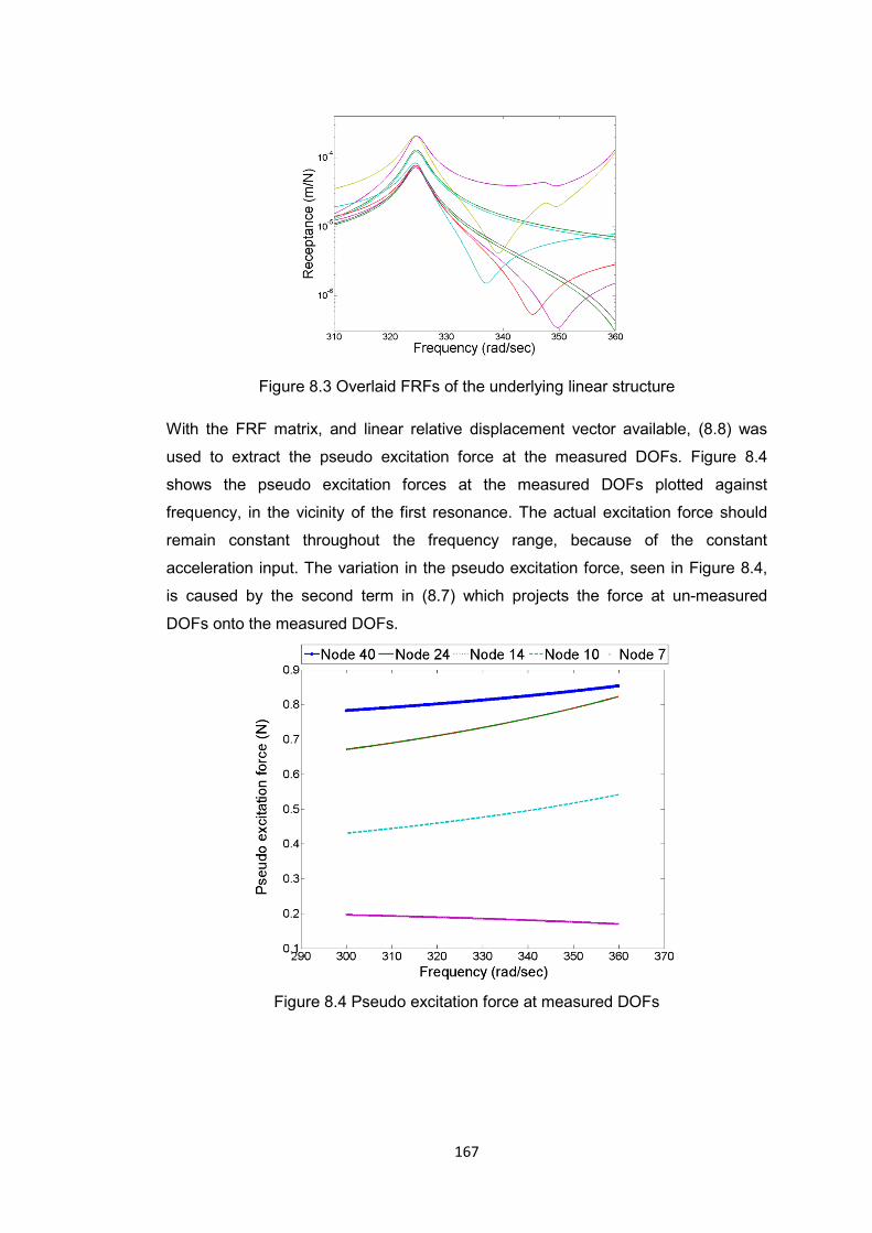
167
Figure 8.3 Overlaid FRFs of the underlying linear structure
With the FRF matrix, and linear relative displacement vector available, (8.8) was
used to extract the pseudo excitation force at the measured DOFs. Figure 8.4
shows the pseudo excitation forces at the measured DOFs plotted against
frequency, in the vicinity of the first resonance. The actual excitation force should
remain constant throughout the frequency range, because of the constant
acceleration input. The variation in the pseudo excitation force, seen in Figure 8.4,
is caused by the second term in (8.7) which projects the force at un-measured
DOFs onto the measured DOFs.
Figure 8.4 Pseudo excitation force at measured DOFs
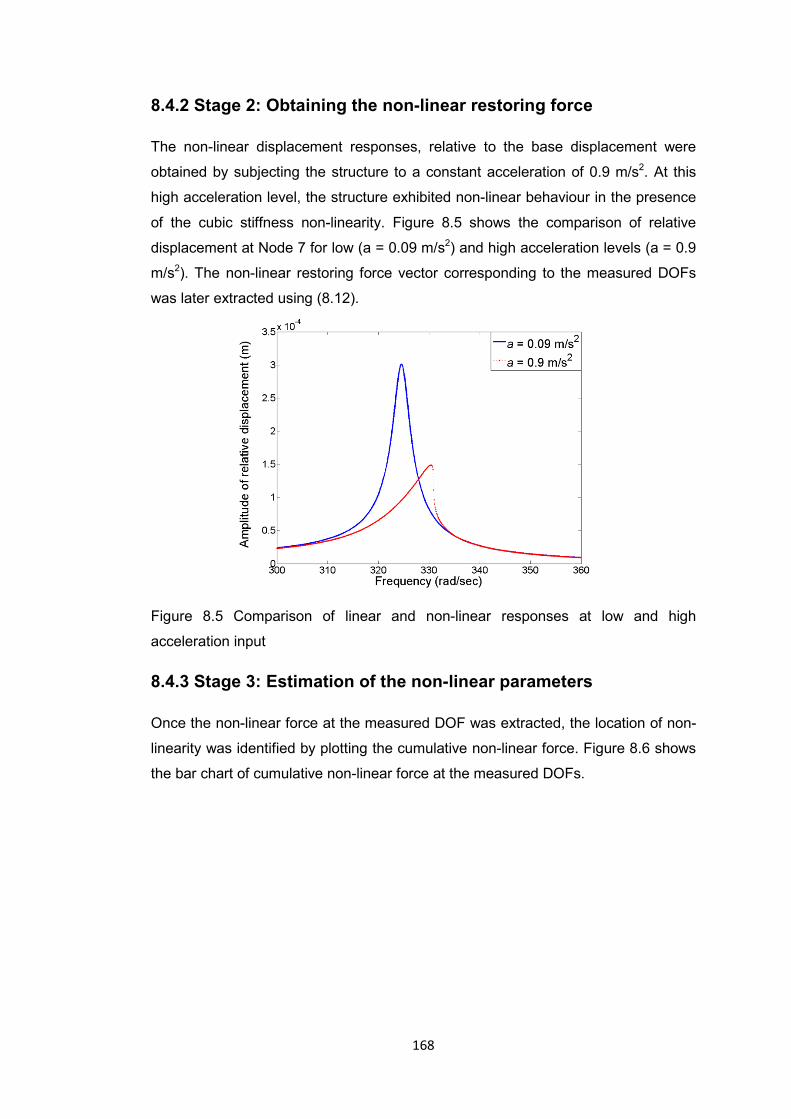
168
8.4.2 Stage 2: Obtaining the non-linear restoring force
The non-linear displacement responses, relative to the base displacement were
obtained by subjecting the structure to a constant acceleration of 0.9 m/s2. At this
high acceleration level, the structure exhibited non-linear behaviour in the presence
of the cubic stiffness non-linearity. Figure 8.5 shows the comparison of relative
displacement at Node 7 for low (a = 0.09 m/s2) and high acceleration levels (a = 0.9
m/s2). The non-linear restoring force vector corresponding to the measured DOFs
was later extracted using (8.12).
Figure 8.5 Comparison of linear and non-linear responses at low and high
acceleration input
8.4.3 Stage 3: Estimation of the non-linear parameters
Once the non-linear force at the measured DOF was extracted, the location of non-
linearity was identified by plotting the cumulative non-linear force. Figure 8.6 shows
the bar chart of cumulative non-linear force at the measured DOFs.

169
Figure 8.6 Identification of non-linearity location
It can be seen from Figure 8.6 that the cumulative non-linear force is maximum at
Node 7, and its magnitude is significantly higher than the magnitude of forces at
other nodes. This correctly identifies the location of non-linearity. Figure 8.7 shows
the plot of non-linear restoring force at the identified non-linear DOF.
Figure 8.7 Non-linear force at the non-linear DOF
The non-linear force at the non-linear DOF was then used to extract the non-linear
parameters using the genetic algorithms. The initial range for the parameter in the
GA was kept from 0 to 5×14 Nm-3. The range was narrowed in subsequent
civilizations to gain accuracy. The value of identified parameter and the
corresponding error is recorded in Table 8.1.

170
8.4.4 Performance in the presence of experimental noise
Since the method relies completely on measured data, it is important to check the
sensitivity of the method to measurement noise. There are three quantities which
are obtained from experimental measurements: the FRF matrix, the response at low
excitation level, and the response at high excitation level. Each of these can act as
a source of measurement noise. Thus, four different cases were considered in order
to analyse the effects of noise in each measured quantity independently, and the
combined effect noise in all three.
In the first case, only the FRF matrix, [ ]mmα , was polluted with artificial noise
of 3% using equation (6.1) from Chapter 6. In the second and the third case, the
response vectors,{ }mU and { }mU~ were polluted with 3% noise respectively, using
(4.15). Table 4.1 summarizes the results for all these cases.
Table 8.1 Estimated parameters with and without noise
Case Noise
level (%) Estimated value of
β ×1012 (Nm-3) Error in
estimation (%)
No-noise 0 5.06 1.2
Noise in the FRFs 3 5.09 1.8
Noise in linear responses 3 5.84 16.8
Noise in non-linear
responses
3 6.37 27.4
Noise in all three 3 7.10 42
It can be seen from Table 8.1 that the non-linear parameter is identified accurately
with noise-free measurement data. For the cases with noise, the error is highest
when all three measured data contain noise, which was expected. The effect of
noise in FRF matrix is observed to be the least. Overall, it is observed that the
method is sensitive to measurement noise, and the error of the order of 40%, which
is reported in this study, may not be acceptable in many cases.
8.5 Concluding remarks
A method for the parametric identification of non-linearities for base-excited
structures has been proposed. The formulation of the method can be used for any
direction of base motion. The method is applicable in case of constant base

171
displacement or constant base acceleration configuration. The method uses only
raw measurement data, eliminating the need for the FE model of a structure.
The method has been illustrated on a pyramid-like structure with simulated
data. The method was found to be accurate in the absence of experimental noise.
There are three different sources of experimental noise in this method. In the case
where noise from all three sources is considered, the method estimated parameters
with around 40% error, which may be un-acceptable in many cases. Thus, the
method demands clean measurement data to identify the non-linear parameters
accurately.
Though the method is presented for base-excited structures, it is generic,
and can be extended for any case in which the excitation force is not measured.
The extension of this method to the output-only non-linear tests can be beneficial.

172
Chapter 9
Conclusions and future work This chapter concludes the thesis by presenting a summary of the research
findings, contributions by the author, details of published research papers from this
work, and finally the author’s view, on the scope of further research in this area.
9.1 Conclusions of the research work
Non-linear structural dynamics is an important research topic, relevant to different
industries. It encompasses various sub-areas like non-linear system identification,
stability studies for non-linear systems and the prediction of dynamic response for a
non-linear system. The work in this thesis is restricted to parametric identification of
non-linear systems in the frequency-domain. Different strategies for non-linear
system identification are proposed, and they are illustrated with the use of simulated
non-linear response data. During the research, the focus is always kept on the
practicality of the proposed strategies, and their integration with the established
tools like finite element analysis, modal testing and modal analysis. The detailed
conclusions on different topics are presented below.
9.1.1 Type characterization using footprints
Identifying the type of non-linearity is an important step in the parametric
identification of non-linear systems. Once the type of non-linearity is identified
correctly, a mathematical function can be chosen to fit the identified non-linearity. It
has been previously reported in the literature that the shape of non-linear restoring
force in a system is unique to the type of non-linearity. Taking this observation
further, a library of non-linear force footprints for different non-linearities, plotted in
different formats like Bode plots and Nyquist plots, has been generated. This library
can be used as a look-up chart for subjective identification of non-linearity type.
173
It has been observed that, if the non-linear force for a system is plotted
against the relative displacement amplitude at the non-linear DOFs, the shape of
the curve is independent of the underlying linear system. Thus, the footprint library
which is generated using a 2 DOF system can be used for identifying non-linearity
types for any practical non-linear system.
The type of non-linearity in a system can be identified by visual comparison
of the extracted non-linear force with the forces from the footprint library. To avoid
subjectivity in the visual comparison, a shape-matching algorithm has been
proposed for numerical comparison of non-linear forces.
For individual non-linearities, the algorithm proved to be accurate, correctly
identifying the non-linearity type. For the case of combined non-linearities, it has
been observed that the shape of non-linear force plot is dependent on the
contribution of each non-linearity type in the non-linear force. As this contribution
may vary from case to case, the correct identification of non-linearity type was found
difficult to achieve with the current footprint library. If the library is extended to
include footprints of combined non-linearities with unequal contributions, it may be
possible to identify the type of non-linearity, and even the contribution of each non-
linearity type.
9.1.2 Genetic algorithm optimization
In the current research, the last stage in the parametric identification, that of
estimating the non-linear parameters, has been formulated as an optimization
problem. The optimization problem, with non-linear parameters as design variables,
has been solved via a genetic algorithm. The method has been found to
successfully estimate the non-linear parameters, even if the non-linearity type is not
known a-priori. This feature is important in practical cases where the type of non-
linearity may not be identified.
A novel concept of ‘binary-multipliers’ has been proposed to efficiently
estimate the non-linear parameters if a user has some idea about the type of non-
linearity in a system. A significant improvement in the computational efficiency has
been achieved with the use of the binary multipliers.
9.1.3 On the choice of the model for the underlying linear system
The basic formulation proposed in the thesis requires a numerical model of the
underlying linear system. Three methods, each using different form of model for the
underlying linear system, has been investigated and compared.

174
It has been observed that the FRF-based method, which uses a response
model of the underlying linear system, performs better in the weighted comparison
against the other two methods. This method uses data directly from vibration
measurements, thus eliminating the need for analysis tools like FEA and modal
analysis. On the downside, the use of raw measurement data makes the method
susceptible to random noise in measurements.
The spatial method which uses an updated FE model of the underlying linear
system has been found to be sensitive to errors in the FE model. Moreover, for
practical structures with large system matrices, the method becomes
computationally expensive. As it may be difficult to obtain an accurate FE model of
a complex structure, this method may have a limited use in practice.
The I-HMT method, which uses a modal model of the underlying linear
system, has been found to be less accurate than the other two methods, but the
fastest of all three. This method also possesses an important feature of quantifying
the level of non-linearity in each mode, thus enabling users to select the modes
which are to be considered in further non-linear analysis.
Since the basic methodology for all three methods assumes frequency-
independent non-linear parameters, the number of equations available to solve the
optimization problem is usually much higher than the number of design variables.
Thus, a few measurements are sufficient to identify the non-linear parameters. For
all three methods, it has been observed that if measurements at all non-linear DOFs
and excitation DOFs are available, the non-linear parameters can be estimated
accurately. Moreover, it has been observed that the effect of measurement noise
increases with the number of measurements used in the analysis. Thus, it may be
best to use only the minimum required number of measurements.
For a successful application of all three proposed methods, measurements
must be taken very close to the non-linearity locations. This may put limitations on
the use of these methods in the case when the non-linearities are at several un-
accessible locations.
9.1.4 Experimental investigation of non-linear behaviour
To understand the difficulties faced by an engineer when dealing with
experimentally measured vibration data on a real-life engineering structure, a study
was undertaken on the MACE structure sub-assembly, which employs different
joints. The structure was found to behave non-linearity under high excitation
amplitudes.

175
It has been observed that the methods available in the literature, and those
proposed in this thesis allow detection, and approximate type characterization of
non-linearities at early stage of analysis with only a few measurements. Since non-
linearities in real-life engineering structures may not behave as per their idealized
mathematical form, a universal non-linearity identification method may not be readily
applicable in such cases.
From the results of the experimental study conducted in this research, the
author would suggest that the methods proposed in this thesis, and those available
in the literature may be used at initial stages of the analysis to get an idea about the
non-linear behaviour of a structure. Later on, the non-linearities may be identified
within relevant frequency and excitation ranges based on the operating conditions.
A universal model of a non-linear system may be difficult to identify for practical
engineering systems. A non-parametric identification may prove easier in such
cases, but again the model obtained via non-parametric identification may not be
accurate over a wide frequency and amplitude ranges of the input excitation.
It has also been observed that the contribution of higher harmonics was
significant in the response captured near the resonance frequency of the structure.
Thus, it may be best to check the contribution of higher-order harmonics in the
response before employing non-linear identification methods which are based on
the first order describing functions.
9.1.5 Identification method for base-excited structures
In the tests, in which the excitation comes from an acceleration input at the base,
the excitation force is distributed over the entire structure, and is usually not
measured. Thus, the conventional non-linear system identification methods may not
be directly applicable in such cases. To overcome this difficulty, a three-stage
method for non-linear system identification has been proposed. The method works
for both, acceleration controlled and displacement controlled tests. The method has
been found to be applicable for any oblique excitation direction. Though the method
is presented for base-excited structures, the same formulation can be extended to
the case of output-only tests which are performed in an actual operating
environment.

176
9.3 Contributions and publications of the thesis
The summary of the author’s contribution to the research field is presented below:
• A novel idea of a footprint library containing non-linear force for different
individual and combined non-linearities.
• A shape-matching algorithm to numerically compare the extracted non-linear
force with the curves from the footprint library.
• A genetic algorithm based optimization methodology to estimate the non-linear
parameters from the non-linear force.
• A concept of binary multipliers to improve the computational efficiency of the
genetic algorithm by making use of partial information known to a user regarding
the type of non-linearity in the system.
• Validation and comparison of the proposed non-linear identification methods on a
MDOF representative engineering structure.
• The development of non-linear system identification method for base-excited
structures.
A part of the work presented in this thesis is published in the following conference
and journal articles:
(1) Gondhalekar A. C., Petrov E. P., Imregun M., “Identification of MDOF
nonlinear system using genetic algorithm optimization”, International modal
analysis conference (IMAC)- XXVII, Florida-2008.
(2) Gondhalekar A., C., Petrov E. P., Imregun M, “Parameters identification for
nonlinear dynamic systems via genetic algorithm optimization”, Journal of
computational and nonlinear dynamics, Vol-4(4), pp 1-9, 2009.
9.4 Suggestions for future work
The research presented in this thesis started with the aim of developing strategies
for parametric non-linear system identification, which can be used for practical
engineering structures. Still at the end of this research certain questions remain

177
unanswered. The research in the area of non-linear system identification can be
taken further in the direction of topics presented below:
• The formulation in the thesis uses the first-order describing functions to model
the non-linear elements. The experimental investigation on the MACE structure
showed a significant presence of higher order harmonics in the response near
the resonance frequency. It would highly valuable to extend the current methods
to use higher order describing functions and compare the accuracy with the
methods presented here.
• The footprint library presented in this thesis has footprints of combined non-
linearities, which are prepared based on an equal contribution assumption. In
practice, different non-linearities may not always contribute equally in the non-
linear force. This makes it difficult to identify the combined non-linearities with
the current footprint library. The idea of banded-footprints, which is mentioned in
Chapter 3, can be pursued further to create an extended footprint library with
different contributions of non-linearities.
• The methods presented in the thesis are applicable for structures with localized
non-linearities. Moreover, the response very close to the non-linearity location
must be measured for their successful application. It would be valuable to
propose methods which are applicable for structures with distributed non-
linearities.
• The quantification of non-linear behaviour is still an area of research. There
haven’t been many methods described in the literature to quantify the level of
non-linearity in a system. It would be a nice piece of research to propose certain
criteria to quantify the level of non-linearity in a structure.
• From practical point of view, non-linear system identification is only an
intermediate task, in the bigger aim of predicting the system response. Some
systems are more sensitive to the errors in non-linear parameters than others.
Thus, it is necessary to calculate the sensitivity of a system to errors in the non-
linear parameters, and evaluate the performance of any identification method by
keeping the sensitivity in perspective. A tool which integrates these two would
be worth researching.

178
References
1. Imregun M.. Special issue on non-linear structural dynamics. Mechanical Systems and Signal Processing 23[1], 5-7. 2009.
2. Tomlinson G.R. and Worden K.. Nonlinearity in structural dynamics- Detection, identification and modelling. 2000. Bristol, Institute of Physics Publishing.
3. Golinval J.C., Kerschen G., Lenaerts V., Thouverez F., and Argoul P.. European COST action F3: Identification of nonlinear systems. Activities and results. Proceedings of ISMA 2002 III, 1177-1182. 2002.
4. Petrov E. and Ewins D.J.. State-of-the-art dynamic analysis for nonlinear gas turbine structures. Journal of Aerospace Engineering, Proc.of the IMech E 218[G3], 199-211. 2004.
5. Goege D.. Fast identification and characterization of nonlinearities in experimental modal analysis of large aircraft. Journal of Aircraft 44[2], 399-409. 2007.
6. Ewins D.J.. Modal testing: Theory and practice. 1984. Research Studies Press.
7. Maia N.M.M. and Silva J.M.M.. Theoretical and experimental modal analysis. 1997. Taunton, Somerset, England, Research Studies Press Ltd.
8. Gelb A. and Vander Velde W.E.. Multiple-input describing functions and nonlinear system design. 1968. New York, McGraw-Hill book company.
9. Goge D., Sinapius M., Fullekrug U., and Link M.. Detection and description of non-linear phenomena in experimental modal analysis via linearity plots. International Journal of Non-linear Mechanics 40, 27-48. 2005.
10. Imregun M.. Survey of non-linear analysis tools for structural systems. The Shock and Vibration Digest 30[5], 363-369. 1998.
11. Kerschen G, Worden K., Vakasis A.F., and Golinval J.C.. Past present and future of nonlinear identification in structural dynamics. Mechanical Systems and Signal Processing 20, 505-592. 2006.
12. Vanhoenacker K., Schoukens J., Swevers J., and Vaes D.. Summary and comparing overview of techniques for the detection of nonlinear distortions. Proceedings of ISMA 2002 III, 1241-1256. 2002.
13. Natke H., Jaung J.N., and Gawronski W.. A brief review on the identification of non-linear mechanical systems. Proceedings of IMAC-VI , 1569-1574. 1988.
14. Nayfeh A.H. and Mook D.T.. Nonlinear oscillations. 1979. Virginia, USA, John Wiley & Sons, Inc.
15. Ewins D.J.(Editor). Dynamic testing agency handbook on guidelines to best practice: Modal testing V.3. 1996.
16. Sjoberg J., Zang Q., Ljung L., Benveniste A., Delyon B., Glorennec P., Hjalmarsson H., and Juditsky H.. Nonlinear blackbox modelling in system identification- A unified overview. Automatica 31[12], 1691-1724. 1995.
17. Sjoberg J., Zang Q., Ljung L., Benveniste A., Juditsky H., Delyon B., Glorennec P., and Hjalmarsson H.. Nonlinear blackbox modelling in system identification: The mathematical foundation. Automatica 31[12], 1725-1750. 1995.
18. Vanlanduit S., Guillaume P., Schoukens J., and Vanhoenacker K.. Detection and localization of nonlinearities using a scanning laser vibrometer. Proceedings of ISMA-25 1, 473-482. 2000.
19. Schoukens J., Pintelon R., Rolain Y., and Dobrowiecki T.. Frequency response function measurements in the presence of nonlinear distortions. Automatica 37[6], 939-946. 2001.
179
20. Ewins D.J. and He J.. A simple method of interpretation of the modal analysis of nonlinear systems. Proceedings of IMAC V , 626-634. 1987. London, England.
21. Mertens M., Auweraer H.V., Vanherck P., and Snoeys R.. The complex stiffness method to detect and identify non-linear dynamic behaviour of SDOF systems. Mechanical Systems and Signal Processing 3[1], 37-54. 1989.
22. Tomlinson G.R.. Developments in the use of the hilbert transform for detecting and quantifying non-linearity associated with frequency response functions. Mechanical Systems and Signal Processing 1, 151-171. 1987.
23. Wyckaert K.. Development and evaluation of detection and evaluation schemes for the nonlinear dynamical behaviour of mechanical structures. PhD Thesis . 1992. Department of Mechanical Engineering, Division PMA, Katholieke Universiteit Leuven.
24. Chong Y.H. and Imregun M.. Use of reciprocal modal vectors for nonlinearity detection. Archive of Applied Mechanics 70, 453-462. 2000.
25. Kim W.J. and Park Y.S.. Non-linearity identification and quantification using an inverse fourier transform. Mechanical Systems and Signal Processing 3, 239-255. 1993.
26. Elizalde H.. Non-linear modal analysis methods for engineering structures. PhD Thesis . 2004. London, Imperial College, London.
27. Al-Hadid M.A. and Wright J.R.. Developments in the force-state mapping technique for non-linear systems and the extension to the location of non-linear elements in a lumped-parameter system. Mechanical Systems and Signal Processing 3[3], 269-290. 1989.
28. Ozer M.B., Ozguven H.N., and Royston T.J.. Identification of structural non-linearities using describing functions and Sherman-Morrison method. Mechanical Systems and Signal Processing 23[1], 30-44. 2009.
29. Masri S.F. and Caughy A.. A non parametric identification technique for nonlinear dynamic problems. Journal of Applied Mechanics 46, 433-447. 1979.
30. Adams D.E. and Allemang R.J.. Characterization of nonlinear vibrating systems using internal feedback and frequency response modulation. Journal of Vibration and Acoustics 121, 495-500. 1999.
31. Tanrikulu O. and Ozguven H.N.. A new method for the identification of non-linearities in vibrating structures. Structural dynamics: Recent advances, Proceedings of the 4th International Conference , 483-492. 1991. University of Southampton, U.K.
32. Billings S.A. and Leontaritis I.J.. Input-output parametric models for nonlinear systems Part I- Deterministic nonlinear systems. International Journal of Control 41[2], 303-328. 1985.
33. Park B.H. and Kim K.J.. Vector ARMAX modelling approach in multi-input modal analysis. Mechanical Systems and Signal Processing 3[4], 373-387. 1989.
34. Mickens R.E.. Comments on the method of harmonic balance. Journal of Sound and Vibrations 94, 456-460. 1984.
35. MacDonald N.. Choices in the harmonic balance technique. Journal of Physics A: Mathematical and General 26, 6367-6377. 1993.
36. Elizalde H. and Imregun M.. An explicit frequency response function formulation for multi-degree-of-freedom non-linear systems. Mechanical Systems and Signal Processing 20, 1867-1882. 2006.
37. Richards C.M. and Singh R.. Identification of multi degree of freedom nonlinear systems under random excitations by the reverse path spectral method. Journal of Sound and Vibrations 213, 673-708. 1998.
180
38. Adams D.E and Allemang R.J.. A frequency domain method for estimating parameters for nonlinear structural dynamic model through feedback. Mechanical Systems and Signal Processing 14, 637-656. 2000.
39. Rosenberg R.M.. The normal modes of nonlinear n-degree-of-freedom systems. Journal of Applied Mechanics 30[1], 7-14. 1962.
40. Vakasis A.F.. Analysis and identification of linear and nonlinear normal modes in vibrating systems. PhD Thesis . 2009. California Institute of Technology, Pasadena, California.
41. Vakasis A.F.. Non-linear normal modes (NNMs) and their applications in vibration theory:An overview. Mechanical Systems and Signal Processing 11[1], 3-22. 1996.
42. Shaw S.W.. An invariant manifold approach to nonlinear normal modes of oscillation. Journal of Nonlinear Science 4, 419-448. 1994.
43. Shaw S.W. and Pierre C.. Non-linear normal modes and invariant manifolds. Journal of Sound and Vibration 150[1], 170-173. 1991.
44. Gilbert C.. Fitting measured frequency response using non-linear modes. Mechanical Systems and Signal Processing 17[1], 211-218. 2003.
45. Kerschen G., Peeters M., Golinval J.C., and Vakasis A.F.. Nonlinear normal modes, Part I: A useful framework for the structural dynamicist. Mechanical Systems and Signal Processing 23, 170-194. 2009.
46. Peeters M., Viguie R., Serandour G., Kerschen G., and Golinval J.C.. Nonlinear normal modes, Part II: Toward a practical computation using numerical continuation techniques. Mechanical Systems and Signal Processing 23, 195-216. 2009.
47. He J.. Identification of structural dynamic characteristics. PhD Thesis . 1987. Imperial College London.
48. Feldman M.. Non-linear system vibration analysis using Hilbert transform-I. Free vibration analysis method 'Freevib'. Mechanical Systems and Signal Processing 8[2], 119-127. 1994.
49. Feldman M.. Non-linear system vibration analysis using the hilbert transform-II - Forced vibration analysis method 'Forcevib'. Mechanical Systems and Signal Processing 8[3], 309-318. 1994.
50. Setio S., Setio H.D., and Jezequel L.. A method of non-linear modal identification from frequency response tests. Journal of Sound and Vibration 158[3], 497-515. 1992.
51. Chong Y.H. and Imregun M.. Variable modal parameter identification for nonlinear MDOF systems part I: Formulation and numerical validation. Shock and Vibration 7[4], 217-227. 2000.
52. Chong Y.H. and Imregun M.. Variable modal parameter identification for nonlinear MDOF systems part II: Experimental validation and advanced case study. Shock and Vibration 7[4], 229-240. 2000.
53. Platten M.F., Wright J.R., Cooper J.E., and Sarmast M.. Identification of multi-degree of freedom non-linear simulated and experimental systems. Proceedings of ISMA 2002 3, 1195-1202. 2002.
54. Platten M.F., Wright J.R., and Cooper J.E.. Identification of a continuous structure with discrete non-linear components using an extended modal model. Proceedings of ISMA 2004 , 2155-2168. 2004.
55. Arslan O. and Ozguven H.N.. Modal identification of non-linear structures and the use of modal model in structural dynamic analysis. International Modal Analysis Conference (IMAC-XXVI) . 2008.
56. Elizalde H., Imregun M., and Ramirez-Mendoza R.A.. Semi-analytical derivation of approximate non-linear eigenvalues and eigenvectors for general non-linear MDOF systems. Mechanical Systems and Signal Processing 23[1], 87-103. 2009.

181
57. Imregun M. and Visser W.J.. A review of model updating techniques. Shock and Vibration Digest 23[1], 9-20. 1991.
58. Mottershead J. and Friswell M.. Model updating in structural dynamics: A survey. Journal of Sound and Vibration 167[2], 347-375. 1993.
59. Friswell M. and Mottershead J.. Finite element model updating in structural dynamics. 1995. Dordrecht, Netherlands, Kluwer Academic Publishers.
60. Mottershead J., Friswell M., Ng G.H.T., and Brandon J.A.. Geometric parameters for finite element model updating of joints and constraints. Mechanical Systems and Signal Processing 10[2], 171-182. 1996.
61. Moon Y.M., Jee T.H., and Park Y.P.. Developement of an automobile joint model using an analytically based formulation. Journal of Sound and Vibrations 220[4], 625-640. 1999.
62. Ratcliffe M.J. and Lieven A.J.. A generic element-based method for joint identification. Mechanical Systems and Signal Processing 14[1], 3-28. 2000.
63. Ahmadian H., Mottershead J., Friswell M., James S., and Reece C.A.. Modelling and updating of large surface to surface joints in the AWE-MACE structure. Mechanical Systems and Signal Processing 20, 869-880. 5-1-2005.
64. Palmonella M., Friswell M., Mottershead J., and Lees A.W.. Finite element models of spot welds in structural dynamics: Review and updating. Computers and Structures 83, 648-661. 2005.
65. Schmidt R.. Updating non-linear components. Mechanical Systems and Signal Processing 8[6], 679-690. 1994.
66. Hemez F.M. and Doebling S.W.. Review and assesment of model updating for nonlinear transient dynamics. Mechanical Systems and Signal Processing 15[1], 45-74. 2001.
67. Schultze J.F., Hemez F.M., Doebling S.W., and Sohn H.. Statistical based non-linear model updating using feature extraction. Proceedings of IMAC-XIX . 2001. Kissimmee, Florida.
68. Lenaerts V., Kerschen G., and Golinval J.C.. Proper orthogonal decomposition for model updating of non-linear mechanical systems. Mechanical Systems and Signal Processing 15[1], 31-43. 2001.
69. Lenaerts V., Kerschen G., and Golinval J.C.. Identification of a continuous structure with a geometrical non-linearity. Part II: Proper orthogonal decomposition. Journal of Sound and Vibration 262, 907-919. 2003.
70. Petrov E.. Analysis of sensitivity and robustness of forced response for nonlinear dynamic structures. Mechanical Systems and Signal Processing 23, 68-86. 2009.
71. Ibrahim R.A. and Pettit C.L.. Uncertainties and dynamic problems of bolted joints and other fastners. Journal of Sound and Vibrations 279, 857-936. 2005.
72. Zienkiewicz O.C. and Taylor R.L.. The finite element method, Volume 2:Solid mechanics. [5th Edition]. 2000. Butterworth-Heinemann.
73. Berger E.J.. Friction modelling for dynamic system simulation. Applied Mechanics review 55[6], 535-577. 2002.
74. Iwan W.D.. On a class of models for the yielding behaviour of continuous and composite systems. Journal of Applied Mechanics , 612-617. 1967.
75. Menq C.H. and Griffin J.H., "A comparison of transient and steady state finite element analyses of the forced response of a frictionally damped beam," Journal of vibration, acoustics, stress, and reliability in design, Vol. 107, 1985, pp. 19-25.
76. Menq C.H., Chidamparam P., and Griffin J.H.. Friction damping of two-dimensional motion and its application in vibration control. Journal of Sound and Vibrations 144[3], 427-447. 1991.
182
77. Sanliturk K.Y. and Ewins D.J.. Modelling two dimensional frictional contact and its application using harmonic balance method. Journal of Sound and Vibrations 193[2], 511-523. 1996.
78. Sanliturk K.Y., Ewins D.J., and Imregun M., "Harmonic balance vibration analysis of turbine blades with friction dampers," Journal of vibration, acoustics, stress, and reliability in design, Vol. 119, No. 1, 1997, pp. 96.
79. Petrov E. and Ewins D.J.. Analytical formulation of friction interface elements for analysis of nonlinear multi-harmonic vibrations of bladed disks. Journal of Turbomachinary 125, 364-371. 2003.
80. Petrov E. and Ewins D.J.. Analysis of nonlinear multiharmonic vibrations of bladed discs with friction and impact dampers. National Turbine Engine High fatigue Conference [7]. 5-14-2002. Florida.
81. Petrov E. and Ewins D.J.. Generic friction models for time-domain vibration analysis of bladed disks. Journal of Turbomachinary 126, 184-192. 2004.
82. Gaul L. and Lenz J.. Nonlinear dynamics of structures assembled by bolted joints. Acta Mechanica 125, 169-181. 1997.
83. Mottershead J., Oldfield M., and Ouyang H.. Simplified models for bolted joints under harmonic loading. Computers and Structures 84, 25-33. 2005.
84. Genzo A., Sextro W., and Popp K.. Analysis of forced vibration of two bolted half-pipes with extended friction contacts. Proceedings in Applied Mathematics and Mechanics (PAMM) 5[1], 91-92. 2005.
85. Petrov E. and Ewins D.J.. Method for analysis of nonlinear multiharmonic vibrations of mistuned bladed disks with scatter of contact interface characteristics. Journal of Turbomachinary 127, 128-136. 2005.
86. Petrov E.. A method for use of cyclic symmetry properties in analysis of nonlinear multiharmonic vibrations of bladed disks. Journal of Turbomachinary 126, 175-183. 2004.
87. Budak E. and Ozguven H.N.. Interative receptance method for determining harmonic response of structures with symmetrical non-linearities. Mechanical Systems and Signal Processing 7[1], 75-87. 1993.
88. Budak E. and Ozguven H.N.. A modal superposition method for non-linear structures. Journal of Sound and Vibration 189[3], 315-339. 1996.
89. Comparin R.J. and Singh R.. Frequency response characteristics of a multi-degree-of-freedom system with clearances. Journal of Sound and Vibration 142[1], 101-124. 1990.
90. Kim T.C., Rook T.E., and Singh R.. Super- and sub-harmonic response calculations for a torsional system with clearance nonlinearity using the harmonic balance method. Journal of Sound and Vibration 281, 965-993. 2005.
91. Guyan R.J.. Reduction of stiffness and mass matrices. American Institute of Aeronautics and Astronautics Journal 3[2], 380. 1965.
92. Friswell M., Garvey S.D., and Penny J.E.T.. Model reduction using dynamic and iterated IRS techniques. Journal of Sound and Vibrations 186[2], 311-323. 1995.
93. O'Callahan J.. A procedure for an improved reduced system (IRS) model. Proceedings of IMAC VII , 17-21. 1989. Las Vegas.
94. Kerschen G., Golinval J.C., Vakasis A.F., and Bergman L.A.. The method of proper orthogonal decomposition for dynamical characterization and order reduction of mechanical systems: An overview. Nonlinear Dynamics 41, 147-169. 2005.
95. Segalman D.J.. Model reduction of systems with localized nonlinearities. Journal of Computational and Nonlinear Dynamics 2[3], 249-266. 2007.
96. Avitabile P. and O'Callahan J.. Efficient techniques for forced response involving linear modal components interconnected by discrete nonlinear

183
connection elements. Mechanical Systems and Signal Processing 23[1], 45-69. 2009.
97. Reece C.A.. Model correlation applied to mechanical couplings and interfaces- An empirical approach. International Modal Analysis Conference (IMAC-VXIII) , 992-998. 2000.
98. Kerschen G., Lenaerts V., Marchesiello S., and Fasana A.. A frequency domain versus a time domain identification technique for nonlinear parameters applied to wire rope isolators. Journal of Dynamic systems, Measurement, and Control 123, 645-650. 2002.
99. Dohner J.L.. On the development of methodologies for constructing predictive models of structures with joints and interfaces. Sandia National Laboratories Report . 4-26-2000.
100. Segalman D.J., Paez T., Smallwood D., Sumali A., and Urbina A.. Status and integrated road-map for joint modelling research. Sandia National Laboratories Report . 2003.
101. Ferreira J.V.. Dynamic response analysis of structures with nonlinear components. PhD Thesis . 1998. Imperial College,London.
102. Chong Y.H. and Imregun M.. Coupling of non-linear substructures using variable modal parameters. Mechanical Systems and Signal Processing 14[5], 731-746. 2000.
103. McGee C.G., Haroon M, Adams D.E, and Luk Y.W.. A frequency domain technique for characterizing nonlinearities in a tire-vehicle suspension system. Journal of Vibration and Acoustics 127, 61-76. 2005.
104. Muhammad Haroon, Adams D.E, and Luk Y.W.. A technique for estimating linear parameters using nonlinear restoring force extraction in the absence of an input measurement. Journal of Vibration and Acoustics 127, 483-492. 2005.
105. Worden K., Hickey D., Haroon M., and Adams D.E.. Nonlinear system identification of automotive dampers: A time and frequency domain analysis. Mechanical Systems and Signal Processing 23[1], 104-126. 2009.
106. Garibaldi L., Giorcelli E., and Marchesiello S.. Experimental identification of non-linear parameters over a scaled multi-storey building. Proceedings of ISMA 2006 , 2723-2734. 2006.
107. Perinpanayagam S., Robb D., Ewins D.J., and Barragan J.M.. Non-linearities in an aero-engine structure: From test to design. Proceedings of ISMA 2004 , 3167-3181. 2004.
108. Gloth G. and Sinapius M.. Influence and characterisation of weak non-linearities in swept-sine modal testing. Aerospace Science and Technology 8, 111-120. 2004.
109. Kerschen G. and Golinval J.C.. Generation of accurate finite element models of nonlinear systems- Application to an aeroplane like structure. Nonlinear Dynamics 39, 129-142. 2005.
110. Da Silva D.G. and Varoto P.S.. Identification and characterization of the non-linear dynamic behaviour of a laboratory aircraft structure. Proceedings of ISMA 2006 , 2821-2833. 2008.
111. Tomlinson G.R. and Simon M.. Use of hilbert transform in modal analysis of linear and non-linear structures. Journal of Sound and Vibrations 96[4], 421-436. 1984.
112. Rodriguez-Vazquez K. and Fleming P.J.. Multi-objective genetic programming for nonlinear system identification. Electronics Letters 34[9], 930-931. 1998.
113. Kyprianou A., Worden K., and Panet M.. Identification of hysteretic systems using the differential evolution algorithm. Journal of Sound and Vibration 248[2], 289-314. 2001.

184
114. Charalampakis A.E. and Koumousis V.K.. Identification of Bouc-Wen hysteretic systems by a hybrid evolutionary algorithm. Journal of Sound and Vibration 314[3-5], 571-585. 2008.
115. Haupt R.L. and Haupt S.E.. Practical genetic algorithms. 1. 1999. John Wiley & Sons, Inc.
116. Goldberg D.E.. Genetic algorithms in search, optimization and machine learning, 1st edition. 1989. Addison-Wesley Longman publishing company, Inc.
117. ICATS-2006, MODENT User's Guide. Imperial College London . 2009. 118. Petrov E.P.. Analysis of sensitivity and robustness of forced response for
non-linear dynamic structures. Mechanical Systems and Signal Processing 23[1], 68-86. 2009.
119. Sen H.. Dynamic analysis of assembled structures with nonlinearity. PhD Thesis . 2007. Imperial College London, Imperial College London.
120. Ewins D.J.(Editor). Dynamic testing agency handbook on guidelines to best practice: Modal testing Version 3. 1996.
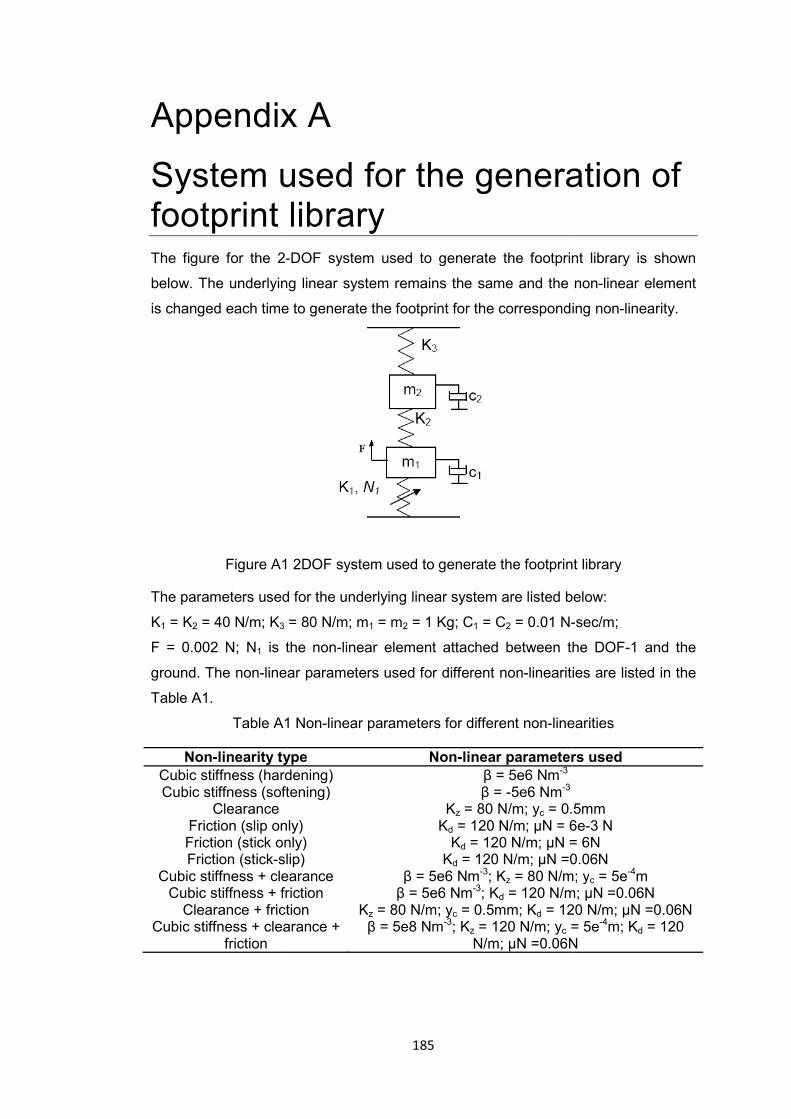
Appendix
System ufootprint The figure for the 2-
below. The underlyin
is changed each time
Figure A1
The parameters used
K1 = K2 = 40 N/m; K3
F = 0.002 N; N1 is t
ground. The non-line
Table A1.
Table A1
Non-linearity tyCubic stiffness (hardCubic stiffness (soft
Clearance Friction (slip onFriction (stick onFriction (stick-s
Cubic stiffness + cleCubic stiffness + fr
Clearance + frictCubic stiffness + clea
friction
185
x A
used for the generalibrary -DOF system used to generate the footprin
ng linear system remains the same and the
e to generate the footprint for the correspond
1 2DOF system used to generate the footprin
d for the underlying linear system are listed b
= 80 N/m; m1 = m2 = 1 Kg; C1 = C2 = 0.01 N-
the non-linear element attached between t
ear parameters used for different non-linearit
1 Non-linear parameters for different non-line
ype Non-linear parameterdening) β = 5e6 Nm-3 tening) β = -5e6 Nm-3
Kz = 80 N/m; yc = 0.nly) Kd = 120 N/m; µN = 6nly) Kd = 120 N/m; µN =lip) Kd = 120 N/m; µN =0
earance β = 5e6 Nm-3; Kz = 80 N/mriction β = 5e6 Nm-3; Kd = 120 N/mtion Kz = 80 N/m; yc = 0.5mm; Kd = 12arance + β = 5e8 Nm-3; Kz = 120 N/m; yc =
N/m; µN =0.06N
ation of
nt library is shown
non-linear element
ing non-linearity.
nt library
below:
-sec/m;
he DOF-1 and the
ies are listed in the
earities
rs used
5mm 6e-3 N = 6N 0.06N
m; yc = 5e-4m m; µN =0.06N 20 N/m; µN =0.06N = 5e-4m; Kd = 120 N

186
Appendix B
Structures used for the validation
Validation Structure-1: Cantilever beam
A cantilever beam is used as the validation structure-1 for the validation purpose. A
detailed drawing of the structure is shown in the Figure B1.
Figure B1 Validation structure-1: Cantilever beam
The cantilever beam is modelled using FE method with beam elements processing
2 DOFs per node: a translational DOF along Y axis and a rotational DOF about the
Z axis. The excitation force of sinusoidal nature with amplitude 0.001N is applied at
the free end of the beam. The non-linear element is placed at the free end of the
beam.
Validation Structure-2 Cantilever plate
A cantilever plate is used as validation structure-2 for the validation of the
algorithms in the thesis. Figure B2 shows the detail drawing of the structure. The
plate is modelled in FEM using Kirchhoff’s plate elements with 3 DOF per node: a
translational DOF along Z axis and rotations about X and Y axes. The excitation
force of 0.05N is applied to the edge of the plate as shown. The non-linear element
is placed at the corner of the plate. The type of non-linearity is varied during the
validation of different algorithms.

187
Figure B2 Validation structure-2: cantilever plate
The plate is meshed with 36 elements. After imposing the boundary conditions, the
total number of nodes in the model equals 42, with 3 DOFs per node. Table B1 lists
the linear natural frequencies for the first 9 modes.
Table B1 Linear natural frequencies for validation structure-2
Mode Number Natural frequency
(rad/sec)
1 87.2
2 213.8
3 537.8
4 680.9
5 777.8
6 1345.9
7 1548.7
8 1613.9
9 1782.1
Figure B3 shows the mode shapes of the first 9 modes of the structure.

188
Figure B3 Mode shapes of validation structure-2
Validation Structure-3 Pyramid
A pyramid-like structure is used as Validation structure-3 for the validation of the
identification method proposed for base-excited structure in Chapter 8. It consists of
4 beams joined at the top to form a tower. The beams are grounded at the base on
a rigid platform. Figure B4 shows the engineering drawing of the structure. The
material properties for the beams in the structure are listed in Table B2.
Table B2 Material properties for the beams in Validation Structure-3
Material property Value
Density (ρ) 7800 kg/m3
Poisson’s ratio (ν) 0.28
Young’s modulus of elasticity (E) 2.1×10¹¹ N/m2
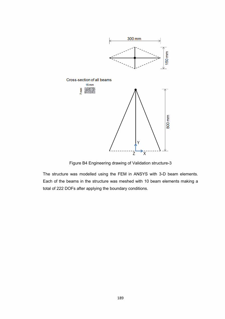
189
Figure B4 Engineering drawing of Validation structure-3
The structure was modelled using the FEM in ANSYS with 3-D beam elements.
Each of the beams in the structure was meshed with 10 beam elements making a
total of 222 DOFs after applying the boundary conditions.

190
Appendix C
Details of ‘1203 structure’ The engineering drawings of ‘1203 structure’ are shown below in Figure C1. The
properties of Aluminum alloy used in the simulation are as follow:
Young’s modulus of elasticity, E = 71×109 N/m2
Density of the material, ρ = 2800 Kg/m3
Poisson’s ratio, ν = 0.3
Figure C1 Engineering drawing of 1203 structure
The natural frequencies for the underlying linear structure are presented in Table C1.
Table C1 Natural frequencies of the underlying linear structure
Mode No Natural frequency (Hz) Mode No Natural
frequency (Hz) 1 8.905 8 137.94 2 10.711 9 166.34 3 38.166 10 187.12 4 41.236 11 188.71 5 62.209 12 198.33 6 119.10 13 210.06 7 131.70 14 249.41

191
Appendix D
MACE structure details and repeatability test results
D.1. Material properties and the FE model mesh information
The following table gives the details of the material properties for different
components of the MACE sub-assembly and the mesh-sizes used in the FE models
of the sub-assembly.
Table D1 Details of the material properties and FE model mesh
Component Material
Material properties Maximum element edge length (mm)
E
(N/m2)
ρ
(Kg/m3) ν
Case Aluminum alloy 7×10¹⁰ 2724.7 0.33 40
Collar Aluminum alloy 7×10¹⁰ 2800 0.33 20
Body Aluminum alloy 7×10¹⁰ 2747.3 0.33 40
Retaining nut Stainless steel 1.95×10¹¹ 7272.1 0.29 3
D.2. Repeatability tests for non-linear measurements
For non-linear systems, sometimes it is difficult to get repeatable measurements. In
order to perform proper system identification, it is necessary to have measurement
data which is consistent and repeatable. For the data used in thesis, repeatability
tests were performed to check the consistency of the experimental setup. The
repeatability tests were performed at three excitation levels. At each level, the
measurements were taken by disassembling the structure completely and again
assembling it with the designated torque. Figure D1, D2 and D3 show the results of
the repeatability tests performed at 0.5N, 3N, and 5N excitation force respectively.

192
Figure D1 Repeatability test results at force level 0.5N
Figure D2 Repeatability test results at force level of 3N
Figure D3 repeatability test results at force level of 5N