moving beyond linearity - | stanford lagunita · moving beyond linearity the truth is never linear!...
TRANSCRIPT

Moving Beyond Linearity
The truth is never linear!
Or almost never!
But often the linearity assumption is good enough.
When its not . . .
• polynomials,
• step functions,
• splines,
• local regression, and
• generalized additive models
offer a lot of flexibility, without losing the ease andinterpretability of linear models.
1 / 23

Moving Beyond Linearity
The truth is never linear!Or almost never!
But often the linearity assumption is good enough.
When its not . . .
• polynomials,
• step functions,
• splines,
• local regression, and
• generalized additive models
offer a lot of flexibility, without losing the ease andinterpretability of linear models.
1 / 23

Polynomial Regression
yi = β0 + β1xi + β2x2i + β3x
3i + . . .+ βdx
di + εi
20 30 40 50 60 70 80
50
10
01
50
20
02
50
30
0
Age
Wa
ge
Degree−4 Polynomial
20 30 40 50 60 70 80
0.0
00
.05
0.1
00
.15
0.2
0
Age
| | || | ||| | ||| | | ||| | || | | |||
|
|| || ||| | | | || || || | || |
|
|| | | |
|
| || || || | | || | ||| || ||| | | |
|
| || | ||| || | || |||| || || ||| || || ||| |||| || | | | ||
|
|| || ||| ||| || || ||| || ||| | || ||| |||| ||| || | | | ||| || |||| |||| || || | ||||| | || || || | ||| | || ||| || | || ||
|
||| | || | || || | || | ||| || || | || ||| |
|
| | |||| ||| | || | |||| ||| || || ||| | | || || |||||| || | || || | || || | | || || || | || ||| || | || || ||||| ||||| || || || || | |||| || || ||| | || || || |
|
| |||| ||| || || || ||| | | ||
|
|| |
|
| || || || ||| || || | || || || | || ||| || | ||| || | || || || | |||| || | |||| | |||| || | | | ||||
|
| || || || || || |
|
| |||| || || |||| | || || || ||| | || |||| || |
|
| | |||| || || || |
|
|| |||| ||| ||
|
||| || |||| | || || | | |||
|
||| || | || | || | || || ||||| | | ||| |
|
| | || || ||| ||| | || |
|
|| | || || | |||| || | || || | ||| || || || || |||| || | ||||| | | |||| | || ||| || ||| |
|
| ||| | || || | | || |
|
| | | ||| |||| || || | | || || | |||| | | | ||| | || | |||| ||| | |
|
|| ||||| ||| | | || || || || || || || |
|
| || || || | ||| || || | || || |||| |||| |
|
| || || ||| || | | ||| || || | ||| ||| || || |
|
||| || || || || || | | ||| | || ||| || || | |||| || | |
|
|| || ||||| || | || || ||| | ||| | || ||| ||||| || ||||| ||| | ||| ||| | || || || ||| || || | | || |
|
| || |||| ||| | |||
|
| | | | || | ||| | | || | |||| || ||| || | ||| || | ||| ||
|
|| || |||| | ||| | || | | ||| |||| || ||| || || || | | || | || | || || || || | | || || | |
|
|| ||| ||||| ||| ||| || ||||| || || | ||| || | | || | ||| | | ||| || || || || | ||| ||| || || |||
|
| || || ||| | | ||| | |||| | || || ||||
|
| | || | || | || | |||
|
| || || ||| | | ||| ||| | || ||| || || ||| | |||| | ||| | ||| | || | || | || | | || || || || || |||| || | | || | | | |||| || | ||| | || ||| || || ||| ||
|
||| ||| | || || || | | || | || || || || || || | || || | || || |
|
| || ||| || |
| |
| ||| | || || |
|
| |||| ||| | |||| ||
|
| ||| ||| ||| |||| |
|
| || || || || ||| | | | || || | ||| || | || | || | |||| | ||| ||| ||
|
| | ||||| ||| | | || || | | |||| | |||| ||| ||| | || | || || || | || | || || ||| | || ||| | || || ||| | | | |||| | || | | ||| ||| |||| | | ||| | |||| | || | || || | ||
|
| || ||||| || ||| ||| || | | ||||| || |||| || | | ||| | || || || ||| |||| |||| | | || || || | ||| | || || || | | || || || |||| || ||| || ||| || |
|
| || || |||| || | ||| | ||| || | || |||| |||| ||| | | | || ||| | || | | ||
|
|| |||| ||| ||| || | | |||| ||| |||| || |||| || || ||| |||| | ||| | |
|
|| | || || || | ||| | || ||| || ||| | || || ||| | || || || | || ||| | || || |||| || || | || ||| ||
|
|| || | || || || | || | ||| | ||| || | || || ||| || ||| ||| || | || || | | || || || ||| || || || | ||| || | |||
|
|| | |
|
||| | | | || ||| || | ||||| | | || || || | | || || || | | || ||| | |||| |
|
||||| | | | || || | | ||| || | | || | || | ||| || |||| | ||| | || || ||||| | || ||| ||| | || || || || || ||| | ||||| || || ||| ||| || | | || || || ||
|
| || | | || | || || | || || || | |||| | | | ||| | | ||
|
| | || ||
|
|| | | ||| || ||| || || | || || || || | | || ||| || ||| || || || ||| | ||| || ||| || ||| | ||| | | | || || | ||| ||| || | ||
|
|||| |
|
|| | |||| ||| | || || ||| || ||| | |||| || |
|
|| ||| ||| | ||| | || | | | ||| || | || || ||| | | | ||| || || ||| || | ||| | || |||| | |||| | ||| || || || || || | ||| || || | | ||| || || |||| ||| || | || ||| || | ||| |
|
| || | |||
|
| | || || | ||| || |
|
| | ||| || || || | | || | ||| | | ||| || | | || | | || ||||| || || |||| | ||| | | || || | | || | | |
|
|| || |||| | || |||| |
||
| | | ||||| |||
|
|| |||| | |||| || |
|
| | || ||||| ||||| | || || || | || ||| ||| | || ||| || ||| || | || || ||| || | | | || || ||| | || || | || || |
|
| || ||
|
|| || ||| || | | | || |||| || |||| ||| || |||| || || | ||| | |||
|
|| ||| | |
| |
|| || | ||| || ||| | | |||| | ||| | |||| || ||| || || | ||| | ||| | |||| || | || |||| | ||||| ||| | | ||| | ||| || ||| || | ||| || ||| | ||| || | ||| | | || || || || | ||| || || || |||| ||| | ||| || || |||| || |||
|
| |||
|
| ||
|
| |
|
|
|
| | | || || |||
|
|||| ||
|
|| || || || || || | | ||||| | ||| || | ||| ||| || ||| || | | || || | || | || ||| |||| || || ||| |||| ||| ||| ||| | | || |
|
| ||| || || || ||| ||| | ||| | || || ||| || || ||| ||
|
| ||| | || | || || |||| || ||| || | | ||| || | || ||| || || | || ||
|
| | ||| || | | | ||
|
| | || | | ||| | || | || | ||| || || ||| | | || |
|
|| ||| || || | || || |||| || || || | || || | || ||| | || ||| | || ||| || || | | || || ||| || || || ||| |||| |
Pr(Wage>
250|A
ge)
2 / 23

Details
• Create new variables X1 = X, X2 = X2, etc and then treatas multiple linear regression.
• Not really interested in the coefficients; more interested inthe fitted function values at any value x0:
f(x0) = β0 + β1x0 + β2x20 + β3x
30 + β4x
40.
• Since f(x0) is a linear function of the β`, can get a simpleexpression for pointwise-variances Var[f(x0)] at anyvalue x0. In the figure we have computed the fit andpointwise standard errors on a grid of values for x0. Weshow f(x0)± 2 · se[f(x0)].
• We either fix the degree d at some reasonably low value,else use cross-validation to choose d.
3 / 23

Details continued
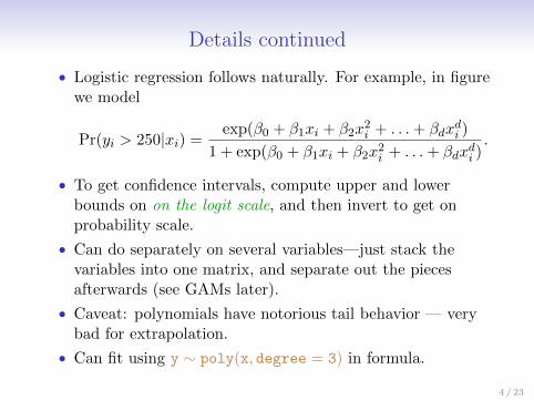
• Logistic regression follows naturally. For example, in figurewe model
Pr(yi > 250|xi) =exp(β0 + β1xi + β2x
2i + . . .+ βdx
di )
1 + exp(β0 + β1xi + β2x2i + . . .+ βdxdi ).
• To get confidence intervals, compute upper and lowerbounds on on the logit scale, and then invert to get onprobability scale.
• Can do separately on several variables—just stack thevariables into one matrix, and separate out the piecesafterwards (see GAMs later).
• Caveat: polynomials have notorious tail behavior — verybad for extrapolation.
• Can fit using y ∼ poly(x, degree = 3) in formula.
4 / 23

Details continued
• Logistic regression follows naturally. For example, in figurewe model
Pr(yi > 250|xi) =exp(β0 + β1xi + β2x
2i + . . .+ βdx
di )
1 + exp(β0 + β1xi + β2x2i + . . .+ βdxdi ).
• To get confidence intervals, compute upper and lowerbounds on on the logit scale, and then invert to get onprobability scale.
• Can do separately on several variables—just stack thevariables into one matrix, and separate out the piecesafterwards (see GAMs later).
• Caveat: polynomials have notorious tail behavior — verybad for extrapolation.
• Can fit using y ∼ poly(x, degree = 3) in formula.
4 / 23

Step FunctionsAnother way of creating transformations of a variable — cutthe variable into distinct regions.
C1(X) = I(X < 35), C2(X) = I(35 ≤ X < 50), . . . , C3(X) = I(X ≥ 65)
20 30 40 50 60 70 80
50
10
01
50
20
02
50
30
0
Age
Wa
ge
Piecewise Constant
20 30 40 50 60 70 80
0.0
00
.05
0.1
00
.15
0.2
0
Age
| | || | ||| | ||| | | ||| | || | | |||
|
|| || ||| | | | || || || | || |
|
|| | | |
|
| || || || | | || | ||| || ||| | | |
|
| || | ||| || | || |||| || || ||| || || ||| |||| || | | | ||
|
|| || ||| ||| || || ||| || ||| | || ||| |||| ||| || | | | ||| || |||| |||| || || | ||||| | || || || | ||| | || ||| || | || ||
|
||| | || | || || | || | ||| || || | || ||| |
|
| | |||| ||| | || | |||| ||| || || ||| | | || || |||||| || | || || | || || | | || || || | || ||| || | || || ||||| ||||| || || || || | |||| || || ||| | || || || |
|
| |||| ||| || || || ||| | | ||
|
|| |
|
| || || || ||| || || | || || || | || ||| || | ||| || | || || || | |||| || | |||| | |||| || | | | ||||
|
| || || || || || |
|
| |||| || || |||| | || || || ||| | || |||| || |
|
| | |||| || || || |
|
|| |||| ||| ||
|
||| || |||| | || || | | |||
|
||| || | || | || | || || ||||| | | ||| |
|
| | || || ||| ||| | || |
|
|| | || || | |||| || | || || | ||| || || || || |||| || | ||||| | | |||| | || ||| || ||| |
|
| ||| | || || | | || |
|
| | | ||| |||| || || | | || || | |||| | | | ||| | || | |||| ||| | |
|
|| ||||| ||| | | || || || || || || || |
|
| || || || | ||| || || | || || |||| |||| |
|
| || || ||| || | | ||| || || | ||| ||| || || |
|
||| || || || || || | | ||| | || ||| || || | |||| || | |
|
|| || ||||| || | || || ||| | ||| | || ||| ||||| || ||||| ||| | ||| ||| | || || || ||| || || | | || |
|
| || |||| ||| | |||
|
| | | | || | ||| | | || | |||| || ||| || | ||| || | ||| ||
|
|| || |||| | ||| | || | | ||| |||| || ||| || || || | | || | || | || || || || | | || || | |
|
|| ||| ||||| ||| ||| || ||||| || || | ||| || | | || | ||| | | ||| || || || || | ||| ||| || || |||
|
| || || ||| | | ||| | |||| | || || ||||
|
| | || | || | || | |||
|
| || || ||| | | ||| ||| | || ||| || || ||| | |||| | ||| | ||| | || | || | || | | || || || || || |||| || | | || | | | |||| || | ||| | || ||| || || ||| ||
|
||| ||| | || || || | | || | || || || || || || | || || | || || |
|
| || ||| || |
| |
| ||| | || || |
|
| |||| ||| | |||| ||
|
| ||| ||| ||| |||| |
|
| || || || || ||| | | | || || | ||| || | || | || | |||| | ||| ||| ||
|
| | ||||| ||| | | || || | | |||| | |||| ||| ||| | || | || || || | || | || || ||| | || ||| | || || ||| | | | |||| | || | | ||| ||| |||| | | ||| | |||| | || | || || | ||
|
| || ||||| || ||| ||| || | | ||||| || |||| || | | ||| | || || || ||| |||| |||| | | || || || | ||| | || || || | | || || || |||| || ||| || ||| || |
|
| || || |||| || | ||| | ||| || | || |||| |||| ||| | | | || ||| | || | | ||
|
|| |||| ||| ||| || | | |||| ||| |||| || |||| || || ||| |||| | ||| | |
|
|| | || || || | ||| | || ||| || ||| | || || ||| | || || || | || ||| | || || |||| || || | || ||| ||
|
|| || | || || || | || | ||| | ||| || | || || ||| || ||| ||| || | || || | | || || || ||| || || || | ||| || | |||
|
|| | |
|
||| | | | || ||| || | ||||| | | || || || | | || || || | | || ||| | |||| |
|
||||| | | | || || | | ||| || | | || | || | ||| || |||| | ||| | || || ||||| | || ||| ||| | || || || || || ||| | ||||| || || ||| ||| || | | || || || ||
|
| || | | || | || || | || || || | |||| | | | ||| | | ||
|
| | || ||
|
|| | | ||| || ||| || || | || || || || | | || ||| || ||| || || || ||| | ||| || ||| || ||| | ||| | | | || || | ||| ||| || | ||
|
|||| |
|
|| | |||| ||| | || || ||| || ||| | |||| || |
|
|| ||| ||| | ||| | || | | | ||| || | || || ||| | | | ||| || || ||| || | ||| | || |||| | |||| | ||| || || || || || | ||| || || | | ||| || || |||| ||| || | || ||| || | ||| |
|
| || | |||
|
| | || || | ||| || |
|
| | ||| || || || | | || | ||| | | ||| || | | || | | || ||||| || || |||| | ||| | | || || | | || | | |
|
|| || |||| | || |||| |
||
| | | ||||| |||
|
|| |||| | |||| || |
|
| | || ||||| ||||| | || || || | || ||| ||| | || ||| || ||| || | || || ||| || | | | || || ||| | || || | || || |
|
| || ||
|
|| || ||| || | | | || |||| || |||| ||| || |||| || || | ||| | |||
|
|| ||| | |
| |
|| || | ||| || ||| | | |||| | ||| | |||| || ||| || || | ||| | ||| | |||| || | || |||| | ||||| ||| | | ||| | ||| || ||| || | ||| || ||| | ||| || | ||| | | || || || || | ||| || || || |||| ||| | ||| || || |||| || |||
|
| |||
|
| ||
|
| |
|
|
|
| | | || || |||
|
|||| ||
|
|| || || || || || | | ||||| | ||| || | ||| ||| || ||| || | | || || | || | || ||| |||| || || ||| |||| ||| ||| ||| | | || |
|
| ||| || || || ||| ||| | ||| | || || ||| || || ||| ||
|
| ||| | || | || || |||| || ||| || | | ||| || | || ||| || || | || ||
|
| | ||| || | | | ||
|
| | || | | ||| | || | || | ||| || || ||| | | || |
|
|| ||| || || | || || |||| || || || | || || | || ||| | || ||| | || ||| || || | | || || ||| || || || ||| |||| |
Pr(Wage>
250|A
ge)
5 / 23
Step functions continued
• Easy to work with. Creates a series of dummy variablesrepresenting each group.
• Useful way of creating interactions that are easy tointerpret. For example, interaction effect of Year and Age:
I(Year < 2005) · Age, I(Year ≥ 2005) · Age
would allow for different linear functions in each agecategory.
• In R: I(year < 2005) or cut(age, c(18, 25, 40, 65, 90)).
• Choice of cutpoints or knots can be problematic. Forcreating nonlinearities, smoother alternatives such assplines are available.
6 / 23

Piecewise Polynomials
• Instead of a single polynomial in X over its whole domain,we can rather use different polynomials in regions definedby knots. E.g. (see figure)
yi =
{β01 + β11xi + β21x
2i + β31x
3i + εi if xi < c;
β02 + β12xi + β22x2i + β32x
3i + εi if xi ≥ c.
• Better to add constraints to the polynomials, e.g.continuity.
• Splines have the “maximum” amount of continuity.
7 / 23

20 30 40 50 60 70
50
100
150
200
250
Age
Wage
Piecewise Cubic
20 30 40 50 60 70
50
100
150
200
250
Age
Wage
Continuous Piecewise Cubic
20 30 40 50 60 70
50
100
150
200
250
Age
Wage
Cubic Spline
20 30 40 50 60 70
50
100
150
200
250
Age
Wage
Linear Spline
8 / 23

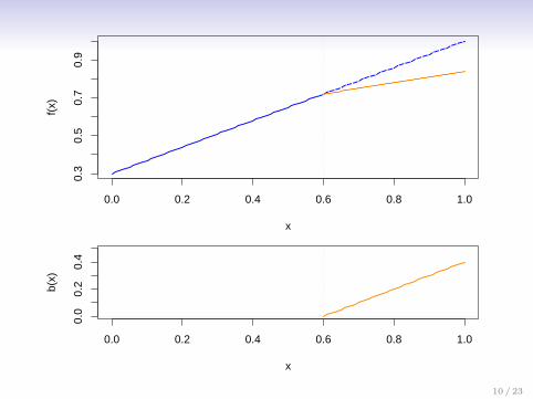
Linear SplinesA linear spline with knots at ξk, k = 1, . . . ,K is a piecewiselinear polynomial continuous at each knot.
We can represent this model as
yi = β0 + β1b1(xi) + β2b2(xi) + · · ·+ βK+3bK+3(xi) + εi,
where the bk are basis functions.
b1(xi) = xi
bk+1(xi) = (xi − ξk)+, k = 1, . . . ,K
Here the ()+ means positive part; i.e.
(xi − ξk)+ =
{xi − ξk if xi > ξk
0 otherwise
9 / 23
0.0 0.2 0.4 0.6 0.8 1.0
0.3
0.5
0.7
0.9
x
f(x)
0.0 0.2 0.4 0.6 0.8 1.0
0.0
0.2
0.4
x
b(x)
10 / 23
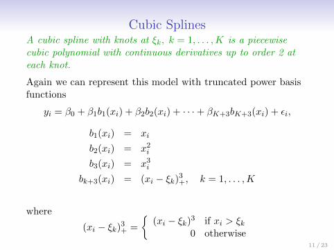
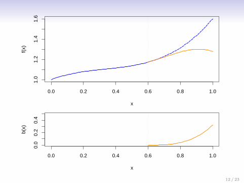
Cubic SplinesA cubic spline with knots at ξk, k = 1, . . . ,K is a piecewisecubic polynomial with continuous derivatives up to order 2 ateach knot.
Again we can represent this model with truncated power basisfunctions
yi = β0 + β1b1(xi) + β2b2(xi) + · · ·+ βK+3bK+3(xi) + εi,
b1(xi) = xi
b2(xi) = x2i
b3(xi) = x3i
bk+3(xi) = (xi − ξk)3+, k = 1, . . . ,K
where
(xi − ξk)3+ =
{(xi − ξk)3 if xi > ξk
0 otherwise11 / 23
0.0 0.2 0.4 0.6 0.8 1.0
1.0
1.2
1.4
1.6
x
f(x)
0.0 0.2 0.4 0.6 0.8 1.0
0.0
0.2
0.4
x
b(x)
12 / 23

Natural Cubic SplinesA natural cubic spline extrapolates linearly beyond theboundary knots. This adds 4 = 2× 2 extra constraints, andallows us to put more internal knots for the same degrees offreedom as a regular cubic spline.
20 30 40 50 60 70
50
10
01
50
20
02
50
Age
Wa
ge
Natural Cubic Spline
Cubic Spline
13 / 23

Fitting splines in R is easy: bs(x, ...) for any degree splines,and ns(x, ...) for natural cubic splines, in package splines.
20 30 40 50 60 70 80
50
10
01
50
20
02
50
30
0
Age
Wa
ge
Natural Cubic Spline
20 30 40 50 60 70 80
0.0
00
.05
0.1
00
.15
0.2
0
Age
| | || | ||| | ||| | | ||| | || | | |||
|
|| || ||| | | | || || || | || |
|
|| | | |
|
| || || || | | || | ||| || ||| | | |
|
| || | ||| || | || |||| || || ||| || || ||| |||| || | | | ||
|
|| || ||| ||| || || ||| || ||| | || ||| |||| ||| || | | | ||| || |||| |||| || || | ||||| | || || || | ||| | || ||| || | || ||
|
||| | || | || || | || | ||| || || | || ||| |
|
| | |||| ||| | || | |||| ||| || || ||| | | || || |||||| || | || || | || || | | || || || | || ||| || | || || ||||| ||||| || || || || | |||| || || ||| | || || || |
|
| |||| ||| || || || ||| | | ||
|
|| |
|
| || || || ||| || || | || || || | || ||| || | ||| || | || || || | |||| || | |||| | |||| || | | | ||||
|
| || || || || || |
|
| |||| || || |||| | || || || ||| | || |||| || |
|
| | |||| || || || |
|
|| |||| ||| ||
|
||| || |||| | || || | | |||
|
||| || | || | || | || || ||||| | | ||| |
|
| | || || ||| ||| | || |
|
|| | || || | |||| || | || || | ||| || || || || |||| || | ||||| | | |||| | || ||| || ||| |
|
| ||| | || || | | || |
|
| | | ||| |||| || || | | || || | |||| | | | ||| | || | |||| ||| | |
|
|| ||||| ||| | | || || || || || || || |
|
| || || || | ||| || || | || || |||| |||| |
|
| || || ||| || | | ||| || || | ||| ||| || || |
|
||| || || || || || | | ||| | || ||| || || | |||| || | |
|
|| || ||||| || | || || ||| | ||| | || ||| ||||| || ||||| ||| | ||| ||| | || || || ||| || || | | || |
|
| || |||| ||| | |||
|
| | | | || | ||| | | || | |||| || ||| || | ||| || | ||| ||
|
|| || |||| | ||| | || | | ||| |||| || ||| || || || | | || | || | || || || || | | || || | |
|
|| ||| ||||| ||| ||| || ||||| || || | ||| || | | || | ||| | | ||| || || || || | ||| ||| || || |||
|
| || || ||| | | ||| | |||| | || || ||||
|
| | || | || | || | |||
|
| || || ||| | | ||| ||| | || ||| || || ||| | |||| | ||| | ||| | || | || | || | | || || || || || |||| || | | || | | | |||| || | ||| | || ||| || || ||| ||
|
||| ||| | || || || | | || | || || || || || || | || || | || || |
|
| || ||| || |
| |
| ||| | || || |
|
| |||| ||| | |||| ||
|
| ||| ||| ||| |||| |
|
| || || || || ||| | | | || || | ||| || | || | || | |||| | ||| ||| ||
|
| | ||||| ||| | | || || | | |||| | |||| ||| ||| | || | || || || | || | || || ||| | || ||| | || || ||| | | | |||| | || | | ||| ||| |||| | | ||| | |||| | || | || || | ||
|
| || ||||| || ||| ||| || | | ||||| || |||| || | | ||| | || || || ||| |||| |||| | | || || || | ||| | || || || | | || || || |||| || ||| || ||| || |
|
| || || |||| || | ||| | ||| || | || |||| |||| ||| | | | || ||| | || | | ||
|
|| |||| ||| ||| || | | |||| ||| |||| || |||| || || ||| |||| | ||| | |
|
|| | || || || | ||| | || ||| || ||| | || || ||| | || || || | || ||| | || || |||| || || | || ||| ||
|
|| || | || || || | || | ||| | ||| || | || || ||| || ||| ||| || | || || | | || || || ||| || || || | ||| || | |||
|
|| | |
|
||| | | | || ||| || | ||||| | | || || || | | || || || | | || ||| | |||| |
|
||||| | | | || || | | ||| || | | || | || | ||| || |||| | ||| | || || ||||| | || ||| ||| | || || || || || ||| | ||||| || || ||| ||| || | | || || || ||
|
| || | | || | || || | || || || | |||| | | | ||| | | ||
|
| | || ||
|
|| | | ||| || ||| || || | || || || || | | || ||| || ||| || || || ||| | ||| || ||| || ||| | ||| | | | || || | ||| ||| || | ||
|
|||| |
|
|| | |||| ||| | || || ||| || ||| | |||| || |
|
|| ||| ||| | ||| | || | | | ||| || | || || ||| | | | ||| || || ||| || | ||| | || |||| | |||| | ||| || || || || || | ||| || || | | ||| || || |||| ||| || | || ||| || | ||| |
|
| || | |||
|
| | || || | ||| || |
|
| | ||| || || || | | || | ||| | | ||| || | | || | | || ||||| || || |||| | ||| | | || || | | || | | |
|
|| || |||| | || |||| |
||
| | | ||||| |||
|
|| |||| | |||| || |
|
| | || ||||| ||||| | || || || | || ||| ||| | || ||| || ||| || | || || ||| || | | | || || ||| | || || | || || |
|
| || ||
|
|| || ||| || | | | || |||| || |||| ||| || |||| || || | ||| | |||
|
|| ||| | |
| |
|| || | ||| || ||| | | |||| | ||| | |||| || ||| || || | ||| | ||| | |||| || | || |||| | ||||| ||| | | ||| | ||| || ||| || | ||| || ||| | ||| || | ||| | | || || || || | ||| || || || |||| ||| | ||| || || |||| || |||
|
| |||
|
| ||
|
| |
|
|
|
| | | || || |||
|
|||| ||
|
|| || || || || || | | ||||| | ||| || | ||| ||| || ||| || | | || || | || | || ||| |||| || || ||| |||| ||| ||| ||| | | || |
|
| ||| || || || ||| ||| | ||| | || || ||| || || ||| ||
|
| ||| | || | || || |||| || ||| || | | ||| || | || ||| || || | || ||
|
| | ||| || | | | ||
|
| | || | | ||| | || | || | ||| || || ||| | | || |
|
|| ||| || || | || || |||| || || || | || || | || ||| | || ||| | || ||| || || | | || || ||| || || || ||| |||| |
Pr(Wage>
250|A
ge)
14 / 23

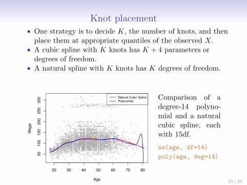
Knot placement• One strategy is to decide K, the number of knots, and then
place them at appropriate quantiles of the observed X.• A cubic spline with K knots has K + 4 parameters or
degrees of freedom.• A natural spline with K knots has K degrees of freedom.
20 30 40 50 60 70 80
50
100
150
200
250
300
Age
Wage
Natural Cubic Spline
PolynomialComparison of adegree-14 polyno-mial and a naturalcubic spline, eachwith 15df.
ns(age, df=14)
poly(age, deg=14)
15 / 23

Smoothing Splines
This section is a little bit mathematical
Consider this criterion for fitting a smooth function g(x) tosome data:
minimizeg∈S
n∑i=1
(yi − g(xi))2 + λ
∫g′′(t)2dt
• The first term is RSS, and tries to make g(x) match thedata at each xi.
• The second term is a roughness penalty and controls howwiggly g(x) is. It is modulated by the tuning parameterλ ≥ 0.
• The smaller λ, the more wiggly the function, eventuallyinterpolating yi when λ = 0.
• As λ→∞, the function g(x) becomes linear.
16 / 23

Smoothing Splines continuedThe solution is a natural cubic spline, with a knot at everyunique value of xi. The roughness penalty still controls theroughness via λ.
Some details
• Smoothing splines avoid the knot-selection issue, leaving asingle λ to be chosen.
• The algorithmic details are too complex to describe here.In R, the function smooth.spline() will fit a smoothingspline.
• The vector of n fitted values can be written as gλ = Sλy,where Sλ is a n× n matrix (determined by the xi and λ).
• The effective degrees of freedom are given by
dfλ =
n∑i=1
{Sλ}ii.
17 / 23

Smoothing Splines continued — choosing λ
• We can specify df rather than λ!
In R: smooth.spline(age, wage, df = 10)
• The leave-one-out (LOO) cross-validated error is given by
RSScv(λ) =n∑i=1
(yi − g(−i)λ (xi))2 =
n∑i=1
[yi − gλ(xi)
1− {Sλ}ii
]2.
In R: smooth.spline(age, wage)
18 / 23

Smoothing Splines continued — choosing λ
• We can specify df rather than λ!
In R: smooth.spline(age, wage, df = 10)
• The leave-one-out (LOO) cross-validated error is given by
RSScv(λ) =
n∑i=1
(yi − g(−i)λ (xi))2 =
n∑i=1
[yi − gλ(xi)
1− {Sλ}ii
]2.
In R: smooth.spline(age, wage)
18 / 23

20 30 40 50 60 70 80
050
100
200
300
Age
WageSmoothing Spline
16 Degrees of Freedom
6.8 Degrees of Freedom (LOOCV)
19 / 23

Local Regression
0.0 0.2 0.4 0.6 0.8 1.0
−1.0
−0.5
0.0
0.5
1.0
1.5
O
O
O
O
O
OO
O
O
O
O
O
O
O
O
OOO
O
O
O
O
O
O
O
O
OO
O
O
OO
O
O
O
O
O
O
OO
O
O
O
O
O
O
O
O
O
O
OO
O
O
O
O
O
OO
O
O
O
O
OO
O
O
OO
O
O
O
OO
O
O
O
O
O
O
O
OO
O
O
O
OO
O
O
O
O
OO
O
O
O
O
O
O
O
O
O
O
O
OO
O
O
O
O
O
O
O
O
OOO
O
O
O
O
0.0 0.2 0.4 0.6 0.8 1.0
−1.0
−0.5
0.0
0.5
1.0
1.5
O
O
O
O
O
OO
O
O
O
O
O
O
O
O
OOO
O
O
O
O
O
O
O
O
OO
O
O
OO
O
O
O
O
O
O
OO
O
O
O
O
O
O
O
O
O
O
OO
O
O
O
O
O
OO
O
O
O
O
OO
O
O
OO
O
O
O
OO
O
O
O
O
O
O
O
OO
O
O
O
OO
O
O
O
O
OO
O
O
O
O
O
O
O
O
O
O
O
OO
O
O
OO
O
O
O
O
O
O
OO
O
O
O
O
O
O
O
O
O
O
OO
O
O
O
O
O
OO
O
O
O
O
OO
O
O
OO
O
O
Local Regression
With a sliding weight function, we fit separate linear fits overthe range of X by weighted least squares.See text for more details, and loess() function in R.
20 / 23

Generalized Additive Models
Allows for flexible nonlinearities in several variables, but retainsthe additive structure of linear models.
yi = β0 + f1(xi1) + f2(xi2) + · · ·+ fp(xip) + εi.
2003 2005 2007 2009
−3
0−
20
−1
00
10
20
30
20 30 40 50 60 70 80
−5
0−
40
−3
0−
20
−1
00
10
20
−3
0−
20
−1
00
10
20
30
40
<HS HS <Coll Coll >Coll
f 1(year)
f 2(age)
f 3(edu
cation)
year ageeducation
21 / 23

GAM details
• Can fit a GAM simply using, e.g. natural splines:
lm(wage ∼ ns(year, df = 5) + ns(age, df = 5) + education)
• Coefficients not that interesting; fitted functions are. Theprevious plot was produced using plot.gam.
• Can mix terms — some linear, some nonlinear — and useanova() to compare models.
• Can use smoothing splines or local regression as well:
gam(wage ∼ s(year, df = 5) + lo(age, span = .5) + education)
• GAMs are additive, although low-order interactions can beincluded in a natural way using, e.g. bivariate smoothers orinteractions of the form ns(age,df=5):ns(year,df=5).
22 / 23

GAMs for classification
log
(p(X)
1− p(X)
)= β0 + f1(X1) + f2(X2) + · · ·+ fp(Xp).
2003 2005 2007 2009
−4
−2
02
4
20 30 40 50 60 70 80
−8
−6
−4
−2
02
−4
−2
02
4
HS <Coll Coll >Coll
f 1(year)
f 2(age)
f 3(edu
cation)
year ageeducation
gam(I(wage > 250) ∼ year+ s(age, df = 5) + education, family = binomial)
23 / 23