strain-response characterization for unbonded concrete
TRANSCRIPT
The Pennsylvania State University
The Graduate School
College of Engineering
STRAIN-RESPONSE CHARACTERIZATION FOR UNBONDED CONCRETE
OVERLAYS SUBJECTED TO
HEAVY AIRCRAFT GEAR WITH MULTIPLE AXLES
A Thesis in
Civil Engineering
by.
Vishal Kumar Singh
© 2010 Vishal K. Singh
Submitted in Partial Fulfillment
of the Requirements
for the Degree of
Master of Science
May 2010

ii
The thesis of Vishal K. Singh was reviewed and approved* by the following:
Shelley Stoffels
Associate Professor of Civil Engineering
Thesis Adviser
Mansour Solaimanian
Senior Research Associate
Farshad Rajabipour
Assistant Professor of Civil Engineering
Angelica Palomino
Assistant Professor of Civil Engineering
Peggy Johnson
Professor of Civil Engineering
Head of the Department of Civil Engineering
*Signatures are on file in the graduate school
iii
ABSTRACT
Concrete pavement performance, with regard to fatigue life, has previously been studied
using strain gages installed in-situ in the pavement, with the primary focus on peak strain
response. This study focuses on identifying and characterizing additional components of
strain responses from unbonded concrete overlays for concrete pavement on airfields, and
relating those strain responses to observed performance. Strain data collected through a
series of full-scale tests at the Federal Aviation Administration (FAA) National Airfield
Pavement Test Facility (NAPTF) are analyzed to observe effects of repeated loading with
heavy aircraft gear with multiple axles on three different structural cross-sections of
unbonded concrete overlays. Components of strain response, such as peak strain,
cumulative area, percent recovery, pre-stress area, post-stress area and duration are
defined; these additional strain response components are analyzed and correlated to peak
strain response. The peak strain is found to be strongly correlated to the cumulative strain
area component of the strain response, but not to other components of the strain response.
Preliminary regression relationships with performance, defined in terms of structural
condition index (SCI), could be established only with peak strain, percent recovery and
number of axles for the top of unbonded overlay, or alternately with area components.
This study provides the foundation for future study of airfield concrete pavement overlay
performance, especially for the subsequent experiment, performed at the same location
with same pavement cross-section but with weakened support conditions.

iv
List of Acronyms
ASTM American Society for Testing and Materials
FAA Federal Aviation Administration
IPRF Innovative Pavement Research Foundation
LPT Linear Position Transducer
NAPTF National Airfield Pavement Test Facility
PCI Pavement Condition Index
QES Quality Engineering Solutions
SCI Structural Condition Index
VBA Visual Basic for Applications

v
TABLE OF CONTENTS
List of Tables………………………………………………………………………….. vii
List of Figures……………………………………………………………………........ xiii
Acknowledgements…………………………………………………………………….. xvi
CHAPTER 1. INTRODUCTION……………………………………………………… 1
1.1. Background…………………………………………………………………. 1
1.2. Objectives………………………………………………………………… 7
1.3. Scope……………………………………………………………………… 8
CHAPTER 2. LITERATURE REVIEW……………………………………………… 10
2.1. Background……………………………………………………………….. 10
2.2. Concrete Properties……………………………………………………….. 10
2.3. Concrete Pavement Fatigue ………………………………………………. 12
2.3.1. Stress Ratio Models……………………………………………….. 12
2.3.2. Slab Fatigue……………………………………………………….. 14
2.3.3. Variable Amplitude Loading……………………………………… 15
2.3.4. Mechanistic Approach……………………………………………. 15
2.3.5. Numerical Approach (Finite-Element Methods)…………………. 16
2.3.6. Fuzzy Logic……………………………………………………….. 16
2.4. Airbus A-380 and Boeing 777……………………………………………. 16
2.5. Current FAA Design Procedure…………………………………………… 18
2.6. Structural Condition Index……………………………………………….. 19
2.7. Strain Gage Characterization…………………………………………….. 19
2.8. Summary of Important Findings from Literature Review………………. 20
CHAPTER 3. FULL-SCALE TESTING OF UNBONDED OVERLAYS ..………….. 22
3.1. NAPTF …………………………………………………………………….. 22
3.2. Pavement Cross-Sections…………………………………………………. 23
3.3. Types of Loading and Aircraft Gears……………………………………. 25
3.4. Instrumentation…………………………………………………………… 29
3.4.1. Strain Gages……………………………………………………….. 29
3.4.2. KM-100B………………………………………………….............. 30
3.5. Performance……………………………………………………………….. 41
CHAPTER 4. METHODOLOGY …………………………………………………... 42
4.1. Overview of Proposed Methodology……………………………………... 42
4.2. Detailed Processing of Data………………………………………………. 43
4.2.1 Data Extraction/Filtering………………………………………….. 44
4.2.2. Responses from Track 0…………………………………………... 44
4.2.3 Matlab Programming……………………………………………… 45
4.2.3.1 Type 1 for North Test Items………………………………. 50
4.2.3.2 Type 2 for North Test Items ………………………………. 53
4.2.3.3 Type 3 for North Test Items ………………………………. 55
4.2.3.4 Type 4 for North Test Items ……………………………… 56
vi
4.2.3.5 Type 1, 2, 3 and 4 for South Test Items…………………… 58
4.2.4 Statistical Analysis…………………………………………………. 60
CHAPTER 5. ANALYSIS …………………………………………………................. 62
5.1. Relationship of Components of Strain Gage Response to Peak Strain….. 62
5.2. Relationships between Peak Strain and other Components of Strain Gage
Response…………………………………………………………………... 72
5.3. Strain Gage Response with Change in Loading and Cross-Sections………. 80
5.4. Performance……………………………………………………………… 86
5.4.1. At the Top of Overlay……………………………………………… 86
5.4.2. At the Bottom of Overlay…………………………………………. 88
5.4.3. At the Top of Underlay……………………………………………. 89
5.4.4. At the Bottom of Underlay……………………………………….. 90
5.5. Summary…………………………………………………………………... 91
CHAPTER 6. CONCLUSIONS AND RECOMMENDATIONS ……………………. 93
6.1. Findings…………………………………………………………………… 93
6.2. Conclusions………………………………………………………………… 96
6.3. Recommendations…………………………………………………….......... 99
REFERENCES………………………………………………………………………… 101
APPENDIX A. Strain gage coordinates and calibration factor…………………….. 111
APPENDIX B. Matlab Codes ……………………………………………………….. 114
APPENDIX C. Mean and Standard Deviation for Selected Gages …………………. 127
APPENDIX D. Performance Prediction………………………………………………. 174

vii
List of Tables
Table 1. Vehicle Passes Utilized for this Study
Table 2. Summary of Design Test Items for Baseline Experiment
Table 3. Loading Sequences
Table 4. KM-100B Specifications (KM Strain transducers manual, 2010).
Table 5. SCI and Date History with First Crack and SCI=80
Table 6. Linear Relation Chart for Even-numbered Passes with Area as Y and Strain as X
for EG-O-N1-1B
Table 7. Linear Relation Chart for Odd-numbered Passes with Area as Y and Strain as X
for EG-O-N1-1B
Table 8. Average, Median and Standard Deviation of the Peak Strain and Area for Odd-
numbered Passes for EG-O-N1-1B.
Table 9. Average, Median and Standard Deviation of the Peak Strain and Area for Even-
numbered for EG-O-N1-1B
Table 10. Linear Relation Chart for Even-numbered Passes with Area as Y and Strain as
X for EG-O-N1-1T
Table 11. Linear Relation Chart for Odd-numbered Passes with Area as Y and Strain as X
for EG-O-N1-1T
Table 12. Average, Median and Standard Deviation of the Peak Strain and Area for Odd-
numbered Passes for for EG-O-N1-1T
Table 13. Average, Median and Standard Deviation of the Peak Strain and Area for Even-
numbered Passes for EG-O-N1-1T
Table 14. Correlation between Peak Strain and Cumulative Area
Table 15. Correlation between % Recovery and Cumulative Area
Table 16. Correlation between Peak Strain and Cumulative Area by Strain Gage
Locations

viii
Table 17. Correlation between Peak Strain and % Recovery by Strain Gage Locations
Table 18. Correlation between Peak Strain and Duration by Strain Gage Locations
Table 19. Correlation between % Recovery and Area by Strain Gage Locations
Table 20. Correlation between Different Components of Peak Responses
Table 21. Regression Statistics for Analysis of % Recovery, Duration and Number of
Axles as Predictors for Peak Strain(Y)
Table 22. Correlation between Different Components of Strain Gage Responses from Top
of Underlay
Table 23. Regression Statistics for Analysis of % Recovery, Duration and Number of
Axles as Predictors for Peak Strain(Y)
Table 24.Mean and Standard Deviation of Components of Gages’ Response at Top of
Overlay
Table 25. Mean and Standard Deviation of Components of Gage Response at Bottom of
Overlay
Table 26. Mean and Standard Deviation of Components of Gage Response at Top of
Underlay
Table 27. Mean and Standard Deviation of Components of Gage Response at Bottom of
Underlay
Table 28. Regression Statistics for Analysis of Performance with Peak Strain and %
Recovery and Number of Axles at Top of Overlay
Table 29. Regression Statistics for Analysis of Performance with Pre-Tension area, Post-
Tension Area, Cumulative Compression Area and Number of Axles at Top of
Overlay
Table 30. Regression Statistics for Analysis of Performance with Pre-Compression Area,
Post-Compression Area, Cumulative Tension Area and Number of Axles at
Bottom of Overlay

ix
Table 31. Regression Statistics for Analysis of Performance with Pre-Tension Area, Post-
Tension Area, Cumulative Compression Area and Number of Axles at Top of
Underlay
Table 32. Regression Statistics for Analysis of Performance with Peak Strain and %
Recovery and Number of Axles at Bottom of Underlay.
Table 33. Regression Statistics for Analysis of Performance with Pre-Compression Area,
Post-Compression Area, Cumulative Tension Area and Number of Axles at
Bottom of Underlay
Table 34. Mean and Standard Deviation of Key Components of Strain Gage Responses
Table 35. Coordinates and Calibration Factor for Strain Gages Installed at Test Item N1
Table 36. Coordinates and Calibration Factor for Strain Gages Installed at Test Item S1
Table 37. Coordinates and Calibration Factor for Strain Gages Installed at Test Item N2
Table 38. Coordinates and Calibration Factor for Strain Gages Installed at Test Item S2
Table 39. Coordinates and Calibration Factor for Strain Gages Installed at Test Item N3
Table 40. Coordinates and Calibration Factor for Strain Gages Installed at Test Item S3
Table 41. Average, Median and Standard Deviation of the Peak Strain(microStrain) and
Area for Even-numbered Passes for EG-U-N1-1 B and EG-U-N1-1 T
Table 42. Linear Relation Chart for Even-numbered Passes for EG-U-N1-1 B and EG-U-
N1-1 T with Area as Y and Strain as X
Table 43. Average, Median and Standard Deviation of the Peak Strain and Area for Odd-
numbered Passes for EG-U-N1-1 B and EG-U-N1-1 T
Table 44. Linear Relation Chart for Odd-numbered Passes for EG-U-N1-1 B and EG-U-
N1-1 T with Area as Y and Strain as X
Table 45. Average, Median and Standard Deviation of the Peak Strain and Area for Odd-
numbered passes for EG-U-N1-3 B and EG-U-N1-3T
Table 46. Linear relation chart for Odd-numbered Passes for EG-U-N1-3 B and EG-U-
N1-3 T with Area as Y and Strain as X

x
Table 47. Average, Median and Standard deviation of the Peak Strain and Area for
Even-numbered passes for EG-O-N2-2 B and EG-O-N2-2 T
Table 48: Linear Relation Chart for Even-numbered Passes for EG-O-N2-2 B and EG-O-
N2-2 T with Area as Y and Strain as X
Table 49. Average, Median and Standard Deviation of the Peak Strain and Area for
Even-numbered passes for EG-U-S1-2 B and EG-U-S1-2 T
Table 50. Linear relation chart for Even-numbered Passes for EG-U-S1-2 B and EG-U-
S1-2 T with Area as Y and Strain as X
Table 51. Average, Median and Standard Deviation of the Peak Strain and Area for Odd-
numbered passes for EG-U-S1-2 B and EG-U-S1-2 T
Table 52. Linear relation chart for Odd-numbered Passes for EG-U-S1-2 B and EG-U-
S1-2 T with Area as Y and Strain as X
Table 53. Average, Median and Standard Deviation of the Peak Strain and Area for
Even-numbered passes for EG-U-S1-3 B and EG-U-S1-3 T
Table 54. Linear relation chart for Even-numbered Passes for EG-U-S1-3 B and EG-U-
S1-3 T with Area as Y and Strain as X
Table 55. Average, Median and Standard Deviation of the Peak Strain and Area for Odd-
numbered passes for EG-U-S1-3 B and EG-U-S1-3 T
Table 56. Linear relation chart for Odd-numbered Passes for EG-U-S1-3 B and EG-U-
S1-3 T with Area as Y and Strain as X
Table 57. Average, Median and Standard Deviation of the Peak Strain and Area for
Even-numbered passes for EG-O-S1-2 B and EG-O-S1-2 T
Table 58. Linear relation chart for Even-numbered Passes for EG-O-S1-2 B and EG-O-
S1-2 T with Area as Y and Strain as X
Table 59. Average, Median and Standard Deviation of the Peak Strain and Area for Odd-
numbered passes for EG-O-S1-2 B and EG-O-S1-2 T
Table 60. Linear relation chart for Odd-numbered Passes for EG-O-S1-1 B and EG-O-
S1-1 T with Area as Y and Strain as X
xi
Table 61. Average, Median and Standard Deviation of the Peak Strain and Area for
Even-numbered passes for EG-O-S1-3 B and EG-O-S1-3 T
Table 62. Linear relation chart for Even-numbered Passes for EG-O-S1-3 B and EG-O-
S1-3 T with Area as Y and Strain as X
Table 63. Average, Median and Standard Deviation of the Peak Strain and Area for
Even-numbered passes for EG-O-N2-2 B and EG-O-N2-2 T
Table 64. Linear relation chart for Even-numbered Passes for EG-O-N2-2 B and EG-O-
N2-2 T with Area as Y and Strain as X
Table 65. Average, Median and Standard Deviation of the Peak Strain and Area for Odd-
numbered passes for EG-O-N2-2 B and EG-O-N2-2 T
Table 66. Linear relation chart for Odd-numbered Passes for EG-O-N2-1 B and EG-O-
N2-1 T with Area as Y and Strain as X
Table 67. Average, Median and Standard Deviation of the Peak Strain and Area for
Even-numbered passes for EG-O-N2-3 B and EG-O-N2-3 T
Table 68. Average, Median and Standard Deviation of the Peak Strain and Area for Odd-
numbered passes for EG-U-S2-1 B and EG-U-S2-1 T
Table 69. Linear relation chart for Odd-numbered Passes for EG-U-S2-1 B and EG-U-
S2-1 T with Area as Y and Strain as X
Table 70. Average, Median and Standard Deviation of the Peak Strain and Area for
Even-numbered passes for EG-U-S2-2 B and EG-U-S2-2 T
Table 71. Linear relation chart for Even-numbered Passes for EG-U-S2-2 B and EG-U-
S2-2 T with Area as Y and Strain as X
Table 72. Average, Median and Standard Deviation of the Peak Strain and Area for Odd-
numbered passes for EG-U-N3-1 B and EG-U-N3-1 T
Table 73. Linear relation chart for Odd-numbered Passes for EG-U-N3-1 B and EG-U-
N3-1 T with Area as Y and Strain as X
Table 74. Average, Median and Standard Deviation of the Peak Strain and Area for
Even-numbered passes for EG-U-N3-2 B and EG-U-N3-2 T
xii
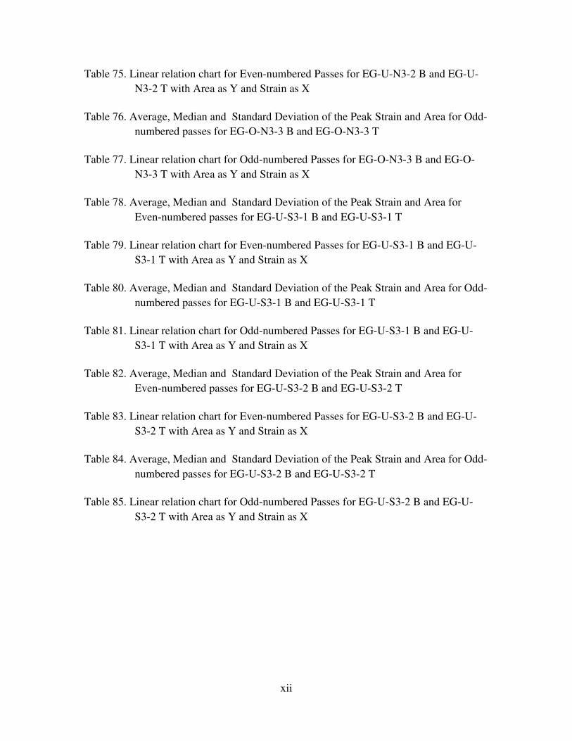
Table 75. Linear relation chart for Even-numbered Passes for EG-U-N3-2 B and EG-U-
N3-2 T with Area as Y and Strain as X
Table 76. Average, Median and Standard Deviation of the Peak Strain and Area for Odd-
numbered passes for EG-O-N3-3 B and EG-O-N3-3 T
Table 77. Linear relation chart for Odd-numbered Passes for EG-O-N3-3 B and EG-O-
N3-3 T with Area as Y and Strain as X
Table 78. Average, Median and Standard Deviation of the Peak Strain and Area for
Even-numbered passes for EG-U-S3-1 B and EG-U-S3-1 T
Table 79. Linear relation chart for Even-numbered Passes for EG-U-S3-1 B and EG-U-
S3-1 T with Area as Y and Strain as X
Table 80. Average, Median and Standard Deviation of the Peak Strain and Area for Odd-
numbered passes for EG-U-S3-1 B and EG-U-S3-1 T
Table 81. Linear relation chart for Odd-numbered Passes for EG-U-S3-1 B and EG-U-
S3-1 T with Area as Y and Strain as X
Table 82. Average, Median and Standard Deviation of the Peak Strain and Area for
Even-numbered passes for EG-U-S3-2 B and EG-U-S3-2 T
Table 83. Linear relation chart for Even-numbered Passes for EG-U-S3-2 B and EG-U-
S3-2 T with Area as Y and Strain as X
Table 84. Average, Median and Standard Deviation of the Peak Strain and Area for Odd-
numbered passes for EG-U-S3-2 B and EG-U-S3-2 T
Table 85. Linear relation chart for Odd-numbered Passes for EG-U-S3-2 B and EG-U-
S3-2 T with Area as Y and Strain as X
xiii
List of Figures
Figure 1. Test item layout with as-built thicknesses.
Figure 2. Typical strain gage response as shown in FAA TenView.
Figure 3-a. Strain gage response components.
Figure 3-b. Cumulative area of a strain gage response shown as shaded portion of the
curve.
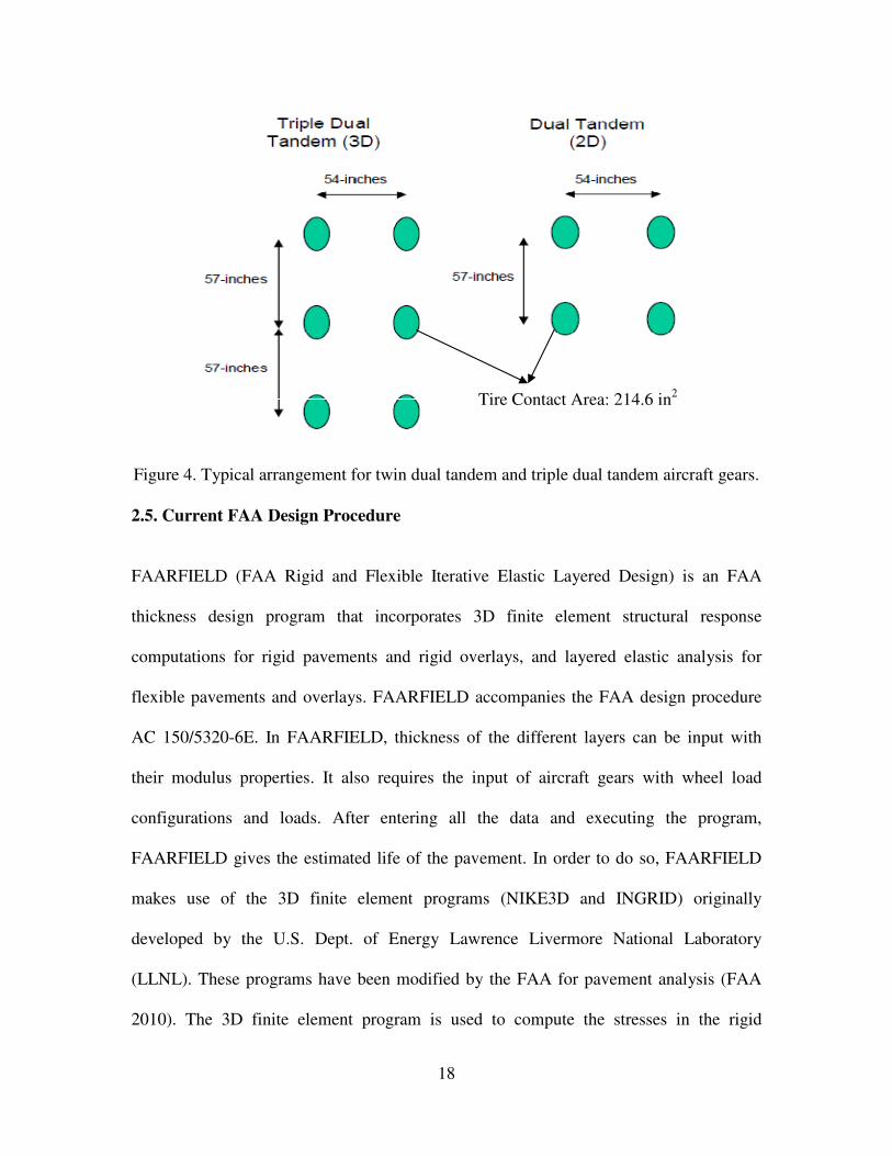
Figure 4. Typical arrangement for twin dual tandem and triple dual tandem aircraft gears.
Figure 5. Experimental design configuration, showing transverse joint spacings (Stoffels
et al., 2008).
Figure 6. End view of longitudinal joint locations for overlay and underlay slabs (Stoffels et
al., 2008).
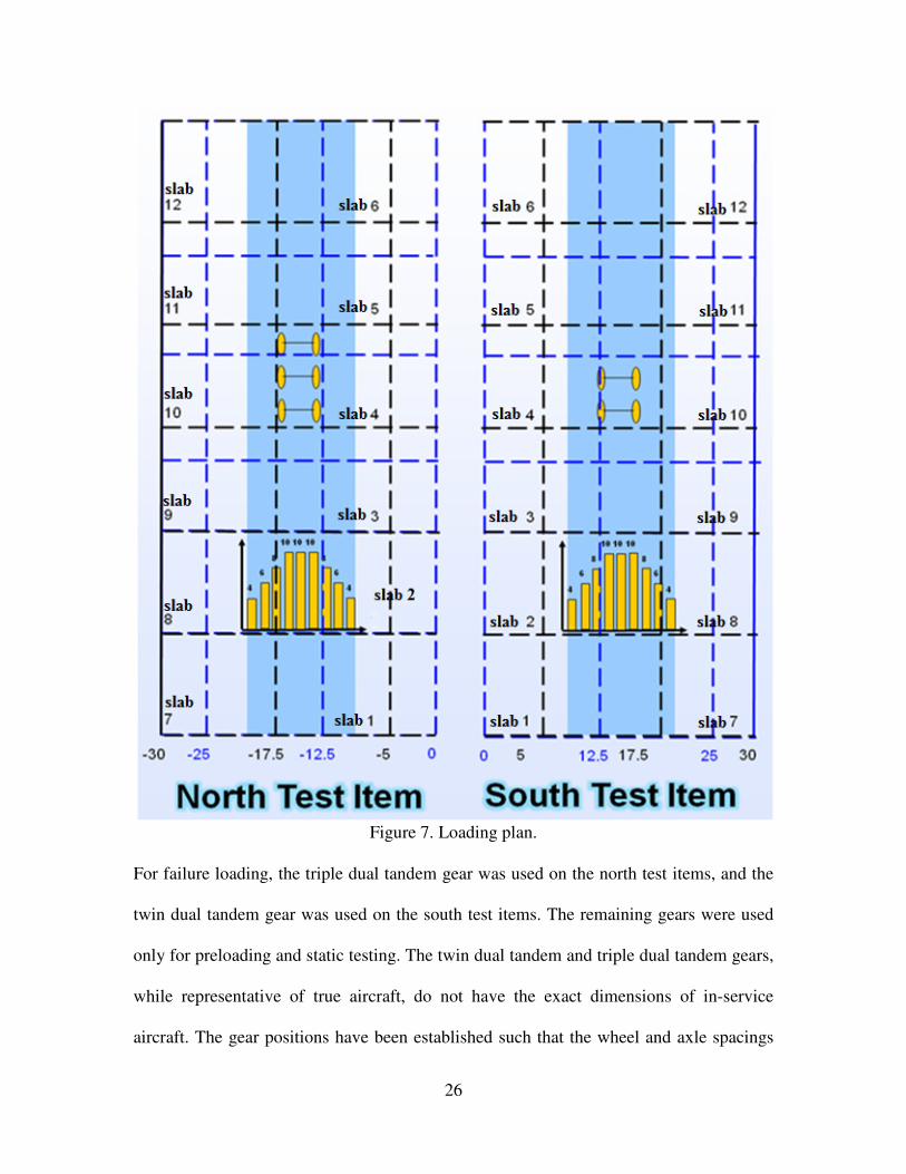
Figure 7. Loading plan.
Figure 8. Wander pattern and track frequencies (Stoffels et al., 2008).
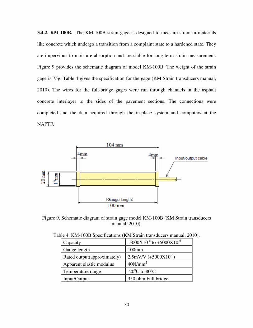
Figure 9. Schematic diagram of strain gage model KM-100B (KM Strain transducers manual,
2010).
Figure 10-a. Strain gage locations for a test item, longitudinal design view
Figure 10-b. Strain gage locations for a test item, transverse design view.
Figure 11.Expected peak strain condition for a mid-slab edge strain gage during loading.
Figure 12. Nomenclature for strain gage identification.
Figure 13-a. Strain gage instrumentation plan for the underlay of the pavement for test
items N1 and S1 (courtesy, prime contractor QES).
Figure 13-b. Strain gage instrumentation plan at the underlay of the pavement for test
items N2 and S2 (courtesy, prime contractor QES).
Figure 13-c. Strain gage instrumentation plan at the underlay of the pavement for test
items N3 and S3 (courtesy, prime contractor QES).

xiv
Figure 14-a. Strain gage instrumentation plan at the overlay of the pavement for test
items N1 and S1 (courtesy, prime contractor QES).
Figure 14-b. Strain Gage instrumentation plan at the overlay of the pavement for test
items N2 and S2 (courtesy, prime contractor QES).
Figure 14-c. Strain Gage instrumentation plan at the overlay of the pavement for test
items N3 and S3 (courtesy, prime contractor QES)
Figure 15. Flowchart of proposed methodology.
Figure 16. Flowchart of detailed process.
Figure 17. Strain gage average responses from one wander of ramp-up loading for gages
in test item north 1 with triple dual tandem loading (courtesy, Lin Yeh).
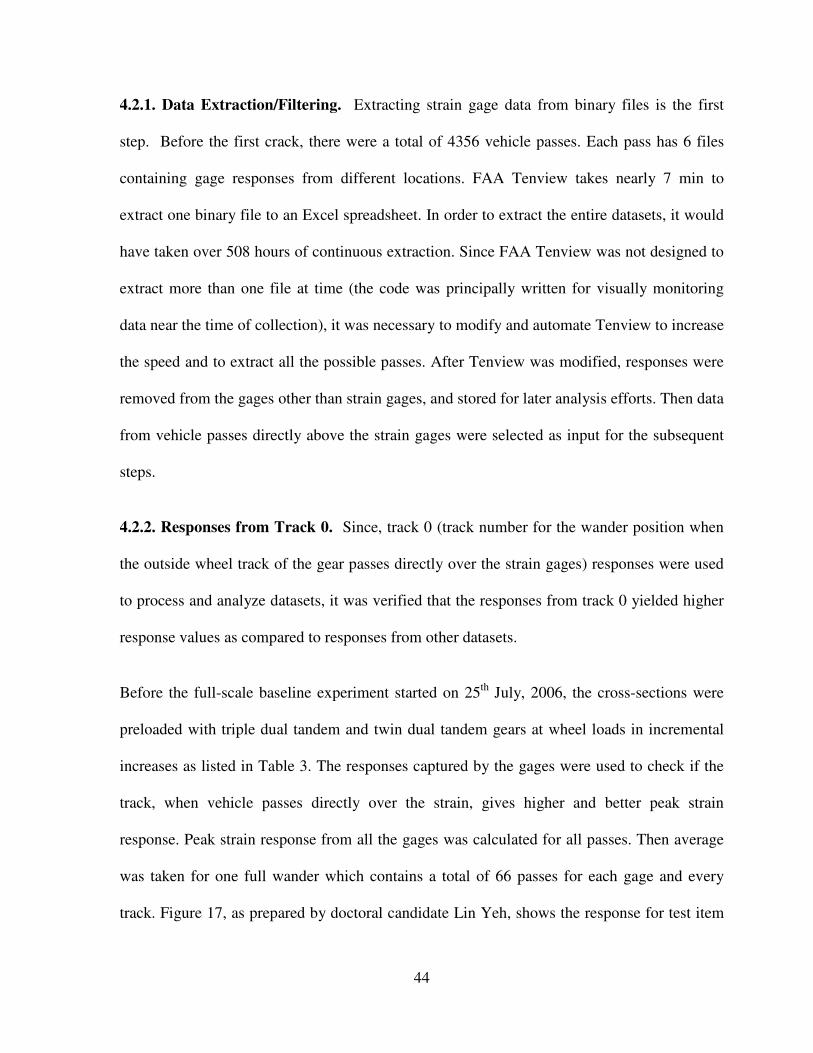
Figure 18. Baseline for a strain gage response.
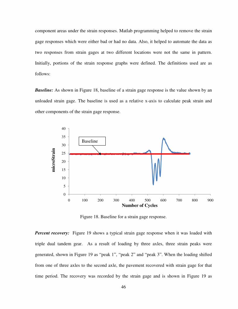
Figure 19. Peak strains and strain between axles for a strain gage response from triple
dual tandem loading.
Figure 20. Peak strains and strain between axles for a strain gage response from twin dual
tandem loading.
Figure 21. Cumulative area for a strain gage response from triple dual tandem loading.
Figure 22. Pre-stress area for a strain gage response from triple dual tandem loading.
Figure 23. Post-stress area for a strain gage response from triple dual tandem loading.
Figure 24. Duration for a strain gage response from triple dual tandem loading.
Figure 25. Strain gage response from triple dual tandem loading, type 1.
Figure 26. Strain gage response from triple dual tandem loading, type 2.
Figure 27. Strain gage response from triple dual tandem loading, type 3.
Figure 28. Strain gage response from triple dual tandem loading, type 4.
Figure 29. Strain gage response from twin dual tandem loading, type 1 and 2.
Figure 30. Strain gage response from twin dual tandem loading, type 3.

xv
Figure 31. Linear relationship between cumulative area and peak strain for EG-O-N1-1B.
Figure 32. Cumulative area plot for odd-numbered passes(west to east) for EG-O-N1-1B.
Figure 33. Peak strain plot for odd-numbered passes(west to east) for EG-O-N1-1B.
Figure 34. Cumulative area plot for even-numbered passes(east to west) for EG-O-N1-
1B.
Figure 35. Peak strain plot for even-numbered passes(east to west) EG-O-N1-1B.
Figure 36. Linear relationship between cumulative area and peak strain for EG-O-N1-1T.
Figure 37. Cumulative area plot for odd-numbered passes (west to east) for EG-O-N1-1T.
Figure 38. Peak strain plot for odd-numbered passes (west to east) for EG-O-N1-1T.
Figure 39. Cumulative area plot for even-numbered passes (east to west) for EG-O-N1-
1T.
Figure 40. Peak strain plot for even-numbered passes (east to west) for EG-O-N1-1T.
Figure 41. Gage locations used for analysis.

xvi
ACKNOWLEDGMENTS
I wish to thank all those who helped me. Without them, I could not have completed this
project. This thesis utilized data collected during previous research sponsored by the
FAA and the Innovative Pavement Research Foundation (IPRF). I would like to thank my
adviser, Dr Shelley Stoffels. Dr. Stoffels’ motivation and help kept me going through the
project. I would also like to thank Dr. Mansour Solaimanian, Dr Farshad Rajabipour and
Dr. Angelica Palomino for serving as members on my thesis committee and providing
assistance with my thesis. I would also like to acknowledge Lin Yeh, Nima Ostadi,
Dinesh Ayyala and Nitya Ramadoss for their support throughout my graduate career at
the Pennsylvania State University. Finally, I would like to thank the Federal Aviation
Administration (FAA), the Innovative Pavement Research Foundation (IPRF) and the
prime contractor for the full-scale testing project, Quality Engineering Solutions Inc.
(QES), for making this study possible.
1
CHAPTER 1. INTRODUCTION
1.1 Background
Aviation activity in the United States accounts for approximately forty percent of all
commercial aviation and fifty percent of all general aviation activity in the world (FAA,
2008). As a key industry in the United States, air transportation has a significant impact
on the economy. Air transportation faces the high cost of shutdowns due to rehabilitation
of airfield pavements, which also results in unnecessary delays to the traveling public.
Military airfields face similar problems when operational efficiency is affected by poor
pavement condition. Therefore, airfield pavements should be designed for better
performance and constructed with a high degree of quality (Kohn and Tayabji, 2003).
Concrete has been widely used in the construction of airport pavements because of its
durability and capacity to sustain large loads (Portland Cement Association, 2010).
Crack generation and propagation are among the most serious problems in concrete
pavements (Darestani, 2007; Hossain et al., 2003). Therefore, safe operation of aircrafts
requires airfield pavement condition assessment with timely performance of pavement
maintenance and repair (Greene et al., 2004). Pavement distress, structural capacity,
friction, and roughness are important factors for condition assessment (Greene et al.,
2004). Once the pavement condition is properly assessed, appropriate maintenance and
rehabilitation can be programmed and designed.
With the onset of a new generation of aircraft gears, including large multi-axled gears,
such as the triple dual tandem, airport pavement design assumptions need to be re-

2
examined to determine the potential effects of gear spacing and load levels on the
development of stresses and resulting fatigue life of concrete slabs (Roesler, Hiller, and
Littleton, 2004). Extensive research on stress development and fatigue of airport concrete
slabs has been performed, including the work from Westergaard (1926), the Lockbourne
and Sharonville test sections (Parker et al. 1979), the PCA design for airfields (Packard
1973, 1974), and the work by Rollings (1981, 1986, 1990, 1998, 2001) for the U.S. Army
Corps of Engineers (USACOE). Airfield concrete pavement fatigue has been extensively
studied by Smith and Roesler (2003) and Littleton (2003) (Roesler, Hiller, and Littleton,
2004).
Although portland cement concrete pavements have been used for the construction of
airfield pavements for many decades, and typically perform well, eventually all
pavements require rehabilitation or replacement. An unbonded concrete overlay offers an
attractive alternative for its use as an airfield pavement rehabilitation technique for
several reasons. Unbonded concrete refers to concrete pavement constructed over an
existing concrete pavement. The concrete layers are separated by an interlayer, typically
of hot-mix asphalt concrete, which acts as a shear zone, enabling the concrete layers to
move independently of each other. This is why the term unbonded is used (Pavement
Technology Advisory, 2005). One of the reasons unbonded concrete overlays are suitable
for airfield pavements is that, by leaving the existing pavement in place, the in situ
conditions of subgrade and base layers are essentially undisturbed, minimizing any
opportunity for additional consolidation or settlement to take place. Another advantage is
that the existing pavement can be taken into consideration in structural design, typically
resulting in a thinner and less costly required pavement layer (Stoffels et al., 2008),

3
which may be especially important for the heavy loads and thick pavement structures
typically required for airfields.
The Innovative Pavement Research Foundation (IPRF) has an objective of improving the
current understanding of the influence of design parameters on unbonded concrete
overlays of airfield pavements, thus enabling improvement of design methodologies and
consideration of the new aircraft. In 2005, IPRF contracted for a study to prioritize and
conduct the necessary research activities for the design of unbonded concrete overlays for
airfields, including a series of full-scale tests to be built at the Federal Aviation
Administration (FAA) National Airfield Pavement Test Facility (Stoffels et al., 2008).
The construction of the first of the IPRF unbonded overlays took place between
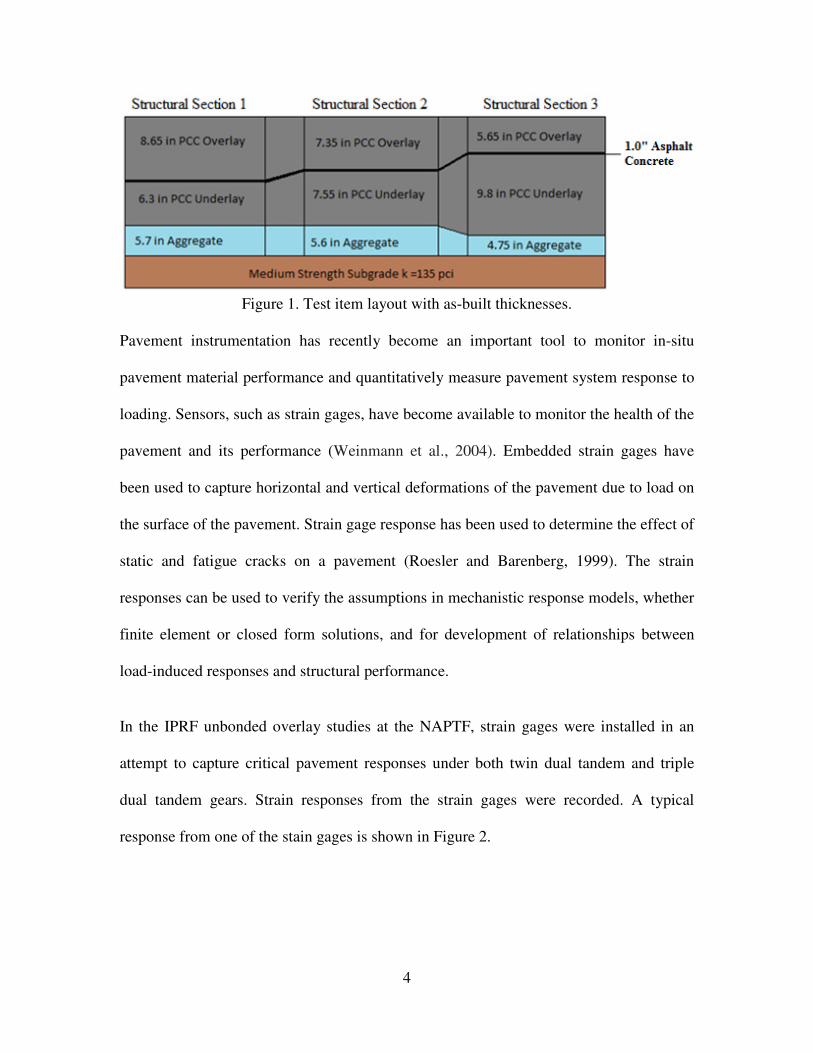
November 2005 and May 2006. Three 6000-ft2 pavement cross-sections, with thicker
overlay on thinner underlay, equal thicknesses of overlay and underlay, and thinner
overlay on thicker underlay, were built, as shown in Figure 1. The full-scale loading was
performed from July 2006 until November 2006 to study the effects of the relative
thickness of the overlay and underlay, the correspondence between predicted and
measured responses, the relative effects of two gear configurations, and the relationship
of the failure mechanisms in the existing pavement and overlay.
4
Figure 1. Test item layout with as-built thicknesses.
Pavement instrumentation has recently become an important tool to monitor in-situ
pavement material performance and quantitatively measure pavement system response to
loading. Sensors, such as strain gages, have become available to monitor the health of the
pavement and its performance (Weinmann et al., 2004). Embedded strain gages have
been used to capture horizontal and vertical deformations of the pavement due to load on
the surface of the pavement. Strain gage response has been used to determine the effect of
static and fatigue cracks on a pavement (Roesler and Barenberg, 1999). The strain
responses can be used to verify the assumptions in mechanistic response models, whether
finite element or closed form solutions, and for development of relationships between
load-induced responses and structural performance.
In the IPRF unbonded overlay studies at the NAPTF, strain gages were installed in an
attempt to capture critical pavement responses under both twin dual tandem and triple
dual tandem gears. Strain responses from the strain gages were recorded. A typical
response from one of the stain gages is shown in Figure 2.

5
Figure 2. Typical strain gage response as shown in FAA TenView.
Most of the previous studies on strain response in concrete pavements have focused on
the peak measured response from the strain gages, as defined in Figure 2. Peak strain
response has been used widely in different models to study the fatigue behavior and life
for the pavement. For this thesis, different components of strain response were analyzed
and compared to peak strain and to observed performance, to determine whether
additional valuable information can be extracted from the strain gage data. For example,
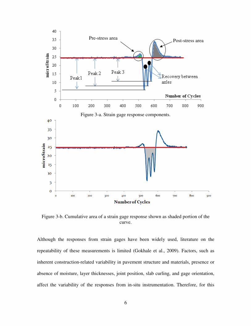
some of the components of strain gage response used are illustrated in Figure 3. Those
components include the peak values of strain for each axle of the gear, the recovery
between axles, the pre-stress and post-stress peaks, duration and the areas of the various
portions of the strain responses. Details of the strain response components are developed
and described in Chapter 4.
6
Figure 3-a. Strain gage response components.
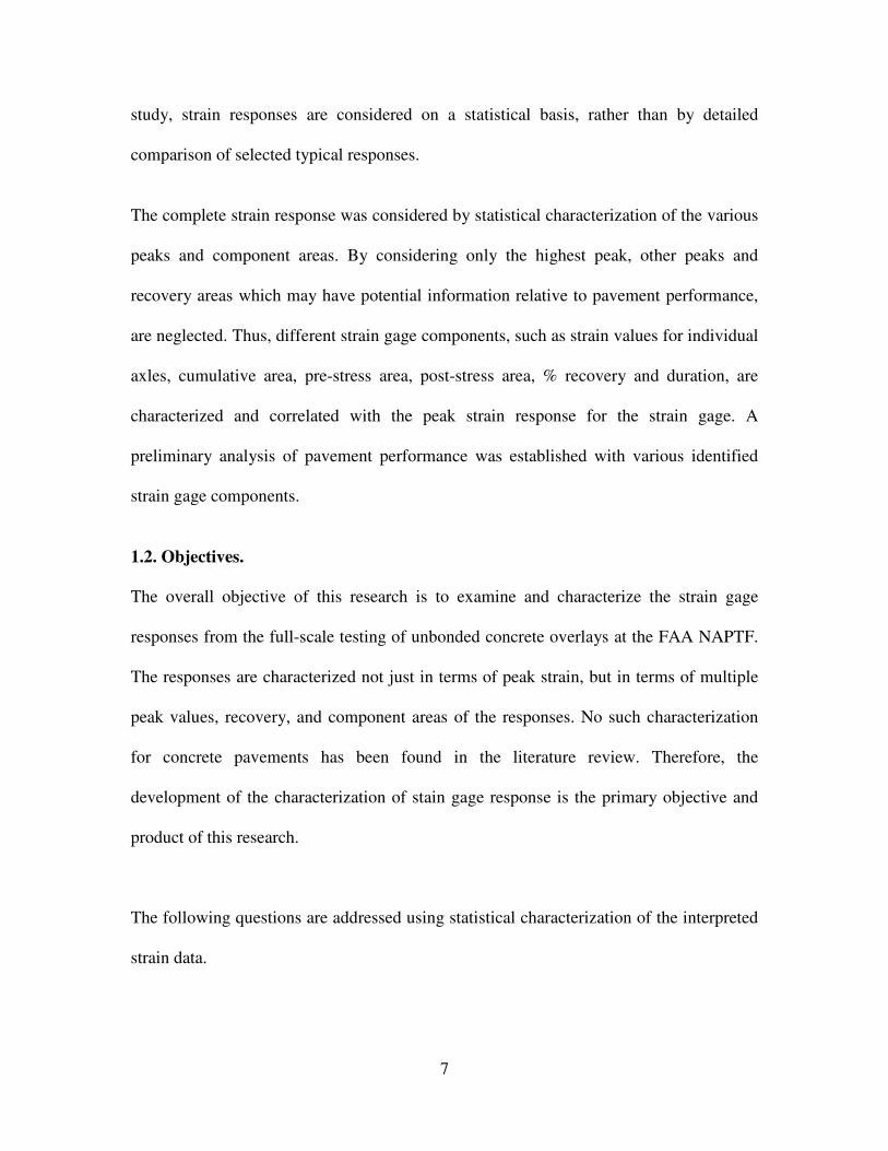
Figure 3-b. Cumulative area of a strain gage response shown as shaded portion of the
curve.
Although the responses from strain gages have been widely used, literature on the
repeatability of these measurements is limited (Gokhale et al., 2009). Factors, such as
inherent construction-related variability in pavement structure and materials, presence or
absence of moisture, layer thicknesses, joint position, slab curling, and gage orientation,
affect the variability of the responses from in-situ instrumentation. Therefore, for this
Pre-stress area Post-stress area
7
study, strain responses are considered on a statistical basis, rather than by detailed
comparison of selected typical responses.
The complete strain response was considered by statistical characterization of the various
peaks and component areas. By considering only the highest peak, other peaks and
recovery areas which may have potential information relative to pavement performance,
are neglected. Thus, different strain gage components, such as strain values for individual
axles, cumulative area, pre-stress area, post-stress area, % recovery and duration, are
characterized and correlated with the peak strain response for the strain gage. A
preliminary analysis of pavement performance was established with various identified
strain gage components.
1.2. Objectives.
The overall objective of this research is to examine and characterize the strain gage
responses from the full-scale testing of unbonded concrete overlays at the FAA NAPTF.
The responses are characterized not just in terms of peak strain, but in terms of multiple
peak values, recovery, and component areas of the responses. No such characterization
for concrete pavements has been found in the literature review. Therefore, the
development of the characterization of stain gage response is the primary objective and
product of this research.
The following questions are addressed using statistical characterization of the interpreted
strain data.
8
• Do the various components of the strain gage response, including peak strain
values for individual axles, cumulative area, pre-stress area, post-stress area,
percent recovery and duration, directly relate to the peak strain?
• How do the components of strain gage response change with different gear
configurations and different pavement cross-sections?
• If not directly related to peak strain, how do the components of the strain gage
response relate to observed performance in terms of cracking or structural
condition?
1.3. Scope
For this thesis, study is limited to analysis of the FAA NAPTF unbonded concrete
overlay strain gage data. Data before the first visually-observed crack was considered, as
these responses are most consistent and relate most directly to those that would be
predicted using a closed-form solution or finite element program for design purposes. For
the original study of the experiment, data was collected in different loading paths
consistent with the wander patterns on an airfield. The total number of loading passes
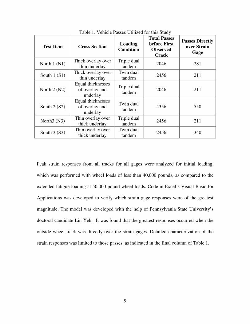
prior to the first observed crack for each test item is enumerated in Table 1. A test item is
defined as a unique combination of structural cross-section and gear configuration.
9
Table 1. Vehicle Passes Utilized for this Study
Test Item Cross Section Loading
Condition
Total Passes
before First
Observed
Crack
Passes Directly
over Strain
Gage
North 1 (N1) Thick overlay over
thin underlay
Triple dual
tandem 2046 281
South 1 (S1) Thick overlay over
thin underlay
Twin dual
tandem 2456 211
North 2 (N2)
Equal thicknesses
of overlay and
underlay
Triple dual
tandem 2046 211
South 2 (S2)
Equal thicknesses
of overlay and
underlay
Twin dual
tandem 4356 550
North3 (N3) Thin overlay over
thick underlay
Triple dual
tandem 2456 211
South 3 (S3) Thin overlay over
thick underlay
Twin dual
tandem 2456 340
Peak strain responses from all tracks for all gages were analyzed for initial loading,
which was performed with wheel loads of less than 40,000 pounds, as compared to the
extended fatigue loading at 50,000-pound wheel loads. Code in Excel’s Visual Basic for
Applications was developed to verify which strain gage responses were of the greatest
magnitude. The model was developed with the help of Pennsylvania State University’s
doctoral candidate Lin Yeh. It was found that the greatest responses occurred when the
outside wheel track was directly over the strain gages. Detailed characterization of the
strain responses was limited to those passes, as indicated in the final column of Table 1.
10
CHAPTER 2. LITERATURE REVIEW
2.1. Background.
Between 1927 and 1928, the first concrete airfield pavement was constructed at the Ford
Terminal, Dearborn, Michigan. Since then concrete pavements have been widely used at
both civilian and military airfields in the United States. The use of concrete for the
construction of runways, taxiways, and apron areas at airports has been popularized.
Naturally, there has been a great deal of evolution in the design and construction methods
applied to airport pavements. This evolution has been fueled by experience, field trials,
practice, and application of theoretical predictions (Kohn and Tayabji, 2003).
Furthermore, for many airfield applications, portland cement concrete is the preferred
material due to its much greater resistance to heat and fuel, in comparison to asphalt
concrete.
2.2 Concrete Properties.
Concrete properties such as concrete strength, modulus of elasticity, coefficient of
thermal expansion, shrinkage and concrete fatigue life play important roles to study the
possible fatigue failure mode of concrete pavements (Darestani, 2007). Tensile stresses at
the bottom of the concrete slab are generated by bending from the applied load on the
pavement. The load is transferred to sublayers by the bending action. In addition,
downward bending at slab corners or counter-flexure beyond the loaded area may induce
surface tensile stresses. Cracks on the top or bottom of the concrete surface are generated
when the flexural strength is exceeded by the stress induced by the applied load, or more
11
commonly from fatigue under repeated loading. Cracks propagate into the depth of the
concrete slab from the surface of the pavement, or vice versa. This is one of the main
reasons behind concrete deterioration, and thus flexural strength or modulus of rupture is
considered a major concrete property. Flexural Strength plays an important role in
concrete pavement design guides (Darestani, 2007), and in construction material
specifications for airfields.
Modulus of elasticity is a property of the concrete which reflects the stiffness of concrete
under static load. For a concrete of a given strength, Neville (1996) pointed that a higher
aggregate content results in higher modulus of elasticity of the concrete because normal
weight aggregate had a higher elastic modulus than hydrated cement paste (Tia et al.,
2005). Modulus of elasticity is dependent on the concrete materials and mix proportions
(ACI, 1992; Darestani, 2007). Thermal coefficient of the concrete depends on the
concrete constituents and moisture contents (Neville, 1983). Concrete’s coefficient of
thermal expansion is dependent on the coefficient of thermal expansion of cement paste
and aggregates. Cement paste has a coefficient of thermal expansion between 11×10-6
and 20×10-6
mm/mm/°C which is greater than aggregate thermal expansion coefficient
(Meyers, 1951). The type and percentage of aggregates in a concrete mix, associated with
curing method, can affect the magnitude of coefficient of thermal expansion in concrete
as thermal movement of the cement paste is restrained by aggregates (Darestani, 2007).
Three types of concrete shrinkage have been identified, namely, plastic shrinkage, drying
shrinkage, and carbonation shrinkage (Nawy, 2001). Plastic shrinkage happens during the
first hours after placing fresh concrete in the forms. It is affected by the ratio of the

12
surface area to the thickness of the concrete elements. Drying shrinkage, on the other
hand, occurs during the final setting of concrete when the cement hydration process is
nearing its completion. It is a decrease in the volume of the concrete element due to the
evaporation of moisture. Reaction between carbon dioxide (CO2) in the atmosphere and
calcium hydroxide in the cement paste causes carbonation shrinkage (Nawy, 2001;
Darestani, 2007). Shrinkage cracking may play a role in the initiation of subsequent load-
related cracking.
2.3. Concrete Pavement Fatigue.
Fatigue is failure of structural elements due to repeated loads, when the magnitude of
applied load is not large enough to cause immediate failure in the elements. Repeated
loads such as cyclic loads result in fatigue failure of the concrete under a load less than its
flexural strength (Karimov, 2004; Darestani, 2007). The maximum stress experienced by
the concrete during loading has been widely studied to define fatigue. A number of such
models for concrete fatigue have been developed.
2.3.1. Stress Ratio Models. Stress ratio (SR) has been defined as the ratio of the
maximum tensile bending stress experienced by the concrete slab to the concrete modulus
of rupture. Rao (2004) also described several fatigue curves for concrete pavement,
which have been developed using field and laboratory data that relate the stress ratio to
the number of loads until failure. These include the following (Rao et al., 2004).
1) Zero-Maintenance Design Beam Fatigue Model (Darter et al., 1976, 1977) ―
Concrete beams were used to develop this model. Complete beam fracture was taken as

13
the failure criterion. Bending beam equations were used to calculate the load stresses at
the bottom of the beam.
log Nf = 17.61 – 17.61 SR (1)
Where, Nf = Number of stress applications to failure for the given stress ratio SR.
2) Calibrated Mechanistic Design Field Fatigue Model (Salsilli et al., 1993). This
was developed using Corp of Engineers (COE) field aircraft data and American
Association of State Highway Officials (AASHO) Road Test data. Fifty percent slab
cracking was taken as the failure criteria in this method. The finite element program,
“ILLI-SLAB” was used to calculate load and temperature curling stresses at the edge.
log � = ����. ����� (���)�.���� �
�.���� (2)
Where, P = Cracking probability.
3) ERES/COE Field Fatigue Model (Darter, 1988). This model was also developed
using Corp of Engineers (COE) field aircraft data. Similar to the Calibrated Mechanistic
Design Field Fatigue Model, the failure criterion was defined as fifty percent slab
cracking. Instead of ILLI SLAB as used in Calibrated Mechanistic Design Field Fatigue
Model, influence chart software, known as H-51 (Rao et al., 2004), was used to find
stress at the slab edge. In order to account for load transfer and support conditions, stress
was reduced by a factor of 0.75.
log N = 2.13 SR-1.2
(3)

14
4) Foxworthy Field Fatigue Model (Foxworthy 1985). This model is similar to
Calibrated Mechanistic Design Field Fatigue Model. It was developed using Corp of
Engineers (COE) field aircraft data. Similar to the Calibrated Mechanistic Design Field
Fatigue Model, the failure criterion was defined as fifty percent slab cracking. ILLI
SLAB was used to find load stress at the slab edge.
log � = 1.323 ! ��" + 0.588 (4)
5) PCA Beam Fatigue Model (Packard et al., 1983) ― This model is similar to the
Zero-Maintenance Design Beam Fatigue Model. Concrete beams were used to develop
this model. Complete beam fracture was taken as the failure criterion. Bending beam
equations were used to calculate the load stresses at the bottom of the beam.
log N = 11.737 - 12.077 SR for SR ≥0.55 (5)
N= � '.�(��)*��.'��(�
�.��+for 0.45 < SR < 0.55 (6)
N = unlimited for SR ≤0.45.
2.3.2. Slab Fatigue. Fatigue curves for beams always show lesser resistance to the
cracking as compared to fatigue curves as predicted for slabs (Roesler, 2006). Therefore,
fatigue curves for slabs cannot be predicted from beam fatigue curves, and this has been
confirmed by full scale testing on concrete slabs (Roesler et al., 1998, 2004, 2005).
Gaedicke (2009) studied a fracture-based method to predict the fatigue crack growth of
small-scale specimens which is extended to predict the crack growth in concrete slabs
supported by a soil foundation. Gaedicke (2009) developed fatigue model in which
concrete slabs were tested in the cyclic loading at the same level. This methodology

15
allows for the future prediction of the remaining fatigue life of new and partially-cracked
concrete slabs for a variety of pavement applications (Gaedicke et al., 2009).
2.3.3 Variable Amplitude Loading. Highways and airport pavements are subjected to
millions of cycles of repeated axle loads. Repetitive loading tends to deteriorate both
stiffness and the strength of the concrete as a result of accumulated damage (Yun et al.,
2005). Since most of the studies are based on constant amplitude loading instead of
variable amplitude loading, Yun (2005) studied accumulated damage and methods of
concrete testing under variable loading. Yun (2005) adopted the linear damage theory by
Miner, 1945 (Yun et al., 2005), nonlinear theory proposed by Oh, 1991 (Yun et al., 2005)
and the equivalent damage theory proposed by Marin (Yun et al., 2005). Yun (2005)
found that split tensile test results were equivalent to or better than the flexural tensile test
results for application to the equivalent damage theory. Thus, remaining life of concrete
under fatigue damage could be predicted by splitting tensile test (Yun et al., 2005).
2.3.4 Mechanistic Approach. Hiller and Roesler (2005) developed a mechanistic
approach in conjunction with Miner’s Hypothesis to calculate fatigue damage for
California rigid pavements. Hiller and Roesler (2005) predicted the location and
magnitude of concrete damage by using concrete fatigue transfer functions accounting for
stress range or maximum stress. It was observed that factors such as effective built-in
temperature difference, steer-drive axle spacing, load transfer level, lateral wheel wander
distribution, and climatic region controlled critical damage location and magnitude. Top-
down and bottom-up transverse, longitudinal, and corner cracking occurred in the slabs
with curling (Hiller and Roesler, 2005).
16
2.3.5 Numerical Approach (Finite-Element Methods). Kuo et al. (2004) investigated
the effects of impact load by landing of heavy aircrafts in which “the angle of landing by
a single-wheel impact load is greater than the static load for the same aircraft, with
inclusion of the effects of the shock-absorption system” on the runways. From the
numerical model calculated by Kuo et al. (2004), theoretical stresses and strains that were
computed by existing elastic-layer and finite-element computer programs indicated that
tensile strength is ten times more than that of static loading for the base of asphalt layer
and compression strains at the top of the subgrade (Kuo et al., 2004).
2.3.6 Fuzzy Logic. Tigdemir (2002) used fuzzy logic for estimating fatigue life from
deformation measurement by employing theory of fuzzy sets and by representing fatigue
life and deformation relations as a set of fuzzy rules. Fatigue life and deformation are
intimately related phenomena and a model involving a relationship between them can
best be derived by methods that explicitly take vagueness into account (Tigdemir et al.,
2002).
2.4. Airbus A-380 and Boeing 777
With local and regional aviation going through rapid changes, airline companies are
trying to improve their efficiency in order to remain profitable. Therefore, introduction of
supersized aircrafts like the new Airbus aircraft has been welcomed by many in the
aviation industry. But the introduction of new super-sized aircrafts has been challenging
to the civil engineering profession. Different landing gear configurations, in different
aircraft such as the Boeing 777 and the Airbus A-380, also affect the assumptions by
which engineers design the airport pavements (Khoon and Meng, 2005). Thus, loading

17
type and repetition have been important to a civil engineer in the fatigue study of airfield
pavements. Loading due to operation of a particular aircraft is dependent on the number
of the aircraft passes, the number and the spacing of the wheels on the aircraft main
landing gear, the width of tire-contact area, and the lateral distribution of the aircraft
wheel-paths relative to pavement centerline or guideline marks (HoSang, 1975).
Design and evaluation of an aircraft pavement has been based on the theoretical analysis
of the structural thickness coupled with full-scale tests on in-service pavements. The most
important considerations in the design methods are the gear and wheel arrangements
(Khoon and Meng, 2005). Previous design guides given by FAA made assumptions with
respects to wheel and gear configurations such as single wheel gear, dual wheel gear,
dual tandem gear and also specific charts for wide body aircrafts with double dual tandem
gears such as A-300 and B747. However, gear and wheel arrangement of Airbus A-380
and Boeing 777 with its triple dual tandem main gear are different when compared to
existing super-sized aircraft with twin dual tandem main gears. Triple dual tandem is
unique, with six wheels in the aircraft arranged as three pairs of wheels in a row. Figure 4
shows the arrangement for twin dual gear and triple dual gear for an aircraft. The
spacings vary between aircraft, and these spacings are not exactly representative of any
specific aircraft. They are, however, the exact gear configurations used during the full-
scale testing of unbonded overlays at the NAPTF.
18
Figure 4. Typical arrangement for twin dual tandem and triple dual tandem aircraft gears.
2.5. Current FAA Design Procedure
FAARFIELD (FAA Rigid and Flexible Iterative Elastic Layered Design) is an FAA
thickness design program that incorporates 3D finite element structural response
computations for rigid pavements and rigid overlays, and layered elastic analysis for
flexible pavements and overlays. FAARFIELD accompanies the FAA design procedure
AC 150/5320-6E. In FAARFIELD, thickness of the different layers can be input with
their modulus properties. It also requires the input of aircraft gears with wheel load
configurations and loads. After entering all the data and executing the program,
FAARFIELD gives the estimated life of the pavement. In order to do so, FAARFIELD
makes use of the 3D finite element programs (NIKE3D and INGRID) originally
developed by the U.S. Dept. of Energy Lawrence Livermore National Laboratory
(LLNL). These programs have been modified by the FAA for pavement analysis (FAA
2010). The 3D finite element program is used to compute the stresses in the rigid
Tire Contact Area: 214.6 in2
19
pavements and rigid overlays. During execution, FAARFIELD fetches the peak strain in
order to calculate the estimated life of the pavement.
2.6 Structural Condition Index
Rollings (1988) developed the Structural Condition Index (SCI) based on visual surveys
of the pavement condition. SCI is defined as a function of the number, width and type of
structural distresses in a pavement. SCI is derived from the distress definitions and deduct
values as determined by ASTM D 5340 Airport Pavement Condition Index Surveys
(Rollings, 1988). The Pavement Condition Index (PCI) is a numerical indicator that rates
the surface condition of the pavement. An objective and rational basis for determining
priorities and maintenance and repair needs is provided by the PCI (Standard Test
Method for Airport Pavement Condition Index Surveys, 2004). SCI is the component of
the PCI which addresses structural damage.
2.7. Strain Gage Characterization
There have been very few attempts to characterize strain gage response components such
as cumulative area, pre-stress area, post-stress area, % recovery and duration. Chou and
Wang (2005) analyzed data recorded by H-bar strain gauges, which were installed at
various depths of concrete pavement, generated by the taxing aircraft, including the
variation of strain induced by aircraft of different gear configurations. They concluded
that by looking at strain gage response, the main gear configuration of an aircraft can be
identified with a number of peaks. They also added that the time point when the peak
strain happened could be used to figure out the location of the loading.
20
Guo et al. (2002) studied the strain gage responses from three types of portland cement
concrete pavements, built at the Federal Aviation Administration’s (FAA) National
Airport Pavement Test Facility (NAPTF) in 2000, with traffic loads consisting of four-
and six-wheel carriages at 45,000 lbs. Though the data from 462 strain gages was
recorded during testing, Guo et al. (2002) could only study a small portion of the data.
Peak strain responses from all the axles in a gear configuration were studied to analyze
the corner crack in the pavement. They concluded that the measured strain gage
responses contain significant information which can help understand slab behavior under
simulated aircraft traffic loading.
It is evident that in these prior studies, peak strain has been widely investigated regarding
its effect on pavement structural responses and fatigue performance. Peak strain is
typically used because it defines the maximum stress developed during the course of
loading, which is considered as a critical component affecting the pavement life. . In
addition, with the assumptions needed for traditional closed-form solutions for concrete
slab analysis, results were often inherently limited to maximum values (Westergaard,
1948; Ioannides, 1985).
2.8. Summary of Important Findings from Literature Review
It can be summarized from the above literature that current procedures to develop
different fatigue models principally utilize the maximum peak strain response from
application of a gear load. There has been no or minimal attempt to consider the
accumulated peak responses from different gear configurations, the recovery between
axles, or the total strain amplitudes. Different types of models have been developed

21
including mechanistic approaches and different numerical approaches such as fuzzy logic
and finite element methods. All the models found during this literature review use peak
strain response, irrespective of the different gear configuration or different pavement
cross section. The FAA has upgraded FAARFIELD extensively to match the new gear
configuration and its impact on the calculation on the life of the pavement, and has made
the computer program part of the design procedure, as opposed to reliance on design
charts. FAARFIELD also relies on the peak strain response as the important factor in the
calculation of pavement estimated life, which may or may not be appropriate for all gear
configurations. FAARFIELD, however, is calibrated by the results of past field and
accelerated tests and performance observations.

22
CHAPTER 3. FULL-SCALE TESTING OF UNBONDED OVERLAYS
The Innovative Pavement Research Foundation (IPRF), in cooperation with the FAA,
with an objective of improving the current design methodology and understanding of the
influence of design parameters for airfield unbonded concrete overlays, initiated full-
scale testing at the NAPTF. Three different thickness concrete airport pavement sections
were constructed over the same subgrade with medium support. The sensor installation
included strain gages, linear position transducers and pressure cells to capture critical
pavement responses under twin dual tandem and triple dual tandem gears. The prime
contractor was Quality Engineering Solutions Inc. (QES). The Baseline Experiment was
initiated in September 2005 and the SCI Validation Study began in 2007. These results
serve to help in the future validation/calibration of concrete pavement structural response
models, and, hence, aid in the development of better tools for the design/evaluation of
airport pavement systems.
3.1. NAPTF
The FAA operates a state-of-the-art, full-scale pavement test facility dedicated solely to
airport pavement research which was constructed in April 1999. The National Airport
Pavement Test Facility (NAPTF) is located at the William J. Hughes Technical Center
near Atlantic City, New Jersey. High quality, accelerated test data from rigid and flexible
pavements are acquired at the facility by simulating aircraft traffic. NAPTF has a fully
enclosed instrumented test track, computerized data acquisition system, controlled
aircraft wander simulation, a test vehicle capable of simulating aircraft weighing up to
1.3 million pounds, wheel loads independently adjustable up to 75,000 pounds per wheel
23
and up to 20 test wheels capable of being configured to represent two complete landing
gears (FAA 2010).
3.2. Pavement Cross-Sections
An approximately 300-foot test pavement was constructed as a baseline experiment at
FAA’s testing facility. It was constructed on the medium subgrade, and had three
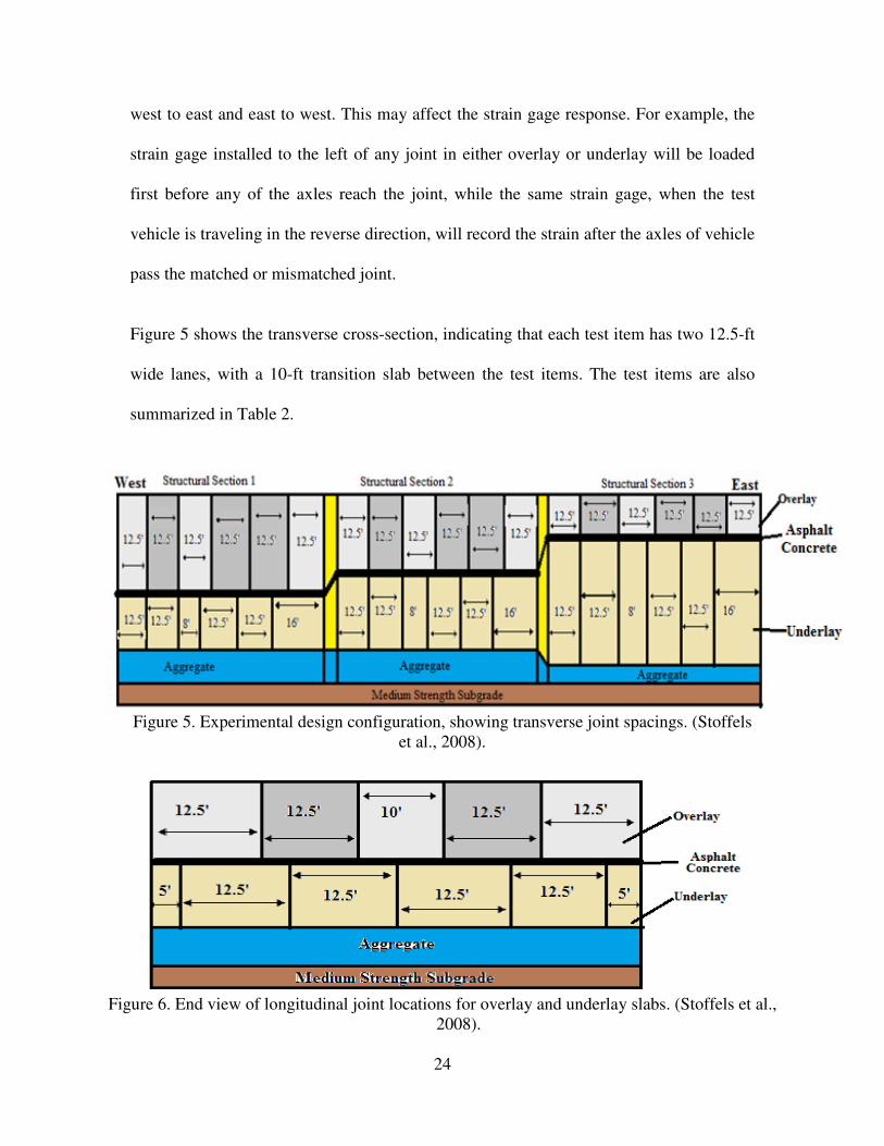
structural cross-sections as shown in Figures 5 and 6 (Stoffels et al., 2008). The
underlying slabs were not designed to be distressed (no shattered or cracked slabs), but to
have different joint matching conditions to determine how underlying discontinuities
(including cracks) affect the overlay’s performance. Having an intact underlay also
allows investigation of deterioration of the underlying pavement due to overlay loading
(Stoffels et al., 2008).
Thus, the final design for the Baseline Experiment consisted of six test items of 12 slabs
each. The test items were separated by transition slabs in both the longitudinal and
transverse directions. By providing two test items in each structural section, different
loading configurations could be applied. Figure 5 shows the three structural cross-
sections, numbered 1, 2 and 3 from west to east. Numbers in Figure 5 and Figure 6
indicate the width of the slabs in feet. Joint patterns were established to create matched
and mismatched joints in the underlying slab and the concrete overlay as shown in
Figures 5 and 6. All longitudinal joints are mismatched or offset as shown in Figure 6.
The transverse joints have some matched and some offset as shown in Figure 5. The
underlay joints were sawcut and not doweled. All overlay joints, both transverse and
longitudinal, were doweled and sawcut. The structural cross-section was loaded from
24
west to east and east to west. This may affect the strain gage response. For example, the
strain gage installed to the left of any joint in either overlay or underlay will be loaded
first before any of the axles reach the joint, while the same strain gage, when the test
vehicle is traveling in the reverse direction, will record the strain after the axles of vehicle
pass the matched or mismatched joint.
Figure 5 shows the transverse cross-section, indicating that each test item has two 12.5-ft
wide lanes, with a 10-ft transition slab between the test items. The test items are also
summarized in Table 2.
Figure 5. Experimental design configuration, showing transverse joint spacings. (Stoffels
et al., 2008).
Figure 6. End view of longitudinal joint locations for overlay and underlay slabs. (Stoffels et al.,
2008).

25
Table 2. Summary of Design Test Items for Baseline Experiment
Test Item
Designation
As-Built
Overlay
Thickness
(in)
As-Built
Underlay
Thickness
(in)
Nominal
Interlayer
Thickness
(in)
Planned Gear
Loading
North 1 (N1) 8.65 6.30 1.00 Triple Dual Tandem
South 1 (S1) 8.65 6.30 1.00 Twin Dual Tandem
North 2 (N2) 7.35 7.55 1.00 Triple Dual Tandem
South 2 (S2) 7.35 7.55 1.00 Twin Dual Tandem
North 3 (N3) 5.65 9.80 1.00 Triple Dual Tandem
South 3 (S3) 5.65 9.80 1.00 Twin Dual Tandem
3.3. Types of Loading and Aircraft Gears.
The NAPTF test vehicle has two carriages, which can be used for loading simultaneously
or independently. Each carriage also has flexibility in the choice of gear configuration,
the selection of wheel load level, and in carriage position. During loading, the FAA
personnel at the NAPTF monitored the control of the wheel load level and carriage
position. The wheel load levels were within control throughout the experiment, and thus
only the target wheel loads are reported here. Tire pressures were also monitored, with an
unloaded inflation pressure of 233 psi. The use of a constant inflation pressure means that
contact areas vary with load level. The test speed was three miles per hour. The gear
configurations used at the NAPTF during this experiment are illustrated in Figure 4 and
Figure 7.
26
Figure 7. Loading plan.
For failure loading, the triple dual tandem gear was used on the north test items, and the
twin dual tandem gear was used on the south test items. The remaining gears were used
only for preloading and static testing. The twin dual tandem and triple dual tandem gears,
while representative of true aircraft, do not have the exact dimensions of in-service
aircraft. The gear positions have been established such that the wheel and axle spacings
27
are the same for all configurations. The dual wheels are spaced at 54 inches center-to-
center. The spacing between axles is 57 inches, as illustrated in Figure 4.
The transverse position of the carriages was shifted between passes to simulate vehicle
wander. A wander pattern consisted of 66 passes, with each passage of the test vehicle to
the east being counted as a pass, and the return to the west counting as a second pass. The
carriage completed the two-pass down and back cycle before being shifted. A wander
pattern consisting of nine carriage (gear) positions, each shifted by 10.25 inches, was
used for all dynamic loading with the test vehicle. This wander pattern was previously
used by the FAA at the NAPTF, and was determined to be a reasonable estimation of real
airfield wander patterns. By using the same pattern, the ability to compare failure data
across construction and testing cycles at the NAPTF is also improved. The standard
wander pattern and track frequencies are shown in Figure 8.
Test vehicle loading of the test items occurred in a number of stages. The dates and wheel
loads for each stage of loading are summarized in Table 3. The number of wanders and
dates for the failure loading varied by test item. During the loading, when the direction
was from west to east, the data was recorded as odd-numbered passes. Then the load was
returned from east to west and recorded as even-numbered passes.

28
Figure 8. Wander pattern and track frequencies. (Stoffels et al., 2008).
Table 3. Loading Sequences (Stoffels et al., 2008)
Dates Wanders Wheel Loads
(lbs) Purpose
3/14/2006 44 passes 10000 Seating Load on Underlay
3/14/2006 to 3/15/2006 4 15000 Gear Response Loading on
Underlay
3/15/2006 NA 10000 Static Loading on Underlay
5/22/2006 to 5/23/2006 88 passes 10000 Seating Load on Overlay
5/23/2006 NA 15000 Static Loading on Overlay
5/23/2006 to5/24/2006 4 20000 Gear Response Loading on
Overlay
7/6/2006 NA 20000 Interaction Loading
7/6/2006 to7/12/2006
1
2
3
20000
30000
40000
Ramp-Up Loading
7/25/2006 to10/31/2006 Varied 50000 Failure Loading
29
3.4. Instrumentation.
3.4.1. Strain Gages. Although other instrumentation was utilized for the full-scale
testing, this thesis study focused exclusively on the strain gage responses. Strain gages
were used to measure the strain near the top and bottom of the slab. The frequency at
which the strain gage response was captured was 20 Hz. The number of data samples for
a stain gage ranged between 700 to 1000 for one pass of loading, thus data captured for a
strain gage response has a total duration of 35 seconds to 50 seconds. For this study,
strain gage model KM-100B by manufacturer Tokyo Sokki Kenkyujo was used.
A pair of embedded strain gages was installed at each location to measure strain near the
top and bottom of the slab in the longitudinal direction of the pavement. These gages
were usually located at the mid slab (transverse center of the slab) of the loaded joint.
Embedded strain gages were installed during the paving operation. During the slab
construction, the cans were used to install the strain gages in the pavement. These
instrumentation cans were carefully hand filled with concrete completely encasing the
strain gages. Next, concrete was piled around the cans to hold them in place. In order to
keep the instrumentation wiring out of the underlying slabs, trenches were dug in the base
course and wires placed within them. Prior to placement of the underlying slab, these
trenches were backfilled with concrete sand and compacted using hand tampers. Rebar
chairs were used to make certain the top gages were set at the proper height, one inch
below the top surface of the pavement layer. A spacer was used to make sure that the
bottom gage was completely covered by concrete and any part of the gage could not rub
against the surface of the substrate layer when the slab moves (Stoffels et al., 2008).
30
3.4.2. KM-100B. The KM-100B strain gage is designed to measure strain in materials
like concrete which undergo a transition from a complaint state to a hardened state. They
are impervious to moisture absorption and are stable for long-term strain measurement.
Figure 9 provides the schematic diagram of model KM-100B. The weight of the strain
gage is 75g. Table 4 gives the specification for the gage (KM Strain transducers manual,
2010). The wires for the full-bridge gages were run through channels in the asphalt
concrete interlayer to the sides of the pavement sections. The connections were
completed and the data acquired through the in-place system and computers at the
NAPTF.
Figure 9. Schematic diagram of strain gage model KM-100B (KM Strain transducers
manual, 2010).
Table 4. KM-100B Specifications (KM Strain transducers manual, 2010).
Capacity -5000X10-6
to +5000X10-6
Gauge length 100mm
Rated output(approximately) 2.5mV/V (+5000X10-6
)
Apparent elastic modulus 40N/mm2
Temperature range -20oC to 80
oC
Input/Output 350 ohm Full bridge

31
Strain generated in the specimen is transmitted to the gage (foil or wire resistor) when
expansion or contraction occurs. As a result, the resistor experiences a change in
resistance. This change is proportional to the strain as indicated in the following equation
Strain= Calibration Factor ∗ 2 ∗ ∆eE (7)
Where, ∆e:Voltage output; E:Exciting voltage(input voltage=5V),
Calibration factors for all strain gages are included in Appendix A.
For the baseline unbonded concrete overlay experiment, strain gages were installed in the
longitudinal direction of the pavement, placed in-situ near the top of the unbonded
overlay, the bottom of the overlay, the top of the underlay and the bottom of the underlay.
There were two additional strain gages installed at the top and bottom of underlay for test
item 2, as shown in Figure 10. Figure 10 shows the instrument locations relative to the
transverse and longitudinal end views of the pavement sections.
Figure 10-a. Strain gage locations for a test item, longitudinal design view.
asphalt

32
Figure 10-b. Strain gage locations for a test item, transverse design view.
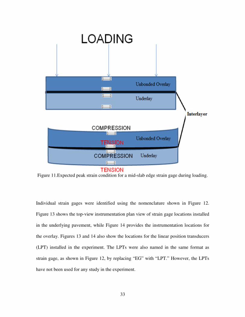
Figure 11 shows a schematic diagram of the concrete slab of unbonded overlay over
underlay. When the surface of the overlay is loaded, the top of the overlay and the top of
the underlay go into compression, and the bottom of the overlay and the bottom of the
underlay go into tension. Due to the compression and tension, resistance of a strain gage
installed at top and bottom of overlay and underlay, shown in Figure 11, changed and
output voltage was recorded for the change in resistance. The output voltage was later
converted to engineering units by using equation 7. Appendix A gives the coordinates for
each strain gage.
Asphalt
concrete
33
Figure 11.Expected peak strain condition for a mid-slab edge strain gage during loading.
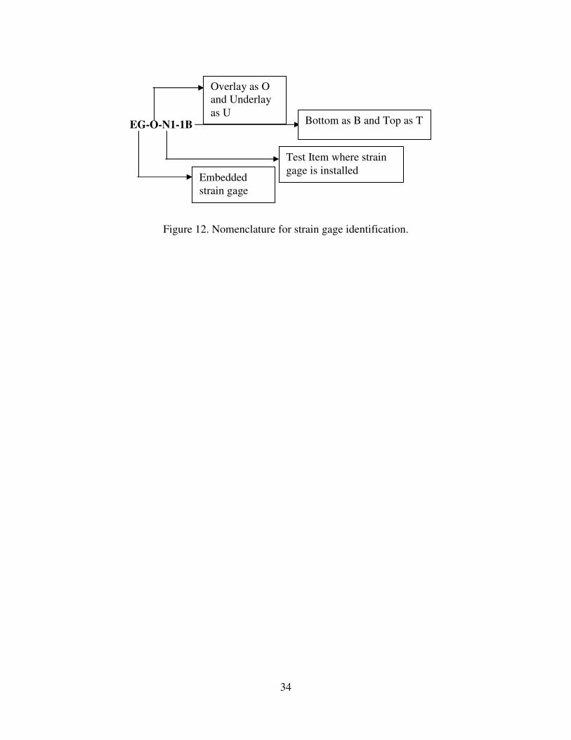
Individual strain gages were identified using the nomenclature shown in Figure 12.
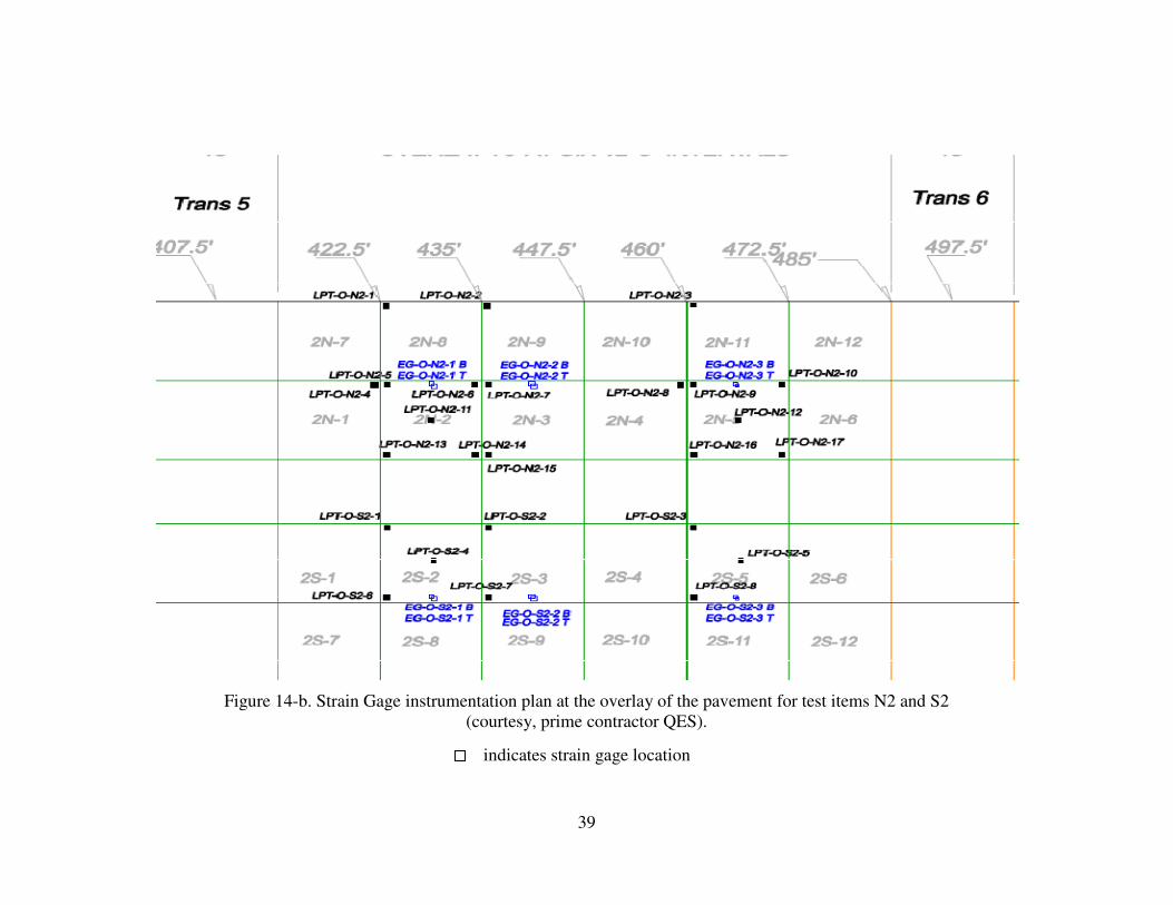
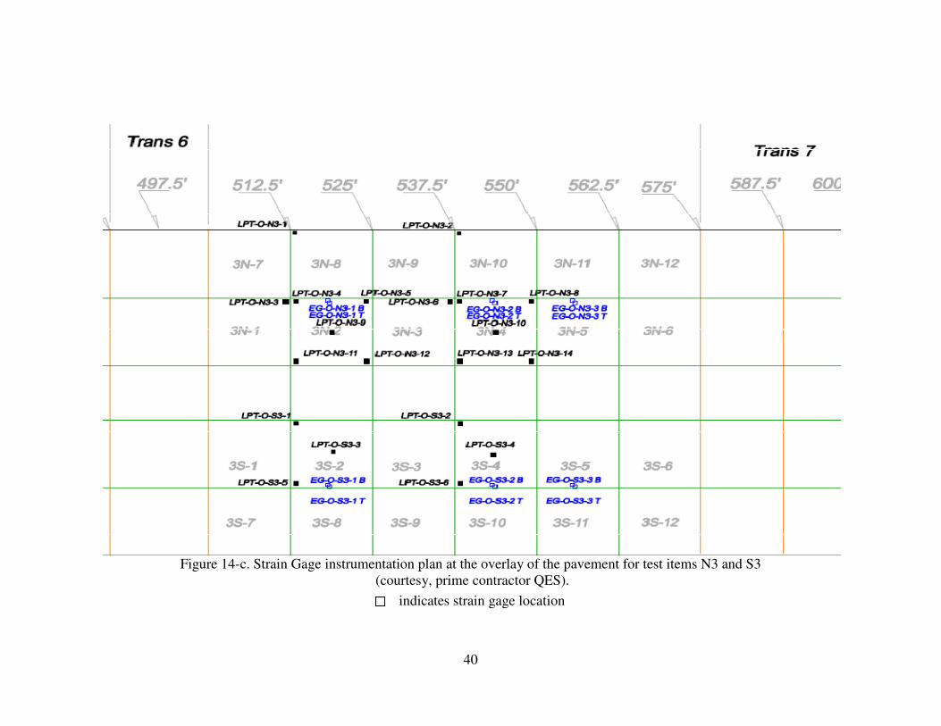
Figure 13 shows the top-view instrumentation plan view of strain gage locations installed
in the underlying pavement, while Figure 14 provides the instrumentation locations for
the overlay. Figures 13 and 14 also show the locations for the linear position transducers
(LPT) installed in the experiment. The LPTs were also named in the same format as
strain gage, as shown in Figure 12, by replacing “EG” with “LPT.” However, the LPTs
have not been used for any study in the experiment.
34
Figure 12. Nomenclature for strain gage identification.
EG-O-N1-1B
Overlay as O
and Underlay
as U Bottom as B and Top as T
Test Item where strain
gage is installed Embedded
strain gage

35
Figure 13-a. Strain gage instrumentation plan for the underlay of the pavement for test items N1 and S1
(courtesy, prime contractor QES).
indicates strain gage location
36
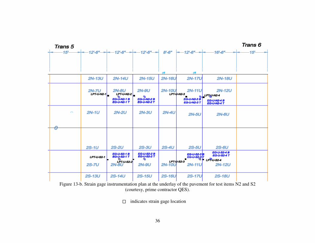
Figure 13-b. Strain gage instrumentation plan at the underlay of the pavement for test items N2 and S2
(courtesy, prime contractor QES).
indicates strain gage location
37
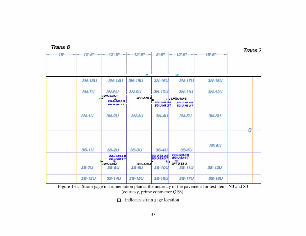
Figure 13-c. Strain gage instrumentation plan at the underlay of the pavement for test items N3 and S3
(courtesy, prime contractor QES).
indicates strain gage location

38
Figure 14-a. Strain gage instrumentation plan at the overlay of the pavement for test items N1 and S1
(courtesy, prime contractor QES).
indicates strain gage location
39
Figure 14-b. Strain Gage instrumentation plan at the overlay of the pavement for test items N2 and S2
(courtesy, prime contractor QES).
indicates strain gage location
40
Figure 14-c. Strain Gage instrumentation plan at the overlay of the pavement for test items N3 and S3
(courtesy, prime contractor QES).
indicates strain gage location
41
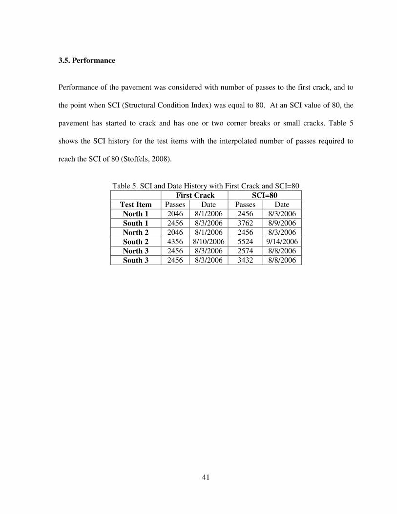
3.5. Performance
Performance of the pavement was considered with number of passes to the first crack, and to
the point when SCI (Structural Condition Index) was equal to 80. At an SCI value of 80, the
pavement has started to crack and has one or two corner breaks or small cracks. Table 5
shows the SCI history for the test items with the interpolated number of passes required to
reach the SCI of 80 (Stoffels, 2008).
Table 5. SCI and Date History with First Crack and SCI=80
First Crack SCI=80
Test Item Passes Date Passes Date
North 1 2046 8/1/2006 2456 8/3/2006
South 1 2456 8/3/2006 3762 8/9/2006
North 2 2046 8/1/2006 2456 8/3/2006
South 2 4356 8/10/2006 5524 9/14/2006
North 3 2456 8/3/2006 2574 8/8/2006
South 3 2456 8/3/2006 3432 8/8/2006
42
CHAPTER 4. METHODOLOGY
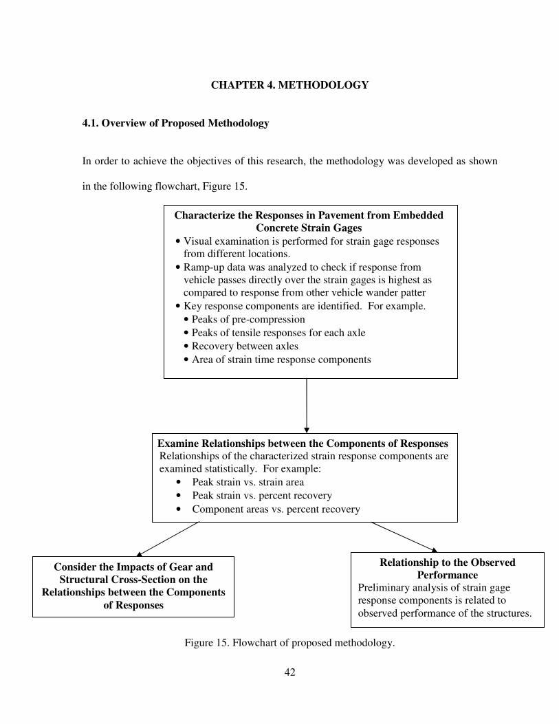
4.1. Overview of Proposed Methodology
In order to achieve the objectives of this research, the methodology was developed as shown
in the following flowchart, Figure 15.
Figure 15. Flowchart of proposed methodology.
Characterize the Responses in Pavement from Embedded
Concrete Strain Gages
• Visual examination is performed for strain gage responses
from different locations.
• Ramp-up data was analyzed to check if response from
vehicle passes directly over the strain gages is highest as
compared to response from other vehicle wander patter
• Key response components are identified. For example.
• Peaks of pre-compression
• Peaks of tensile responses for each axle
• Recovery between axles
• Area of strain time response components
Examine Relationships between the Components of Responses
Relationships of the characterized strain response components are
examined statistically. For example:
• Peak strain vs. strain area
• Peak strain vs. percent recovery
• Component areas vs. percent recovery
Consider the Impacts of Gear and
Structural Cross-Section on the
Relationships between the Components
of Responses
Relationship to the Observed
Performance
Preliminary analysis of strain gage
response components is related to
observed performance of the structures.
43
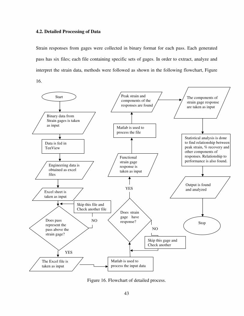
4.2. Detailed Processing of Data
Strain responses from gages were collected in binary format for each pass. Each generated
pass has six files; each file containing specific sets of gages. In order to extract, analyze and
interpret the strain data, methods were followed as shown in the following flowchart, Figure
16.
Figure 16. Flowchart of detailed process.
Statistical analysis is done
to find relationship between
peak strain, % recovery and
other components of
responses. Relationship to
performance is also found. Functional
strain gage
response is
taken as input
Peak strain and
components of the
responses are found
Matlab is used to
process the file
Output is found
and analyzed
Stop
The components of
strain gage responses
are taken as input
Start
Binary data from
Strain gages is taken
as input
Engineering data is
obtained as excel
files
Data is fed in
TenView
Does pass
represent the
pass above the
strain gage?
Matlab is used to
process the input data The Excel file is
taken as input
Does strain
gage have
response?
Excel sheet is
taken as input
Skip this file and
Check another file
NO
YES
Skip this gage and
Check another
NO
YES
44
4.2.1. Data Extraction/Filtering. Extracting strain gage data from binary files is the first
step. Before the first crack, there were a total of 4356 vehicle passes. Each pass has 6 files
containing gage responses from different locations. FAA Tenview takes nearly 7 min to
extract one binary file to an Excel spreadsheet. In order to extract the entire datasets, it would
have taken over 508 hours of continuous extraction. Since FAA Tenview was not designed to
extract more than one file at time (the code was principally written for visually monitoring
data near the time of collection), it was necessary to modify and automate Tenview to increase
the speed and to extract all the possible passes. After Tenview was modified, responses were
removed from the gages other than strain gages, and stored for later analysis efforts. Then data
from vehicle passes directly above the strain gages were selected as input for the subsequent
steps.
4.2.2. Responses from Track 0. Since, track 0 (track number for the wander position when
the outside wheel track of the gear passes directly over the strain gages) responses were used
to process and analyze datasets, it was verified that the responses from track 0 yielded higher
response values as compared to responses from other datasets.
Before the full-scale baseline experiment started on 25th
July, 2006, the cross-sections were
preloaded with triple dual tandem and twin dual tandem gears at wheel loads in incremental
increases as listed in Table 3. The responses captured by the gages were used to check if the
track, when vehicle passes directly over the strain, gives higher and better peak strain
response. Peak strain response from all the gages was calculated for all passes. Then average
was taken for one full wander which contains a total of 66 passes for each gage and every
track. Figure 17, as prepared by doctoral candidate Lin Yeh, shows the response for test item

45
1 from triple dual tandem loading. Similar plots were prepared for all test items to verify that
responses were consistently higher at track 0 for all wheel loads, cross-sections and gage
positions
Figure 17. Strain gage average responses from one wander of ramp-up loading for gages in
test item north 1 with triple dual tandem loading (courtesy, Lin Yeh).
4.2.3. Matlab Programming. Development and programming of this methodology was a
primary part of the thesis work. In addition, potential descriptive components of the total
strain gage responses were developed, including peak values, recovery between axles, and
area components of the strain response. Initially, Visual Basic was used to further analyze the
data and find peak responses. Because of its capability as engineering software, Matlab was
chosen to do all the subsequent analysis including the computation of peak responses and the
-150
-100
-50
0
50
100
150
-4 -3 -2 -1 0 1 2 3 4
Str
ain
Gage
Aver
age
Res
pon
se o
f on
e w
an
der
of
40k
(mic
roS
train
)
Track Number
EG-U-N1-1 B EG-U-N1-1 T EG-U-N1-2 B EG-U-N1-2 TEG-U-N1-3 B EG-U-N1-3 T EG-O-N1-1 B EG-O-N1-1 TEG-O-N1-2 B EG-O-N1-2 T EG-O-N1-3 B EG-O-N1-3 T
46
component areas under the strain responses. Matlab programming helped to remove the strain
gage responses which were either bad or had no data. Also, it helped to automate the data as
two responses from strain gages at two different locations were not the same in pattern.
Initially, portions of the strain response graphs were defined. The definitions used are as
follows:
Baseline: As shown in Figure 18, baseline of a strain gage response is the value shown by an
unloaded strain gage. The baseline is used as a relative x-axis to calculate peak strain and
other components of the strain gage response.
Figure 18. Baseline for a strain gage response.
Percent recovery: Figure 19 shows a typical strain gage response when it was loaded with
triple dual tandem gear. As a result of loading by three axles, three strain peaks were
generated, shown in Figure 19 as “peak 1”, “peak 2” and “peak 3”. When the loading shifted
from one of three axles to the second axle, the pavement recovered with strain gage for that
time period. The recovery was recorded by the strain gage and is shown in Figure 19 as
0
5
10
15
20
25
30
35
40
0 100 200 300 400 500 600 700 800 900
mic
roS
train
Number of Cycles
Baseline
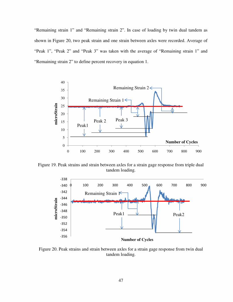
47
“Remaining strain 1” and “Remaining strain 2”. In case of loading by twin dual tandem as
shown in Figure 20, two peak strain and one strain between axles were recorded. Average of
“Peak 1”, “Peak 2” and “Peak 3” was taken with the average of “Remaining strain 1” and
“Remaining strain 2” to define percent recovery in equation 1.
Figure 19. Peak strains and strain between axles for a strain gage response from triple dual
tandem loading.
Figure 20. Peak strains and strain between axles for a strain gage response from twin dual
tandem loading.
0
5
10
15
20
25
30
35
40
0 100 200 300 400 500 600 700 800 900
mic
roS
train
Number of Cycles
Remaining Strain 1
Remaining Strain 2
Peak1Peak 2 Peak 3
-356
-354
-352
-350
-348
-346
-344
-342
-340
-338
0 100 200 300 400 500 600 700 800 900
mic
roS
train
Number of Cycles
Peak1 Peak2
Remaining Strain 1
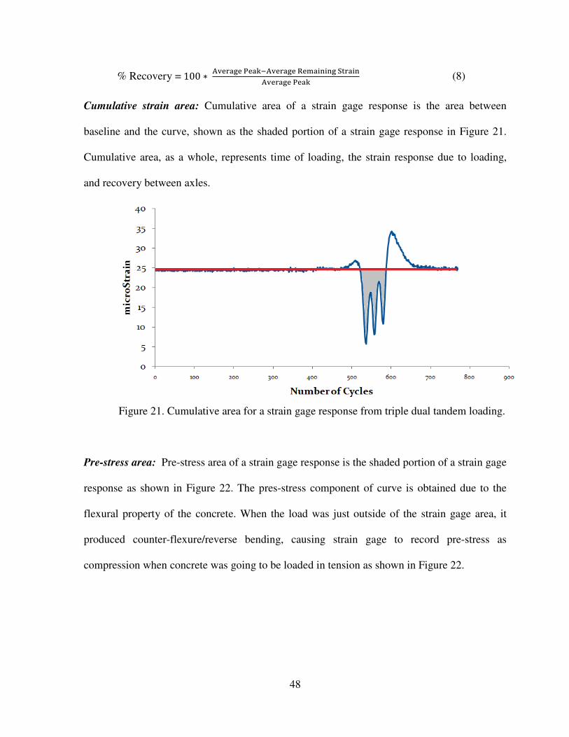
48
% Recovery = 100 ∗ 9:;<=�; >;=?�9:;<=�; *;@=ABAB� )C<=AB9:;<=�; >;=? (8)
Cumulative strain area: Cumulative area of a strain gage response is the area between
baseline and the curve, shown as the shaded portion of a strain gage response in Figure 21.
Cumulative area, as a whole, represents time of loading, the strain response due to loading,
and recovery between axles.
Figure 21. Cumulative area for a strain gage response from triple dual tandem loading.
Pre-stress area: Pre-stress area of a strain gage response is the shaded portion of a strain gage
response as shown in Figure 22. The pres-stress component of curve is obtained due to the
flexural property of the concrete. When the load was just outside of the strain gage area, it
produced counter-flexure/reverse bending, causing strain gage to record pre-stress as
compression when concrete was going to be loaded in tension as shown in Figure 22.
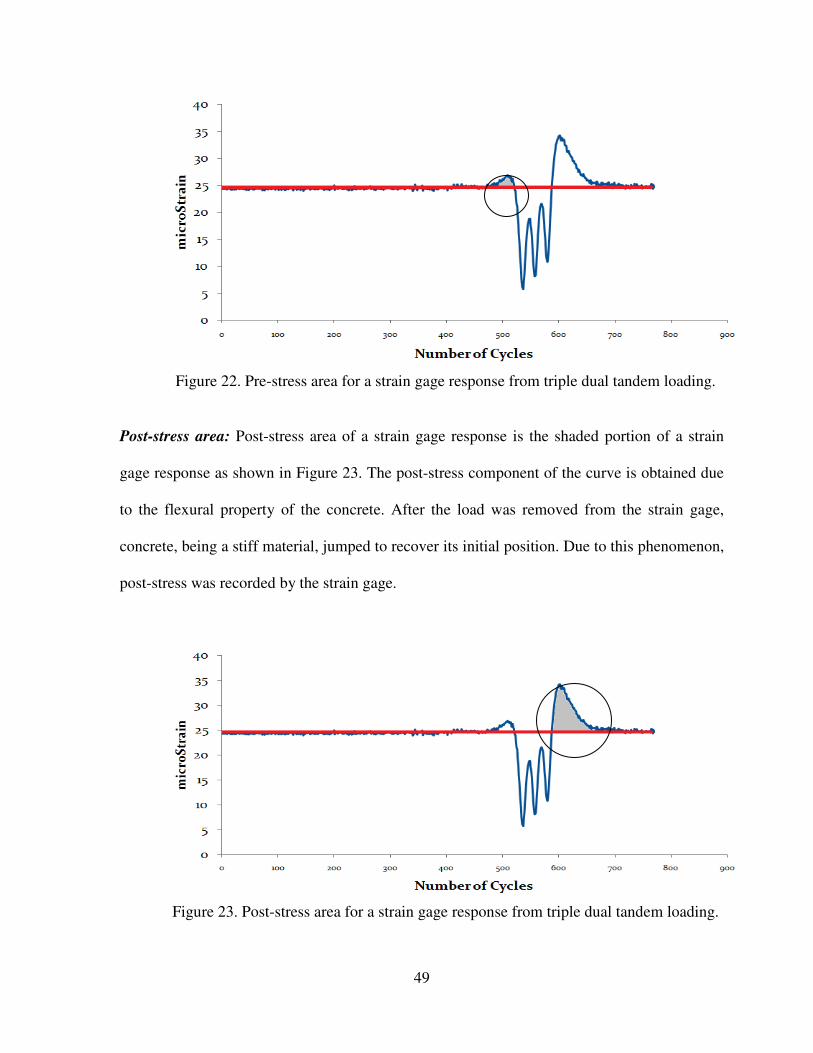
49
Figure 22. Pre-stress area for a strain gage response from triple dual tandem loading.
Post-stress area: Post-stress area of a strain gage response is the shaded portion of a strain
gage response as shown in Figure 23. The post-stress component of the curve is obtained due
to the flexural property of the concrete. After the load was removed from the strain gage,
concrete, being a stiff material, jumped to recover its initial position. Due to this phenomenon,
post-stress was recorded by the strain gage.
Figure 23. Post-stress area for a strain gage response from triple dual tandem loading.
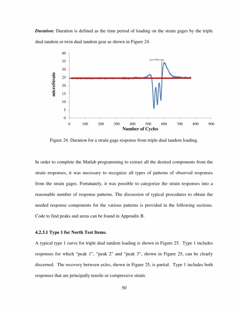
Duration: Duration is defined as the time period of loading on the strain gages by the triple
dual tandem or twin dual tandem gear as shown in Figure
Figure 24. Duration for a strain gage response from triple dual tandem loading.
In order to complete the Matlab programming
strain responses, it was necessary to recognize all types of patterns of observed responses
from the strain gages. Fortunately, it was possible to categorize the strain responses into a
reasonable number of response patterns. The discussion of typical procedures to obtain the
needed response components for the various patterns is provided in the following sections.
Code to find peaks and areas can be found in Appendix
4.2.3.1 Type 1 for North Test Item
A typical type 1 curve for triple dual tandem loading is shown in Figure 2
responses for which “peak 1”, “peak 2” and “peak 3”, shown in Figure 2
discerned. The recovery between axles
responses that are principally tensile or compressive strain.
0
5
10
15
20
25
30
35
40
0 100
mic
roS
train
50
Duration is defined as the time period of loading on the strain gages by the triple
dual tandem or twin dual tandem gear as shown in Figure 24.
. Duration for a strain gage response from triple dual tandem loading.
he Matlab programming to extract all the desired components from the
, it was necessary to recognize all types of patterns of observed responses
from the strain gages. Fortunately, it was possible to categorize the strain responses into a
easonable number of response patterns. The discussion of typical procedures to obtain the
needed response components for the various patterns is provided in the following sections.
Code to find peaks and areas can be found in Appendix B.
North Test Items.
A typical type 1 curve for triple dual tandem loading is shown in Figure 25.
“peak 1”, “peak 2” and “peak 3”, shown in Figure 2
The recovery between axles, shown in Figure 25, is partial. Type 1 includes both
responses that are principally tensile or compressive strain.
200 300 400 500 600 700
Number of Cycles
Duration is defined as the time period of loading on the strain gages by the triple
. Duration for a strain gage response from triple dual tandem loading.
to extract all the desired components from the
, it was necessary to recognize all types of patterns of observed responses
from the strain gages. Fortunately, it was possible to categorize the strain responses into a
easonable number of response patterns. The discussion of typical procedures to obtain the
needed response components for the various patterns is provided in the following sections.
. Type 1 includes
“peak 1”, “peak 2” and “peak 3”, shown in Figure 25, can be clearly
Type 1 includes both
700 800 900
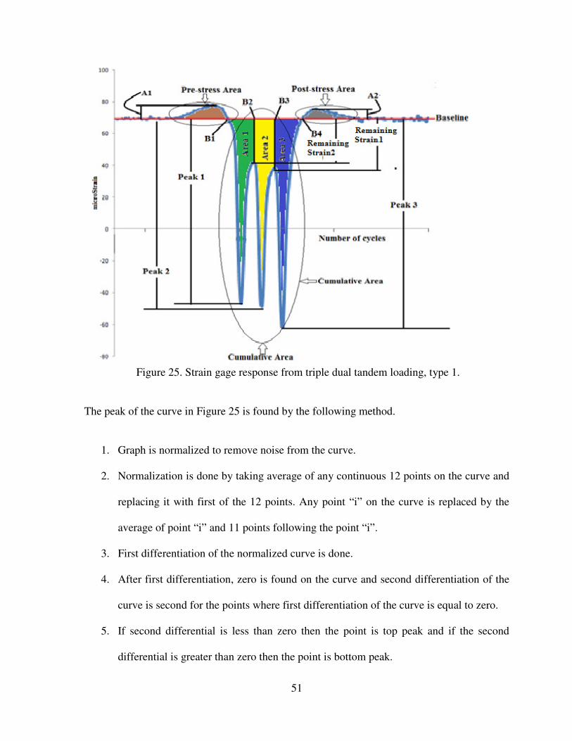
51
Figure 25. Strain gage response from triple dual tandem loading, type 1.
The peak of the curve in Figure 25 is found by the following method.
1. Graph is normalized to remove noise from the curve.
2. Normalization is done by taking average of any continuous 12 points on the curve and
replacing it with first of the 12 points. Any point “i” on the curve is replaced by the
average of point “i” and 11 points following the point “i”.
3. First differentiation of the normalized curve is done.
4. After first differentiation, zero is found on the curve and second differentiation of the
curve is second for the points where first differentiation of the curve is equal to zero.
5. If second differential is less than zero then the point is top peak and if the second
differential is greater than zero then the point is bottom peak.

52
Area under the curve for strain responses of the type shown in Figure 25 is calculated by the
following methods.
1. First “base-line” for the curve is chosen by taking the average of first 100 value or last
100 values (average for last 100 values were taken in this case to find baseline). Red
horizontal line in Figure 25 resembles the baseline for the curve.
2. Graph was normalized using Matlab to remove noise.
3. In order to find the area of the curve, “base – line” for a graph is shifted to 0.
4. The graph is then divided in two graphs, one above base line and other below base
line.
5. The graph above base-line is named as Graph A and the graph below baseline as
Graph B.
6. Peak Values for Graph B (graph below “base-line”) are found.
7. Then area under the curve B was found using peak value. The Area is divided into
three areas, Area 1 (area between baseline and curve from point B1 to B2), Area2
(area between baseline and curve from point B2 to B3) and Area3 (area between
baseline and curve from point B3 to B4).
a) Type 1 has three top peak and four bottom peaks for the curve B.
b) In order to find the area1, area2 and area3, it is important to know the B1, B2, B3
and B4.
8. Same steps are followed for Graph A, i.e., peak values were found and the area under
the curve, i.e., pre-stress area and post-stress area, show in Figure 25, was found using
the peak value.

53
a) For pre-stress and post-stress, Graph A for every type has same combination of
two top peaks, shown as A1 and A2 in Figure 25, and four bottom peaks, when
strain is equal to baseline. So, there was no change in argument for this for any
types of the curve.
To find area values B1, B2, B3 and B4 are calculated. These values are used to calculate
recovery between axles.
4.2.3.2 Type 2 for North Test Items.
Type 2 curves are similar to type 1, except that full recovery of tensile or compressive strains
may occur between some axles, shown in Figure 26 as remaining strains touching the
baseline.
Figure 26. Strain gage response from triple dual tandem loading, type 2.
Area under the above curve for this type is calculated by following methods.

54
1. First “base-line” for the curve is chosen by taking the average of first 100 value or last
100 values (average for last 100 values were taken in this case to find baseline).
2. Graph was normalized using Matlab to remove noise.
3. In order to find the area of the curve, “base – line” for a graph is shifted to 0.
4. The graph is then divided in two graphs, one above base line and other below base
line.
5. The graph above base-line is named as Graph A and the graph below baseline as
Graph B.
6. Peak Values for Graph B (graph below “base-line”) are found.
7. Then area under the curve B was found using peak value. The Area is divided into
three areas, Area 1 (area between baseline and curve from point B1 to B2), Area2
(area between baseline and curve from point B2 to B3) and Area3 (area between
baseline and curve from point B3 to B4).
a) Type 2 has three top peak and four bottom peaks for the curve B similar to TYPE1.
b) In order to find the area1, area2 and area3, it is important to know the B1, B2, B3
and B4.
8. Same steps are followed for Graph A, i.e., peak values were found and the area under
the curve, i.e., pre-stress area and post-stress area, as shown in Figure 26, were found
using the peak value.
a) For pre-load and post-load, Graph A for every type has same combination of two top
peaks, A1 and A2 in Figure 26, and four bottom peaks, when strain is equal to
baseline. So, there was no change in argument for this for any types of the curve.
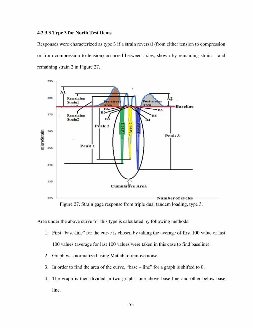
55
4.2.3.3 Type 3 for North Test Items
Responses were characterized as type 3 if a strain reversal (from either tension to compression
or from compression to tension) occurred between axles, shown by remaining strain 1 and
remaining strain 2 in Figure 27.
Figure 27. Strain gage response from triple dual tandem loading, type 3.
Area under the above curve for this type is calculated by following methods.
1. First “base-line” for the curve is chosen by taking the average of first 100 value or last
100 values (average for last 100 values were taken in this case to find baseline).
2. Graph was normalized using Matlab to remove noise.
3. In order to find the area of the curve, “base – line” for a graph is shifted to 0.
4. The graph is then divided in two graphs, one above base line and other below base
line.

56
5. The graph above base-line is named as Graph A and the graph below baseline as
Graph B.
6. Peak Values for Graph B (graph below “base-line”) are found.
7. Then area under the curve B was found using peak value. The Area is divided into
three areas, Area 1 (area between baseline and curve from point B1 to B2), Area2
(area between baseline and curve from point B3 to B4) and Area3 (area between
baseline and curve from point B5 to B6).
a) Type 3 has three top peak and six bottom peaks for the curve B
b) In order to find the area1, area2 and area3, it is important to know the B1, B2, B3,
B4, B5 and B6.
8. Same steps are followed for Graph A, i.e., peak values were found and the area under
the curve, i.e., pre-stress area and post-stress area, as shown in Figure 27, were found
using the peak value.
b) For pre-stress and post-stress, Graph A for every type has same combination of two
top peaks, A1 and A2 in Figure 27, and four bottom peaks, when strain is equal to
baseline. So, there was no change in argument for this for any types of the curve.
4.2.3.4 Type 4 for North Test Items.
Responses were characterized as type 4 if a strain reversal (from either tension to
compression, or from compression to tension), shown by remaining strain2 in Figure 28,
occurred between only a single set of axles.
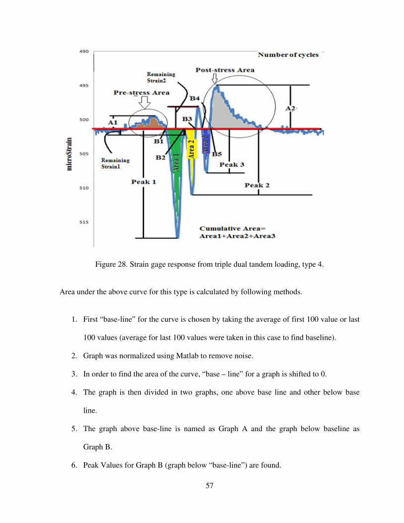
57
Figure 28. Strain gage response from triple dual tandem loading, type 4.
Area under the above curve for this type is calculated by following methods.
1. First “base-line” for the curve is chosen by taking the average of first 100 value or last
100 values (average for last 100 values were taken in this case to find baseline).
2. Graph was normalized using Matlab to remove noise.
3. In order to find the area of the curve, “base – line” for a graph is shifted to 0.
4. The graph is then divided in two graphs, one above base line and other below base
line.
5. The graph above base-line is named as Graph A and the graph below baseline as
Graph B.
6. Peak Values for Graph B (graph below “base-line”) are found.

58
7. Then area under the curve B was found using peak value. The Area is divided into
three areas, Area 1 (area between baseline and curve from point B1 to B2), Area2
(area between baseline and curve from point B3 to B4) and Area3 (area between
baseline and curve from point B4 to B5).
a) Type 4 has three top peak and five bottom peaks for the curve B
b) In order to find the area1, area2 and area3, it is important to know the B1, B2, B3,
B4, B5 and B6.
9. Same steps are followed for Graph A, i.e., peak values were found and the area under
the curve, i.e., pre-stress area and post-stress area, as shown in Figure 28, were found
using the peak value.
c) For pre-stress and post-stress, Graph A for every type has same combination of two
top peaks, A1 and A2 in Figure 28, and four bottom peaks, when strain is equal to
baseline. So, there was no change in argument for this for any types of the curve.
4.2.3.5 Types 1, 2 and 3 for South Test Items.
Loading on the south test items was conducted with a twin dual tandem gear with two axles.
As a result, responses captured by the strain gages have 5 peaks which are categorized in
following types from 1 to 4. Finding areas for these types is similar to finding areas for the
response patterns observed in the north test items.
The following types of strain response patterns can be related to the typical response pattern
types for the north test items.
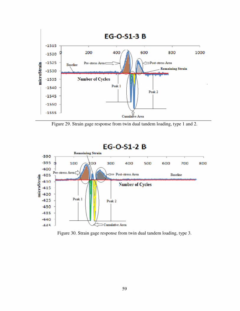
59
Figure 29. Strain gage response from twin dual tandem loading, type 1 and 2.
Figure 30. Strain gage response from twin dual tandem loading, type 3.
60
4.2.4. Statistical Analysis
After extracting and filtering data, statistical analysis on the data was done to extract
information from the data sets. There were a total of 64 strain gages installed for the Baseline
Experiment. It was important to analyze and characterize all the strain gages and to check the
behavior of the peak values, recovery between axles, and area components of the strain
response for each of the strain gages. Statistical analysis was done in Excel with the help of
Excel’s Visual Basic for Applications (VBA).
After characterizing the components of strain gage responses in terms of both mean and
standard deviation, each of the components was correlated to check its dependency on other
components. Then regression analysis was done on key components which are independent to
each other. To do the correlation and regression analysis, the whole dataset was divided by
pavement cross-section and loading configuration.
Strain gage response components were analyzed with number of passes to reach an SCI value
of 80 for the preliminary examination of the performance of the pavement at different cross-
sections with the two loading conditions. The numbers of passes to an SCI value of 80 were
chosen above number of passes to first crack because the first crack was not always seen
immediately during the course of loading on the test items. Practically, it was therefore not
possible to obtain the exact number of passes to the first crack. However, the number of
passes to “SCI=80” could be interpolated from SCI values at the end of loading for each day.
The effect of number of axles was included in all attempts to develop regression models for
the test items. This was necessary for a number of reasons, including that the total applied

61
gear load was directly proportional to the number of axles. For all regression models and
correlations, Excel 2007 was used with Visual Basic for Applications (VBA).
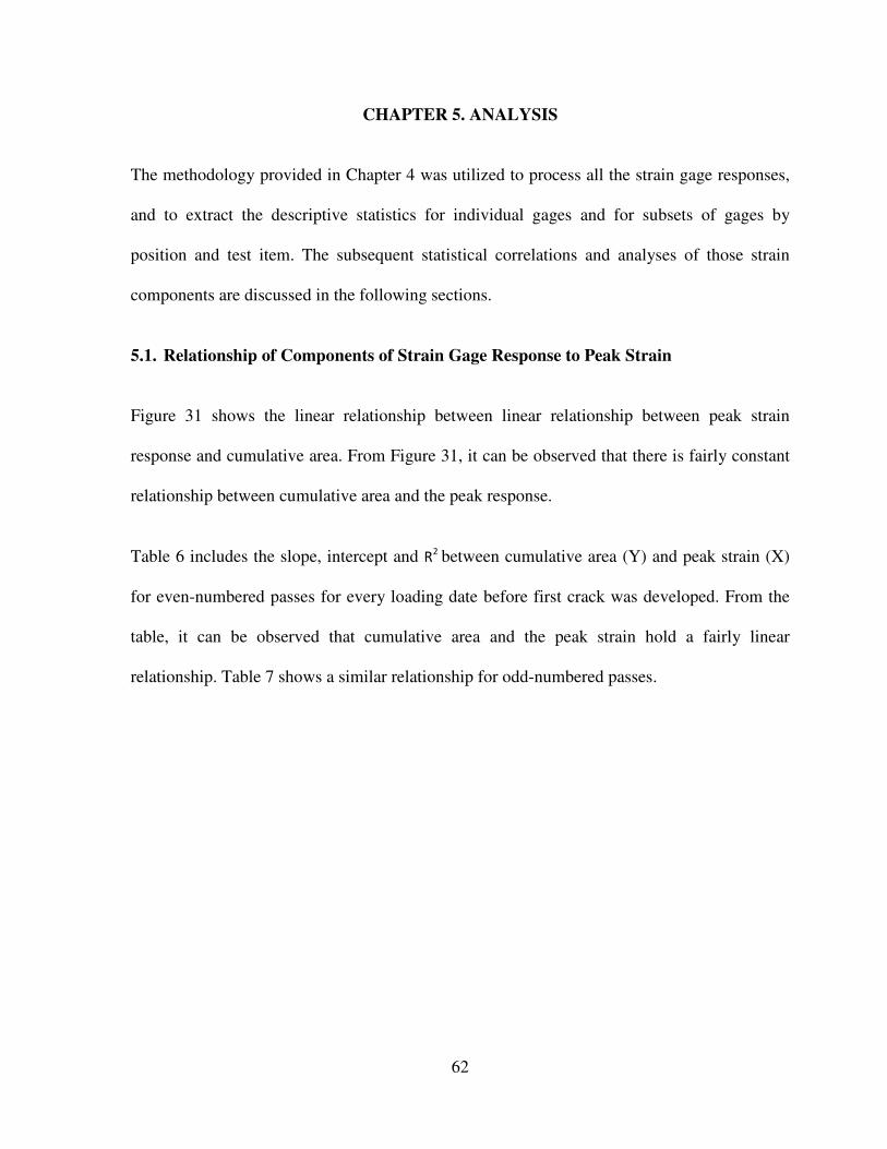
62
CHAPTER 5. ANALYSIS
The methodology provided in Chapter 4 was utilized to process all the strain gage responses,
and to extract the descriptive statistics for individual gages and for subsets of gages by
position and test item. The subsequent statistical correlations and analyses of those strain
components are discussed in the following sections.
5.1. Relationship of Components of Strain Gage Response to Peak Strain
Figure 31 shows the linear relationship between linear relationship between peak strain
response and cumulative area. From Figure 31, it can be observed that there is fairly constant
relationship between cumulative area and the peak response.
Table 6 includes the slope, intercept and R2 between cumulative area (Y) and peak strain (X)
for even-numbered passes for every loading date before first crack was developed. From the
table, it can be observed that cumulative area and the peak strain hold a fairly linear
relationship. Table 7 shows a similar relationship for odd-numbered passes.
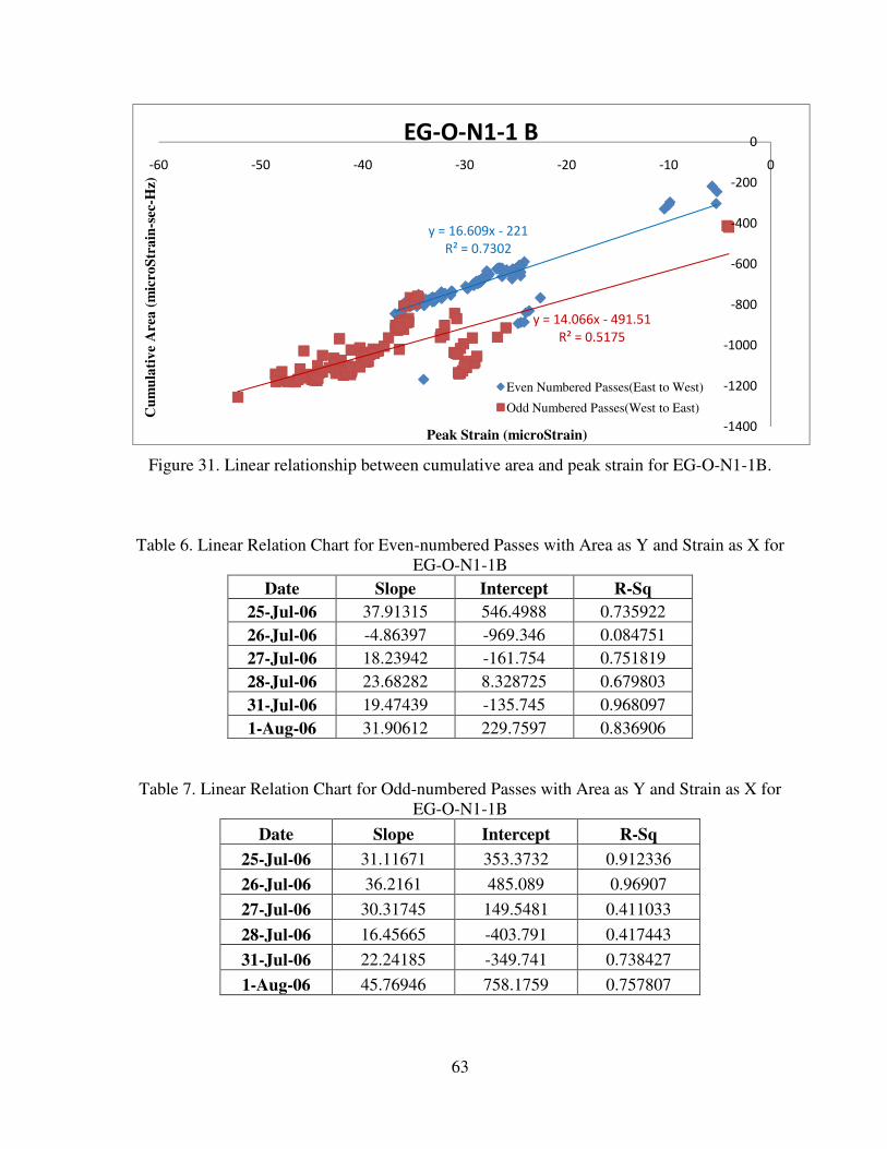
63
Figure 31. Linear relationship between cumulative area and peak strain for EG-O-N1-1B.
Table 6. Linear Relation Chart for Even-numbered Passes with Area as Y and Strain as X for
EG-O-N1-1B
Date Slope Intercept R-Sq
25-Jul-06 37.91315 546.4988 0.735922
26-Jul-06 -4.86397 -969.346 0.084751
27-Jul-06 18.23942 -161.754 0.751819
28-Jul-06 23.68282 8.328725 0.679803
31-Jul-06 19.47439 -135.745 0.968097
1-Aug-06 31.90612 229.7597 0.836906
Table 7. Linear Relation Chart for Odd-numbered Passes with Area as Y and Strain as X for
EG-O-N1-1B
Date Slope Intercept R-Sq
25-Jul-06 31.11671 353.3732 0.912336
26-Jul-06 36.2161 485.089 0.96907
27-Jul-06 30.31745 149.5481 0.411033
28-Jul-06 16.45665 -403.791 0.417443
31-Jul-06 22.24185 -349.741 0.738427
1-Aug-06 45.76946 758.1759 0.757807
y = 16.609x - 221
R² = 0.7302
y = 14.066x - 491.51
R² = 0.5175
-1400
-1200
-1000
-800
-600
-400
-200
0
-60 -50 -40 -30 -20 -10 0C
um
ula
tiv
e A
rea
(m
icro
Str
ain
-sec
-Hz)
Peak Strain (microStrain)
EG-O-N1-1 B
Even Numbered Passes(East to West)
Odd Numbered Passes(West to East)
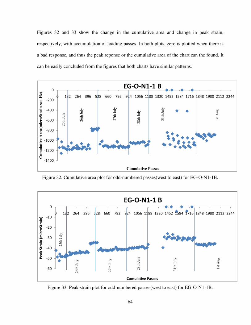
64
Figures 32 and 33 show the change in the cumulative area and change in peak strain,
respectively, with accumulation of loading passes. In both plots, zero is plotted when there is
a bad response, and thus the peak reponse or the cumulative area of the chart can the found. It
can be easily concluded from the figures that both charts have similar patterns.
Figure 32. Cumulative area plot for odd-numbered passes(west to east) for EG-O-N1-1B.
Figure 33. Peak strain plot for odd-numbered passes(west to east) for EG-O-N1-1B.
-1400
-1200
-1000
-800
-600
-400
-200
0
0 132 264 396 528 660 792 924 1056 1188 1320 1452 1584 1716 1848 1980 2112 2244
Cu
mu
lati
ve
Are
a(m
icro
Str
ain
-sec
-Hz)
Cumulative Passes
EG-O-N1-1 B
25
th J
uly
26
th J
uly
27
th J
uly
28
th J
uly
31
th J
uly
1st
Au
g
-60
-50
-40
-30
-20
-10
0
0 132 264 396 528 660 792 924 1056 1188 1320 1452 1584 1716 1848 1980 2112 2244
Pe
ak
Str
ain
(m
icro
Str
ain
)
Cumulative Passes
EG-O-N1-1 B
25
th J
uly
26
th J
uly
27
th J
uly
28
th J
uly
31
th J
uly
1st
Au
g
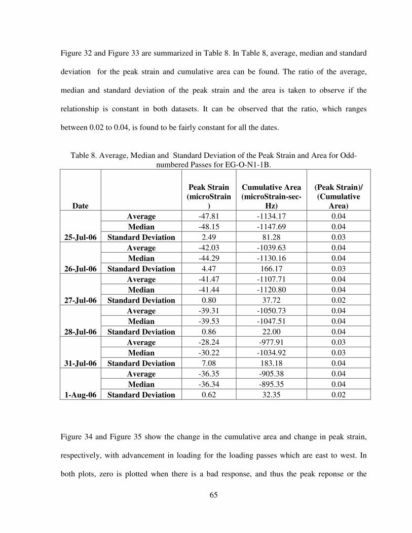
65
Figure 32 and Figure 33 are summarized in Table 8. In Table 8, average, median and standard
deviation for the peak strain and cumulative area can be found. The ratio of the average,
median and standard deviation of the peak strain and the area is taken to observe if the
relationship is constant in both datasets. It can be observed that the ratio, which ranges
between 0.02 to 0.04, is found to be fairly constant for all the dates.
Table 8. Average, Median and Standard Deviation of the Peak Strain and Area for Odd-
numbered Passes for EG-O-N1-1B.
Date
Peak Strain
(microStrain
)
Cumulative Area
(microStrain-sec-
Hz)
(Peak Strain)/
(Cumulative
Area)
25-Jul-06
Average -47.81 -1134.17 0.04
Median -48.15 -1147.69 0.04
Standard Deviation 2.49 81.28 0.03
26-Jul-06
Average -42.03 -1039.63 0.04
Median -44.29 -1130.16 0.04
Standard Deviation 4.47 166.17 0.03
27-Jul-06
Average -41.47 -1107.71 0.04
Median -41.44 -1120.80 0.04
Standard Deviation 0.80 37.72 0.02
28-Jul-06
Average -39.31 -1050.73 0.04
Median -39.53 -1047.51 0.04
Standard Deviation 0.86 22.00 0.04
31-Jul-06
Average -28.24 -977.91 0.03
Median -30.22 -1034.92 0.03
Standard Deviation 7.08 183.18 0.04
1-Aug-06
Average -36.35 -905.38 0.04
Median -36.34 -895.35 0.04
Standard Deviation 0.62 32.35 0.02
Figure 34 and Figure 35 show the change in the cumulative area and change in peak strain,
respectively, with advancement in loading for the loading passes which are east to west. In
both plots, zero is plotted when there is a bad response, and thus the peak reponse or the
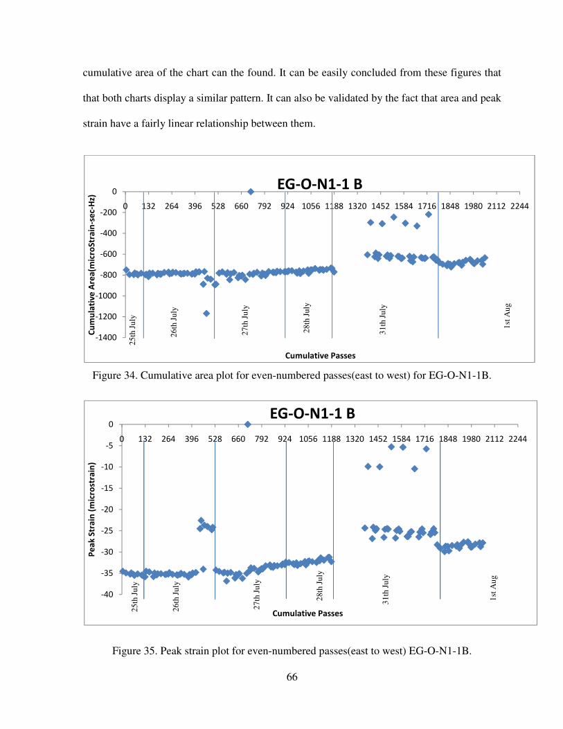
66
cumulative area of the chart can the found. It can be easily concluded from these figures that
that both charts display a similar pattern. It can also be validated by the fact that area and peak
strain have a fairly linear relationship between them.
Figure 34. Cumulative area plot for even-numbered passes(east to west) for EG-O-N1-1B.
Figure 35. Peak strain plot for even-numbered passes(east to west) EG-O-N1-1B.
-1400
-1200
-1000
-800
-600
-400
-200
0
0 132 264 396 528 660 792 924 1056 1188 1320 1452 1584 1716 1848 1980 2112 2244
Cu
mu
lati
ve
Are
a(m
icro
Str
ain
-se
c-H
z)
Cumulative Passes
EG-O-N1-1 B
25
th J
uly
26
th J
uly
27
th J
uly
28
th J
uly
31
th J
uly
1st
Au
g
-40
-35
-30
-25
-20
-15
-10
-5
0
0 132 264 396 528 660 792 924 1056 1188 1320 1452 1584 1716 1848 1980 2112 2244
Pe
ak
Str
ain
(m
icro
stra
in)
Cumulative Passes
EG-O-N1-1 B
26
th J
uly
27
th J
uly
1st
Au
g
25
th J
uly
28
th J
uly
31
th J
uly
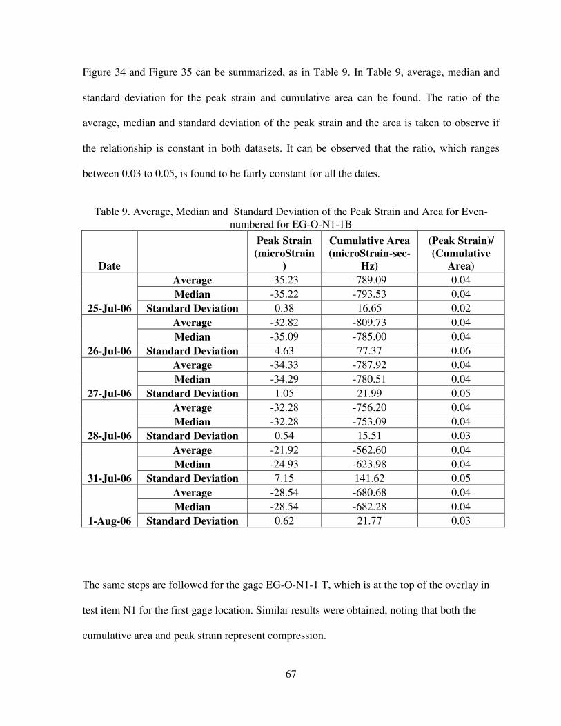
67
Figure 34 and Figure 35 can be summarized, as in Table 9. In Table 9, average, median and
standard deviation for the peak strain and cumulative area can be found. The ratio of the
average, median and standard deviation of the peak strain and the area is taken to observe if
the relationship is constant in both datasets. It can be observed that the ratio, which ranges
between 0.03 to 0.05, is found to be fairly constant for all the dates.
Table 9. Average, Median and Standard Deviation of the Peak Strain and Area for Even-
numbered for EG-O-N1-1B
Date
Peak Strain
(microStrain
)
Cumulative Area
(microStrain-sec-
Hz)
(Peak Strain)/
(Cumulative
Area)
25-Jul-06
Average -35.23 -789.09 0.04
Median -35.22 -793.53 0.04
Standard Deviation 0.38 16.65 0.02
26-Jul-06
Average -32.82 -809.73 0.04
Median -35.09 -785.00 0.04
Standard Deviation 4.63 77.37 0.06
27-Jul-06
Average -34.33 -787.92 0.04
Median -34.29 -780.51 0.04
Standard Deviation 1.05 21.99 0.05
28-Jul-06
Average -32.28 -756.20 0.04
Median -32.28 -753.09 0.04
Standard Deviation 0.54 15.51 0.03
31-Jul-06
Average -21.92 -562.60 0.04
Median -24.93 -623.98 0.04
Standard Deviation 7.15 141.62 0.05
1-Aug-06
Average -28.54 -680.68 0.04
Median -28.54 -682.28 0.04
Standard Deviation 0.62 21.77 0.03
The same steps are followed for the gage EG-O-N1-1 T, which is at the top of the overlay in
test item N1 for the first gage location. Similar results were obtained, noting that both the
cumulative area and peak strain represent compression.
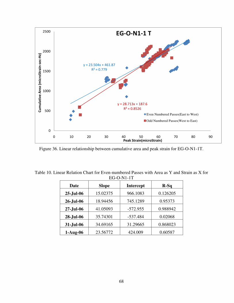
68
Figure 36. Linear relationship between cumulative area and peak strain for EG-O-N1-1T.
Table 10. Linear Relation Chart for Even-numbered Passes with Area as Y and Strain as X for
EG-O-N1-1T
Date Slope Intercept R-Sq
25-Jul-06 15.02375 966.1083 0.126205
26-Jul-06 18.94456 745.1289 0.95373
27-Jul-06 41.05093 -572.955 0.988942
28-Jul-06 35.74301 -537.484 0.02068
31-Jul-06 34.69165 31.29665 0.868023
1-Aug-06 23.56772 424.009 0.60587
y = 23.504x + 461.87
R² = 0.779
y = 28.713x + 187.6
R² = 0.8526
0
500
1000
1500
2000
2500
0 10 20 30 40 50 60 70 80 90
Cu
mu
lati
ve
Are
a (
mic
roS
tra
in-s
ec-
Hz)
Peak Strain(microStrain)
Even Numbered Passes(East to West)
Odd Numbered Passes(West to East)
EG-O-N1-1 T

69
Table 11. Linear Relation Chart for Odd-numbered Passes with Area as Y and Strain as X for
EG-O-N1-1T
Date Slope Intercept R-Sq
25-Jul-06 15.59121 836.0566 0.721136
26-Jul-06 49.95582 -1003.17 0.950624
27-Jul-06 44.60814 -726.611 0.95393
28-Jul-06 -3.36224 2146.333 0.023538
31-Jul-06 39.09608 -124.715 0.94174
1-Aug-06 46.99594 -1050.08 0.811839
Figure 37. Cumulative area plot for odd-numbered passes (west to east) for EG-O-N1-1T.
0
500
1000
1500
2000
2500
0 132 264 396 528 660 792 924 1056 1188 1320 1452 1584 1716 1848 1980 2112 2244
Cu
mu
lati
ve
Are
a (
mic
roS
tra
in-s
ec-
Hz)
Cumulative Passes
EG-O-N1-1 T
25
th J
uly
26
th J
uly
27
th J
uly
28
th J
uly
31
th J
uly
1st
Au
g
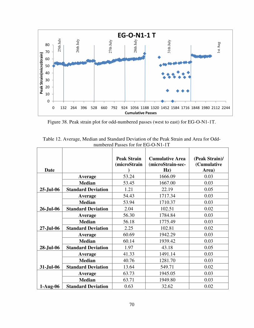
70
Figure 38. Peak strain plot for odd-numbered passes (west to east) for EG-O-N1-1T.
Table 12. Average, Median and Standard Deviation of the Peak Strain and Area for Odd-
numbered Passes for for EG-O-N1-1T
Date
Peak Strain
(microStrain
)
Cumulative Area
(microStrain-sec-
Hz)
(Peak Strain)/
(Cumulative
Area)
25-Jul-06
Average 53.24 1666.09 0.03
Median 53.45 1667.00 0.03
Standard Deviation 1.21 22.19 0.05
26-Jul-06
Average 54.43 1717.34 0.03
Median 53.94 1710.37 0.03
Standard Deviation 2.04 102.51 0.02
27-Jul-06
Average 56.30 1784.84 0.03
Median 56.18 1775.49 0.03
Standard Deviation 2.25 102.81 0.02
28-Jul-06
Average 60.69 1942.29 0.03
Median 60.14 1939.42 0.03
Standard Deviation 1.97 43.18 0.05
31-Jul-06
Average 41.33 1491.14 0.03
Median 40.76 1281.70 0.03
Standard Deviation 13.64 549.71 0.02
1-Aug-06
Average 63.73 1945.05 0.03
Median 63.71 1949.80 0.03
Standard Deviation 0.63 32.62 0.02
0
10
20
30
40
50
60
70
80
0 132 264 396 528 660 792 924 1056 1188 1320 1452 1584 1716 1848 1980 2112 2244
Pe
ak
Str
ain
(mic
roS
tra
in)
Cumulative Passes
EG-O-N1-1 T
25
th J
uly
26
th J
uly
27
th J
uly
28
th J
uly
31
th J
uly
1st
Au
g

71
Figure 39. Cumulative area plot for even-numbered passes (east to west) for EG-O-N1-1T.
Figure 40. Peak strain plot for even-numbered passes (east to west) for EG-O-N1-1T.
0
500
1000
1500
2000
2500
0 132 264 396 528 660 792 924 1056 1188 1320 1452 1584 1716 1848 1980 2112 2244
Cu
mu
lati
ve
Are
a(m
icro
Str
ain
-sec
-Hz)
Cumulative Passes
EG-O-N1-1 T
25
th J
uly
26
th J
uly
27
th J
uly
28
th J
uly
31
th J
uly
1st
Au
g
0
10
20
30
40
50
60
70
80
90
0 132 264 396 528 660 792 924 1056 1188 1320 1452 1584 1716 1848 1980 2112 2244
Pe
ak
Str
ain
(mic
roS
tra
in)
Cumulative Passes
EG-O-N1-1 T
25
th J
uly
26
th J
uly
27
th J
uly
28
th J
uly
31
th J
uly
1st
Au
g
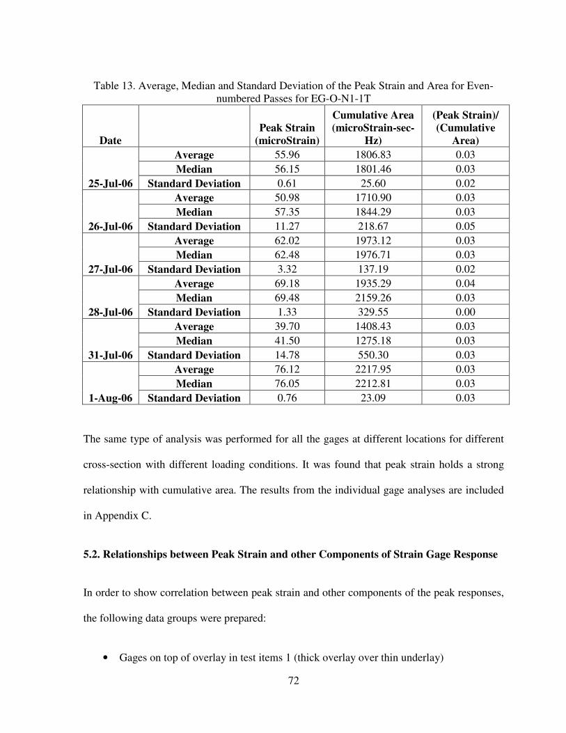
72
Table 13. Average, Median and Standard Deviation of the Peak Strain and Area for Even-
numbered Passes for EG-O-N1-1T
Date
Peak Strain
(microStrain)
Cumulative Area
(microStrain-sec-
Hz)
(Peak Strain)/
(Cumulative
Area)
25-Jul-06
Average 55.96 1806.83 0.03
Median 56.15 1801.46 0.03
Standard Deviation 0.61 25.60 0.02
26-Jul-06
Average 50.98 1710.90 0.03
Median 57.35 1844.29 0.03
Standard Deviation 11.27 218.67 0.05
27-Jul-06
Average 62.02 1973.12 0.03
Median 62.48 1976.71 0.03
Standard Deviation 3.32 137.19 0.02
28-Jul-06
Average 69.18 1935.29 0.04
Median 69.48 2159.26 0.03
Standard Deviation 1.33 329.55 0.00
31-Jul-06
Average 39.70 1408.43 0.03
Median 41.50 1275.18 0.03
Standard Deviation 14.78 550.30 0.03
1-Aug-06
Average 76.12 2217.95 0.03
Median 76.05 2212.81 0.03
Standard Deviation 0.76 23.09 0.03
The same type of analysis was performed for all the gages at different locations for different
cross-section with different loading conditions. It was found that peak strain holds a strong
relationship with cumulative area. The results from the individual gage analyses are included
in Appendix C.
5.2. Relationships between Peak Strain and other Components of Strain Gage Response
In order to show correlation between peak strain and other components of the peak responses,
the following data groups were prepared:
• Gages on top of overlay in test items 1 (thick overlay over thin underlay)
73
• Gages on top of overlay in test items 2 (equal thickness overlay and underlay)
• Gages on top of overlay in test items 3 (thin overlay over thick underlay)
• Gages on top of overlay in north test items (triple dual tandem)
• Gages on top of overlay in south test items (twin dual tandem)
• Gages on bottom of overlay in test items 1 (thick overlay over thin underlay)
• Gages on bottom of overlay in test items 2 (equal thickness overlay and underlay)
• Gages on bottom of overlay in test items 3 (thin overlay over thick underlay)
• Gages on bottom of overlay in north test items (triple dual tandem)
• Gages on bottom of overlay in south test items (twin dual tandem)
• Gages on top of underlay in test items 1 (thick overlay over thin underlay)
• Gages on top of underlay in test items 2 (equal thickness overlay and underlay)
• Gages on top of underlay in test items 3 (thin overlay over thick underlay)
• Gages on top of underlay in north test items (triple dual tandem)
• Gages on top of underlay in south test items (twin dual tandem)
• Gages on bottom of underlay in test items 1 (thin overlay over thin underlay)
• Gages on bottom of underlay in test items 2 (equal thickness overlay and underlay)
• Gages on bottom of underlay in test items 3 (thin overlay over thick underlay)
• Gages on bottom of underlay in north test items (triple dual tandem)
• Gages on bottom of underlay in south test items (twin dual tandem)
• Gages by their particular location, as shown in Figure 41 by pavement cross-section
• Gages by their particular location, as shown in Figure 41 by loading condition
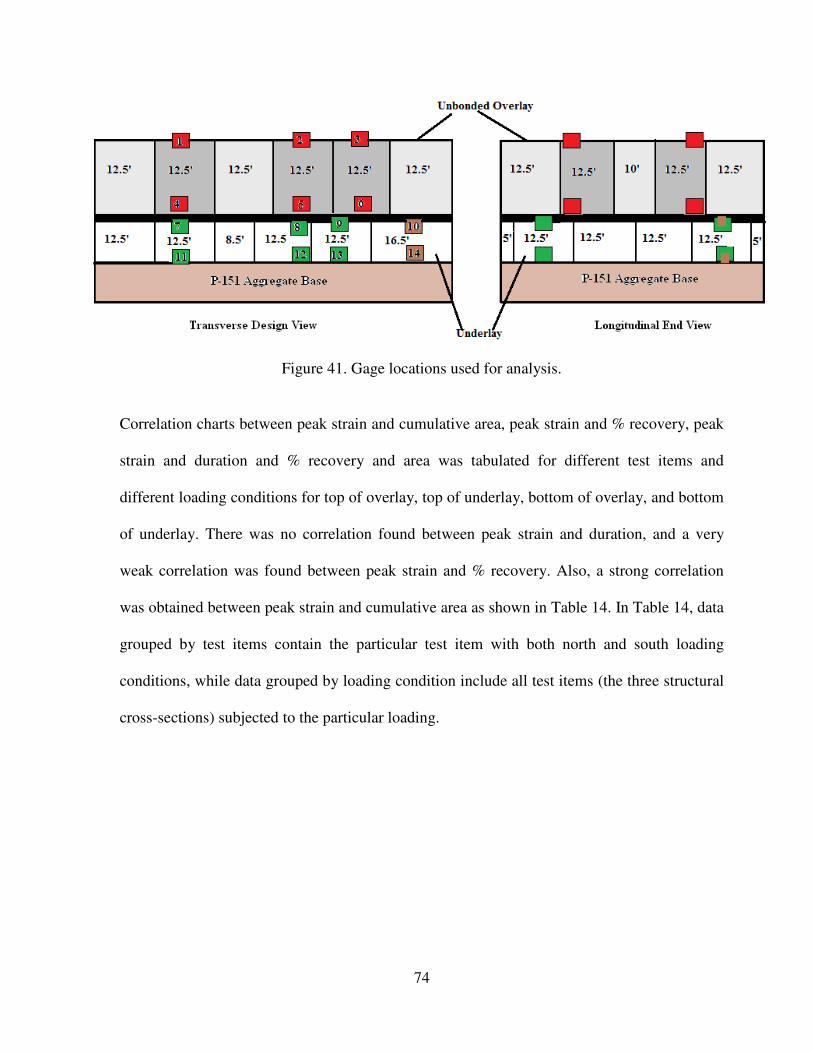
74
Figure 41. Gage locations used for analysis.
Correlation charts between peak strain and cumulative area, peak strain and % recovery, peak
strain and duration and % recovery and area was tabulated for different test items and
different loading conditions for top of overlay, top of underlay, bottom of overlay, and bottom
of underlay. There was no correlation found between peak strain and duration, and a very
weak correlation was found between peak strain and % recovery. Also, a strong correlation
was obtained between peak strain and cumulative area as shown in Table 14. In Table 14, data
grouped by test items contain the particular test item with both north and south loading
conditions, while data grouped by loading condition include all test items (the three structural
cross-sections) subjected to the particular loading.
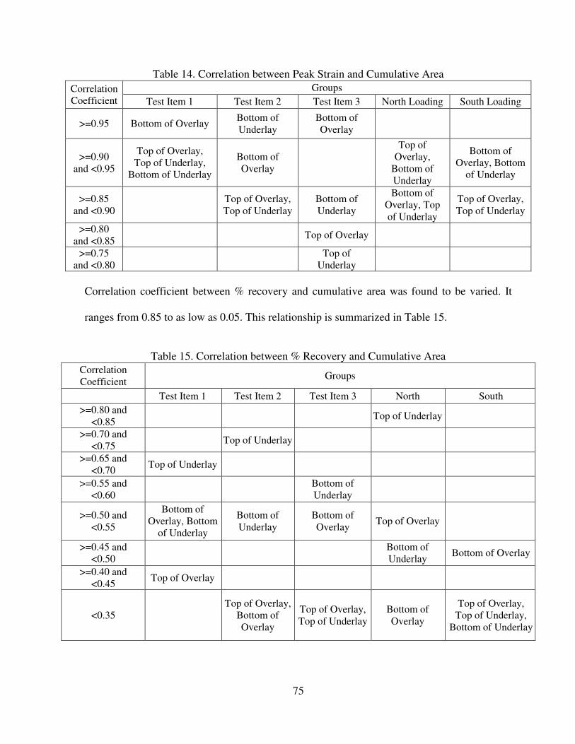
75
Table 14. Correlation between Peak Strain and Cumulative Area
Correlation
Coefficient
Groups
Test Item 1 Test Item 2 Test Item 3 North Loading South Loading
>=0.95 Bottom of Overlay Bottom of
Underlay Bottom of
Overlay
>=0.90
and <0.95
Top of Overlay,
Top of Underlay,
Bottom of Underlay
Bottom of
Overlay
Top of
Overlay,
Bottom of
Underlay
Bottom of
Overlay, Bottom
of Underlay
>=0.85
and <0.90
Top of Overlay,
Top of Underlay Bottom of
Underlay
Bottom of
Overlay, Top
of Underlay
Top of Overlay,
Top of Underlay
>=0.80
and <0.85 Top of Overlay
>=0.75
and <0.80
Top of
Underlay
Correlation coefficient between % recovery and cumulative area was found to be varied. It
ranges from 0.85 to as low as 0.05. This relationship is summarized in Table 15.
Table 15. Correlation between % Recovery and Cumulative Area
Correlation
Coefficient Groups
Test Item 1 Test Item 2 Test Item 3 North South
>=0.80 and
<0.85 Top of Underlay
>=0.70 and
<0.75 Top of Underlay
>=0.65 and
<0.70 Top of Underlay
>=0.55 and
<0.60
Bottom of
Underlay
>=0.50 and
<0.55
Bottom of
Overlay, Bottom
of Underlay
Bottom of
Underlay Bottom of
Overlay Top of Overlay
>=0.45 and
<0.50
Bottom of
Underlay Bottom of Overlay
>=0.40 and
<0.45 Top of Overlay
<0.35 Top of Overlay,
Bottom of
Overlay
Top of Overlay,
Top of Underlay Bottom of
Overlay
Top of Overlay,
Top of Underlay,
Bottom of Underlay
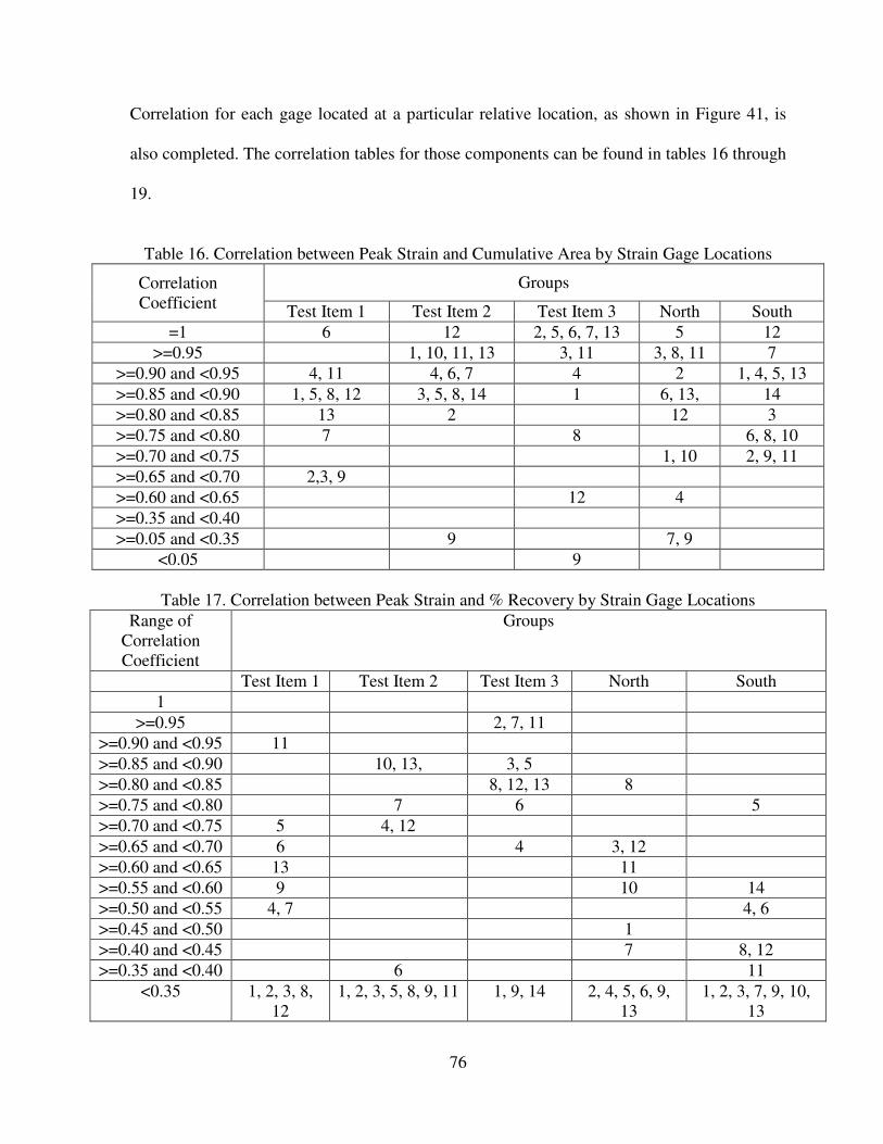
76
Correlation for each gage located at a particular relative location, as shown in Figure 41, is
also completed. The correlation tables for those components can be found in tables 16 through
19.
Table 16. Correlation between Peak Strain and Cumulative Area by Strain Gage Locations
Correlation
Coefficient
Groups
Test Item 1 Test Item 2 Test Item 3 North South
=1 6 12 2, 5, 6, 7, 13 5 12
>=0.95 1, 10, 11, 13 3, 11 3, 8, 11 7
>=0.90 and <0.95 4, 11 4, 6, 7 4 2 1, 4, 5, 13
>=0.85 and <0.90 1, 5, 8, 12 3, 5, 8, 14 1 6, 13, 14
>=0.80 and <0.85 13 2 12 3
>=0.75 and <0.80 7 8 6, 8, 10
>=0.70 and <0.75 1, 10 2, 9, 11
>=0.65 and <0.70 2,3, 9
>=0.60 and <0.65 12 4
>=0.35 and <0.40
>=0.05 and <0.35 9 7, 9
<0.05 9
Table 17. Correlation between Peak Strain and % Recovery by Strain Gage Locations
Range of
Correlation
Coefficient
Groups
Test Item 1 Test Item 2 Test Item 3 North South
1
>=0.95 2, 7, 11
>=0.90 and <0.95 11
>=0.85 and <0.90 10, 13, 3, 5
>=0.80 and <0.85 8, 12, 13 8
>=0.75 and <0.80 7 6 5
>=0.70 and <0.75 5 4, 12
>=0.65 and <0.70 6 4 3, 12
>=0.60 and <0.65 13 11
>=0.55 and <0.60 9 10 14
>=0.50 and <0.55 4, 7 4, 6
>=0.45 and <0.50 1
>=0.40 and <0.45 7 8, 12
>=0.35 and <0.40 6 11
<0.35 1, 2, 3, 8,
12
1, 2, 3, 5, 8, 9, 11 1, 9, 14 2, 4, 5, 6, 9,
13
1, 2, 3, 7, 9, 10,
13
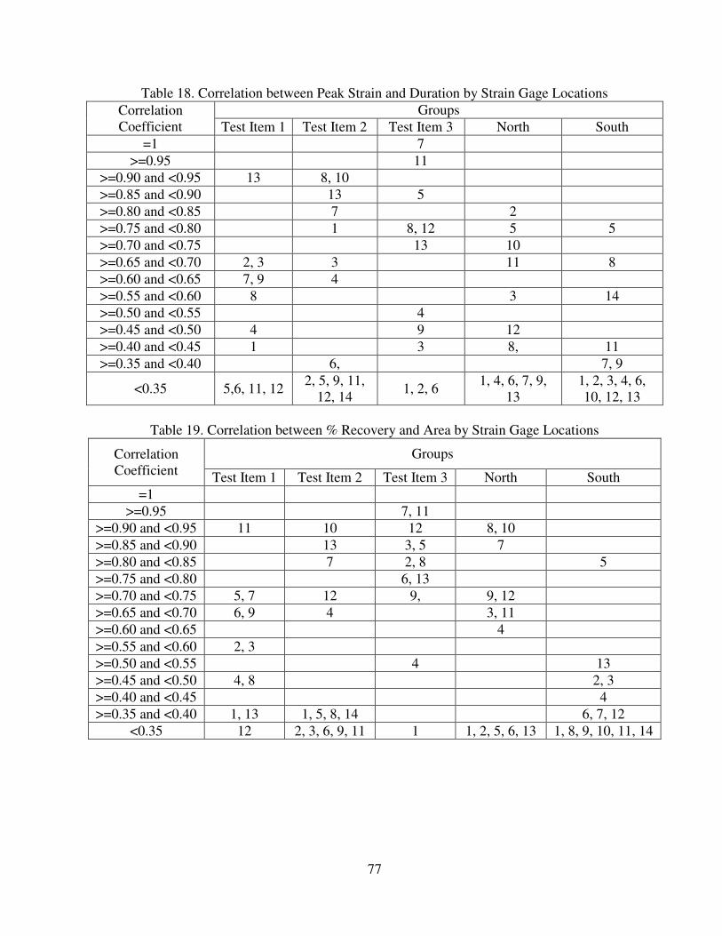
77
Table 18. Correlation between Peak Strain and Duration by Strain Gage Locations
Correlation
Coefficient
Groups
Test Item 1 Test Item 2 Test Item 3 North South
=1 7
>=0.95 11
>=0.90 and <0.95 13 8, 10
>=0.85 and <0.90 13 5
>=0.80 and <0.85 7 2
>=0.75 and <0.80 1 8, 12 5 5
>=0.70 and <0.75 13 10
>=0.65 and <0.70 2, 3 3 11 8
>=0.60 and <0.65 7, 9 4
>=0.55 and <0.60 8 3 14
>=0.50 and <0.55 4
>=0.45 and <0.50 4 9 12
>=0.40 and <0.45 1 3 8, 11
>=0.35 and <0.40 6, 7, 9
<0.35 5,6, 11, 12 2, 5, 9, 11,
12, 14 1, 2, 6
1, 4, 6, 7, 9,
13
1, 2, 3, 4, 6,
10, 12, 13
Table 19. Correlation between % Recovery and Area by Strain Gage Locations
Correlation
Coefficient
Groups
Test Item 1 Test Item 2 Test Item 3 North South
=1
>=0.95 7, 11
>=0.90 and <0.95 11 10 12 8, 10
>=0.85 and <0.90 13 3, 5 7
>=0.80 and <0.85 7 2, 8 5
>=0.75 and <0.80 6, 13
>=0.70 and <0.75 5, 7 12 9, 9, 12
>=0.65 and <0.70 6, 9 4 3, 11
>=0.60 and <0.65 4
>=0.55 and <0.60 2, 3
>=0.50 and <0.55 4 13
>=0.45 and <0.50 4, 8 2, 3
>=0.40 and <0.45 4
>=0.35 and <0.40 1, 13 1, 5, 8, 14 6, 7, 12
<0.35 12 2, 3, 6, 9, 11 1 1, 2, 5, 6, 13 1, 8, 9, 10, 11, 14
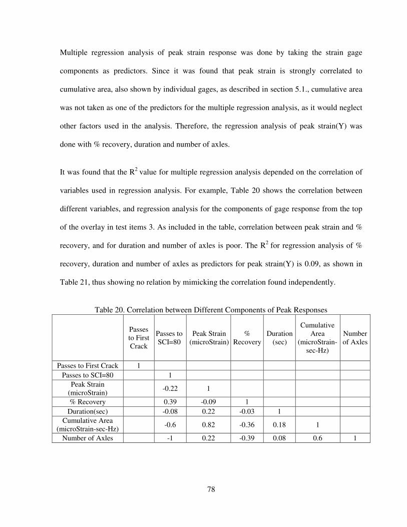
78
Multiple regression analysis of peak strain response was done by taking the strain gage
components as predictors. Since it was found that peak strain is strongly correlated to
cumulative area, also shown by individual gages, as described in section 5.1., cumulative area
was not taken as one of the predictors for the multiple regression analysis, as it would neglect
other factors used in the analysis. Therefore, the regression analysis of peak strain(Y) was
done with % recovery, duration and number of axles.
It was found that the R2
value for multiple regression analysis depended on the correlation of
variables used in regression analysis. For example, Table 20 shows the correlation between
different variables, and regression analysis for the components of gage response from the top
of the overlay in test items 3. As included in the table, correlation between peak strain and %
recovery, and for duration and number of axles is poor. The R2
for regression analysis of %
recovery, duration and number of axles as predictors for peak strain(Y) is 0.09, as shown in
Table 21, thus showing no relation by mimicking the correlation found independently.
Table 20. Correlation between Different Components of Peak Responses
Passes
to First
Crack
Passes to
SCI=80 Peak Strain
(microStrain) %
Recovery
Duration
(sec)
Cumulative
Area
(microStrain-
sec-Hz)
Number
of Axles
Passes to First Crack 1
Passes to SCI=80 1 Peak Strain
(microStrain) -0.22 1
% Recovery 0.39 -0.09 1
Duration(sec) -0.08 0.22 -0.03 1 Cumulative Area
(microStrain-sec-Hz) -0.6 0.82 -0.36 0.18 1
Number of Axles -1 0.22 -0.39 0.08 0.6 1
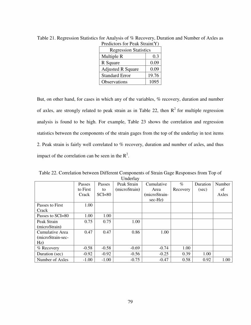
79
Table 21. Regression Statistics for Analysis of % Recovery, Duration and Number of Axles as
Predictors for Peak Strain(Y)
Regression Statistics
Multiple R 0.3
R Square 0.09
Adjusted R Square 0.09
Standard Error 19.76
Observations 1095
But, on other hand, for cases in which any of the variables, % recovery, duration and number
of axles, are strongly related to peak strain as in Table 22, then R2
for multiple regression
analysis is found to be high. For example, Table 23 shows the correlation and regression
statistics between the components of the strain gages from the top of the underlay in test items
2. Peak strain is fairly well correlated to % recovery, duration and number of axles, and thus
impact of the correlation can be seen in the R2.
Table 22. Correlation between Different Components of Strain Gage Responses from Top of
Underlay Passes
to First
Crack
Passes
to
SCI=80
Peak Strain (microStrain)
Cumulative
Area (microStrain-
sec-Hz)
%
Recovery
Duration (sec)
Number
of
Axles
Passes to First
Crack 1.00
Passes to SCI=80 1.00 1.00 Peak Strain
(microStrain) 0.75 0.75 1.00
Cumulative Area
(microStrain-sec-
Hz)
0.47 0.47 0.86 1.00
% Recovery -0.58 -0.58 -0.69 -0.74 1.00 Duration (sec) -0.92 -0.92 -0.56 -0.25 0.39 1.00 Number of Axles -1.00 -1.00 -0.75 -0.47 0.58 0.92 1.00
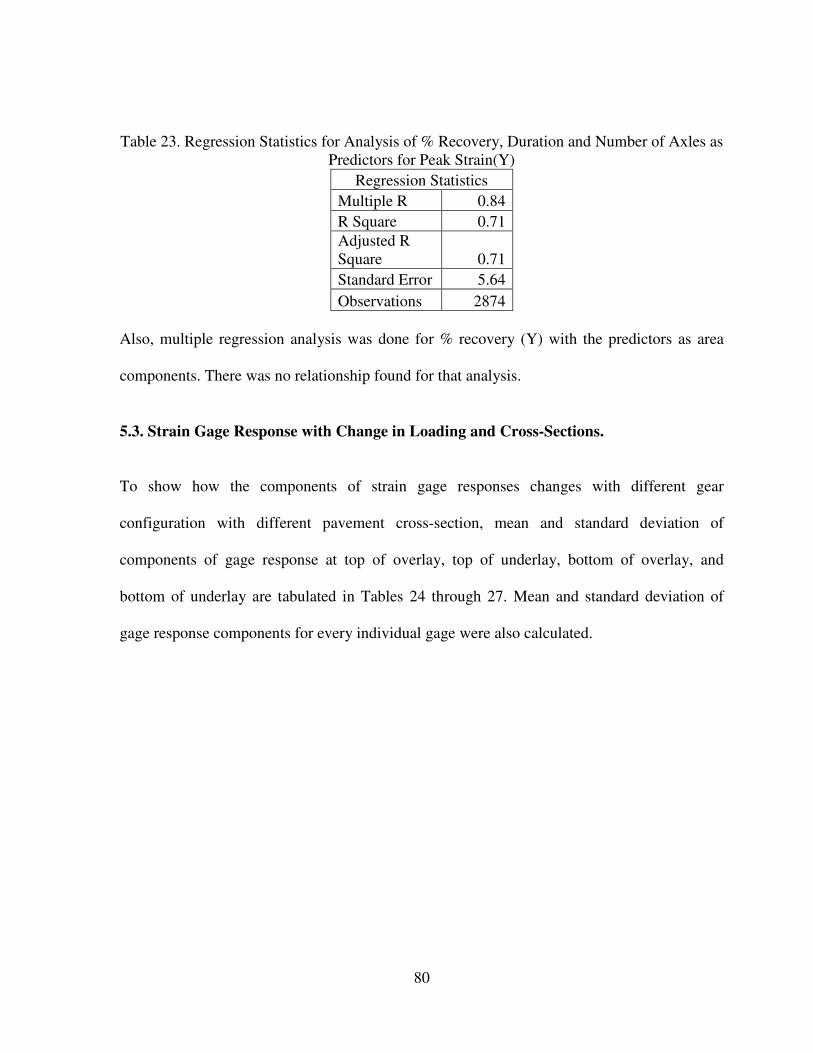
80
Table 23. Regression Statistics for Analysis of % Recovery, Duration and Number of Axles as
Predictors for Peak Strain(Y)
Regression Statistics
Multiple R 0.84
R Square 0.71
Adjusted R
Square 0.71
Standard Error 5.64
Observations 2874
Also, multiple regression analysis was done for % recovery (Y) with the predictors as area
components. There was no relationship found for that analysis.
5.3. Strain Gage Response with Change in Loading and Cross-Sections.
To show how the components of strain gage responses changes with different gear
configuration with different pavement cross-section, mean and standard deviation of
components of gage response at top of overlay, top of underlay, bottom of overlay, and
bottom of underlay are tabulated in Tables 24 through 27. Mean and standard deviation of
gage response components for every individual gage were also calculated.
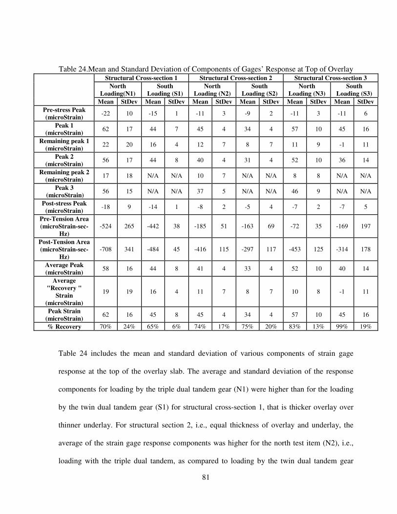
81
Table 24.Mean and Standard Deviation of Components of Gages’ Response at Top of Overlay
Structural Cross-section 1 Structural Cross-section 2 Structural Cross-section 3
North
Loading(N1)
South
Loading (S1)
North
Loading (N2)
South
Loading (S2)
North
Loading (N3)
South
Loading (S3)
Mean StDev Mean StDev Mean StDev Mean StDev Mean StDev Mean StDev
Pre-stress Peak
(microStrain) -22 10 -15 1 -11 3 -9 2 -11 3 -11 6
Peak 1
(microStrain) 62 17 44 7 45 4 34 4 57 10 45 16
Remaining peak 1
(microStrain) 22 20 16 4 12 7 8 7 11 9 -1 11
Peak 2
(microStrain) 56 17 44 8 40 4 31 4 52 10 36 14
Remaining peak 2
(microStrain) 17 18 N/A N/A 10 7 N/A N/A 8 8 N/A N/A
Peak 3
(microStrain) 56 15 N/A N/A 37 5 N/A N/A 46 9 N/A N/A
Post-stress Peak
(microStrain) -18 9 -14 1 -8 2 -5 4 -7 2 -7 5
Pre-Tension Area
(microStrain-sec-
Hz)
-524 265 -442 38 -185 51 -163 69 -72 35 -169 197
Post-Tension Area
(microStrain-sec-
Hz)
-708 341 -484 45 -416 115 -297 117 -453 125 -314 178
Average Peak
(microStrain) 58 16 44 8 41 4 33 4 52 10 40 14
Average
"Recovery "
Strain
(microStrain)
19 19 16 4 11 7 8 7 10 8 -1 11
Peak Strain
(microStrain) 62 16 45 8 45 4 34 4 57 10 45 16
% Recovery 70% 24% 65% 6% 74% 17% 75% 20% 83% 13% 99% 19%
Table 24 includes the mean and standard deviation of various components of strain gage
response at the top of the overlay slab. The average and standard deviation of the response
components for loading by the triple dual tandem gear (N1) were higher than for the loading
by the twin dual tandem gear (S1) for structural cross-section 1, that is thicker overlay over
thinner underlay. For structural section 2, i.e., equal thickness of overlay and underlay, the
average of the strain gage response components was higher for the north test item (N2), i.e.,
loading with the triple dual tandem, as compared to loading by the twin dual tandem gear
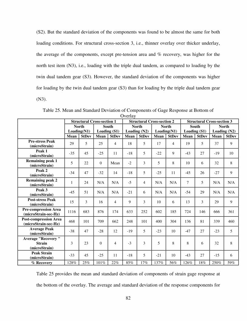
82
(S2). But the standard deviation of the components was found to be almost the same for both
loading conditions. For structural cross-section 3, i.e., thinner overlay over thicker underlay,
the average of the components, except pre-tension area and % recovery, was higher for the
north test item (N3), i.e., loading with the triple dual tandem, as compared to loading by the
twin dual tandem gear (S3). However, the standard deviation of the components was higher
for loading by the twin dual tandem gear (S3) than for loading by the triple dual tandem gear
(N3).
Table 25. Mean and Standard Deviation of Components of Gage Response at Bottom of
Overlay
Structural Cross-section 1 Structural Cross-section 2 Structural Cross-section 3
North
Loading(N1)
South
Loading (S1)
North
Loading (N2)
North
Loading(N1)
South
Loading (S1)
North
Loading (N2)
Mean StDev Mean StDev Mean StDev Mean StDev Mean StDev Mean StDev
Pre-stress Peak
(microStrain) 29 5 25 4 18 5 17 4 19 5 37 9
Peak 1
(microStrain) -35 45 -25 11 -18 5 -22 9 -43 27 -19 10
Remaining peak 1
(microStrain) 5 22 0 Mean -2 3 5 8 10 6 32 8
Peak 2
(microStrain) -34 47 -32 14 -18 5 -25 11 -45 26 -27 9
Remaining peak 2
(microStrain) 1 24 N/A N/A -5 4 N/A N/A 7 5 N/A N/A
Peak 3
(microStrain) -45 51 N/A N/A -21 6 N/A N/A -54 29 N/A N/A
Post-stress Peak
(microStrain) 15 3 16 4 9 3 10 6 13 3 29 9
Pre-compression Area
(microStrain-sec-Hz) 1116 683 876 174 633 252 602 185 724 146 666 361
Post-compression Area
(microStrain-sec-Hz) 468 101 709 662 248 101 400 304 136 81 339 460
Average Peak
(microStrain) -38 47 -28 12 -19 5 -23 10 -47 27 -23 5
Average "Recovery "
Strain
(microStrain)
3 23 0 4 -3 3 5 8 8 6 32 8
Peak Strain
(microStrain) -33 45 -25 11 -18 5 -21 10 -43 27 -15 6
% Recovery 128% 25% 101% 22% 85% 17% 137% 56% 126% 18% 250% 59%
Table 25 provides the mean and standard deviation of components of strain gage response at
the bottom of the overlay. The average and standard deviation of the response components for
83
loading with the triple dual tandem gear (N1) were higher than for the loading with the twin
dual tandem (S1) for structural cross-section 1, i.e., thicker overlay over thinner underlay
except for the post-compression area which had lower average and standard deviation for
loading by triple dual tandem. For structural cross-section 2, i.e., equal thickness of overlay
and underlay, the average of the strain gage response components was lower for north test
item (N2) , i.e., loading with triple dual tandem, as compared to loading by twin dual tandem
(S2) gear except for the pre-compression area which had higher average and standard
deviation for loading by triple dual tandem (N2). For structural cross-section 3, i.e., thinner
overlay over thicker underlay, pre-compression area showed higher mean and lower standard
deviation for north test item (N3). Post-compression area, % recovery and average peak
average “remaining” strain showed lower mean and standard deviation for north test item
(N3) than south test item (S3). Peak strain for north test item (N3) showed higher mean and
standard deviation than strain for south test item (S3).
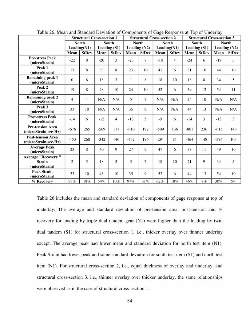
84
Table 26. Mean and Standard Deviation of Components of Gage Response at Top of Underlay
Structural Cross-section 1 Structural Cross-section 2 Structural Cross-section 3
North
Loading(N1)
South
Loading (S1)
North
Loading (N2)
North
Loading(N1)
South
Loading (S1)
North
Loading (N2)
Mean StDev Mean StDev Mean StDev Mean StDev Mean StDev Mean StDev
Pre-stress Peak
(microStrain) -22 8 -20 3 -23 7 -18 4 -24 6 -19 3
Peak 1
(microStrain) 17 8 33 8 23 10 41 6 31 10 44 10
Remaining peak 1
(microStrain) 0 6 18 3 1 8 18 10 18 8 34 5
Peak 2
(microStrain) 19 8 48 10 24 10 52 6 39 12 54 11
Remaining peak 2
(microStrain) 4 4 N/A N/A 5 7 N/A N/A 24 10 N/A N/A
Peak 3
(microStrain) 33 10 N/A N/A 35 9 N/A N/A 44 13 N/A N/A
Post-stress Peak
(microStrain) -14 6 -12 4 -13 5 -9 6 -14 3 -13 3
Pre-tension Area
(microStrain-sec-Hz) -676 265 -569 117 -610 192 -509 136 -801 236 -615 146
Post-tension Area
(microStrain-sec-Hz) -453 268 -342 146 -432 196 -291 81 -464 148 -394 103
Average Peak
(microStrain) 23 8 40 9 27 9 47 6 38 11 49 10
Average "Recovery "
Strain
(microStrain)
2 5 18 3 3 7 18 10 21 9 34 5
Peak Strain
(microStrain) 33 10 48 10 35 9 52 6 44 13 54 10
% Recovery 95% 18% 54% 10% 97% 31% 62% 18% 46% 8% 30% 6%
Table 26 includes the mean and standard deviation of components of gage response at top of
underlay. The average and standard deviation of pre-tension area, post-tension and %
recovery for loading by triple dual tandem gear (N1) were higher than the loading by twin
dual tandem (S1) for structural cross-section 1, i.e., thicker overlay over thinner underlay
except. The average peak had lower mean and standard deviation for north test item (N1).
Peak Strain had lower peak and same standard deviation for south test item (S1) and north test
item (N1). For structural cross-section 2, i.e., equal thickness of overlay and underlay, and
structural cross-section 3, i.e., thinner overlay over thicker underlay, the same relationships
were observed as in the case of structural cross-section 1.

85
Table 27. Mean and Standard Deviation of Components of Gage Response at Bottom of
Underlay
Structural Cross-section 1 Structural Cross-section 2 Structural Cross-section 3
North
Loading(N1)
South
Loading (S1)
North
Loading (N2)
North
Loading(N1)
South
Loading (S1)
North
Loading (N2)
Mean StDev Mean StDev Mean StDev Mean StDev Mean StDev Mean StDev
Pre-stress Peak
(microStrain) 17 5 16 4 23 4 17 2 13 4 16 3
Peak 1
(microStrain) -16 8 -29 13 -17 5 -28 9 -14 7 -25 3
Remaining peak 1
(microStrain) -1 6 -16 7 8 4 -8 10 -6 5 -18 1
Peak 2
(microStrain) -14 8 -32 15 -13 4 -31 11 -15 7 -28 3
Remaining peak 2
(microStrain) 0 8 N/A N/A 9 5 N/A N/A -7 5 N/A N/A
Peak 3
(microStrain) -19 10 N/A N/A -17 5 N/A N/A -16 7 N/A N/A
Post-stress Peak
(microStrain) 9 3 10 4 16 3 12 7 8 2 10 2
Pre-compression Area
(microStrain-sec-Hz) 284 191 304 132 432 135 432 120 341 139 394 117
Post-compression Area
(microStrain-sec-Hz) 523 386 496 179 668 227 535 127 440 156 542 167
Average Peak
(microStrain) -16 8 -31 14 -16 4 -30 10 -15 7 -26 2
Average "Recovery "
Strain
(microStrain)
0 7 -16 7 9 4 -8 10 -7 4 -18 1
Peak Strain
(microStrain) -12 7 -29 14 -13 4 -28 9 -13 6 -25 2
% Recovery 124% 64% 48% 6% 162% 36% 78% 27% 59% 12% 30% 5%
In Table 27, for gages at bottom of underlay the average and standard deviation of post-
compression area and % recovery for loading by triple dual tandem gear (N1) were higher
than the loading by twin dual tandem (S1) for structural cross-section 1, i.e., thicker overlay
over thinner underlay. The average and standard deviation of average peak, average
“remaining” strain and peak strain for loading by triple dual tandem gear (N1) were lower
than the loading by twin dual tandem (S1) for a structural cross-section 1. For structural cross-
section 1, a lower average and higher standard deviation for pre-compression area were
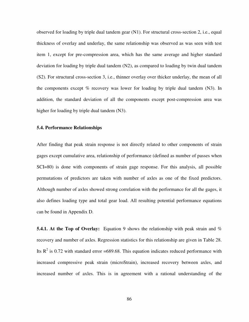
86
observed for loading by triple dual tandem gear (N1). For structural cross-section 2, i.e., equal
thickness of overlay and underlay, the same relationship was observed as was seen with test
item 1, except for pre-compression area, which has the same average and higher standard
deviation for loading by triple dual tandem (N2), as compared to loading by twin dual tandem
(S2). For structural cross-section 3, i.e., thinner overlay over thicker underlay, the mean of all
the components except % recovery was lower for loading by triple dual tandem (N3). In
addition, the standard deviation of all the components except post-compression area was
higher for loading by triple dual tandem (N3).
5.4. Performance Relationships
After finding that peak strain response is not directly related to other components of strain
gages except cumulative area, relationship of performance (defined as number of passes when
SCI=80) is done with components of strain gage response. For this analysis, all possible
permutations of predictors are taken with number of axles as one of the fixed predictors.
Although number of axles showed strong correlation with the performance for all the gages, it
also defines loading type and total gear load. All resulting potential performance equations
can be found in Appendix D.
5.4.1. At the Top of Overlay: Equation 9 shows the relationship with peak strain and %
recovery and number of axles. Regression statistics for this relationship are given in Table 28.
Its R2 is 0.72 with standard error =689.68. This equation indicates reduced performance with
increased compressive peak strain (microStrain), increased recovery between axles, and
increased number of axles. This is in agreement with a rational understanding of the
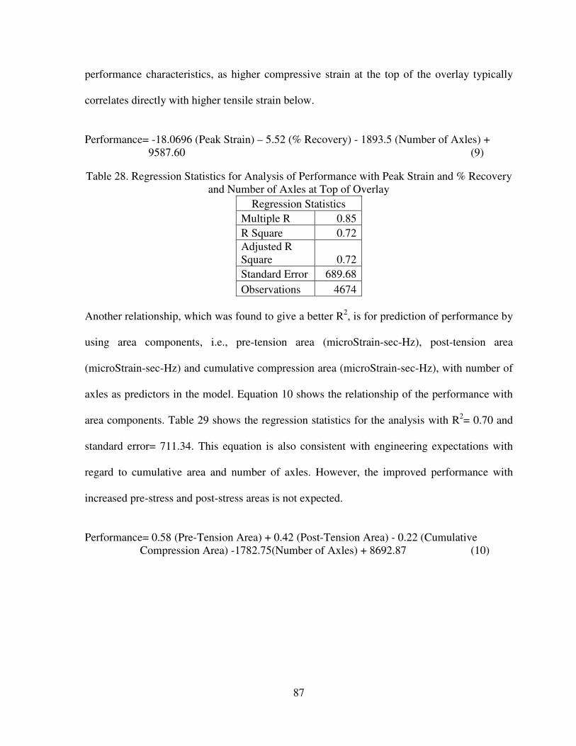
87
performance characteristics, as higher compressive strain at the top of the overlay typically
correlates directly with higher tensile strain below.
Performance= -18.0696 (Peak Strain) – 5.52 (% Recovery) - 1893.5 (Number of Axles) +
9587.60 (9)
Table 28. Regression Statistics for Analysis of Performance with Peak Strain and % Recovery
and Number of Axles at Top of Overlay
Regression Statistics
Multiple R 0.85
R Square 0.72
Adjusted R
Square 0.72
Standard Error 689.68
Observations 4674
Another relationship, which was found to give a better R2, is for prediction of performance by
using area components, i.e., pre-tension area (microStrain-sec-Hz), post-tension area
(microStrain-sec-Hz) and cumulative compression area (microStrain-sec-Hz), with number of
axles as predictors in the model. Equation 10 shows the relationship of the performance with
area components. Table 29 shows the regression statistics for the analysis with R2= 0.70 and
standard error= 711.34. This equation is also consistent with engineering expectations with
regard to cumulative area and number of axles. However, the improved performance with
increased pre-stress and post-stress areas is not expected.
Performance= 0.58 (Pre-Tension Area) + 0.42 (Post-Tension Area) - 0.22 (Cumulative
Compression Area) -1782.75(Number of Axles) + 8692.87 (10)

88
Table 29. Regression Statistics for Analysis of Performance with Pre-Tension area, Post-
Tension Area, Cumulative Compression Area and Number of Axles at Top of Overlay
Regression Statistics
Multiple R 0.84
R Square 0.70
Adjusted R
Square 0.70
Standard Error 711.34
Observations 4674
5.4.2. At the Bottom of Overlay: No rational regression relationship could be obtained for
performance by the predictors - peak strain (microStrain), % recovery and number of axles.
This is unexpected, as peak tensile strain at the bottom of the overlay would be expected by
mechanics to have the strongest negative influence on performance. However, the regression
equations developed showed improved performance with increased peak tensile strain. A
reasonable R2 is found for prediction of performance by using area components, i.e., pre-
compression area (microStrain-sec-Hz), post-compression area (microStrain-sec-Hz) and
cumulative tension area (microStrain-sec-Hz), with number of axles as predictors in the
model. Equation 11 shows the relationship of the performance with area components. Table
30 shows the regression statistics for the analysis with R2= 0.68 and standard error= 717.60.
However, this relationship also shows improved performance with increased cumulative
tensile strain area, although this is more than offset by the decreased performance with the
compression areas.
Performance= -0.05 (Pre-Compression Area) -0.41(Post-Compression Area) + 0.005
(Cumulative Tension Area) -2193.49(Number of Axles) + 9240.2 (11)
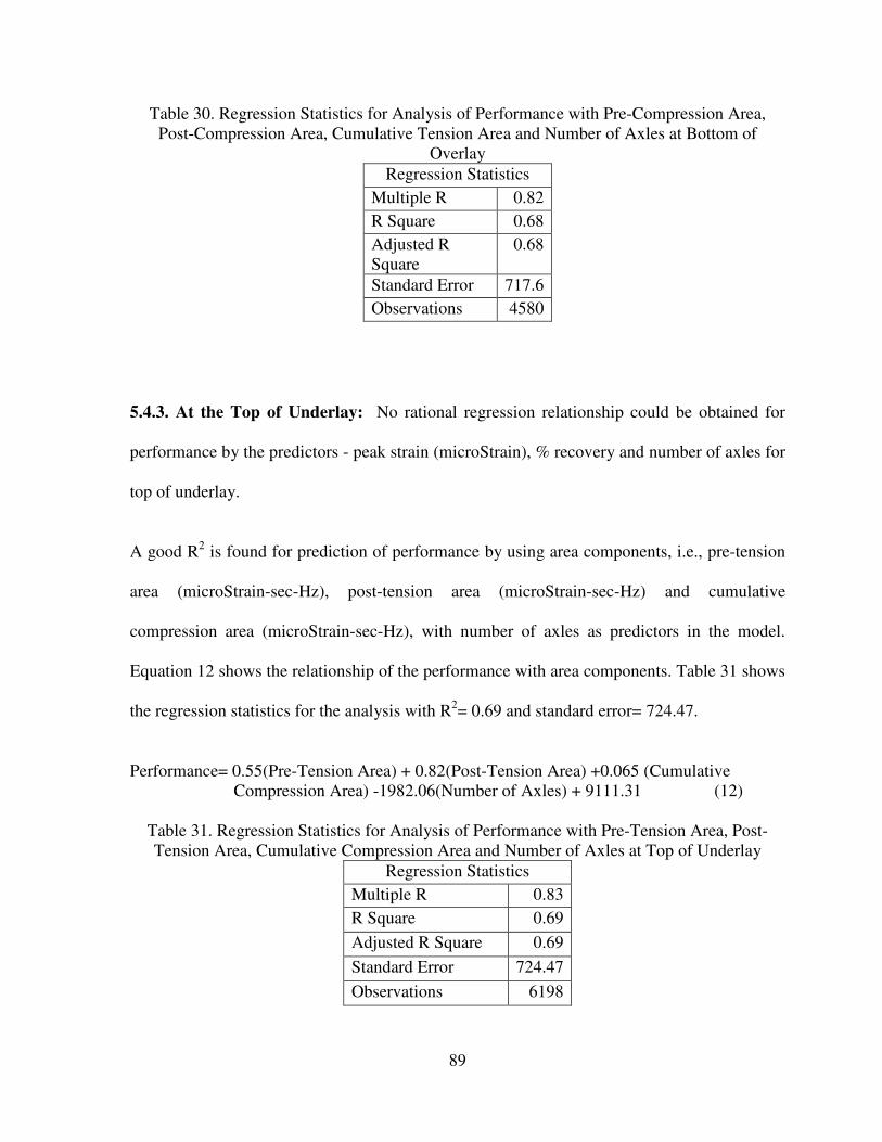
89
Table 30. Regression Statistics for Analysis of Performance with Pre-Compression Area,
Post-Compression Area, Cumulative Tension Area and Number of Axles at Bottom of
Overlay
Regression Statistics
Multiple R 0.82
R Square 0.68
Adjusted R
Square
0.68
Standard Error 717.6
Observations 4580
5.4.3. At the Top of Underlay: No rational regression relationship could be obtained for
performance by the predictors - peak strain (microStrain), % recovery and number of axles for
top of underlay.
A good R2 is found for prediction of performance by using area components, i.e., pre-tension
area (microStrain-sec-Hz), post-tension area (microStrain-sec-Hz) and cumulative
compression area (microStrain-sec-Hz), with number of axles as predictors in the model.
Equation 12 shows the relationship of the performance with area components. Table 31 shows
the regression statistics for the analysis with R2= 0.69 and standard error= 724.47.
Performance= 0.55(Pre-Tension Area) + 0.82(Post-Tension Area) +0.065 (Cumulative
Compression Area) -1982.06(Number of Axles) + 9111.31 (12)
Table 31. Regression Statistics for Analysis of Performance with Pre-Tension Area, Post-
Tension Area, Cumulative Compression Area and Number of Axles at Top of Underlay
Regression Statistics
Multiple R 0.83
R Square 0.69
Adjusted R Square 0.69
Standard Error 724.47
Observations 6198

90
5.4.4. At the Bottom of Underlay: No clearly rational relationship could be obtained for
performance by the predictors of peak strain (microStrain), % recovery and number of axles.
However, the developed equation is shown as equation 13. Regression statistics for this
relationship are given in Table 32. Its R-sq is 0.69 with standard error =706.53. This
relationship indicates decreased performance with higher peak strain and great number of
axles, as anticipated. However, the relationship also shows improved performance with
increased percent recovery. While not anticipated, the higher percent recovery may be
correlated with other parameters, such as structural cross-section, Further investigation is
warranted.
Performance= -23.5 1(Peak Strain) + 7.63 (% Recovery) - 2059.42(Number of Axles) +
7664.72 (13)
Table 32. Regression Statistics for Analysis of Performance with Peak Strain and % Recovery
and Number of Axles at Bottom of Underlay
Regression Statistics
Multiple R 0.83
R Square 0.69
Adjusted R
Square 0.69
Standard Error 706.53
Observations 6013.00
A reasonable R2 is found for prediction of performance by using area components, i.e., pre-
compression area (microStrain-sec-Hz), post-compression area (microStrain-sec-Hz) and
cumulative tension area (microStrain-sec-Hz), with number of axles as predictors in the
model. Equation 14 shows the relationship of the performance with area components. Table
32 shows the regression statistics for the analysis with R2= 0.62 and standard error= 779.28.
However, this relationship again shows improved performance with increased cumulative
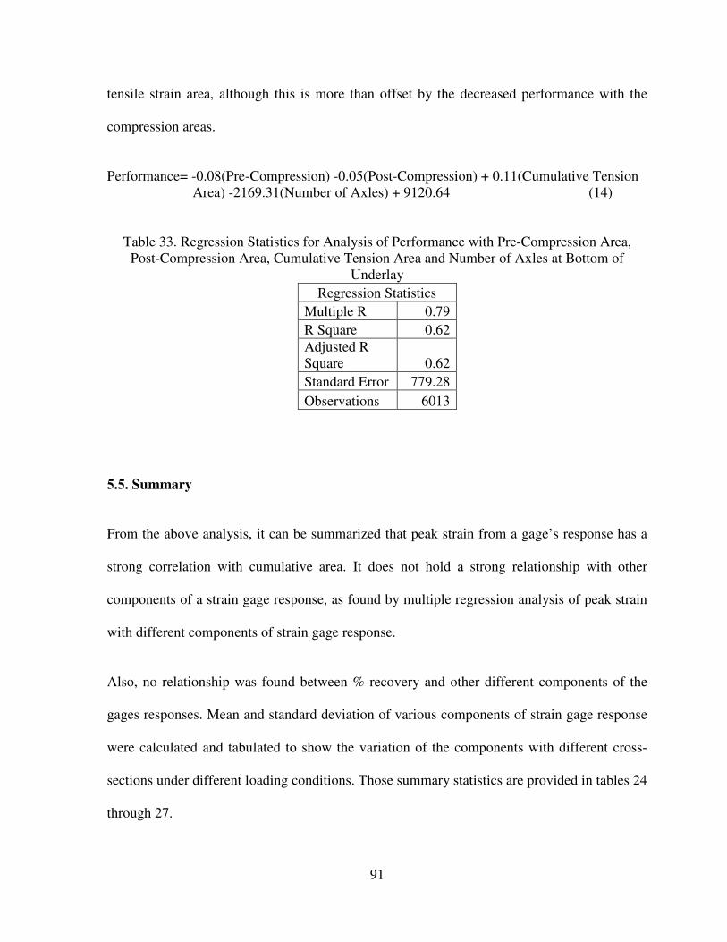
91
tensile strain area, although this is more than offset by the decreased performance with the
compression areas.
Performance= -0.08(Pre-Compression) -0.05(Post-Compression) + 0.11(Cumulative Tension
Area) -2169.31(Number of Axles) + 9120.64 (14)
Table 33. Regression Statistics for Analysis of Performance with Pre-Compression Area,
Post-Compression Area, Cumulative Tension Area and Number of Axles at Bottom of
Underlay
Regression Statistics
Multiple R 0.79
R Square 0.62
Adjusted R
Square 0.62
Standard Error 779.28
Observations 6013
5.5. Summary
From the above analysis, it can be summarized that peak strain from a gage’s response has a
strong correlation with cumulative area. It does not hold a strong relationship with other
components of a strain gage response, as found by multiple regression analysis of peak strain
with different components of strain gage response.
Also, no relationship was found between % recovery and other different components of the
gages responses. Mean and standard deviation of various components of strain gage response
were calculated and tabulated to show the variation of the components with different cross-
sections under different loading conditions. Those summary statistics are provided in tables 24
through 27.

92
Performance relationships were established, with different components of the strain gage
response and number of axles as one of the fixed predictors in the relationship. It was found
that performance has the strongest relationship with the predictors of peak strain, % recovery
and number of axles. Performance also showed relationships with different area components,
such as cumulative area, pre-strain and post-strain area, and number of axles. However, the
relationships, especially with peak tensile strain, did not always follow the rational pattern
anticipated by mechanics.
93
CHAPTER 6. CONCLUSIONS AND RECOMMENDATIONS
6.1. Findings
This study focuses on the characterization of the strain gage response. It also addresses the
relationships of peak strain response with different components of strain gage response.
Preliminary analysis of unbonded concrete overlay performance is also attempted using the
components of strain gage response.
In chapter 5, different components of the strain gage responses were compared and analyzed
for the three unbonded concrete overlay structural cross-sections and two loading conditions,
triple dual tandem and twin dual tandem. The following are the findings of that analysis:
• For each and every gage, peak strain and cumulative area show a similar trend with
change in number of passes, for constant speed of loading.
• Peak strain and cumulative area show strong correlation for all test items and south
loading conditions for gages at top of overlay, bottom of overlay, top of underlay and
bottom of underlay. Correlation coefficients range between 0.95 and 0.85 for all
loading conditions and test items analyzed here, except for gages at the top of overlay
and underlay for test item 3 as shown in Table 14.
• Since the loading speed was constant, there was no correlation found between peak
strain and duration. Hence under constant speed conditions, duration did not provide
any further information beyond what could be found from the peak strain.

94
• Correlation between % recovery and cumulative area was found to vary within a wide
range, from as low as 0.05 to as high as 0.85. Groups by loading condition show low
correlation as compared to groups characterized by cross-sections.
• Means and standard deviations for key components of stain gage response are shown
in Table 34.
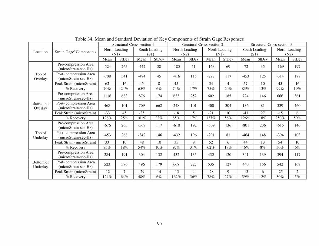
95
Table 34. Mean and Standard Deviation of Key Components of Strain Gage Responses
Location Strain Gage' Components
Structural Cross-section 1 Structural Cross-section 2 Structural Cross-section 3
North Loading
(N1)
South Loading
(S1)
North Loading
(N2)
North Loading
(N1)
South Loading
(S1)
North Loading
(N2)
Mean StDev Mean StDev Mean StDev Mean StDev Mean StDev Mean StDev
Top of
Overlay
Pre-compression Area
(microStrain-sec-Hz) -524 265 -442 38 -185 51 -163 69 -72 35 -169 197
Post- compression Area
(microStrain-sec-Hz) -708 341 -484 45 -416 115 -297 117 -453 125 -314 178
Peak Strain (microStrain) 62 16 45 8 45 4 34 4 57 10 45 16
% Recovery 70% 24% 65% 6% 74% 17% 75% 20% 83% 13% 99% 19%
Bottom of
Overlay
Pre-compression Area
(microStrain-sec-Hz) 1116 683 876 174 633 252 602 185 724 146 666 361
Post- compression Area
(microStrain-sec-Hz) 468 101 709 662 248 101 400 304 136 81 339 460
Peak Strain (microStrain) -33 45 -25 11 -18 5 -21 10 -43 27 -15 6
% Recovery 128% 25% 101% 22% 85% 17% 137% 56% 126% 18% 250% 59%
Top of
Underlay
Pre-compression Area
(microStrain-sec-Hz) -676 265 -569 117 -610 192 -509 136 -801 236 -615 146
Post- compression Area
(microStrain-sec-Hz) -453 268 -342 146 -432 196 -291 81 -464 148 -394 103
Peak Strain (microStrain) 33 10 48 10 35 9 52 6 44 13 54 10
% Recovery 95% 18% 54% 10% 97% 31% 62% 18% 46% 8% 30% 6%
Bottom of
Underlay
Pre-compression Area
(microStrain-sec-Hz) 284 191 304 132 432 135 432 120 341 139 394 117
Post- compression Area
(microStrain-sec-Hz) 523 386 496 179 668 227 535 127 440 156 542 167
Peak Strain (microStrain) -12 7 -29 14 -13 4 -28 9 -13 6 -25 2
% Recovery 124% 64% 48% 6% 162% 36% 78% 27% 59% 12% 30% 5%

96
• Performance defined as number of passes when SCI=80 is analyzed by relating it
with components of strain gage response. Performance has the strong relationship
with the predictors as peak strain and % recovery and number of axles only for
gages at the top of overlay, and the other sets of predictors as the area components
and the number of axles. R2 values for analysis done for the gages at the top of
overlay, bottom of overlay, top of underlay and bottom of underlay range between
0.62 and 0.72, with the adjusted R2 ranging from 0.62 to 0.72
6.2. Conclusions
Three questions were formulated to convey the objectives of the research. These
questions are answered as follows:
Do the various components of the strain gage response such as peaks, recovery, duration
and area directly relate to the peak strain?
From the analysis and the findings, it can be concluded that peak strain holds a strong
relationship with cumulative area. Doing analysis for each and every gage, it was found
that peak strain and cumulative area show the same trend with change in passes, with the
mean, median and standard deviation ratio of the peak strain and cumulative area to be
same. This type was expected for the loading direction as speed of a vehicle was
constant. Therefore it can be concluded, since the speed and loading of the vehicles was
constant for a particular gage, that cumulative area is a representative of a peak strain for
this particular experiment.

97
But peak strain did not show the same strong relationship with other components of the
gage responses. This implies that if other components of response may have a strong
influence on the fatigue or cracking behavior of the concrete pavement, then they must be
considered independently under this type of loading. The peak strain would not then
serve as an adequate proxy even with calibration.
As expected, the cumulative area did not show good correlation with strain gage response
components except to the peak strain. In general, cumulative area showed the same
behavior as the peak strain. Though the cumulative area represented duration of loading,
recovery between axles and strain responses due to axle loadings, it did not share any
strong relation with the components individually. This was expected because of the high
influence of peak strain on the cumulative area. Since duration depended on the speed of
loading, it was expected and observed that the duration did not show any relation with
peak strain.
How do the components of strain gage response change with different gear
configurations and different pavement cross-sections?
Mean and standard deviation for different components were obtained for each structural
cross-section (the numbered test items) at both loading conditions. It was observed that
peak strain, % recovery, average peak and pre-stress area and post-stress area show
changes as observed in Table 33 with change in the cross-section and loading conditions.

98
Though the loading by an axle is the same for different gear configurations, average peak
and recovery for a test item showed different average and standard deviation for loading
by the triple dual tandem gear and the twin dual tandem gear.
If not directly related to peak strain, how do the components of the strain gage response
relate to number of passes before cracking?
As anticipated for the small number of test items, only a preliminary answer to this
question could be obtained. Conducting multiple regression analysis, relation of the
observed performance, defined as passes to SCI=80, with the area components and the
number of axles was predicted. Performance could be predicted using peak strain and
percent recovery and number of axles for top of the overlay only. From this, it can be
concluded that performance of the pavement is dependent on area components and the
peak components.
The strain gages were installed at what were anticipated by accepted models to be the
critical locations for tensile strains that would result in transverse bottom-up cracking.
However, observed cracking patterns on the pavement were predominantly longitudinal,
and a mix of top-down and bottom-up cracking. Therefore, the strain gages were not
found to be installed at the what would have been the critical locations for the particular
experiment. This may partially explain some of the unexpected regression relationships.
It also illustrates one of the key problems with instrumented pavement designs for which
the behavior is not fully understood. Of course, those are the pavement sections from
which the most knowledge may be gained by utilizing instrumentation.
99
6.3. Recommendations
For this research, baseline experiment data from the unbonded concrete overlay
experiment at the NAPTF was used and strain responses were characterized for three
different unbonded concrete overlay cross-sections and for two different loading
conditions. Results were limited to those particular sets of data, and to the particular
locations of these strain gages, which may not have been at the most critical locations or
orientations. However, this research builds a foundation for the future work and
recommendations.
Data used in this work was simulated using two gear configurations on three structural
cross-sections. The gear configurations did not exactly reflect real aircraft, and were
limited to only twin dual tandem and triple dual tandem with each wheel load being
50,000 lbs. In order to show more varied relations, responses from real in-service aircraft
gears with varied loading conditions could be used to capture responses on other concrete
pavement structures. The FAA has instrumented concrete pavements; data from the
Denver International Airport is available.
Also, responses used in the datasets were limited to those before the first crack was
developed. Responses with the change in SCI value could also be analyzed to study
changes in response components with crack generation. After the Baseline Experiment
was over, the overlay was removed leaving the deteriorated underlay in place. A new
concrete overlay was placed over the undisturbed underlay. This study could also be
extended to the weakened support conditions in that study.

100
Perhaps the most significant conclusion of this research is that peak strain did not serve
as a full representation of strain gage response for these complex loading and structural
conditions. In addition, the preliminary statistical relationships with performance
indicated that other variables, such as % recovery between axles, may be important. This
study limited scope to the statistical characterization of the strain responses. Other
analytical approaches such as Finite Element Method and Artificial Intelligence should
be undertaken to analyze the effects of the responses. Those approaches may help to
develop future design procedures that include additional important components of
response to complex loads, instead of limiting use to only peak strain behavior.
101
REFERENCES
ACI (1992), State of the Art Report on High Strength Concrete, ACI Report 363R-92,
American Concrete Institute, Farmington Hills, Michigan, p 1-55.
Al-Qadi, I. L., Nassar, W. M., Loulizi, A., Flintsch, G. W., and Freeman, T. E. (2000),
“Flexible Pavement Instrumentation at the Virginia Smart Road,” CD-ROM Proceedings
of the 79th Annual Meeting of Transportation Research Board, Washington, D.C.
Boltz, D.E. (1998), Early Performance of Concrete Pavement containing Ground
Granulated Blast Furnace Slag, Thesis, Master of Science, Ohio University, Athens,
Ohio.
Croney M. D. and Croney P. (1998). Design & Performance of Road Pavements, 3rd
Edition, McGraw-Hill, New York.
Chou C. and Wang S. (2005), “The Analysis of Strain Data of The Monitoring System in
The Chiang-Kai-Shek International Airport,” Journal of the Eastern Asia Society for
Transportation Studies, Vol. 6, pp. 1168 – 1183.
Darestani M.Y. (2007), Response Of Concrete Pavements Under Moving Vehicular
Loads And Environmental Effects, unpublished doctorate dissertation, Queensland
University of Technology.
102
Darter, M. I., and E. J. Barenberg (1976), Zero-Maintenance Pavements. Results of Field
Studies on the Performance Requirements and Capabilities of Conventional Pavement
Systems, Report FHWA-RD-76- 105, FHWA, U.S. Department of Transportation.
Darter, M. I., and E. J. Barenberg, (1977) Design of Zero-Maintenance Plain Jointed
Concrete Pavement, Volume 1—Development of Design Procedures, Report FHWA-RD-
77-111, FHWA, U.S. Department of Transportation.
FAA (2008), Airport Improvement Program Fiscal Year 2008, Report to Congress, 25th
Annual Report of Accomplishments. Available at http://www.faa.gov/airports/aip/
grant_histories/media/aip_annual_report_fy2008.pdf
Foxworthy, P. T. (1985), Concepts for the Development of a Nondestructive Testing and
Evaluation System for Rigid Airfield Pavements, Ph. D. Dissertation, University of
Illinois, Urbana, IL, 1985.
Gaedicke C., Roesler J. and Shah S. (2009), “Fatigue crack growth prediction in concrete
slabs,” International Journal of Fatigue, No 31, p 1309–1317.
Gokhale, S., Byron, T., Iyer, S., and Choubane, B.(2009), “Evaluation of Pavement Strain
Gauge Repeatability, Results from Accelerated Pavement Testing,” Transportation
Research Record: Journal of the Transportation Research Board, No. 2094,
Transportation Research Board of the National Academies, Washington, D.C., 2009, pp.
30–40.
103
Gopalakrishnan, K., Thompson, M.R. (2006), “Effect of Dynamic Aircraft Gear Loads on
Asphalt Concrete Strain Responses,” Journal of ASTM International, Vol. 3, No. 8, p 17.
Greene J, Shahin M. Y., Alexander D. R., (2004), “Airfield pavement condition
assessment,” Transportation research record, No 1889, p 159.
Guo, E. H., Hayhoe, G. F. and Brill, D. R. (2002), “Analysis of NAPTF traffic test data
for first-year rigid pavement test items,” FAA Airport Technology Transfer Conference,
2002.
Hiller J.E., and Roesler J.R. (2005), “Determination of Critical Concrete Pavement
Fatigue Damage Locations Using Influence Lines,” Journal of Transportation
Engineering, Vol. 131, No. 8, p 599–607.
HoSang V.A. (1975), Field Survey and Analysis of Aircraft Distribution on Airport
Pavements, Report No. FAA-RD-74-36, US Department of Transportation, Federal
Aviation Administration.
Hossain A. B., Pease B., and Weiss J. (2003), “Quantifying Early-Age Stress
Development and Cracking in Low Water-to-Cement Concrete,” Transportation
Research Board. Journal of Concrete Material and construction, No. 1834.
Ioannides A.M., Thompson M.R. and Barenberg E.J. (1985), “Westergaard Solutions
Reconsidered,” Transportation Research Record 1043.

104
Khoon C.W., Meng C.C.(2005), “Airport Pavement Design and Valuation. Introduction
of Boeing 777 and Airbus A-380,” Jurutera, Nov edition, pp. 14-19.
KM Strain transducers manual, 2010, KM Strain Transducer, Available:
http://www.hoskin.qc.ca/uploadpdf/Instrumentation/TML/hoskin_EmbedmentStrainGaug
e_47cc6494078d8.pdf, April 20th
, 2010
Kohn S.D., Tayabji S.(2003), Best Practices for Airport Portland Cement Concrete
Pavement Construction (Rigid Airport Pavement), Report IPRF-01-G-002-1, An IPRF
Research Report Innovative Pavement Research Foundation Airport Concrete Pavement
Technology Program
Kuo S.S., Mahgoub H.S., and Holliday R.D. (2004), “Pavement Responses Due to Hard
Landings of Heavy Aircraft,” Transportation Research Record. Journal of the
Transportation Research Board, No. 1896, TRB, National Research Council,
Washington, D.C., pp. 88–95.
Littleton, P. (2003), Effect of Stress State on Concrete Slab Fatigue Resistance, Masters
thesis, University of Illinois, Urbana, IL.
Meyers S. L. (1951), How temperature and moisture changes may effect the durability of
concrete, Rock Products, Chicago, USA, pp. 153-157.
105
Miner, M. A. (1945), “Cumulative Damage in Fatigue,” Transactions of ASME, Journal
of Applied Mechanics, Vol. 67, p. A159.
Neville A.M. (1983), Properties of Concrete, 3rd Edition, The English Language Book
Society and Pitman Publishing, London.
Neville A.M. (1996), Properties of Concrete, 4th
and final edition, John Wiley & Sons,
Inc, New York.
Nawy E. G. (2001), Fundamentals of High-Performance Concrete, 2nd Ed.. John Wiley
& Sons Inc., New York, p.p. xiii to xvi.
Oh, B. H. (1991), “Cumulative Damage Theory of Concrete Under Variable Amplitude
Fatigue Loading,” ACI Materials Journal, Vol. 88, No. 2, pp. 41–48.
Parker, F., Barker, W.R., Gunkel, R.C., and Odom, E.C. (1979), Development of a
Structural Design Procedure for Rigid Airport Pavements, Contract No. DOT
FA73WAI-377, U.S. Army Engineer WES, Vicksburg, MS, 300 pp.
Packard, R. G. (1973), “Design of Concrete Airport Pavement,” Engineering Bulletin
EB050.03P. Portland Cement Association, Skokie, IL.
Packard, R. G. (1974), “Fatigue Concepts for Concrete Airport Pavement Design,”
Journal of Transportation Engineering, ASCE Vol. 100, No. TE3. American Society.
106
Packard, R. G. and S. D. Tayabji (1983), “Mechanistic Design of Concrete Pavements to
Control Joint Faulting and Subbase Erosion,” International Seminar on Drainage and
Erodability at the Concrete Slab-Subbase Shoulder Interface, Paris, France.
Portland Cement Association (2010), Concrete Pavements, Available.
http.//www.cement.org/pavements/pv_cp.asp, Jan 19th 2010.
Pavement Technology Advisory (2005), Unbonded Concrete Overlay, PTA-M2,
Maintenance, Repair and Rehabilitation Illinois Department of Transportation, Bureau of
Materials and Physical Research, Eff. 10/1996, Rev. 02/2005.
Ramirez F.M.Z., Thompso M. (2001), “Aircraft Multiple Wheel Gear Load Interaction
Effects on Airport Flexible Pavement Responses,” ASCE Conf. Proc. 271, 10 (2001),
DOI.10.1061/40579(271)10.
Rao S., Roesler J.R. (2004), Cumulative Fatigue Damage Analysis of Concrete Pavement
Using Accelerated Pavement Testing Results, Minnesota Department of Transportation,
Report, Submitted. 9/2/2004 2.37.49 PM GMT.
Rollings, R. (1981), “Corps of Engineers Design Procedure for Rigid Airfield
Pavements,” Proceedings of the Second International Conference on Concrete Pavement
Design, Purdue University, West Lafayette, IN, pp.185-198.
Rollings, R.S. (1986), Field Performance of Fiber Reinforced Concrete Airfield
Pavements, DOT/FAA/PM-86/26, Federal Aviation Administration, Washington, D.C.

107
Rollings, R.S. (1988), Design of Overlays for Rigid Airfield Pavements. Final Report,
DOT/FAA/PM-87/19, Federal Aviation Administration, Washington, D.C.
Rollings, R.S. and Witczak, M. (1990), “Structural Deterioration Model for Rigid
Airfield Pavements,” ASCE, Journal of Transportation Engineering, Vol. 116, No. 4, pp.
479-491.
Rollings, R.S. (2001), “Concrete Pavement Design. Its More Than a Thickness Design
Chart,” Proceedings of the Seventh International Conference on Concrete Pavement
Design, Lake Buena Vista, FL, pp.281-296.
Rollings, R.S. (1998), “Evolution of the U.S. Military’s Concrete Airfield Pavement
Design Procedures,” Proceedings, Fourth International Workshop on Design Theories
and Their Verification of Concrete Slabs for Pavements and Railroads, Bucaco,
Portugal, pp. 263-276.
Darter, M. I. (1988), A Comparison Between Corps of Engineers and ERES Consultants,
Inc. Rigid Pavement Design Procedures, Technical Report Prepared for the United States
Air Force SAC Command. Savoy, IL, 1988.
Roesler J.R. (1988), Fatigue of concrete beams and slabs, Ph.D. Thesis, University of
Illinois, Urbana, Illinois, p. 483.
108
Roesler J.R., Littleton P.C., Hiller J.E., Long G.E. (2004), Effect of stress state on
concrete slab fatigue resistance, Draft final report for Federal Aviation Administration.
Urbana, IL. University of Illinois, p. 227.
Roesler J.R., Hiller J.E., Littleton P.C. (2005), “Large-scale airfield concrete slab fatigue
tests,” Proceedings of the 8th international conference on concrete pavements, vol. 3.
Colorado Springs, CO; 2005. p. 1247–68.
Roesler J.R. (2006), “Fatigue resistance of concrete pavements,” 6th international DUT
– workshop on fundamental modelling of design and performance of concrete pavements,
Belgium.
Roesler J.R., Hiller J.E., and Littleton P.C., (2004), Large-Scale Airfield Concrete Slab
Fatigue Tests, Volume 1, Number 1, paper 5.
Roesler, J.R., and Barenberg, E.J., (1999). Effect of Static and Fatigue Cracking on
Concrete Strain Measurements, Transportation Research Record: Journal of the
Transportation Research Board, Volume 1684, p 51-60.
Salsilli, R. A., E. J. Barenberg, and M. I. Darter (1993), “Calibrated Mechanistic Design
Procedure to Prevent Transverse Cracking of Jointed Plain Concrete Pavements,”
Proceedings, 5th International Conference on Concrete Pavements, West LaFayette, IN.
109
Sebaaly, P. E., and Tabatabaee, N. (1991), “Field Evaluation of Strain Gauges in Asphalt
Concrete Pavements,” Proceedings of the Second International Symposium on Pavement
Response Monitoring Systems for Roads and Airfields, Hanover, NH.
Smith, K. and Roesler, J.R. (2003), “Review of Fatigue Models for Concrete Airfield
Pavement Design,” ASCE Airfield Pavement Specialty Conference, Las Vegas, NV,
September 21-24, pp 26.
Standard Test Method for Airport Pavement Condition Index Surveys, July 1, 2004
edition, Designation: D 5340 – 04.
Strain Gage (2010), Available:http://www.straingage.com/strain_gages/what_strain.html,
April 20, 2010.
Stoffels S., Morian D., Ioannides A., Wu S., Suri, S., Yeh L. and Yin H.(2006), Improved
Overlay Design Parameters for Concrete Airfield Pavements, Report, Innovative
Pavement Research Foundation (IPRF), Project FAA-01-G-002-04-02.
Tia M., Liu Y., and Brown D. (2005), Modulus of Elasticity, Creep and Shrinkage of
Concrete, Final Report, U.F. Project No. 49104504973-12, Contract No- BC 354,
Department of Coastal and Civil Engineering, University of Florida, Gainesville, Florida.
Tigdemir M., Karasahin M., and Sen Z. (2002), “Investigation of fatigue behaviour of
asphalt concrete pavements with fuzzy-logic approach,” International Journal of Fatigue,
No 24, p 903–910.
110
Vogelzang, C. H., and Bouman, S. R. (1991), “In Situ Stress and Strain Measurements in
Dynamically Loaded Asphalt Pavement Structures,” Proceedings of the Second
International Symposium on Pavement Response Monitoring Systems for Roads and
Airfields, Hanover.
Weinmann, T. L., Lewis, A. E., and Tayabji, S. D. (2004), “Pavement Sensors used at
Accelerated Pavement Test Facilities,” Proceedings of the Second International
Conference on Accelerated Pavement Testing, University of Minnesota, Minneapolis,
MN.
Westergaard, H.M. (1926), “Stresses in Concrete Pavements Computed by Theoretical
Analysis,” Public Roads, Vol. 7, No. 2, pp. 25-35.
Westergaard, H.M. (1948), “New Formulas for Stresses in Concrete Pavements of
Airfields,” ASCE Transactions, Vol. 113.
Yun K.K, Kim D.H., Jeong W.K., and Chimoon Won,(2005), “Comparative Study of
Cumulative Damage to Pavement Concrete Under Splitting Tensile, Variable Amplitude
Fatigue Loadings,” Transportation Research Record. Journal of the Transportation
Research Board, No. 1914, Transportation Research Board of the National Academies,
Washington, D.C., pp. 24–33.

111
APPENDIX A: Strain gage coordinates and calibration factor
Structural Cross-section 1
Table 35. Coordinates and Calibration Factor for Strain Gages Installed at Test Item N1.
Sensor Test Item Overlay/Underlay Xloc ft Yloc ft Zloc in Calibration
Factor
EG-O-N1-1 B N1 Overlay 338.75 -17.25
0.818
EG-O-N1-1 T N1 Overlay 338.75 -17.25
0.812
EG-O-N1-2 B N1 Overlay 363.75 -17.25
0.806
EG-O-N1-2 T N1 Overlay 363.75 -17.25
0.808
EG-O-N1-3 B N1 Overlay 376.25 -17.25
0.817
EG-O-N1-3 T N1 Overlay 376.25 -17.25
0.81
EG-U-N1-1 B N1 Underlay 338.75 -17.5 -5.5 0.787
EG-U-N1-1 T N1 Underlay 338.75 -17.5 -1.17 0.79
EG-U-N1-2 B N1 Underlay 366 -17.5 -5.5 0.804
EG-U-N1-2 T N1 Underlay 363.75 -17.5 -1.17 0.786
EG-U-N1-3 B N1 Underlay 370 -17.5 -5.5 0.782
EG-U-N1-3 T N1 Underlay 370 -17.5 -1.17 0.808
Table 36. Coordinates and Calibration Factor for Strain Gages Installed at Test Item S1.
Sensor Test
Item Overlay/Underlay Xloc ft Yloc ft
Zloc
in
Calibration
Factor
EG-O-S1-1 B S1 Overlay 338.75 17.25
0.814
EG-O-S1-1 T S1 Overlay 338.75 17.25
0.817
EG-O-S1-2 B S1 Overlay 363.75 17.25
0.813
EG-O-S1-2 T S1 Overlay 363.75 17.25
0.818
EG-O-S1-3 B S1 Overlay 376.25 17.25
0.808
EG-O-S1-3 T S1 Overlay 376.25 17.25
0.817
EG-U-S1-1 B S1 Underlay 338.75 17.5 -5.5 0.79
EG-U-S1-1 T S1 Underlay 338.75 17.5 -1.17 0.785
EG-U-S1-2 B S1 Underlay 366 17.5 -5.5 0.786
EG-U-S1-2 T S1 Underlay 363.75 17.5 -1.17 0.782
EG-U-S1-3 B S1 Underlay 370 17.5 -5.5 0.786
EG-U-S1-3 T S1 Underlay 370 17.5 -1.17 0.801
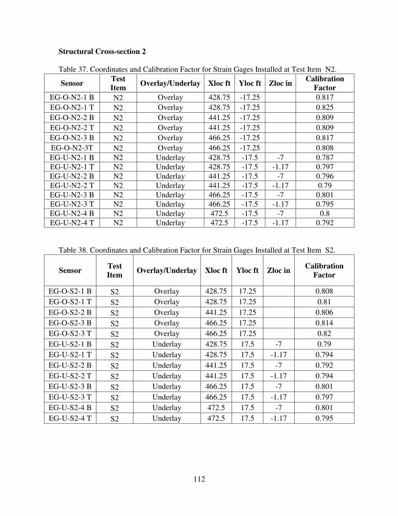
112
Structural Cross-section 2
Table 37. Coordinates and Calibration Factor for Strain Gages Installed at Test Item N2.
Sensor Test
Item Overlay/Underlay Xloc ft Yloc ft Zloc in
Calibration
Factor
EG-O-N2-1 B N2 Overlay 428.75 -17.25
0.817
EG-O-N2-1 T N2 Overlay 428.75 -17.25
0.825
EG-O-N2-2 B N2 Overlay 441.25 -17.25
0.809
EG-O-N2-2 T N2 Overlay 441.25 -17.25
0.809
EG-O-N2-3 B N2 Overlay 466.25 -17.25
0.817
EG-O-N2-3T N2 Overlay 466.25 -17.25
0.808
EG-U-N2-1 B N2 Underlay 428.75 -17.5 -7 0.787
EG-U-N2-1 T N2 Underlay 428.75 -17.5 -1.17 0.797
EG-U-N2-2 B N2 Underlay 441.25 -17.5 -7 0.796
EG-U-N2-2 T N2 Underlay 441.25 -17.5 -1.17 0.79
EG-U-N2-3 B N2 Underlay 466.25 -17.5 -7 0.801
EG-U-N2-3 T N2 Underlay 466.25 -17.5 -1.17 0.795
EG-U-N2-4 B N2 Underlay 472.5 -17.5 -7 0.8
EG-U-N2-4 T N2 Underlay 472.5 -17.5 -1.17 0.792
Table 38. Coordinates and Calibration Factor for Strain Gages Installed at Test Item S2.
Sensor Test
Item Overlay/Underlay Xloc ft Yloc ft Zloc in
Calibration
Factor
EG-O-S2-1 B S2 Overlay 428.75 17.25
0.808
EG-O-S2-1 T S2 Overlay 428.75 17.25
0.81
EG-O-S2-2 B S2 Overlay 441.25 17.25
0.806
EG-O-S2-3 B S2 Overlay 466.25 17.25
0.814
EG-O-S2-3 T S2 Overlay 466.25 17.25
0.82
EG-U-S2-1 B S2 Underlay 428.75 17.5 -7 0.79
EG-U-S2-1 T S2 Underlay 428.75 17.5 -1.17 0.794
EG-U-S2-2 B S2 Underlay 441.25 17.5 -7 0.792
EG-U-S2-2 T S2 Underlay 441.25 17.5 -1.17 0.794
EG-U-S2-3 B S2 Underlay 466.25 17.5 -7 0.801
EG-U-S2-3 T S2 Underlay 466.25 17.5 -1.17 0.797
EG-U-S2-4 B S2 Underlay 472.5 17.5 -7 0.801
EG-U-S2-4 T S2 Underlay 472.5 17.5 -1.17 0.795

113
Structural Cross-section 3
Table 39. Coordinates and Calibration Factor for Strain Gages Installed at Test Item N3.
Sensor Test
Item Overlay/Underlay Xloc ft Yloc ft Zloc in
Calibration
Factor
EG-O-N3-1 B N3 Overlay 518.75 -17.25
0.813
EG-O-N3-1 T N3 Overlay 518.75 -17.25
0.812
EG-O-N3-2 B N3 Overlay 543.75 -17.25
0.817
EG-O-N3-2 T N3 Overlay 543.75 -17.25
0.814
EG-O-N3-3 B N3 Overlay 556.25 -17.25
0.814
EG-O-N3-3 T N3 Overlay 556.25 -17.25
0.809
EG-U-N3-1 B N3 Underlay 518.75 -17.5 -9.5 0.787
EG-U-N3-1 T N3 Underlay 518.75 -17.5 -1.17 0.795
EG-U-N3-2 B N3 Underlay 546 -17.5 -9.5 0.803
EG-U-N3-2 T N3 Underlay 543.75 -17.5 -1.17 0.786
EG-U-N3-3 B N3 Underlay 550 -17.5 -9.5 0.796
EG-U-N3-3 T N3 Underlay 550 -17.5 -1.17 0.781
Table 40. Coordinates and Calibration Factor for Strain Gages Installed at Test Item S3.
Sensor Test
Item Overlay/Underlay Xloc ft Yloc ft Zloc in
Calibration
Factor
EG-O-S3-1 B S3 Overlay 518.75 17.25
0.813
EG-O-S3-1 T S3 Overlay 518.75 17.25
0.81
EG-O-S3-2 B S3 Overlay 543.75 17.25
0.812
EG-O-S3-2 T S3 Overlay 543.75 17.25
0.795
EG-O-S3-3 B S3 Overlay 556.25 17.25
0.804
EG-O-S3-3 T S3 Overlay 556.25 17.25
0.817
EG-U-S3-1 B S3 Underlay 518.75 17.5 -9.5 0.789
EG-U-S3-1 T S3 Underlay 518.75 17.5 -1.17 0.794
EG-U-S3-2 B S3 Underlay 546 17.5 -9.5 0.797
EG-U-S3-2 T S3 Underlay 543.75 17.5 -1.17 0.79
EG-U-S3-3 B S3 Underlay 550 17.5 -9.5 0.796
EG-U-S3-3 T S3 Underlay 550 17.5 -1.17 0.792
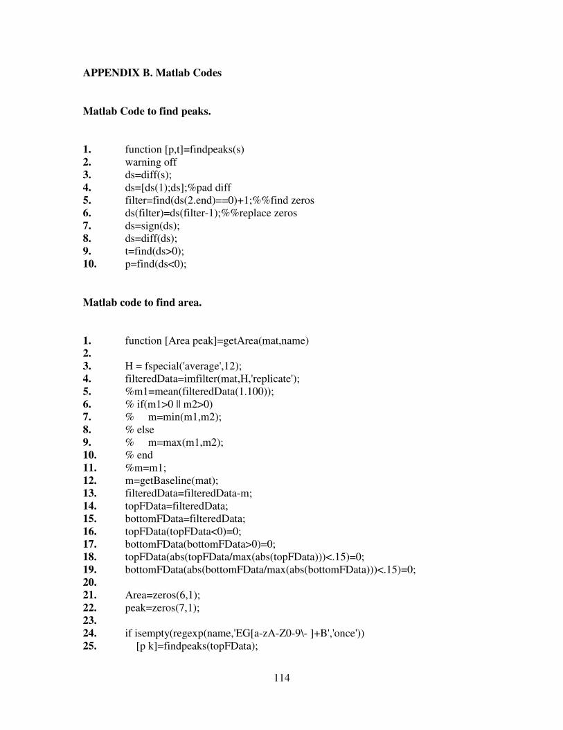
114
APPENDIX B. Matlab Codes
Matlab Code to find peaks.
1. function [p,t]=findpeaks(s)
2. warning off
3. ds=diff(s);
4. ds=[ds(1);ds];%pad diff
5. filter=find(ds(2.end)==0)+1;%%find zeros
6. ds(filter)=ds(filter-1);%%replace zeros
7. ds=sign(ds);
8. ds=diff(ds);
9. t=find(ds>0);
10. p=find(ds<0);
Matlab code to find area.
1. function [Area peak]=getArea(mat,name)
2.
3. H = fspecial('average',12);
4. filteredData=imfilter(mat,H,'replicate');
5. %m1=mean(filteredData(1.100));
6. % if(m1>0 || m2>0)
7. % m=min(m1,m2);
8. % else
9. % m=max(m1,m2);
10. % end
11. %m=m1;
12. m=getBaseline(mat);
13. filteredData=filteredData-m;
14. topFData=filteredData;
15. bottomFData=filteredData;
16. topFData(topFData<0)=0;
17. bottomFData(bottomFData>0)=0;
18. topFData(abs(topFData/max(abs(topFData)))<.15)=0;
19. bottomFData(abs(bottomFData/max(abs(bottomFData)))<.15)=0;
20.
21. Area=zeros(6,1);
22. peak=zeros(7,1);
23.
24. if isempty(regexp(name,'EG[a-zA-Z0-9\- ]+B','once'))
25. [p k]=findpeaks(topFData);
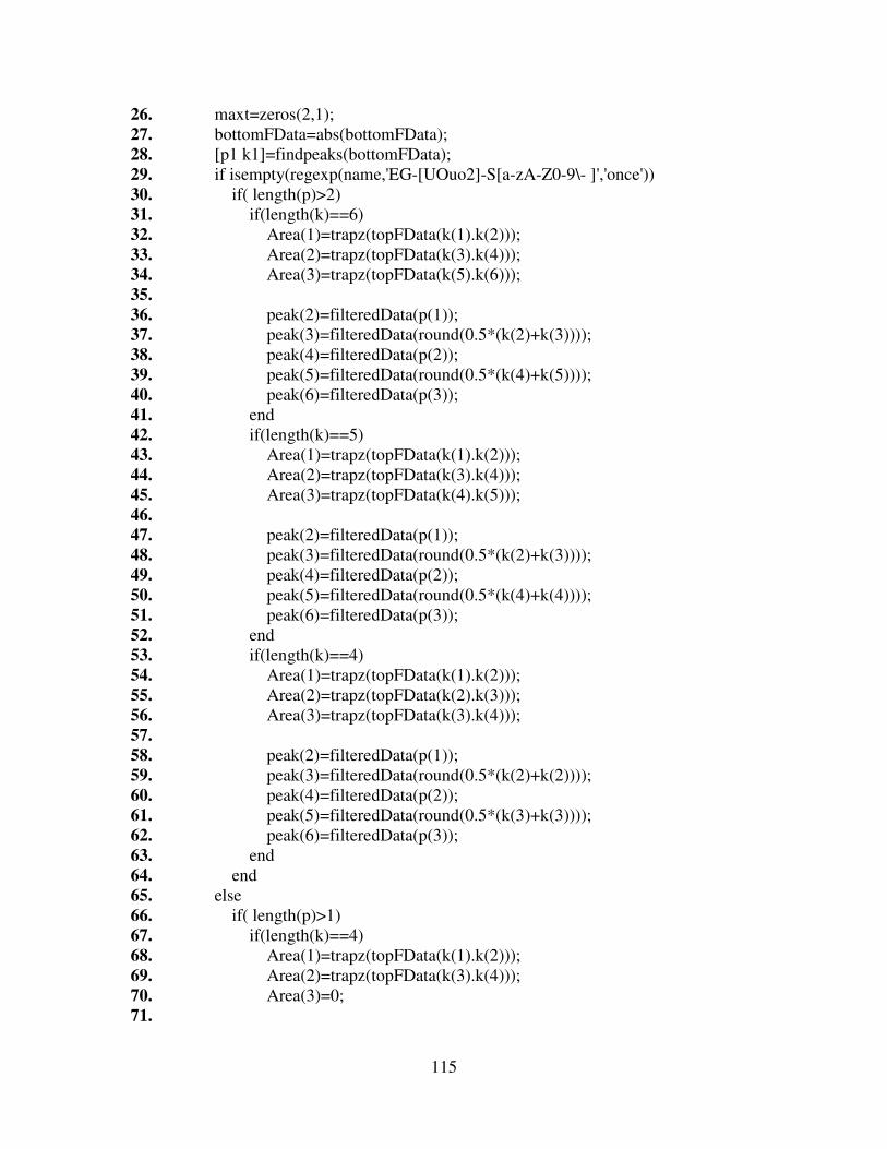
115
26. maxt=zeros(2,1);
27. bottomFData=abs(bottomFData);
28. [p1 k1]=findpeaks(bottomFData);
29. if isempty(regexp(name,'EG-[UOuo2]-S[a-zA-Z0-9\- ]','once'))
30. if( length(p)>2)
31. if(length(k)==6)
32. Area(1)=trapz(topFData(k(1).k(2)));
33. Area(2)=trapz(topFData(k(3).k(4)));
34. Area(3)=trapz(topFData(k(5).k(6)));
35.
36. peak(2)=filteredData(p(1));
37. peak(3)=filteredData(round(0.5*(k(2)+k(3))));
38. peak(4)=filteredData(p(2));
39. peak(5)=filteredData(round(0.5*(k(4)+k(5))));
40. peak(6)=filteredData(p(3));
41. end
42. if(length(k)==5)
43. Area(1)=trapz(topFData(k(1).k(2)));
44. Area(2)=trapz(topFData(k(3).k(4)));
45. Area(3)=trapz(topFData(k(4).k(5)));
46.
47. peak(2)=filteredData(p(1));
48. peak(3)=filteredData(round(0.5*(k(2)+k(3))));
49. peak(4)=filteredData(p(2));
50. peak(5)=filteredData(round(0.5*(k(4)+k(4))));
51. peak(6)=filteredData(p(3));
52. end
53. if(length(k)==4)
54. Area(1)=trapz(topFData(k(1).k(2)));
55. Area(2)=trapz(topFData(k(2).k(3)));
56. Area(3)=trapz(topFData(k(3).k(4)));
57.
58. peak(2)=filteredData(p(1));
59. peak(3)=filteredData(round(0.5*(k(2)+k(2))));
60. peak(4)=filteredData(p(2));
61. peak(5)=filteredData(round(0.5*(k(3)+k(3))));
62. peak(6)=filteredData(p(3));
63. end
64. end
65. else
66. if( length(p)>1)
67. if(length(k)==4)
68. Area(1)=trapz(topFData(k(1).k(2)));
69. Area(2)=trapz(topFData(k(3).k(4)));
70. Area(3)=0;
71.
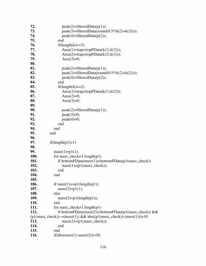
116
72. peak(2)=filteredData(p(1));
73. peak(3)=filteredData(round(0.5*(k(2)+k(3))));
74. peak(4)=filteredData(p(2));
75. end
76. if(length(k)==3)
77. Area(1)=trapz(topFData(k(1).k(2)));
78. Area(2)=trapz(topFData(k(2).k(3)));
79. Area(3)=0;
80.
81. peak(2)=filteredData(p(1));
82. peak(3)=filteredData(round(0.5*(k(2)+k(2))));
83. peak(4)=filteredData(p(2));
84. end
85. if(length(k)==2)
86. Area(1)=trapz(topFData(k(1).k(2)));
87. Area(2)=0;
88. Area(3)=0;
89.
90. peak(2)=filteredData(p(1));
91. peak(3)=0;
92. peak(4)=0;
93. end
94. end
95. end
96.
97. if(length(p1)>1)
98.
99. maxt(1)=p1(1);
100. for maxt_check=1.length(p1)
101. if bottomFData(maxt(1))<bottomFData(p1(maxt_check))
102. maxt(1)=(p1(maxt_check));
103. end
104. end
105.
106. if maxt(1)==p1(length(p1))
107. maxt(2)=p1(1);
108. else
109. maxt(2)=p1(length(p1));
110. end
111. for maxt_check=1.length(p1)
112. if bottomFData(maxt(2))<bottomFData(p1(maxt_check)) &&
(p1(maxt_check))~=(maxt(1)) && abs((p1(maxt_check))-(maxt(1)))>10
113. maxt(2)=(p1(maxt_check));
114. end
115. end
116. if(abs(maxt(1)-maxt(2))>10)
117
117. % area6 is time
118. Area(6)= abs(maxt(1)-maxt(2));
119. peak(1)=filteredData(maxt(1));
120. if isempty(regexp(name,'EG-[UOuo2]-S[a-zA-Z0-9\- ]','once'))
121. peak(7)=filteredData(maxt(2));
122. else
123. peak(5)=filteredData(maxt(2));
124. end
125.
126. if maxt(1)>maxt(2)
127. kt=maxt(2);
128. maxt(2)=maxt(1);
129. maxt(1)=kt;
130. end
131.
132. new_k1=k1(bottomFData(k1)==0);
133. % new_k1.array=[];
134. % cou=1;
135. % for c=1.length(k1)
136. % if(bottomFData(k1(c))==0)
137. % new_k1(cou)=k1(c);
138. % cou=cou+1;
139. % end
140. % end
141. if(length(new_k1)>1)
142. mp1=abs(new_k1(1)-maxt(1));
143. mp1_k1=new_k1(1);
144. for maxt_check=1.length(new_k1)
145. if mp1 > abs(new_k1(maxt_check)-maxt(1))
146. mp1_k1=new_k1(maxt_check);
147. end
148. end
149.
150. if mp1_k1==new_k1(1)
151. mp1=abs(new_k1(2)-maxt(1));
152. mp1_k2=new_k1(2);
153. else
154. mp1=abs(new_k1(1)-maxt(1));
155. mp1_k2=new_k1(1);
156. end
157. for maxt_check=1.length(new_k1)
158. if mp1 > abs(new_k1(maxt_check)-maxt(1)) &&
mp1_k1~=new_k1(maxt_check)
159. mp1_k2=new_k1(maxt_check);
160. end
161. end
118
162.
163. if(mp1_k1>mp1_k2)
164. kp=mp1_k1;
165. mp1_k1=mp1_k2;
166. mp1_k2=kp;
167. end
168. Area(4)=trapz(topFData(mp1_k1.mp1_k2));
169.
170. mp1=abs(new_k1(1)-maxt(2));
171. mp1_k1=new_k1(1);
172. for maxt_check=1.length(new_k1)
173. if mp1 > abs(new_k1(maxt_check)-maxt(2))
174. mp1_k1=new_k1(maxt_check);
175. end
176. end
177. if mp1_k1==new_k1(1)
178. mp1=abs(new_k1(2)-maxt(2));
179. mp1_k2=new_k1(2);
180. else
181. mp1=abs(new_k1(1)-maxt(2));
182. mp1_k2=new_k1(1);
183. end
184. for maxt_check=1.length(new_k1)
185. if mp1 > abs(new_k1(maxt_check)-maxt(2)) &&
mp1_k1~=new_k1(maxt_check)
186. mp1_k2=new_k1(maxt_check);
187. end
188. end
189.
190. if(mp1_k1>mp1_k2)
191. kp=mp1_k1;
192. mp1_k1=mp1_k2;
193. mp1_k2=kp;
194. end
195. Area(5)=trapz(topFData(mp1_k1.mp1_k2));
196. end
197. end
198. end
199.
200. end
201.
202.
203. if isempty(regexp(name,'EG[a-zA-Z0-9\- ]+T','once'))
204.
205. [p k]=findpeaks(bottomFData);
206. [p1 k1]=findpeaks(topFData);
119
207.
208. if isempty(regexp(name,'EG-[UOuo2]-S[a-zA-Z0-9\- ]','once'))
209. if( length(k)>2)
210. if(length(p)==6)
211. Area(1)=trapz(bottomFData(p(1).p(2)));
212. Area(2)=trapz(bottomFData(p(3).p(4)));
213. Area(3)=trapz(bottomFData(p(5).p(6)));
214.
215. peak(2)=filteredData(k(1));
216. peak(3)=filteredData(round(0.5*(p(2)+p(3))));
217. peak(4)=filteredData(k(2));
218. peak(5)=filteredData(round(0.5*(p(4)+p(5))));
219. peak(6)=filteredData(k(3));
220. end
221. if(length(p)==5)
222. Area(1)=trapz(bottomFData(p(1).p(2)));
223. Area(2)=trapz(bottomFData(p(3).p(4)));
224. Area(3)=trapz(bottomFData(p(4).p(5)));
225.
226. peak(2)=filteredData(k(1));
227. peak(3)=filteredData(round(0.5*(p(2)+p(3))));
228. peak(4)=filteredData(k(2));
229. peak(5)=filteredData(round(0.5*(p(4)+p(4))));
230. peak(6)=filteredData(k(3));
231. end
232. if(length(p)==4)
233. Area(1)=trapz(bottomFData(p(1).p(2)));
234. Area(2)=trapz(bottomFData(p(2).p(3)));
235. Area(3)=trapz(bottomFData(p(3).p(4)));
236.
237. peak(2)=filteredData(k(1));
238. peak(3)=filteredData(round(0.5*(p(2)+p(2))));
239. peak(4)=filteredData(k(2));
240. peak(5)=filteredData(round(0.5*(p(3)+p(3))));
241. peak(6)=filteredData(k(3));
242. end
243. end
244. else
245. if(length(k)>1)
246. if(length(p)==3)
247. Area(1)=trapz(bottomFData(p(1).p(2)));
248. Area(2)=trapz(bottomFData(p(2).p(3)));
249. Area(3)=0;
250.
251. peak(2)=filteredData(k(1));
252. peak(3)=filteredData(round(0.5*(p(2)+p(2))));

120
253. peak(4)=filteredData(k(2));
254. end
255. if(length(p)==2)
256. Area(1)=trapz(bottomFData(p(1).p(2)));
257. Area(2)=0;
258. Area(3)=0;
259.
260. peak(2)=filteredData(k(1));
261. peak(3)=0;
262. peak(4)=0;
263. end
264. if(length(p)==4)
265. Area(1)=trapz(bottomFData(p(1).p(2)));
266. Area(2)=trapz(bottomFData(p(3).p(4)));
267. Area(3)=0;
268.
269. peak(2)=filteredData(k(1));
270. peak(3)=filteredData(round(0.5*(p(2)+p(3))));
271. peak(4)=filteredData(k(2));
272. end
273. end
274. end
275. if(length(p1)>1)
276. maxt(1)=p1(1);
277. for maxt_check=1.length(p1)
278. if topFData(maxt(1))<topFData(p1(maxt_check))
279. maxt(1)=(p1(maxt_check));
280. end
281. end
282.
283. if maxt(1)==p1(length(p1))
284. maxt(2)=p1(1);
285. else
286. maxt(2)=p1(length(p1));
287. end
288. for maxt_check=1.length(p1)
289. if topFData(maxt(2))<topFData(p1(maxt_check)) &&
(p1(maxt_check))~=(maxt(1)) && abs((p1(maxt_check))-(maxt(1)))>10
290. maxt(2)=(p1(maxt_check));
291. end
292. end
293.
294. if(abs(maxt(1)-maxt(2))>10)
295. % area6 is time
296. Area(6)= abs(maxt(1)-maxt(2));
297. peak(1)=filteredData(maxt(1));
121
298. if isempty(regexp(name,'EG-[UOuo2]-S[a-zA-Z0-9\- ]','once'))
299. peak(7)=filteredData(maxt(2));
300. else
301. peak(5)=filteredData(maxt(2));
302. end
303.
304. if maxt(1)>maxt(2)
305. kt=maxt(2);
306. maxt(2)=maxt(1);
307. maxt(1)=kt;
308. end
309. new_k1=k1(topFData(k1)==0);
310. % cou=1;
311. % for c=1.length(k1)
312. % if(topFData(k1(c))==0)
313. % new_k1(cou)=k1(c);
314. % cou=cou+1;
315. % end
316. % end
317. %
318. if(length(new_k1)>1)
319. mp1=abs(new_k1(1)-maxt(1));
320. mp1_k1=new_k1(1);
321. for maxt_check=1.length(new_k1)
322. if mp1 > abs(new_k1(maxt_check)-maxt(1))
323. mp1_k1=new_k1(maxt_check);
324. end
325. end
326.
327. if mp1_k1==new_k1(1)
328. mp1=abs(new_k1(2)-maxt(1));
329. mp1_k2=new_k1(2);
330. else
331. mp1=abs(new_k1(1)-maxt(1));
332. mp1_k2=new_k1(1);
333. end
334. for maxt_check=1.length(new_k1)
335. if mp1 > abs(new_k1(maxt_check)-maxt(1)) &&
mp1_k1~=new_k1(maxt_check)
336. mp1_k2=new_k1(maxt_check);
337. end
338. end
339.
340. if(mp1_k1>mp1_k2)
341. kp=mp1_k1;
342. mp1_k1=mp1_k2;

122
343. mp1_k2=kp;
344. end
345. Area(4)=trapz(topFData(mp1_k1.mp1_k2));
346.
347. mp1=abs(new_k1(1)-maxt(2));
348. mp1_k1=new_k1(1);
349. for maxt_check=1.length(new_k1)
350. if mp1 > abs(new_k1(maxt_check)-maxt(2))
351. mp1_k1=new_k1(maxt_check);
352. end
353. end
354. if mp1_k1==new_k1(1)
355. mp1=abs(new_k1(2)-maxt(2));
356. mp1_k2=new_k1(2);
357. else
358. mp1=abs(new_k1(1)-maxt(2));
359. mp1_k2=new_k1(1);
360. end
361. for maxt_check=1.length(new_k1)
362. if mp1 > abs(new_k1(maxt_check)-maxt(2)) &&
mp1_k1~=new_k1(maxt_check)
363. mp1_k2=new_k1(maxt_check);
364. end
365. end
366.
367. if(mp1_k1>mp1_k2)
368. kp=mp1_k1;
369. mp1_k1=mp1_k2;
370. mp1_k2=kp;
371. end
372. Area(5)=trapz(topFData(mp1_k1.mp1_k2));
373. end
374. end
375. end
376. end
377.
378. end
379.
Matlab code to print Area on Excel.
1. clc;
2. clear all;
123
3. foldername='F.\Baseline Extracted Data\vishal';
4. datsName=getUnique(strcat(foldername,'\*.xls'));
5.
6. for cnt=1.size(datsName,1)
7. % FOr each date
8. listf=subdir(strcat(foldername,'\*',datsName(cnt,.),'*.xls'));
9. foldernum=regexp(listf(1).name,'[a-zA-Z0-9,\-]+.xls');
10. datefolder=listf(1).name(1.foldernum-2);
11. Passnum=unique(getPassNum(strcat(datefolder,'\*.xls')));
12. cntp_count=0;
13. for cntp=1.numel(Passnum)
14. % for each pass
15. if getTrackPass(cntp)==1
16. listp=(subdir(strcat(datefolder,'\*p',num2str(Passnum(cntp)),'.xls')));
17. mat.array=[];
18. mat.arrayName=[];
19. for cntps=1.numel(listp)
20. % for each file of pass
21. disp(strcat('Reading file . ',num2str(cntps),32,' for Pass.
',num2str(Passnum(cntp)),32,' on Date . ',datsName(cnt,.)));
22. [num,txt] = xlsread(listp(cntps).name);
23. % tmp=repmat(Passnum(cntp),size(num,1),1);
24. % num=[tmp num];
25. txt=char(txt(1,2.end-1));
26. try
27. mat.array=[mat.array num];
28. catch
29. [r1 c1]=size(num);
30. [r2 c2]=size(mat.array);
31. if r1<r2
32. mat.array=[mat.array(1.r1,.) num];
33. else
34. mat.array=[mat.array num(1.r2,.)];
35. end
36. end
37. txt1=[];
38. for cntt=1.size(txt,1)
39. txt1(cntt,.)= makeuniformName(txt(cntt,.));
40. end
41. mat.arrayName=[mat.arrayName;txt1];
42. end
43. Headerstr=makeuniformName('Pass Number');
44.
45. k=1;
46. cntp_count=cntp_count+1;
47. for cntRes=1.size(mat.arrayName,1)

124
48. if isempty(regexp(char(mat.arrayName(cntRes,.)),'EG[a-zA-Z0-9\- ]',
'once'))
49. else
50. [Area
peak]=getArea(mat.array(.,cntRes),char(mat.arrayName(cntRes,.)));
51. Area1(cntp_count,1)=Passnum(cntp);
52. Area1(cntp_count,k+1)=Area(1);
53. Area2(cntp_count,1)=Passnum(cntp);
54. Area2(cntp_count,k+1)=Area(2);
55. Area3(cntp_count,1)=Passnum(cntp);
56. Area3(cntp_count,k+1)=Area(3);
57. Sum123(cntp_count,1)=Passnum(cntp);
58. Sum123(cntp_count,k+1)=Area(1)+Area(2)+Area(3);
59. Area4(cntp_count,1)=Passnum(cntp);
60. Area4(cntp_count,k+1)=Area(4);
61. Area5(cntp_count,1)=Passnum(cntp);
62. Area5(cntp_count,k+1)=Area(5);
63. time(cntp_count,1)=Passnum(cntp);
64. time(cntp_count,k+1)=Area(6);
65.
66. peak1(cntp_count,1)=Passnum(cntp);
67. peak1(cntp_count,k+1)=peak(1);
68. peak2(cntp_count,1)=Passnum(cntp);
69. peak2(cntp_count,k+1)=peak(2);
70. peak3(cntp_count,1)=Passnum(cntp);
71. peak3(cntp_count,k+1)=peak(3);
72. peak4(cntp_count,1)=Passnum(cntp);
73. peak4(cntp_count,k+1)=peak(4);
74. peak5(cntp_count,1)=Passnum(cntp);
75. peak5(cntp_count,k+1)=peak(5);
76. peak6(cntp_count,1)=Passnum(cntp);
77. peak6(cntp_count,k+1)=peak(6);
78. peak7(cntp_count,1)=Passnum(cntp);
79. peak7(cntp_count,k+1)=peak(7);
80.
81. Headerstr=[Headerstr;char(mat.arrayName(cntRes,.))];
82. k=k+1;
83. end
84. end
85. end
86. end
87. %writing area data
88. xlswrite(strcat('Results\Area-',datsName(cnt,.),'-file.xls'),
cellstr(Headerstr(1.min(size(Headerstr,1),256),.))','Sheet1','A1');
89. %write the data directly underneath the column headers
125
90. xlswrite(strcat('Results\Area-',datsName(cnt,.),'-file.xls'),
num2cell(Area1(.,1.min(size(Headerstr,1),256))),'Sheet1','A2');
91.
92. xlswrite(strcat('Results\Area-',datsName(cnt,.),'-file.xls'),
cellstr(Headerstr(1.min(size(Headerstr,1),256),.))','Sheet2','A1');
93. %write the data directly underneath the column headers
94. xlswrite(strcat('Results\Area-',datsName(cnt,.),'-file.xls'),
num2cell(Area2(.,1.min(size(Headerstr,1),256))),'Sheet2','A2');
95.
96. xlswrite(strcat('Results\Area-',datsName(cnt,.),'-file.xls'),
cellstr(Headerstr(1.min(size(Headerstr,1),256),.))','Sheet3','A1');
97. %write the data directly underneath the column headers
98. xlswrite(strcat('Results\Area-',datsName(cnt,.),'-file.xls'),
num2cell(Area3(.,1.min(size(Headerstr,1),256))),'Sheet3','A2');
99.
100. xlswrite(strcat('Results\Area-',datsName(cnt,.),'-file.xls'),
cellstr(Headerstr(1.min(size(Headerstr,1),256),.))','Sheet4','A1');
101. %write the data directly underneath the column headers
102. xlswrite(strcat('Results\Area-',datsName(cnt,.),'-file.xls'),
num2cell(Area4(.,1.min(size(Headerstr,1),256))),'Sheet4','A2');
103.
104. xlswrite(strcat('Results\Area-',datsName(cnt,.),'-file.xls'),
cellstr(Headerstr(1.min(size(Headerstr,1),256),.))','Sheet5','A1');
105. %write the data directly underneath the column headers
106. xlswrite(strcat('Results\Area-',datsName(cnt,.),'-file.xls'),
num2cell(Area5(.,1.min(size(Headerstr,1),256))),'Sheet5','A2');
107.
108. xlswrite(strcat('Results\Area-',datsName(cnt,.),'-file.xls'),
cellstr(Headerstr(1.min(size(Headerstr,1),256),.))','SUM123','A1');
109. %write the data directly underneath the column headers
110. xlswrite(strcat('Results\Area-',datsName(cnt,.),'-file.xls'),
num2cell(Sum123(.,1.min(size(Headerstr,1),256))),'SUM123','A2');
111.
112. xlswrite(strcat('Results\Area-',datsName(cnt,.),'-file.xls'),
cellstr(Headerstr(1.min(size(Headerstr,1),256),.))','time','A1');
113. %write the data directly underneath the column headers
114. xlswrite(strcat('Results\Area-',datsName(cnt,.),'-file.xls'),
num2cell(time(.,1.min(size(Headerstr,1),256))),'time','A2');
115.
116. %writing peaks data.
117. xlswrite(strcat('Results\peaks-',datsName(cnt,.),'-file.xls'),
cellstr(Headerstr(1.min(size(Headerstr,1),256),.))','Sheet1','A1');
118. %write the data directly underneath the column headers
119. xlswrite(strcat('Results\peaks-',datsName(cnt,.),'-file.xls'),
num2cell(peak1(.,1.min(size(Headerstr,1),256))),'Sheet1','A2');
120.
126
121. xlswrite(strcat('Results\peaks-',datsName(cnt,.),'-file.xls'),
cellstr(Headerstr(1.min(size(Headerstr,1),256),.))','Sheet2','A1');
122. %write the data directly underneath the column headers
123. xlswrite(strcat('Results\peaks-',datsName(cnt,.),'-file.xls'),
num2cell(peak2(.,1.min(size(Headerstr,1),256))),'Sheet2','A2');
124.
125. xlswrite(strcat('Results\peaks-',datsName(cnt,.),'-file.xls'),
cellstr(Headerstr(1.min(size(Headerstr,1),256),.))','Sheet3','A1');
126. %write the data directly underneath the column headers
127. xlswrite(strcat('Results\peaks-',datsName(cnt,.),'-file.xls'),
num2cell(peak3(.,1.min(size(Headerstr,1),256))),'Sheet3','A2');
128.
129. xlswrite(strcat('Results\peaks-',datsName(cnt,.),'-file.xls'),
cellstr(Headerstr(1.min(size(Headerstr,1),256),.))','Sheet4','A1');
130. %write the data directly underneath the column headers
131. xlswrite(strcat('Results\peaks-',datsName(cnt,.),'-file.xls'),
num2cell(peak4(.,1.min(size(Headerstr,1),256))),'Sheet4','A2');
132.
133. xlswrite(strcat('Results\peaks-',datsName(cnt,.),'-file.xls'),
cellstr(Headerstr(1.min(size(Headerstr,1),256),.))','Sheet5','A1');
134. %write the data directly underneath the column headers
135. xlswrite(strcat('Results\peaks-',datsName(cnt,.),'-file.xls'),
num2cell(peak5(.,1.min(size(Headerstr,1),256))),'Sheet5','A2');
136.
137. xlswrite(strcat('Results\peaks-',datsName(cnt,.),'-file.xls'),
cellstr(Headerstr(1.min(size(Headerstr,1),256),.))','Sheet6','A1');
138. %write the data directly underneath the column headers
139. xlswrite(strcat('Results\peaks-',datsName(cnt,.),'-file.xls'),
num2cell(peak6(.,1.min(size(Headerstr,1),256))),'Sheet6','A2');
140.
141. xlswrite(strcat('Results\peaks-',datsName(cnt,.),'-file.xls'),
cellstr(Headerstr(1.min(size(Headerstr,1),256),.))','Sheet7','A1');
142. %write the data directly underneath the column headers
143. xlswrite(strcat('Results\peaks-',datsName(cnt,.),'-file.xls'),
num2cell(peak7(.,1.min(size(Headerstr,1),256))),'Sheet7','A2');
144. end
145.

127
APPENDIX C: Means and Standard Deviations for Selected Gages
Table 41. Average, Median and Standard Deviation of the Peak Strain(microStrain) and
Area for Even-numbered Passes for EG-U-N1-1 B and EG-U-N1-1 T
EG-U-N1-1 B
EG-U-N1-1 T
Date
Peak Strain (microStrain)
Cumulative
Area (microStrain-
sec-Hz)
(Peak
Strain)/
(Cumulative
Area)
Peak Strain Cumulative
Area
(Peak
Strain)/
(Cumulative
Area)
7/25/2006
Average -23.44 -479.65 0.05 31.97 799.07 0.04
Median -23.49 -479.11 0.05 32.02 800.31 0.04
Standard
Deviation 1.20 29.83 0.04 1.03 75.79 0.01
7/26/2006
Average -16.22 -348.76 0.05 26.71 613.90 0.04
Median -14.55 -370.79 0.04 29.21 603.90 0.05
Standard
Deviation 3.67 113.55 0.03 6.54 86.55 0.08
7/27/2006
Average -11.97 -155.06 0.08 34.89 797.76 0.04
Median -11.93 -151.22 0.08 34.84 800.04 0.04
Standard
Deviation 0.61 25.53 0.02 1.27 23.84 0.05
7/28/2006
Average -11.48 -129.19 0.09 35.57 798.38 0.04
Median -11.48 -128.59 0.09 35.57 791.47 0.04
Standard
Deviation 0.16 5.42 0.03 0.88 33.47 0.03
7/31/2006
Average -15.32 -383.76 0.04 31.88 837.96 0.04
Median -16.30 -374.26 0.04 31.38 799.55 0.04
Standard
Deviation 1.41 57.17 0.02 1.78 84.55 0.02
8/1/2006
Average -13.39 -194.28 0.07 36.23 815.75 0.04
Median -13.36 -194.80 0.07 36.27 812.38 0.04
Standard
Deviation 0.29 7.55 0.04 0.60 15.61 0.04
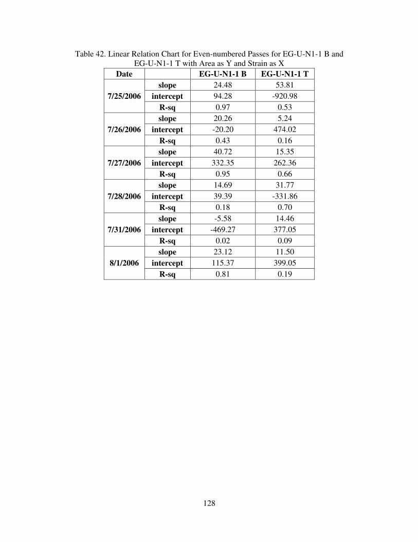
128
Table 42. Linear Relation Chart for Even-numbered Passes for EG-U-N1-1 B and
EG-U-N1-1 T with Area as Y and Strain as X
Date EG-U-N1-1 B EG-U-N1-1 T
7/25/2006
slope 24.48 53.81
intercept 94.28 -920.98
R-sq 0.97 0.53
7/26/2006
slope 20.26 5.24
intercept -20.20 474.02
R-sq 0.43 0.16
7/27/2006
slope 40.72 15.35
intercept 332.35 262.36
R-sq 0.95 0.66
7/28/2006
slope 14.69 31.77
intercept 39.39 -331.86
R-sq 0.18 0.70
7/31/2006
slope -5.58 14.46
intercept -469.27 377.05
R-sq 0.02 0.09
8/1/2006
slope 23.12 11.50
intercept 115.37 399.05
R-sq 0.81 0.19
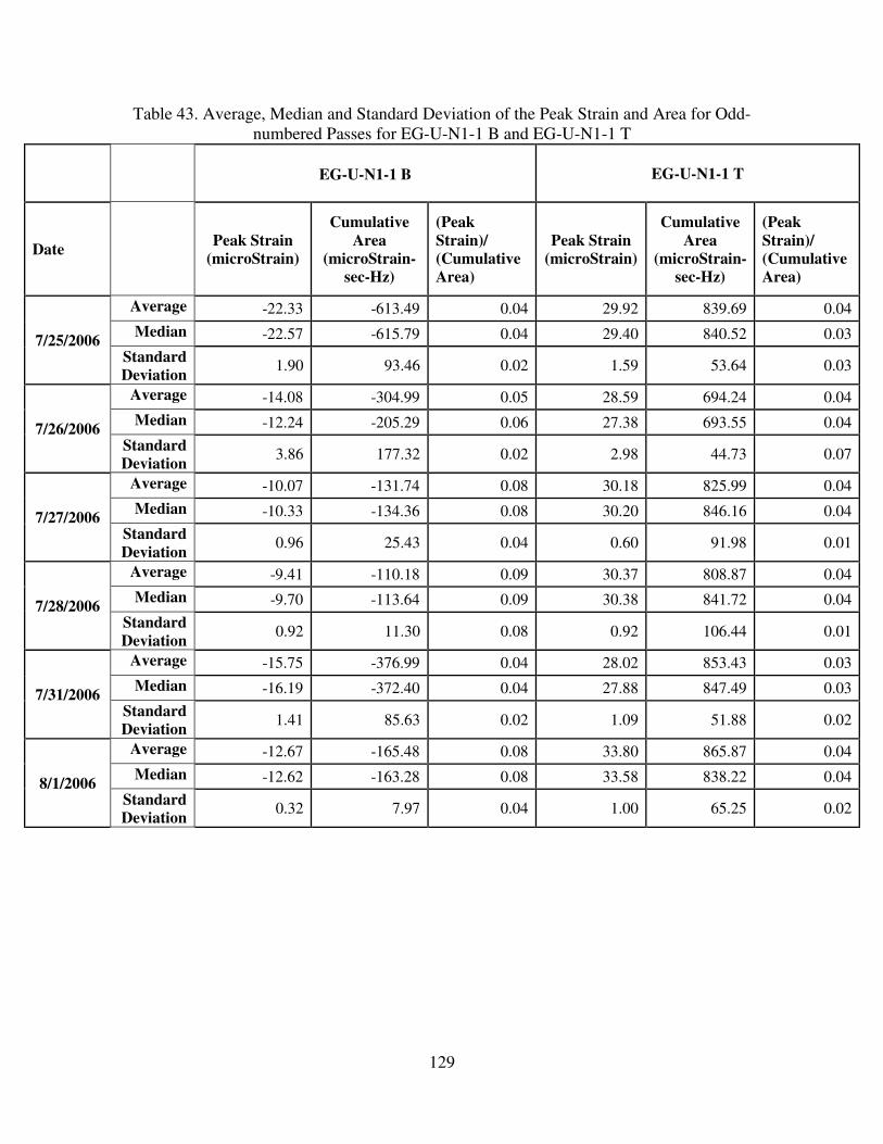
129
Table 43. Average, Median and Standard Deviation of the Peak Strain and Area for Odd-
numbered Passes for EG-U-N1-1 B and EG-U-N1-1 T
EG-U-N1-1 B
EG-U-N1-1 T
Date
Peak Strain (microStrain)
Cumulative
Area (microStrain-
sec-Hz)
(Peak
Strain)/
(Cumulative
Area)
Peak Strain (microStrain)
Cumulative
Area (microStrain-
sec-Hz)
(Peak
Strain)/
(Cumulative
Area)
7/25/2006
Average -22.33 -613.49 0.04 29.92 839.69 0.04
Median -22.57 -615.79 0.04 29.40 840.52 0.03
Standard
Deviation 1.90 93.46 0.02 1.59 53.64 0.03
7/26/2006
Average -14.08 -304.99 0.05 28.59 694.24 0.04
Median -12.24 -205.29 0.06 27.38 693.55 0.04
Standard
Deviation 3.86 177.32 0.02 2.98 44.73 0.07
7/27/2006
Average -10.07 -131.74 0.08 30.18 825.99 0.04
Median -10.33 -134.36 0.08 30.20 846.16 0.04
Standard
Deviation 0.96 25.43 0.04 0.60 91.98 0.01
7/28/2006
Average -9.41 -110.18 0.09 30.37 808.87 0.04
Median -9.70 -113.64 0.09 30.38 841.72 0.04
Standard
Deviation 0.92 11.30 0.08 0.92 106.44 0.01
7/31/2006
Average -15.75 -376.99 0.04 28.02 853.43 0.03
Median -16.19 -372.40 0.04 27.88 847.49 0.03
Standard
Deviation 1.41 85.63 0.02 1.09 51.88 0.02
8/1/2006
Average -12.67 -165.48 0.08 33.80 865.87 0.04
Median -12.62 -163.28 0.08 33.58 838.22 0.04
Standard
Deviation 0.32 7.97 0.04 1.00 65.25 0.02
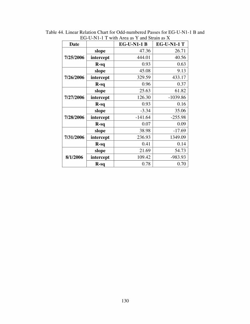
130
Table 44. Linear Relation Chart for Odd-numbered Passes for EG-U-N1-1 B and
EG-U-N1-1 T with Area as Y and Strain as X
Date EG-U-N1-1 B EG-U-N1-1 T
7/25/2006
slope 47.36 26.71
intercept 444.01 40.56
R-sq 0.93 0.63
7/26/2006
slope 45.08 9.13
intercept 329.59 433.17
R-sq 0.96 0.37
7/27/2006
slope 25.63 61.82
intercept 126.30 -1039.86
R-sq 0.93 0.16
7/28/2006
slope -3.34 35.06
intercept -141.64 -255.98
R-sq 0.07 0.09
7/31/2006
slope 38.98 -17.69
intercept 236.93 1349.09
R-sq 0.41 0.14
8/1/2006
slope 21.69 54.73
intercept 109.42 -983.93
R-sq 0.78 0.70
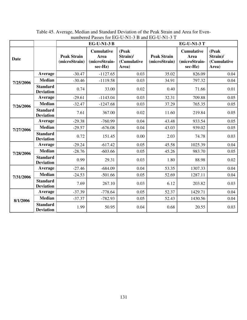
131
Table 45. Average, Median and Standard Deviation of the Peak Strain and Area for Even-
numbered Passes for EG-U-N1-3 B and EG-U-N1-3 T
EG-U-N1-3 B EG-U-N1-3 T
Date
Peak Strain (microStrain)
Cumulative
Area (microStrain-
sec-Hz)
(Peak
Strain)/
(Cumulative
Area)
Peak Strain (microStrain)
Cumulative
Area (microStrain-
sec-Hz)
(Peak
Strain)/
(Cumulative
Area)
7/25/2006
Average -30.47 -1127.65 0.03 35.02 826.09 0.04
Median -30.46 -1119.58 0.03 34.91 797.32 0.04
Standard
Deviation 0.74 33.00 0.02 0.40 71.66 0.01
7/26/2006
Average -29.61 -1143.04 0.03 32.31 709.88 0.05
Median -32.47 -1247.68 0.03 37.29 765.35 0.05
Standard
Deviation 7.61 367.00 0.02 11.60 219.84 0.05
7/27/2006
Average -29.38 -760.99 0.04 43.48 933.54 0.05
Median -29.57 -676.08 0.04 43.03 939.02 0.05
Standard
Deviation 0.72 151.45 0.00 2.03 74.78 0.03
7/28/2006
Average -29.24 -617.42 0.05 45.58 1025.39 0.04
Median -28.76 -603.66 0.05 45.26 983.70 0.05
Standard
Deviation 0.99 29.31 0.03 1.80 88.98 0.02
7/31/2006
Average -27.46 -684.09 0.04 53.35 1307.33 0.04
Median -24.53 -501.66 0.05 52.69 1287.11 0.04
Standard
Deviation 7.69 267.10 0.03 6.12 203.82 0.03
8/1/2006
Average -37.39 -778.64 0.05 52.37 1429.71 0.04
Median -37.37 -782.93 0.05 52.43 1430.56 0.04
Standard
Deviation 1.99 50.95 0.04 0.68 20.55 0.03
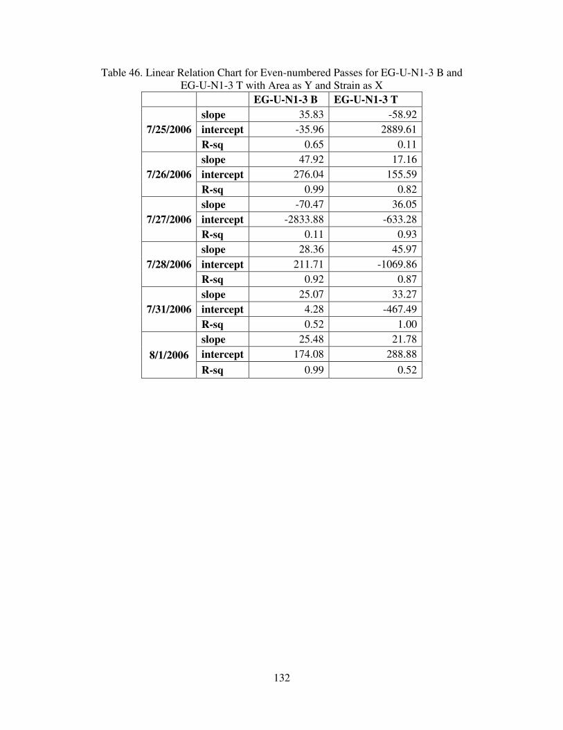
132
Table 46. Linear Relation Chart for Even-numbered Passes for EG-U-N1-3 B and
EG-U-N1-3 T with Area as Y and Strain as X
EG-U-N1-3 B EG-U-N1-3 T
7/25/2006
slope 35.83 -58.92
intercept -35.96 2889.61
R-sq 0.65 0.11
7/26/2006
slope 47.92 17.16
intercept 276.04 155.59
R-sq 0.99 0.82
7/27/2006
slope -70.47 36.05
intercept -2833.88 -633.28
R-sq 0.11 0.93
7/28/2006
slope 28.36 45.97
intercept 211.71 -1069.86
R-sq 0.92 0.87
7/31/2006
slope 25.07 33.27
intercept 4.28 -467.49
R-sq 0.52 1.00
8/1/2006
slope 25.48 21.78
intercept 174.08 288.88
R-sq 0.99 0.52

133
Table 47. Average, Median and Standard Deviation of the Peak Strain and Area for Odd-
numbered Passes for EG-U-N1-3 B and EG-U-N1-3T
EG-U-N1-3 B
EG-U-N1-3 T
Date
Peak Strain (microStrain)
Cumulative
Area (microStrain-
sec-Hz)
(Peak
Strain)/
(Cumulative
Area)
Peak Strain (microStrain)
Cumulative
Area (microStrain-
sec-Hz)
(Peak
Strain)/
(Cumulative
Area)
7/25/2006
Average -32.13 -1168.73 0.03 37.62 1140.50 0.03
Median -31.79 -1171.43 0.03 37.88 1129.74 0.03
Standard
Deviation 1.31 31.40 0.04 0.84 55.74 0.02
7/26/2006
Average -35.51 -1303.49 0.03 38.30 1047.16 0.04
Median -35.58 -1271.45 0.03 37.39 1081.34 0.03
Standard
Deviation 3.38 152.47 0.02 2.67 104.30 0.03
7/27/2006
Average -31.09 -934.26 0.03 39.11 1257.91 0.03
Median -31.18 -934.46 0.03 39.26 1258.34 0.03
Standard
Deviation 0.53 31.09 0.02 1.41 83.46 0.02
7/28/2006
Average -30.14 -819.95 0.04 39.74 1346.05 0.03
Median -29.81 -801.33 0.04 38.75 1306.70 0.03
Standard
Deviation 0.93 34.25 0.03 2.07 104.34 0.02
7/31/2006
Average -29.48 -793.22 0.04 32.70 997.05 0.03
Median -29.69 -867.29 0.03 18.97 670.41 0.03
Standard
Deviation 6.49 222.39 0.03 16.04 608.13 0.03
8/1/2006
Average -37.93 -896.71 0.04 46.89 1614.72 0.03
Median -38.20 -898.40 0.04 47.08 1629.98 0.03
Standard
Deviation 1.93 52.30 0.04 1.27 46.56 0.03
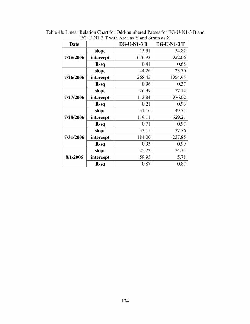
134
Table 48. Linear Relation Chart for Odd-numbered Passes for EG-U-N1-3 B and
EG-U-N1-3 T with Area as Y and Strain as X
Date EG-U-N1-3 B EG-U-N1-3 T
7/25/2006
slope 15.31 54.82
intercept -676.93 -922.06
R-sq 0.41 0.68
7/26/2006
slope 44.26 -23.70
intercept 268.45 1954.95
R-sq 0.96 0.37
7/27/2006
slope 26.39 57.12
intercept -113.84 -976.02
R-sq 0.21 0.93
7/28/2006
slope 31.16 49.71
intercept 119.11 -629.21
R-sq 0.71 0.97
7/31/2006
slope 33.15 37.76
intercept 184.00 -237.85
R-sq 0.93 0.99
8/1/2006
slope 25.22 34.31
intercept 59.95 5.78
R-sq 0.87 0.87
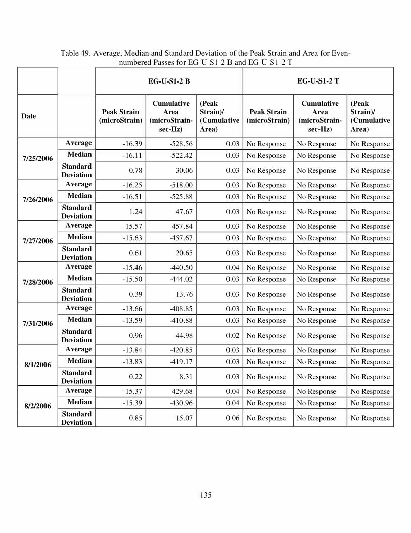
135
Table 49. Average, Median and Standard Deviation of the Peak Strain and Area for Even-
numbered Passes for EG-U-S1-2 B and EG-U-S1-2 T
EG-U-S1-2 B
EG-U-S1-2 T
Date
Peak Strain (microStrain)
Cumulative
Area (microStrain-
sec-Hz)
(Peak
Strain)/
(Cumulative
Area)
Peak Strain (microStrain)
Cumulative
Area (microStrain-
sec-Hz)
(Peak
Strain)/
(Cumulative
Area)
7/25/2006
Average -16.39 -528.56 0.03 No Response No Response No Response
Median -16.11 -522.42 0.03 No Response No Response No Response
Standard
Deviation 0.78 30.06 0.03 No Response No Response No Response
7/26/2006
Average -16.25 -518.00 0.03 No Response No Response No Response
Median -16.51 -525.88 0.03 No Response No Response No Response
Standard
Deviation 1.24 47.67 0.03 No Response No Response No Response
7/27/2006
Average -15.57 -457.84 0.03 No Response No Response No Response
Median -15.63 -457.67 0.03 No Response No Response No Response
Standard
Deviation 0.61 20.65 0.03 No Response No Response No Response
7/28/2006
Average -15.46 -440.50 0.04 No Response No Response No Response
Median -15.50 -444.02 0.03 No Response No Response No Response
Standard
Deviation 0.39 13.76 0.03 No Response No Response No Response
7/31/2006
Average -13.66 -408.85 0.03 No Response No Response No Response
Median -13.59 -410.88 0.03 No Response No Response No Response
Standard
Deviation 0.96 44.98 0.02 No Response No Response No Response
8/1/2006
Average -13.84 -420.85 0.03 No Response No Response No Response
Median -13.83 -419.17 0.03 No Response No Response No Response
Standard
Deviation 0.22 8.31 0.03 No Response No Response No Response
8/2/2006
Average -15.37 -429.68 0.04 No Response No Response No Response
Median -15.39 -430.96 0.04 No Response No Response No Response
Standard
Deviation 0.85 15.07 0.06 No Response No Response No Response
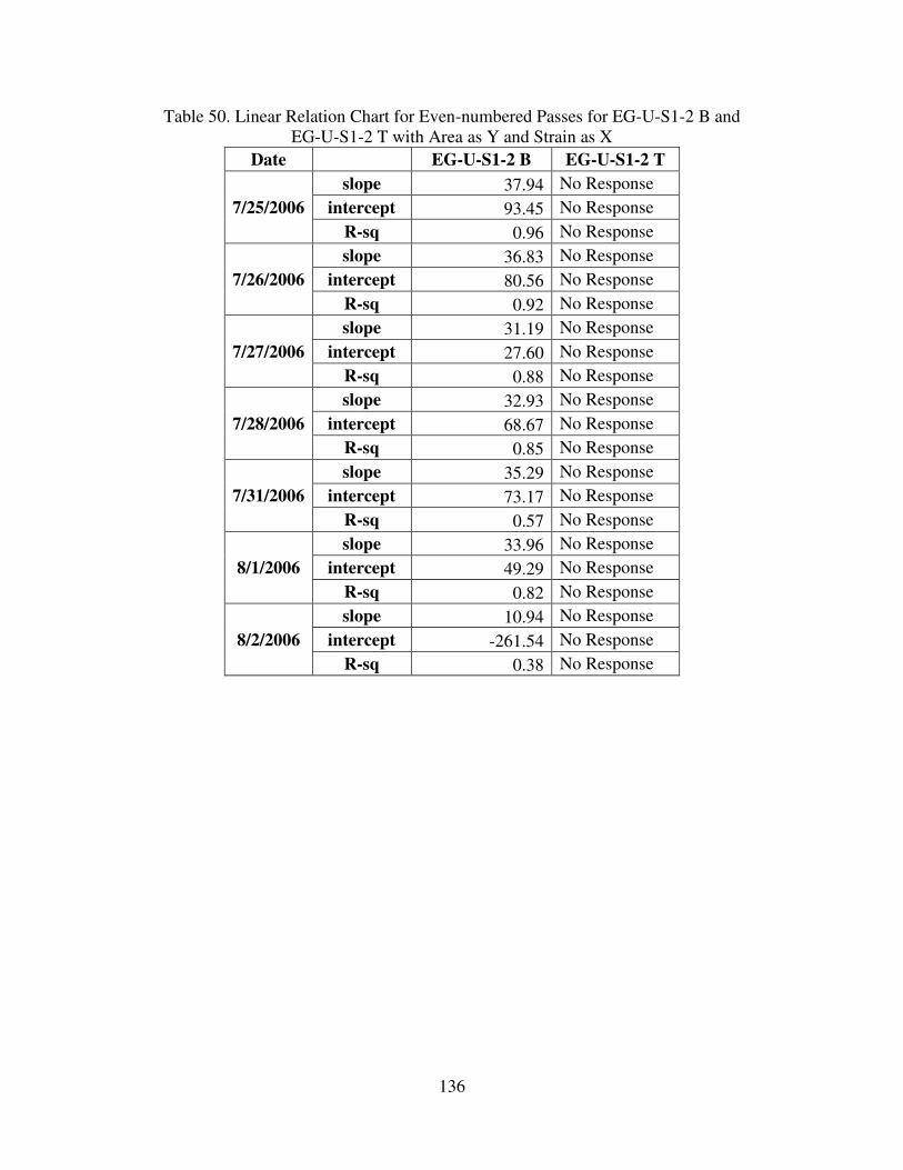
136
Table 50. Linear Relation Chart for Even-numbered Passes for EG-U-S1-2 B and
EG-U-S1-2 T with Area as Y and Strain as X
Date EG-U-S1-2 B EG-U-S1-2 T
7/25/2006
slope 37.94 No Response
intercept 93.45 No Response
R-sq 0.96 No Response
7/26/2006
slope 36.83 No Response
intercept 80.56 No Response
R-sq 0.92 No Response
7/27/2006
slope 31.19 No Response
intercept 27.60 No Response
R-sq 0.88 No Response
7/28/2006
slope 32.93 No Response
intercept 68.67 No Response
R-sq 0.85 No Response
7/31/2006
slope 35.29 No Response
intercept 73.17 No Response
R-sq 0.57 No Response
8/1/2006
slope 33.96 No Response
intercept 49.29 No Response
R-sq 0.82 No Response
8/2/2006
slope 10.94 No Response
intercept -261.54 No Response
R-sq 0.38 No Response
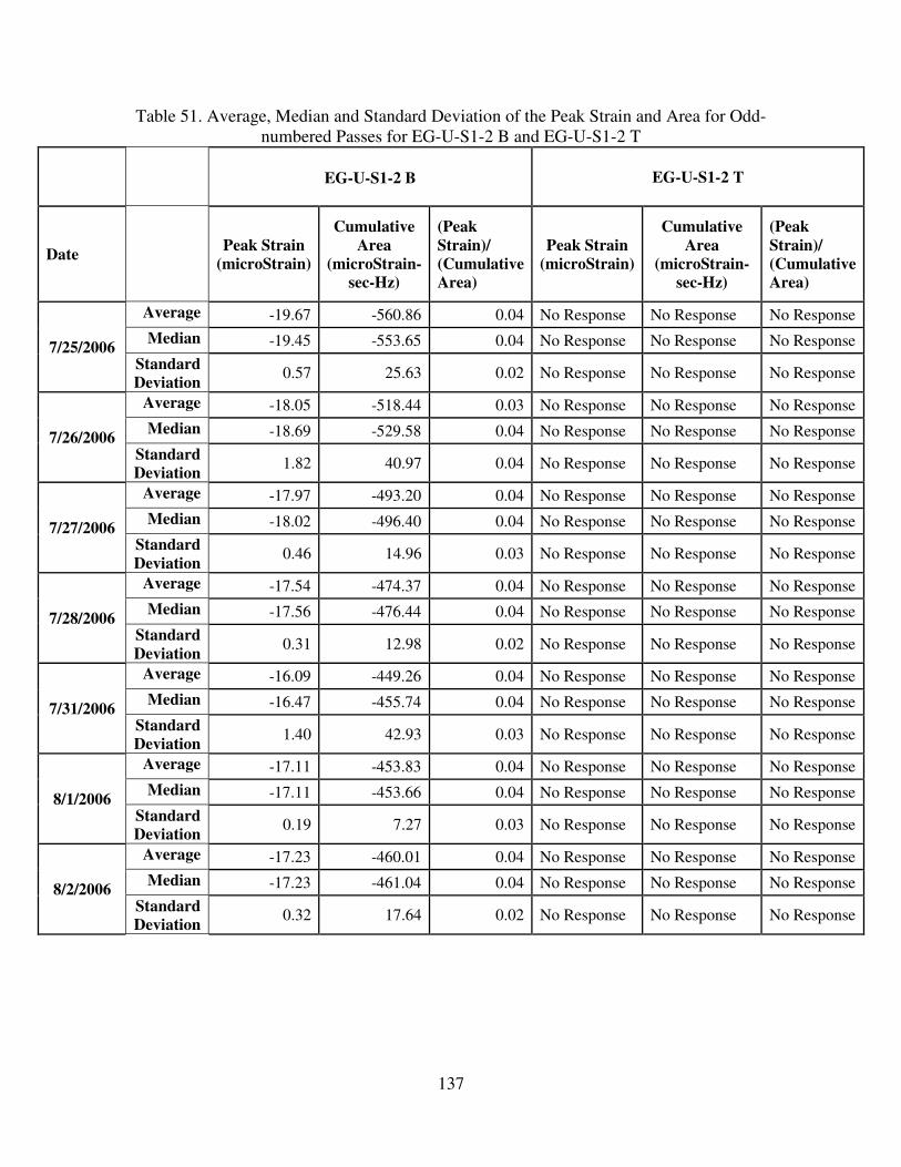
137
Table 51. Average, Median and Standard Deviation of the Peak Strain and Area for Odd-
numbered Passes for EG-U-S1-2 B and EG-U-S1-2 T
EG-U-S1-2 B
EG-U-S1-2 T
Date
Peak Strain (microStrain)
Cumulative
Area (microStrain-
sec-Hz)
(Peak
Strain)/
(Cumulative
Area)
Peak Strain (microStrain)
Cumulative
Area (microStrain-
sec-Hz)
(Peak
Strain)/
(Cumulative
Area)
7/25/2006
Average -19.67 -560.86 0.04 No Response No Response No Response
Median -19.45 -553.65 0.04 No Response No Response No Response
Standard
Deviation 0.57 25.63 0.02 No Response No Response No Response
7/26/2006
Average -18.05 -518.44 0.03 No Response No Response No Response
Median -18.69 -529.58 0.04 No Response No Response No Response
Standard
Deviation 1.82 40.97 0.04 No Response No Response No Response
7/27/2006
Average -17.97 -493.20 0.04 No Response No Response No Response
Median -18.02 -496.40 0.04 No Response No Response No Response
Standard
Deviation 0.46 14.96 0.03 No Response No Response No Response
7/28/2006
Average -17.54 -474.37 0.04 No Response No Response No Response
Median -17.56 -476.44 0.04 No Response No Response No Response
Standard
Deviation 0.31 12.98 0.02 No Response No Response No Response
7/31/2006
Average -16.09 -449.26 0.04 No Response No Response No Response
Median -16.47 -455.74 0.04 No Response No Response No Response
Standard
Deviation 1.40 42.93 0.03 No Response No Response No Response
8/1/2006
Average -17.11 -453.83 0.04 No Response No Response No Response
Median -17.11 -453.66 0.04 No Response No Response No Response
Standard
Deviation 0.19 7.27 0.03 No Response No Response No Response
8/2/2006
Average -17.23 -460.01 0.04 No Response No Response No Response
Median -17.23 -461.04 0.04 No Response No Response No Response
Standard
Deviation 0.32 17.64 0.02 No Response No Response No Response

138
Table 52. Linear Relation Chart for Odd-numbered Passes for EG-U-S1-2 B and
EG-U-S1-2 T with Area as Y and Strain as X
Date EG-U-S1-2 B EG-U-S1-2 T
7/25/2006
slope 43.80 No Response
intercept 300.87 No Response
R-sq 0.93 No Response
7/26/2006
slope 22.10 No Response
intercept -119.46 No Response
R-sq 0.96 No Response
7/27/2006
slope 29.52 No Response
intercept 37.33 No Response
R-sq 0.84 No Response
7/28/2006
slope 31.10 No Response
intercept 71.21 No Response
R-sq 0.55 No Response
7/31/2006
slope 22.74 No Response
intercept -83.50 No Response
R-sq 0.55 No Response
8/1/2006
slope 23.82 No Response
intercept -46.39 No Response
R-sq 0.38 No Response
8/2/2006
slope 48.91 No Response
intercept 382.48 No Response
R-sq 0.79 No Response

139
Table 53. Average, Median and Standard Deviation of the Peak Strain and Area for Even-
numbered Passes for EG-U-S1-3 B and EG-U-S1-3 T
EG-U-S1-3 B
EG-U-S1-3 T
Date
Peak Strain (microStrain)
Cumulative
Area (microStrain-
sec-Hz)
(Peak
Strain)/
(Cumulative
Area)
Peak Strain (microStrain)
Cumulative
Area (microStrain-
sec-Hz)
(Peak
Strain)/
(Cumulative
Area)
7/25/2006
Average -55.86 -1652.33 0.03 54.24 1374.42 0.04
Median -56.11 -1653.57 0.03 54.39 1384.89 0.04
Standard
Deviation 0.93 25.85 0.04 1.09 36.30 0.03
7/26/2006
Average -49.37 -1456.62 0.03 53.27 1346.00 0.04
Median -51.54 -1507.85 0.03 54.41 1348.94 0.04
Standard
Deviation 6.68 187.99 0.04 8.13 182.77 0.04
7/27/2006
Average -44.06 -1270.63 0.03 52.06 1260.38 0.04
Median -43.91 -1272.54 0.03 51.53 1240.17 0.04
Standard
Deviation 0.54 18.27 0.03 1.57 52.10 0.03
7/28/2006
Average -42.33 -1211.08 0.03 51.36 1213.33 0.04
Median -41.65 -1191.19 0.03 50.52 1181.37 0.04
Standard
Deviation 1.37 39.19 0.03 2.08 68.03 0.03
7/31/2006
Average -38.23 -1165.72 0.03 49.41 1264.38 0.04
Median -40.21 -1229.12 0.03 50.65 1339.39 0.04
Standard
Deviation 6.10 162.16 0.04 11.44 302.63 0.04
8/1/2006
Average -39.29 -1166.31 0.03 44.45 1217.00 0.04
Median -39.25 -1165.51 0.03 44.49 1215.46 0.04
Standard
Deviation 0.28 9.85 0.03 0.49 16.52 0.03
8/2/2006
Average -43.56 -1251.35 0.03 56.27 1356.64 0.04
Median -43.62 -1252.14 0.03 56.50 1364.13 0.04
Standard
Deviation 0.84 12.68 0.07 1.21 27.92 0.04
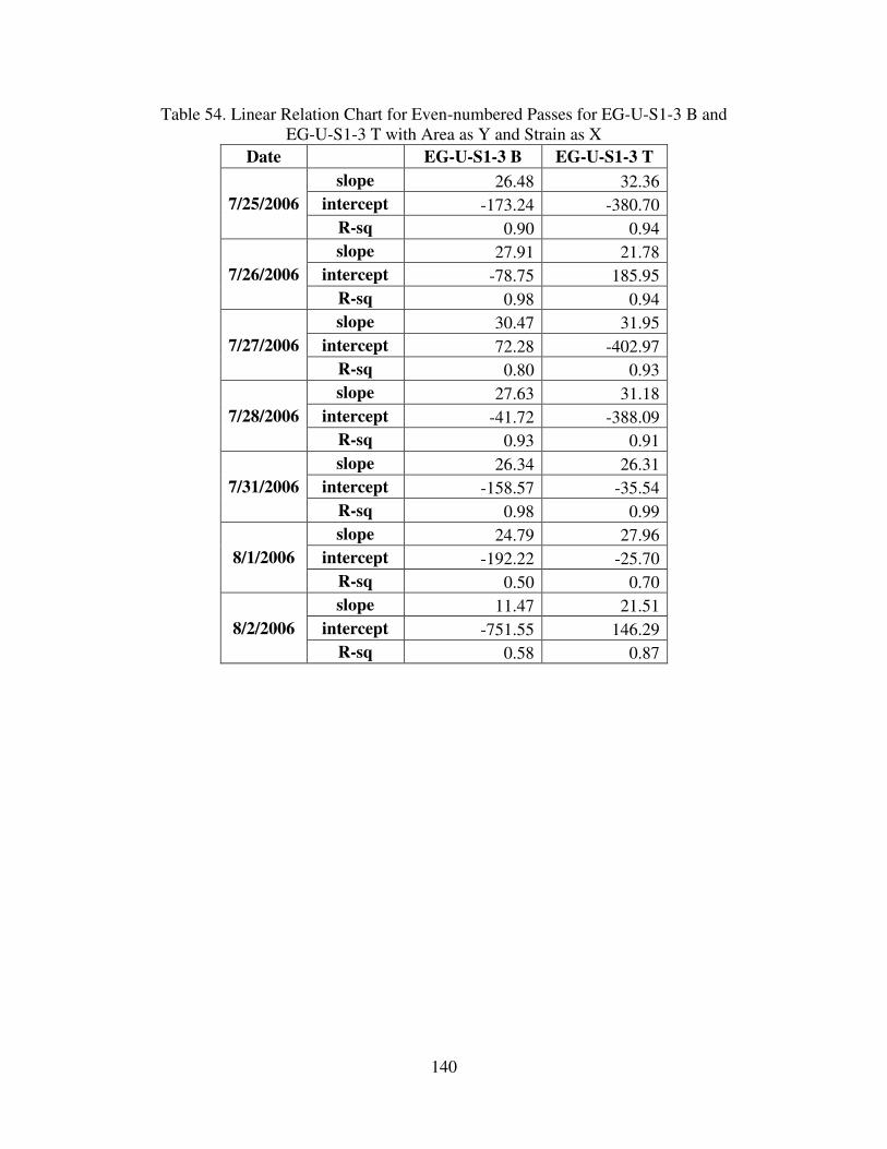
140
Table 54. Linear Relation Chart for Even-numbered Passes for EG-U-S1-3 B and
EG-U-S1-3 T with Area as Y and Strain as X
Date EG-U-S1-3 B EG-U-S1-3 T
7/25/2006
slope 26.48 32.36
intercept -173.24 -380.70
R-sq 0.90 0.94
7/26/2006
slope 27.91 21.78
intercept -78.75 185.95
R-sq 0.98 0.94
7/27/2006
slope 30.47 31.95
intercept 72.28 -402.97
R-sq 0.80 0.93
7/28/2006
slope 27.63 31.18
intercept -41.72 -388.09
R-sq 0.93 0.91
7/31/2006
slope 26.34 26.31
intercept -158.57 -35.54
R-sq 0.98 0.99
8/1/2006
slope 24.79 27.96
intercept -192.22 -25.70
R-sq 0.50 0.70
8/2/2006
slope 11.47 21.51
intercept -751.55 146.29
R-sq 0.58 0.87
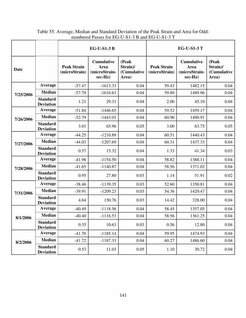
141
Table 55. Average, Median and Standard Deviation of the Peak Strain and Area for Odd-
numbered Passes for EG-U-S1-3 B and EG-U-S1-3 T
EG-U-S1-3 B
EG-U-S1-3 T
Date
Peak Strain (microStrain)
Cumulative
Area (microStrain-
sec-Hz)
(Peak
Strain)/
(Cumulative
Area)
Peak Strain (microStrain)
Cumulative
Area (microStrain-
sec-Hz)
(Peak
Strain)/
(Cumulative
Area)
7/25/2006
Average -57.47 -1613.33 0.04 59.43 1482.15 0.04
Median -57.79 -1610.63 0.04 59.89 1489.96 0.04
Standard
Deviation 1.21 29.31 0.04 2.00 45.10 0.04
7/26/2006
Average -51.84 -1446.65 0.04 59.52 1459.17 0.04
Median -52.79 -1443.03 0.04 60.90 1490.91 0.04
Standard
Deviation 3.01 65.96 0.05 3.00 63.75 0.05
7/27/2006
Average -44.25 -1210.89 0.04 60.51 1440.43 0.04
Median -44.03 -1207.69 0.04 60.31 1437.33 0.04
Standard
Deviation 0.57 15.32 0.04 1.33 41.34 0.03
7/28/2006
Average -41.98 -1154.50 0.04 58.82 1388.11 0.04
Median -41.65 -1140.87 0.04 58.56 1371.02 0.04
Standard
Deviation 0.95 27.80 0.03 1.14 51.91 0.02
7/31/2006
Average -38.46 -1139.35 0.03 52.60 1350.81 0.04
Median -39.91 -1209.23 0.03 54.36 1420.47 0.04
Standard
Deviation 4.64 150.76 0.03 14.42 328.00 0.04
8/1/2006
Average -40.49 -1118.56 0.04 58.45 1357.05 0.04
Median -40.40 -1116.53 0.04 58.56 1361.25 0.04
Standard
Deviation 0.35 10.63 0.03 0.56 12.80 0.04
8/2/2006
Average -41.70 -1185.14 0.04 59.95 1474.93 0.04
Median -41.72 -1187.33 0.04 60.27 1486.60 0.04
Standard
Deviation 0.53 11.03 0.05 1.10 30.72 0.04
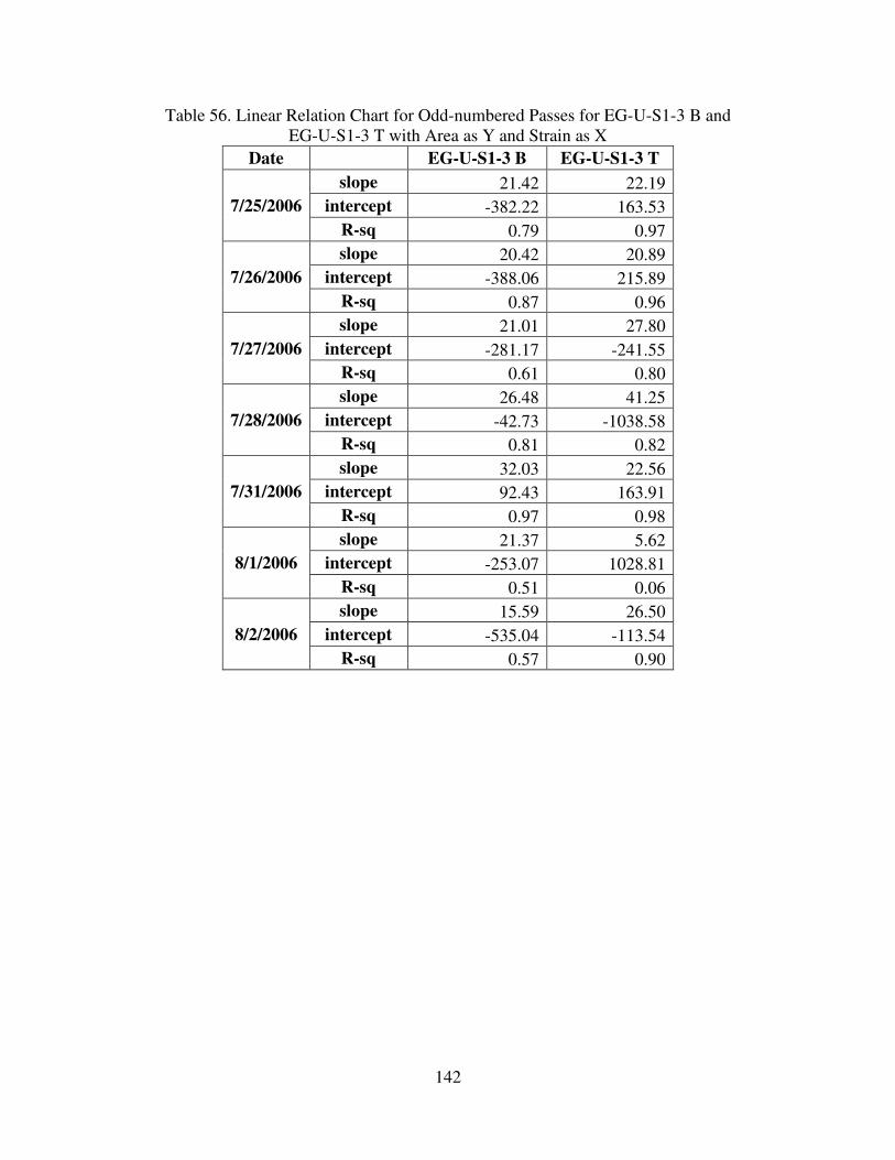
142
Table 56. Linear Relation Chart for Odd-numbered Passes for EG-U-S1-3 B and
EG-U-S1-3 T with Area as Y and Strain as X
Date EG-U-S1-3 B EG-U-S1-3 T
7/25/2006
slope 21.42 22.19
intercept -382.22 163.53
R-sq 0.79 0.97
7/26/2006
slope 20.42 20.89
intercept -388.06 215.89
R-sq 0.87 0.96
7/27/2006
slope 21.01 27.80
intercept -281.17 -241.55
R-sq 0.61 0.80
7/28/2006
slope 26.48 41.25
intercept -42.73 -1038.58
R-sq 0.81 0.82
7/31/2006
slope 32.03 22.56
intercept 92.43 163.91
R-sq 0.97 0.98
8/1/2006
slope 21.37 5.62
intercept -253.07 1028.81
R-sq 0.51 0.06
8/2/2006
slope 15.59 26.50
intercept -535.04 -113.54
R-sq 0.57 0.90
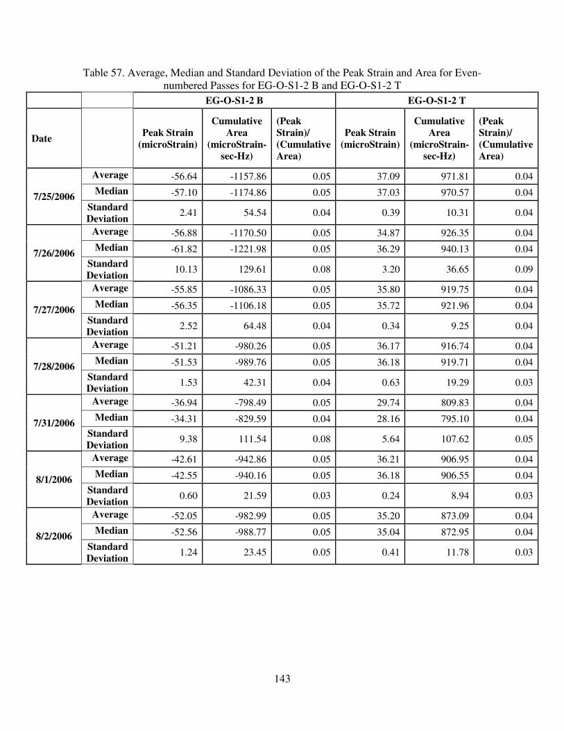
143
Table 57. Average, Median and Standard Deviation of the Peak Strain and Area for Even-
numbered Passes for EG-O-S1-2 B and EG-O-S1-2 T
EG-O-S1-2 B EG-O-S1-2 T
Date
Peak Strain (microStrain)
Cumulative
Area (microStrain-
sec-Hz)
(Peak
Strain)/
(Cumulative
Area)
Peak Strain (microStrain)
Cumulative
Area (microStrain-
sec-Hz)
(Peak
Strain)/
(Cumulative
Area)
7/25/2006
Average -56.64 -1157.86 0.05 37.09 971.81 0.04
Median -57.10 -1174.86 0.05 37.03 970.57 0.04
Standard
Deviation 2.41 54.54 0.04 0.39 10.31 0.04
7/26/2006
Average -56.88 -1170.50 0.05 34.87 926.35 0.04
Median -61.82 -1221.98 0.05 36.29 940.13 0.04
Standard
Deviation 10.13 129.61 0.08 3.20 36.65 0.09
7/27/2006
Average -55.85 -1086.33 0.05 35.80 919.75 0.04
Median -56.35 -1106.18 0.05 35.72 921.96 0.04
Standard
Deviation 2.52 64.48 0.04 0.34 9.25 0.04
7/28/2006
Average -51.21 -980.26 0.05 36.17 916.74 0.04
Median -51.53 -989.76 0.05 36.18 919.71 0.04
Standard
Deviation 1.53 42.31 0.04 0.63 19.29 0.03
7/31/2006
Average -36.94 -798.49 0.05 29.74 809.83 0.04
Median -34.31 -829.59 0.04 28.16 795.10 0.04
Standard
Deviation 9.38 111.54 0.08 5.64 107.62 0.05
8/1/2006
Average -42.61 -942.86 0.05 36.21 906.95 0.04
Median -42.55 -940.16 0.05 36.18 906.55 0.04
Standard
Deviation 0.60 21.59 0.03 0.24 8.94 0.03
8/2/2006
Average -52.05 -982.99 0.05 35.20 873.09 0.04
Median -52.56 -988.77 0.05 35.04 872.95 0.04
Standard
Deviation 1.24 23.45 0.05 0.41 11.78 0.03
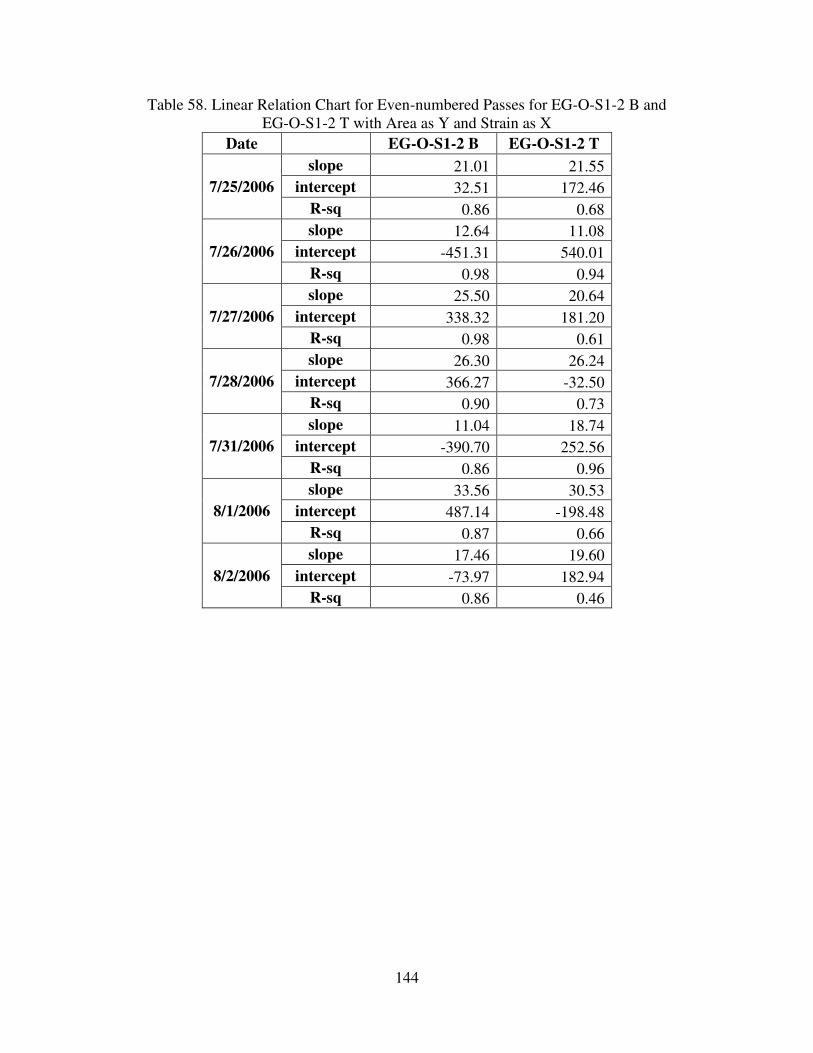
144
Table 58. Linear Relation Chart for Even-numbered Passes for EG-O-S1-2 B and
EG-O-S1-2 T with Area as Y and Strain as X
Date EG-O-S1-2 B EG-O-S1-2 T
7/25/2006
slope 21.01 21.55
intercept 32.51 172.46
R-sq 0.86 0.68
7/26/2006
slope 12.64 11.08
intercept -451.31 540.01
R-sq 0.98 0.94
7/27/2006
slope 25.50 20.64
intercept 338.32 181.20
R-sq 0.98 0.61
7/28/2006
slope 26.30 26.24
intercept 366.27 -32.50
R-sq 0.90 0.73
7/31/2006
slope 11.04 18.74
intercept -390.70 252.56
R-sq 0.86 0.96
8/1/2006
slope 33.56 30.53
intercept 487.14 -198.48
R-sq 0.87 0.66
8/2/2006
slope 17.46 19.60
intercept -73.97 182.94
R-sq 0.86 0.46

145
Table 59. Average, Median and Standard Deviation of the Peak Strain and Area for Odd-
numbered Passes for EG-O-S1-2 B and EG-O-S1-2 T
EG-O-S1-2 B EG-O-S1-2 T
Date
Peak Strain (microStrain)
Cumulative
Area (microStrain-
sec-Hz)
(Peak
Strain)/
(Cumulative
Area)
Peak Strain (microStrain)
Cumulative
Area (microStrain-
sec-Hz)
(Peak
Strain)/
(Cumulative
Area)
7/25/2006
Average -57.19 -1169.53 0.05 39.66 1026.44 0.04
Median -57.78 -1179.49 0.05 39.75 1028.20 0.04
Standard
Deviation 2.12 39.70 0.05 0.23 5.85 0.04
7/26/2006
Average -61.65 -1216.09 0.05 38.01 985.67 0.04
Median -62.09 -1222.13 0.05 38.56 1000.11 0.04
Standard
Deviation 1.24 31.22 0.04 1.05 30.07 0.03
7/27/2006
Average -51.07 -1006.49 0.05 37.64 972.33 0.04
Median -51.65 -1030.00 0.05 37.70 973.75 0.04
Standard
Deviation 3.65 78.01 0.05 0.36 9.66 0.04
7/28/2006
Average -44.12 -874.97 0.05 37.88 972.21 0.04
Median -44.60 -862.50 0.05 38.01 972.57 0.04
Standard
Deviation 1.93 49.44 0.04 0.56 14.12 0.04
7/31/2006
Average -29.79 -681.95 0.04 29.22 794.67 0.04
Median -30.72 -676.13 0.05 27.27 799.84 0.03
Standard
Deviation 3.18 93.74 0.03 6.04 145.57 0.04
8/1/2006
Average -41.04 -791.79 0.05 38.60 967.89 0.04
Median -40.91 -785.39 0.05 38.62 971.14 0.04
Standard
Deviation 0.89 26.25 0.03 0.46 10.31 0.04
8/2/2006
Average -42.39 -876.18 0.05 37.27 925.01 0.04
Median -42.70 -887.57 0.05 37.22 924.11 0.04
Standard
Deviation 0.73 25.33 0.03 0.28 8.14 0.03
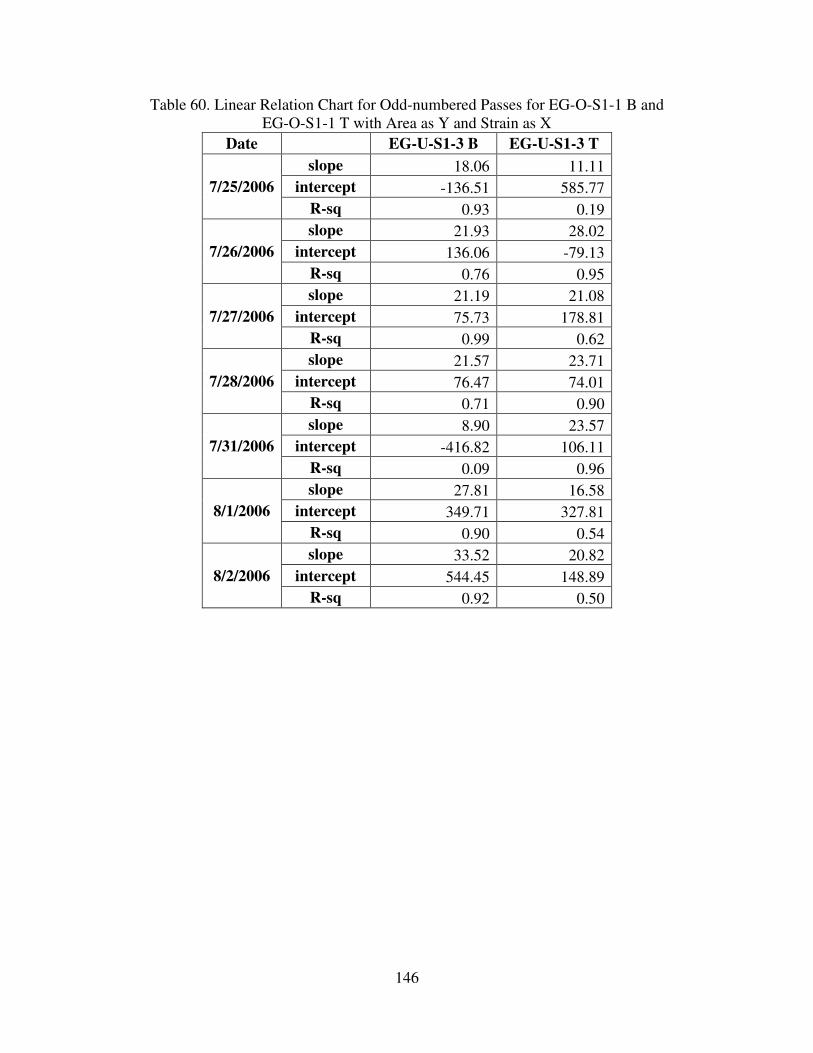
146
Table 60. Linear Relation Chart for Odd-numbered Passes for EG-O-S1-1 B and
EG-O-S1-1 T with Area as Y and Strain as X
Date EG-U-S1-3 B EG-U-S1-3 T
7/25/2006
slope 18.06 11.11
intercept -136.51 585.77
R-sq 0.93 0.19
7/26/2006
slope 21.93 28.02
intercept 136.06 -79.13
R-sq 0.76 0.95
7/27/2006
slope 21.19 21.08
intercept 75.73 178.81
R-sq 0.99 0.62
7/28/2006
slope 21.57 23.71
intercept 76.47 74.01
R-sq 0.71 0.90
7/31/2006
slope 8.90 23.57
intercept -416.82 106.11
R-sq 0.09 0.96
8/1/2006
slope 27.81 16.58
intercept 349.71 327.81
R-sq 0.90 0.54
8/2/2006
slope 33.52 20.82
intercept 544.45 148.89
R-sq 0.92 0.50
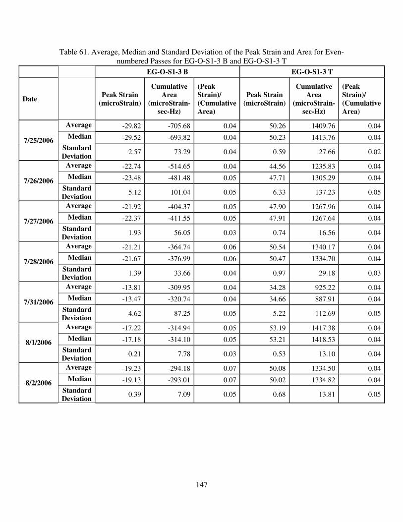
147
Table 61. Average, Median and Standard Deviation of the Peak Strain and Area for Even-
numbered Passes for EG-O-S1-3 B and EG-O-S1-3 T
EG-O-S1-3 B EG-O-S1-3 T
Date
Peak Strain (microStrain)
Cumulative
Area (microStrain-
sec-Hz)
(Peak
Strain)/
(Cumulative
Area)
Peak Strain (microStrain)
Cumulative
Area (microStrain-
sec-Hz)
(Peak
Strain)/
(Cumulative
Area)
7/25/2006
Average -29.82 -705.68 0.04 50.26 1409.76 0.04
Median -29.52 -693.82 0.04 50.23 1413.76 0.04
Standard
Deviation 2.57 73.29 0.04 0.59 27.66 0.02
7/26/2006
Average -22.74 -514.65 0.04 44.56 1235.83 0.04
Median -23.48 -481.48 0.05 47.71 1305.29 0.04
Standard
Deviation 5.12 101.04 0.05 6.33 137.23 0.05
7/27/2006
Average -21.92 -404.37 0.05 47.90 1267.96 0.04
Median -22.37 -411.55 0.05 47.91 1267.64 0.04
Standard
Deviation 1.93 56.05 0.03 0.74 16.56 0.04
7/28/2006
Average -21.21 -364.74 0.06 50.54 1340.17 0.04
Median -21.67 -376.99 0.06 50.47 1334.70 0.04
Standard
Deviation 1.39 33.66 0.04 0.97 29.18 0.03
7/31/2006
Average -13.81 -309.95 0.04 34.28 925.22 0.04
Median -13.47 -320.74 0.04 34.66 887.91 0.04
Standard
Deviation 4.62 87.25 0.05 5.22 112.69 0.05
8/1/2006
Average -17.22 -314.94 0.05 53.19 1417.38 0.04
Median -17.18 -314.10 0.05 53.21 1418.53 0.04
Standard
Deviation 0.21 7.78 0.03 0.53 13.10 0.04
8/2/2006
Average -19.23 -294.18 0.07 50.08 1334.50 0.04
Median -19.13 -293.01 0.07 50.02 1334.82 0.04
Standard
Deviation 0.39 7.09 0.05 0.68 13.81 0.05
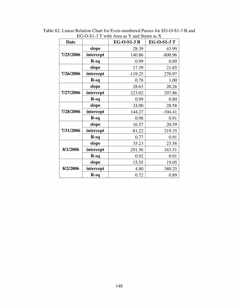
148
Table 62. Linear Relation Chart for Even-numbered Passes for EG-O-S1-3 B and
EG-O-S1-3 T with Area as Y and Strain as X
Date EG-O-S1-3 B EG-O-S1-3 T
7/25/2006
slope 28.39 43.99
intercept 140.86 -800.96
R-sq 0.99 0.89
7/26/2006
slope 17.39 21.65
intercept -119.25 270.97
R-sq 0.78 1.00
7/27/2006
slope 28.63 20.26
intercept 223.02 297.86
R-sq 0.99 0.80
7/28/2006
slope 24.00 28.58
intercept 144.27 -104.41
R-sq 0.98 0.91
7/31/2006
slope 16.57 20.59
intercept -81.22 219.35
R-sq 0.77 0.91
8/1/2006
slope 35.23 23.58
intercept 291.56 163.51
R-sq 0.92 0.91
8/2/2006
slope 15.55 19.05
intercept 4.80 380.25
R-sq 0.72 0.89
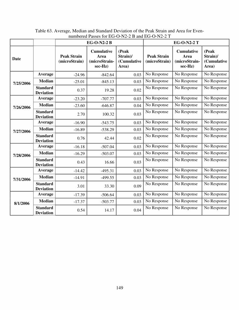
149
Table 63. Average, Median and Standard Deviation of the Peak Strain and Area for Even-
numbered Passes for EG-O-N2-2 B and EG-O-N2-2 T
EG-O-N2-2 B EG-O-N2-2 T
Date
Peak Strain (microStrain)
Cumulative
Area (microStrain-
sec-Hz)
(Peak
Strain)/
(Cumulative
Area)
Peak Strain (microStrain)
Cumulative
Area (microStrain-
sec-Hz)
(Peak
Strain)/
(Cumulative
Area)
7/25/2006
Average -24.96 -842.64 0.03 No Response No Response No Response
Median -25.01 -845.13 0.03 No Response No Response No Response
Standard
Deviation 0.37 19.28 0.02
No Response No Response No Response
7/26/2006
Average -23.20 -707.77 0.03 No Response No Response No Response
Median -23.60 -646.87 0.04 No Response No Response No Response
Standard
Deviation 2.70 100.32 0.03
No Response No Response No Response
7/27/2006
Average -16.90 -543.75 0.03 No Response No Response No Response
Median -16.89 -538.29 0.03 No Response No Response No Response
Standard
Deviation 0.76 42.44 0.02
No Response No Response No Response
7/28/2006
Average -16.18 -507.04 0.03 No Response No Response No Response
Median -16.29 -503.07 0.03 No Response No Response No Response
Standard
Deviation 0.43 16.66 0.03
No Response No Response No Response
7/31/2006
Average -14.42 -495.31 0.03 No Response No Response No Response
Median -14.91 -499.55 0.03 No Response No Response No Response
Standard
Deviation 3.01 33.30 0.09
No Response No Response No Response
8/1/2006
Average -17.39 -506.64 0.03 No Response No Response No Response
Median -17.37 -503.77 0.03 No Response No Response No Response
Standard
Deviation 0.54 14.17 0.04
No Response No Response No Response
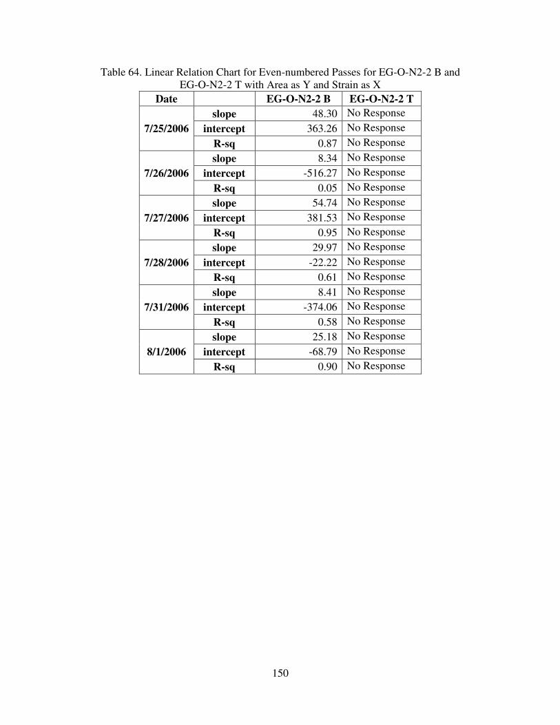
150
Table 64. Linear Relation Chart for Even-numbered Passes for EG-O-N2-2 B and
EG-O-N2-2 T with Area as Y and Strain as X
Date EG-O-N2-2 B EG-O-N2-2 T
7/25/2006
slope 48.30 No Response
intercept 363.26 No Response
R-sq 0.87 No Response
7/26/2006
slope 8.34 No Response
intercept -516.27 No Response
R-sq 0.05 No Response
7/27/2006
slope 54.74 No Response
intercept 381.53 No Response
R-sq 0.95 No Response
7/28/2006
slope 29.97 No Response
intercept -22.22 No Response
R-sq 0.61 No Response
7/31/2006
slope 8.41 No Response
intercept -374.06 No Response
R-sq 0.58 No Response
8/1/2006
slope 25.18 No Response
intercept -68.79 No Response
R-sq 0.90 No Response

151
Table 65. Average, Median and Standard Deviation of the Peak Strain and Area for Odd-
numbered Passes for EG-O-N2-2 B and EG-O-N2-2 T
EG-O-N2-2 B EG-O-N2-2 T
Date
Peak Strain (microStrain)
Cumulative
Area (microStrain-
sec-Hz)
(Peak
Strain)/
(Cumulative
Area)
Peak Strain (microStrain)
Cumulative
Area (microStrain-
sec-Hz)
(Peak
Strain)/
(Cumulative
Area)
7/25/2006
Average -26.23 -662.40 0.04 No Response No Response No Response
Median -26.21 -661.98 0.04 No Response No Response No Response
Standard
Deviation 0.31 7.50 0.04
No Response No Response No Response
7/26/2006
Average -23.71 -629.73 0.04 No Response No Response No Response
Median -24.84 -617.49 0.04 No Response No Response No Response
Standard
Deviation 2.44 33.86 0.07
No Response No Response No Response
7/27/2006
Average -15.32 -413.27 0.04 No Response No Response No Response
Median -15.01 -407.11 0.04 No Response No Response No Response
Standard
Deviation 1.25 28.65 0.04
No Response No Response No Response
7/28/2006
Average -13.29 -367.42 0.04 No Response No Response No Response
Median -13.24 -371.04 0.04 No Response No Response No Response
Standard
Deviation 0.46 13.65 0.03
No Response No Response No Response
7/31/2006
Average -10.68 -270.47 0.04 No Response No Response No Response
Median -10.48 -252.56 0.04 No Response No Response No Response
Standard
Deviation 5.09 128.10 0.04
No Response No Response No Response
8/1/2006
Average -12.53 -347.39 0.04 No Response No Response No Response
Median -12.48 -347.01 0.04 No Response No Response No Response
Standard
Deviation 0.40 14.59 0.03
No Response No Response No Response
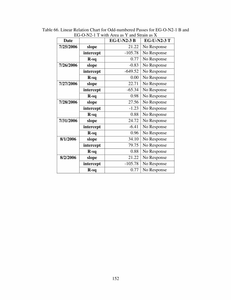
152
Table 66. Linear Relation Chart for Odd-numbered Passes for EG-O-N2-1 B and
EG-O-N2-1 T with Area as Y and Strain as X
Date EG-U-N2-3 B EG-U-N2-3 T
7/25/2006 slope 21.22 No Response
intercept -105.78 No Response
R-sq 0.77 No Response
7/26/2006 slope -0.83 No Response
intercept -649.52 No Response
R-sq 0.00 No Response
7/27/2006 slope 22.71 No Response
intercept -65.34 No Response
R-sq 0.98 No Response
7/28/2006 slope 27.56 No Response
intercept -1.23 No Response
R-sq 0.88 No Response
7/31/2006 slope 24.72 No Response
intercept -6.41 No Response
R-sq 0.96 No Response
8/1/2006 slope 34.10 No Response
intercept 79.75 No Response
R-sq 0.88 No Response
8/2/2006 slope 21.22 No Response
intercept -105.78 No Response
R-sq 0.77 No Response
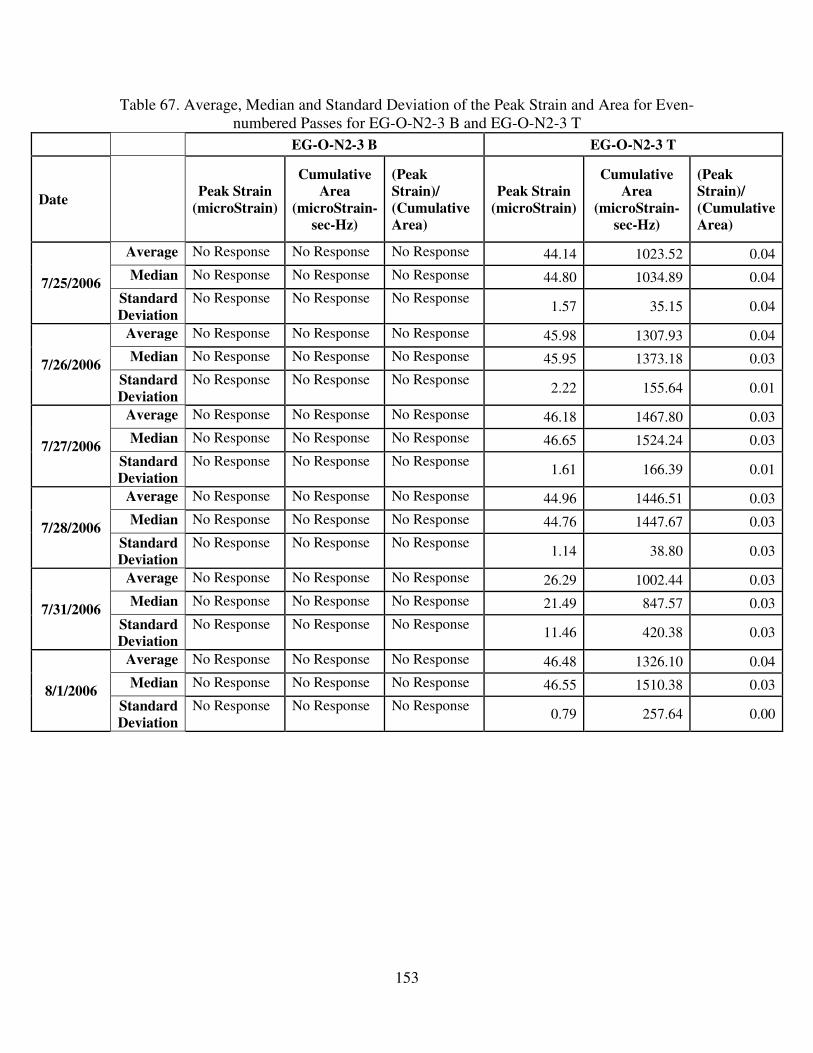
153
Table 67. Average, Median and Standard Deviation of the Peak Strain and Area for Even-
numbered Passes for EG-O-N2-3 B and EG-O-N2-3 T
EG-O-N2-3 B EG-O-N2-3 T
Date
Peak Strain (microStrain)
Cumulative
Area (microStrain-
sec-Hz)
(Peak
Strain)/
(Cumulative
Area)
Peak Strain (microStrain)
Cumulative
Area (microStrain-
sec-Hz)
(Peak
Strain)/
(Cumulative
Area)
7/25/2006
Average No Response No Response No Response 44.14 1023.52 0.04
Median No Response No Response No Response 44.80 1034.89 0.04
Standard
Deviation No Response No Response No Response
1.57 35.15 0.04
7/26/2006
Average No Response No Response No Response 45.98 1307.93 0.04
Median No Response No Response No Response 45.95 1373.18 0.03
Standard
Deviation No Response No Response No Response
2.22 155.64 0.01
7/27/2006
Average No Response No Response No Response 46.18 1467.80 0.03
Median No Response No Response No Response 46.65 1524.24 0.03
Standard
Deviation No Response No Response No Response
1.61 166.39 0.01
7/28/2006
Average No Response No Response No Response 44.96 1446.51 0.03
Median No Response No Response No Response 44.76 1447.67 0.03
Standard
Deviation No Response No Response No Response
1.14 38.80 0.03
7/31/2006
Average No Response No Response No Response 26.29 1002.44 0.03
Median No Response No Response No Response 21.49 847.57 0.03
Standard
Deviation No Response No Response No Response
11.46 420.38 0.03
8/1/2006
Average No Response No Response No Response 46.48 1326.10 0.04
Median No Response No Response No Response 46.55 1510.38 0.03
Standard
Deviation No Response No Response No Response
0.79 257.64 0.00
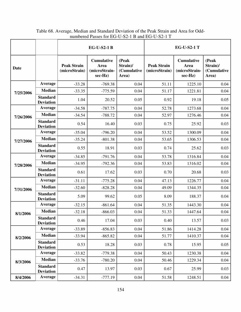
154
Table 68. Average, Median and Standard Deviation of the Peak Strain and Area for Odd-
numbered Passes for EG-U-S2-1 B and EG-U-S2-1 T
EG-U-S2-1 B
EG-U-S2-1 T
Date
Peak Strain (microStrain)
Cumulative
Area (microStrain-
sec-Hz)
(Peak
Strain)/
(Cumulative
Area)
Peak Strain (microStrain)
Cumulative
Area (microStrain-
sec-Hz)
(Peak
Strain)/
(Cumulative
Area)
7/25/2006
Average -33.28 -769.38 0.04 51.11 1225.10 0.04
Median -33.35 -775.59 0.04 51.17 1221.81 0.04
Standard
Deviation 1.04 20.52 0.05 0.92 19.18 0.05
7/26/2006
Average -34.58 -787.75 0.04 52.78 1273.68 0.04
Median -34.54 -788.72 0.04 52.97 1276.46 0.04
Standard
Deviation 0.54 16.40 0.03 0.75 25.92 0.03
7/27/2006
Average -35.04 -796.20 0.04 53.52 1300.09 0.04
Median -35.24 -801.38 0.04 53.65 1306.53 0.04
Standard
Deviation 0.55 18.91 0.03 0.74 25.62 0.03
7/28/2006
Average -34.85 -791.76 0.04 53.78 1316.84 0.04
Median -34.95 -792.36 0.04 53.83 1316.02 0.04
Standard
Deviation 0.61 17.62 0.03 0.70 20.68 0.03
7/31/2006
Average -31.11 -775.28 0.04 47.13 1226.77 0.04
Median -32.60 -828.28 0.04 49.09 1344.35 0.04
Standard
Deviation 5.09 99.62 0.05 8.09 188.37 0.04
8/1/2006
Average -32.15 -861.64 0.04 51.35 1443.30 0.04
Median -32.18 -866.03 0.04 51.33 1447.64 0.04
Standard
Deviation 0.46 17.04 0.03 0.40 13.57 0.03
8/2/2006
Average -33.89 -856.83 0.04 51.86 1414.28 0.04
Median -33.94 -865.82 0.04 51.77 1410.37 0.04
Standard
Deviation 0.53 18.28 0.03 0.78 15.95 0.05
8/3/2006
Average -33.82 -779.38 0.04 50.43 1230.38 0.04
Median -33.76 -780.20 0.04 50.46 1229.34 0.04
Standard
Deviation 0.47 13.97 0.03 0.67 25.99 0.03
8/4/2006 Average -34.31 -777.19 0.04 51.58 1248.51 0.04
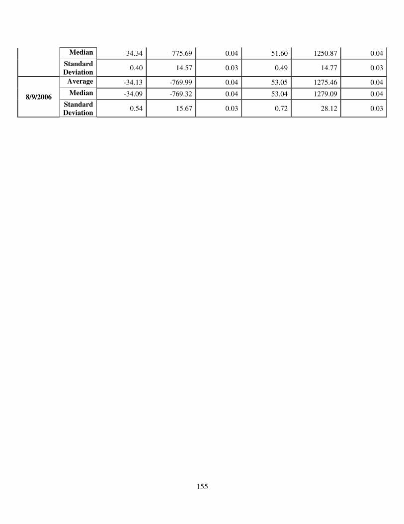
155
Median -34.34 -775.69 0.04 51.60 1250.87 0.04
Standard
Deviation 0.40 14.57 0.03 0.49 14.77 0.03
8/9/2006
Average -34.13 -769.99 0.04 53.05 1275.46 0.04
Median -34.09 -769.32 0.04 53.04 1279.09 0.04
Standard
Deviation 0.54 15.67 0.03 0.72 28.12 0.03
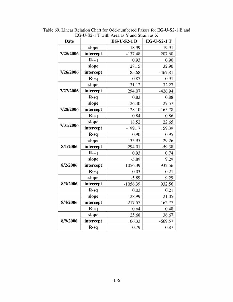
156
Table 69. Linear Relation Chart for Odd-numbered Passes for EG-U-S2-1 B and
EG-U-S2-1 T with Area as Y and Strain as X
Date EG-U-S2-1 B EG-U-S2-1 T
7/25/2006
slope 18.99 19.91
intercept -137.48 207.60
R-sq 0.93 0.90
7/26/2006
slope 28.15 32.90
intercept 185.68 -462.81
R-sq 0.87 0.91
7/27/2006
slope 31.12 32.27
intercept 294.07 -426.94
R-sq 0.83 0.88
7/28/2006
slope 26.40 27.57
intercept 128.10 -165.78
R-sq 0.84 0.86
7/31/2006
slope 18.52 22.65
intercept -199.17 159.39
R-sq 0.90 0.95
8/1/2006
slope 35.95 29.26
intercept 294.01 -59.38
R-sq 0.93 0.74
8/2/2006
slope -5.89 9.29
intercept -1056.39 932.56
R-sq 0.03 0.21
8/3/2006
slope -5.89 9.29
intercept -1056.39 932.56
R-sq 0.03 0.21
8/4/2006
slope 28.99 21.05
intercept 217.57 162.77
R-sq 0.64 0.48
8/9/2006
slope 25.68 36.67
intercept 106.33 -669.57
R-sq 0.79 0.87
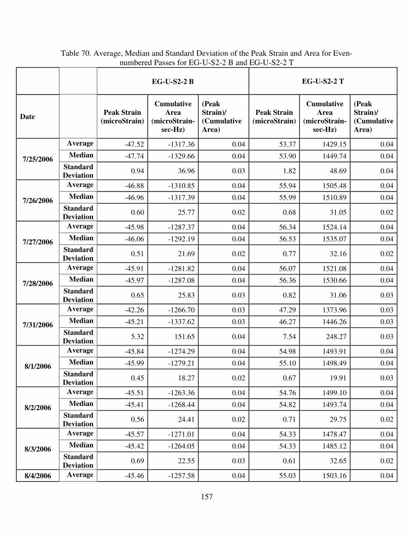
157
Table 70. Average, Median and Standard Deviation of the Peak Strain and Area for Even-
numbered Passes for EG-U-S2-2 B and EG-U-S2-2 T
EG-U-S2-2 B
EG-U-S2-2 T
Date
Peak Strain (microStrain)
Cumulative
Area (microStrain-
sec-Hz)
(Peak
Strain)/
(Cumulative
Area)
Peak Strain (microStrain)
Cumulative
Area (microStrain-
sec-Hz)
(Peak
Strain)/
(Cumulative
Area)
7/25/2006
Average -47.52 -1317.36 0.04 53.37 1429.15 0.04
Median -47.74 -1329.66 0.04 53.90 1449.74 0.04
Standard
Deviation 0.94 36.96 0.03 1.82 48.69 0.04
7/26/2006
Average -46.88 -1310.85 0.04 55.94 1505.48 0.04
Median -46.96 -1317.39 0.04 55.99 1510.89 0.04
Standard
Deviation 0.60 25.77 0.02 0.68 31.05 0.02
7/27/2006
Average -45.98 -1287.37 0.04 56.34 1524.14 0.04
Median -46.06 -1292.19 0.04 56.53 1535.07 0.04
Standard
Deviation 0.51 21.69 0.02 0.77 32.16 0.02
7/28/2006
Average -45.91 -1281.82 0.04 56.07 1521.08 0.04
Median -45.97 -1287.08 0.04 56.36 1530.66 0.04
Standard
Deviation 0.65 25.83 0.03 0.82 31.06 0.03
7/31/2006
Average -42.26 -1266.70 0.03 47.29 1373.96 0.03
Median -45.21 -1337.62 0.03 46.27 1446.26 0.03
Standard
Deviation 5.32 151.65 0.04 7.54 248.27 0.03
8/1/2006
Average -45.84 -1274.29 0.04 54.98 1493.91 0.04
Median -45.99 -1279.21 0.04 55.10 1498.49 0.04
Standard
Deviation 0.45 18.27 0.02 0.67 19.91 0.03
8/2/2006
Average -45.51 -1263.36 0.04 54.76 1499.10 0.04
Median -45.41 -1268.44 0.04 54.82 1493.74 0.04
Standard
Deviation 0.56 24.41 0.02 0.71 29.75 0.02
8/3/2006
Average -45.57 -1271.01 0.04 54.33 1478.47 0.04
Median -45.42 -1264.05 0.04 54.33 1485.12 0.04
Standard
Deviation 0.69 22.55 0.03 0.61 32.65 0.02
8/4/2006 Average -45.46 -1257.58 0.04 55.03 1503.16 0.04

158
Median -45.57 -1258.76 0.04 55.09 1501.68 0.04
Standard
Deviation 0.45 13.02 0.03 0.64 16.40 0.04
8/9/2006
Average -43.38 -1193.35 0.04 56.21 1556.73 0.04
Median -43.66 -1206.01 0.04 56.52 1567.60 0.04
Standard
Deviation 1.40 54.78 0.03 1.40 58.02 0.02
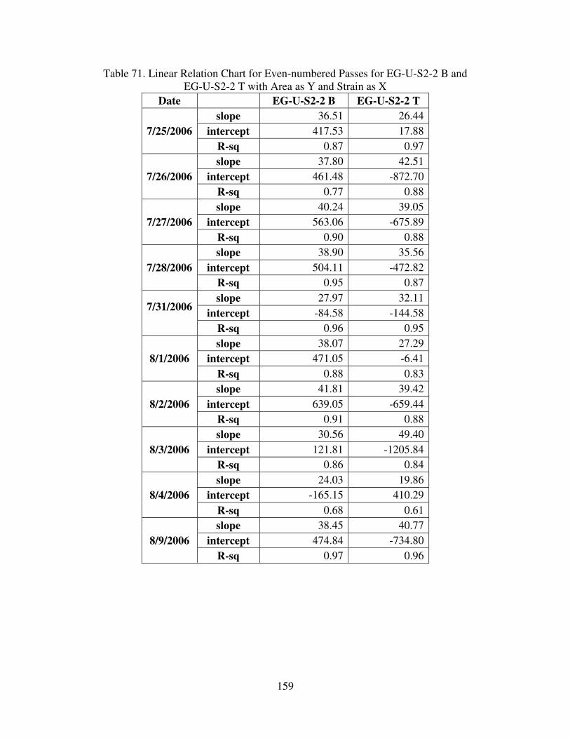
159
Table 71. Linear Relation Chart for Even-numbered Passes for EG-U-S2-2 B and
EG-U-S2-2 T with Area as Y and Strain as X
Date EG-U-S2-2 B EG-U-S2-2 T
7/25/2006
slope 36.51 26.44
intercept 417.53 17.88
R-sq 0.87 0.97
7/26/2006
slope 37.80 42.51
intercept 461.48 -872.70
R-sq 0.77 0.88
7/27/2006
slope 40.24 39.05
intercept 563.06 -675.89
R-sq 0.90 0.88
7/28/2006
slope 38.90 35.56
intercept 504.11 -472.82
R-sq 0.95 0.87
7/31/2006
slope 27.97 32.11
intercept -84.58 -144.58
R-sq 0.96 0.95
8/1/2006
slope 38.07 27.29
intercept 471.05 -6.41
R-sq 0.88 0.83
8/2/2006
slope 41.81 39.42
intercept 639.05 -659.44
R-sq 0.91 0.88
8/3/2006
slope 30.56 49.40
intercept 121.81 -1205.84
R-sq 0.86 0.84
8/4/2006
slope 24.03 19.86
intercept -165.15 410.29
R-sq 0.68 0.61
8/9/2006
slope 38.45 40.77
intercept 474.84 -734.80
R-sq 0.97 0.96

160
Table 72. Average, Median and Standard Deviation of the Peak Strain and Area for Odd-
numbered Passes for EG-U-N3-1 B and EG-U-N3-1 T
EG-U-N3-1 B
EG-U-N3-1 T
Date
Peak Strain (microStrain)
Cumulative
Area (microStrain-
sec-Hz)
(Peak
Strain)/
(Cumulative
Area)
Peak Strain (microStrain)
Cumulative
Area (microStrain-
sec-Hz)
(Peak
Strain)/
(Cumulative
Area)
7/25/2006
Average -15.90 -657.04 0.02 30.35 1141.07 0.03
Median -15.76 -651.72 0.02 30.48 1146.96 0.03
Standard
Deviation 0.57 19.53 0.03 0.34 19.95 0.02
7/26/2006
Average -14.55 -606.74 0.02 31.08 1179.65 0.03
Median -14.58 -612.40 0.02 31.07 1178.76 0.03
Standard
Deviation 0.73 32.44 0.02 0.27 11.44 0.02
7/27/2006
Average -13.31 -543.09 0.02 31.15 1199.07 0.03
Median -13.31 -545.55 0.02 31.08 1196.05 0.03
Standard
Deviation 0.26 20.17 0.01 0.37 15.23 0.02
7/28/2006
Average -12.59 -497.47 0.03 31.38 1218.86 0.03
Median -12.59 -500.74 0.03 31.32 1218.53 0.03
Standard
Deviation 0.37 16.25 0.02 0.30 12.05 0.02
7/31/2006
Average -9.70 -404.67 0.02 22.67 929.34 0.02
Median -11.33 -476.75 0.02 26.76 1087.10 0.02
Standard
Deviation 4.38 185.13 0.02 11.39 470.16 0.02
8/1/2006
Average -12.15 -460.68 0.03 31.70 1167.33 0.03
Median -12.16 -461.65 0.03 31.70 1168.88 0.03
Standard
Deviation 0.19 6.40 0.03 0.30 9.39 0.03

161
Table 73. Linear Relation Chart for Odd-numbered Passes for EG-U-N3-1 B and
EG-U-N3-1 T with Area as Y and Strain as X
Date EG-U-N3-1 B EG-U-N3-1 T
7/25/2006
slope 34.03 43.04
intercept -116.10 -165.09
R-sq 0.98 0.54
7/26/2006
slope 43.90 22.26
intercept 32.15 487.91
R-sq 0.98 0.28
7/27/2006
slope 66.06 36.48
intercept 336.49 62.89
R-sq 0.73 0.80
7/28/2006
slope 40.03 21.67
intercept 6.26 538.66
R-sq 0.83 0.29
7/31/2006
slope 41.61 41.07
intercept -1.02 -1.63
R-sq 0.97 0.99
8/1/2006
slope 27.81 8.87
intercept -122.90 886.14
R-sq 0.69 0.08

162
Table 74. Average, Median and Standard Deviation of the Peak Strain and Area for Even-
numbered Passes for EG-U-N3-2 B and EG-U-N3-2 T
EG-U-N3-2 B
EG-U-N3-2 T
Date
Peak Strain (microStrain)
Cumulative
Area (microStrain-
sec-Hz)
(Peak
Strain)/
(Cumulative
Area)
Peak Strain (microStrain)
Cumulative
Area (microStrain-
sec-Hz)
(Peak
Strain)/
(Cumulative
Area)
7/25/2006
Average -24.67 -1082.34 0.02 44.74 2190.27 0.02
Median -24.52 -1074.06 0.02 44.91 2197.32 0.02
Standard
Deviation 0.59 23.88 0.02 0.85 41.32 0.02
7/26/2006
Average -23.30 -1031.01 0.02 47.77 2371.51 0.02
Median -23.06 -1024.36 0.02 47.90 2365.05 0.02
Standard
Deviation 0.67 38.09 0.02 0.50 30.49 0.02
7/27/2006
Average -24.35 -1092.11 0.02 52.46 2627.69 0.02
Median -24.35 -1093.87 0.02 52.02 2599.74 0.02
Standard
Deviation 0.28 16.89 0.02 1.56 94.99 0.02
7/28/2006
Average -26.24 -1101.99 0.02 73.27 2833.57 0.03
Median -26.27 -1108.29 0.02 73.84 2882.51 0.03
Standard
Deviation 0.45 19.26 0.02 1.65 109.66 0.02
7/31/2006
Average -21.65 -1000.95 0.02 44.11 2196.31 0.02
Median -22.22 -990.91 0.02 49.94 2467.10 0.02
Standard
Deviation 1.27 84.45 0.02 12.98 707.94 0.02
8/1/2006
Average -25.51 -1162.32 0.02 57.58 2828.78 0.02
Median -25.49 -1160.81 0.02 57.63 2828.59 0.02
Standard
Deviation 0.23 7.58 0.03 0.38 12.14 0.03
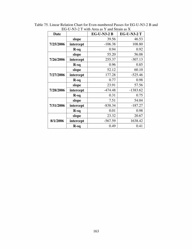
163
Table 75. Linear Relation Chart for Even-numbered Passes for EG-U-N3-2 B and
EG-U-N3-2 T with Area as Y and Strain as X
Date EG-U-N3-2 B EG-U-N3-2 T
7/25/2006
slope 39.56 46.53
intercept -106.38 108.80
R-sq 0.94 0.92
7/26/2006
slope 55.20 56.08
intercept 255.37 -307.13
R-sq 0.96 0.85
7/27/2006
slope 52.12 60.10
intercept 177.28 -525.46
R-sq 0.77 0.98
7/28/2006
slope 23.91 57.56
intercept -474.48 -1383.62
R-sq 0.31 0.75
7/31/2006
slope 7.51 54.04
intercept -838.34 -187.27
R-sq 0.01 0.98
8/1/2006
slope 23.32 20.67
intercept -567.59 1638.42
R-sq 0.49 0.41
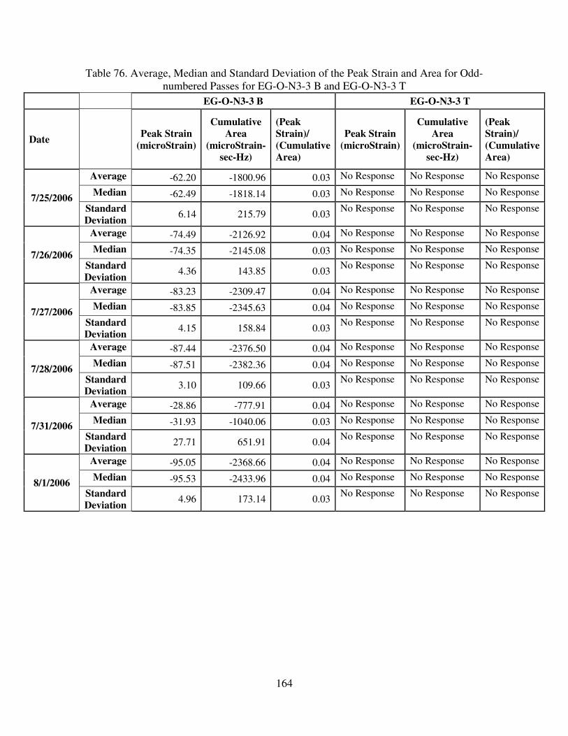
164
Table 76. Average, Median and Standard Deviation of the Peak Strain and Area for Odd-
numbered Passes for EG-O-N3-3 B and EG-O-N3-3 T
EG-O-N3-3 B EG-O-N3-3 T
Date
Peak Strain (microStrain)
Cumulative
Area (microStrain-
sec-Hz)
(Peak
Strain)/
(Cumulative
Area)
Peak Strain (microStrain)
Cumulative
Area (microStrain-
sec-Hz)
(Peak
Strain)/
(Cumulative
Area)
7/25/2006
Average -62.20 -1800.96 0.03 No Response No Response No Response
Median -62.49 -1818.14 0.03 No Response No Response No Response
Standard
Deviation 6.14 215.79 0.03
No Response No Response No Response
7/26/2006
Average -74.49 -2126.92 0.04 No Response No Response No Response
Median -74.35 -2145.08 0.03 No Response No Response No Response
Standard
Deviation 4.36 143.85 0.03
No Response No Response No Response
7/27/2006
Average -83.23 -2309.47 0.04 No Response No Response No Response
Median -83.85 -2345.63 0.04 No Response No Response No Response
Standard
Deviation 4.15 158.84 0.03
No Response No Response No Response
7/28/2006
Average -87.44 -2376.50 0.04 No Response No Response No Response
Median -87.51 -2382.36 0.04 No Response No Response No Response
Standard
Deviation 3.10 109.66 0.03
No Response No Response No Response
7/31/2006
Average -28.86 -777.91 0.04 No Response No Response No Response
Median -31.93 -1040.06 0.03 No Response No Response No Response
Standard
Deviation 27.71 651.91 0.04
No Response No Response No Response
8/1/2006
Average -95.05 -2368.66 0.04 No Response No Response No Response
Median -95.53 -2433.96 0.04 No Response No Response No Response
Standard
Deviation 4.96 173.14 0.03
No Response No Response No Response
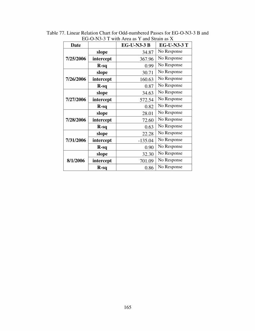
165
Table 77. Linear Relation Chart for Odd-numbered Passes for EG-O-N3-3 B and
EG-O-N3-3 T with Area as Y and Strain as X
Date EG-U-N3-3 B EG-U-N3-3 T
7/25/2006
slope 34.87 No Response
intercept 367.96 No Response
R-sq 0.99 No Response
7/26/2006
slope 30.71 No Response
intercept 160.63 No Response
R-sq 0.87 No Response
7/27/2006
slope 34.63 No Response
intercept 572.54 No Response
R-sq 0.82 No Response
7/28/2006
slope 28.01 No Response
intercept 72.60 No Response
R-sq 0.63 No Response
7/31/2006
slope 22.28 No Response
intercept -135.04 No Response
R-sq 0.90 No Response
8/1/2006
slope 32.30 No Response
intercept 701.09 No Response
R-sq 0.86 No Response

166
Table 78. Average, Median and Standard Deviation of the Peak Strain and Area for Even-
numbered Passes for EG-U-S3-1 B and EG-U-S3-1 T
EG-U-S3-1 B
EG-U-S3-1 T
Date
Peak Strain (microStrain)
Cumulative
Area (microStrain-
sec-Hz)
(Peak
Strain)/
(Cumulative
Area)
Peak Strain (microStrain)
Cumulative
Area (microStrain-
sec-Hz)
(Peak
Strain)/
(Cumulative
Area)
7/25/2006
Average -36.90 -988.81 0.04 61.20 1794.76 0.03
Median -36.95 -989.24 0.04 61.26 1809.08 0.03
Standard
Deviation 0.24 9.07 0.03 0.94 48.14 0.02
7/26/2006
Average -34.57 -934.61 0.04 63.28 1866.09 0.03
Median -34.50 -932.48 0.04 63.71 1869.31 0.03
Standard
Deviation 1.29 32.08 0.04 1.52 56.30 0.03
7/27/2006
Average -31.87 -885.01 0.04 64.68 1939.10 0.03
Median -31.96 -887.93 0.04 64.47 1915.75 0.03
Standard
Deviation 0.61 14.96 0.04 1.16 52.05 0.02
7/28/2006
Average -31.48 -883.61 0.04 65.53 1976.77 0.03
Median -31.53 -886.32 0.04 65.25 1965.86 0.03
Standard
Deviation 0.28 9.58 0.03 1.36 59.55 0.02
7/31/2006
Average -29.16 -871.67 0.03 59.79 1880.56 0.03
Median -29.43 -861.74 0.03 67.20 2075.70 0.03
Standard
Deviation 1.17 41.50 0.03 10.85 307.73 0.04
8/1/2006
Average -31.87 -916.42 0.03 67.49 2109.05 0.03
Median -31.88 -917.44 0.03 67.55 2104.13 0.03
Standard
Deviation 0.17 7.01 0.02 0.40 15.26 0.03
8/2/2006
Average -30.68 -880.82 0.03 69.39 2145.01 0.03
Median -30.66 -878.09 0.03 69.48 2147.35 0.03
Standard
Deviation 0.18 7.33 0.02 0.61 31.32 0.02
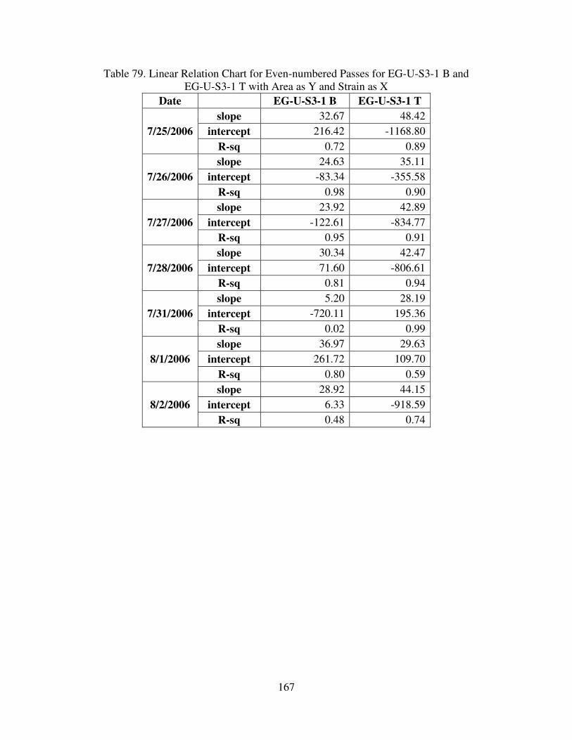
167
Table 79. Linear Relation Chart for Even-numbered Passes for EG-U-S3-1 B and
EG-U-S3-1 T with Area as Y and Strain as X
Date EG-U-S3-1 B EG-U-S3-1 T
7/25/2006
slope 32.67 48.42
intercept 216.42 -1168.80
R-sq 0.72 0.89
7/26/2006
slope 24.63 35.11
intercept -83.34 -355.58
R-sq 0.98 0.90
7/27/2006
slope 23.92 42.89
intercept -122.61 -834.77
R-sq 0.95 0.91
7/28/2006
slope 30.34 42.47
intercept 71.60 -806.61
R-sq 0.81 0.94
7/31/2006
slope 5.20 28.19
intercept -720.11 195.36
R-sq 0.02 0.99
8/1/2006
slope 36.97 29.63
intercept 261.72 109.70
R-sq 0.80 0.59
8/2/2006
slope 28.92 44.15
intercept 6.33 -918.59
R-sq 0.48 0.74
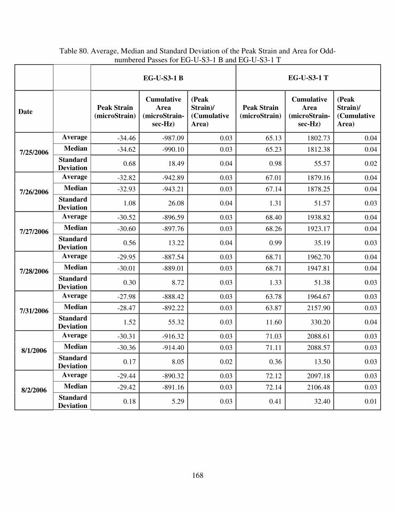
168
Table 80. Average, Median and Standard Deviation of the Peak Strain and Area for Odd-
numbered Passes for EG-U-S3-1 B and EG-U-S3-1 T
EG-U-S3-1 B
EG-U-S3-1 T
Date
Peak Strain (microStrain)
Cumulative
Area (microStrain-
sec-Hz)
(Peak
Strain)/
(Cumulative
Area)
Peak Strain (microStrain)
Cumulative
Area (microStrain-
sec-Hz)
(Peak
Strain)/
(Cumulative
Area)
7/25/2006
Average -34.46 -987.09 0.03 65.13 1802.73 0.04
Median -34.62 -990.10 0.03 65.23 1812.38 0.04
Standard
Deviation 0.68 18.49 0.04 0.98 55.57 0.02
7/26/2006
Average -32.82 -942.89 0.03 67.01 1879.16 0.04
Median -32.93 -943.21 0.03 67.14 1878.25 0.04
Standard
Deviation 1.08 26.08 0.04 1.31 51.57 0.03
7/27/2006
Average -30.52 -896.59 0.03 68.40 1938.82 0.04
Median -30.60 -897.76 0.03 68.26 1923.17 0.04
Standard
Deviation 0.56 13.22 0.04 0.99 35.19 0.03
7/28/2006
Average -29.95 -887.54 0.03 68.71 1962.70 0.04
Median -30.01 -889.01 0.03 68.71 1947.81 0.04
Standard
Deviation 0.30 8.72 0.03 1.33 51.38 0.03
7/31/2006
Average -27.98 -888.42 0.03 63.78 1964.67 0.03
Median -28.47 -892.22 0.03 63.87 2157.90 0.03
Standard
Deviation 1.52 55.32 0.03 11.60 330.20 0.04
8/1/2006
Average -30.31 -916.32 0.03 71.03 2088.61 0.03
Median -30.36 -914.40 0.03 71.11 2088.57 0.03
Standard
Deviation 0.17 8.05 0.02 0.36 13.50 0.03
8/2/2006
Average -29.44 -890.32 0.03 72.12 2097.18 0.03
Median -29.42 -891.16 0.03 72.14 2106.48 0.03
Standard
Deviation 0.18 5.29 0.03 0.41 32.40 0.01
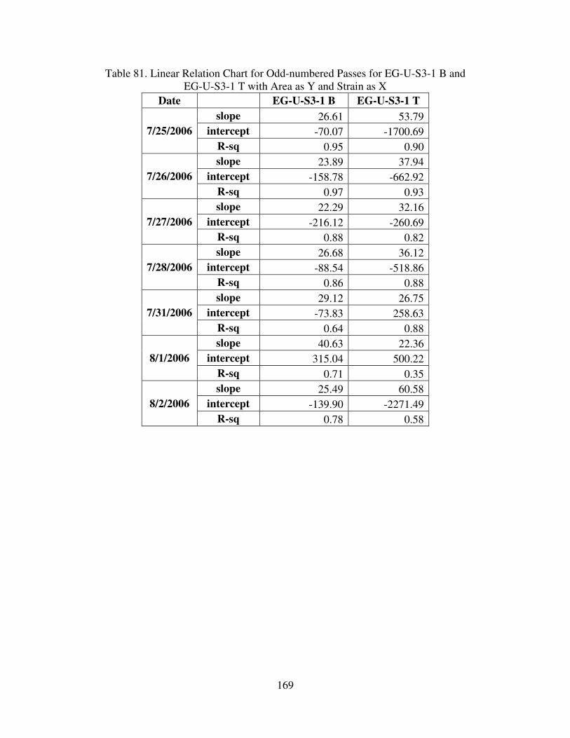
169
Table 81. Linear Relation Chart for Odd-numbered Passes for EG-U-S3-1 B and
EG-U-S3-1 T with Area as Y and Strain as X
Date EG-U-S3-1 B EG-U-S3-1 T
7/25/2006
slope 26.61 53.79
intercept -70.07 -1700.69
R-sq 0.95 0.90
7/26/2006
slope 23.89 37.94
intercept -158.78 -662.92
R-sq 0.97 0.93
7/27/2006
slope 22.29 32.16
intercept -216.12 -260.69
R-sq 0.88 0.82
7/28/2006
slope 26.68 36.12
intercept -88.54 -518.86
R-sq 0.86 0.88
7/31/2006
slope 29.12 26.75
intercept -73.83 258.63
R-sq 0.64 0.88
8/1/2006
slope 40.63 22.36
intercept 315.04 500.22
R-sq 0.71 0.35
8/2/2006
slope 25.49 60.58
intercept -139.90 -2271.49
R-sq 0.78 0.58
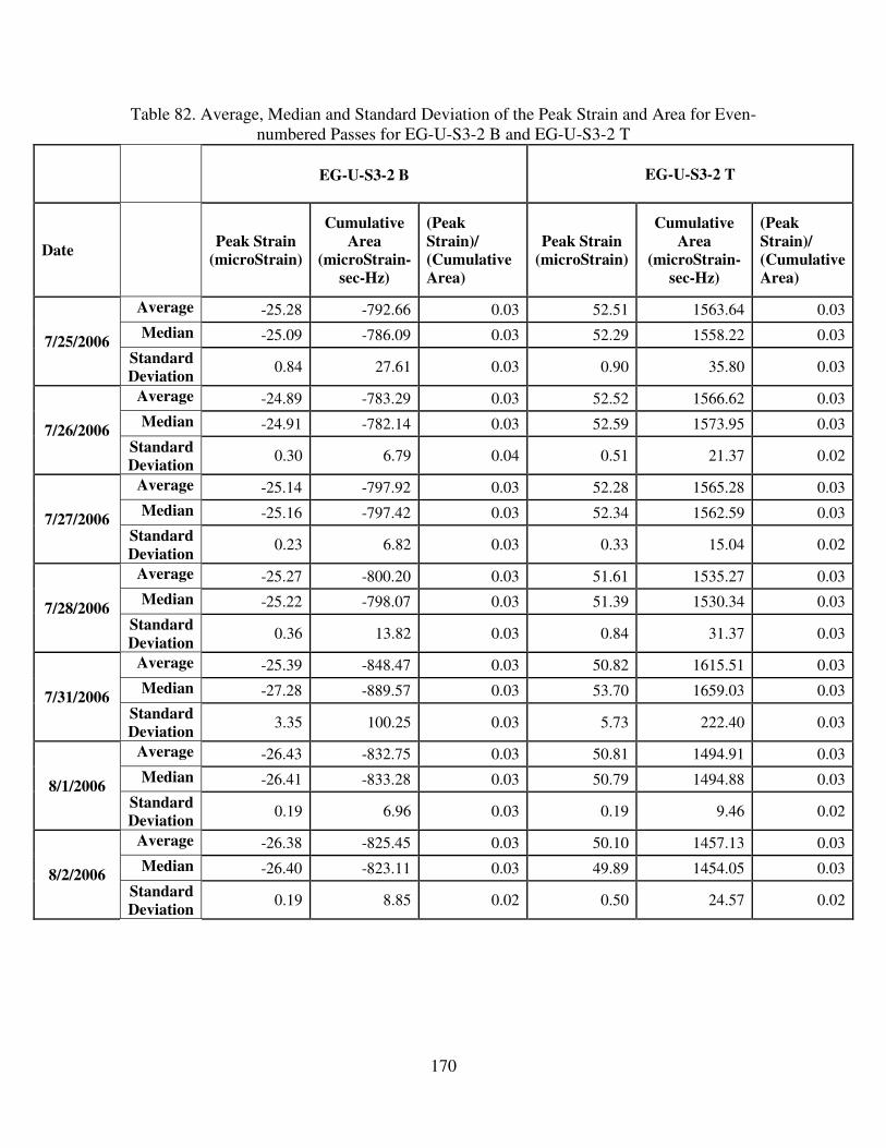
170
Table 82. Average, Median and Standard Deviation of the Peak Strain and Area for Even-
numbered Passes for EG-U-S3-2 B and EG-U-S3-2 T
EG-U-S3-2 B
EG-U-S3-2 T
Date
Peak Strain (microStrain)
Cumulative
Area (microStrain-
sec-Hz)
(Peak
Strain)/
(Cumulative
Area)
Peak Strain (microStrain)
Cumulative
Area (microStrain-
sec-Hz)
(Peak
Strain)/
(Cumulative
Area)
7/25/2006
Average -25.28 -792.66 0.03 52.51 1563.64 0.03
Median -25.09 -786.09 0.03 52.29 1558.22 0.03
Standard
Deviation 0.84 27.61 0.03 0.90 35.80 0.03
7/26/2006
Average -24.89 -783.29 0.03 52.52 1566.62 0.03
Median -24.91 -782.14 0.03 52.59 1573.95 0.03
Standard
Deviation 0.30 6.79 0.04 0.51 21.37 0.02
7/27/2006
Average -25.14 -797.92 0.03 52.28 1565.28 0.03
Median -25.16 -797.42 0.03 52.34 1562.59 0.03
Standard
Deviation 0.23 6.82 0.03 0.33 15.04 0.02
7/28/2006
Average -25.27 -800.20 0.03 51.61 1535.27 0.03
Median -25.22 -798.07 0.03 51.39 1530.34 0.03
Standard
Deviation 0.36 13.82 0.03 0.84 31.37 0.03
7/31/2006
Average -25.39 -848.47 0.03 50.82 1615.51 0.03
Median -27.28 -889.57 0.03 53.70 1659.03 0.03
Standard
Deviation 3.35 100.25 0.03 5.73 222.40 0.03
8/1/2006
Average -26.43 -832.75 0.03 50.81 1494.91 0.03
Median -26.41 -833.28 0.03 50.79 1494.88 0.03
Standard
Deviation 0.19 6.96 0.03 0.19 9.46 0.02
8/2/2006
Average -26.38 -825.45 0.03 50.10 1457.13 0.03
Median -26.40 -823.11 0.03 49.89 1454.05 0.03
Standard
Deviation 0.19 8.85 0.02 0.50 24.57 0.02
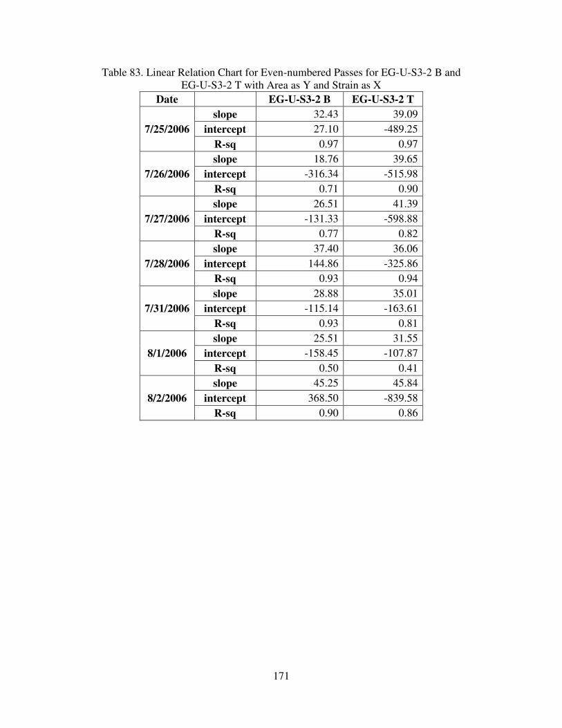
171
Table 83. Linear Relation Chart for Even-numbered Passes for EG-U-S3-2 B and
EG-U-S3-2 T with Area as Y and Strain as X
Date EG-U-S3-2 B EG-U-S3-2 T
7/25/2006
slope 32.43 39.09
intercept 27.10 -489.25
R-sq 0.97 0.97
7/26/2006
slope 18.76 39.65
intercept -316.34 -515.98
R-sq 0.71 0.90
7/27/2006
slope 26.51 41.39
intercept -131.33 -598.88
R-sq 0.77 0.82
7/28/2006
slope 37.40 36.06
intercept 144.86 -325.86
R-sq 0.93 0.94
7/31/2006
slope 28.88 35.01
intercept -115.14 -163.61
R-sq 0.93 0.81
8/1/2006
slope 25.51 31.55
intercept -158.45 -107.87
R-sq 0.50 0.41
8/2/2006
slope 45.25 45.84
intercept 368.50 -839.58
R-sq 0.90 0.86
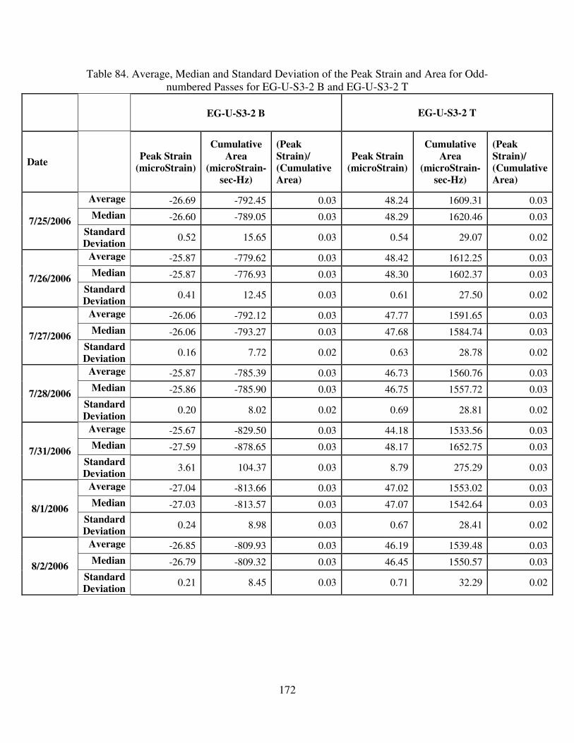
172
Table 84. Average, Median and Standard Deviation of the Peak Strain and Area for Odd-
numbered Passes for EG-U-S3-2 B and EG-U-S3-2 T
EG-U-S3-2 B
EG-U-S3-2 T
Date
Peak Strain (microStrain)
Cumulative
Area (microStrain-
sec-Hz)
(Peak
Strain)/
(Cumulative
Area)
Peak Strain (microStrain)
Cumulative
Area (microStrain-
sec-Hz)
(Peak
Strain)/
(Cumulative
Area)
7/25/2006
Average -26.69 -792.45 0.03 48.24 1609.31 0.03
Median -26.60 -789.05 0.03 48.29 1620.46 0.03
Standard
Deviation 0.52 15.65 0.03 0.54 29.07 0.02
7/26/2006
Average -25.87 -779.62 0.03 48.42 1612.25 0.03
Median -25.87 -776.93 0.03 48.30 1602.37 0.03
Standard
Deviation 0.41 12.45 0.03 0.61 27.50 0.02
7/27/2006
Average -26.06 -792.12 0.03 47.77 1591.65 0.03
Median -26.06 -793.27 0.03 47.68 1584.74 0.03
Standard
Deviation 0.16 7.72 0.02 0.63 28.78 0.02
7/28/2006
Average -25.87 -785.39 0.03 46.73 1560.76 0.03
Median -25.86 -785.90 0.03 46.75 1557.72 0.03
Standard
Deviation 0.20 8.02 0.02 0.69 28.81 0.02
7/31/2006
Average -25.67 -829.50 0.03 44.18 1533.56 0.03
Median -27.59 -878.65 0.03 48.17 1652.75 0.03
Standard
Deviation 3.61 104.37 0.03 8.79 275.29 0.03
8/1/2006
Average -27.04 -813.66 0.03 47.02 1553.02 0.03
Median -27.03 -813.57 0.03 47.07 1542.64 0.03
Standard
Deviation 0.24 8.98 0.03 0.67 28.41 0.02
8/2/2006
Average -26.85 -809.93 0.03 46.19 1539.48 0.03
Median -26.79 -809.32 0.03 46.45 1550.57 0.03
Standard
Deviation 0.21 8.45 0.03 0.71 32.29 0.02
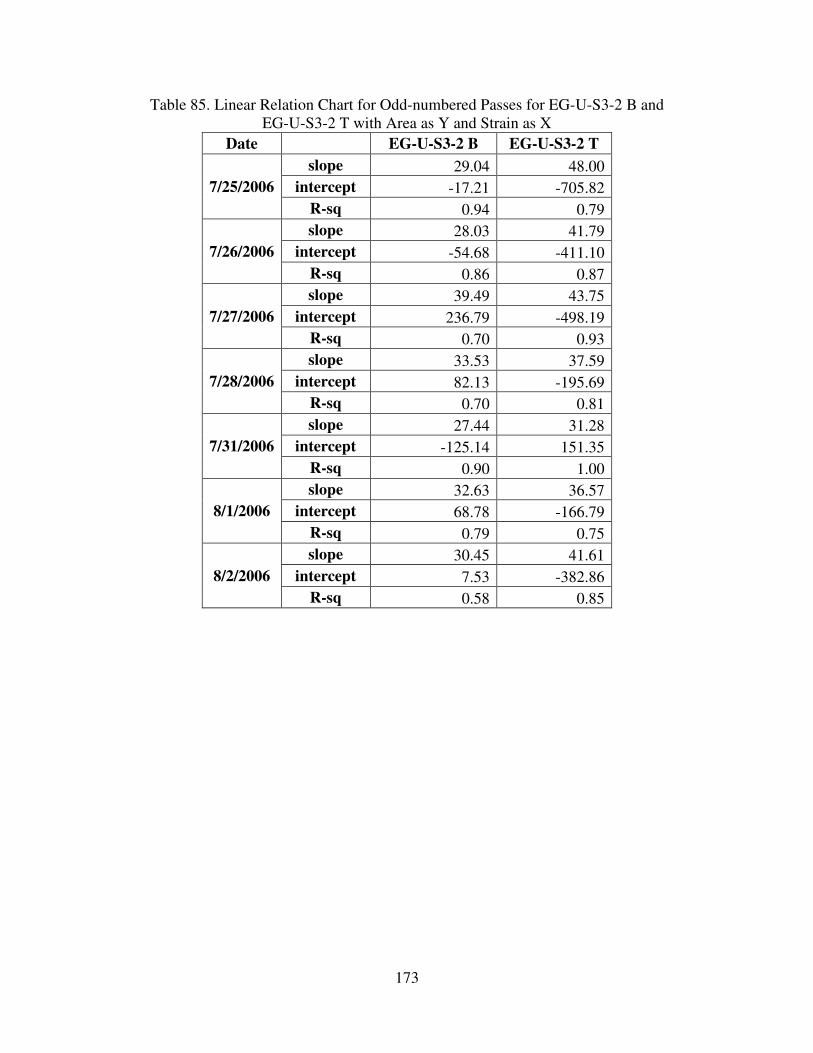
173
Table 85. Linear Relation Chart for Odd-numbered Passes for EG-U-S3-2 B and
EG-U-S3-2 T with Area as Y and Strain as X
Date EG-U-S3-2 B EG-U-S3-2 T
7/25/2006
slope 29.04 48.00
intercept -17.21 -705.82
R-sq 0.94 0.79
7/26/2006
slope 28.03 41.79
intercept -54.68 -411.10
R-sq 0.86 0.87
7/27/2006
slope 39.49 43.75
intercept 236.79 -498.19
R-sq 0.70 0.93
7/28/2006
slope 33.53 37.59
intercept 82.13 -195.69
R-sq 0.70 0.81
7/31/2006
slope 27.44 31.28
intercept -125.14 151.35
R-sq 0.90 1.00
8/1/2006
slope 32.63 36.57
intercept 68.78 -166.79
R-sq 0.79 0.75
8/2/2006
slope 30.45 41.61
intercept 7.53 -382.86
R-sq 0.58 0.85
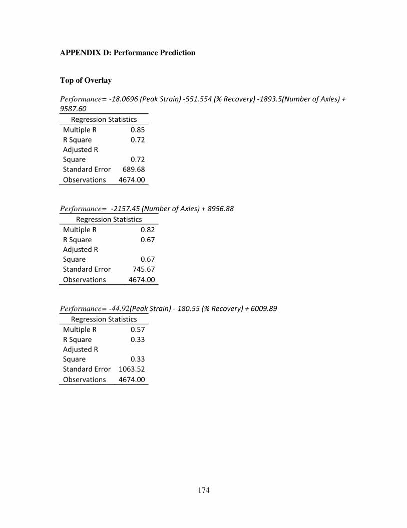
174
APPENDIX D: Performance Prediction
Top of Overlay
Performance= -18.0696 (Peak Strain) -551.554 (% Recovery) -1893.5(Number of Axles) +
9587.60
Regression Statistics
Multiple R 0.85
R Square 0.72
Adjusted R
Square 0.72
Standard Error 689.68
Observations 4674.00
Performance= -2157.45 (Number of Axles) + 8956.88
Regression Statistics
Multiple R 0.82
R Square 0.67
Adjusted R
Square 0.67
Standard Error 745.67
Observations 4674.00
Performance= -44.92(Peak Strain) - 180.55 (% Recovery) + 6009.89
Regression Statistics
Multiple R 0.57
R Square 0.33
Adjusted R
Square 0.33
Standard Error 1063.52
Observations 4674.00
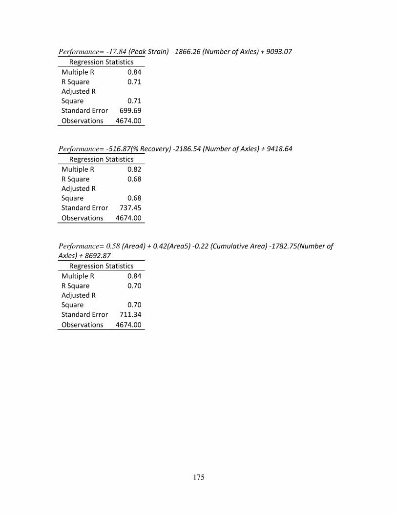
175
Performance= -17.84 (Peak Strain) -1866.26 (Number of Axles) + 9093.07
Regression Statistics
Multiple R 0.84
R Square 0.71
Adjusted R
Square 0.71
Standard Error 699.69
Observations 4674.00
Performance= -516.87(% Recovery) -2186.54 (Number of Axles) + 9418.64
Regression Statistics
Multiple R 0.82
R Square 0.68
Adjusted R
Square 0.68
Standard Error 737.45
Observations 4674.00
Performance= 0.58 (Area4) + 0.42(Area5) -0.22 (Cumulative Area) -1782.75(Number of
Axles) + 8692.87
Regression Statistics
Multiple R 0.84
R Square 0.70
Adjusted R
Square 0.70
Standard Error 711.34
Observations 4674.00
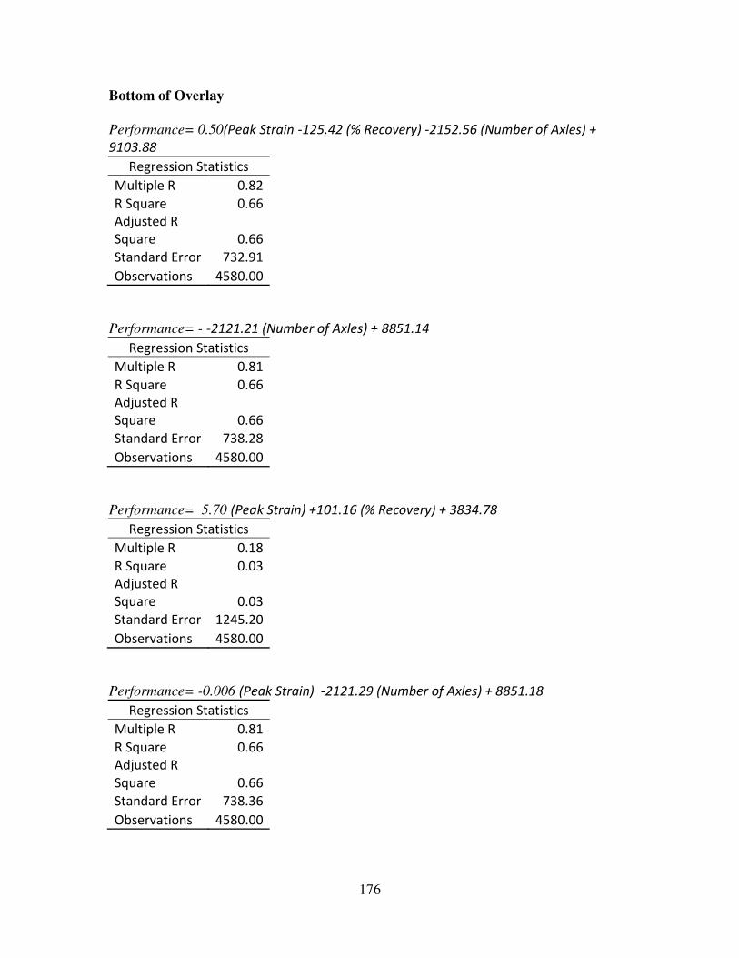
176
Bottom of Overlay
Performance= 0.50(Peak Strain -125.42 (% Recovery) -2152.56 (Number of Axles) +
9103.88
Regression Statistics
Multiple R 0.82
R Square 0.66
Adjusted R
Square 0.66
Standard Error 732.91
Observations 4580.00
Performance= - -2121.21 (Number of Axles) + 8851.14
Regression Statistics
Multiple R 0.81
R Square 0.66
Adjusted R
Square 0.66
Standard Error 738.28
Observations 4580.00
Performance= 5.70 (Peak Strain) +101.16 (% Recovery) + 3834.78
Regression Statistics
Multiple R 0.18
R Square 0.03
Adjusted R
Square 0.03
Standard Error 1245.20
Observations 4580.00
Performance= -0.006 (Peak Strain) -2121.29 (Number of Axles) + 8851.18
Regression Statistics
Multiple R 0.81
R Square 0.66
Adjusted R
Square 0.66
Standard Error 738.36
Observations 4580.00
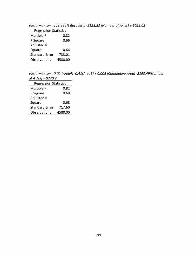
177
Performance= -121.24 (% Recovery) -2158.53 (Number of Axles) + 9099.05
Regression Statistics
Multiple R 0.82
R Square 0.66
Adjusted R
Square 0.66
Standard Error 733.01
Observations 4580.00
Performance= -0.05 (Area4) -0.41(Area5) + 0.005 (Cumulative Area) -2193.49(Number
of Axles) + 9240.2
Regression Statistics
Multiple R 0.82
R Square 0.68
Adjusted R
Square 0.68
Standard Error 717.60
Observations 4580.00
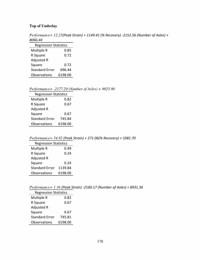
178
Top of Underlay
Performance= 12.25(Peak Strain) + 1149.41 (% Recovery) -2152.56 (Number of Axles) +
8066.44
Regression Statistics
Multiple R 0.85
R Square 0.72
Adjusted R
Square 0.72
Standard Error 696.44
Observations 6198.00
Performance= -2177.29 (Number of Axles) + 9025.90
Regression Statistics
Multiple R 0.82
R Square 0.67
Adjusted R
Square 0.67
Standard Error 745.84
Observations 6198.00
Performance= 54.92 (Peak Strain) + 271.06(% Recovery) + 1081.70
Regression Statistics
Multiple R 0.49
R Square 0.24
Adjusted R
Square 0.24
Standard Error 1139.84
Observations 6198.00
Performance= 1.16 (Peak Strain) -2160.17 (Number of Axles) + 8931.36
Regression Statistics
Multiple R 0.82
R Square 0.67
Adjusted R
Square 0.67
Standard Error 745.81
Observations 6198.00
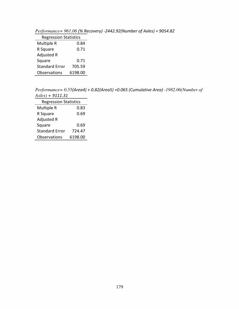
179
Performance= 961.06 (% Recovery) -2442.92(Number of Axles) + 9054.82
Regression Statistics
Multiple R 0.84
R Square 0.71
Adjusted R
Square 0.71
Standard Error 705.59
Observations 6198.00
Performance= 0.55(Area4) + 0.82(Area5) +0.065 (Cumulative Area) -1982.06(Number of
Axles) + 9111.31
Regression Statistics
Multiple R 0.83
R Square 0.69
Adjusted R
Square 0.69
Standard Error 724.47
Observations 6198.00
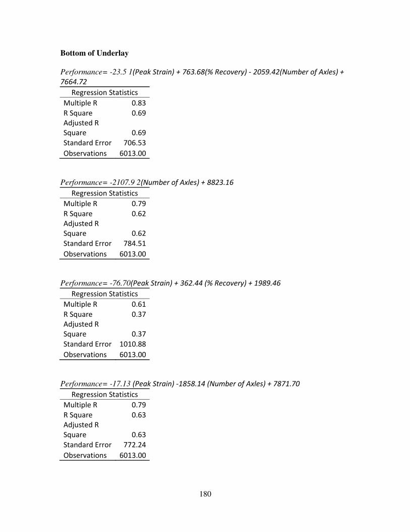
180
Bottom of Underlay
Performance= -23.5 1(Peak Strain) + 763.68(% Recovery) - 2059.42(Number of Axles) +
7664.72
Regression Statistics
Multiple R 0.83
R Square 0.69
Adjusted R
Square 0.69
Standard Error 706.53
Observations 6013.00
Performance= -2107.9 2(Number of Axles) + 8823.16
Regression Statistics
Multiple R 0.79
R Square 0.62
Adjusted R
Square 0.62
Standard Error 784.51
Observations 6013.00
Performance= -76.70(Peak Strain) + 362.44 (% Recovery) + 1989.46
Regression Statistics
Multiple R 0.61
R Square 0.37
Adjusted R
Square 0.37
Standard Error 1010.88
Observations 6013.00
Performance= -17.13 (Peak Strain) -1858.14 (Number of Axles) + 7871.70
Regression Statistics
Multiple R 0.79
R Square 0.63
Adjusted R
Square 0.63
Standard Error 772.24
Observations 6013.00
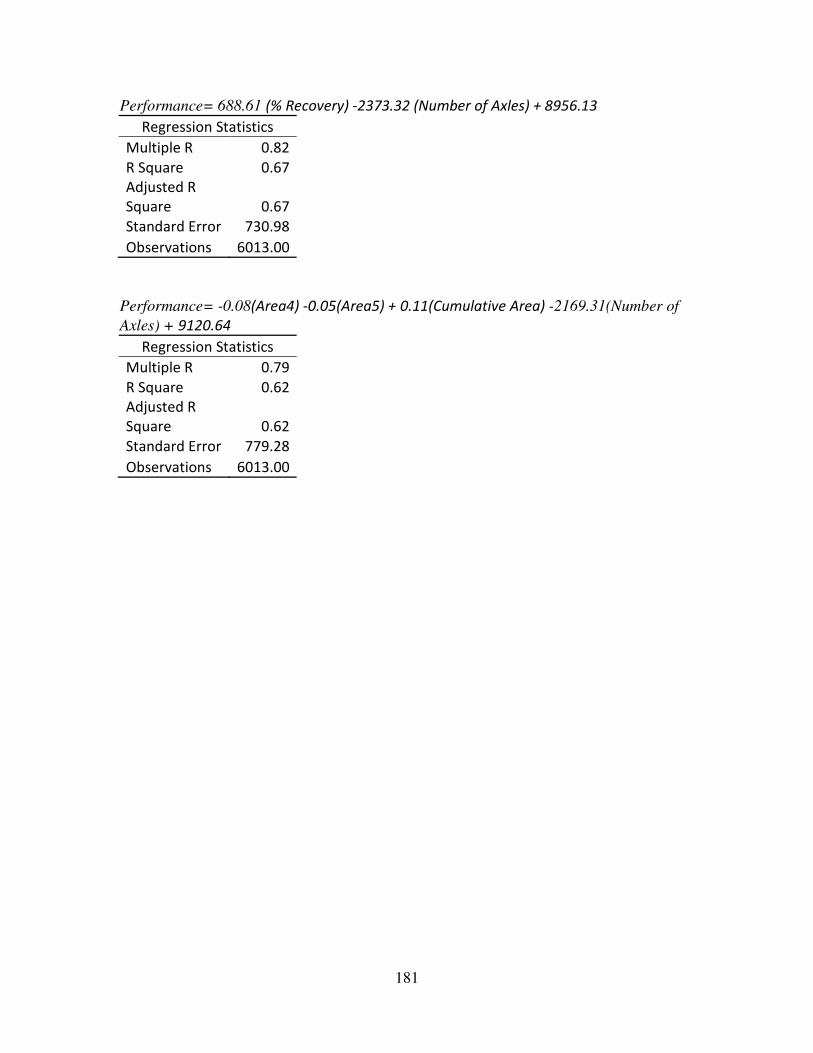
181
Performance= 688.61 (% Recovery) -2373.32 (Number of Axles) + 8956.13
Regression Statistics
Multiple R 0.82
R Square 0.67
Adjusted R
Square 0.67
Standard Error 730.98
Observations 6013.00
Performance= -0.08(Area4) -0.05(Area5) + 0.11(Cumulative Area) -2169.31(Number of
Axles) + 9120.64
Regression Statistics
Multiple R 0.79
R Square 0.62
Adjusted R
Square 0.62
Standard Error 779.28
Observations 6013.00