CONTRIBUTED RESEARCH ARTICLES 7

stplanr: A Package for Transport Planningby Robin Lovelace, Richard Ellison

Abstract Tools for transport planning should be flexible, scalable, and transparent. The stplanrpackage demonstrates and provides a home for such tools, with an emphasis on spatial transportdata and non-motorized modes. The stplanr package facilitates common transport planning tasksincluding: downloading and cleaning transport datasets; creating geographic “desire lines” fromorigin-destination (OD) data; route assignment, locally and interfaces to routing services such asCycleStreets.net; calculation of route segment attributes such as bearing and aggregate flow; and‘travel watershed’ analysis. This paper demonstrates this functionality using reproducible exampleson real transport datasets. More broadly, the experience of developing and using R functions fortransport applications shows that open source software can form the basis of a reproducible transportplanning workflow. The stplanr package, alongside other packages and open source projects, couldprovide a more transparent and democratically accountable alternative to the current approach, whichis heavily reliant on proprietary and relatively inaccessible software.

Introduction

Transport planning can broadly be defined as the process of designing and evaluating transportinterventions (Ortuzar and Willumsen, 2011), usually with the ultimate aim of improving transportsystems from economic, social, and environmental perspectives. This inevitably involves a degreeof subjective judgment and intuition. With the proliferation of new transport datasets — and theincreasing availability of hardware and software to make sense of them — there is great potential forthe discipline to become more evidence-based and scientific (Balmer et al., 2009). Transport plannershave always undertaken a wide range of computational activities (Boyce and Williams, 2015), but withthe digital revolution the demands have grown beyond the capabilities of a single, monolithic product.The diversity of tasks, and the need for democratic accountability in public decision making, suggeststhat future-proof transport planning software should be:

• flexible, able to handle a wide range of data formats• scalable, able to work at multiple geographic levels from single streets to large cities and regions• robust and reliable, tested on a range of datasets and able to work “out of the box” in a range of

real-world projects• open source and reproducible, ensuring transparency and encouraging citizen science

This paper sets out to demonstrate that open source software with a command-line interface (CLI)can provide a foundation for transport planning software that meets each of these criteria. R providesa strong basis for progress in this direction because it already contains functionality used in commontransport planning workflows. The sp, rgeos, and rgdal packages greatly improved R’s spatial abilities(Bivand et al., 2013), work that is being consolidated and extended in the recent sf package.

Building on these foundations, a number of spatial packages have been developed for applieddomains including: disease mapping and modelling, with packages such as SpatialEpi and dis-easemapping (Kim and Wakefield, 2016; Brown and Zhou, 2016); spatial ecology, with the adehabitatfamily of packages (Calenge, 2006); and visualisation, with packages such as leaflet, tmap, mapview,and mapmisc (Brown, 2016). However, there has been little prior work to develop R functionalitydesigned specifically for transport planning, with the notable exceptions of TravelR (a package onR-Forge last updated in 2012) and gtfsr (a package for handling General Transit Feed Specification(GTFS) data).

The purpose of stplanr is to provide a toolbox rather than a specific solution for transport planning,with an emphasis on spatial data and active modes. This emphasis is timely given the recent emphasison sustainability (Banister, 2008) and ‘Big Data’ (Zheng et al., 2016) in the wider field of transportplanning.

A major motivation was the lack of R packages, and open source software in general, for transportapplications. This may be surprising given the ubiquity of transport problems;1 R’s proficiency athandling spatial, temporal and travel survey data that describe transport systems; and the growingpopularity of R in applied domains (Jalal et al.; Moore and Hutchinson). Another motivation is thegrowth in open access datasets: the main purpose of early versions of the package was to process openorigin-destination data (Lovelace et al., 2017).

1Many people can think of things that could be improved on their local transport networks, especially forwalking, cycling and wheel-chairs, but most lack the evidence to communicate the issues, and potential solutions,to others.

The R Journal Vol. 10/2, December 2018 ISSN 2073-4859

CONTRIBUTED RESEARCH ARTICLES 8

R is already used in transport applications, as illustrated by recent research that applies packagesfrom other domains to transport problems. For instance, Efthymiou and Antoniou (2012) use R toanalyse the data collected from an online survey focused on car-sharing, bicycle-sharing, and electricvehicles. Efthymiou and Antoniou (2012) also used R to collect and analyse transport-related data fromTwitter using packages including XML, twitteR and ggplot2. These packages were used to download,parse and plot the Twitter data using a method that can be repeated and the results reproduced orupdated. More general statistical analyses have also been conducted on transport-related datasetsusing packages including muStat and mgcv (Diana, 2012; Cerin et al., 2013). Despite the rising use ofR for transport research, there has yet been to be a package for transport planning.

The design of the R language, with its emphasis on flexibility, data processing, and statisticalmodelling, suggests it can provide a powerful environment for transport planning research. Thereare many quantitative methods in transport planning, many of which fit into the classic ‘four stage’transport model which involves the following steps (Ortuzar and Willumsen, 2011): (1) trip generationto estimate trip frequency from origins; (2) distribution of trips to destinations; (3) modal split of tripsbetween walking, cycling, buses etc.; (4) assignment of trips to the transport route network. To thiswe would like to add two more stages for the big data age: (0) data processing and exploration; and(5) validation. This sequence is not the only way of transport modelling and some have argued thatits dominance has reduced innovation. However it is certainly a common approach and provides auseful schema for classifying the kinds of task that stplanr can tackle:

• accessing and processing of data on transport infrastructure and behaviour (stage 0)• analysis and visualisation of the transport network (0)• analysis of origin-destination (OD) data and the visualisation of resulting ‘desire lines’• the allocation of desire lines to roads and other guideways via routing services• the aggregation of routes to estimate total levels of flow on segments throughout the transport

network• development of models to estimate transport behaviour currently and under various scenarios

of change• the calculation of “catchment areas” affected by transport infrastructure

The automation of such tasks can assist researchers and practitioners to create evidence for decisionmaking. If the data processing and analysis stages are fast and painless, more time can be dedicated tovisualisation and decision making. This should allow researchers to focus on problems, rather than onclunky graphical user interfaces (GUIs), and ad-hoc scripts that could be generalised. Furthermore, ifthe process can be made reproducible and accessible (e.g. via online visualisation packages such asshiny), this could help transport planning move away from reliance on “black boxes” (Waddell, 2002)and empower citizens to challenge decisions made by transport planning authorities based on theevidence (Hollander, 2016).

There are many advantages of using a scriptable, interactive, and open source language such as Rfor transport planning. Such an approach enables: reproducible research; the automation and sharingof code between researchers; reduced barriers to innovation, as anyone can create new features for thebenefit of all planners; easier interaction with non domain experts (who will lack dedicated software);and integration with other software systems, as illustrated by the use of leaflet to generate JavaScriptfor sharing interactive maps for transport planning, used in the publicly accessible Propensity to CycleTool (Lovelace et al., 2017). Furthermore, R has a strong user community which can support newcomers(stplanr was peer reviewed thanks to the community surrounding ROpenSci). The advantages ofusing R specifically to develop the functionality described in this paper are that it has excellent geo-statistical capabilities (Pebesma et al., 2015), visualisation packages (e.g. tmap, ggplot2), support forlogit models (which are useful for modelling modal shift), and support for the many formats thattransport datasets are stored in (e.g., via the haven and rio packages).

Package structure and functionality

The package can be installed and attached as follows (see the package’s README for dependenciesand access to development versions):

install.packages("stplanr")

library(stplanr)

stplanr imports both sp and its successor sf. This means that spatial objects used in and producedby the package work with base R generic functions such as summary, aggregate, and plot (Bivandet al., 2013). Furthermore, output objects of class "sf" are mostly compatible with the popular dataprocessing package dplyr.

The R Journal Vol. 10/2, December 2018 ISSN 2073-4859

CONTRIBUTED RESEARCH ARTICLES 9

Core functions and classes

The package’s core functions are structured around three common types of spatial transport data:

• Origin-destination (OD) data, which report the number of people travelling between origin-destination pairs. This type of data is not explicitly spatial (OD datasets are usually representedas data frames) but represents movement over space between points in geographical space. Anexample is provided in the flow dataset.

• Line data, one dimensional linear features on the surface of the Earth. These are typically storedas a "SpatialLinesDataFrame" object.

• Route data are special types of lines which have been allocated to the transport network. Routestypically result from the allocation of a straight “desire line” allocated to the route network witha route_ function. Route network represent many overlapping routes. All are typically storedas a "SpatialLinesDataFrame" object.

A convention has been developed whereby function names are prefixed depending on the theinput data type (od_, line_ and route_ respectively, although route_ functions do not take routes asinputs, they output them). A selection of these is presented in Table 1 (lsf.str("package:stplanr")returns a list of all functions). Additional “core functions” could be developed, such as those prefixedwith rn_ (for working with route network data) and geo_ functions for geographic operations such asbuffer creation on lat/lon projected data (this function is currently named buff_geo).

Function Input data type(s) Output data type

od_dist Data frame Numeric vectorod_id_order Data frame Data frameline_bearing Spatial line Numeric vectorline_midpoint Spatial line Spatial pointsroute_cyclestreet Coordinates, spatial point or text Spatial linesroute_graphhopper Coordinates, spatial point or text Spatial lines

Table 1: Selection of functions for working with or generating OD, line and route data types.

We aim to preserve type in some functions: line2route, for example, takes spatial lines objectsand returns spatial lines objects. Type stability has its limitations with spatial data, however: it wouldbe wasteful for functions such as line_bearing (which returns the bearing of a line) to duplicate thespatial data contained in its input, for instance. Generic classes enable stplanr to handle objects ofclass "sf" from the new sf package in a type preserving way.

A class system has not been developed for each data type (this option is discussed in the finalsection) and more classes would be possible: transport datasets are diverse. This diversity helpsexplain why some functions have more ad-hoc names. Rather than attempting a systematic descriptionof each of stplanr’s functions, the remainder of this paper shows how the package can be used fortransport planning, beginning with data access and ending with visualisation.

Road traffic casualty data

Gaining access to data is often the problem in transport planning. It can be a long and protractedprocess but is becoming easier thanks to the “open data” movement and packages such as tigris andosmdata (Walker, 2016).

The stplanr package helps import data with functions including read_table_builder, for im-porting data from the Australian Bureau of Statistics (ABS), and dl_stats19 — which has now beensplit-out into the package stats19 — for downloading datasets from the UK’s Stats19 road trafficcasualty system (Lovelace et al., 2019). A brief example of the latter is demonstrated below, whichbegins with downloading the data (warning this downloads ~100 MB of data):

dl_stats19() # download and extract stats19 road traffic casualty data

#> [1] "Data saved at: /tmp/RtmpppF3E2/Accidents0514.csv"#> [2] "Data saved at: /tmp/RtmpppF3E2/Casualties0514.csv"#> [3] "Data saved at: /tmp/RtmpppF3E2/Vehicles0514.csv"

Once the data has been saved in the default directory, determined by tempdir, it can be read-inand cleaned with the read_stats19_ functions (note these call format_stats19_ functions internallyto clean the datasets and add correct labels to the variables):

The R Journal Vol. 10/2, December 2018 ISSN 2073-4859

CONTRIBUTED RESEARCH ARTICLES 10

ac <- read_stats19_ac()ca <- read_stats19_ca()ve <- read_stats19_ve()

The resulting datasets (representing accident, casualty, and vehicle level data, respectively) can bemerged and made geographic, as illustrated below:2

library(dplyr)ca_ac <- inner_join(ca, ac)ca_fatal <- ca_ac %>%filter(Casualty_Severity == "Fatal" & !is.na(Latitude)) %>%select(Age = Age_of_Casualty, Mode = Casualty_Type, Longitude, Latitude)

ca_sp <- sp::SpatialPointsDataFrame(coords = ca_cycle[3:4], data = ca_cycle[1:2])

Now that this casualty data has been cleaned, subsetted (to only include fatal crashes) andconverted into a spatial class system, we can analyse the data using geographical datasets of thetype commonly used by stplanr. The following code, for example, geographically subsets the datasetto include only crashes that occurred within the bounding box of a sample route network datasetcontained as a dataset in stplanr for illustrative purposes. Note the use of bb2poly, which converts aspatial dataset into a box, represented as a rectangular SpatialPolygonsDataFrame:

data("route_network")sp::proj4string(ca_sp) <- sp::proj4string(route_network)bb <- bb2poly(route_network)sp::proj4string(bb) <- sp::proj4string(route_network)ca_local <- ca_sp[bb,]

The above code chunk shows the importance of understanding geographical data when workingwith transport data. It is only by converting the casualty data into a spatial data class, and adding acoordinate reference system (CRS), that transport planners and researchers can link this importantdataset back to the route network. We can now perform GIS operations on the results. The next codechunk, for example, finds all the fatalities that took place within 100 m of the route network, using thefunction buff_geo:

rnet_buff_100 <- buff_geo(route_network, width = 100)ca_buff <- ca_local[rnet_buff_100,]

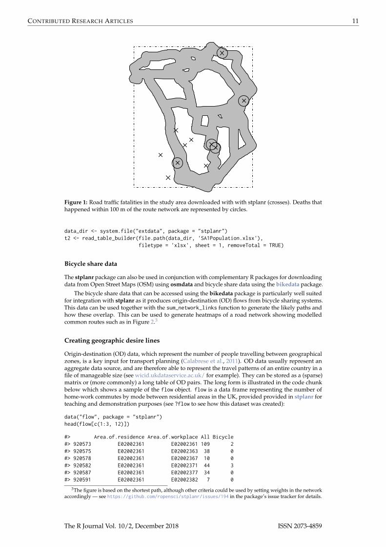
These can be visualised using base R graphics, extended by sp, as illustrated in Figure 1. Thisprovides a good start for analysis but for publication-quality plots and interactive plots, designed forpublic engagement, we recommend using dedicated visualisation packages that work with spatialdata such as tmap.

plot(bb, lty = 4)plot(rnet_buff_100, col = "grey", add = TRUE)points(ca_local, pch = 4)points(ca_buff, cex = 3)

Reading census data

National censuses are one common source of transport data, that frequently include questions onwhere people live and work. This is often accompanied by a question on what mode was taken. Thesedata are generally provided in standard tables that can be downloaded for free. For the Australiancensus, both these standard tables are available as well as custom tables that can be produced using aservice named TableBuilder. TableBuilder generates Excel or CSV files that contain additional linesthat make reading these data into R difficult. The stplanr package provides the read_table_builderfunction to read in these files.

Using the example SA1Population.xlsx file included with stplanr that contains the populationby SA1 zone (a statistical area used for the Australian census), we can use the read_table_builderfunction to read and format the table for use in R. The function automatically removes the additionallines and sets the column headers and data types as appropriate. The result is a data frame that can beused with GIS boundary files and other datasets produced for SA1 zones.

2Note the inner_join function from the dplyr package was used because it is substantially faster and moreeffective than the equivalent function, merge, in base R. This is communicated in a number of places, including onthe website zevross.com. For this reason we import dplyr and use it internally for joins.

The R Journal Vol. 10/2, December 2018 ISSN 2073-4859

CONTRIBUTED RESEARCH ARTICLES 11

Figure 1: Road traffic fatalities in the study area downloaded with with stplanr (crosses). Deaths thathappened within 100 m of the route network are represented by circles.

data_dir <- system.file("extdata", package = "stplanr")t2 <- read_table_builder(file.path(data_dir, 'SA1Population.xlsx'),

filetype = 'xlsx', sheet = 1, removeTotal = TRUE)

Bicycle share data

The stplanr package can also be used in conjunction with complementary R packages for downloadingdata from Open Street Maps (OSM) using osmdata and bicycle share data using the bikedata package.

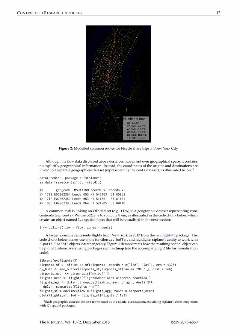
The bicycle share data that can be accessed using the bikedata package is particularly well suitedfor integration with stplanr as it produces origin-destination (OD) flows from bicycle sharing systems.This data can be used together with the sum_network_links function to generate the likely paths andhow these overlap. This can be used to generate heatmaps of a road network showing modelledcommon routes such as in Figure 2.3

Creating geographic desire lines

Origin-destination (OD) data, which represent the number of people travelling between geographicalzones, is a key input for transport planning (Calabrese et al., 2011). OD data usually represent anaggregate data source, and are therefore able to represent the travel patterns of an entire country in afile of manageable size (see wicid.ukdataservice.ac.uk/ for example). They can be stored as a (sparse)matrix or (more commonly) a long table of OD pairs. The long form is illustrated in the code chunkbelow which shows a sample of the flow object. flow is a data frame representing the number ofhome-work commutes by mode between residential areas in the UK, provided provided in stplanr forteaching and demonstration purposes (see ?flow to see how this dataset was created):

data("flow", package = "stplanr")head(flow[c(1:3, 12)])

#> Area.of.residence Area.of.workplace All Bicycle#> 920573 E02002361 E02002361 109 2#> 920575 E02002361 E02002363 38 0#> 920578 E02002361 E02002367 10 0#> 920582 E02002361 E02002371 44 3#> 920587 E02002361 E02002377 34 0#> 920591 E02002361 E02002382 7 0

3The figure is based on the shortest path, although other criteria could be used by setting weights in the networkaccordingly — see https://github.com/ropensci/stplanr/issues/194 in the package’s issue tracker for details.

The R Journal Vol. 10/2, December 2018 ISSN 2073-4859

CONTRIBUTED RESEARCH ARTICLES 12

Figure 2: Modelled common routes for bicycle share trips in New York City.

Although the flow data displayed above describes movement over geographical space, it containsno explicitly geographical information. Instead, the coordinates of the origins and destinations arelinked to a separate geographical dataset (represented by the cents dataset), as illustrated below:4

data("cents", package = "stplanr")as.data.frame(cents[1:3, -c(3,4)])

#> geo_code MSOA11NM coords.x1 coords.x2#> 1708 E02002384 Leeds 055 -1.546463 53.80952#> 1712 E02002382 Leeds 053 -1.511861 53.81161#> 1805 E02002393 Leeds 064 -1.524205 53.80410

A common task is linking an OD dataset (e.g., flow) to a geographic dataset representing zonecentroids (e.g. cents). We use od2line to combine them, as illustrated in the code chunk below, whichcreates an object named l, a spatial object that will be visualised in the next section:

l <- od2line(flow = flow, zones = cents)

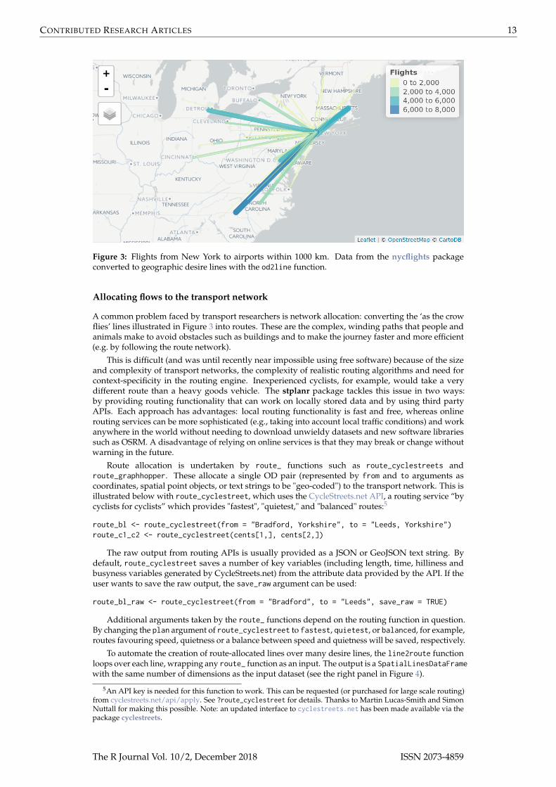
A larger example represents flights from New York in 2013 from the nycflights13 package. Thecode chunk below makes use of the function geo_buffer, and highlights stplanr’s ability to work with"Spatial" or "sf" objects interchangeably. Figure 3 demonstrates how the resulting spatial object canbe plotted interactively using packages such as tmap (see the accompanying R file for visualisationcode).

library(nycflights13)airports_sf <- sf::st_as_sf(airports, coords = c("lon", "lat"), crs = 4326)ny_buff <- geo_buffer(airports_sf[airports_sf$faa == "NYC",], dist = 1e6)airports_near <- airports_sf[ny_buff,]flights_near <- flights[flights$dest %in% airports_near$faa,]flights_agg <- dplyr::group_by(flights_near, origin, dest) %>%dplyr::summarise(Flights = n())

flights_sf = od2line(flow = flights_agg, zones = airports_near)plot(flights_sf, lwd = flights_sf$Flights / 1e3)

4Such geographic datasets are best represented as in a spatial class system, explaining stplanr’s close integrationwith R’s spatial packages.

The R Journal Vol. 10/2, December 2018 ISSN 2073-4859

CONTRIBUTED RESEARCH ARTICLES 13

Figure 3: Flights from New York to airports within 1000 km. Data from the nycflights packageconverted to geographic desire lines with the od2line function.

Allocating flows to the transport network

A common problem faced by transport researchers is network allocation: converting the ‘as the crowflies’ lines illustrated in Figure 3 into routes. These are the complex, winding paths that people andanimals make to avoid obstacles such as buildings and to make the journey faster and more efficient(e.g. by following the route network).

This is difficult (and was until recently near impossible using free software) because of the sizeand complexity of transport networks, the complexity of realistic routing algorithms and need forcontext-specificity in the routing engine. Inexperienced cyclists, for example, would take a verydifferent route than a heavy goods vehicle. The stplanr package tackles this issue in two ways:by providing routing functionality that can work on locally stored data and by using third partyAPIs. Each approach has advantages: local routing functionality is fast and free, whereas onlinerouting services can be more sophisticated (e.g., taking into account local traffic conditions) and workanywhere in the world without needing to download unwieldy datasets and new software librariessuch as OSRM. A disadvantage of relying on online services is that they may break or change withoutwarning in the future.

Route allocation is undertaken by route_ functions such as route_cyclestreets androute_graphhopper. These allocate a single OD pair (represented by from and to arguments ascoordinates, spatial point objects, or text strings to be "geo-coded") to the transport network. This isillustrated below with route_cyclestreet, which uses the CycleStreets.net API, a routing service “bycyclists for cyclists” which provides "fastest", "quietest," and "balanced" routes:5

route_bl <- route_cyclestreet(from = "Bradford, Yorkshire", to = "Leeds, Yorkshire")route_c1_c2 <- route_cyclestreet(cents[1,], cents[2,])

The raw output from routing APIs is usually provided as a JSON or GeoJSON text string. Bydefault, route_cyclestreet saves a number of key variables (including length, time, hilliness andbusyness variables generated by CycleStreets.net) from the attribute data provided by the API. If theuser wants to save the raw output, the save_raw argument can be used:

route_bl_raw <- route_cyclestreet(from = "Bradford", to = "Leeds", save_raw = TRUE)

Additional arguments taken by the route_ functions depend on the routing function in question.By changing the plan argument of route_cyclestreet to fastest, quietest, or balanced, for example,routes favouring speed, quietness or a balance between speed and quietness will be saved, respectively.

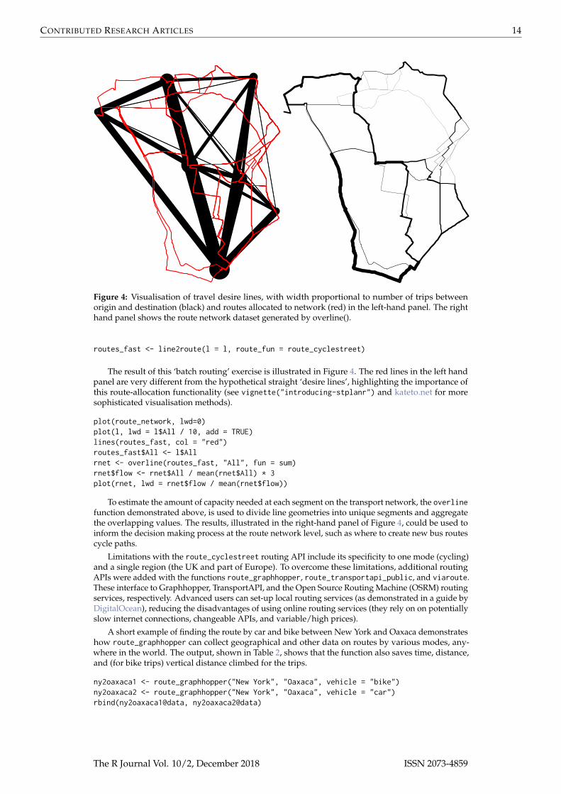
To automate the creation of route-allocated lines over many desire lines, the line2route functionloops over each line, wrapping any route_ function as an input. The output is a SpatialLinesDataFramewith the same number of dimensions as the input dataset (see the right panel in Figure 4).

5An API key is needed for this function to work. This can be requested (or purchased for large scale routing)from cyclestreets.net/api/apply. See ?route_cyclestreet for details. Thanks to Martin Lucas-Smith and SimonNuttall for making this possible. Note: an updated interface to cyclestreets.net has been made available via thepackage cyclestreets.

The R Journal Vol. 10/2, December 2018 ISSN 2073-4859

CONTRIBUTED RESEARCH ARTICLES 14

Figure 4: Visualisation of travel desire lines, with width proportional to number of trips betweenorigin and destination (black) and routes allocated to network (red) in the left-hand panel. The righthand panel shows the route network dataset generated by overline().

routes_fast <- line2route(l = l, route_fun = route_cyclestreet)

The result of this ‘batch routing’ exercise is illustrated in Figure 4. The red lines in the left handpanel are very different from the hypothetical straight ‘desire lines’, highlighting the importance ofthis route-allocation functionality (see vignette("introducing-stplanr") and kateto.net for moresophisticated visualisation methods).

plot(route_network, lwd=0)plot(l, lwd = l$All / 10, add = TRUE)lines(routes_fast, col = "red")routes_fast$All <- l$Allrnet <- overline(routes_fast, "All", fun = sum)rnet$flow <- rnet$All / mean(rnet$All) * 3plot(rnet, lwd = rnet$flow / mean(rnet$flow))

To estimate the amount of capacity needed at each segment on the transport network, the overlinefunction demonstrated above, is used to divide line geometries into unique segments and aggregatethe overlapping values. The results, illustrated in the right-hand panel of Figure 4, could be used toinform the decision making process at the route network level, such as where to create new bus routescycle paths.

Limitations with the route_cyclestreet routing API include its specificity to one mode (cycling)and a single region (the UK and part of Europe). To overcome these limitations, additional routingAPIs were added with the functions route_graphhopper, route_transportapi_public, and viaroute.These interface to Graphhopper, TransportAPI, and the Open Source Routing Machine (OSRM) routingservices, respectively. Advanced users can set-up local routing services (as demonstrated in a guide byDigitalOcean), reducing the disadvantages of using online routing services (they rely on on potentiallyslow internet connections, changeable APIs, and variable/high prices).

A short example of finding the route by car and bike between New York and Oaxaca demonstrateshow route_graphhopper can collect geographical and other data on routes by various modes, any-where in the world. The output, shown in Table 2, shows that the function also saves time, distance,and (for bike trips) vertical distance climbed for the trips.

ny2oaxaca1 <- route_graphhopper("New York", "Oaxaca", vehicle = "bike")ny2oaxaca2 <- route_graphhopper("New York", "Oaxaca", vehicle = "car")rbind(ny2oaxaca1@data, ny2oaxaca2@data)

The R Journal Vol. 10/2, December 2018 ISSN 2073-4859

CONTRIBUTED RESEARCH ARTICLES 15

mode time dist change_elev

Bike 17522.73 4885663 87388.13Car 2759.89 4754772 NA

Table 2: Results obtained from the Graphhopper API using the route_graphhopper function to es-timate the time taken and route distance to travel between New York and Oaxaca by cycling anddriving.

Modelling travel catchment areas

Catchment areas are useful analytic and visual tools in transport planning. They can help who willbenefit from a particular transport intervention (such as a new bus stop) and illustrate the geographicarea that is covered by (or omitted from) a particular service or transport system, to help prioritizenew investment. Passengers are often said to be willing to walk up to 400 metres to a bus stop or 800metres to a railway station (El-Geneidy et al., 2014), leading to surrounding smaller or larger polygonsrepresenting the catchment within which people would be willing to travel. Such catchment areas havebeen criticised as being arbitrary or as underestimating the true sphere of influence of public transportnodes (El-Geneidy et al., 2014; Daniels and Mulley, 2013). However, they nonetheless represent agood starting point from which the geographical and social distribution of service provision can beestimated.

Often catchment areas are calculated using straight-line (or “as the crow flies”) distances. Thisapproach is appealing because it requires little additional data and is simple to compute (using bufferfunction) and understand.

The stplanr package provides functionality that calculates catchment areas using straight-linedistances with the calc_catchment function. This function takes a "SpatialPolygonsDataFrame"object that contains the population (or other) data, typically from a census, and a Spatial* layer thatcontains the geometry of the transport facility. These two layers are overlayed to calculate statisticsfor the desired catchments including "proportioning" polygons to account for the proportion locatedwithin the catchment area.

To illustrate this functionality, the following code chunk reads-in sample datasets stored in thecommon ESRI Shapefile format using the readOGR function from rgdal. The resulting object smallsa1contains population data for Statistical Area 1 (SA1) zones in Sydney, Australia. The testcyclewaydata set contains hypothetical cycleways aligned to streets in Sydney:

data_dir <- system.file("extdata", package = "stplanr")unzip(file.path(data_dir, 'smallsa1.zip'))unzip(file.path(data_dir, 'testcycleway.zip'))sa1income <- rgdal::readOGR(".", "smallsa1")testcycleway <- rgdal::readOGR(".", "testcycleway")# Remove unzipped filesfile.remove(list.files(pattern = "^(smallsa1|testcycleway).*"))

The calculation of catchment areas requires two parameters: a vector containing column names tocalculate statistics and a distance. Since proportioning the areas assumes projected data, unprojecteddata are automatically projected to either a common projection (if one is already projected) or aspecified projection. It should be emphasized that the choice of projection is important and has aneffect on the results meaning setting a local projection is recommended to achieve the most accurateresults. The catchment area is calculated as follows:

catch800m <- calc_catchment(polygonlayer = sa1income,targetlayer = testcycleway,calccols = c('Total'),distance = 800,projection = 'austalbers',dissolve = TRUE

)

The result can be used to calculate the total population within the catchment areas of the cycleway,with the command ‘sum(catch800m$Total)’: 39418 people. The catchment area can then be visualised(see Figure 5):

The R Journal Vol. 10/2, December 2018 ISSN 2073-4859

CONTRIBUTED RESEARCH ARTICLES 16

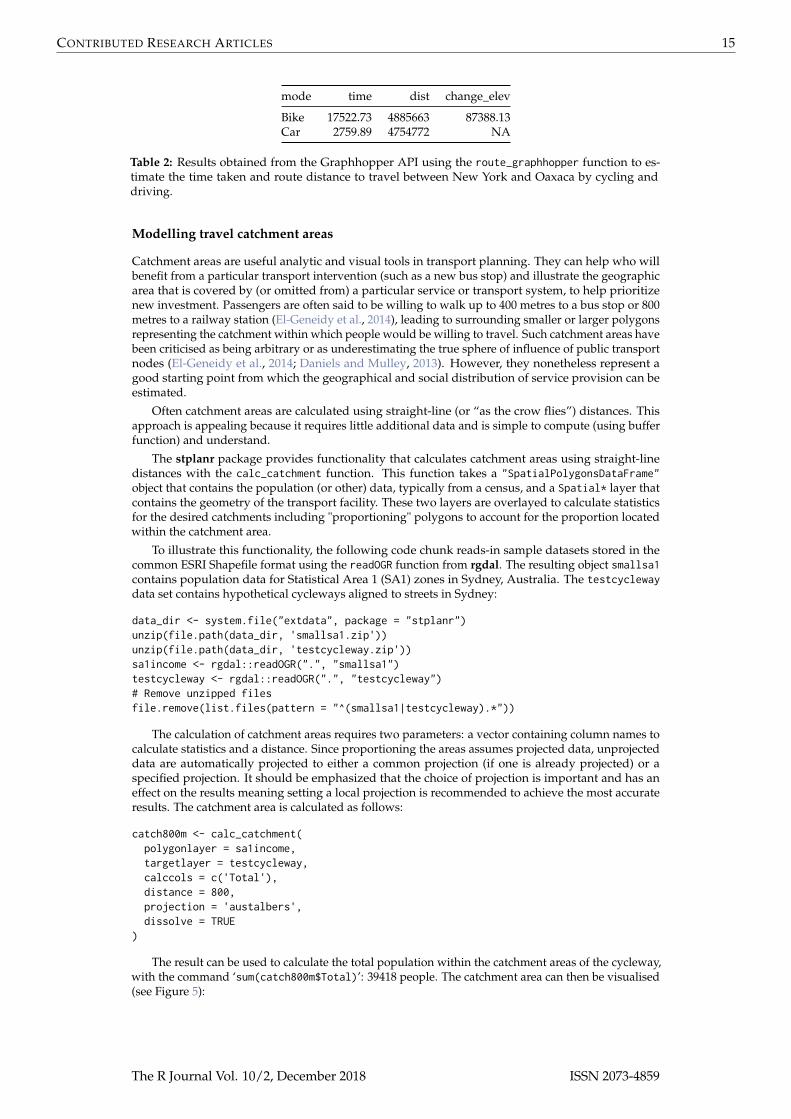
Figure 5: An 800 metre catchment area (red) associated with a cycle path (green) using straight-linedistance in Sydney.

plot(sa1income, col = "light grey")plot(catch800m, col = rgb(1, 0, 0, 0.5), add = TRUE)plot(testcycleway, col = "green", add = TRUE)

This simplistic catchment area is useful when the straight-line distance is a reasonable approxima-tion of the route taken to walk (or cycle) to a transport facility. However, this is often not the case. Thecatchment area in Figure 5 initially appears reasonable but the red-shaded catchment area includesan area that requires travelling around a bay to access from the (green-coloured) cycleway: usersmay have access but that does not mean it’s accessible. To allow for more realistic catchment areas formost situations, stplanr provides the calc_network_catchment function that uses the same principleas calc_catchment but also takes into account the transport network.

To use calc_network_catchment, a transport network, as a "SpatialLinesNetwork" object, mustbe provided. This combines a "SpatialLinesDataFrame" object with a graph network (using theigraph package) to allow routing (estimation of shortest paths). The network is used to calculate theshortest actual paths within the specific catchment distance, as demonstrated in the following codechunk:

unzip(file.path(data_dir, 'sydroads.zip'))sydroads <- rgdal::readOGR(".", "roads")file.remove(list.files(pattern = "^(roads).*"))sydnetwork <- SpatialLinesNetwork(sydroads)

The network catchment is then calculated using a similar method as with calc_catchment butwith a few minor changes. Specifically these are including the SpatialLinesNetwork, and using themaximpedance parameter to define the distance, with distance being the additional distance fromthe network. In contrast to the distance parameter that is based on the straight-line distance inboth the calc_catchment and calc_network_catchment functions, the maximpedance parameter is themaximum value in the units of the network’s weight attribute. In practice this is generally distance inmetres but can also be travel times, risk or other measures.

netcatch800m <- calc_network_catchment(sln = sydnetwork,polygonlayer = sa1income,targetlayer = testcycleway,calccols = c('Total'),maximpedance = 800,distance = 100,projection = 'austalbers'

)

Once calculated, the network catchment area can be used just as the straight-line network catch-ment. This includes extracting the catchment population of 23457 and plotting the original catchment

The R Journal Vol. 10/2, December 2018 ISSN 2073-4859

CONTRIBUTED RESEARCH ARTICLES 17

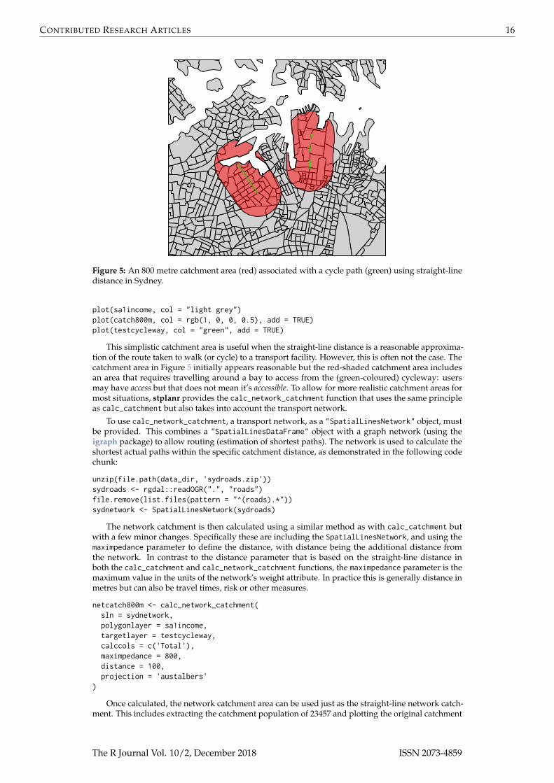
Figure 6: A 800 metre network catchment are (blue) compared with a catchment area based onEuclidean distance (red) associated with a cycle path (green).

area together with the original area with the results shown in Figure 6:

plot(sa1income, col = "light grey")plot(catch800m, col = rgb(1, 0, 0, 0.5), add = TRUE)plot(netcatch800m, col = rgb(0, 0, 1, 0.5), add = TRUE)plot(testcycleway, col = "green", add = TRUE)

The calc_catchment and calc_network_catchment functions are complementary functions allow-ing for the computation of catchment areas. Although for many transport applications it would bebetter to use the calc_network_catchment function that uses the true network distances, it may stillbe useful to use the straight-line version in some cases. These include calculating the population thatmay be affected by noise levels from transport infrastructure (such as a motorway) where the effectsof noise are not limited by the network. In situations where network data is not available it would bepossible to use the calc_catchment function together with a fixed assumption about what straight-linedistance corresponds to the desired network distance (i.e., 1km network = 700m straight-line). It mayalso be appropriate to use the straight-line distance when the network is not a reasonable constraint.This may be because the infrastructure of interest is accessed primarily by walking or cycling in an areawhere these are not limited to the road network (such as parks or shopping areas with passthroughsor overpasses available to pedestrians).

Modelling and visualisation

Analysing mode use

Route-allocated lines allow estimation of route distance and therefore circuity (Q) (route distance dividedby Euclidean distance) (Levinson and El-Geneidy, 2009):

Q =dR f

dE,

where (dE) and (dR f ) represent Euclidean and fastest route distance respectively.

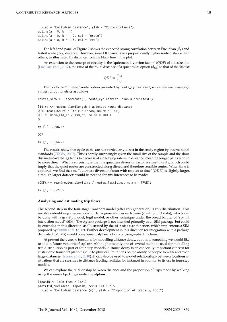
These variables can help model the rate of flow between origins and destination, as illustrated inthe left-hand panel of Figure 7. The code below demonstrates how objects generated by stplanr can beused to undertake such analysis, with the line_length function used to find the distance, in meters,of lat/lon data.

l$d_euclidean <- line_length(l)l$d_rf <- routes_fast@data$lengthplot(l$d_euclidean, l$d_rf,

The R Journal Vol. 10/2, December 2018 ISSN 2073-4859

CONTRIBUTED RESEARCH ARTICLES 18

xlab = "Euclidean distance", ylab = "Route distance")abline(a = 0, b = 1)abline(a = 0, b = 1.2, col = "green")abline(a = 0, b = 1.5, col = "red")

The left hand panel of Figure 7 shows the expected strong correlation between Euclidean (dE) andfastest route (dR f ) distance. However, some OD pairs have a proportionally higher route distance thanothers, as illustrated by distance from the black line in the plot.

An extension to the concept of circuity is the "quietness diversion factor" (QDF) of a desire line(Lovelace et al., 2017), the ratio of the route distance of a quiet route option (dRq) to that of the fastest:

QDF =dRq

dR f.

Thanks to the "quietest" route option provided by route_cyclestreet, we can estimate averagevalues for both metrics as follows:

routes_slow <- line2route(l, route_cyclestreet, plan = "quietest")

l$d_rq <- routes_slow$length # quietest route distanceQ <- mean(l$d_rf / l$d_euclidean, na.rm = TRUE)QDF <- mean(l$d_rq / l$d_rf, na.rm = TRUE)Q

#> [1] 1.298767

QDF

#> [1] 1.034721

The results show that cycle paths are not particularly direct in the study region by internationalstandards (CROW, 2007). This is hardly surprisingly given the small size of the sample and the shortdistances covered: Q tends to decrease at a decaying rate with distance, meaning longer paths tend tobe more direct. What is surprising is that the quietness diversion factor is close to unity, which couldimply that the quiet routes are constructed along direct, and therefore sensible routes. When time isexplored, we find that the "quietness diversion factor with respect to time" (QDFt) is slightly larger,although larger datasets would be needed for any inferences to be made:

(QDFt <- mean(routes_slow$time / routes_fast$time, na.rm = TRUE))

#> [1] 1.052855

Analyzing and estimating trip flows

The second step in the four-stage transport model (after trip generation) is trip distribution. Thisinvolves identifying destinations for trips generated in each zone (creating OD data), which canbe done with a gravity model, logit model, or other technique under the broad banner of "spatialinteraction model" (SIM). The stplanr package is not intended primarily as an SIM package, but couldbe extended in this direction, as illustrated by the od_radiation function, which implements a SIMproposed by Simini et al. (2012). Further development in this direction (or integration with a packagededicated to SIMs) would complement stplanr’s focus on geographic functions.

At present there are no functions for modelling distance decay, but this is something we would liketo add in future versions of stplanr. Although it is only one of several methods used for modellingtrip distribution as part of four-step models, distance decay is an especially important concept forsustainable transport planning due to physical limitations on the ability of people to walk and cyclelarge distances (Iacono et al., 2010). It can also be used to model relationships between locations insituations that are sensitive to distance (cycling facilities for instance) in addition to its use in four-stepmodels.

We can explore the relationship between distance and the proportion of trips made by walkingusing the same object l generated by stplanr.

l$pwalk <- l$On.foot / l$Allplot(l$d_euclidean, l$pwalk, cex = l$All / 50,xlab = "Euclidean distance (m)", ylab = "Proportion of trips by foot")

The R Journal Vol. 10/2, December 2018 ISSN 2073-4859

CONTRIBUTED RESEARCH ARTICLES 19

0 500 1500 2500

1000

2000

3000

Euclidean distance

Rou

te d

ista

nce

0 500 1500 2500

0.0

0.2

0.4

0.6

Euclidean distance (m)

Pro

port

ion

of tr

ips

by fo

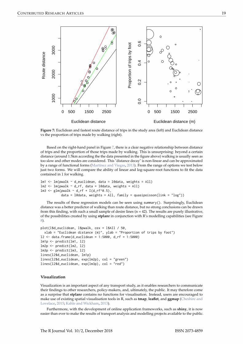
otFigure 7: Euclidean and fastest route distance of trips in the study area (left) and Euclidean distancevs the proportion of trips made by walking (right).

Based on the right-hand panel in Figure 7, there is a clear negative relationship between distanceof trips and the proportion of those trips made by walking. This is unsurprising: beyond a certaindistance (around 1.5km according the the data presented in the figure above) walking is usually seen astoo slow and other modes are considered. This "distance decay" is non-linear and can be approximatedby a range of functional forms (Martínez and Viegas, 2013). From the range of options we test belowjust two forms. We will compare the ability of linear and log-square-root functions to fit the datacontained in l for walking.

lm1 <- lm(pwalk ~ d_euclidean, data = l@data, weights = All)lm2 <- lm(pwalk ~ d_rf, data = l@data, weights = All)lm3 <- glm(pwalk ~ d_rf + I(d_rf^0.5),

data = l@data, weights = All, family = quasipoisson(link = "log"))

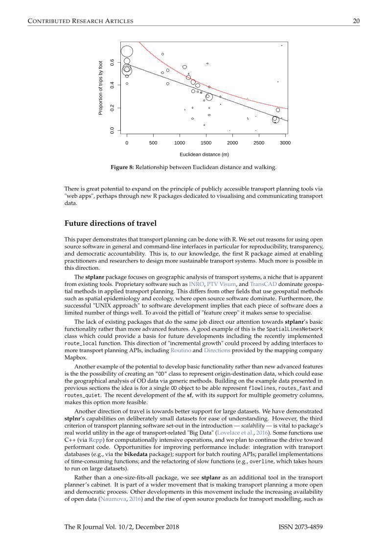
The results of these regression models can be seen using summary(). Surprisingly, Euclideandistance was a better predictor of walking than route distance, but no strong conclusions can be drawnfrom this finding, with such a small sample of desire lines (n = 42). The results are purely illustrative,of the possibilities created by using stplanr in conjunction with R’s modelling capabilities (see Figure8).

plot(l$d_euclidean, l$pwalk, cex = l$All / 50,xlab = "Euclidean distance (m)", ylab = "Proportion of trips by foot")

l2 <- data.frame(d_euclidean = 1:5000, d_rf = 1:5000)lm1p <- predict(lm1, l2)lm2p <- predict(lm2, l2)lm3p <- predict(lm3, l2)lines(l2$d_euclidean, lm1p)lines(l2$d_euclidean, exp(lm2p), col = "green")lines(l2$d_euclidean, exp(lm3p), col = "red")

Visualization

Visualization is an important aspect of any transport study, as it enables researchers to communicatetheir findings to other researchers, policy-makers, and, ultimately, the public. It may therefore comeas a surprise that stplanr contains no functions for visualisation. Instead, users are encouraged tomake use of existing spatial visualisation tools in R, such as tmap, leaflet, and ggmap (Cheshire andLovelace, 2015; Kahle and Wickham, 2013).

Furthermore, with the development of online application frameworks, such as shiny, it is noweasier than ever to make the results of transport analysis and modelling projects available to the public.

The R Journal Vol. 10/2, December 2018 ISSN 2073-4859

CONTRIBUTED RESEARCH ARTICLES 20

0 500 1000 1500 2000 2500 3000

0.0

0.2

0.4

0.6

Euclidean distance (m)

Pro

port

ion

of tr

ips

by fo

ot

Figure 8: Relationship between Euclidean distance and walking.

There is great potential to expand on the principle of publicly accessible transport planning tools via"web apps", perhaps through new R packages dedicated to visualising and communicating transportdata.

Future directions of travel

This paper demonstrates that transport planning can be done with R. We set out reasons for using opensource software in general and command-line interfaces in particular for reproducibility, transparency,and democratic accountability. This is, to our knowledge, the first R package aimed at enablingpractitioners and researchers to design more sustainable transport systems. Much more is possible inthis direction.

The stplanr package focuses on geographic analysis of transport systems, a niche that is apparentfrom existing tools. Proprietary software such as INRO, PTV Visum, and TransCAD dominate geospa-tial methods in applied transport planning. This differs from other fields that use geospatial methodssuch as spatial epidemiology and ecology, where open source software dominate. Furthermore, thesuccessful "UNIX approach" to software development implies that each piece of software does alimited number of things well. To avoid the pitfall of "feature creep" it makes sense to specialise.

The lack of existing packages that do the same job direct our attention towards stplanr’s basicfunctionality rather than more advanced features. A good example of this is the SpatialLinesNetworkclass which could provide a basis for future developments including the recently implementedroute_local function. This direction of "incremental growth" could proceed by adding interfaces tomore transport planning APIs, including Routino and Directions provided by the mapping companyMapbox.

Another example of the potential to develop basic functionality rather than new advanced featuresis the the possibility of creating an "OD" class to represent origin-destination data, which could easethe geographical analysis of OD data via generic methods. Building on the example data presented inprevious sections the idea is for a single OD object to be able represent flowlines, routes_fast androutes_quiet. The recent development of the sf, with its support for multiple geometry columns,makes this option more feasible.

Another direction of travel is towards better support for large datasets. We have demonstratedstplnr’s capabilities on deliberately small datasets for ease of understanding. However, the thirdcriterion of transport planning software set-out in the introduction — scalability — is vital to package’sreal world utility in the age of transport-related "Big Data" (Lovelace et al., 2016). Some functions useC++ (via Rcpp) for computationally intensive operations, and we plan to continue the drive towardperformant code. Opportunities for improving performance include: integration with transportdatabases (e.g., via the bikedata package); support for batch routing APIs; parallel implementationsof time-consuming functions; and the refactoring of slow functions (e.g., overline, which takes hoursto run on large datasets).

Rather than a one-size-fits-all package, we see stplanr as an additional tool in the transportplanner’s cabinet. It is part of a wider movement that is making transport planning a more openand democratic process. Other developments in this movement include the increasing availabilityof open data (Naumova, 2016) and the rise of open source products for transport modelling, such as

The R Journal Vol. 10/2, December 2018 ISSN 2073-4859

CONTRIBUTED RESEARCH ARTICLES 21

SUMO, MATSim, MITSIMLAB (Saidallah et al., 2016), and pgRouting. In this context, stplanr’s focuson GIS operations represents a niche in the market, allowing it to complement such software and helpmake better use of new open data sources. The stplanr package could also be used alongside other Rpackages that use spatial transport data such as aspace and MCI (Wieland, 2017).

The stplanr package was first developed to generate data for the Propensity to Cycle Tool (PCT),which estimates cycling potential down to the street level across all major cyclable routes in Englandand Wales (Lovelace et al., 2017). We believe there are many other national and international transportplanning challenges the package could be used to solve. In the context of the increasing availability ofopen access data6 packages for analyzing transport datasets. The stplanr package could help ensurethat the evidence on which transport planning decisions are based is reproducible, systematic, andtherefore democratically accountable.

Acknowledgements

We would like to thank a number of people and organisations who have supported the developmentof stplanr: the UK’s Department for Transport (DfT) for funding the Propensity to Cycle Tool (seewww.pct.bike), which instigated code which eventually became stplanr; Colin Gillespie, whoseteaching helped turn the code into a package; ROpenSci, for hosting the package (special thanksto Scott Chamberlin who reviewed the package); to Maëlle Salmon, Mark Padgham, Martin Lucas-Smith, and Marcus Young for commenting on early drafts of this paper; and to transport planningprofessionals Tom van Vuren (Mott MacDonald), John Parkin (University of the West of England),Helen Bowkett (Welsh Government), and Yaron Hollander, who provided input on the paper andideas for future priorities.

Bibliography

M. Balmer, M. Rieser, and K. Nagel. MATSim-T: Architecture and simulation times. Multi-agentsystems for traffic and transportation engineering, pages 57–78, 2009. URL https://svn.vsp.tu-berlin.de/repos/public-svn/publications/vspwp/2008/08-03/3aug08.pdf. [p7]

D. Banister. The sustainable mobility paradigm. Transport Policy, 15(2):73–80, 2008. URL https://doi.org/10.1016/j.tranpol.2007.10.005. [p7]

R. S. Bivand, E. J. Pebesma, and V. Gómez-Rubio. Applied spatial data analysis with R. Springer, NewYork, 2013. [p7, 8]

G. Boeing. OSMnx: New methods for acquiring, constructing, analyzing, and visualizing complexstreet networks. Computers, Environment and Urban Systems, 65:126–139, 2017. URL https://doi.org/10.1016/j.compenvurbsys.2017.05.004. [p21]

D. E. Boyce and H. C. W. L. Williams. Forecasting Urban Travel: Past, Present and Future. Edward ElgarPublishing, 2015. [p7]

P. E. Brown. Maps, Coordinate Reference Systems and Visualising Geographic Data with mapmisc.The R Journal, 8(1):64–91, 2016. URL https://journal.r-project.org/archive/2016/RJ-2016-005/index.html. [p7]

P. E. Brown and L. Zhou. diseasemapping: Modelling Spatial Variation in Disease Risk for Areal Data,2016. URL https://CRAN.R-project.org/package=diseasemapping. R package version 1.4.2. [p7]

F. Calabrese, G. Di Lorenzo, L. Liu, and C. Ratti. Estimating Origin-Destination Flows Using MobilePhone Location Data. IEEE Pervasive Computing, 10(4):36–44, 2011. URL https://doi.org/10.1109/MPRV.2011.41. [p11]

C. Calenge. The package adehabitat for the R software: tool for the analysis of space and habitat useby animals. Ecological Modelling, 197:1035, 2006. [p7]

E. Cerin, C. H. P. Sit, A. Barnett, M. C. Cheung, and W. M. Chan. Walking for recreation and perceptionsof the neighborhood environment in older Chinese urban dwellers. Journal of Urban Health, 90(1):56–66, 2013. URL https://doi.org/10.1007/s11524-012-9704-8. [p8]

6Two examples of this are the osmdata CRAN package (Padgham et al., 2017) and the Python package OSMnx(Boeing, 2017), for downloading and processing open access datasets from OpenStreetMap.

The R Journal Vol. 10/2, December 2018 ISSN 2073-4859

CONTRIBUTED RESEARCH ARTICLES 22

J. Cheshire and R. Lovelace. Spatial data visualisation with R. In C. Brunsdon and A. Singleton, editors,Geocomputation, pages 1–14. SAGE Publications, 2015. URL https://github.com/geocomPP/sdv.[p19]

CROW. Design manual for bicycle traffic. Kennisplatform, Amsterdam, 2007. URL http://www.crow.nl/publicaties/design-manual-for-bicycle-traffic. [p18]

R. Daniels and C. Mulley. Explaining walking distance to public transport: The dominance of publictransport supply. Journal of Transport and Land Use, 6(2):5, 2013. URL https://doi.org/10.5198/jtlu.v6i2.308. [p15]

M. Diana. Studying Patterns of Use of Transport Modes Through Data Mining. Transportation ResearchRecord: Journal of the Transportation Research Board, 2308:1–9, 2012. URL https://doi.org/10.3141/2308-01. [p8]

D. Efthymiou and C. Antoniou. Use of Social Media for Transport Data Collection. Procedia - Social andBehavioral Sciences, 48:775–785, 2012. URL http://dx.doi.org/10.1016/j.sbspro.2012.06.1055.[p8]

A. El-Geneidy, M. Grimsrud, R. Wasfi, P. Tétreault, and J. Surprenant-Legault. New evidence onwalking distances to transit stops: Identifying redundancies and gaps using variable service areas.Transportation, 41(1):193–210, 2014. URL https://doi.org/10.1007/s11116-013-9508-z. [p15]

Y. Hollander. Transport Modelling for a Complete Beginner. CTthink!, 2016. [p8]

M. Iacono, K. J. Krizek, and A. El-Geneidy. Measuring non-motorized accessibility: issues, alternatives,and execution. Journal of Transport Geography, 18(1):133–140, 2010. URL https://doi.org/10.1016/j.jtrangeo.2009.02.002. [p18]

H. Jalal, P. Pechlivanoglou, E. Krijkamp, F. Alarid-Escudero, E. Enns, and M. G. M. Hunink. AnOverview of R in Health Decision Sciences. Medical Decision Making, page 0272989X16686559. URLhttps://doi.org/10.1177/0272989X16686559. [p7]

D. Kahle and H. Wickham. ggmap: Spatial Visualization with ggplot2. The R Journal, 5(1):144–161,2013. URL https://journal.r-project.org/archive/2013/RJ-2013-014/index.html. [p19]

A. Y. Kim and J. Wakefield. SpatialEpi: Methods and Data for Spatial Epidemiology, 2016. URLhttps://CRAN.R-project.org/package=SpatialEpi. R package version 1.2.2. [p7]

D. Levinson and A. El-Geneidy. The minimum circuity frontier and the journey to work. RegionalScience and Urban Economics, 39(6):732–738, 2009. URL https://doi.org/10.1016/j.regsciurbeco.2009.07.003. [p17]

R. Lovelace, M. Birkin, P. Cross, and M. Clarke. From Big Noise to Big Data: Toward the Verification ofLarge Data sets for Understanding Regional Retail Flows. Geographical Analysis, 48(1):59–81, 2016.URL https://doi.org/10.1111/gean.12081. [p20]

R. Lovelace, A. Goodman, R. Aldred, N. Berkoff, A. Abbas, and J. Woodcock. The Propensity to CycleTool: An open source online system for sustainable transport planning. Journal of Transport and LandUse, 10(1), 2017. URL https://doi.org/10.5198/jtlu.2016.862. [p7, 8, 18, 21]

R. Lovelace, M. Morgan, L. Hama, and M. Padgham. Stats19: A package for working with open roadcrash data. Journal of Open Source Software, 2019. doi: 10.21105/joss.01181. [p9]

L. M. Martínez and J. M. Viegas. A new approach to modelling distance-decay functions for accessibilityassessment in transport studies. Journal of Transport Geography, 26:87–96, 2013. URL https://doi.org/10.1016/j.jtrangeo.2012.08.018. [p19]

R. D. D. Moore and D. Hutchinson. Why Watershed Analysts Should Use R for Data Processing andAnalysis. Confluence: Journal of Watershed Science and Management, 1(1). URL http://confluence-jwsm.ca/index.php/jwsm/article/view/2. [p7]

I. Naumova. Building Traffic Models Using Freely Available Data. PhD thesis, University of Hasselt, 2016.[p20]

J. d. D. Ortuzar and L. G. Willumsen. Modelling Transport. John Wiley & Sons, 2011. [p7, 8]

M. Padgham, R. Lovelace, M. Salmon, and B. Rudis. Osmdata. The Journal of Open Source Software, 2(14), 2017. URL https://doi.org/10.21105/joss.00305. [p21]

The R Journal Vol. 10/2, December 2018 ISSN 2073-4859

CONTRIBUTED RESEARCH ARTICLES 23

E. Pebesma, R. Bivand, and P. Ribeiro. Software for spatial statistics. Journal of Statistical Software,Articles, 63(1):1–8, 2015. ISSN 1548-7660. URL https://doi.org/10.18637/jss.v063.i01. [p8]

M. Saidallah, A. El Fergougui, and A. E. Elalaoui. A comparative study of urban road traffic simulators.MATEC Web Conf., 81:05002, 2016. URL https://doi.org/10.1051/matecconf/20168105002. [p21]

F. Simini, M. C. González, A. Maritan, and A.-L. Barabási. A universal model for mobility andmigration patterns. Nature, pages 8–12, 2012. URL https://doi.org/10.1038/nature10856. [p18]

P. Waddell. UrbanSim: Modeling urban development for land use, transportation, and environmentalplanning. Journal of the American Planning Association, 68(3):297–314, 2002. [p8]

K. Walker. tigris: An R Package to Access and Work with Geographic Data from the US Census Bureau.The R Journal, 8(2):231–242, 2016. URL https://journal.r-project.org/archive/2016/RJ-2016-043/index.html. [p9]

T. Wieland. Market Area Analysis for Retail and Service Locations with MCI. The R Journal, 9(1):298–323, 2017. URL https://journal.r-project.org/archive/2017/RJ-2017-020/index.html.[p21]

X. Zheng, W. Chen, P. Wang, D. Shen, S. Chen, X. Wang, Q. Zhang, and L. Yang. Big data for socialtransportation. IEEE Transactions on Intelligent Transportation Systems, 17(3):620–630, 2016. URLhttp://ieeexplore.ieee.org/abstract/document/7359138/. [p7]

Robin LovelaceUniversity of LeedsLeeds Institute for Transport StudiesLeeds Institute for Data Analytics34-40 University RoadLS2 9JT, UKr.lovelace@leeds.ac.uk

Richard EllisonUniversity of Sydney378 Abercrombie StreetDarlington, NSW 2008, Australiarichard.ellison@sydney.edu.au

The R Journal Vol. 10/2, December 2018 ISSN 2073-4859