storage size determination for grid-connected photovoltaic
TRANSCRIPT

arX
iv:1
109.
4102
v2 [
mat
h.O
C]
10 J
an 2
012
1
Storage Size Determination for Grid-ConnectedPhotovoltaic Systems
Yu Ru, Jan Kleissl, and Sonia Martinez
Abstract—In this paper, we study the problem of determiningthe size of battery storage used in grid-connected photovoltaic(PV) systems. In our setting, electricity is generated fromPVand is used to supply the demand from loads. Excess electricitygenerated from the PV can be stored in a battery to be used lateron, and electricity must be purchased from the electric gridif thePV generation and battery discharging cannot meet the demand.Due to the time-of-use electricity pricing, electricity can also bepurchased from the grid when the price is low, and be sold backto the grid when the price is high. The objective is to minimizethe cost associated with purchasing from (or selling back to) theelectric grid and the battery capacity loss while at the sametimesatisfying the load and reducing the peak electricity purchasefrom the grid. Essentially, the objective function dependson thechosen battery size. We want to find a unique critical value(denoted asCc
ref) of the battery size such that the total costremains the same if the battery size is larger than or equal toCc
ref , and the cost is strictly larger if the battery size is smallerthan Cc
ref . We obtain a criterion for evaluating the economicvalue of batteries compared to purchasing electricity fromthegrid, propose lower and upper bounds onCc
ref , and introducean efficient algorithm for calculating its value; these results arevalidated via simulations.
I. I NTRODUCTION
The need to reduce greenhouse gas emissions due to fossilfuels and the liberalization of the electricity market haveledto large scale development of renewable energy generatorsin electric grids [1]. Among renewable energy technologiessuch as hydroelectric, photovoltaic (PV), wind, geothermal,biomass, and tidal systems, grid-connected solar PV continuedto be the fastest growing power generation technology, witha 70% increase in existing capacity to13GW in 2008 [2].However, solar energy generation tends to be variable due tothe diurnal cycle of the solar geometry and clouds. Storagedevices (such as batteries, ultracapacitors, compressed air, andpumped hydro storage [3]) can be used to i) smooth out thefluctuation of the PV output fed into electric grids (“capacityfirming”) [2], [4], ii) discharge and augment the PV outputduring times of peak energy usage (“peak shaving”) [5], oriii) store energy for nighttime use, for example in zero-energybuildings and residential homes.
Depending on the specific application (whether it is off-grid or grid-connected), battery storage size is determinedbased on the battery specifications such as the battery storagecapacity (and the minimum battery charging/discharging time).For off-grid applications, batteries have to fulfill the followingrequirements: (i) the discharging rate has to be larger than
Yu Ru, Jan Kleissl, and Sonia Martinez are with the Mechani-cal and Aerospace Engineering Department, University of California,San Diego (e-mail:[email protected], [email protected],[email protected]).
or equal to the peak load capacity; (ii) the battery storagecapacity has to be large enough to supply the largest night timeenergy use and to be able to supply energy during the longestcloudy period (autonomy). The IEEE standard [6] providessizing recommendations for lead-acid batteries in stand-alonePV systems. In [7], the solar panel size and the battery sizehave been selected via simulations to optimize the operation ofa stand-alone PV system, which considers reliability measuresin terms of loss of load hours, the energy loss and thetotal cost. In contrast, if the PV system is grid-connected,autonomy is a secondary goal; instead, batteries can reducethe fluctuation of PV output or provide economic benefits suchas demand charge reduction, and arbitrage. The work in [8]analyzes the relation between available battery capacity andoutput smoothing, and estimates the required battery capacityusing simulations. In addition, the battery sizing problemhasbeen studied for wind power applications [9]–[11] and hybridwind/solar power applications [12]–[14]. In [9], design ofabattery energy storage system is examined for the purposeof attenuating the effects of unsteady input power from windfarms, and solution to the problem via a computational proce-dure results in the determination of the battery energy storagesystem’s capacity. Similarly, in [11], based on the statistics oflong-term wind speed data captured at the farm, a dispatchstrategy is proposed which allows the battery capacity to bedetermined so as to maximize a defined service lifetime/unitcost index of the energy storage system; then a numericalapproach is used due to the lack of an explicit mathematicalexpression to describe the lifetime as a function of the batterycapacity. In [10], sizing and control methodologies for azinc-bromine flow battery-based energy storage system areproposed to minimize the cost of the energy storage system.However, the sizing of the battery is significantly impactedbyspecific control strategies. In [12], a methodology for calcu-lating the optimum size of a battery bank and the PV arrayfor a stand-alone hybrid wind/PV system is developed, and asimulation model is used to examine different combinationsof the number of PV modules and the number of batteries.In [13], an approach is proposed to help designers determinethe optimal design of a hybrid wind-solar power system;the proposed analysis employs linear programming techniquesto minimize the average production cost of electricity whilemeeting the load requirements in a reliable manner. In [14],genetic algorithms are used to optimally size the hybrid systemcomponents, i.e., to select the optimal wind turbine and PVrated power, battery energy storage system nominal capacityand inverter rating. The primary optimization objective istheminimization of the levelized energy cost of the island systemover the entire lifetime of the project.

2
In this paper, we study the problem of determining thebattery size for grid-connected PV systems. The targetedapplications are primarily electricity customers with PV arrays“behind the meter,” such as residential and commercial build-ings with rooftop PVs. In such applications, the objective is toreduce the energy cost and the loss of investment on storagedevices due to aging effects while satisfying the loads andreducing peak electricity purchase from the grid (instead ofsmoothing out the fluctuation of the PV output fed into electricgrids). Our setting1 is shown in Fig. 1. Electricity is generatedfrom PV panels, and is used to supply different types ofloads. Battery storage is used to either store excess electricitygenerated from PV systems for later use when PV generationis insufficient to serve the load, or purchase electricity from thegrid when the time-of-use pricing is lower and sell back to thegrid when the time-of-use pricing is higher. Without a battery,if the load was too large to be supplied by PV generatedelectricity, electricity would have to be purchased from thegrid to meet the demand. Naturally, given the high cost ofbattery storage, the size of the battery storage should be chosensuch that the cost of electricity purchase from the grid and theloss of investment on batteries are minimized. Intuitively, ifthe battery is too large, the electricity purchase cost could bethe same as the case with a relatively smaller battery. In thispaper, we show that there is a unique critical value (denotedasCc
ref, refer to Problem 1) of the battery capacity such thatthe cost of electricity purchase and the loss of investmentsonbatteries remains the same if the battery size is larger thanorequal toCc
ref and the cost is strictly larger if the battery sizeis smaller thanCc
ref. We obtain a criterion for evaluating theeconomic value of batteries compared to purchasing electricityfrom the grid, propose lower and upper bounds onCc
ref giventhe PV generation, loads, and the time period for minimizingthe costs, and introduce an efficient algorithm for calculatingthe critical battery capacity based on the bounds; these resultsare validated via simulations.
The contributions of this work are the following: i) to thebest of our knowledge, this is the first attempt on determiningthe battery size for grid-connected PV systems based on atheoretical analysis on the lower and upper bounds of thebattery size; in contrast, most previous work are based onsimulations, e.g., the work in [8]–[12]; ii) a criterion foreval-uating the economic value of batteries compared to purchasingelectricity from the grid is derived (refer to Proposition 4andAssumption 2), which can be easily calculated and could bepotentially used for choosing appropriate battery technologiesfor practical applications; and iii) lower and upper boundsonthe battery size are proposed, and an efficient algorithm isintroduced to calculate its value for the given PV generationand dynamic loads; these results are then validated using sim-ulations. Simulation results illustrate the benefits of employingbatteries in grid-connected PV systems via peak shaving andcost reductions compared with the case without batteries (thisis discussed in Section V.B).
1Note that solar panels and batteries both operate on DC, while the grid andloads operate on AC. Therefore, DC-to-AC and AC-to-DC powerconversionis necessary when connecting solar panels and batteries with the grid andloads.
The paper is organized as follows. In the next section, we layout our setting, and formulate the storage size determinationproblem. Lower and upper bounds onCc
ref are proposedin Section III. Algorithms are introduced in Section IV tocalculate the value of the critical battery capacity. In Section V,we validate the results via simulations. Finally, conclusionsand future directions are given in Section VI.
II. PROBLEM FORMULATION
In this section, we formulate the problem of determiningthe storage size for a grid-connected PV system, as shown inFig. 1. We first introduce different components in our setting.
A. Photovoltaic Generation
We use the following equation to calculate the electricitygenerated from solar panels:
Ppv(t) = GHI(t)× S × η , (1)
where• GHI (Wm−2) is the global horizontal irradiation at the
location of solar panels,• S (m2) is the total area of solar panels, and• η is the solar conversion efficiency of the PV cells.
The PV generation model is a simplified version of the oneused in [15] and does not account for PV panel temperatureeffects.2
B. Electric Grid
Electricity can be purchased from or sold back to the grid.For simplicity, we assume that the prices for sales and pur-chases at timet are identical and are denoted asCg(t)($/Wh).Time-of-use pricing is used (Cg(t) ≥ 0 depends ont) becausecommercial buildings with PV systems that would considera battery system usually pay time-of-use electricity rates.In addition, with increased deployment of smart meters andelectric vehicles, some utility companies are moving towardsresidential time-of-use pricing as well; for example, SDG&E
2Note that our analysis on determining battery capacity onlyrelies onPpv(t) instead of detailed models of the PV generation. Therefore,morecomplicated PV generation models can also be incorporated into the costminimization problem as discussed in Section II.F.
Solar Panel
Electric Grid Battery
Load
DC/AC
DC
/AC
AC
/DC
AC Bus
Fig. 1. Grid-connected PV system with battery storage and loads.

3
(San Diego Gas & Electric) has the peak, semipeak, offpeakprices for a day in the summer season [16], as shown in Fig. 3.
We usePg(t)(W ) to denote the electric power exchangedwith the grid with the interpretation that
• Pg(t) > 0 if electric power is purchased from the grid,• Pg(t) < 0 if electric power is sold back to the grid.
In this way, positive costs are associated with the electricitypurchase from the grid, and negative costs with the electricitysold back to the grid. In this paper, peak shaving is enforcedthrough the constraint that
Pg(t) ≤ D ,
whereD is a positive constant.
C. Battery
A battery has the following dynamic:
dEB(t)
dt= PB(t) , (2)
whereEB(t)(Wh) is the amount of electricity stored in thebattery at timet, andPB(t)(W ) is the charging/dischargingrate; more specifically,
• PB(t) > 0 if the battery is charging,• andPB(t) < 0 if the battery is discharging.
For certain types of batteries, higher order models exist (e.g.,a third order model is proposed in [17], [18]).
To take into account battery aging, we useC(t)(Wh) to de-note the usable battery capacity at timet. At the initial timet0,the usable battery capacity isCref, i.e.,C(t0) = Cref ≥ 0. Thecumulative capacity loss at timet is denoted as∆C(t)(Wh),and∆C(t0) = 0. Therefore,
C(t) = Cref −∆C(t) .
The battery aging satisfies the following dynamic equation
d∆C(t)
dt=
{
−ZPB(t) if PB(t) < 0
0 otherwise ,(3)
whereZ > 0 is a constant depending on battery technologies.This aging model is derived from the aging model in [5]under certain reasonable assumptions; the detailed derivationis provided in the Appendix. Note that there is a capacity lossonly when electricity is discharged from the battery. Therefore,∆C(t) is a nonnegative and non-decreasing function oft.
We consider the following constraints on the battery:i) At any time, the battery chargeEB(t) should satisfy
0 ≤ EB(t) ≤ C(t) = Cref −∆C(t) ,
ii) The battery charging/discharging rate should satisfy
PBmin ≤ PB(t) ≤ PBmax ,
where PBmin < 0, −PBmin is the maximum batterydischarging rate, andPBmax > 0 is the maximum batterycharging rate. For simplicity, we assume that
PBmax = −PBmin =C(t)
Tc
=Cref −∆C(t)
Tc
,
where constantTc > 0 is the minimum time required tocharge the battery from0 to C(t) or discharge the batteryfrom C(t) to 0.
D. Load
Pload(t)(W ) denotes the load at timet. We do not makeexplicit assumptions on the load considered in Section IIIexcept thatPload(t) is a (piecewise) continuous function. Inresidential home settings, loads could have a fixed schedulesuch as lights and TVs, or a relatively flexible schedulesuch as refrigerators and air conditioners. For example, airconditioners can be turned on and off with different schedulesas long as the room temperature is within a comfortable range.
E. Converters for PV and Battery
Note that the PV, battery, grid, and loads are all connectedto an AC bus. Since PV generation is operated on DC, a DC-to-AC converter is necessary, and its efficiency is assumed tobe a constantηpv satisfying
0 < ηpv ≤ 1 .
Since the battery is also operated on DC, an AC-to-DCconverter is necessary when charging the battery, and a DC-to-AC converter is necessary when discharging as shown inFig. 1. For simplicity, we assume that both converters havethe same constant conversion efficiencyηB satisfying
0 < ηB ≤ 1 .
We define
PBC(t) =
{
ηBPB(t) if PB(t) < 0PB(t)ηB
otherwise ,
In other words,PBC(t) is the power exchanged with the ACbus when the converters and the battery are treated as an entity.Similarly, we can derive
PB(t) =
{
PBC(t)ηB
if PBC(t) < 0
ηBPBC(t) otherwise ,
Note thatη2B is the round trip efficiency of the battery storage.
F. Cost Minimization
With all the components introduced earlier, now we canformulate the following problem of minimizing the sum ofthe net power purchase cost3 and the cost associated with thebattery capacity loss while guaranteeing that the demand from
3Note that the net power purchase cost include the positive cost to purchaseelectricity from the grid, and the negative cost to sell electricity back to thegrid.

4
loads and the peak shaving requirement are satisfied:
minPB ,Pg
∫ t0+T
t0
Cg(τ)Pg(τ)dτ +K∆C(t0 + T )
s.t. ηpvPpv(t) + Pg(t) = PBC(t) + Pload(t) , (6)
dEB(t)
dt= PB(t) ,
d∆C(t)
dt=
{
−ZPB(t) if PB(t) < 0
0 otherwise ,
0 ≤ EB(t) ≤ Cref −∆C(t) ,
EB(t0) = 0 ,∆C(t0) = 0 ,
PBmin ≤ PB(t) ≤ PBmax ,
PBmax = −PBmin =Cref −∆C(t)
Tc
,
PB(t) =
{
PBC(t)ηB
if PBC(t) < 0
ηBPBC(t) otherwise ,
Pg(t) ≤ D , (7)
wheret0 is the initial time,T is the time period consideredfor the cost minimization,K($/Wh) > 0 is the unit cost forthe battery capacity loss. Note that:
i) No cost is associated with PV generation. In other words,PV generated electricity is assumed free;
ii) K∆C(t0 + T ) is the loss of the battery purchase invest-ment during the time period fromt0 to t0+T due to theuse of the battery to reduce the net power purchase cost;
iii) Eq. (6) is the power balance requirement for any timet ∈ [t0, t0 + T ];
iv) the constraintPg(t) ≤ D captures the peak shavingrequirement.
Given a battery of initial capacityCref, on the one hand, ifthe battery is rarely used, then the cost due to the capacityloss K∆C(t0 + T ) is low while the net power purchasecost
∫ t0+T
t0Cg(τ)Pg(τ)dτ is high; on the other hand, if the
battery is used very often, then the net power purchase cost∫ t0+T
t0Cg(τ)Pg(τ)dτ is low while the cost due to the capacity
lossK∆C(t0 + T ) is high. Therefore, there is a tradeoff onthe use of the battery, which is characterized by calculatingan optimal control policy onPB(t), Pg(t) to the optimizationproblem in Eq. (7).
Remark 1 Besides the constraintPg(t) ≤ D, peak shaving isalso accomplished indirectly through dynamic pricing. Time-of-use price margins and schedules are motivated by thepeak load magnitude and timing. Minimizing the net powerpurchase cost results in battery discharge and reduction ingridpurchase during peak times. If, however, the peak load for acustomer falls into the off-peak time period, then the constraintonPg(t) limits the amount of electricity that can be purchased.Peak shaving capabilities of the constraintPg(t) ≤ D anddynamic pricing will be illustrated in Section V.B. �
G. Storage Size Determination
Based on Eq. (6), we obtain
Pg(t) = Pload(t)− ηpvPpv(t) + PBC(t) .
Let u(t) = PBC(t), then the optimization problem in Eq. (7)can be rewritten as
minu
∫ t0+T
t0Cg(τ)(Pload(τ) − ηpvPpv(τ) + u(τ))dτ +K∆C(t0 + T )
s.t.dEB(t)
dt=
{
u(t)ηB
if u(t) < 0
ηBu(t) otherwise ,
d∆C(t)
dt=
{
−Z u(t)ηB
if u(t) < 0
0 otherwise ,
EB(t) ≥ 0 , EB(t0) = 0 ,∆C(t0) = 0 ,
EB(t) + ∆C(t) ≤ Cref ,
ηBu(t)Tc +∆C(t) ≤ Cref if u(t) > 0,
−u(t)
ηBTc +∆C(t) ≤ Cref if u(t) < 0,
Pload(t)− ηpvPpv(t) + u(t) ≤ D . (8)
Now it is clear that onlyu(t) is an independent variable. Wedefine the set of feasible controls as controls that guaranteeall the constraints in the optimization problem in Eq. (8).
Let J denote the objective function
minu∫ t0+T
t0Cg(τ)(Pload(τ) − ηpvPpv(τ) + u(τ))dτ +K∆C(t0 + T ) .
If we fix the parameterst0, T,K, Z, Tc, andD, J is a functionof Cref, which is denoted asJ(Cref). If we increaseCref,intuitively J will decrease though may not strictly decrease(this is formally proved in Proposition 2) because the batterycan be utilized to decrease the cost by
i) storing extra electricity generated from PV or purchasingelectricity from the grid when the time-of-use pricing islow, and
ii) supplying the load or selling back when the time-of-usepricing is high.
Now we formulate the following storage size determinationproblem.
Problem 1 (Storage Size Determination) Given the opti-mization problem in Eq. (8) with fixedt0, T,K, Z, Tc, andD, determine a critical valueCc
ref ≥ 0 such that
• ∀Cref < Ccref, J(Cref) > J(Cc
ref), and• ∀Cref ≥ Cc
ref, J(Cref) = J(Ccref).
One approach to calculate the critical valueCcref is that we
first obtain an explicit expression for the functionJ(Cref) bysolving the optimization problem in Eq. (8) and then solvefor Cc
ref based on the functionJ . However, the optimizationproblem in Eq. (8) is difficult to solve due to the nonlinearconstraints onu(t) andEB(t), and the fact that it is hard toobtain analytical expressions forPload(t) andPpv(t) in reality.Even though it might be possible to find the optimal controlusing the minimum principle [19], it is still hard to get anexplicit expression for the cost functionJ . Instead, in the nextsection, we identify conditions under which the storage sizedetermination problem results in non-trivial solutions (namely,Cc
ref is positive and finite), and then propose lower and upperbounds on the critical battery capacityCc
ref.

5
III. B OUNDS ONCcref
Now we examine the cost minimization problem in Eq. (8).SincePload(t)− ηpvPpv(t)+u(t) ≤ D, or equivalently,u(t) ≤D+ηpvPpv(t)−Pload(t), is a constraint that has to be satisfiedfor any t ∈ [t0, t0 + T ], there are scenarios in which eitherthere is no feasible control oru(t) = 0 for t ∈ [t0, t0 + T ].GivenPpv(t), Pload(t), andD, we define
S1 = {t ∈ [t0, t0 + T ] | D + ηpvPpv(t)− Pload(t) < 0} , (9)
S2 = {t ∈ [t0, t0 + T ] | D + ηpvPpv(t)− Pload(t) = 0} , (10)
S3 = {t ∈ [t0, t0 + T ] | D + ηpvPpv(t)− Pload(t) > 0} . (11)
Note that4 S1⊕S2⊕S3 = [t0, t0+T ]. Intuitively, S1 is the setof time instants at which the battery can only be discharged,S2 is the set of time instants at which the battery can bedischarged or is not used (i.e.,u(t) = 0), andS3 is the set oftime instants at which the battery can be charged, discharged,or is not used.
Proposition 1 Given the optimization problem in Eq. (8), if
i) t0 ∈ S1, orii) S3 is empty, oriii) t0 /∈ S1 (or equivalently,t0 ∈ S2 ∪ S3), S3 is nonempty,
S1 is nonempty, and∃t1 ∈ S1, ∀t3 ∈ S3, t1 < t3,
then either there is no feasible control oru(t) = 0 for t ∈[t0, t0 + T ].
Proof: Now we prove that, under these three cases, eitherthere is no feasible control oru(t) = 0 for t ∈ [t0, t0 + T ].
i) If t0 ∈ S1, thenu(t0) ≤ D+ ηpvPpv(t0)− Pload(t0) < 0.However, sinceEB(t0) = 0, the battery cannot bedischarged at timet0. Therefore, there is no feasiblecontrol.
ii) If S3 is empty, it means thatu(t0) ≤ D + ηpvPpv(t0) −Pload(t0) ≤ 0 for any t ∈ [t0, t0 + T ], which implies thatthe battery can never be charged. IfS1 is nonempty, thenthere exists some time instant when the battery has to bedischarged. SinceEB(t0) = 0 and the battery can neverbe charged, there is no feasible control. IfS1 is empty,thenu(t) = 0 for any t ∈ [t0, t0 +T ] is the only feasiblecontrol becauseEB(t0) = 0.
iii) In this case, the battery has to be discharged at timet1,but the charging can only happen at time instantt3 ∈ S3.If ∀t3 ∈ S3, ∃t1 ∈ S1 such thatt1 < t3, then the batteryis always discharged before possibly being charged. SinceEB(t0) = 0, then there is no feasible control.
Note that if the only feasible control isu(t) = 0 for t ∈[t0, t0+T ], then the battery is not used. Therefore, we imposethe following assumption.
Assumption 1 In the optimization problem in Eq. (8),t0 ∈S2 ∪ S3, S3 is nonempty, and either
• S1 is empty, or• S1 is nonempty, but∀t1 ∈ S1, ∃t3 ∈ S3, t3 < t1,
whereS1, S2, S3 are defined in Eqs. (9), (10), (11).
4C = A⊕ B meansC = A ∪ B andA ∩ B = ∅.
Given Assumption 1, there exists at least one feasiblecontrol. Now we examine howJ(Cref) changes whenCref
increases.
Proposition 2 Consider the optimization problem in Eq. (8)with fixed t0, T,K, Z, Tc, and D. If C1
ref < C2ref, then
J(C1ref) ≥ J(C2
ref).
Proof: Given C1ref, suppose controlu1(t) achieves the
minimum costJ(C1ref) and the corresponding states for the
battery charge and capacity loss areE1B(t) and∆C1(t). Since
E1B(t) + ∆C1(t) ≤ C1
ref < C2ref ,
ηBu1(t)Tc +∆C1(t) ≤ C1
ref < C2ref if u
1(t) > 0,
−u1(t)
ηBTc +∆C1(t) ≤ C1
ref < C2ref if u
1(t) < 0,
Pload(t)− ηpvPpv(t) + u1(t) ≤ D ,
u1(t) is also a feasible control for problem (8) withC2ref, and
results in the costJ(C1ref). SinceJ(C2
ref) is the minimum costover the set of all feasible controls which includeu1(t), wemust haveJ(C1
ref) ≥ J(C2ref).
In other words,J is non-increasing with respect to theparameterCref, i.e., J is monotonically decreasing (thoughmay not be strictly monotonically decreasing). IfCref = 0,then0 ≤ ∆C(t) ≤ Cref = 0, which implies thatu(t) = 0. Inthis case,J has the largest value
Jmax = J(0) =
∫ t0+T
t0
Cg(τ)(Pload(τ)−ηpvPpv(τ))dτ . (12)
Proposition 2 also justifies the storage size determinationproblem. Note that the critical valueCc
ref (as defined inProblem 1) is unique as shown below.
Proposition 3 Given the optimization problem in Eq. (8) withfixed t0, T,K, Z, Tc, andD, Cc
ref is unique.
Proof: We prove it via contradiction. SupposeCcref is not
unique. In other words, there are two different critical valuesCc1
ref andCc2ref. Without loss of generality, supposeCc1
ref < Cc2ref.
By definition, J(Cc1ref) > J(Cc2
ref) becauseCc2ref is a critical
value, whileJ(Cc1ref) = J(Cc2
ref) becauseCc1ref is a critical value.
A contradiction. Therefore, we must haveCc1ref = Cc2
ref.Intuitively, if the unit cost for the battery capacity lossK is
higher (compared with purchasing electricity from the grid),then it might be preferable that the battery is not used at all,which results inCc
ref = 0, as shown below.
Proposition 4 Consider the optimization problem in Eq. (8)with fixed t0, T,K, Z, Tc, andD under Assumption 1.
i) If
K ≥(maxt Cg(t)−mint Cg(t))ηB
Z,
thenJ(Cref) = Jmax, which implies thatCcref = 0;
ii) if
K <(maxt Cg(t)−mint Cg(t))ηB
Z,

6
then
J(Cref) ≥Jmax− (maxt
Cg(t)−mint
Cg(t)−KZ
ηB)×
T × (D +maxt
(ηpvPpv(t)− Pload(t))) ,
wheremaxt andmint are calculated fort ∈ [t0, t0 + T ].
Proof: The cost function can be rewritten as
J(Cref) =Jmax+
∫ t0+T
t0
Cg(τ)u(τ)dτ +K∆C(t0 + T )
=Jmax+
∫ t0+T
t0
Cg(τ)u(τ)dτ+
K
∫ t0+T
t0
−Zu(τ)
ηB|u(τ)<0dτ
=Jmax+ J+ + J− ,
where
J+ =
∫ t0+T
t0
Cg(τ)u(τ)|u(τ)>0dτ ,
and
J− =
∫ t0+T
t0
(Cg(τ)−KZ
ηB)u(τ)|u(τ)<0dτ .
Note thatJ+ ≥ 0 because the integrandCg(τ)u(τ)|u(τ)>0 isalways nonnegative.
i) We first considerK ≥(maxt Cg(t)−mint Cg(t))ηB
Z. There
are two possibilities:
• K ≥(maxt Cg(t))ηB
Z, or equivalently,maxt Cg(t) ≤
KZηB
.Thus, for anyt ∈ [t0, t0 + T ], Cg(t) −
KZηB
≤ 0, whichimplies thatJ− ≥ 0. Therefore,J(Cref) ≥ Jmax.
•(maxt Cg(t)−mint Cg(t))ηB
Z≤ K <
(maxt Cg(t))ηB
Z.
Let A1 = maxt Cg(t) − KZηB
, then A1 > 0.Let A2 = mint Cg(t), then A2 ≥ 0. Since(maxt Cg(t)−mint Cg(t))ηB
Z≤ K, A2 ≥ A1. Now we
have J+ ≥ A2
∫ t0+T
t0u(τ)|u(τ)>0dτ , and J− ≥
A1
∫ t0+T
t0u(τ)|u(τ)<0dτ . Therefore,
J(Cref) ≥Jmax+A2
∫ t0+T
t0
u(τ)|u(τ)>0dτ+
A1
∫ t0+T
t0
u(τ)|u(τ)<0dτ
=Jmax+ (A2 − A1)
∫ t0+T
t0
u(τ)|u(τ)>0dτ+
A1
∫ t0+T
t0
u(τ)dτ
≥Jmax+A1
∫ t0+T
t0
u(τ)dτ .
SinceEB(t0 + T ) = EB(t0) +∫ t0+T
t0PB(τ)dτ ≥ 0 and
EB(t0) = 0, we have
0 ≤
∫ t0+T
t0
PB(τ)dτ
=
∫ t0+T
t0
PB(τ)|PB(τ)>0dτ +
∫ t0+T
t0
PB(τ)|PB (τ)<0dτ
=
∫ t0+T
t0
u(τ)ηB|u(τ)>0dτ +
∫ t0+T
t0
u(τ)
ηB|u(τ)<0dτ
≤
∫ t0+T
t0
u(τ)|u(τ)>0dτ +
∫ t0+T
t0
u(τ)|u(τ)<0dτ
=
∫ t0+T
t0
u(τ)dτ . (13)
Therefore, we haveJ(Cref) ≥ Jmax.
In summary, if K ≥(maxt Cg(t)−mint Cg(t))ηB
Z, we have
J(Cref) ≥ Jmax, which implies thatJ(Cref) ≥ J(0). SinceJ(Cref) is a non-increasing function ofCref, we also haveJ(Cref) ≤ J(0). Therefore, we must haveJ(Cref) = J(0) =Jmax for Cref ≥ 0, andCc
ref = 0 by definition.ii) We now considerK <
(maxt Cg(t)−mint Cg(t))ηB
Z, which
implies thatA1 > A2 ≥ 0. Then
J(Cref) ≥Jmax+A2
∫ t0+T
t0
u(τ)|u(τ)>0dτ+
A1
∫ t0+T
t0
u(τ)|u(τ)<0dτ
=Jmax+A2
∫ t0+T
t0
u(τ)dτ+
(A1 −A2)
∫ t0+T
t0
u(τ)|u(τ)<0dτ .
Since∫ t0+T
t0u(τ)dτ ≥ 0 as argued in the proof toi),
J(Cref) ≥ Jmax + (A1 − A2)∫ t0+T
t0u(τ)|u(τ)<0dτ . Now
we try to lower bound∫ t0+T
t0u(τ)|u(τ)<0dτ . Note that
∫ t0+T
t0u(τ)dτ ≥ 0 (as shown in Eq. (13)) implies that
∫ t0+T
t0
u(τ)|u(τ)<0dτ ≥ −
∫ t0+T
t0
u(τ)|u(τ)>0dτ .
Given Assumption 1,S3 is nonempty, which implies thatD + maxt(ηpvPpv(t) − Pload(t)) > 0. Since u(t) ≤ D +ηpvPpv(t) − Pload(t) ≤ D + maxt(ηpvPpv(t) − Pload(t)),∫ t0+T
t0u(τ)|u(τ)>0dτ ≤ T×(D+maxt(ηpvPpv(t)−Pload(t))),
which implies that
∫ t0+T
t0u(τ)|u(τ)<0dτ ≥ −T × (D +maxt(ηpvPpv(t)− Pload(t))) . (14)
In summary,J(Cref) ≥ Jmax − (A1 − A2) × T × (D +maxt(ηpvPpv(t)− Pload(t))), which proves the result.
Remark 2 Note thati) in Proposition 4 provides a criterionfor evaluating the economic value of batteries compared topurchasing electricity from the grid. In other words, only ifthe unit cost of the battery capacity loss satisfies
K <(maxt Cg(t)−mint Cg(t))ηB
Z,

7
it is desirable to use battery storages. This criterion depends onthe pricing signal (especially the difference between the max-imum and the minimum of the pricing signal), the conversionefficiency of the battery converters, and the aging coefficientZ. �
Given the result in Proposition 4, we impose the followingadditional assumption on the unit cost of the battery capacityloss to guarantee thatCc
ref is positive.
Assumption 2 In the optimization problem in Eq. (8),
K <(maxt Cg(t)−mint Cg(t))ηB
Z.
In other words, the cost of the battery capacity loss duringoperations is less than the potential gain expressed as themargin between peak and off-peak prices modified by theconversion efficiency of the battery converters and the batteryaging coefficient. SinceJ(Cref) is a non-increasing function ofCref and lower bounded by a finite value given Assumptions 1and 2, the storage size determination problem is well defined.Now we show lower and upper bounds on the critical batterycapacity in the following proposition.
Proposition 5 Consider the optimization problem in Eq. (8)with fixed t0, T,K, Z, Tc, andD under Assumptions 1 and 2.ThenC lb
ref ≤ Ccref ≤ Cub
ref, where
C lbref = max(
Tc
ηB× (max
t(Pload(t)− ηpvPpv(t))−D), 0) ,
and
Cubref = max(ηBTc+
ZT
ηB, ηBT )×(D+max
t(ηpvPpv(t)−Pload(t)) .
Proof: We first show the lower bound via contradic-tion. Without loss of generality, we assume thatTc
ηB×
(maxt(Pload(t) − ηpvPpv(t)) − D) > 0 (because we requireCc
ref ≥ 0). Suppose
Ccref < C lb
ref =Tc
ηB× (max
t(Pload(t)− ηpvPpv(t)) −D) ,
or equivalently,
D < −Cc
refηB
Tc
+maxt
(Pload(t)− ηpvPpv(t)) .
Therefore, there existst1 ∈ [t0, t0 + T ] such thatD <
−Cc
refηB
Tc+Pload(t1)−ηpvPpv(t1). Sinceu(t1) ≤ D−Pload(t1)+
ηpvPpv(t1) < −Cc
refηB
Tc≤ 0, we have
PB(t1) =u(t1)
ηB≤
D + ηpvPpv(t1)− Pload(t1)
ηB
< −Cc
ref
Tc
≤ −Cref −∆C(t1)
Tc
= PBmin .
The implication is that the control does not satisfy the dis-charging constraint att1. Therefore,C lb
ref ≤ Ccref.
To showCcref ≤ Cub
ref, it is sufficient to show that ifCref ≥Cub
ref, the electricity that can be stored never exceedsCubref.
Note that the battery charging is limited byPBmax, i.e.,PB(t) = ηBu(t) ≤ PBmax. Now we try to lower boundPBmax.
PBmax =Cref −∆C(t)
Tc
≥Cref −∆C(t0 + T )
Tc
,
in which the second inequality holds because∆C(t) is anon-decreasing function oft. By applying the aging modelin Eq. (3), we have
PBmax ≥Cref−∆C(t0+T )
Tc=
Cref+∫ t0+T
t0Z
u(τ)ηB
|u(τ)<0dτ
Tc.
Using Eq. (14), we have
PBmax ≥Cref −
ZTηB
× (D +maxt(ηpvPpv(t)− Pload(t)))
Tc
.
SinceCref ≥ Cubref, we have
PBmax ≥(max(ηBTc+
ZTηB
,ηBT )−ZTηB
)×(D+maxt(ηpvPpv(t)−Pload(t)))
Tc
≥ηB(D +maxt
(ηpvPpv(t)− Pload(t))) .
Therefore, u(t) ≤ D + ηpvPpv(t) − Pload(t) ≤ D +maxt(ηpvPpv(t) − Pload(t)) ≤ PBmax
ηB, which implies that
PB(t) = ηBu(t) ≤ PBmax. Thus, the only constraint onurelated to the battery charging isu(t) ≤ D+maxt(ηpvPpv(t)−Pload(t)). In turn, during the time interval[t0, t0 + T ], themaximum amount of electricity that can be charged is
∫ t0+T
t0
PB(τ)|PB (τ)>0dτ =
∫ t0+T
t0
ηBu(τ)|u(τ)>0dτ
≤ηBT × (D +maxt
(ηpvPpv(t)− Pload(t))) ,
which is less than or equal toCubref. In summary, ifCref ≥ Cub
ref,the amount of electricity that can be stored never exceedsCub
ref,and therefore,Cc
ref ≤ Cubref.
Remark 3 As discussed in Proposition 1, ifS3 is empty, orequivalently,(D+maxt(ηpvPpv(t)−Pload(t)) ≤ 0, thenCub
ref ≤0, which implies thatCc
ref = 0; this is consistent with the resultin Proposition 1 whenS1 is empty. �
IV. A LGORITHMS FORCALCULATING Ccref
In this section, we study algorithms for calculating thecritical battery capacityCc
ref.Given the storage size determination problem, one approach
to calculate the critical battery capacity is by calculatingthe function J(Cref) and then choosing theCref such thatthe conditions in Problem 1 are satisfied. ThoughCref is acontinuous variable, we can only pick a finite number ofCref’sand then approximate the functionJ(Cref). One way to pickthese values is that we chooseCref from Cub
ref to C lbref with the
step size5 −τcap< 0. In other words,
C iref = Cub
ref − i× τcap ,
where6 i = 0, 1, ..., L andL = ⌈Cub
ref−C lbref
τcap⌉. Suppose the picked
value isC iref, and then we solve the optimization problem in
Eq. (8) withC iref. Since the battery dynamics and aging model
are nonlinear functions ofu(t), we introduce a binary indicatorvariableIu(t), in which Iu(t) = 0 if u(t) ≥ 0 andIu(t) = 1 if
5Note that one way to implement the critical battery capacityin practice isto connect multiple identical batteries of fixed capacityCfixed in parallel. Inthis case,τcap can be chosen to beCfixed.
6The ceiling function⌈x⌉ is the smallest integer which is larger than orequal tox.

8
Algorithm 1 Simple Algorithm for CalculatingCcref
Input: The optimization problem in Eq. (8) with fixedt0, T,K,Z, Tc, D under Assumptions 1 and 2, the calculatedboundsC lb
ref, Cubref, and parametersδt, τcap, τcost
Output: An approximation ofCcref
1: Initialize C iref = Cub
ref − i × τcap, wherei = 0, 1, ..., L andL =
⌈C
ubref−C
lbref
τcap⌉;
2: for i = 0, 1, ..., L do3: Solve the optimization problem in Eq. (8) withC i
ref, and obtainJ(C i
ref);4: if i ≥ 1 andJ(C i
ref)− J(C0ref) ≥ τcost then
5: SetCcref = C i-1
ref , and exit thefor loop;6: end if7: end for8: OutputCc
ref.
u(t) < 0. In addition, we useδt as the sampling interval, anddiscretize Eqs. (2) and (3) as
EB(k + 1) = EB(k) + PB(k)δt ,
∆C(k + 1) =
{
∆C(k)− ZPB(k)δt if PB(k) < 0
∆C(k) otherwise .
With the indicator variableIu(t) and the discretization ofcontinuous dynamics, the optimization problem in Eq. (8)can be converted to a mixed integer programming problemwith indicator constraints (such constraints are introduced inCPlex [20]), and can be solved using the CPlex solver [20]to obtainJ(C i
ref). In the storage size determination problem,we need to check ifJ(C i
ref) = J(Ccref), or equivalently,
J(C iref) = J(Cub
ref); this is becauseJ(Ccref) = J(Cub
ref) dueto Cc
ref ≤ Cubref and the definition ofCc
ref. Due to numericalissues in checking the equality, we introduce a small constantτcost > 0 so that we treatJ(C i
ref) the same asJ(Cubref) if
J(C iref)−J(Cub
ref) < τcost. Similarly, we treatJ(C iref) > J(Cub
ref)if J(C i
ref)−J(Cubref) ≥ τcost. The detailed algorithm is given in
Algorithm 1. At Step 4, ifJ(C iref)−J(C0
ref) ≥ τcost, or equiv-alently,J(C i
ref)− J(Cubref) ≥ τcost, we haveJ(C i
ref) > J(Cubref).
Because of the monotonicity property in Proposition 2, weknow J(C j
ref) ≥ J(C iref) > J(C i-1
ref) = J(Cubref) for any
j = i + 1, ..., L. Therefore, thefor loop can be terminated,and the approximated critical battery capacity isC i-1
ref .It can be verified that Algorithm 1 stops after at mostL+1
steps, or equivalently, after solving at most
⌈Cub
ref − C lbref
τcap⌉+ 1
optimization problems in Eq. (8). The accuracy of the criticalbattery capacity is controlled by the parametersδt, τcap, τcost.Fixing δt, τcost, the output is within
[Ccref − τcap, C
cref + τcap] .
Therefore, by decreasingτcap, the critical battery capacity canbe approximated with an arbitrarily prescribed precision.
Since the functionJ(Cref) is a non-increasing function ofCref, we propose Algorithm 2 based on the idea of bisectionalgorithms. More specifically, we maintain three variables
C1ref < C3
ref < C2ref ,
Algorithm 2 Efficient Algorithm for CalculatingCcref
Input: The optimization problem in Eq. (8) with fixedt0, T,K,Z, Tc, D under Assumptions 1 and 2, the calculatedboundsC lb
ref, Cubref, and parametersδt, τcap, τcost
Output: An approximation ofCcref
1: Let C1ref = C lb
ref andC2ref = Cub
ref;2: Solve the optimization problem in Eq. (8) withC2
ref, and obtainJ(C2
ref);3: Let sign = 1;4: while sign = 1 do5: Let C3
ref =C
1ref+C
2ref
2;
6: Solve the optimization problem in Eq. (8) withC3ref, and obtain
J(C3ref);
7: if J(C3ref)− J(C2
ref) < τcost then8: SetC2
ref = C3ref, andJ(C2
ref) = J(Cubref);
9: else10: SetC1
ref = C3ref and setJ(C1
ref) with J(C3ref);
11: if C2ref − C3
ref < τcap then12: Set sign = 0;13: end if14: end if15: end while16: OutputCc
ref = C2ref.
in which C1ref (or C2
ref) is initialized asC lbref (or Cub
ref). We set
C3ref to be C1
ref+C2ref
2 . Due to Proposition 2, we have
J(C1ref) ≥ J(C3
ref) ≥ J(C2ref) .
If J(C3ref) = J(C2
ref) (or equivalently,J(C3ref) = J(Cub
ref); thisis examined in Step 7), then we know thatC1
ref ≤ Ccref ≤ C3
ref;therefore, we updateC2
ref with C3ref but do not update7 the
valueJ(C2ref). On the other hand, ifJ(C3
ref) > J(C2ref), then
we know thatC2ref ≥ Cc
ref ≥ C3ref; therefore, we updateC1
refwith C3
ref and setJ(C1ref) with J(C3
ref). In this case, we alsocheck if C2
ref − C3ref < τcap: if it is, then outputC2
ref since weknow the critical battery capacity is betweenC3
ref and C2ref;
otherwise, thewhile loop is repeated. Since every executionof the while loop halves the interval[C1
ref, C2ref] starting from
[C lbref, C
ubref], the maximum number of executions of thewhile
loop is ⌈log2Cub
ref−C lbref
τcap⌉, and the algorithm requires solving at
most
⌈log2Cub
ref − C lbref
τcap⌉+ 1
optimization problems in Eq. (8). This is in contrast tosolving ⌈
Cubref−C lb
refτcap
⌉+1 optimization problems in Eq. (8) usingAlgorithm 1.
Remark 4 Note that the critical battery capacity can beimplemented by connecting batteries with fixed capacity inparallel because we only assume that the minimum batterycharging time is fixed. �
V. SIMULATIONS
In this section, we calculate the critical battery capacityusing Algorithm 2, and verify the results in Section III viasimulations. The parameters used in Section II are chosen
7Note that if we updateJ(C2ref) with J(C3
ref), then the difference betweenJ(C2
ref) andJ(Cubref) can be amplified whenC2
ref is updated again later on.
9
0
200
400
600
800
1000
1200
1400
1600
1800
Jul 8, 2010 Jul 9, 2010 Jul 10, 2010 Jul 11, 2010
Ppv
(w
)
(a) Starting from July 8, 2011.
0
500
1000
1500
Jul 13, 2010 Jul 14, 2010 Jul 15, 2010 Jul 16, 2010
Ppv
(w
)
(b) Starting from July 13, 2011.
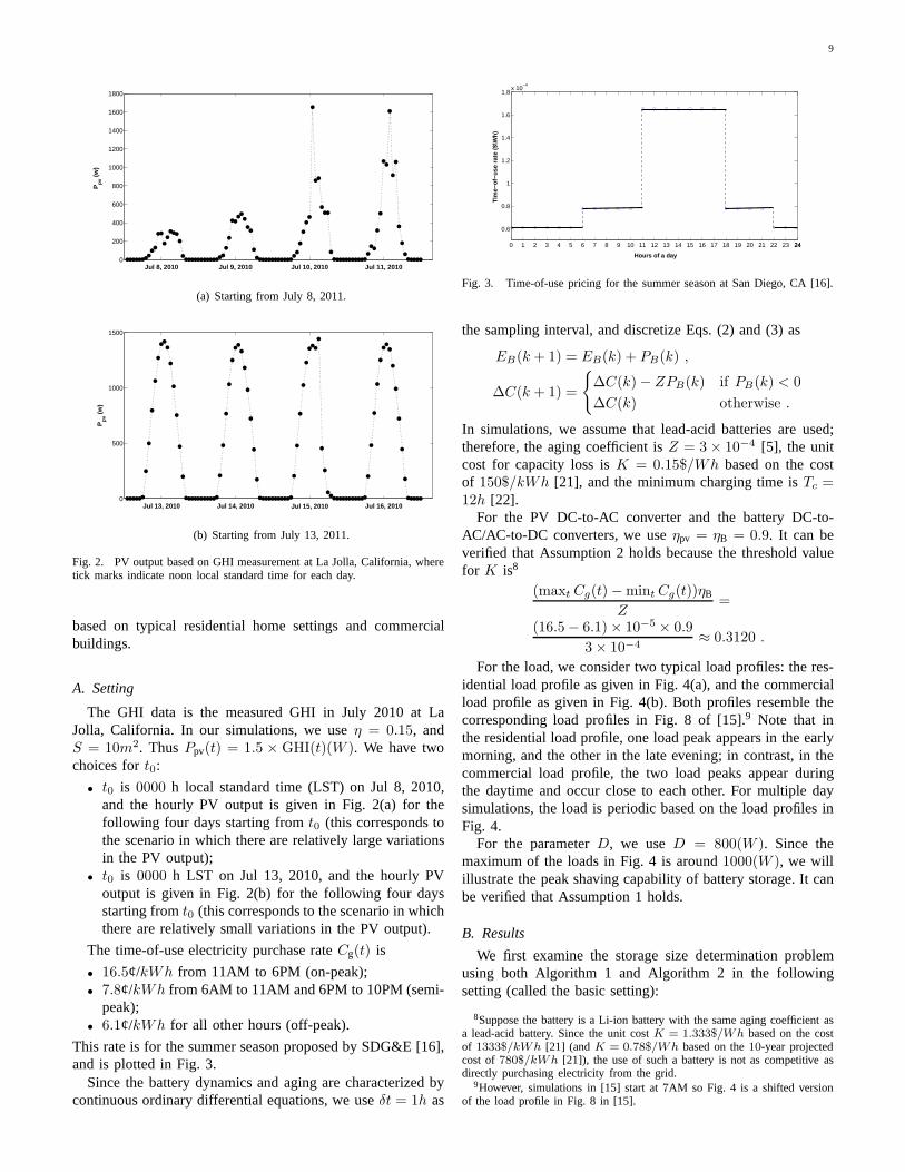
Fig. 2. PV output based on GHI measurement at La Jolla, California, wheretick marks indicate noon local standard time for each day.
based on typical residential home settings and commercialbuildings.
A. Setting
The GHI data is the measured GHI in July 2010 at LaJolla, California. In our simulations, we useη = 0.15, andS = 10m2. ThusPpv(t) = 1.5 × GHI(t)(W ). We have twochoices fort0:
• t0 is 0000 h local standard time (LST) on Jul 8, 2010,and the hourly PV output is given in Fig. 2(a) for thefollowing four days starting fromt0 (this corresponds tothe scenario in which there are relatively large variationsin the PV output);
• t0 is 0000 h LST on Jul 13, 2010, and the hourly PVoutput is given in Fig. 2(b) for the following four daysstarting fromt0 (this corresponds to the scenario in whichthere are relatively small variations in the PV output).
The time-of-use electricity purchase rateCg(t) is
• 16.5¢/kWh from 11AM to 6PM (on-peak);• 7.8¢/kWh from 6AM to 11AM and 6PM to 10PM (semi-
peak);• 6.1¢/kWh for all other hours (off-peak).
This rate is for the summer season proposed by SDG&E [16],and is plotted in Fig. 3.
Since the battery dynamics and aging are characterized bycontinuous ordinary differential equations, we useδt = 1h as
0 1 2 3 4 5 6 7 8 9 10 11 12 13 14 15 16 17 18 19 20 21 22 23 2424
0.6
0.8
1
1.2
1.4
1.6
1.8x 10
−4
Hours of a day
TIm
e−of
−use
rat
e ($
\Wh)
Fig. 3. Time-of-use pricing for the summer season at San Diego, CA [16].
the sampling interval, and discretize Eqs. (2) and (3) as
EB(k + 1) = EB(k) + PB(k) ,
∆C(k + 1) =
{
∆C(k)− ZPB(k) if PB(k) < 0
∆C(k) otherwise .
In simulations, we assume that lead-acid batteries are used;therefore, the aging coefficient isZ = 3 × 10⁻⁴ [5], the unitcost for capacity loss isK = 0.15$/Wh based on the costof 150$/kWh [21], and the minimum charging time isTc =12h [22].
For the PV DC-to-AC converter and the battery DC-to-AC/AC-to-DC converters, we useηpv = ηB = 0.9. It can beverified that Assumption 2 holds because the threshold valuefor K is8
(maxt Cg(t)−mint Cg(t))ηB
Z=
(16.5− 6.1)× 10−5 × 0.9
3× 10⁻⁴≈ 0.3120 .
For the load, we consider two typical load profiles: the res-idential load profile as given in Fig. 4(a), and the commercialload profile as given in Fig. 4(b). Both profiles resemble thecorresponding load profiles in Fig. 8 of [15].9 Note that inthe residential load profile, one load peak appears in the earlymorning, and the other in the late evening; in contrast, in thecommercial load profile, the two load peaks appear duringthe daytime and occur close to each other. For multiple daysimulations, the load is periodic based on the load profiles inFig. 4.
For the parameterD, we useD = 800(W ). Since themaximum of the loads in Fig. 4 is around1000(W ), we willillustrate the peak shaving capability of battery storage.It canbe verified that Assumption 1 holds.
B. Results
We first examine the storage size determination problemusing both Algorithm 1 and Algorithm 2 in the followingsetting (called the basic setting):
8Suppose the battery is a Li-ion battery with the same aging coefficient asa lead-acid battery. Since the unit costK = 1.333$/Wh based on the costof 1333$/kWh [21] (andK = 0.78$/Wh based on the10-year projectedcost of780$/kWh [21]), the use of such a battery is not as competitive asdirectly purchasing electricity from the grid.
9However, simulations in [15] start at7AM so Fig. 4 is a shifted versionof the load profile in Fig. 8 in [15].

10
0 1 2 3 4 5 6 7 8 9 10 11 12 13 14 15 16 17 18 19 20 21 22 23 24100
200
300
400
500
600
700
800
900
1000
Hours of a day
Load
(w
)
(a) Residential load averaged at536.8(W ).
0 1 2 3 4 5 6 7 8 9 10 11 12 13 14 15 16 17 18 19 20 21 22 23 24100
200
300
400
500
600
700
800
900
1000
1100
Hours of a day
Load
(w
)
(b) Commercial load averaged at485.6(W ).
Fig. 4. Typical residential and commercial load profiles.
• the cost minimization duration isT = 24(h),• t0 is 0000 h LST on Jul 13, 2010, and• the load is the residential load as shown in Fig. 4(a).
The lower and upper bounds in Proposition 5 are calculated as2667(Wh) and39269(Wh). When applying Algorithm 1, wechooseτcap= 10(Wh) andτcost= 10−4, and haveL = 3660.When running the algorithm,2327 optimization problems inEq. (8) have been solved. The maximum costJmax is −0.1921while the minimum cost is−0.3222, which is larger than thelower bound−2.5483 as calculated based on Proposition 4.The critical battery capacity is calculated to be16089(Wh).In contrast, only
⌈log2Cub
ref
τcap⌉+ 1 = 13
optimization problems in Eq. (8) are solved using Algorithm2while obtaining the same critical battery capacity.
Now we examine the solution to the optimization problemin Eq. (8) in the basic setting with the critical battery capacity16089(Wh). We solve the mixed integer programming prob-lem using the CPlex solver [20], and the objective function isJ(16089) = −0.3222. PB(t), EB(t) andC(t) are plotted inFig. 5(a). The plot ofC(t) is consistent with the fact that thereis capacity loss (i.e., the battery ages) only when the batteryis discharged. The capacity loss is around2.2(Wh), and
∆C(t0 + T )
Cref=
2.2
16089= 1.4× 10⁻⁴ ≈ 0 ,
which justifies the assumption we make when linearizing thenonlinear battery aging model in the Appendix. The dynamic
0 5 10 15 20−2000
0
2000
PB(W): Battery Charging/Discharging Profile
0 5 10 15 200
5000
10000
EB(Wh): Battery Charge Profile
0 5 10 15 201.6086
1.6087
1.6088
1.6089x 10
4 C(Wh): Capacity
(a)
0 5 10 15 200.5
1
1.5
2x 10
−4C
g($/Wh): Dynamic Pricing
0 5 10 15 20−2000
0
2000
PB(W): Battery Charging/Discharging Profile
0 5 10 15 20−4000
−2000
0
2000
Pload
(W): Load (solid red curve), and Pg(W): Net Power Purchase (dotted blue curve)
(b)
17 18 19 20 21 22 23−1000
−800
−600
−400
−200
0
200
400
600
800
1000P
load(W): Load (solid red curve), and P
g(W): Net Power Purchase (dotted blue curve)
(c)
Fig. 5. Solution to a typical setting in whicht0 is on Jul 13, 2010,T =24(h), the load is shown in Fig. 4(a), andCref = 16089(Wh).
pricing signalCg(t), PB(t), Pload(t) andPg(t) are plotted inFig. 5(b). From the second plot in Fig. 5(b), it can be observedthat the battery is charged when the time-of-use pricing is lowin the early morning, and is discharged when the time-of-usepricing is high. From the third plot in Fig. 5(b), it can beverified that, to minimize the cost, electricity is purchasedfrom the grid when the time-of-use pricing is low, and issold back to the grid when the time-of-use pricing is high;in addition, the peak demand in the late evening (that exceedsD = 800(W )) is shaved via battery discharging, as shown indetail in Fig. 5(c).
These observations also hold forT = 48(h). In this case, wechangeT to be48(h) in the basic setting, and solve the batterysizing problem. The critical battery capacity is calculated to beCc
ref = 16096(Wh). Now we examine the solution to the opti-

11
0 5 10 15 20 25 30 35 40 45−2000
0
2000
PB(W): Battery Charging/Discharging Profile
0 5 10 15 20 25 30 35 40 450
5000
10000
EB(W): Battery Charge Profile
0 5 10 15 20 25 30 35 40 451.609
1.6092
1.6094
1.6096x 10
4 C(Wh): Capacity
(a)
0 5 10 15 20 25 30 35 40 450.5
1
1.5
2x 10
−4C
g($/Wh): Dynamic Pricing
0 5 10 15 20 25 30 35 40 45−2000
0
2000
PB(W): Battery Charging/Discharging Profile
0 5 10 15 20 25 30 35 40 45−4000
−2000
0
2000
Pload
(W): Load (solid red curve), and Pg(W): Net Power Purchase (dotted blue curve)
(b)
Fig. 6. Solution to a typical setting in whicht0 is on Jul 13, 2010,T =48(h), the load is shown in Fig. 4(a), andCref = 16096(Wh).
mization problem in Eq. (8) with the critical battery capacity16096(Wh), and obtainJ(16096) = −0.6032. PB(t), EB(t),C(t) are plotted in Fig. 6(a), and the dynamic pricing signalCg(t), PB(t), Pload(t) andPg(t) are plotted in Fig. 6(b). Notethat the battery is gradually charged in the first half of eachday, and then gradually discharged in the second half to beempty at the end of each day, as shown in the second plot ofFig. 6(a).
To illustrate the peak shaving capability of the dynamicpricing signal as discussed in Remark 1, we change the loadto the commercial load as shown in Fig. 4(b) in the basicsetting, and solve the battery sizing problem. The criticalbattery capacity is calculated to beCc
ref = 13352(Wh), andJ(13352) = −0.1785. The dynamic pricing signalCg(t),PB(t), Pload(t) and Pg(t) are plotted in Fig. 7. For thecommercial load, the duration of the peak loads coincideswith that of the high price. To minimize the total cost, duringpeak times the battery is discharged, and the surplus electricityfrom PV after supplying the peak loads is sold back to thegrid resulting in a negative net power purchase from the grid,as shown in the third plot in Fig. 7. Therefore, unlike theresidential case, the high price indirectly forces the shaving ofthe peak loads.
Now we consider settings in which the load could be eitherresidential loads or commercial loads, the starting time couldbe on either Jul 8 or Jul 13, 2010, and the cost optimizationduration can be24(h), 48(h), 96(h). The results are shown inTables I and II. In Table I,t0 is on Jul 8, 2010, while in
0 5 10 15 200.5
1
1.5
2x 10
−4C
g($/Wh): Dynamic Pricing
0 5 10 15 20−4000
−2000
0
2000
PB(W): Battery Charging/Discharging Profile
0 5 10 15 20−4000
−2000
0
2000
Pload
(W): Load (solid red curve), and Pg(W): Net Power Purchase (dotted blue curve)
Fig. 7. Solution to a typical setting in whicht0 is on Jul 13, 2010,T =24(h), the load is shown in Fig. 4(b), andCref = 13352(Wh).
Table II, t0 is on Jul 13, 2010. In the pair(24, R), 24 refersto the cost optimization duration, andR stands for residentialloads; in the pair(24, C), C stands for commercial loads.
We first focus on the effects of load types. From Tables Iand II, the commercial load tends to result in a higher cost(even though the average cost of the commercial load issmaller than that of the residential load) because the peaksofthe commercial load coincide with the high price. When thereis a relatively large variation of PV generation, commercialloads tend to result in larger optimum battery capacityCc
ref asshown in Table I, presumably because the peak load occursduring the peak pricing period and reductions in PV productionhave to be balanced by additional battery capacity; when thereis a relatively small variation of PV generation, residentialloads tend to result in larger optimum battery capacityCc
ref asshown in Table II. Ift0 is on Jul 8, 2010, the PV generationis relatively lower than the scenario in whicht0 is on Jul 13,2010, and as a result, the battery capacity is smaller and thecost is higher. This is because it is more profitable to storePV generated electricity than grid purchased electricity.FromTables I and II, it can be observed that the cost optimizationduration has relatively larger impact on the battery capacityfor residential loads, and relatively less impact for commercialloads.
In Tables I and II, the rowJmax corresponds to the cost inthe scenario without batteries, the rowJ(Cc
ref) corresponds tothe cost in the scenario with batteries of capacityCc
ref, and therow Savings10 corresponds toJmax− J(Cc
ref). For Table I, wecan also calculate the relative percentage of savings usingtheformula Jmax−J(Cc
ref)Jmax
, and get the rowPercentage. One obser-vation is that the relative savings by using batteries increase asthe cost optimization duration increases. For example, whenT = 96(h) and the load type is residential,16.10% cost can besaved when a battery of capacity18320(Wh) is used; whenT = 96(h) and the load type is commercial,25.79% costcan be saved when a battery of capacity15747(Wh) is used.This clearly shows the benefits of utilizing batteries in grid-connected PV systems. In Table II, only the absolute savingsare shown since negative costs are involved.
10Note that in Table II, part of the costs are negative. Therefore, the word“Earnings” might be more appropriate than “Savings”.

12
TABLE ISIMULATION RESULTS FORt0 ON JUL 8, 2011
(24, R) (48, R) (96, R) (24, C) (48, C) (96, C)Cc
ref 6891 7854 18320 8747 13089 15747J(Cc
ref) 0.8390 1.5287 1.9016 0.9802 1.7572 2.3060Jmax 0.9212 1.7027 2.2666 1.1314 2.1232 3.1076
Savings 0.0822 0.1740 0.3650 0.1512 0.3660 0.8016Percentage 8.92% 10.22% 16.10% 13.36% 17.24% 25.79%
TABLE IISIMULATION RESULTS FORt0 ON JUL 13, 2011
(24, R) (48, R) (96, R) (24, C) (48, C) (96, C)Cc
ref 16089 16096 70209 13352 17363 32910J(Cc
ref) -0.3222 -0.6032 -0.9930 -0.1785 -0.3721 -0.5866Jmax -0.1921 -0.3395 -0.4649 0.0181 0.0810 0.3761
Savings 0.1301 0.2637 0.5281 0.1966 0.4531 0.9627
VI. CONCLUSIONS
In this paper, we studied the problem of determining thesize of battery storage for grid-connected PV systems. Weproposed lower and upper bounds on the storage size, andintroduced an efficient algorithm for calculating the storagesize. In our analysis, the conversion efficiency of the PVDC-to-AC converter and the battery DC-to-AC and AC-to-DC converters is assumed to be a constant. We acknowledgethat this is not the case in the current practice, in whichthe efficiency of converters depends on the input power ina nonlinear fashion [5]. This will be part of our future work.In addition, we would like to extend the results to distributedrenewable energy storage systems, and generalize our settingby taking into account stochastic PV generation.
APPENDIX
Derivation of the Simplified Battery Aging ModelEqs. (11) and (12) in [5] are used to model the battery
capacity loss, and are combined and rewritten below using thenotation in this work:
C(t+δt)−C(t) = −Cref×Z×(EB(t)
C(t)−EB(t+ δt)
C(t+ δt)) . (15)
If δt is very small, thenC(t+δt) ≈ C(t). Therefore,EB(t)C(t) −
EB(t+δt)C(t+δt) ≈ −PB(t)δt
C(t) . If we plug in the approximation, divideδt on both sides of Eq. (15), and letδt goes to0, then wehave
dC(t)
dt= Cref × Z ×
PB(t)
C(t). (16)
This holds only ifPB(t) < 0 as in [5], i.e., there could becapacity loss only when discharging the battery.
Since Eq. (16) is a nonlinear equation, it is difficult to solve.Let ∆C(t) = Cref − C(t), then Eq. (16) can be rewritten as
d∆C(t)
dt= −Z ×
PB(t)
1− ∆C(t)Cref
. (17)
If t is much shorter than the life time of the battery, then thepercentage of the battery capacity loss∆C(t)
Crefis very close to
0. Therefore, Eq. (17) can be simplified to the following linearODE
d∆C(t)
dt= −Z × PB(t) ,
whenPB(t) < 0. If PB(t) ≥ 0, there is no capacity loss, i.e.,
dC(t)
dt= 0 .
REFERENCES
[1] H. Kanchev, D. Lu, F. COLAS, V. Lazarov, and B. Francois, “Energymanagement and operational planning of a microgrid with a PV-basedactive generator for smart grid applications,”IEEE Transactions onIndustrial Electronics, 2011.
[2] S. Teleke, M. E. Baran, S. Bhattacharya, and A. Q. Huang, “Rule-basedcontrol of battery energy storage for dispatching intermittent renewablesources,”IEEE Transactions on Sustainable Energy, vol. 1, pp. 117–124,2010.
[3] M. Lafoz, L. Garcia-Tabares, and M. Blanco, “Energy managementin solar photovoltaic plants based on ESS,” inPower Electronics andMotion Control Conference, Sep. 2008, pp. 2481–2486.
[4] W. A. Omran, M. Kazerani, and M. M. A. Salama, “Investigationof methods for reduction of power fluctuations generated from largegrid-connected photovoltaic systems,”IEEE Transactions on EnergyConversion, vol. 26, pp. 318–327, Mar. 2011.
[5] Y. Riffonneau, S. Bacha, F. Barruel, and S. Ploix, “Optimal powerflow management for grid connected PV systems with batteries,” IEEETransactions on Sustainable Energy, 2011.
[6] IEEE Recommended Practice for Sizing Lead-Acid Batteries for Stand-Alone Photovoltaic (PV) Systems, IEEE Std 1013-2007, IEEE, 2007.
[7] G. Shrestha and L. Goel, “A study on optimal sizing of stand-alone pho-tovoltaic stations,”IEEE Transactions on Energy Conversion, vol. 13,pp. 373–378, Dec. 1998.
[8] M. Akatsuka, R. Hara, H. Kita, T. Ito, Y. Ueda, and Y. Saito, “Esti-mation of battery capacity for suppression of a PV power plant outputfluctuation,” in IEEE Photovoltaic Specialists Conference (PVSC), Jun.2010, pp. 540–543.
[9] X. Wang, D. M. Vilathgamuwa, and S. Choi, “Determinationof batterystorage capacity in energy buffer for wind farm,”IEEE Transactions onEnergy Conversion, vol. 23, pp. 868–878, Sep. 2008.
[10] T. Brekken, A. Yokochi, A. von Jouanne, Z. Yen, H. Hapke,andD. Halamay, “Optimal energy storage sizing and control for wind powerapplications,”IEEE Transactions on Sustainable Energy, vol. 2, pp. 69–77, Jan. 2011.
[11] Q. Li, S. S. Choi, Y. Yuan, and D. L. Yao, “On the determination ofbattery energy storage capacity and short-term power dispatch of a windfarm,” IEEE Transactions on Sustainable Energy, vol. 2, pp. 148–158,Apr. 2011.
[12] B. Borowy and Z. Salameh, “Methodology for optimally sizing thecombination of a battery bank and pv array in a wind/PV hybridsystem,”IEEE Transactions on Energy Conversion, vol. 11, pp. 367–375, Jun.1996.

13
[13] R. Chedid and S. Rahman, “Unit sizing and control of hybrid wind-solarpower systems,”IEEE Transactions on Energy Conversion, vol. 12, pp.79–85, Mar. 1997.
[14] E. I. Vrettos and S. A. Papathanassiou, “Operating policy and optimalsizing of a high penetration res-bess system for small isolated grids,”IEEE Transactions on Energy Conversion, 2011.
[15] M. H. Rahman and S. Yamashiro, “Novel distributed powergeneratingsystem of PV-ECaSS using solar energy estimation,”IEEE Transactionson Energy Conversion, vol. 22, pp. 358–367, Jun. 2007.
[16] SDG&E proposal to charge electric rates for different timesof the day: The devil lurks in the details. [Online]. Available:http://www.ucan.org/energy/electricity/sdgeproposalchargeelectric rates different times day devil lurks details
[17] M. Ceraolo, “New dynamical models of lead-acid batteries,” IeeeTransactions On Power Systems, vol. 15, pp. 1184–1190, 2000.
[18] S. Barsali and M. Ceraolo, “Dynamical models of lead-acid batteries:Implementation issues,”IEEE Transactions On Energy Conversion,vol. 17, pp. 16–23, Mar. 2002.
[19] A. E. Bryson and Y.-C. Ho,Applied Optimal Control: Optimization,Estimation and Control. New York, USA: Taylor & Francis, 1975.
[20] IBM ILOG CPLEX Optimizer. [Online]. Available:http://www-01.ibm.com/software/integration/optimization/cplex-optimizer
[21] D. Ton, G. H. Peek, C. Hanley, and J. Boyes, “Solar energygridintegration systems — energy storage,” Sandia National Lab, Tech. Rep.,2008.
[22] Charging information for lead acid batteries. [Online]. Available:http://batteryuniversity.com/learn/article/chargingthe lead acid battery