Revista Facultad de Ingeniería, Universidad de Antioquia, No.99, pp. 32-43, Apr-Jun 2021

Determination of photovoltaic power bymodeling solar radiation with Gammadistribution in the CEDER microgridDeterminación de potencia fotovoltaica por modelación de radiación solar con distribuciónGamma en microred CEDERRaúl Alberto López-Meraz 1, Luis Hernández-Callejo 2*, Luis Omar Jamed-Boza 1, VictorAlonso-Gómez3

1Unidad de Ingenierías y Ciencias Químicas, Universidad Veracruzana. Circuito Universitario Gonzalo Aguirre Beltrán s/n.C. P. 9100. Xalapa, México.2Departamento Ingeniería Agrícola y Forestal, Universidad de Valladolid. Campus Universitario Duques de Soria. C. P.42004. Soria, Spain.3Departamento de Física Aplicada, Universidad de Valladolid. Campus Universitario Duques de Soria. C. P. 42004. Soria,Spain.

CITE THIS ARTICLE AS:R. A. López, L. Hernández, L.O. Jamed and V. A. Gómez.”Determinación de potenciafotovoltaica por modelación deradiación solar condistribución Gamma enmicrored CEDER”, RevistaFacultad de IngenieríaUniversidad de Antioquia, no.99, pp. 32-43, Apr-Jun 2021.[Online]. Available: https://www.doi.org/10.17533/udea.redin.20200579

ARTICLE INFO:Received: November 18, 2019Accepted: May 19, 2020Available online: May 19, 2020

KEYWORDS:Gamma distribution;microgrid; solar radiation;simulated power

Distribución gamma;microrred; radiación solar;potencia simulada

ABSTRACT: The article proposes a methodology applicable to any photovoltaic (PV) plantto obtain an approximation of the monthly production of solar array power. The analysiswas carried out in seven systems, of different technologies and capacities, connectedto the microgrid of the Center for the Development of Renewable Energies (CEDER)belonging to the Center for Energy, Environmental and Technological Research (CIEMAT)in Soria, Spain. The proposal simulates radiation by combining and crossing two Gammaprobability distributions, representing the days with the best and worst solar resources,respectively. As a result, a matrix was created with 12 variables that define the monthlybehavior of the radiation. On the other hand, the granularity of the PV generationwas homogenized to know it at any moment through polynomial functions. Once bothcharacterizations were known, it was possible to predict the monthly power of each PVarray. The methodology has been validated with the measurement approximation index,developed in the text, and with specialized software. The results presented will help inthe dimensioning of a backup model and will collaborate in the adequate managementof energy.

RESUMEN: El artículo propone una metodología aplicable a cualquier planta fotovoltaica(FV) para obtener un acercamiento de la producción mensual de potencia de arreglossolares. El análisis se llevó a cabo en siete sistemas, de tecnologías y capacidadesdiferentes, conectados a la microred del Centro de Desarrollo de Energías Renovables(CEDER) perteneciente al Centro de Investigaciones Energéticas, Medioambientales yTecnológicas (CIEMAT) en Soria, España. La propuesta simula la radiación mediantela combinación y cruce de dos distribuciones de probabilidad Gamma, representandolos días de mejor y peor recurso solar, respectivamente. Como resultado, se creó unamatriz con 12 variables que definen el comportamientomensual de la radiación. Por otrolado, se homogenizó la granularidad de la generación FV para conocerla en cualquierinstante a través de funciones polinomiales. Conocidas ambas caracterizaciones selogró predecir la potencia mensual de cada conjunto FV. Lametodología ha sido validadacon el índice de acercamiento a las mediciones, desarrollado en el texto, y con softwareespecializado. Los resultados presentados ayudarán en el dimensionamiento de unmodelo de respaldo y colaborarán en la gestión adecuada de la energía.

1. Introduction

In recent years, humanity demands a large amount ofelectricity; Latin America, for example, has a growth rateof 5% [1, 2]. The use of raw materials, the cornerstone oftechnical progress in the middle of the twentieth century,

32

* Corresponding author: Luis Hernández Callejo

E-mail: luis.hernandez.callejo.uva.es

ISSN 0120-6230

e-ISSN 2422-2844

DOI: 10.17533/udea.redin.2020057932

R. A. López-Meraz et al., Revista Facultad de Ingeniería, Universidad de Antioquia, No. 99, pp. 32-43, 2021

to satisfy consumption contributes to the erosion of natureand to promote anthropogenic climate change. In thisscenario, renewable energies are incorporated as a newactor trying to cover what society requests in a lesspolluting way.

There are essentially two schemes where renewableproduction is present. The first, distributed energyresources (DER), includes different aspects such asgeneration, storage, and demand response; an interestingcase study of the latter aspect is discussed in [3]. Onthe other hand, the new paradigms and the latestdevelopments in the electricity sector are based on theintroduction of distributed generation (DG), which is aphilosophy where energy is not produced exclusively inlarge centralized plants, if not also in smaller locationstaking advantage of local conditions in order to minimizetransmission/distribution losses, as well as optimizingproduction and consumption. This represents anopportunity for renewable energies, where elementssuch as photovoltaic panels and wind turbines, scatteredthroughout the network, supply installations on-site orsell energy depending on their generation/consumptionconditions [4]. Consequently, according to data from theEuropean Commission, DG penetration into the Europeannetwork is estimated to be around 20-25% of the totalgeneration by 2020, and by 2030 this figure will be set at30-35%.

However, electricity generation based on renewableresources, mainly wind and solar, has highlightedadditional challenges in the management of the electricitysystem, primarily due to the dispersion of this typeof generators, the energy of changing output, and theinefficient coordination of the conditions of the electricalgrid. These complications have created technicalobstacles such as energy management, architecturedesign of electrical systems, voltage, and frequencysupport, means of protection and low voltage aspects [5].They also increase the computation difficulty due to themore complex and asymmetrical probability distributionsassociated with the intermittent plant [6]. In addition, giventhe considerable number of plants, there is the challengeof obtaining energy production data in real-time [7]. Otherrelevant issues are the difference, in statistical terms,between the availability of intermittent source resourcesand conventional generation, as well as the contributionthat oscillating production can make to satisfy the peakdemand of the system while maintaining its reliability [8].

Complications caused by photovoltaic generation aredependent on solar radiation, promoting the interest ofdifferent studies to find a probability model that bestfits the measurements. Thus, [9] performs a radiationanalysis in Taiwan with Weibull distributions, logistics,

Normal, and logNormal without detecting bimodalbehavior. Additionally, in [10], they claim that the variationin radiation does not follow bimodal behavior. In addition,the study of the behavior of global radiation in the M’Silaregion (Algeria) is developed in [11], using six individualfrequency distributions finding that theWeibull distributionbest matches the measured data for all months, that is,they did not find a bimodal fit either. On the other hand,[12, 13] argue bimodal performance in the distribution ofradiation observations, [14] they analyze solar radiationrecords and similarly detect bimodal behavior in thedistribution of data for intervals less than 60 minutes.

Given the importance of photovoltaic generation, thiswork attempts to approximate the quantification of thereal power supplied from photovoltaic arrays (PVA) tothe microgrid of the Center for the Development ofRenewable Energies (CEDER) belonging to the Centerfor Environmental and Technological Energy Research(CIEMAT) located in Soria, Spain. The analysis focuseson modeling, on a monthly basis, the radiation withthe Gamma probability distribution and, at the sametime, finding relationships between it and the individualproduction in days with the best solar resource finding theprofile of each PVA.

The text is made up of four sections. It begins withthe description of the components of the case study andthe elements for measuring the information. Sectionthree shows the methodology for modeling radiationand determining the association functions between thesolar resource and the PV power. Point four exposes theresults of the characterization of the monthly radiationand the representative functions of the behavior of the PVAvalidated by the JMP version 8.0.2 software as well as bythe measurement approach index (Ipm), in addition, thesimulation of the monthly power of the PVAs is presentedwith the help of Matlab R2015a, it is important to notethat some of the results presented in this article arepublished in [15]. Finally, the most relevant conclusionsare presented.

2. Case study

Of all the manageable components of CEDER’s microgrid,this work focuses on a photovoltaic generation whose totalpeak power is of 78 kW. As shown in Figure 1, the PVAsare assembled into five generation groups [16], three ofthem are on roofs and the rest are at floor level.

The five solar sets are briefly described.

1. Turbine zone: the installation consists of 16 kWdistributed in 64 panels of monocrystalline siliconof 250 W each, housed in two structures, forming

33

R. A. López-Meraz et al., Revista Facultad de Ingeniería, Universidad de Antioquia, No. 99, pp. 32-43, 2021

Figure 1 Distribution of RES in CEDER microgrid

four series (two series per structure) of 16 panelseach. The output is connected to a 15 kW inverter andconnected to the three-phase network

2. Roof photovoltaic building E01 Arfrisol: this generatorof 12 kW is made up of 80 monocrystalline siliconpanels of 150 W, distributed in five series of 16modules each. They arrive at a three-phase inverterof 10 kW.

3. Building roof E03: the arrangement has a power of12.5 kW in 54 panels of monocrystalline silicon of twodifferent brands. Some give 230 W and the other 240W,with very similar characteristics, there are 36 of thefirst type and 18 of the second. They are connected toa 10 kW three-phase inverter.

4. Building roof E09: plant divided into two groups, oneof 84 and the other of 154 modules, arranged in 17series of 14 panels each, with a peak capacity of 23.5kW. The 238 panels are thin film (CdTe) with a powerof 97 W and discharge to a three-phase inverter of 20kW.

5. PEPA III: consists of three facilities called park 1,park 2, and park 3. They deliver their generation tosingle-phase inverters of 5 kW, connecting each parkto a phase. Structures 2 and 3 are the same. Park1: consists of 24 modules of polycrystalline silicondistributed in four series of 6 panels, its peak poweris 5 kW. Parks 2 and 3: generators of 32 modulesof monocrystalline silicon of 140 W, grouped in fourseries of 8 panels, providing a maximum power of 4.5kW.

Due to the need for higher resolution data, themeasurement of the solar resource in situ was performedwith a station belonging to the Response SurfaceRadiation Network (BSRN) whose purpose is to detect

relevant changes of this variable on Earth that are relatedto climatic changes [17]. The equipment is located inbuilding E01 and measures various parameters such asUVA, UVB, infrared, etc.; however, only global radiation isof interest for this work. The information was acquiredevery five minutes in the period from November 1st,2010 to May 15th, 2015, with a total of 442,905 records.The monitoring of the power injection produced by thephotovoltaic plants to the CEDER network was donethrough intelligent meters; their acquisition is exportedto a database formed at different granularity, 5 minutes,and hourly, respectively. The correspondence between themeasuring equipment and its respective PVA is presentedin Table 1.

Table 1 Smart Meters with your generation plant

Smart meter PV generatorAE1037 (5) Park 1AE1038 (5) Park 2AE1044 (5) Park 3AE2000 (2) E01 ArfrisolAE2005 (3) E03AE2010 (1) Turbine zoneAE4360 (4) E09

3. Materials and methods

Before visualizing the developed methodology, Figure 2,as an example, presents the evolution, without processing,of the radiation in January. As can be seen, the completehistory of the measurement records was not available. Inaddition, it is easy to observe the oscillation in the valuesof the solar resource for different days of the month.

In order to facilitate the understanding of the methodology

34

R. A. López-Meraz et al., Revista Facultad de Ingeniería, Universidad de Antioquia, No. 99, pp. 32-43, 2021

Figure 2 Behavior of radiation data for the month of January

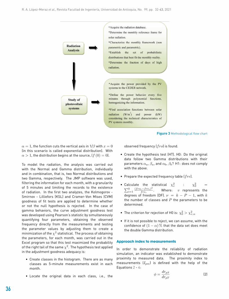
developed and the variables involved in it, Figure 3 showsthe corresponding flow chart. Lines below deepen thesesections.

3.1 Radiation modeling

Gamma distribution

Since the behavior of a random variable is described byits probability distribution, the closest to the measuredmonthly radiation was sought. Among the most useful forrepresenting atmospheric parameters is Gamma, whichis suitable for modeling when bias, positive asymmetry,and time is involved. Such environmental measuresinclude precipitation, wind speed, and relative humidity, allrestricted by a physical limit.

In short, the Gamma distribution is the one where therandom variable occurs α times until there is a certainevent [18]. Its density function is given by Equation 1:

f(x) =

{1

βαΓ(α)xα−1e

−xβ , for x > 0;α, β > 0

0(1)

Where α is the shape parameter and β the scaleparameter. When large values of α occur, distributionsresult in less bias and a shift in the probability of densityto the right. For very large values of α (50 < α < 100)the distribution approximates, in its form, the normal.The parameter β “extends” or “squeezes” the function tothe right or to the left, when is large, the curve is moreelongated [19]. The main cases of this distribution are asfollows: with α < 1, it is strongly skewed to the right. For

35

R. A. López-Meraz et al., Revista Facultad de Ingeniería, Universidad de Antioquia, No. 99, pp. 32-43, 2021

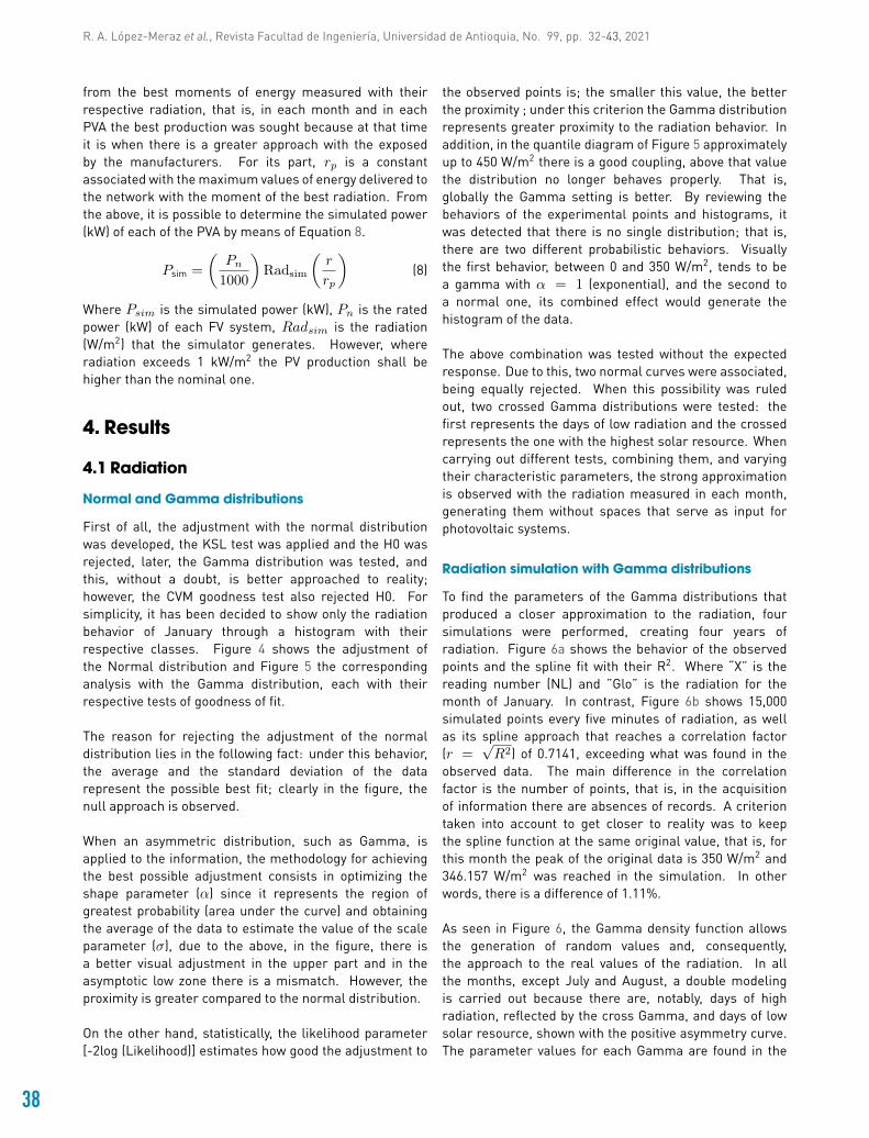
Figure 3 Methodological flow chart

α = 1, the function cuts the vertical axis in 1/β with x = 0(in this scenario is called exponential distribution). Withα > 1, the distribution begins at the source, (f (0) = 0).

To model the radiation, the analysis was carried outwith the Normal and Gamma distribution, individuallyand in combination, that is, two Normal distributions andtwo Gamma, respectively. The JMP software was used,filtering the information for each month, with a granularityof 5 minutes and limiting the records to the existenceof radiation. In the first two analyzes, the Kolmogorov -Smirnov - Lilliefors (KSL) and Cramer-Von Mises (CVM)goodness of fit tests are applied to determine whetheror not the null hypothesis is rejected. In the case ofgamma behaviors, the curve adjustment goodness testwas developed using Pearson’s statistic by simultaneouslyquantifying four parameters, obtaining the observedfrequency directly from the measurements and testingthe parameter values by adjusting them to create aminimization of the χ2 statistical. The process of obtainingthe parameters, for each month, was carried out in theExcel program so that this test maximized the probabilityof the right tail of the same χ2. The hypothesis test appliedin the adjustment goodness adequacy is:

• Create classes in the histogram. There are as manyclasses as 5-minute measurements exist in eachmonth.

• Locate the original data in each class, i.e., the

observed frequency (fro) is found.

• Create the hypothesis test (HT). H0: Do the originaldata follow two Gamma distributions with theirparameters αa, βa, and αb, βb? H1: does not complywith the above.

• Prepare the expected frequency table (fre).

• Calculate the statistical χ2v : χ2

0 =∑ki=1

(froi−frei)2

frei. Where: v represents the

degrees of freedom (DF). ν = k − P − 1, with kthe number of classes and P the parameters to bedetermined.

• The criterion for rejection of H0 is: χ20 > χ2

v,α

• If it is not possible to reject, we can assume, with theconfidence of (1− α)% that the data set does meetthe double Gamma distribution.

Approach index to measurements

In order to demonstrate the reliability of radiationsimulation, an indicator was established to demonstrateproximity to measured data. The proximity index tomeasurements (Ipm) is defined with the help of theEquations 2 - 4:

ϕ =drpSdrpT

(2)

36

R. A. López-Meraz et al., Revista Facultad de Ingeniería, Universidad de Antioquia, No. 99, pp. 32-43, 2021

fdif = (ϕ− 1)

[fdaTfdaS

](f) (3)

Ipm = (1− fdif ) (100) (4)

Where ϕ is the ratio of the simulated reference splines(drpS ) and the theoretical one obtained with theinformation (drpT ) [20], fdif is the fraction of differenceand is a function of the fractions of days of good theoreticalradiation (fdaT ), of that provided by the simulation (fdaS )and of the random factor f = 1

σ2 where σ2 is the varianceof the combined simulation of the crossed gamma adjustedto the nearest integer.

A fraction of high radiation days

To determine the percentage of days with better radiationwere found two monthly values, these are: referencedistance (rd) represented by the radiation peak measuredfrom the spline reference frame and high distance (hd)estimated from the points observed with the highestmagnitude. In this way, the fraction of high radiation dayswas found: Fhr = rd

hd . When there are days of higherradiation, the spline ”rises”, thus both distances are close,indicating the presence of a greater number of days wherethe radiation is considered high.

Radiation conformation

The structure of the monthly radiation matrix (Rad), whichrepresents the 12 months of the year, consists of 192elements consisting of 12 rows and 16 columns. Itsconfiguration is as follows: the elements located in thefirst six positions correspond to the β’s of the polynomialsof each month, obtained from the characterization ofradiation [20]; the number of days (nd) is found in columnseven, the following three parameters are the maximumreached value, that is, the peak radiation (pr), themagnitude of the reference spline (rd) and the minimumvalue (mv). The start (sr) and end (er) readings of theradiation measurement form columns eleven and twelveand the last four are the coefficients of α and β of thetwo Gammas distributions; in this way, αa and βa equalthe simulation on sunny days and αb and βb represent thecloudy days.

3.2 Photovoltaic systems

Standardization of PV power

The analysis of the solar systems was carried out intwo parts, the first, directly relating the radiation, onthe days with the best resource (the PV systems in theirdesign are independent of environmental variations in theiroperation), and the production of themeasured AFVs by thefollowing equipment: AE1037, AE1038, AE1044, AE2000,

and AE2005. It is important to remember that the systemsmeasured by AE1038 and AE1044 correspond to exactly thesame facilities in their architecture and type of technology.However, energy variations were found in four months, andconsequently, the analysis of the park two only covers themonths of July, August, September, and October. Thesecond section corresponded to the characterization ofthe power obtained by the meters AE2010 and AE4360;different polynomial adjustments without transformationwere tested finding few correlations, so it was decidedto analyze the transformation with logarithm base 2 inthe response (power) to improve the experimental spaceof measurements to represent its behavior clearly. Thereason for using transformation with base logarithm 2instead of the traditional natural logarithm was to observeimprovement in correlation by reducing the base exponente to 2, better adjusting both curves to the “m” typecharacteristic. The statistical criterion of choosing base 2is supported on the Box-Cox Y Transformation techniquethat minimizes the sum of squares of the error in theresponse [21]. Equation 5 shows the arrangement of Boxand Cox.

YT =yλ − 1

λyλ−1(5)

Where y is the geometric mean and λ is an exponent thatvaries between -2 to 2.

In this way it is possible to determine the behaviorbetween the generated energy and the measuredradiation, homogenizing the information every fiveminutes.

Association Functions (r’s)

The monthly relationship between the measurements ofenergy produced and radiation received is found withpolynomial functions in the form of reasons that allow itto be segmented to any granularity. Since each PV systemhas its nominal power referenced at 1,000 W/m2, the peakfunctions (rp) are obtained. Thus, we have Equations 6 and7:

r =E

R(6)

rp =Ep

Rp(7)

Where r and rp are the associations between the energyproduced and the radiation at a certain instant and in peakconditions,E is the energy measured by the smart metersin Table 1,R represents themeasured radiation,Ep andRp

describe the energy and radiation in maximum conditions.It is worthmentioning that in the PVAs of higher production,the functions r and rp were converted again with the helpof the following property of the logarithms: loga N = lnN

lna.

Where a is the basis of logarithm and N is the numberto be transformed. Of this mode r is a function obtained

37

R. A. López-Meraz et al., Revista Facultad de Ingeniería, Universidad de Antioquia, No. 99, pp. 32-43, 2021

from the best moments of energy measured with theirrespective radiation, that is, in each month and in eachPVA the best production was sought because at that timeit is when there is a greater approach with the exposedby the manufacturers. For its part, rp is a constantassociated with themaximum values of energy delivered tothe network with the moment of the best radiation. Fromthe above, it is possible to determine the simulated power(kW) of each of the PVA by means of Equation 8.

Psim =

(Pn

1000

)Radsim

(r

rp

)(8)

Where Psim is the simulated power (kW), Pn is the ratedpower (kW) of each FV system, Radsim is the radiation(W/m2) that the simulator generates. However, whereradiation exceeds 1 kW/m2 the PV production shall behigher than the nominal one.

4. Results

4.1 Radiation

Normal and Gamma distributions

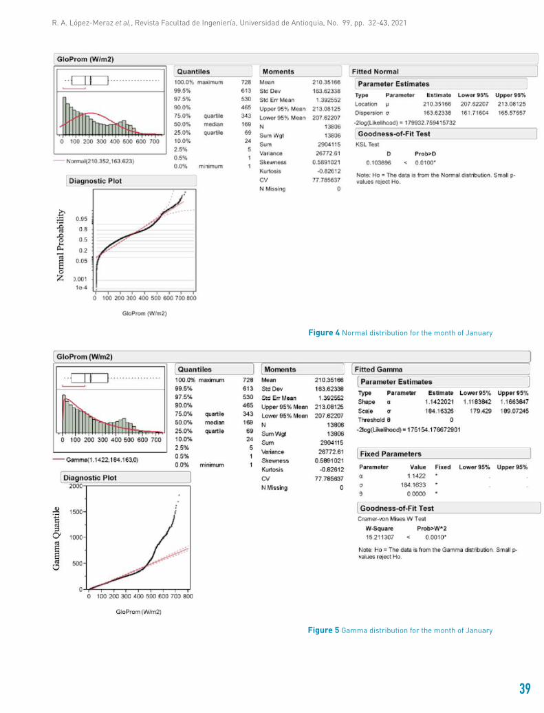
First of all, the adjustment with the normal distributionwas developed, the KSL test was applied and the H0 wasrejected, later, the Gamma distribution was tested, andthis, without a doubt, is better approached to reality;however, the CVM goodness test also rejected H0. Forsimplicity, it has been decided to show only the radiationbehavior of January through a histogram with theirrespective classes. Figure 4 shows the adjustment ofthe Normal distribution and Figure 5 the correspondinganalysis with the Gamma distribution, each with theirrespective tests of goodness of fit.

The reason for rejecting the adjustment of the normaldistribution lies in the following fact: under this behavior,the average and the standard deviation of the datarepresent the possible best fit; clearly in the figure, thenull approach is observed.

When an asymmetric distribution, such as Gamma, isapplied to the information, the methodology for achievingthe best possible adjustment consists in optimizing theshape parameter (α) since it represents the region ofgreatest probability (area under the curve) and obtainingthe average of the data to estimate the value of the scaleparameter (σ), due to the above, in the figure, there isa better visual adjustment in the upper part and in theasymptotic low zone there is a mismatch. However, theproximity is greater compared to the normal distribution.

On the other hand, statistically, the likelihood parameter[-2log (Likelihood)] estimates how good the adjustment to

the observed points is; the smaller this value, the betterthe proximity ; under this criterion the Gamma distributionrepresents greater proximity to the radiation behavior. Inaddition, in the quantile diagram of Figure 5 approximatelyup to 450 W/m2 there is a good coupling, above that valuethe distribution no longer behaves properly. That is,globally the Gamma setting is better. By reviewing thebehaviors of the experimental points and histograms, itwas detected that there is no single distribution; that is,there are two different probabilistic behaviors. Visuallythe first behavior, between 0 and 350 W/m2, tends to bea gamma with α = 1 (exponential), and the second toa normal one, its combined effect would generate thehistogram of the data.

The above combination was tested without the expectedresponse. Due to this, two normal curves were associated,being equally rejected. When this possibility was ruledout, two crossed Gamma distributions were tested: thefirst represents the days of low radiation and the crossedrepresents the one with the highest solar resource. Whencarrying out different tests, combining them, and varyingtheir characteristic parameters, the strong approximationis observed with the radiation measured in each month,generating them without spaces that serve as input forphotovoltaic systems.

Radiation simulation with Gamma distributions

To find the parameters of the Gamma distributions thatproduced a closer approximation to the radiation, foursimulations were performed, creating four years ofradiation. Figure 6a shows the behavior of the observedpoints and the spline fit with their R2. Where “X” is thereading number (NL) and ”Glo” is the radiation for themonth of January. In contrast, Figure 6b shows 15,000simulated points every five minutes of radiation, as wellas its spline approach that reaches a correlation factor(r =

√R2) of 0.7141, exceeding what was found in the

observed data. The main difference in the correlationfactor is the number of points, that is, in the acquisitionof information there are absences of records. A criteriontaken into account to get closer to reality was to keepthe spline function at the same original value, that is, forthis month the peak of the original data is 350 W/m2 and346.157 W/m2 was reached in the simulation. In otherwords, there is a difference of 1.11%.

As seen in Figure 6, the Gamma density function allowsthe generation of random values and, consequently,the approach to the real values of the radiation. In allthe months, except July and August, a double modelingis carried out because there are, notably, days of highradiation, reflected by the cross Gamma, and days of lowsolar resource, shown with the positive asymmetry curve.The parameter values for each Gamma are found in the

38

R. A. López-Meraz et al., Revista Facultad de Ingeniería, Universidad de Antioquia, No. 99, pp. 32-43, 2021

Figure 4 Normal distribution for the month of January

Figure 5 Gamma distribution for the month of January

39

R. A. López-Meraz et al., Revista Facultad de Ingeniería, Universidad de Antioquia, No. 99, pp. 32-43, 2021

(a)

(b)

Figure 6 (a) Radiation measured in the month of January. (b)Radiation simulation with two Gamma distributions with their

corresponding spline fit for the month of January

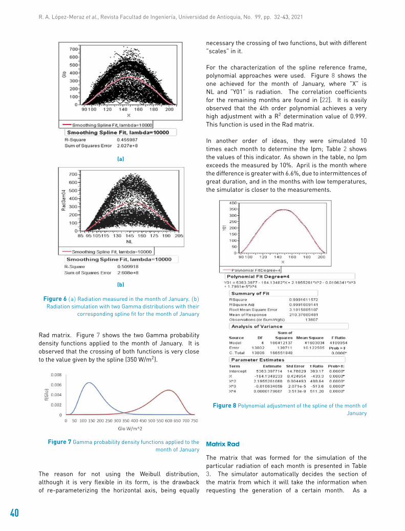
Rad matrix. Figure 7 shows the two Gamma probabilitydensity functions applied to the month of January. It isobserved that the crossing of both functions is very closeto the value given by the spline (350 W/m2).

Figure 7 Gamma probability density functions applied to themonth of January

The reason for not using the Weibull distribution,although it is very flexible in its form, is the drawbackof re-parameterizing the horizontal axis, being equally

necessary the crossing of two functions, but with different”scales” in it.

For the characterization of the spline reference frame,polynomial approaches were used. Figure 8 shows theone achieved for the month of January, where ”X” isNL and ”Y01” is radiation. The correlation coefficientsfor the remaining months are found in [22]. It is easilyobserved that the 4th order polynomial achieves a veryhigh adjustment with a R2 determination value of 0.999.This function is used in the Rad matrix.

In another order of ideas, they were simulated 10times each month to determine the Ipm; Table 2 showsthe values of this indicator. As shown in the table, no Ipmexceeds the measured by 10%. April is the month wherethe difference is greater with 6.6%, due to intermittences ofgreat duration, and in the months with low temperatures,the simulator is closer to the measurements.

Figure 8 Polynomial adjustment of the spline of the month ofJanuary

Matrix Rad

The matrix that was formed for the simulation of theparticular radiation of each month is presented in Table3. The simulator automatically decides the section ofthe matrix from which it will take the information whenrequesting the generation of a certain month. As a

40

R. A. López-Meraz et al., Revista Facultad de Ingeniería, Universidad de Antioquia, No. 99, pp. 32-43, 2021

Table 2 Radiation measurement approach index

Month Ipm (%) Month Ipm (%)January 98.9 July 94.9February 98.6 August 95.4March 98.1 September 98.7April 93.4 October 97.6May 97.3 November 98.1June 97.6 December 96.9

characteristic of the polynomials, a majority of negativeodd coefficients are observed in contrast to the pairs;this means that, odd-order contributions compensate forthe increasing increases off even contributions. Since allfunctions are of 4th and 5th order, at least 3 curvaturechanges are possible, reflecting the radiation behavior.The parameters α and β of the Gamma distributions arehighlighted in the matrix.

4.2 Photovoltaic generation

r’s function

With the intention of exposing the three typical behaviors,it has been decided to present models of the functionsfound with their statistical analyses. For this, Figure 9shows the functions for four PVAs measured by AE1037(March), AE1044 (June), AE2000 (February), and AE2010(April), respectively.

The characterization of the functions r’s of the firstPVA shows, on the one hand, the best adjustments inthe months of March and December, with coefficientsR2 of 0.97 and 0.92 respectively; on the other hand, theapproaches with less quality in the prediction are themonths of May, July, and September. Relations in parks 2and 3 show better correlations between 0.91 and 0.99. Inthe three PVAs of lower power perfectly marked behaviorsof “U” prevail in the “cold” and “M” in the “hot” months.The best correlations, in general, coincide in the fourthPVA and at the same time, their characterizations aremore complex (4° and 5°), in the months where thetemperature is low they have perceived behaviors in theform of “∩” and under this trend, the results are better,averaging R2 determination coefficients of 0.935. In Figure9d, although the shape does resemble the “m” shape, twomaxima are clearly differentiated, which represent greatereffectiveness in the conversion. It is visible that the degreeof function is higher in relation to smaller PVAs. Thelatter system has greater diversity in the behaviors found,however, it is still the high order functions that best fit.

It is emphasized that in each of the analyzes meaningfulrelationships (α ≤ 0.05) are met and all the estimatedparameters satisfy the tests of statistical behavior causing

the regression.

Photovoltaic power simulation

Although the simulator has an interval where the user canrequest different powers of the PVA, it was decided to usethe CEDER nominals to compare the simulation with itsconsumption, the period requested was one year. Table4 shows two of the most important characteristics: Fhr isthe factor of days where the radiation is greater than thereference spline and Ppmed corresponds to the averagepeak photovoltaic power of all PVAs.

The Table 3 shows three months that would not cover, onaverage, themaximumpower of the CEDER (40 kW). For itspart, the summer months would supply this requirementwithout any difficult, it would even be necessary to definewhich solar generators would interrupt its connectionto the microgrid. The above is clearly, reflected in theFhr, with an exceptional case being December, reaching8.3% of days above the expected. During the monthsof June-August, Ppmed reached the nominal PV powerinstalled. As the simulation reflects, lower production isfrequently present in November.

5. Conclusions

The simulation with the crossing of two Gamma probabilityfunctions, using little processing time, reflects the bestapproximation of the monthly behavior of the measuredradiation. This certainty allows us to affirm that the foundpowers PVA are reliable and, at the same time, with therelationships obtained, are include factors such as the typeof solar technology, geometry of the solar assemblies,wiring losses, dirt degradation, and aging. All of the abovehas allowed us to establish, approximately, the capacityof the backup system necessary in each month to satisfythe electrical demand of the CEDER, at the same time, theresults obtained will be rawmaterial in the development ofenergy management for the same microgrid.

6. Declaration of competing interest

We declare that we have no significant competing interestsincluding financial or non-financial, professional, orpersonal interests interfering with the full and objectivepresentation of the work described in this manuscript.

7. Acknowledgements

Wewould like to thank the CEDER by providing informationfor the development of this work. The authors thankthe CYTED Thematic Network “CIUDADES INTELIGENTES

41

R. A. López-Meraz et al., Revista Facultad de Ingeniería, Universidad de Antioquia, No. 99, pp. 32-43, 2021

Table 3 Matrix Rad

β0 β1 β2 β3 β4 β5 nd hd rd mv sr er αa βa αb βb

5.4e3 -184. 1 2.2 -1.06 e-2 1.79e-5 0 31 750 346.1 25 89 204 4.6 42 5.8 284.0e3 -147.1 1.8 -9.08e-3 1.53e-5 0 28 975 445.2 60 84 210 5.6 48 5.7 451.8e3 -83.1 1.2 -6.17e-3 1.06e-5 0 31 1000 537.3 30 79 216 6.2 48 7 452.0e3 -89.0 1.3 -6.63e-3 1.14e-5 0 30 1280 654.4 30 69 226 5.7 47 7.5 453.1e3 -143.0 2.3 -1.52e-2 4.51e-5 -5.0e-8 31 1300 739.9 5 64 231 3.5 85 7.8 584.8e2 -40.2 0.8 -4.37e-3 7.65e-6 0 30 1325 838.6 5 62 236 3 95 8.5 652.6e3 -126.4 2.1 1.37e-2 3.93e-5 -4.1e-8 31 1380 861.4 0 64 231 3.2 110 0 03.7e3 -168.4 2.7 -1.75e-2 5.11e-5 -5. 6e-8 31 1350 834.2 0 69 226 3.3 100 0 05.4e3 -232.7 3.5 -2.32e-2 6.99e-5 -7.9e-8 30 1100 677.4 5 74 220 2.8 84 8.5 506.2e3 -240.6 3.3 -2.02e-2 5.57e-5 -5.6e-8 31 975 509.3 5 84 213 5 60 8.5 425.2e3 -177.7 2.1 -1.01e-2 1.71e-5 0 30 800 339.5 5 89 204 5.1 62 8.2 306.7e3 -224.1 2.6 -1.26e-2 2.14e-5 0 31 650 346.9 5 93 200 4.7 45 6.1 31

(a)(b) (c)

(d)

Figure 9 r’s function. (a) Park 1 for the month of March, (b) Park 3 for the month of June, (c) E01 Arfrisol for the month ofFebruary, (d) Turbine zone for the month of April

TOTALMENTE INTEGRALES, EFICIENTES Y SOSTENIBLES(CITIES)” no518RT0558.

References

[1] H. Rudnik, L. A. Barroso, C. Skerk, and A. Blanco, “South Americanreform lessons - twenty years of restructuring and reform inArgentina, Brazil, and Chile,” Power and Energy Magazine, vol. 3,no. 4, August 2005. [Online]. Available: https://doi.org/10.1109/MPAE.2005.1458230

[2] S. Mocarquer, L. A. Barroso, H. Rudnik, B. Bezerra, and M. V.Pereira, “Balance of power,” Power and Energy Magazine, vol. 7,no. 5, September 2009. [Online]. Available: https://doi.org/10.1109/MPE.2009.933417

[3] C. Risso, “Benefits of demands control in a smart-grid tocompensate the volatility of non-conventional energies,” RevistaFacultad de Ingeniería Universidad de Antioquia, no. 93, October 2019.[Online]. Available: http://dx.doi.org/10.17533/10.17533/udea.redin.20190404

[4] L. Hernández and et al., “Artificial neural network for short-termload forecasting in distribution systems,” Energies, vol. 7, March2014. [Online]. Available: https://doi.org/10.3390/en7031576

42

R. A. López-Meraz et al., Revista Facultad de Ingeniería, Universidad de Antioquia, No. 99, pp. 32-43, 2021

Table 4 General monthly behavior of radiation and PV power

Month Fhr PPmed (kW)January 0.452 28.160February 0.536 42.110March 0.548 52.260April 0.500 56.078May 0.581 66.735June 0.633 77.341July 0.613 79.299August 0.677 79.150September 0.567 53.346October 0.484 50.560November 0.267 27.404December 0.613 29.776

[5] The cost of generating electricity, The Royal Academy of Engineering,London, UK, 2004.

[6] Power system reserves and costs with intermittent generation, UKEnergy Research Centre, London, UK, 2006.

[7] S. Y. Lin and J. F. Chen, “Distributed optimal power flow for smartgrid transmission system with renewable energy sources,” Energy,vol. 56, July 1 2013. [Online]. Available: https://doi.org/10.1016/j.energy.2013.04.011

[8] J. Skea and et al., “Intermittent renewable generation andmaintaining power system reliability,” IET Generation, Transmission& Distribution, vol. 2, no. 1, February 2008. [Online]. Available:https://doi.org/10.1049/iet-gtd:20070023

[9] T. P. Chang, “Investigation on frequency distribution of globalradiation using different probability density functions,” Int. J.Appl. Sci. Eng., vol. 8, no. 2, 2010. [Online]. Available: https://doi.org/10.6703/IJASE.2010.8(2).99

[10] R. Sánchez, G. R. Aguirre, S. Sánchez, and J. Alcalá, “Investigandovariaciones aleatorias de radiación solar en Guadalajara, México,”Revista Iberoamericana de Ciencias, vol. 3, no. 4, pp. 99–110, 2016.

[11] I. Razika and I. Nabila, “Modeling of monthly global solar radiationin M’sila region (Algeria),” in 7th International Renewable EnergyCongress (IREC), Hammamet, Tunisia, 2016, pp. 1–6.

[12] H. Assunção, J. F. Escobedo, and A. P. Oliveira, “Modellingfrequency distribution of 5-minute-averaged solar radiation indexesusing Beta probability functions,” Theor. Appl. Climatol., vol. 75,no. 3, September 2003. [Online]. Available: https://doi.org/10.1007/s00704-003-0733-9

[13] T. Soubdhan, R. Emilion, and R. Calif, “Classification of daily solarradiation distributions using a mixture of Dirichlet distributions,”Solar Energy, vol. 83, no. 7, July 2009. [Online]. Available:https://doi.org/10.1016/j.solener.2009.01.010

[14] M. Jurado, J. M. Caridad, and V. Ruiz, “Statistical distribution ofthe clearness index with radiation data integrated over five minuteintervals,” Solar Energy, vol. 55, no. 6, December 1995. [Online].Available: https://doi.org/10.1016/0038-092X(95)00067-2

[15] R. A. López, L. Hernández, L. O. Jamed, and V. Alonso, “Monthlycharacterization of the generation of photovoltaic arrays. microgridcase CEDER, Soria, Spain,” in II Ibero-American Congress of SmartCities, Soria, Spain, 2019, pp. 185–198.

[16] N. Uribe, M. Latorre, I. Angulo, and D. D. la Vega, “Aprovechamientode los recursos renovables e integración de las TICs: ejemplopráctico de una microred eléctrica,” in III Congreso Ibero-Americanode Empreendedorismo, Energía, Ambiente e Tecnología, Braganca,Portugal, 2017, pp. 161–166.

[17] A. Driemel and et al., “Baseline surface radiation network (BSRN):structure and data description (1992-2017),” Earth System ScienceData, vol. 10, February 2018. [Online]. Available: https://doi.org/10.5194/essd-2018-8

[18] I. Arroyo, L. C. Bravo, H. Llinás, and F. L. Muñoz, “Distribucionespoisson y gamma: Una discreta y continua relación,” Prospect.,vol. 12, no. 1, pp. 99–107, Jan. 2014.

[19] M. Bidegain and A. Diaz, “Análisis estadístico de datos climáticos,”PhD. dissertation, Universidad de la República, Montevideo,Uruguay, 2011.

[20] R. A. López, L. Hernández, L. O. Jamed, and V. Alonso, “Solarintermittency with spline fitmodeling. microgrid case CEDER, Soria,Spain,” in I Ibero-American Congress of Smart Cities, Soria, Spain,2018, pp. 592–601.

[21] G. E. Box and D. R. Cox, “An analysis of transformations,” Journal ofthe Royal Statistical Society, vol. 26, no. 2, pp. 211–252, 1964.

[22] R. A. López, L. Hernández, L. O. Jamed, and V. Alonso, “Splineadjustment for modelling solar intermittences,” Revista Facultadde Ingeniería Universidad de Antioquia, vol. 94, January 2020.[Online]. Available: http://dx.doi.org/10.17533/10.17533/udea.redin.20190524

43