modeling of photovoltaic module under varying …

MODELING OF PHOTOVOLTAIC MODULE UNDER VARYING SOLAR

IRRADIANCE

by

Md. Nazrul Islam

A Thesis Submitted to the Department of Electrical and Electronic Engineering of Bangladesh

University of Engineering and Technology in Partial Fulfillment of the Requirement for the

Degree of

Master of Science in Electrical and Electronic Engineering

Department of Electrical and Electronic Engineering

BANGLADESH UNIVERSITY OF ENGINEERING AND TECHNOLOGY

Dhaka-1000, Bangladesh

September, 2014

ii

The thesis titled “Modeling of Photovoltaic Module under Varying Solar Irradiance”

submitted by Md. Nazrul Islam, Roll No. 040806218P, Session: April, 2008, has been accepted

as satisfactory in partial fulfillment of the requirement for the degree of Master of Science in

Electrical and Electronic Engineering on September 08, 2014.

BOARD OF EXAMINERS

1. ____________________________________________________

Dr. Sharif Mohammad Mominuzzaman Chairman Professor (Supervisor) Department of Electrical and Electronic Engineering BUET, Dhaka-1000, Bangladesh

2. ____________________________________________________ Dr. Taifur Ahmed Chowdhury Member Professor and Head (Ex-officio) Department of Electrical and Electronic Engineering BUET, Dhaka-1000, Bangladesh

3. ____________________________________________________ Dr. Md. Ziaur Rahman Khan Member Professor Department of Electrical and Electronic Engineering BUET, Dhaka-1000, Bangladesh

4. ____________________________________________________ Dr. Md. Mosaddequr Rahman Member Professor (External) Department of Electrical and Electronic Engineering BRAC University 66, Mohakhali, Dhaka-1212, Bangladesh

iii

Declaration

It is hereby declared that this thesis titled “Modeling of Photovoltaic Module under Varying

Solar Irradiance” or any part of it has not been submitted elsewhere for the award of any degree

or diploma.

Signature of the Candidate

______________

Md. Nazrul Islam

iv

Acknowledgements

The author would like to express heartiest gratitude to his supervisor Dr. Sharif Mohammad

Mominuzzaman, Professor, Department of Electrical and Electronic Engineering, BUET, Dhaka,

for giving me the opportunity to work with him and for his continuous guidance, suggestions and

wholehearted supervision throughout the progress of this work. I am indebted to him for

acquainting me with the world of advance research. It is also acknowledged that without his

advice, guidance and support this thesis work would not have been possible.

I am grateful to the Head of Department, Electrical and Electronic Engineering (EEE),

Bangladesh University of Engineering and Technology (BUET) for giving me permission to use

the laboratory and other facilities of the department.

I would like to thank Power Grid Company of Bangladesh (PGCB) for giving me opportunity to

conduct my thesis work.

I am grateful to the authors of different articles mentioned in the reference which are very helpful

throughout the whole thesis work.

I would like to express my deepest thanks and gratitude to Md. Aminul Isalam, University

Grand Commissions who have helped by supplying experimental tools regarding the thesis.

I am indebted to Md. Ziaur Rahman, Phd Student, Bangladesh University of Engineering and

Technology (BUET) and my colleague Md. Arifur kabir who have helped by mental support and

cooperation to do the thesis work.

Further I would like to thank Mr. Sanaullah, Technical Assistant, Electrical and Electronic

Engineering (EEE), Bangladesh University of Engineering and Technology (BUET) and others

in the lab for helping me to complete the thesis work. Also I thank various other persons who

have helped me out with this project.

I thank my parents, close relatives and friends for their continuous inspiration towards the

completion of this works. Finally I am grateful to Almighty Allah for giving me strength and

courage to complete the work.

v

Abstract

Solar energy is most readily available source of energy. It is none polluting and maintenance

free. To make best use of the solar PV systems the output is maximized either by mechanically

tracking the sun and orienting the panel in such a direction so as to receive the maximum solar

irradiance or by electrically tracking the maximum power point under changing condition of

irradiation and temperature. The overall performance of solar cell varies with varying Irradiance

and Temperature with the change in the time of the day and the power received from the Sun by

the PV panel changes. Not only irradiance and temperature affect solar cell efficiency as well as

corresponding Fill factor also changes. This thesis gives an idea about how the solar cell

performance changes with the change in irradiance in reality and the result is shown by

conducting a number of experiments. In this thesis we also try to show that parasitic resistance of

the solar cell be a function of irradiance that was not considered in any PV model earlier. This

research focuses on a Matlab/SIMULINK model of a photovoltaic cell. This model is based on

mathematical equations and is described through an equivalent circuit including a photocurrent

source, a diode, a series resistor and a shunt resistor. In this research, the model will help to

predict the behavior of any PV module under different environmental conditions. The model can

also be used to extract the physical parameters for a given solar PV cell as a function of

temperature and solar radiation. In addition, this study outlines the working principle of PV

module as well as PV array. In order to validate the developed model, an experimental test bench

was built and the obtained results exhibited a good agreement with the simulation ones.

vi

Table of Contents Title Page i

Approval Page ii

Declaration iii

Acknowledgements iv

Abstract v

Table of Contents vi

List of Figures ix

List of Tables xv

List of Abbreviation xvi

List of Symbols xvii

Chapter 1: Introduction

1.1 Introduction 1

1.2 Background and Present State of the Problem 2

1.3 Objectives of the Work 3

1.4 Organization of This Thesis 3

Chapter 2: Review of Photovoltaic Module Modeling

2.1 Introduction 4

2.2 Source of Electrical Energy 4

2.3 Alternative Energy Source 5

2.4 Growth of Renewable Energy 6

2.5 Solar Energy 7

2.6 Application of Solar Technology 8

2.7 Solar Cell Structure 8

2.8 Light Generated Current 9

2.9 The Photovoltaic Effect 10

2.10 Solar Cell Parameters 11

2.10.1 Current Voltage Characteristics Curve of Solar Cell 11

vii

2.10.2 Short Circuit Current 13

2.10.3 Open-Circuit Voltage 14

2.10.4 Fill Factor 14

2.10.5 Efficiency 15

2.11 Resistive Effects 16 2.12 Types of Solar Cell Materials 18

2.13 Module and Array 21 2.14 Review of Existing Models of PV Cell /Module Characteristics 23

2.14.1 Single Exponential Diode Model without Any Resistance 23 2.14.2 Explicit Model 27

2.14.3 Solar Cell Model Using Four Parameters 33

2.14.4 Solar cell Model Using Five Parameters 40

2.14.5 Solar cell Model Using Two Exponential 46

2.15 Limitation of Above Models 53

3.4 Proposed Model for PV Module 54

Chapter 3: Test System Modeling

3.1 Introduction 55

3.2 Photovoltaic Models 55

3.3 PV Cell Model 57

3.4 PV Module and Array Model 60

3.5 Newton Raphson Algorithm 62

3.6 Simulation Tools 63

3.7 PV Module Simulation at Standard Condition 63

Chapter 4: Experimental and Simulation Results Analyses

4.1 Introduction 65

4.2 Experimental Setup 65

4.3 Experimental Result 66

viii

4.4 Comparing Efficiency between Monocrystalline and Polycrystalline

Solar Module 77

4.5 Simulation Result 81

4.5.1 Effects of Solar Irradiance Variation 82

4.5.2 Effects of Varying Cell Temperature 90

4.5.3 Effect of Varying Rs 97

4.5.4 Effect of Varying Rsh 99

4.5.5 Effects of Varying Io 101

4.5.6 Effects of Varying Ideality factor 103 4.5.7 Effects of varying number of solar cell in series 104 4.5.8 Effects of varying number of solar cell in parallel 107 4.5.9 Simulation for cell, module and array 109

4.6 Experimental Results and Validation 112

Chapter 5: Conclusions and Suggestions for Future Works 5.1 Conclusions 117

5.2 Further Works 119

References 120

Appendix A

Appendix B

ix

List of Figures Figure 2.1: Annual electricity net generation from renewable energy in the world 5

Figure 2.2: Cross section of a solar cell 9

Figure 2.3: Photovoltaic effect 10

Figure 2.4: The effect of light on the current-voltage characteristics of a p-n junction 12

Figure 2.5: Current-Voltage characteristics of a solar cell showing the short-circuit current 13 Figure 2.6: Current-Voltage characteristics of a solar cell showing the open-circuit

voltage 14

Figure 2.7: Cell output current and power as function of voltage 15

Figure 2.8: Parasitic series and shunt resistances in a solar cell circuit 17

Figure 2.9: Photographs of (a) crystalline Si, and (b) multicrystalline Si solar cells 19

Figure 2.10: Market share of solar cell types sold during 2012 20

Figure 2.11: Evolution of best laboratory efficiency for different solar cell technologies 21

Figure 2.12: PV cell, Module and Array 22

Figure 2.13: Construction of a typical Mono-crystalline PV / Solar Panel 22

Figure 2.14: Ideal solar cell with single-diode 23

Figure 2.15: Block diagram for calculate light generated current 25

Figure 2.16: Block diagram for calculate diode current 26

Figure 2.17: Block diagram for calculate current 26

Figure 2.18: Current-Voltage characteristic curve of an ideal PV cell 27

Figure 2.19: Current-Voltage characteristic of the KC200GT array at T=25°C 31

Figure 2.20: Current-Voltage characteristic of the KC200GT array at G=1000 W/m² 31

Figure 2.21: Power-Voltage characteristic of the KC200GT array at T=25°C 32

Figure 2.22: Power-Voltage characteristic of the KC200GT array at G=1000 W/m² 32

Figure 2.23: Solar cell with single-diode and series resistance 33

Figure 2.24: Current-Voltage characteristic of 60W solar module 36

Figure 2.25: Power-Voltage characteristic of 60W solar module 37

Figure 2.26: Current-Voltage characteristics of 60W solar panel with varying irradiance 38

Figure 2.27: Power-Voltage characteristics of 60W solar panel with varying irradiance 38

x

Figure 2.28: Current-Voltage characteristics of 60W solar panel with varying

temperature 39

Figure 2.29: Power-Voltage characteristics of 60W panel with varying temperature 39

Figure 2.30: Solar cell equivalent circuit including series resistance and shunt resistance 40

Figure 2.31: Current block diagram for single diode with Rs and Rsh 44

Figure 2.32: Current-Voltage characteristics at T=25 °C for various irradiance levels 44

Figure 2.33: Power-Voltage characteristics at T=25 °C for different irradiances 45

Figure 2.34: Power-Voltage characteristics at G=1000 W/m2 for various temperatures 45

Figure 2.35: Current-Voltage characteristics at G=1000W/m2 for various temperatures 46

Figure 2.36: Solar cell equivalent circuit for model with two exponential 47

Figure 2.37: Simulink Block diagram for the Light-Generated Current, Iph 49

Figure 2.38: Block diagram for the Diode Currents, Id1, and Id2 50

Figure 2.39: Block diagram for the Output current, I 50

Figure 2.40: Current (I)-Voltage (V) characteristics at standard conditions, 51 temperature (T)=25° , irradiance (G)=1000Watt/m2 Figure2.41: Current (I)-Voltage (V) characteristics at temperature 51 (T)=25°C for different irradiances Figure 2.42: Power (P)-Voltage (V) characteristics at temperature 52 (T)=25°C with different irradiances. Figure 2.43: Current (I)-Voltage (V) characteristics at irradiance 52 (G)=1000Watt/m2 for different temperatures

Figure 2.44: Power (P)-Voltage (V) characteristics at irradiance 53 (G)=1000W/m2 for different temperatures

Figure 3.1: Typical Characteristics of solar cell 56

Figure 3.2: PV Cell Equivalent Circuit Model 57 Figure 3.3: Equivalent circuit models of generalized PV array 61

Figure 3.4: Simulation models of generalized PV array 64

Figure 4.1: Schematic diagram of a solar cell/module measurement system 65

Figure 4.2: Current Voltage characteristics at six various irradiance levels 66 Figure 4.3: Power Voltage characteristics at six different irradiance levels 67

xi

Figure 4.4: Short circuit current as a function of irradiance 67 Figure 4.5: Open circuit voltage (VOC) as a function of irradiance 68

Figure 4.6: Pmax as a function of irradiance 69 Figure 4.7: Fill factor as a function of irradiance 69

Figure 4.8: Efficiency as a function of irradiance 71 Figure 4.9: Series resistance as a function of solar irradiance 72

Figure 4.10: Efficiency as a function of series resistance 72 Figure 4.11 Shunt resistance as a function of solar irradiance 72

Figure 4.12: Obtaining resistances from the I-V Curve 73 Figure 4.13: Rs Matlab/SIMULINK subsystem for varying solar irradiance 74

Figure 4.14: Series resistance as a function of solar irradiance (Compare between experimental and equation value) 76

Figure 4.15: Series resistance as a function of solar irradiance (Compare between another experimental and equation value) 77

Figure 4.16: Ideality factor (n) as a function of solar irradiance 77 Figure 4.17: Irradiance as a function of time in a day (city :Dhaka,date:19/07/2013) 79

Figure 4.18:Pmax as a function of time in a day (city :Dhaka,date:19/07/2013) 79

Figure 4.19: Efficiency as a function of time in a day (city :Dhaka,date:19/07/2013) 80

Figure 4.20: Current Voltage characteristics at irradiance=1000 w/m2 and Tc=250c 83

Figure 4.21: Power Voltage characteristics at irradiance=1000 w/m2 and Tc=250c 83

Figure 4.22: Iph Matlab/SIMULINK subsystem for varying cell temperature and solar irradiance 84 Figure 4.23 Current Voltage characteristics for different solar irradiance 84

Figure 4.24: Power Voltage characteristics for different solar irradiance 85

Figure 4.25: Simulated and experimental Current -Voltage characteristics at 105 W/m2 85

Figure 4.26: Simulated and experimental Power-Voltage characteristics at 105 W/m2 85





xii







Figure 4.37: Tcell Matlab /SIMULINK subsystem for varying solar irradiance 90

Figure 4.38: Cell temperature as a function of solar irradiance 90 Figure 4.39: Matlab/SIMULINK temperature effect subsystem on diode

reverses saturation current 91

Figure 4.40: Current -Voltage characteristics for different cell temperatures 92

Figure 4.41: Power-Voltage characteristics for different cell temperatures 92

Figure 4.42: VOC as a function of cell temperature 93

Figure 4.43: Isc as a function of cell temperature 93 Figure 4.44: Pmax as a function of cell temperature 94 Figure 4.45: Fill factor as a function of cell temperature 94 Figure 4.46: Efficiency as a function of cell temperature 95 Figure 4.47: Rs as a function of temperature 96 Figure 4.48: Rsh as a function of temperature 97 Figure 4.49: Current -Voltage characteristics for different Rs 97 Figure 4.50: Power -Voltage characteristics for different Rs 98 Figure 4.51: Pmax as a function of Rs 98 Figure 4.52: FF as a function of Rs 99 Figure 4.53: Eff-Rs curves 99 Figure 4.54: Current -Voltage characteristics for different Rsh 100 Figure 4.55: Power -Voltage characteristics for different Rsh 100 Figure 4.56: Pmax as a function of Rsh 100 Figure 4.57: FF as a function of Rsh 101 Figure 4.58: Efficiency as a function of Rsh 101 Figure 4.59: Current -Voltage characteristics for different Io 102

Figure 4.60: Power -Voltage characteristics for different Io 102

xiii

Figure 4.61: Current -Voltage characteristic as a function of diode quality factor 103 Figure 4.62: Power -Voltage characteristic as a function of diode quality factor 103

Figure 4.63: Current -Voltage characteristics as a function of the number of cells in series 104

Figure 4.64: Power -Voltage characteristics as a function of the number of cells in series 105

Figure 4.65: Rs as a function of the number of cell in series 105 Figure 4.66: Rsh as a function of the number of cell in series 105 Figure 4.67: Simulated and experimental Current -Voltage characteristics of two modules

in series at irradiance of 580 W/m2 106

Figure 4.68: Simulated and experimental Power-Voltage characteristics of two modules

in series at 580 W/m2 106

Figure 4.69: Current -Voltage characteristics as a function of the number of cells in parallel 107 Figure 4.70: Power -Voltage characteristics as a function of the number of cells

in parallel 107

Figure 4.71: Rs characteristics as a function of the number of cells in parallel 108

Figure 4.72: Rsh characteristics as a function of the number of cells in parallel 108 Figure 4.73: Simulated and experimental Current -Voltage characteristics of two modules

in parallel at irradiance of 580 W/m2 108

Figure 4.74: Simulated and experimental Power -Voltage characteristics of two modules in

parallel at 580 W/m2 109

Figure 4.75: SIMULINK model for the PV module 109 Figure 4.76: SIMULINK model for the PV array 110 Figure 4.77: Current -Voltage characteristics of a cell for test module 110

Figure 4.78: Power -Voltage characteristics of a cell for test module 111

Figure 4.79: Current -Voltage characteristics for test module 111

Figure 4.80: Power -Voltage characteristics for test module 111

Figure 4.81: Current -Voltage characteristics of array for test module 112

Figure 4.82: Power -Voltage characteristics of array for test module 112

Figure 4.83: Test Module (JKM250M-60) 113

Figure 4.84: Simulation result of Current -Voltage Characteristics at 580 W/m2 114

xiv

Figure 4.85: Simulation result of Power -Voltage Characteristics at 580 W/m2 114

Figure 4.86: Experimental results of Current -Voltage Characteristics at 580 W/m2 114

Figure 4.87: Experimental Results of Power -Voltage Characteristics at 580 W/m2 115


Figure 4.89: Simulated and experimental Power -Voltage characteristics at 580 W/m2 116

xv

List of Tables

Table 2.1: Source of Electricity (World total year 2012) 5

Table 2.2: Worldwide Renewable Electricity Generation as a percentage of

Total Generation 6

Table 2.3: Best efficiencies reported for different solar cells and modules 20

Table 3.1: Ideality factor n dependence on PV technology 59

Table 4.1: Major Specifications for the test module 66

Table 4.2: Datasheet of series and shunt resistance w.r.t solar Irradiance 74

Table 4.3: Comparing series resistance between experimental and developed

equation value 75

Table 4.4: Compare equation with another experimental data 75

Table 4.5: Specifications of PV panels used in this experiment 78

Table 4.6: Comparing performance between mono crystalline and poly crystalline

solar panel 81

Table 4.7: Comparing output parameters between experimental and developed

model value 82

Table 4.8: Comparing Simulation result with experimental results 89

Table 4.9: Extracted values of Rs and Rsh for the considered crystalline silicon solar

cell at irradiance of 1 kW/m2 96

Table 4.10: Simulation result for the test module of varying Rs 98

Table 4.11: Different parameters with varying number of solar cell in series 104

Table 4.12 Comparison of simulation and experimental value for two modules in series 106 Table 4.13: Different parameters with varying number of solar cell in parallel 107

Table 4.14 Comparison of simulation and experimental value for two modules in

Parallel 109

Table 4.15: Key specification of the test module (JKM250M-60) 113

Table 4.16: Comparison of simulation and experimental result for test module

(JKM250M-60) at irradiance of 580 W/m2 116

xvi

List of Abbreviations

PV Photovoltaic

FF Fill Factor

STC Standard Test Condition

IEC International Electrotechnical Commission

EIA Energy Information Administration

EFF Efficiency

AM Air Mass

MPP Maximum Power Point

SPS Sim Power System

kwh kilo watt hour

NREL National Renewable Energy Laboratory

OPVC Organic Photovoltaic Cell

CIGS Copper Indium Gallium Diselenide

CSP Concentrated Solar Power

NOCT Normal operating cell temperature

xvii

List of Symbols

Φ Photon flux

λ Wavelength

q Electronic charge

Eg Bandgap

ISC Short circuit current

VOC Open circuit voltage

I0 Saturation Current

η Efficiency

n Ideality factor

Rsh Shunt Resistance

Rs Series Resistance

Iph Light generated current

K Boltzmann’s constant

TC Cell temperature

G Solar Irradiance

NP No. of cell in parallel

NS No. of cell in series

1

CHAPTER 1

Introduction

1.1 Introduction The entire world is facing a challenge to overcome the hurdle of energy crisis. With increasing

concerns about fossil fuel deficit, skyrocketing oil prices, global warming and damage to

environment & ecosystem, the promising incentives to develop alternative energy resources with

high efficiency and low emission are of great importance. Renewable energy resources will be an

increasingly important part of power generation in the new millennium. Besides assisting in the

reduction of the emission of greenhouse gases, they add the much- needed flexibility to the

energy resource mix by decreasing the dependence on fossil fuels [1]. Among the renewable

energy resources, the energy through the photovoltaic (PV) effect can be considered the most

essential and prerequisite sustainable resource because of the ubiquity, abundance and

sustainability of solar radiant energy. Regardless of the intermittency of sunlight, solar energy is

a renewable, inexhaustible, widely available & completely free of cost and ultimate source of

energy. The main direct or indirectly derived advantages of solar energy are the following; No

emissions of greenhouse (mainly CO2, NOx) or toxic gasses (SO2, particulates), reclamation of

degraded land, reduction of transmission lines from electricity grids, increase of

regional/national energy independence, diversification and security of energy supply,

acceleration of rural electrification in developing countries [2]. If used in a proper way, it has a

capacity to fulfill numerous energy needs of the world. The power from the sun intercepted by

earth is approximately 1.8 x 1011 MW [3]. This figure, being thousands of time larger than the

present consumption rate enables more and more research in the field of solar energy so that the

present and future energy needs of the world can be met. India is endowed with vast solar energy

potential. Photovoltaic (PV) system produces DC electricity when sunlight falls on the PV array,

without any emissions. The DC power is converted to AC power with an inverter and can be

used to power local loads or fed back to the utility [4]. PV module represents the fundamental

power conversion unit of a PV Generator system. PV system consists of a PV generator (cell,

module or array), energy storage devices (such as batteries), AC and DC consumers and

2

elements for power conditioning. The PV application can be grouped, depending on the scheme

of interaction with utility grid as: grid connected, stand alone and hybrid. The output

characteristics of PV module depends mainly on the solar insolation, the cell temperature and

output voltage of PV module. Since PV module has nonlinear characteristics, it is necessary to

model the PV unit for MPPT (maximum power point tracking) in PV-based power systems. It is

crucial to maximize the output electrical power available from the PV module. Several MPPT

(Maximum Power Point Tracking) techniques have been proposed [5]. It is difficult to simulate

and analyze PV in the generic modeling of PV power system. This motivates to develop a

generalized model for PV module using MATLAB/Simulink. This work refers about a model for

modeling and simulation of PV module.

1.2 Background and Present State of the Problem The present electric energy crisis has made the necessity to the exploitation of non conventional

and renewable energy sources. Solar energy could be a major source of power generation in the

world. Solar energy is rapidly gaining its popularity as an important source of renewable energy.

The energy potential of the sun is immense, and it is one of the emerging energy sources, which

is subsidized in order to secure the distribution of the technology worldwide. The market for PV

systems is growing worldwide. In fact, nowadays, solar PV provides around 4800 GW [6].

Between 2004 and 20011, grid connected PV capacity reached 71 GW [7] and was increasing at

an annual average rate of 60% [8]. In fact, the demand for solar energy has increased by 20% to

25% over the past 20 years [9].The Solar Home System (SHS) is considered to be one of the

most successful of its kind in the world, bringing power to rural areas where grid electricity

supply is neither available nor expected in the medium term [10]. More than 100 countries use

solar PV. Installations may be ground-mounted (and sometimes integrated with farming and

grazing) or built into the roof or walls of a building (either building-integrated photovoltaics or

simply rooftop. As solar energy is one of the cleanest and simplest forms of energy, it can hope

to find [11].

Solar power (photovoltaic) systems are a sustainable way to convert the energy of the sun into

electricity. The expected lifetime of a system is 25-30 years. But the efficiency of solar panel is a

big factor. In order to get benefit from the application of PV systems, research activities are

being conducted in an attempt to gain further improvement in their cost, efficiency and

3

reliability. The research in solar energy has become an increasingly important topic in the 21st

century with the problem of energy crisis becoming more and more aggravated, resulting in

increased exploitation and search for new energy resources around the world. PV module

represents the fundamental power conversion unit of a PV generator system. To experiment with

PV cells and module in the laboratory is a time consuming and costly task [12]. Thus, it is

difficult to simulate and analyze in the generic modeling of PV power system. Since PV module

has nonlinear characteristics, it is necessary to model it for the design and simulation of

maximum power point tracking (MPPT) for PV system applications. The mathematical PV

models used in computer simulation have been built for over the past two decades. Almost all

well developed PV models describe the output characteristics mainly affected by the solar

insulation, cell temperature, series parallel combination of solar cell and load voltage [13]. But

parasitic resistance of solar cell is expected to be affected by solar radiation and temperature.

However, to the best of our knowledge, no model considers the radiation and temperature effect

on parasitic resistances of solar cell. To overcome this problem it is necessary to develop a

generalized model for PV cell, module and array considering the effect of solar radiation.

1.3 Objectives of the Work

The main goal of this work is to develop a model of photovoltaic (PV) solar module and

compare the photovoltaic characteristics of the commercial PV module to that of the

characteristics obtained using the developed model. the effect of varying solar irradiation and

temperature on series resistance (Rs), shunt resistance (Rsh), fill factor (FF), efficiency, power,

short circuit current (ISC), open circuit voltage (VOC) of crystalline module and array will be

analyzed . The developed model will be expected to predict photovoltaic characteristics under

varying solar irradiance using the specifications of the commercial PV module.

1.4 Organization of This Thesis

The dissertation is structured as follows. Chapter 1 provides a general introduction followed by

the background and the objectives of the work. Chapter 2 demonstrates the review of the

modeling of solar cell characteristics. Chapter 3 presents test modeling of systems and

simulation tools. Results of analyses have been introduced and talked over in Chapter 4.

Conclusion and future research suggestions are offered in Chapter 5.

4

CHAPTER 2

REVIEW ON PHOTOVOLTAIC MODULE MODELING

2.1 Introduction This chapter introduces existing models of PV solar cell and module characteristics. The output

power of solar cells can be affected by many factors, such as irradiance, temperature and

material. The raw material of solar cells can be mainly categorized into silicon and compounds.

Silicon is the most widely used raw material to manufacture solar cells, and can be subdivided

into monocrystalline silicon, polycrystalline silicon and amorphous silicon. The arrangement of

silicon atoms in monocrystalline solar cells is regular, and its transfer efficiency is comparatively

high. The theoretical transfer efficiency of monocrystalline solar cells is 15% to 18%, and

12~16% for polycrystalline solar modules. Polycrystalline silicon has advantage of low cost but

disadvantage of less efficiency. The transfer efficiency of polycrystalline solar module is about

10~14% [14]. Modeling of photovoltaic module is an essential topic of research since there is

always a need to ensure that the generation of electricity via solar technologies prediction is as

accurate as possible .Over the last forty years several theoretical as well as experimental studies

on the modeling of the solar photovoltaic system performance have been carried out. In doing so,

the concept of circuit equivalence to represent a solar cell has been widely established .

2.2 Source of Electric Energy Electricity is energy that has been harnessed and refined from a wide range of sources and is

suitable for diverse uses. The production of electricity in 2012 was 20,261TWh. Sources of

electricity were fossil fuels 67%, renewable energy 16% (mainly hydroelectric, wind, solar and

biomass), and nuclear power 13%, and other sources were 3%. The majority of fossil fuel usage

for the generation of electricity was coal and gas. Oil was 5.5%, as it is the most expensive

common commodity used to produce electrical energy. Ninety-two percent of renewable energy

was hydroelectric followed by wind at 6% and geothermal at 1.8%. Solar photovoltaic was

0.06%, and solar thermal was 0.004% [15].

5

Table 2.1: Source of Electricity (World total year 2012) [16]

(Source: EIA International Energy Statistics database)

- Coal Oil Natural

Gas Nuclear Renewable other Total

Average electric power (TWh/year) 8,263 1,111 4,301 2,731 3,288 568 20,261

Average electric power (GW) 942.6 126.7 490.7 311.6 375.1 64.8 2311.4

Proportion 41% 5% 21% 13% 16% 3% 100%

.

2.3 Alternative Energy Source: Fossil fuels are nonrenewable; they draw on finite resources that will eventually dwindle,

becoming too expensive or too environmentally damaging to retrieve. Alternative energy or

renewable energy sources, such as wind and solar energy, are constantly replenished and will

never run out. Renewable energy is a socially and politically defined category of energy sources.

Renewable energy is generally defined as energy that comes from resources which are

continually replenished on a human timescale such as sunlight, wind, rain, tides, waves and

Fig. 2.1: Annual electricity net generation from renewable energy in the world [17]

6

geothermal heat [18]. About 16% of global final energy consumption comes from renewable

resources, with 10% of all energy from traditional biomass, mainly used for heating, and 3.4%

from hydroelectricity. New renewable (small hydro, modern biomass, wind, solar, geothermal,

and bio fuels) accounted for another 3% and are growing rapidly [19]. The share of renewable

in electricity generation is around 19%, with 16% of electricity coming from hydroelectricity and

3% from new renewable [20].

2.4 Growth of Renewable Energy: From the end of 2004, worldwide renewable energy capacity grew at rates of 10–60% annually

for many technologies. For wind power and many other renewable technologies, growth

Table 2.2: Worldwide Renewable Electricity Generation as a percentage of Total

Generation [21]

accelerated in 2009 relative to the previous four years [22]. More wind power capacity was

added during 2009 than any other renewable technology. However, grid-connected PV increased

the fastest of all renewable technologies, with a 60% annual average growth rate [23]. In 2010,

renewable power constituted about a third of the newly built power generation capacities. By

2014 the installed capacity of photovoltaic will likely exceed that of wind, but due to the

7

lower capacity factor of solar, the energy generated from photovoltaic is not expected to exceed

that of wind until 2015. Projections vary, but scientists have advanced a plan to power 100% of

the world's energy with wind, hydroelectric and solar power by the year 2030 [24].

2.5 Solar Energy Solar energy, radiant light and heat from the sun, is harnessed using a range of ever-evolving

technologies such as solar heating, solar photovoltaic, solar thermal electricity, solar

architecture and artificial photosynthesis. Solar technologies are broadly characterized as

either passive solar or active solar depending on the way they capture, convert and distribute

solar energy. Active solar techniques include the use of photovoltaic panels and thermal

collectors to harness the energy. Passive solar techniques include orienting a building to the Sun,

selecting materials with favorable thermal mass or light dispersing properties, and designing

spaces that naturally circulate air. In 2011, the International Energy Agency said that "the

development of affordable, inexhaustible and clean solar energy technologies will have huge

longer-term benefits. It will increase countries’ energy security through reliance on an

indigenous, inexhaustible and mostly import-independent resource, enhance sustainability,

reduce pollution, lower the costs of mitigating climate change, and keep fossil fuel prices lower

than otherwise. The spectrum of solar light at the Earth's surface is mostly spread across the

visible and near-infrared ranges with a small part in the near-ultraviolet [27].

Earth's land surface, oceans and atmosphere absorb solar radiation, and this raises their

temperature. Warm air containing evaporated water from the oceans rises, causing atmospheric

circulation or convection. When the air reaches a high altitude, where the temperature is low,

water vapor condenses into clouds, which rain onto the Earth's surface, completing the water

cycle. The total solar energy absorbed by Earth's atmosphere, oceans and land masses is

approximately 3,850,000 EJ per year [28]. In 2002, this was more energy in one hour than the

world used in one year. The technical potential available from biomass is from 100–300 EJ/year

[80]. The amount of solar energy reaching the surface of the planet is so vast that in one year it is

about twice as much as will ever be obtained from all of the Earth's non-renewable resources of

coal, oil, natural gas, and mined uranium combined, solar energy can be harnessed at different

levels around the world, mostly depending on distance from the equator.

8

2.6 Application of Solar Technology

Sunlight has influenced building design since the beginning of architectural history. Advanced solar architecture and urban planning methods were first employed by the Greeks and Chinese, who oriented their buildings toward the south to provide light and warmth.

The common features of passive solar architecture are orientation relative to the Sun, compact

proportion (a low surface area to volume ratio), selective shading (overhangs) and thermal mass.

Agriculture and horticulture seek to optimize the capture of solar energy in order to optimize the

productivity of plants.

Development of a solar-powered car has been an engineering goal since the 1980s. The

North and the planned South African Solar Challenge are comparable competitions that reflect

an international interest in the engineering and development of solar powered vehicles.

Solar thermal technologies can be used for water heating, space heating, space cooling and

process heat generation Solar energy may be used in a water stabilization pond to treat waste

water without chemicals or electricity. Solar cookers use sunlight for cooking, drying and

pasteurization. They can be grouped into three broad categories: box cookers, panel cookers and

reflector cookers.

Solar power is the conversion of sunlight into electricity, either directly using photovoltaic (PV),

or indirectly using concentrated solar power (CSP). CSP systems use lenses or mirrors and

tracking systems to focus a large area of sunlight into a small beam. PV converts light into

electric current using the photoelectric effect.

Solar chemical processes use solar energy to drive chemical reactions. These processes offset

energy that would otherwise come from a fossil fuel source and can also convert solar energy

into storable and transportable fuels. Solar induced chemical reactions can be divided into

thermo chemical or photochemical. A variety of fuels can be produced by artificial

photosynthesis.

2.7 Solar Cell Structure A solar cell is an electronic device which directly converts sunlight into electricity. Light shining

on the solar cell produces both a current and a voltage to generate electric power. This process

requires firstly, a material in which the absorption of light raises an electron to a higher energy

9

state, and secondly, the movement of this higher energy electron from the solar cell into an

external circuit. The electron then dissipates its energy in the external circuit and returns to the

solar cell. A variety of materials and processes can potentially satisfy the requirements

for photovoltaic energy conversion, but in practice nearly all photovoltaic energy conversion

uses semiconductor materials in the form of a p-n junction.

Fig. 2.2: Cross section of a solar cell [29]

The basic steps in the operation of a solar cell are:

the generation of light-generated carriers; the collection of the light-generated carries to generate a current; the generation of a large voltage across the solar cell; and the dissipation of power in the load and in parasitic resistances. 2.8 Light Generated Current The generation of current in a solar cell, known as the "light-generated current", involves two

key processes. The first process is the absorption of incident photons to create electron-hole

pairs. Electron-hole pairs will be generated in the solar cell provided that the incident photon has

an energy greater than that of the band gap. However, electrons (in the p-type material), and

holes (in the n-type material) are meta-stable and will only exist, on average, for a length of time

equal to the minority carrier lifetime before they recombine. If the carrier recombines, then the

light-generated electron-hole pair is lost and no current or power can be generated [30].

A second process, the collection of these carriers by the p-n junction, prevents this recombination

by using a p-n junction to spatially separate the electron and the hole. The carriers are separated

by the action of the electric field existing at the p-n junction. If the light

10

generated minority carrier reaches the p-n junction, it is swept across the junction by the electric

field at the junction, where it is now a majority carrier. If the emitter and base of the solar cell are

connected together (i.e., if the solar cell is short-circuited), the light-generated carriers flow

through the external circuit.

2.9 The Photovoltaic Effect The collection of light-generated carriers does not by itself give rise to power generation. In

order to generate power, a voltage must be generated as well as a current. Voltage is generated in

a solar cell by a process known as the "photovoltaic effect". The collection of light-generated

carriers by the p-n junction causes a movement of electrons to the n-type side and holes to the p-

type side of the junction. Under short circuit conditions, there is no build up of charge, as the

carriers exit the device as light-generated current [32].

Fig. 2.3: Photovoltaic effect [34]

However, if the light-generated carriers are prevented from leaving the solar cell, then the

collection of light-generated carriers causes an increase in the number of electrons on the n-type

side of the p-n junction and a similar increase in holes in the p-type material. This separation of

charge creates an electric field at the junction which is in opposition to that already existing at

the junction, thereby reducing the net electric field. Since the electric field represents a barrier to

the flow of the forward bias diffusion current, the reduction of the electric field increases the

diffusion current. A new equilibrium is reached in which a voltage exists across the p-n junction.

Under open circuit conditions, the forward bias of the junction increases to a point where the

11

light-generated current is exactly balanced by the forward bias diffusion current, and the net

current is zero. The voltage required to cause these two currents to balance is called the "open-

circuit voltage"[33]. Note the different magnitudes of currents crossing the junction. In

equilibrium (i.e. in the dark) both the diffusion and drift current are small. Under short circuit

conditions, the minority carrier concentration on either side of the junction is increased and the

drift current, which depends on the number of minority carriers, is increased. Under open circuit

conditions, the light-generated carriers forward bias the junction, thus increasing the diffusion

current. Since the drift and diffusion current are in opposite direction, there is no net current from

the solar cell at open circuit.

2.10 Solar Cell Parameters 2.10.1 Current Voltage Characteristics Curve of Solar Cell The IV curve of a solar cell is the superposition of the IV curve of the solar cell diode in the dark

with the light-generated current. The light has the effect of shifting the IV curve down into the

fourth quadrant where power can be extracted from the diode. Illuminating a cell adds to the

normal "dark" currents in the diode so that the diode law becomes [35]:

퐼 = 퐼0 exp qVnKT

− 1 − 퐼L

where IL = light generated current. The equation for the IV curve in the first quadrant is:

퐼 = 퐼L − 퐼0 exp qVnKT

− 1

The -1 term in the above equation can usually be neglected. The exponential term is usually >> 1

except for voltages below 100 mV. Further, at low voltages the light generated current

IL dominates the I0 term so the -1 term is not needed under illumination.

퐼 = 퐼L − 퐼0 exp qVnKT

Several important parameters which are used to characterize solar cells are discussed in the

following pages. The short-circuit current (ISC), the open-circuit voltage (VOC), the fill

factor (FF) and the efficiency are all parameters determined from the IV curve.

(2.1)

(2.2)

(2.3)

12

Fig. 2.4: The effect of light on the current-voltage characteristics of a p-n junction [36].

13

2.10.2 Short-Circuit Current The short-circuit current is the current through the solar cell when the voltage across the solar

cell is zero (i.e., when the solar cell is short circuited). Usually written as ISC, the short-circuit

current is shown on the IV curve below.

Fig 2.5: Current-Voltage characteristics of a solar cell showing the short-circuit current [37].

The short-circuit current is due to the generation and collection of light-generated carriers. For an

ideal solar cell at most moderate resistive loss mechanisms, the short-circuit current and the

light-generated current are identical. Therefore, the short-circuit current is the largest current

which may be drawn from the solar cell.

The short-circuit current depends on a number of factors which are described below:

the area of the solar cell. To remove the dependence of the solar cell area, it is more common to list the short-circuit current density (Jsc in mA/cm2) rather than the short-circuit current;

the number of photons (i.e., the power of the incident light source). Isc from a solar cell is directly dependant on the light intensity as discussed in Effect of Light Intensity;

the spectrum of the incident light. For most solar cell measurement, the spectrum is standardized to the AM1.5 spectrum;

the optical properties (absorption and reflection) of the solar cell ; and

the collection probability of the solar cell, which depends chiefly on the surface

passivation and the minority carrier lifetime in the base.

14

2.10.3 Open-Circuit Voltage The open-circuit voltage, VOC, is the maximum voltage available from a solar cell, and this

occurs at zero current. The open-circuit voltage corresponds to the amount of forward bias on the

solar cell due to the bias of the solar cell junction with the light-generated current. The open-

circuit voltage is shown on the IV curve below.

Fig. 2.6: Current-Voltage characteristics of a solar cell showing the open-circuit voltage [38]

An equation for Voc is found by setting the net current equal to zero in the solar cell equation to

give:

The above equation shows that Voc depends on the saturation current of the solar cell and the

light-generated current. While Isc typically has a small variation, the key effect is the saturation

current, since this may vary by orders of magnitude. The saturation current, I0 depends on

recombination in the solar cell. Open-circuit voltage is then a measure of the amount of

recombination in the device. Silicon solar cells on high quality single crystalline material have

open-circuit voltages of up to 730 mV under one sun and AM1.5 conditions, while commercial

devices on multicrystalline silicon typically have open-circuit voltages around 600 mV.

2.10.4 Fill Factor The short-circuit current and the open-circuit voltage are the maximum current and voltage

respectively from a solar cell. However, at both of these operating points, the power from the

(2.4)

15

solar cell is zero. The "fill factor", more commonly known by its abbreviation "FF", is a

parameter which, in conjunction with Voc and Isc, determines the maximum power from a solar

cell. The FF is defined as the ratio of the maximum power from the solar cell to the product of

VOC and ISC. Graphically, the FF is a measure of the "squareness" of the solar cell and is also the

area of the largest rectangle which will fit in the IV curve. The FF is illustrated below.

Fig. 2.7: Cell output current and power as a function of voltage.

As FF is a measure of the "squareness" of the IV curve, a solar cell with a higher voltage has a

larger possible FF since the "rounded" portion of the IV curve takes up less area. The variation in

maximum FF can be significant for solar cells made from different materials. For example, a

GaAs solar cell may have a FF approaching 0.89.

The FF is most commonly determined from measurement of the IV curve and is defined as the

maximum power divided by the product of ISC*VOC, i.e.:

2.10.5 Efficiency The efficiency is the most commonly used parameter to compare the performance of one solar

cell to another. Efficiency is defined as the ratio of energy output from the solar cell to input

energy from the sun. In addition to reflecting the performance of the solar cell itself, the

efficiency depends on the spectrum and intensity of the incident sunlight and the temperature of

the solar cell. Therefore, conditions under which efficiency is measured must be carefully

(2.5)

16

controlled in order to compare the performance of one device to another. Terrestrial solar cells

are measured under AM1.5 conditions and at a temperature of 25°C. Solar cells intended for

space use are measured under AM0 conditions. Recent top efficiency solar cell results are given

in the page Solar Cell Efficiency Results.

The efficiency of a solar cell is determined as the fraction of incident power which is converted

to electricity and is defined as [40]:

Where VOC is the open-circuit voltage;

where ISC is the short-circuit current; and

where FF is the fill factor

where η is the efficiency.

2.11 Resistive Effects Resistive effects in solar cells reduce the efficiency of the solar cell by dissipating power in the

resistances. The most common parasitic resistances are series resistance and shunt resistance.

The inclusion of the series and shunt resistance on the solar cell model is shown in the figure

below [41]. In most cases and for typical values of shunt and series resistance, the key impact of

parasitic resistance is to reduce the fill factor. Both the magnitude and impact of series and shunt

resistance depend on the geometry of the solar cell, at the operating point of the solar cell. Since

the value of resistance will depend on the area of the solar cell, when comparing the series

resistance of solar cells which may have different areas, a common unit for resistance is in Ωcm2.

This area-normalized resistance results from replacing current with current density in Ohm's law

as shown below [42]:

(2.7)

(2.6)

(2.8)

17

Fig 2.8: Parasitic series and shunt resistances in a solar cell circuit [41]

i) Series Resistance

Series resistance in a solar cell has three causes: firstly, the movement of current through the

emitter and base of the solar cell; secondly, the contact resistance between the metal contact and

the silicon; and finally the resistance of the top and rear metal contacts. The main impact of

series resistance is to reduce the fill factor, although excessively high values may also reduce the

short-circuit current as shown in Eqn.2.9 [43].

where: I is the cell output current, IL is the light generated current, V is the voltage across the

cell terminals, T is the temperature, q and k are constants, n is the ideality factor, and Rs is the

cell series resistance. The formula is an example of an implicit function due to the appearance of

the current, I, on both sides of the equation and requires numerical methods to solve.

However, near the open-circuit voltage, the IV curve is strongly affected by the series resistance.

A straight-forward method of estimating the series resistance from a solar cell is to find the slope

of the IV curve at the open-circuit voltage point.

ii) Shunt Resistance

Significant power losses caused by the presence of a shunt resistance, Rsh are typically due to

manufacturing defects, rather than poor solar cell design. Low shunt resistance causes power

losses in solar cells by providing an alternate current path for the light-generated current. Such a

diversion reduces the amount of current flowing through the solar cell junction and reduces the

voltage from the solar cell. The effect of a shunt resistance is particularly severe at low light

levels, since there will be less light-generated current. The loss of this current to the shunt

(2.9)

18

therefore has a larger impact. In addition, at lower voltages where the effective resistance of the

solar cell is high, the impact of a resistance in parallel is large. The equation for a solar cell in

presence of a shunt resistance is [44]:

Where: I is the cell output current, IL is the light generated current, V is the voltage across the

cell terminals, T is the temperature, q and k are constants, n is the ideality factor, and Rsh is the

cell shunt resistance.

An estimate for the value of the shunt resistance of a solar cell can be determined from the slope

of the IV curve near the short-circuit current point.

The impact of the shunt resistance on the fill factor can be calculated in a manner similar to that

used to find the impact of series resistance on fill factor. The maximum power may be

approximated as the power in the absence of shunt resistance, minus the power lost in the shunt

resistance.

2.12 Types of Solar Cell Materials PV cells are made of semiconductor materials. The major types of materials are crystalline and

thin films, which vary from each other in terms of light absorption efficiency, energy conversion

efficiency, manufacturing technology and cost of production. Industrial photovoltaic solar cells

are made of monocrystalline silicon, polycrystalline silicon, amorphous silicon, cadmium

elluride or copper indium selenide/sulfide, or GaAs based multijunction material systems [45].

Many currently available solar cells are made from bulk materials that are cut

into wafers between 180 to 240 micrometers thick that are then processed like other

semiconductors [46].

i) Inorganic Solar Cell The inorganic semiconductor materials used to make photovoltaic cells include crystalline,

multicrystalline, amorphous, and microcrystalline Si, the III-V compounds and alloys, CdTe, and

the chalcopyrite compound, copper indium gallium diselenide (CIGS). We show the structure of

the different devices that have been developed, discuss the main methods of manufacture, and

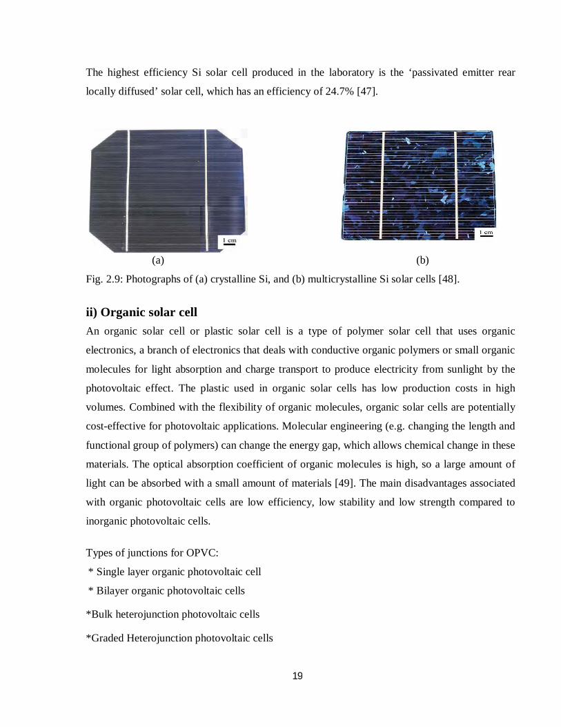
review the achievements of the different technologies. A photograph of a cell is given in Fig. 2.9.

(2.10)

19

The highest efficiency Si solar cell produced in the laboratory is the ‘passivated emitter rear

locally diffused’ solar cell, which has an efficiency of 24.7% [47].

(a) (b)

Fig. 2.9: Photographs of (a) crystalline Si, and (b) multicrystalline Si solar cells [48].

ii) Organic solar cell An organic solar cell or plastic solar cell is a type of polymer solar cell that uses organic

electronics, a branch of electronics that deals with conductive organic polymers or small organic

molecules for light absorption and charge transport to produce electricity from sunlight by the

photovoltaic effect. The plastic used in organic solar cells has low production costs in high

volumes. Combined with the flexibility of organic molecules, organic solar cells are potentially

cost-effective for photovoltaic applications. Molecular engineering (e.g. changing the length and

functional group of polymers) can change the energy gap, which allows chemical change in these

materials. The optical absorption coefficient of organic molecules is high, so a large amount of

light can be absorbed with a small amount of materials [49]. The main disadvantages associated

with organic photovoltaic cells are low efficiency, low stability and low strength compared to

inorganic photovoltaic cells.

Types of junctions for OPVC:

* Single layer organic photovoltaic cell

* Bilayer organic photovoltaic cells

*Bulk heterojunction photovoltaic cells

*Graded Heterojunction photovoltaic cells

20

The best efficiencies obtained with each cell type are given in Table 2.3 and the market share of

the different cell types during 2012 are given in Fig.2.10

Fig.2.10: Market share of solar cell types sold during 2012 [50].

Table 2.3 Best efficiencies reported for different solar cells and modules (Source: NREL, USA)[51]

Types of Solar Cell Efficiency (%) Silicon (Crystalline) 24.7 Silicon(Multicrystalline) 20.3 Silicon(thin film) 16.6 Silicon(amorphous) 9.5 Silicon(nanosrystalline) 10.1 III-V GaAs(Crystalline) 25.1 III-V GaAs(thin film) 24.5

III-V GaAs(Multicrystalline) 18.2

Thin film CIGS 18.4 Thin film CdTe 16.5 GaInP/GaAs/Ge 32.0 GaInP/GaAs 30.3 GaAs/CIS 25.8

21

Fig.2.11. Evolution of best laboratory efficiency for different solar cell technologies. (Source:

National Renewable Energy Laboratory, 2013) [52]

2.13 Module and Array The basic element of a PV System is the photovoltaic (PV) cell, also called a Solar Cell. An

individual silicon solar cell is quite small, typically about 6 inches square producing only about 1

or 2 watts of power.

To increase their utility, a number of individual PV cells are interconnected together in a sealed,

weatherproof package called a Panel (Module) [53].

To achieve the desired voltage and current, Modules are wired in series and parallel into what is

called a PV Array. The flexibility of the modular PV system allows designers to create solar

power systems that can meet a wide variety of electrical needs. Fig.2.12 shows PV cell, Panel

(Module) and Array.

22

Fig.2.12: PV cell, Module and Array [54]

In this way, solar systems can be built to meet almost any electric power requirement, small or

large. The picture in Fig. 2.13 below shows a small part of a Module with cells in it. It has a

glass front, a backing plate and a frame around it.

The performance of PV modules and arrays are generally rated according to their maximum

DC power output (watts) under Standard Test Conditions (STC). Standard Test Conditions are

defined by a module (cell) operating temperature of 25o C (77o F), and incident solar irradiance

level of 1000 W/m2 and under Air Mass 1.5 spectral distribution [55]. Since these conditions are

not always typical of how PV modules and arrays operate in the field, actual performance is

usually 85 to 90 percent of the STC rating.

Fig.2.13: Construction of a typical Mono-crystalline PV Solar Panel [56]

23

2.14 Review of Existing Models of PV Cell/Module Characteristics

The current-voltage (I-V) characteristic of a PV cell characterizes the non-linear electrical

behavior which strongly varies with sunlight intensity and the cell temperature. One-diode model

and the two-diode model are the two most commonly used PV cell equivalent circuits (Lasnier

and Ang, 1990). In this new era, there is a remarkable improvement in mathematical modeling

and simulation of photovoltaic modules. This section provides the related review of literatures on

the study performed by several researchers specifically in the mathematical modeling and

simulation of solar photovoltaic cells to predict system performance. Several models of PV

generator have been developed in literature [57-60]. The aim is to get the I-V characteristic in

order to analyze and evaluate the PV systems performance. The difference between all models is

the number of necessary parameters used in the computational. The most models used are:

•Single Exponential Ideal Diode Model without Any Resistance

• Explicit Model

• Solar Cell Model using Four Parameters

• Solar Cell Model using Five Parameters

• Solar Cell Model using Two Exponential

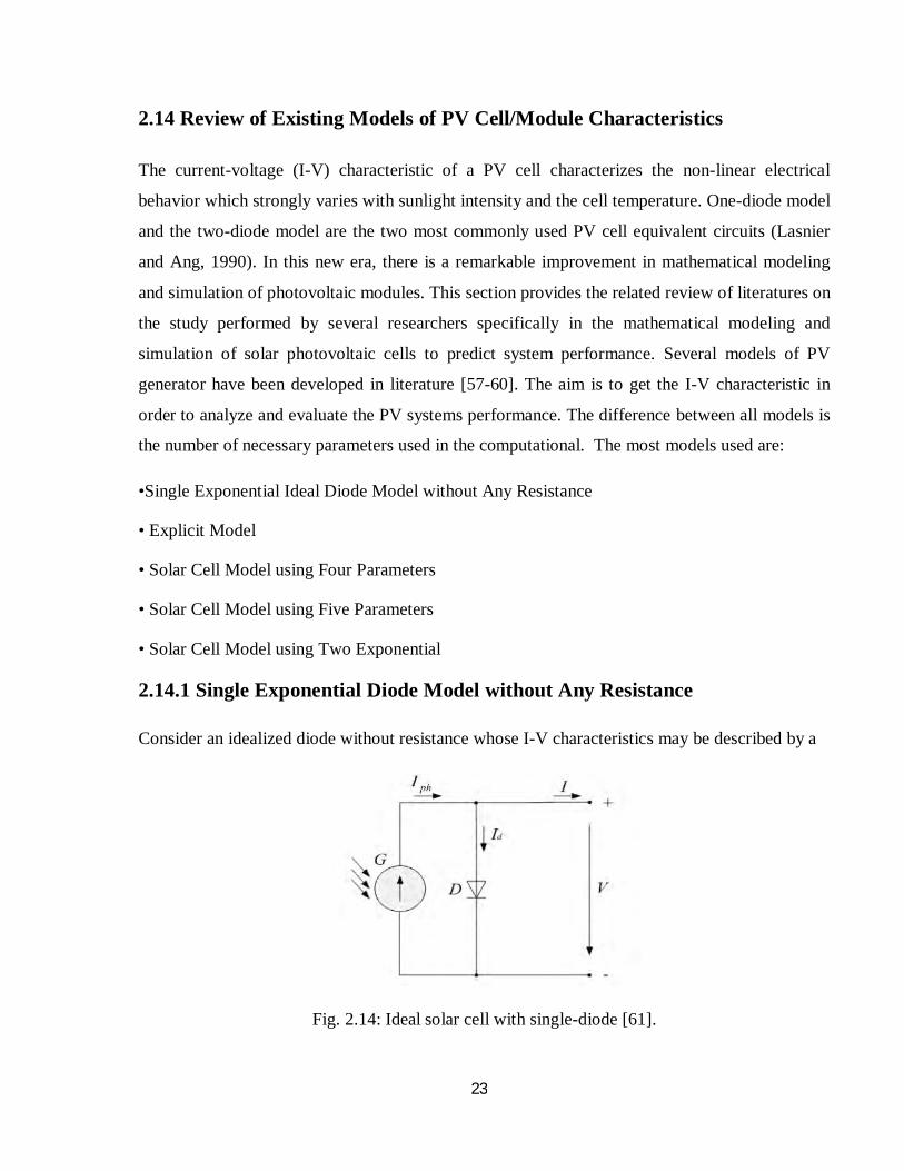
2.14.1 Single Exponential Diode Model without Any Resistance

Consider an idealized diode without resistance whose I-V characteristics may be described by a

Fig. 2.14: Ideal solar cell with single-diode [61].

24

lumped parameter equivalent circuit model consisting of a single exponential type ideal junction

[61].The terminal current I of this lumped equivalent circuit model is explicitly described in

mathematical terms by Shockley’s equation [62]:

The ideal equivalent circuit of a solar cell is a current source in parallel with a single-diode. The

configuration of the simulated ideal solar cell with single-diode is shown in Figure 1.

In Figure 1, G is the solar radiance, Iph is the photo generated current, Id is the diode current, I is

the output current, and V is the terminal voltage.

The I-V characteristics of the ideal solar cell with single diode are given by[64]:

Where,

I0 is the diode reverse bias saturation current,

q is the electron charge,

n is the diode ideality factor,

k is the Boltzman’s constant, and T is the cell temperature.

A solar cell can at least be characterised by the short circuit current Isc , the open circuit voltage

Voc , and the diode ideality factor n. For the same irradiance and p-n junction temperature

Conditions, the short circuit current Isc is the greatest value of the current generated by the cell.

The short current Isc is given by:

For the same irradiance and p-n junction temperature conditions, the open circuit voltage

(2.11)

(2.12)

25

Voc is the greatest value of the voltage at the cell terminals . The open circuit voltage

Voc is given by[65]:

The output power is given by:

Modeling for the single diode ideal model it has to consider ideal diode’s basic equation. For

Calculating the light generated current, block diagram seems like as shown in below.

Fig 2.15: Block diagram for calculate light generated current [66]

(2.13)

(2.14)

26

For calculating the Diode current, block diagram seems like as shown in below.

Fig. 2.16: Block diagram for calculate diode current [66]

Fig. 2.17: Block diagram for calculate current [66]

After calculate the current, we can easily find out the P (power). For that we have to just

multiplication the current with voltage.

27

Fig. 2.18: Current-Voltage characteristic of an ideal PV cell [66].

2.14.2 Explicit Model This model needs four input parameters, the short circuit current Isc , the open-circuit voltage

Voc, the maximum current Im, and the maximum voltage Vm [67]. The relation between the load

current I and the voltage V is given by [68]:

An explicit set of equations is written based on the ideal PV model given by Equation 2.15.A

single-diode without series and shunt resistances is considered, Equation 2.15 is used to write

down expressions for currents and voltages at each key point shown in Figure 2.14. Hence, the

short-circuit current, the open-circuit voltage, the maximum power voltage and current are

written as:

(2.15)

(2.16)

(2.17)

28

It is obvious that Equation 2.18 is implicit, therefore to obtain an explicit expression for every PV key

parameter this equation has to be rewritten in a different form. As has been previously mentioned, a PV

cell has a hybrid behavior, i.e., a current-source at the short-circuit point and voltage-source at the open-

circuit point. These two regions are characterized by two asymptotes of the I-V curve , where the

transition is a compromise between the two behaviors. It is interesting to remark that the maximum

power point corresponds to a trade-off condition where the current is still high enough before it starts

decreasing with increasing the output voltage. Based on this observation, the tangent of the I-V curve can

be used to evaluate the transition between current- to voltage-source controlled regions; this operation

yields:

This derivative is then used to calculate the output voltage that corresponds to the maximum

power operation condition of the cell; thus:

It is apparent that this equation requires an expression of the derivative of the current with

voltage evaluated at the maximum power point. The fact that the maximum power corresponds

to an extremum, the variation of the maximum output power with voltage is relatively small, i.e.,

a change on Vm has a relatively small effect on the maximum power of the cell. Therefore,

considering the asymptotic behavior of the I-V curve at short- and open-circuit conditions, the

derivative required by Eqn. 2.21 can be calculated as:

Replacing this equation into Equations 2.21 and 2.19, the voltage and current at the maximum

(2.18)

(2.19)

(2.20)

(2.21)

(2.22)

29

power point and consequently the maximum output power, are expressed as follows:

These equations are used to calculate key cell parameters at the maximum power point

as function of both cell temperature and irradiance, which are not necessarily given by PV

manufacturers. The following expression is used to calculate the photocurrent as function of

irradiance and temperature [67]:

where the reference state of the cell is given by the irradiance Gref = 1000 W/m2 and the

temperature Tref =298.15 K In this equation, µ1is a short-circuit current temperature coefficient

(A/K) and corresponds to the photocurrent obtained from a given PV cell working at (STC)

reference conditions (i.e., provided by cell manufacturers). Furthermore, Villalva et al. [68] have

proposed a relationship that allows the saturation current Io to be expressed as a function of the

cell temperature. In this work, this relation is explicitly written based on cell open-circuit

conditions using the short-circuit current temperature coefficient as well as the open-circuit

voltage temperature coefficient, hence [69]:

where Voc,ref is the reference open-circuit voltage and µv is an open-circuit voltage temperature

(2.23)

(2.24)

(2.25)

(2.26)

(2.27)

30

coefficient (V/K).Finally, the quality factor of the diode n, which is usually considered as a

constant [70], is determined at the reference state. Using the maximum power point current

equation and the saturation current at the reference temperature given by Eqn. 2.27, the diode

quality coefficient is determined as:

Where Vm,ref , Voc,ref , Im,ref and Isc,ref are key cell values obtained under both actual cell

temperature and solar irradiance conditions, usually provided by manufacturers.

The model is now completely determined; it requires the actual cell temperature, the actual Solar

irradiance and common data provided by manufacturers. The cell temperature, however, is

difficult to be established; applying the energy balance equation to a module at actual and NOCT

conditions, Duffie and Beckman [71] proposed a formulation for estimating the temperature as a

function of solar irradiance, and an overall convective and radiation heat transfer coefficient

from the cell to the environment. This coefficient is determined using a correlation that includes

the wind velocity.

Since this model is written based on the derivative of the I-V curve at the maximum power

operation point, the effect of this derivative is also investigated. Values obtained with the

proposed method are compared to real values also determined from the derivative of the I-V

curve at actual Vm and Im conditions by using the implicit set of equations. Further, a standard

mean error of 7.67 % is obtained between the derivative of the I-V curve at the maximum power

point for the present model and the similar one for the third reference case (i.e., the poorest

array). The characteristic I-V curves obtained by using iterative calculations as well as this

present model for the KC200GT array are plotted in Figures 2.19 to 2.22 [72]. The results for a

constant temperature of 25°C and for solar irradiances of 200 W/m² and 800 W/m² are shown in

Figures 2.19 and 2.21, respectively. Similar data obtained for a constant solar irradiance of 1000

W/m² and for cell temperatures of 10 and 50°C are illustrated in Figures 2.20 and 2.22,

respectively. From Figures 2.19 to 2.22, it is apparent that the temperature essentially affects

(2.28)

31

the voltage while the current seems to be mostly affected by the irradiance. It is obvious that for

high solar irradiances the proposed model is quite accurate. However, the open-circuit voltage at

low solar irradiance, as shown in Figures 2.19 and 2.21, is underestimated. In particular, the

temperature has a relative small effect on both the I-V and P-V characteristic key points of the

solar array, especially under short- and open-circuit conditions.

Fig. 2.19: Current-Voltage characteristics of the KC200GT array at T=25°C [72].

Fig. 2.20: Current-Voltage characteristics of the KC200GT array at G =1000 W/m² [72].

G=800 W/m2

G=200 W/m2

32

Fig. 2.21: Power-Voltage characteristics of the KC200GT array at T=25°C [72].

Fig. 2.22: Power-Voltage characteristics of the KC200GT array at G =1000 W/m² [72].

The model is based on an ideal cell where effects of series and parallel resistances are neglected.

This simplification allows an analytical method to be used for determining current, voltage and

power at every key operation conditions of the cell. Thus, explicit expressions are written for key

cell parameters without the necessity of performing iterative numerical calculations. Some

G=800 W/m2

G=200 W/m2

33

unknown parameters such as photocurrent, saturation current and diode quality factor are

calculated based on data usually provided by PV panel manufacturers. The proposed method is

validated against reference values obtained from iterative calculations applied to known solar

panels. The performance of the model is evaluated as a function of standard and weighted mean

errors observed between reference and estimated values. In general the proposed model is able to

provide quite accurate results; it is relatively simple to use and it can be very useful for design

engineers to quickly and accurately determine the performance of PV arrays as a function of

environmental constraints without carrying out numerical calculations.

2.14.3 Solar Cell Model Using Four Parameters More accuracy can be introduced to the model by adding a series resistance. The configuration

of the simulated solar cell with single-diode and series resistance is shown in Figure 2.23. The

classical equation describing the I-V curve of a single solar cell is given by [73]:

Fig. 2.23: Solar cell with single-diode and series resistance [73].

Where I is the load current and V the output voltage, I0 is the diode reverse saturation current ,

Iph is photo generated current, RS is the series resistance is the electric charge, K is the Boltzman

constant. T is the temperature (0K). The four parameters of this model are: Iph, I0, RS and n.The

effect of shunt resistance is not taking a count in this model. Equation (2.29) describes the I-V

curve quite well, but the parameters cannot be measured in a simple manner. Therefore, a fit

based on a smaller number of parameters which can be measured have been developed [74].

(2.29)

34

For the same irradiance and p-n junction temperature conditions, the inclusion of a series

resistance in the model implies the use of a recurrent equation to determine the output current in

function of the terminal voltage. A simple iterative technique initially tried only converged for

positive currents. The Newton–Raphson method converges more rapidly and for both positive

and negative currents [74].

The short circuit current Isc is given by [75]

Normally the series resistance is small and negligible. Hence, The open circuit voltage Voc is

given by:

The output power P is given by

The diode saturation current at the operating-cell temperature is given by:

Where I*0 is the diode saturation current at reference condition, TC is p-n junction cell

temperature, T* cell p-n junction at reference condition and ε is the band gap.

(2.30)

(2.31)

(2.32)

(2.33)

35

To simulate the selected PV array, a PV mathematical model having Np cells in parallel and Ns cells in series is used according to the following equation (neglecting shunt resistance):

Assuming that the selected solar module has Np equal to 1, the above equation can be

rewritten as:

The photo current, Iph , depends on the solar radiation (G) and the cell temperature (T)

according to the following equations as:

Where,

The series resistance of the cell is given as:

Where

The PV power, P, is then calculated as follows:

Using the above equations and the specifications supplied by the manufacturer data , a program

is developed using Matlab software to simulate the I-V and P-V characteristics of the 60W PV

panel as shown in Fig. 2.24 and Fig.2.25 respectively.

In Fig 2.24, the intersection of the graph with the y-axis gives the value of the short circuit

current of the solar cell, which in this case corresponds to 3.74 A. The open circuit voltage for

(2.34)

(2.35)

(2.36)

(2.37)

(2.38)

(2.39)

(2.40)

(2.41)

36

each cell is derived from the I-V plot. The crossing of the I-V curve with the voltage axis is the

open circuit voltage, which corresponds to almost 584 mV for each individual solar cell.

According to the specifications supplied in the Manufacturer Data Sheet (MDS) of the 60W

solar panel, there are 36 cells connected in series, hence the total open circuit voltage is 584mV

× 36 = 21.0V.

It is observed that the value of the open circuit voltage depends logarithmically on the Iph/Is

ratio. This implies that under constant temperature the value of the open circuit voltage scales

logarithmically with the short circuit current, but since the short circuit current scales linearly

with irradiance, the open circuit voltage is logarithmically dependent on the irradiance. This

relationship indicates that the effect of irradiance is much larger on the short circuit current than

that on the open circuit voltage value.

Fig. 2.24: Current-Voltage characteristics of 60W solar module [76]

A model of 60W solar panel is implemented in Matlab. The selected solar module represents 36

identical solar cells connected in series, with the same irradiance value. The I-V characteristic

of the solar module is expected to have the same short circuit current as a single solar cell while

the voltage drop is 36 times the voltage drop in one solar cell. The I-V characteristic of the solar

module is shown in Fig. 2.24.

37

Fig: 2.25: Power-Voltage characteristic of 60W solar module [76]

The output power of the solar cell is the product of the output current delivered to the load and

the voltage across the cell. The power at any point of the I-V characteristic is given by equation

2.41. There is no power output at the short circuit point where the voltage is zero and also at the

open circuit point where the current is zero. Power is generated between the short circuit point

and the open circuit point on the I-V characteristic. Somewhere on the characteristic, between the

two zero points, there exists a point where the solar cell generates the maximum power. The

point is called the maximum power point (MPP). A plot of the P-V characteristic of considered

solar module is shown in Fig 2.25.

The PV panel is modeled using the electrical characteristics of the solar panel provided by the

manufacturer’s data sheet. The open circuit voltage is 21.0V while the short circuit current is

3.74A. The maximum power delivered is 60W and the maximum power voltage and current

occur at 17.1V and 3.5A respectively. The PV module is initially modeled under varying

irradiation conditions with the solar cell temperature set to 25ºC. The I-V and P-V characteristics

of the solar panel for irradiance values of 200, 400, 600, 800, and 1000 W/m2 shown in Fig.2.26

and Fig. 2.27 respectively.

38

Fig. 2.26 Current-Voltage characteristics of 60W solar panel with varying irradiance [76]

Fig. 2.27: Power-Voltage characteristics of 60W solar panel with varying irradiance [76]

Operating temperature affects the electrical output of the solar module. The I-V and P-V

characteristics with varying operating temperatures are shown in Fig 2.28 and Fig 2.29

respectively. The module is set to operate with an irradiance value of 1000 W/ m2. The operating

temperatures are set at 25ºC, 40ºC, 50oC and 60ºC. The x-axis is the module’s voltage while the

y-axis is the module’s current or power.

39

Fig. 2.28: Current-Voltage characteristics of 60W solar panel with varying temperature [76]

Fig. 2.29: Power-Voltage characteristics of 60W panel with varying temperature [76] The short circuit current of the cell depends linearly on irradiation while the open circuit voltage

depends logarithmically on irradiation. Therefore it is observed that the output voltage should

increase as the irradiation level increases. However this is not necessarily so, since the cell

temperature is likely to rise as the irradiation level increases. An increase in cell temperature

will generally lead to a reduction of the output voltage. This makes it imperative to consider the

40

effect of temperature on the cell output voltage. Overall, there is a reduction of the voltage at

higher irradiances due to the accompanying higher cell temperature. A reduction in the terminal

voltage or current will lead to a decrease in the output power since both the voltage and current

are directly proportional to the output power, P = V * I.

2.14.4 Solar Cell Modeling Using Five Parameters:

Photovoltaic cell models have long been a source for the description of photovoltaic cell

behavior. The most common model used to predict energy production in photovoltaic cell

modeling is the single diode lumped circuit model [77]. In the single diode model, there is a

current source parallel to a diode. The current source represents light-generated current Iph that

varies linearly with solar irradiation. This is the simplest and most widely used model as it

offers a good compromise between simplicity and accuracy . Figure 2.30 shows the single diode

equivalent circuit model of PV cell which is commonly used in many studies and provides

sufficient accuracy for most applications.

In this model, the effect of shunt resistance is considered .Figure 2.30 shows a solar cell

equivalent circuit including series resistance Rs and shunt resistance Rsh [78].

Fig.2.30: Solar cell equivalent circuit including series resistance and shunt resistance

The mathematical description of this circuit is given by the following equation [79]:

The five parameters of this model are: Iph, I0, Rs, Rsh and n. For a given temperature and solar

irradiation intensity, these parameters are determined by using the open circuit voltage VOC, the

V

(2.42)

41

short circuit current Isc, the voltage Vm, and the current Im, at the maximum point and the slopes

of curve near VOC and ISC.

The light generated current of the module depends linearly on solar irradiation and is also

influenced by temperature [80] according to equation (2.43)

퐼ph = [퐼ph,n + 퐾I ∆푇 )]

The diode saturation current I0 dependance on temperature can be expressed by [81]

퐼0 = 퐼0,n n

푒푥푝 푞퐸G n

Where Eg is the band gap energy and I0,n the nominal saturation current at standard test

condition.

All model parameters can be determined by examining the manufacturer’s specification of

photovoltaic products. The performance characteristics of a PV module depend on its basic

materials, manufacturing technology and operating conditions. The most important points widely

used for describing the cell electrical performance are: the short circuit point where the current is

at maximum (short circuit current Isc) and the voltage over the module is zero; the open circuit

point where the current is zero and the voltage is at maximum (open circuit voltage Voc); the

Maximum power point where the product of current and voltage has its maximum. The power

delivered by a PV cell attains a maximum value at the points (Imp, Vmp).

Typically, three points (ISC, 0), (VOC, 0) and (Vmp, Imp) are provided by the manufacturer’s

datasheet at Standard Test Conditions. An accurate estimation of these points for other

conditions is the main goal of every modeling technique. From the aforementioned models, it is

obvious that the PV cell acts as a current-source near the short circuit point and as a voltage-

source in the vicinity of the open-circuit point. Therefore, the series resistance Rs, which

represents structural resistances of photovoltaic panel [81], has a strong effect in the voltage-

source region. In turn, the shunt resistance RSH that accounts for current leakage in [82] the p-n

junction, is of great importance in the current-source region and the maximum power point

(2.43)

(2.44)

42

appears to be compromise of the hybrid behavior of the cell between both voltage and current-

source region.

The values of the five parameters in the equation (2.42) must be determined to reproduce the I-V

curve of a PV system. This requires five equations containing five unknowns that should be

solved simultaneously to obtain the values of the parameters [83]. G .Walker [84] has further

simplified this model by removing the shunt resistance RSH to obtain a model as the four

parameters model. This model reliably predicts the performance of single crystal and

polycrystalline PV systems. The four parameters model assumes that the slope

of the I-V curve is flat at the short circuit condition.

For the five parameters model, the first equation is derived from open circuit condition where I

=0 and V = Voc. Equation (2.42) becomes

0 = 퐼ph – 퐼0 exp ( )

− 1 −

sh

The second equation occurs at short circuit condition where I = ISC and V =0. Then equation

(10) becomes

퐼 = 퐼ph – 퐼0 exp S

− 1 − S

sh

The measured current voltage pair at the maximum power point can be substituted into equation

(2.42) to obtain the third equation where I = Impp V=Vmpp

퐼 = 퐼ph – 퐼0 exp S

− 1 − S

sh

These three equations are obtained using the key points. In order to get another two equations,

we can differentiate equation (2.42) with respect to V; thus we get:

Again at the open circuit point on the I-V curve, V =Voc

and I = 0, therefore after substituting in equation (2.49) we obtain the following

results:

(2.46)

(2.45)

(2.47)

(2.48)

(2.49)

43

The power transferred from the P-V device at any point is given by:

An addition equation can be derived using the fact that on the P-V characteristic of a PV system

at the maximum power point, the derivative of power with voltage is zero.

After substituting in equation (2.49) the following equation is obtained:

The five parameters (Iph, I0, n, Rs and Rsh) can be obtained simultaneously solving these

equations in MATLAB using iterative method like Newton Raphson’s method to solve system of

nonlinear equations. For notational convenience, the following can be defined:

Based on the work [85], RS and Rsh can be obtained experimentally from the I-V curve. Thus the

initial can be calculated by calculating the diode ideality factor [86]:

(2.50)

(2.56)

(2.51)

(2.54)

(2.52)

(2.55)

(2.53)

44

The rest of the initial parameters can be found from the following equation

To compute the five parameter Iph, Io,Rs ,n and Rsh which are necessary to apply equation

(2.42), the above equations (2.54)-(2.57) have been used.

Finally, the equation of I-V characteristics is solved using the Newton Raphson’s method. In

order to validate the modeling and simulation method presented above for PV module, the

calculated values and experimental values are compared for a commercial polycrystalline silicon

cells from Solarex MSX60 module, composed of one parallel string of 36 solar cells.

The current for single diode with Rs and Rsh that diagram is look like as shown in below

Fig 2.31: Current block diagram for single diode with Rs and Rsh [87]

Fig.2.32: Current-Voltage characteristics at T=25 °C for various irradiance levels [87]

(2.57)

45

Fig.2.33: Power-Voltage characteristics at T=25 °C for different irradiances [87]

Fig.2.32 illustrates the dependence of I-V characteristics on temperature and irradiance for a

solarex MSX-60 module. The Fig.2.33 shows the P-V characteristics of the PV module with

varying irradiance at constant temperature. From the graph when the irradiance increases, the

output current and voltage also increases. This result shows the net increase in power output with

irradiance at constant temperatures. Also, in fig.2.34 and fig.2.35, the P-V and IV characteristics

Under constant irradiance (G=1000W/m2) with varying temperature are presented, respectively.

From these figures, when the operating temperature increases, the output current increases

dramatically while the output voltage decreases marginally, which results in a net reduction in

power with a rise in temperature.

Fig.2.34: Power-Voltage Characteristics at G=1000 W/m2 for various temperatures [87]

46

Fig.2.35: Current-Voltage characteristics at G=1000W/m2 for various temperatures

An accurate PV cell to module electrical model using five parameters is presented and calculated

using MATLAB software. The open circuit I-V and P-V curves, it is obtained from the

simulation of PV module designed in MATLAB environment explains in details its dependence

on the irradiation levels. These results obtained from the MATLAB model show excellent

correspondence to manufacturer’s published curves, the consistency between the data and found

the parameters given by manufacturers (Current, Voltage and Power).This paper provides a clear

and concise understanding of the I-V and P-V characteristics of PV module, which will serve as

the model for researchers in the field of PV modeling.

2.14.5 Solar cell Model Using Two Exponential

The accuracy of this model is more than the single diode model but there are some difficulties to

solve the equation. In this model, the solar cell is modeled as a current source connected in

parallel with a rectifying diode. However, in practice the current source is also shunted by

another diode that models the space charge recombination current and a shunt leakage resistor

to account for the partial short circuit current path near the cell’s edges due to the semiconductor

impurities and non-idealities. In addition, the solar cell metal contacts and the semiconductor

material bulk resistance are represented by a resistor connected in series with the cell shunt

elements [88]. The equivalent circuit for this model is shown in Fig. 2.36.

47

Fig 2.36: Solar cell equivalent circuit for model with two exponential [89].

In this double-diode model, the cell terminal current is calculated as follows:

where

IL: the terminal current,

Iph : the cell-generated photocurrent

I D1, I D2: the first and second diode currents,

Ish: the shunt resistor current.

The two diodes currents are expressed by Shockley equation as illustrated respectively in Eqs

(2.59) and (2.60), while the leakage resistor current Ish is formulated as shown in Eq.(2.61)

V

(2.58)

(2.59)

(2.60)

(2.61)

48

where Rs and Rsh are the series and shunt resistances respectively; ISD1 and ISD2 are the

diffusion and saturation currents respectively; VL is the terminal voltage; n1and n2 are the

diffusion and recombination diode ideality, K is is Boltzmann’s constant; q is the electronic

charge and T is the cell absolute temperature in Kelvin. Substituting Eqs. (2.59), (2.60) and

(2.61) into Eq.(2.58), the cell terminal current is now rewritten as shown in Eq. (2.62) [90].

The seven parameters to be estimated that fully describe the I-V characteristics Rs, Rsh, Iph, ISD1

and ISD2, n1 and n2.

Equations (2.62) is nonlinear transcendental functions that involve the overall output current

produced by the solar cell in both sides of the equation. Furthermore, the parameters Rs, Rsh,

Iph, Isd1, Isd2,n1 and n2 vary with temperature, irradiance and depend on manufacturing tolerance.

Such functions have no explicit analytical solutions for either IL or VL. various techniques such as

Numerical methods, curve fitting techniques, and different optimization methods are often

utilized to solve such functions. The PS optimization technique is employed to estimate the

parameters by minimizing a pre-selected objective function. In order to form the objective

function, the I-V relationships given in any of equations (2.62) is rewritten in the following

homogeneous equations:

The new objective function that sums the individual absolute errors (IAEs) for any given set of

measurements is defined as:

(2.62)

(2.63)

(2.64)

49

where N is the number of data points, ILi and VLi are ith measured current and voltage pair

values, respectively.

The currents Iph , Id1, Id2 and Ish can be implemented using Simulink blocks and are shown in

Fig.s (2.37), (2.38), (2.39). The estimated values of Rs and Rp are fed into the "From" blocks

along with the datasheet values and the constants. The value of the cell current "I" is fed from the

combined simulink block diagram shown in Fig.2.39. The iteration process starts by assuming

I=0 and continues until V becomes VOC. In a typical large PV power system, the cell modules

are in series-parallel combination (NS× NP, where NS, NP being the number of cells connected in

series and in parallel respectively). The output current equation then can be modified as:

Where Iph, Isd1, Isd2, Rsh, Rs, n1 and n2 are the individual cell parameters.

Fig 2.37: Simulink Block diagram for the Light-Generated Current, Iph [91].

(2.65)

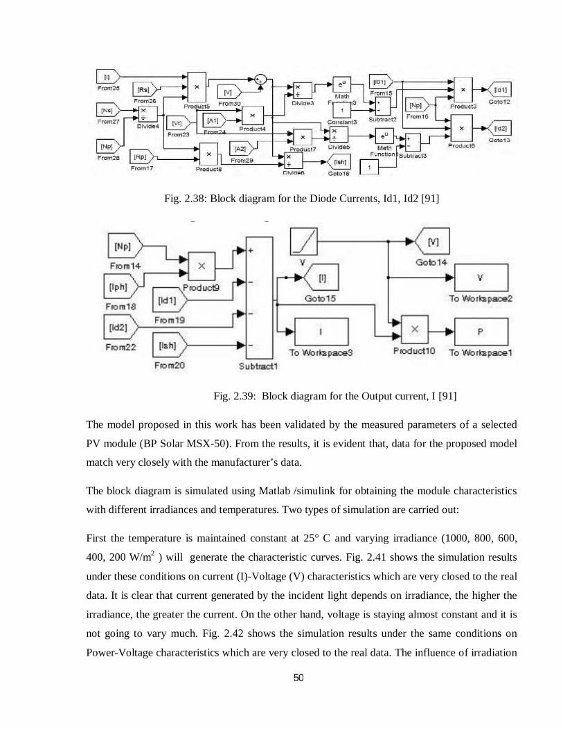
50

Fig. 2.38: Block diagram for the Diode Currents, Id1, Id2 [91]

Fig. 2.39: Block diagram for the Output current, I [91]

The model proposed in this work has been validated by the measured parameters of a selected

PV module (BP Solar MSX-50). From the results, it is evident that, data for the proposed model

match very closely with the manufacturer’s data.

The block diagram is simulated using Matlab /simulink for obtaining the module characteristics

with different irradiances and temperatures. Two types of simulation are carried out:

First the temperature is maintained constant at 25° C and varying irradiance (1000, 800, 600,

400, 200 W/m2 ) will generate the characteristic curves. Fig. 2.41 shows the simulation results

under these conditions on current (I)-Voltage (V) characteristics which are very closed to the real

data. It is clear that current generated by the incident light depends on irradiance, the higher the

irradiance, the greater the current. On the other hand, voltage is staying almost constant and it is

not going to vary much. Fig. 2.42 shows the simulation results under the same conditions on

Power-Voltage characteristics which are very closed to the real data. The influence of irradiation

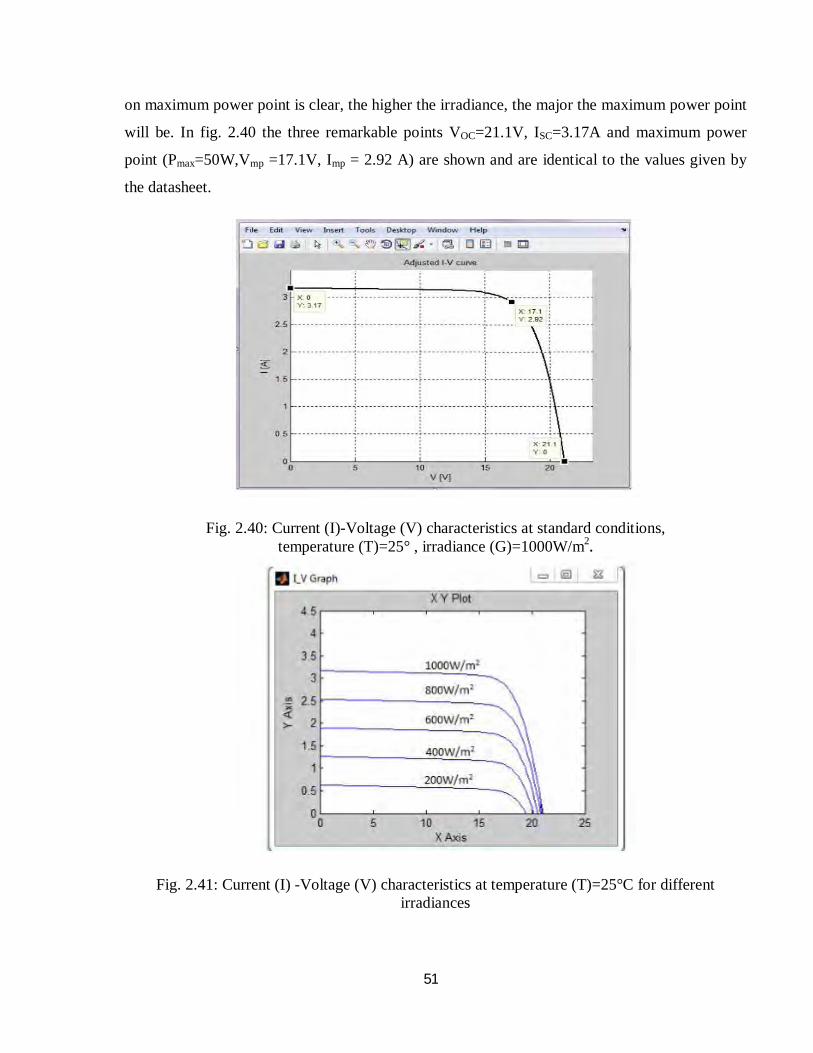
51

on maximum power point is clear, the higher the irradiance, the major the maximum power point

will be. In fig. 2.40 the three remarkable points VOC=21.1V, ISC=3.17A and maximum power

point (Pmax=50W,Vmp =17.1V, Imp = 2.92 A) are shown and are identical to the values given by

the datasheet.

Fig. 2.40: Current (I)-Voltage (V) characteristics at standard conditions, temperature (T)=25° , irradiance (G)=1000W/m2.

Fig. 2.41: Current (I) -Voltage (V) characteristics at temperature (T)=25°C for different irradiances

52

Fig. 2.42: Power (P)-Voltage (V) characteristics at temperature (T)=25°C with different irradiances.

Second the irradiance is maintained constant at 1000W/m2 and varying temperature (25° C, 50°

C, 75° C) will generate the characteristic curves. Fig. 2.43 show the simulation results of current

(I)-Voltage (V) characteristic under these conditions. The curves are very closed to the curves

given by data sheet. The current generated by the incident light is going to stay constant although

it increases slightly while the voltage decreases

Fig. 2.43: Current (I) –Voltage (V) characteristics at irradiance (G) =1000W/m2 for different temperatures.

53

Fig. 2.44 shows the simulation results under the same conditions on Power (P)-Voltage (V)

characteristics and is very closed to the real data. The effect of the temperature increase,

decreases voltage and power.

Fig. 2.44: Power (P) -Voltage (V) characteristics at irradiance (G) =1000W/m2 for different temperatures.

2.15: Limitation of Above Models:

The limitation of explicit model is that it doesn’t take account of series resistance Rs and shunt

Resistance Rsh. Four parameters model is based on single exponential model of solar cell and

and assume that Rsh is infinite, an assumption that may not be valid for the cell having low Rsh

values. The five parameters model is shown to give accurate reliable results but gives non

physical values at low illuminations [92].In actual silicon devices the recombination components

are a complex function of the carrier concentration. For example, in high efficiency PERL solar

cells as the number of carriers increase with the applied voltage, the recombination at the rear

surface changes dramatically with voltage. In such cases the analysis is best performed by a

single diode, but allowing both the ideality factor and the saturation current to vary with voltage

54

[93]. In such cases, which are quite common in silicon devices, a double diode fit yields

erroneous values. Maximum simulation model consider the fixed series resistance for all

illumination level. But practically it varies at different irradiation level. As a result Fill Factor

and efficiency also varies. This is the common limitation for modeling of solar cell.

2.16: Proposed Model for PV Module

Comparative study of various mathematical modeling of PV array has been done by different

researchers. Ideal single diode model (ISDM), Single diode model (SDM) and simplified single

diode model (SSDM) were utilized in order to carry on the comparative analysis [94] . Modeling

and simulation was done in Matlab/Simulink environment. Best model has been selected based

on the maximum power point (MPP) tracking and root mean square deviation (RMSD) from the

experimental data comparisons. Authors conclude that Single diode model with Rs and Rsh has

comparable accuracy levels. For this reason to overcome the limitations of above models,

proposed model is presented an experimental method for determination of Rs and Rsh of a solar

cell using the I-V characteristics based on Five Parameters model (Single diode model with Rs

and Rsh). It will be described elaborately in next chapter.

55

CHAPTER 3

Test System Modeling

3.1 Introduction This chapter presents the implementation of a generalized photovoltaic model using

Matlab/Simulink software package, which can be representative of PV cell, module, and array

for easy use on simulation platform. This makes the generalized PV model easily simulated and

analyzed in conjunction with power electronics for a maximum power point tracker. Taking the

effect of sunlight irradiance and cell temperature into consideration, the output current and power

characteristics of PV model are simulated and optimized using the proposed model. Several

methods are available in the literature for the measurement of series resistance and shunt

resistance [94-97].All these methods are based on single exponential model of solar cell and

assume that Rsh is infinite and presume Rs to be independent of the intensity of solar irradiance,

which may not be valid. In this work, it is proposed a new approach to simulate the I-V

characterization by series resistance to be dependent of the intensity of solar irradiance.

3.2 Photovoltaic Models Solar cell is basically a p-n junction fabricated in a thin wafer or layer of semiconductor. The

electromagnetic radiation of solar energy can be directly converted electricity through

photovoltaic effect. Being exposed to the sunlight, photons with energy greater than the band-

gap energy of the semiconductor are absorbed and create some electron-hole pairs proportional

to the incident irradiation. Under the influence of the internal electric fields of the p-n junction,

these carriers are swept apart and create a photocurrent which is directly proportional to solar

insolation. PV system naturally exhibits a nonlinear I-V and P-V characteristics which vary with

the radiant intensity and cell temperature. PV system naturally exhibits a nonlinear I-V and P-V

characteristics which vary with the radiant intensity and cell temperature. The typical I-V and P-

V characteristics of solar cell are shown in Fig. 3.1.

56

The fundamental parameters related to solar cell characteristics are Short circuit current (ISC),

Open circuit voltage (VOC), Maximum power point (MPP) and Fill factor.

Short Circuit Current is the current that corresponds to the short circuit condition when the

impedance is low and it is calculated when the voltage equals to zero. It is the greatest value of

the current generated by a cell. I (at V=0) = ISC.

Open Circuit Voltage is the voltage when the open circuit occurs and there is no current passing

through the cell. V (at I=0) = VOC.

Maximum Power Point is the operating point at which the power is maximum across the load. Pm

= Vm.Im, where Vm is the maximum voltage and Im is the maximum current.

Fill Factor (FF) is essentially a measure of quality of the solar cell. It is calculated by comparing

the maximum power to the theoretical power (Pm) that would be output at both the open circuit

voltage and short circuit current together. Fill Factor (FF) = Pm / (Voc.Isc). The fill factor is a

measure of the real I-V characteristic. Its value is higher than 0.7 for good cells. Typical fill

factors range from 0.5 to 0.82. Also the open circuit voltage (VOC) increases logarithmically with

the ambient irradiation, while the short circuit current (ISC) is a linear function of the ambient

irradiation.

Fig. 3.1 Typical Characteristics of solar cell [99]

57

3.3 PV Cell Model

A general mathematical description of I-V output characteristics for a PV cell has been studied

for over the past four decades. Such an equivalent circuit-based model is mainly used for the

MPPT technologies. The simplest equivalent circuit of the general model which consists of a

photo current, a diode, a parallel resistor expressing a leakage current, and a series resistor

describing an internal resistance to the current flow, is shown in Fig. 3.2 [100].

Fig. 3.2 PV Cell Equivalent Circuit Model.

The output of the current source is directly proportional to the light falling on the cell

(photocurrent IPH). During darkness, the solar cell is not an active device; it works as a diode, i.e.

a p-n junction. It produces neither a current nor a voltage. However, if it is connected to an

external supply (large Voltage) it generates a current ID, called diode current or dark current. The

diode determines the I-V characteristics of the cell.

The voltage-current characteristic equation of a ideal solar cell is given as [101]

퐼 = 퐼ph – 퐼d

퐼 = 퐼ph – 퐼0 exp ( ) − 1

The Equation (3.2) describing output current of the non-ideal practical PV cell was derived using

Kirchhoff’s current law as follows

퐼 = 퐼ph – 퐼d − 퐼sh

(3.2)

(3.1)

(3.3)

58

From Equation ( 3.3) ,we get the following equation

퐼 = 퐼ph – 퐼0 exp ( S)

− 1 − S

sh

Where

Iph is a light-generated current or photocurrent,

I0 is the reverse saturation current of diode (A),

q is the electron charge (1.602×10 -19 C),

V is the voltage across the diode (V),

K is the Boltzmann’s constant (1.381×10 -23 J/K),

TC is the junction temperature in Kelvin (0K).

n Ideality factor of the diode

RS is the series resistance of diode,

Rsh is the shunt resistance of diode

The complete behavior of PV cells is described by five model parameters (Iph, n, Is, Rs, Rsh)

which is representative of the physical behavior of PV cell/module. These five parameters of PV

cell/module are in fact related to two environmental conditions of solar irradiance & temperature.

The determination of these model parameters is not straightforward owing to non-linear nature of

equation (3.4). Based on equation 3.4, the Matlab/SIMULINK model was developed.

The above model includes two subsystems: one that calculates the PV cell photocurrent mainly

depends on the solar irradiance and cell’s working temperature, which is described as [102]

퐼ph = [퐼SC + 퐾I (푇C − 푇Ref )]

Where

ISC is the cell’s short-circuit current at a 25°C and 1000W/m2,

KI is the cell’s short-circuit current temperature coefficient,

TRef is the cell’s reference temperature,

and G is the solar irradiance in W/m2.

An approximate expression for calculating the cell temperature is given by [103]:

(3.4)

(3.5)

59

푇 = 푇 + 퐺

Where,

The best module operated at a NOCT of 33°C, the worst at 58°C and the typical module at 48°C respectively.

G= Irradiance in W/m2.

On the other hand, the cell’s saturation current varies with the cell temperature, which is described as [5]

퐼0 = 퐼RS 푇C

푇Ref

3 푒푥푝 푞퐸G

1푇Ref− 1푇C

푘푛

Where

IRS is the cell’s reverse saturation current at a reference temperature and a solar radiation,

EG is the bang-gap energy of the semiconductor used in the cell.

n is the ideal factor dependent on PV technology and is listed in Table 3.1 [104].

TABLE 3.1 Ideality factor n dependence on PV technology

The reverse saturation current at reference temperature can be approximately obtained as [105]: 퐼RS = SC

OC

S C

Where VOC is the PV open-circuit voltage at the reference temperature

The double exponential model is another more accurate model that describes the PV cell [106].

This model consists of a light-generated current source, two diodes, a series resistance and a

parallel resistance. However, because implicit and nonlinear nature of the model is difficult to

Technology Ideal Factor (n) Si-Mono 1.2 Si-Poly 1.3 a-si:H 1.8 a-Si:H tandom 3.3 a-Si:H triple 5 Cd Te 1.5 CIS 1.5 AsGa 1.3

(3.6)

(3.7)

(3.8)

60

develop expressions for the I-V curve parameters, therefore, this model is not widely used in

literature and is not taken into consideration for the generalized PV model.

The approximate model of a PV cell with suitable complexity can be derived from Eq. (3.4) via

neglecting the effect of the shunt resistance and be rewritten as :

퐼 = 퐼ph – 퐼o exp ( S)

C− 1

For an ideal PV cell (no series loss and no leakage to ground, i.e., RS = 0 and RSH = ∞,

respectively). The equivalent circuit of PV cell can be further simplified where Eq. (1) can be

rewritten as[12]:

퐼 = 퐼ph – 퐼0 exp ( )

− 1

When I=0, then the output voltage is termed as the open circuit voltage Voc,

shown as in Eq.( 3.11).

푉 = 푙푛 + 1

3.4 PV Module and Array Model

Since a typical PV cell produces less than 2W at 0.5V approximately, the cells must be

connected in series parallel Configuration on a module to produce enough high power. A PV

array is a group of several PV modules which are electrically connected in series and parallel

circuits to generate the required current and voltage. The equivalent circuit for the solar module

arranged in NP parallel and NS series is shown in Fig. 3.3(a). The terminal equation for the

current and voltage of the array becomes as follows [107].

퐼 = 푁P퐼ph − 푁P퐼0 exp푞 푉푁S

+ 퐼푅S푁P

푛푘푇C

− 1 −푁P푉푁S

+ 퐼푅S 푅sh

An approximate equivalent circuit for PV cell, module, and array can be generalized and

expressed in Fig. 3.3(b). Therefore, the current can be expressed as

(3.9)

(3.10)

(3.12)

(3.11)

61

퐼 = 푁P 퐼ph − 푁P 퐼0 exp푞 푉푁S

+ 퐼푅S푁P

푛푘푇 − 1

(a) Generalized array model

(b) Approximate array model

(c) Simplified array model

Fig. 3.3 Equivalent circuit models of generalized PV array.

(3.13)

푵푺

푵푷푹푺

푵푺

푵푷푹푺푯

… …푵푷. . …푵푺

푵푺푰푷푯 I

V

푵푺푰푷푯

푵푺

푵푷푹푺

IV푵푺 …푵푷. . …

푵푺푰푷푯

…푵푷.푵푺 V

I

62

Where NS = NP = 1 for a PV cell, NS and NP are the series-parallel number for a PV array. The

simplified model of a generalized PV array is illustrated in Fig. 3.3(c). The equivalent circuit is

described as:

퐼 = 푁P 퐼ph − 푁P 퐼0 exp푞

푁S 푛푘푇− 1

Where Total shunt Resistance;

푅 = 푅sh sp

Total series Resistance:

R = 푅 NNp

3.5 Newton Raphson Algorithm

In this project, the generalized PV module and array models have been used for the PV modeling

using Matlab/Simulink. The output current is required to be an input to the equations of output

current in this model. Iterations may be needed for solving this problem which in many cases end

up with simulation break. Newton Raphson method is used for finding the root of a non linear

function by successively better approximation. If f(x) is a non linear function the first step is to

find the derivative f’(x). Next step is choosing an initial x value xn. Each successive value of x

closer to the value of x for f(x)=0,can be calculated by Eqn.3.17 [108]

Here the value current instead of x.Then the Eqn.(3.12) become

퐼푛 + 1 = 퐼푛 − ( )´( )

Then function of current can be expressed as

푓(퐼) = 퐼 1 +푅푅 − 푁 퐼 + 푁 퐼 exp

푞 푉푁 + 퐼푅

푛퐾푇 − 1 +

푉푁푅

The derivative of f(I) is equal to

푓´(퐼) = (1 +푅푠푇푅푠ℎ푇 –푁푝

푞푅푠푇퐴퐾푇푐 퐼표 exp

푞 푉푁푠 + 퐼푅푠푇푛퐾푇푐

When V=0 ,I=Isc .So we can start with the initial value I=Isc .

(3.17)

(3.18)

(3.19)

(3.15)

(3.16)

(3.14)

63

3.6 Simulation Tools As shown in Fig. 3.4, using Simulink math operations toolbox and Sim Power Systems toolbox,

the simplified model of the PV cell has been simulated using math function block for the

equations of the PV simplified model. The inputs and the parameters are the same as in the

physical model with additional parameters such as, the quality factor, semi-conductor band-gap

energy, and number of cells in series and parallel. A short description of these tools has been

given below. The mathematical PV cell model that is illustrated in Fig. 3.4 has been used as a

sub-system to be integrated into other system simulation and provide an easy way to input the

parameters of the PV module. The mathematical model has more advantages than the physical

model, because additional parameters as quality factor and semi-conductor band gap energy can

be varied/controlled. Moreover, parallel and series PV cells combinations can be formed without

the need for repeating the block diagrams. On the other hand and in order to make a parallel

combination in the physical model, the block of the PV cell has to be duplicated, which add more

complexity to the model. Since Simulink has a powerful toolbox for modeling the power systems

and power electronics components, it is important to illustrate how to interface the mathematical

PV model with the power system toolbox.

3.7 PV Module Simulation at Standard Condition

The PV module simulation on Simulink is shown in Fig.3.4 .The model comprise two graph of

Power-Voltage and Current-Voltage. The input to the simulation is given from the manufactures

datasheets. The other simulation parameters are set in the following values: TC= 25 Degree

Celsius, n=1.3(Polycrystalline solar cell), Rsh=50KΩ, Rs=5mΩ. This value can be varied as any

required. The simulation is done in standard condition to verify the working of simulink PV

model. The unknown parameters are calculated and power voltage and current voltage

characteristics are simulated. The unknown parameters are saturation current at reference

temperature ISR, saturation current Io and Short circuit current ISC at the given temperature are

calculated from the input parameters. We can enter the atmospheric temperature, the system

calculate the cell temperature TC. Series Resistance is found from the developed sub system of

this model. From the input parameters and calculated unknown parameters the simulating

system draw the current voltage, Power voltage and Maximum power point tracking graph.

64

Fig. 3.4 simulation models of generalized PV array.

Fig 3.4: Simulation model of generalized PV array

65

CHAPTER 4

Experimental and Simulation Results Analyses

4.1 Introduction Simulation results of different analyses performed on the proposed model of solar cell as

developed in chapter-4, are presented in this chapter. In this analysis the effect of irradiation and

atmospheric temperature on current -voltage characteristics and power- voltage characteristics

are studied. In this chapter authors also try to show that parasitic resistance of the solar cell be a

function of irradiance that was not considered in any PV model. All effects are observed from

105 W/m2 to 602 W/m2 in this experiment. But simulation is done up to 1000 W/m2.

4.2 Experimental Setup

Fig. 4.1: Schematic diagram of a solar cell/module measurement system.

In this study, the block diagram of the experimental set up is shown in Fig. 4.1. It consists of a

rheostat, a Pyranometer to measure the solar Irradiance, two digital multi-meters and a solar

panel that has the key specifications listed in Table 4.1.

V

Solar cell/module

A

Potentiometer

Pyranometer

66

Table 4.1: Major Specifications for the test module

Shinew XH SERIES,Model:XH-36M-5 Maximum Power (Pmax) 5 W Open Circuit Voltage (Voc) 21.47 V Short Circuit Current (Isc) 310m A Voltage at Pmax 17.40 V Current at Pmax 290 mA Module Dimensions 342×160×25 mm Module Weight 0.8kg Cell Type Mono crystalline No. of cells 36 in series Data measured in standard condition(STC): Irradiation 1000 W/m2, AM1.5, cell temperature 250C,Tested according to: IEC 61215 and IEC 61730

4.3 Experimental Result The term Irradiance is defined as the measure of power density of sunlight received at a location

on the earth and is measured in watt per meter square. Whereas irradiation is the measure of

energy density of sunlight. The term Irradiance and Irradiation are related to solar components.

As the solar Irradiation keeps on changing throughout the day similarity I-V and P-V

characteristics varies with the increasing solar irradiance both the open circuit voltage and the

short circuit current increases and hence the maximum power point varies which shows in Fig.

4.2 and Fig. 4.3 .In Fig. 4.2 shows the I-V characteristics at six different irradiation levels. It is

observed that the value ISC which is minimum (0.03A) at irradiation, 105 W/m2 and it is

maximum (0.19A) at irradiation, 602 W/m2.

Fig. 4.2: Current- voltage characteristics at six various irradiance levels.

0.00

0.05

0.10

0.15

0.20

0.00 5.00 10.00 15.00 20.00 25.00

Irradiance 105 W/m^2Irradiance 202 W/m^2Irradiance 304 W/m^2Irradiance 400 W/m^2Irradiance 502 W/m^2Irradiance 602 W/m^2

Cur

rent

(A)

Voltage(V)

67

It is observed that the value ISC which is minimum (0.03A) at irradiation, 105 W/m2 and it is

maximum (0.19A) at irradiation, 602 W/m2.

Fig.4.3 : Power Voltage characteristics at six different irradiance levels

In Fig. 4.3 shows the P-V characteristics at six different irradiance levels. It is

observed that the value Pmax which is minimum (0.226 W) at irradiation, 105 W/m2

and it is maximum (2.6 W) at irradiation, 602 W/m2.

Fig. 4.4(a): Short circuit current as a function of Irradiance (Experimental data in this work.)

0.00

0.50

1.00

1.50

2.00

2.50

3.00

0.00 5.00 10.00 15.00 20.00 25.00

105 W/m^2202 W/m^2304 W/m^2400 W/m^2502 W/m^2602 W/m^2Po

wer

(W)

Voltage (V)

0

0.05

0.1

0.15

0.2

0.25

0 100 200 300 400 500 600 700

Shor

tcir

cuit

curr

ent (

Isc)

,(A)

Irradiance (W/m2)

68

Fig. 4.4(b): Short circuit current as a function of Irradiance

(Another experimental data) [109] The PV cell current is strongly dependent on the solar Irradiance. However, the voltage has a

small change with increasing intensity of solar irradiance. The effect of irradiance on open

circuit voltage (VOC) and short circuit current (ISC) have described in Fig. 4.4 and Fig. 4.5. Short

circuit current (ISC) is proportionally increasing with increasing irradiance. But the change of

VOC is very small with increasing irradiance.

Fig. 4.5(a): Open circuit votage as a function of Irradiane

(Experimental data in this work.)

0

0.5

1

1.5

2

2.5

3

3.5

0 200 400 600 800 1000 1200

Shor

tcir

cuit

curr

ent

(Isc)

(A)

Radiation(W/m2)

02468

101214161820

0 100 200 300 400 500 600 700

open

cir

cuit

vota

ge(V

oc)

Irradiance (W/m2)

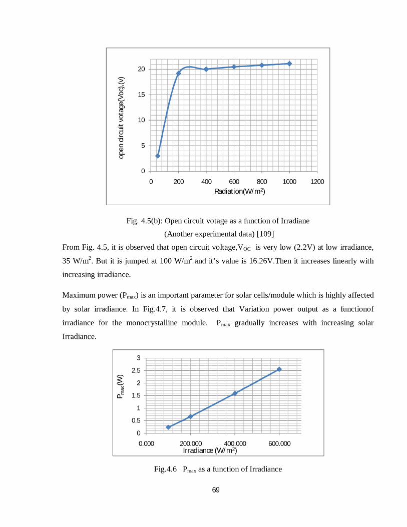
69

Fig. 4.5(b): Open circuit votage as a function of Irradiane (Another experimental data) [109]

From Fig. 4.5, it is observed that open circuit voltage,VOC is very low (2.2V) at low irradiance,

35 W/m2. But it is jumped at 100 W/m2 and it’s value is 16.26V.Then it increases linearly with

increasing irradiance.

Maximum power (Pmax) is an important parameter for solar cells/module which is highly affected

by solar irradiance. In Fig.4.7, it is observed that Variation power output as a functionof

irradiance for the monocrystalline module. Pmax gradually increases with increasing solar

Irradiance.

Fig.4.6 Pmax as a function of Irradiance

0

5

10

15

20

0 200 400 600 800 1000 1200

open

cir

cuit

vota

ge(V

oc),(

v)

Radiation(W/m2)

0

0.5

1

1.5

2

2.5

3

0.000 200.000 400.000 600.000Irradiance (W/m2)

P max

(W)

70

The fill factor is denoted as FF, is a parameter that helps in characterizing the non-linear

electrical nature of the solar cell. Fill factor is defined as the ratio of the maximum power from

the solar cell to the product of VOC and ISC and it gives an idea about the power that a cell can

produce with an optimal load under given conditions, P=FF*Voc*Isc. Fill factor is also an

indicator of quality of cell. With FF approaching towards unity the quality of cell gets better. Fill

Factor can be improved in many ways. In Fig. 4.7 shows the variation of fill factor with changing

Irradiance. It is observed that fill factor is gradually rising with increasing irradiance. It is

maximum (0.74) at Irradiance, 602 W/m2.

Fig. 4.7 Fill Factor as a function of Irradiance

The efficiency is the most commonly used parameter to compare the performance of one solar

cell to another. Efficiency is defined as the ratio of energy output from the solar cell to input

energy from the sun. In addition to reflecting the performance of the solar cell itself, the

efficiency depends on the spectrum and intensity of the incident sunlight and the temperature of

the solar cell. Therefore, conditions under which efficiency is measured must be carefully

controlled in order to compare the performance of one device to another. In Fig. 4.8, It is

described that how efficiency varying with varying radiation variation.

0.4

0.45

0.5

0.55

0.6

0.65

0.7

0.75

0.8

0.000 200.000 400.000 600.000Irradiance(W/m2)

Fill

Fact

or

71

Fig. 4.8: Efficiency as a function of Irradiance

It is observed that efficiency is rising up with solar irradiation. It is maximum (13.6%) at radiation, 602 W/m2.

Resistive effects in solar cells reduce the efficiency of the solar cell by dissipating power in the

resistances. The most common parasitic resistances are series resistance and shunt resistance. In

most cases and for typical values of shunt and series resistance, the key impact of parasitic

resistance is to reduce the fill factor. Both the magnitude and impact of series and shunt

resistance depend on the geometry of the solar cell, at the operating point of the solar cell. Series

resistance in a solar cell has three causes: firstly, the movement of current through the emitter

and base of the solar cell; secondly, the contact resistance between the metal contact and the

silicon; and finally the resistance of the top and rear metal contacts. The main impact of series

resistance is to reduce the fill factor, although excessively high values may also reduce the short-

circuit current. Practically Series resistance is highly affected by irradiance but no model

consider this effect. In Fig.4.9, the effect of irradiance on series resistance is shown. The raise of

the series resistance is rapid for small illumination levels. This resistance varies from 128.15

ohms to 14.35 ohms between 105 W/m2 to 602 W/m2. As pointed out, the decrease can be

attributed it to the increase in conductivity of the active layer with the increase in the intensity of

irradiance.

5

6

7

8

9

10

11

12

13

14

15

0.000 200.000 400.000 600.000Radiation (W/m2)

Effic

ienc

y (%

)

72

Fig.4.9: Series resistances as a function of Solar Irradiance

In Fig. 4.10, It is described that how efficiency varying with varying Series Resistance of the

solar cell. It is observed that efficiency is rising up with decreasing series resistance. Efficiency

varies from 7.7% to 13.6% between 128.15 ohms to 14.35 ohms.

Fig.4.10: Efficiency as a function Series Resistance

Significant power losses caused by the presence of a shunt resistance, RSH, are typically due to

manufacturing defects, rather than poor solar cell design. Low shunt resistance causes power

losses in solar cells by providing an alternate current path for the light-generated current. Such a

diversion reduces the amount of current flowing through the solar cell junction and reduces the

voltage from the solar cell. The effect of a shunt resistance is particularly severe at low light

levels, since there will be less light-generated current. The loss of this current to the shunt

therefore has a larger impact. An estimate for the value of the shunt resistance of a solar cell can

be determined from the slope of the I-V curve near the short- circuit current point. In addition, at

0.00

20.00

40.00

60.00

80.00

100.00

120.00

140.00

0.00 200.00 400.00 600.00

Irradiance (W/m2)

Seri

esRe

sist

ance

(Rs)

,Ω

56789

101112131415

10.00 30.00 50.00 70.00 90.00 110.00 130.00Series Resistance,Rs (Ohms)

Effic

ienc

y (%

)

73

lower voltages where the effective resistance of the solar cell is high, the impact of a resistance

in parallel is large. In Fig.4.11, the effect of irradiance on shunt resistance is shown in below.

The shunt resistance shows a marked dependence on the irradiance in this curve. It is observed

from this curve, RSH decreases with increasing irradiance. The change of shunt resistance, RSH is

not large. It is varied from 1071.2 ohms to 1070.13 between 105 W/m2 to 602 W/m2.

Fig. 4.11: Shunt resistance as a function of Solar Irradiance It is possible to approximate the series and shunt resistances, Rs and Rsh, from the slopes of the I-

V curve at VOC and ISC, respectively. The resistance at Voc, however, is at best proportional to

the series resistance but it is larger than the series resistance. Rsh is represented by the slope at

ISC. Typically, the resistances at ISC and at VOC will be measured and noted, as shown in Figure

4.12.

.

Fig.4.12 : Obtaining Resistances from the I-V Curve

1065.001066.00

1067.001068.00

1069.001070.00

1071.001072.00

1073.001074.00

1075.00

0.00 200.00 400.00 600.00Irradiance (w/m2)

Shun

tRe

sist

ance

(Rsh

),Ω

74

Where

푅 = 푉 퐼

푅 = 푉 퐼

From Fig 4.2, it is found the value of Rs and Rsh by using method that is described in fig 4.12. In

table 4.2, it is shown that the value of series and shunt resistance is varying with Solar irradiance

variation.

Table 4.2: Datasheet of Series and Shunt Resistance w.r.t Solar Irradiance

Solar Irradiation(W/m2) 100.00 200.00 300.00 400.00 500.00 600.00 Rs (Ω) 128.15 39.41 30.60 22.69 16.17 14.35 Rsh (Ω) 1071.20 1070.79 1070.79 1070.57 1070.36 1070.13

The author has developed an empirical equation for the irradiance effect on series resistance of

solar cell by using experimental data.

푅 (푚푒푎푠푢푟푒푑) = 푅 (푟푒푓) 푘1푒푥푝 푘2

퐺sinh(푘3 × 퐺)

Where Rs(ref)=Value of series resistance at reference irradiation 1000 w/m2

k1, k2 and k3 are constant [k1=1.5714, k2=27 and k3=0.001255] G=measured solar irradiance

The experimental series resistance value and equation series resistance value are shown in table

4.3. Based on the above equation, the subsystem of Fig. 4.13 is obtained.

Fig. 4.13: Rs Matlab/SIMULINK subsystem for varying solar Irradiance.

(4.1)

75

Table 4.3: Compare series resistance between experimental and developed equation value

Solar Irradiance (W/m2) 100.00 200.00 300.00 400.00 500.00 600.00 RS (Ohms) (Experimental value) 116.25 46.41 30.60 22.69 16.17 14.35 RS (ohms) (Equation value) 114.47 49.62 31.21 22.48 17.33 13.92 Deviation error(%) 1.53% 6.91% 1.99% 0.92% 7.17% 2.99% The author could not able to measure the series resistance over 600 W/m2 due to weather

condition of Bangladesh. But it is possible by using the equation which is shown fig 4.14. From

the figure, it is shown that both results are approximately same for all irradiance levels.

Fig 4.14: Series resistance as a function of solar Irradiance

(Compare between experimental and equation value)

This equation is compared with another experimental data [108] .It is shown in table 4.4. Table 4.4: Compare equation with another experimental data

Solar Irradiance (W/m2)

100 200 300 400 500 600 700 800 900 1000

RS (Ohms) (Experimental value) 1.40 0.71 0.52 0.32 0.26 0.22 0.19 0.14 0.11 0.11

RS(ohms) (Equation value) 1.45 0.72 0.47 0.35 0.27 0.22 0.18 0.15 0.13 0.11

0.00

20.00

40.00

60.00

80.00

100.00

120.00

140.00

0 200 400 600 800 1000 1200Irradiance (W/m2)

Seri

esRe

sist

ance

(Rs),Ω

76

Fig 4.15: Series resistance as a function of solar Irradiance

(Compare between another experimental data and equation value)

From Fig 4.15, it shown that developed equation is valid for another experimental data.

Figure 4.16 illustrates the effect of solar intensity on ideality factor of crystalline solar cell. It is

observed that ideality factor decreases with increasing solar Irradiance. It varies from 2.5 to 1.2

with varying 101 W/m2 to 602 W/m2. The value of n is extracted by using equation (4.2) [109].

In a silicon solar cell, the values of n are governed by the combination of space charge

recombination, bulk recombination and surface recombination mechanisms. The space charge

recombination is more effective at low intensities and low junction voltage. So the higher n

values at lower intensities as shown in fig 4.16 can be attributed to the larger contribution of

space charge recombination to the total recombination in the cell. The contribution of space

recombination decreases at higher Irradiance and then, the values of n also decrease with

increasing solar irradiance.

0.00

0.20

0.40

0.60

0.80

1.00

1.20

1.40

1.60

0 200 400 600 800 1000 1200

experimental data

equation value

Irradiance (W/m2)

Seri

esRe

sist

ance

(Rs)

,Ω

(4.2)

77

Fig 4.16: Ideality factor (n) as a function of solar Irradiance

4.4 Comparing Efficiency between Monocrystalline and Polycrystalline Solar Module: An experiment to investigate the performance of two photovoltaic modules is conducted at

different times of the day. The relationship between the performance and the efficiency of mono

crystalline PV and multi crystalline PV is measured in this experiment. The performance value

of the PV solar module is identified and compared with the output values supplied by the

producer of the PV modules and with other PV modules. The experimental investigation has

been carried out at the venue of the BUET. Measurements were taken from the two PV modules.

Efficiency of each panel under the recorded conditions was calculated. Input power has been

calculated by multiplying the incident solar radiation with the PV area. Output power has been

calculated using measured values of the generated voltage and current. Efficiency variation

accordance to solar radiation and output conditions has been calculated and presented in this

section. The panels that have been used in the experimental work and their specifications are

presented in Table 4.5

0.000

0.500

1.000

1.500

2.000

2.500

3.000

0 200 400 600

Irradiance(W/m2)

Idea

lity

Fact

or,n

78

Table 4.5: Specifications of PV panels used in this experiment

PV SOLAR PANEL MODEL

XH-36M-5 ROS05-36M

Maximum power (Pmax) 5 W 5 W Open circuit Voltage (VOC) 21.47V 21.5V Short circuit current (ISC) 310mA 320mA Voltage at Pmax 17.40 V 17.40 V Current at Pmax 290 mA 290 mA Module dimensions 342×160×25mm 300×217×28mm Module weight 0.8kg 0.9kg Cell type Mono crystalline Poly crystalline No. of cells 36 in series 36 in series Data measured in standard condition(STC):Irradiation 1000 W/m2, AM1.5,cell temperature 250C,Tested according to: IEC 61215 and IEC 61730

At early morning solar radiation has a low angle and solar rays penetrate a thick atmospheric

layer. Abundance in radiation occurs at noon, when sun is at the highest angle above the horizon

and radiation encounters minimum thickness of the atmosphere.

The highest radiation intensity was obtained at mid day when sun ray is perpendicular on the

surface. The recorded values are in the range 438 W/m2 in the morning and 463 W/m2 in the

afternoon and 570 W/m2 at midday. The variation in radiation intensity caused variation in the

measured output current which affects efficiency in the same manner. Fig. 4.17 shows solar

Irradiance measurement per hour in randomly.

Output current and voltage of each panel was measured every hour in a randomly selected day

under similar conditions. The open circuit voltage and short circuit current has been measured

directly from the PV panels output without battery connection or electrical load. The efficiency

curve of mono crystalline and multi crystalline PV panels is plotted.

However, the ambient temperature has a considerable effect on the efficiency of PV system. As

the ambient temperature increases cell temperature increases, the open circuit voltage decreases

and the short circuit current become slightly higher to reach the maximum output current. In the

present investigations, the measurements for both types of PV panels have been carried out at the

same time which means that the ambient temperature and temperature of the PV panels were

79

identical. Therefore, the influence of ambient temperature on the efficiency of PV panels is

abandon.

Fig 4.17: Irradiance as a function of time in a day (city :Dhaka,date:19/07/2013)

Fig 4.18:Pmax as a function of time in a day (city :Dhaka,date:19/07/2013)

0

100

200

300

400

500

600

Irra

dian

ce ,W

/m2

Time,hr

0

0.5

1

1.5

2

2.5

3

7 8 9 10 11 12 13 14 15 16 17 18

mono

poly

Pmax

,W

Time,Hr

80

Fig 4.19: Efficiency as a function of time in a day (city :Dhaka,date:19/07/2013)

Figure 4.19 illustrates the efficiency curves for both mono crystalline and multi crystalline PV

cells. Figure 4.19 indicates that mono crystalline PV cells have higher efficiency value than multi

crystalline PV cells. The efficiency of mono crystalline PV cells can reach 15.27% while

efficiency of multi -crystalline PV cells reaches 11.87%. Thus, output power of mono crystalline

is higher than that of multi crystalline PV cells. Efficiency increases rapidly with solar

irradiance. A maximum peak occurs at midday when radiation intensity reaches maximum.

Summary of this experiment is shown in table 4.6. The comparison of the efficiency of the

multicrystalline and mono-crystalline PV panels indicates that despite similar behavior of both

PV modules in the selected days, mono-crystalline panel efficiency was higher than that of the

multi-crystalline panel.

0.00

2.00

4.00

6.00

8.00

10.00

12.00

14.00

16.00

18.00

7 8 9 10 11 12 13 14 15 16 17 18

mono

poly

Effic

ienc

y (%

)

Time,Hr

81

Table 4.6: Comparing performance between mono crystalline and poly crystalline solar panel Date: 19/07/2013, place: Dhaka

Time Solar Irradiance, W/m2

Pin,W (mono)

Pin,W (poly)

Pmax,W (mono)

Pmax,W (poly)

Efficiency (%) (mono)

Efficiency (%) (poly)

6:00 11 0.34375 0.43087 - - - -

7:00 86 2.6875 3.36862 0.18 0.17 6.70 5.05

8:00 198 6.1875 7.75566 0.75 0.74 12.12 9.54

9:00 355 11.09375 13.90535 1.45 1.43 13.07 10.28

10:00 438 13.6875 17.15646 1.85 1.85 13.52 10.78

11:00 503 15.71875 19.70251 2.3 2.1 14.63 10.66

12:00 548 17.125 21.46516 2.56 2.5 14.95 11.65

13:00 570 17.8125 22.3269 2.72 2.65 15.27 11.87

14:00 540 16.875 21.1518 2.5 2.42 14.81 11.44

15:00 503 15.71875 19.70251 2.18 2.18 13.87 11.06

16:00 463 14.46875 18.13571 1.99 1.97 13.75 10.86

17:00 244 7.625 9.55748 0.88 0.8 11.54 8.37

18:00 107 3.34375 4.19119 0.28 0.22 8.37 5.25

18:30 17 0.53125 0.66589 - - - -

Average 327.3571 10.229911 12.8225 1.4028 1.3592 13.71 10.60

Solar Cell Area: Mono crystalline panel:62*14*36 mm2, polycrystalline panel: 64*17*36 mm2

4.5 Simulation Result: The effects of environmental (Irradiance and Temperature) and physical parameters on the I-V

curve are simulated in this section. Some simulation results are compared with experimental

data.

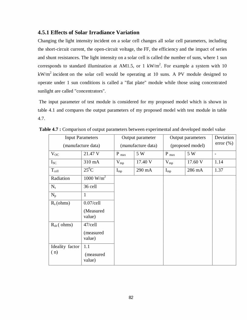
82

4.5.1 Effects of Solar Irradiance Variation

Changing the light intensity incident on a solar cell changes all solar cell parameters, including

the short-circuit current, the open-circuit voltage, the FF, the efficiency and the impact of series

and shunt resistances. The light intensity on a solar cell is called the number of suns, where 1 sun

corresponds to standard illumination at AM1.5, or 1 kW/m2. For example a system with 10

kW/m2 incident on the solar cell would be operating at 10 suns. A PV module designed to

operate under 1 sun conditions is called a "flat plate" module while those using concentrated

sunlight are called "concentrators".

The input parameter of test module is considered for my proposed model which is shown in

table 4.1 and compares the output parameters of my proposed model with test module in table

4.7.

Table 4.7 : Comparison of output parameters between experimental and developed model value

Input Parameters

(manufacture data)

Output parameter

(manufacture data)

Output parameters

(proposed model)

Deviation error (%)

VOC 21.47 V P max 5 W P max 5 W -

ISC 310 mA Vmp 17.40 V Vmp 17.60 V 1.14

Tcell 250C Imp 290 mA Imp 286 mA 1.37

Radiation 1000 W/m2

Ns 36 cell

Np 1

Rs (ohms) 0.07/cell (Measured value)

Rsh ( ohms) 47/cell

(measured value)

Ideality factor ( n)

1.1 (measured value)

83

The I-V and P-V characteristics curve of proposed model is shown in Fig 4.20 and Fig 4.21.

Simulation is done at standard condition (Irradiation 1000 W/m2 and cell temperature 250C).

Fig. 4.20 : Current -Voltage characteristics at Irradiance=1000 W/m2 and Tc =250c

Fig. 4.21: : Power -Voltage characteristics at Irradiance=1000 w/m2

and Tc=250c.

The proposed model includes two subsystems: one that calculates the PV cell photocurrent

which depends on the Irradiance and the temperature according to equation (3.5).

0.00

0.05

0.10

0.15

0.20

0.25

0.30

0.35

0.40

0.00 5.00 10.00 15.00 20.00 25.00

Cur

rent

(A)

Voltage (V)

0.00

1.00

2.00

3.00

4.00

5.00

6.00

0.00 5.00 10.00 15.00 20.00 25.00

Pow

er (

W)

Voltage (V)

84

Based on the equation (3.5), the subsystem of Fig. 4.22 is obtained and the model simulation

results are shown in Figs. 4.23 and 4.24.

Fig. 4.22: Iph Matlab/SIMULINK subsystem for varying cell temperature and solar Irradiance

As it can be seen from Figs.4.23 and 4.24, the PV cell current and Pmax is strongly dependent on

the solar Irradiance.

Fig.4.23: Current-Voltage characteristics for different solar Irradiance.

0.00

0.05

0.10

0.15

0.20

0.25

0.30

0.35

0.00 5.00 10.00 15.00 20.00 25.00

1000 W/m^2800 W/m^2600 W/m^2400 W/m^2

Voltage, (V)

Cur

rent

(A)

85

Fig.4.24: Power-Voltage characteristics for different solar Irradiance.

Simulation Results are compared with experimental results at six different irradiance levels (105

W/m2 to 602 W/m2). It is shown from fig 4.25 to fig 4.36. The summary of this comparing is

shown in table 5.8

Fig 4.25: Simulated and Experimental Current-Voltage characteristics at Irradiance of 105 W/m2

Fig 4.26: Simulated and Experimental Power Voltage characteristics at Irradiance of 105 W/m2

0.00

1.00

2.00

3.00

4.00

5.00

6.00

0.00 5.00 10.00 15.00 20.00 25.00

1000 W/m^2800 W/m^2600 W/m^2400 W/m^2

Voltage, (V)

Pow

er,(W

)

0.00

0.01

0.01

0.02

0.02

0.03

0.03

0.04

0.00 5.00 10.00 15.00 20.00

Experimental data

simulation dataCur

rent

, (A

)

Voltage,(V)

0.00

0.10

0.20

0.30

0.40

0.50

0.00 5.00 10.00 15.00 20.00

Experimental datasimulation data

Voltage,(V)

Pow

er, (

W)

86

Fig 4.27: Simulated and Experimental Current -Voltage characteristics at Irradiance of 202 W/m2

Fig 4.28: Simulated and Experimental Power -Voltage characteristics at Irradiance of 202 W/m2


0.00

0.01

0.02

0.03

0.04

0.05

0.06

0.07

0.00 5.00 10.00 15.00 20.00

Experimental data

simulation data

Voltage,(V)

Cur

rent

, (A

)

0

0.1

0.2

0.3

0.4

0.5

0.6

0.7

0.8

0.00 5.00 10.00 15.00 20.00


Voltage,(V)

Pow

er, (

W)

0.00

0.02

0.04

0.06

0.08

0.10

0.00 5.00 10.00 15.00 20.00 25.00


Voltage,(V)

Curr

ent,

( A)

87


Fig 4.31: Simulated and Experimental Current Voltage characteristics at Irradiance of 400 W/m2


0

0.2

0.4

0.6

0.8

1

1.2

1.4

0.00 5.00 10.00 15.00 20.00 25.00

Experimental data

simulation dataPo

wer

, (W

)

Voltage,(V)

0.00

0.02

0.04

0.06

0.08

0.10

0.12

0.14

0.00 5.00 10.00 15.00 20.00 25.00


Cur

rent

, (A

)

Voltage, (V)

00.20.40.60.8

11.21.41.61.8

0.00 5.00 10.00 15.00 20.00 25.00

experimental data

simulation dataPow

er, (

W)

Voltage, (V)

88




0.00

0.02

0.04

0.06

0.08

0.10

0.12

0.14

0.16

0.18

0.00 5.00 10.00 15.00 20.00 25.00

Experimental data

simulation dataCur

rent

, (A

)

Voltage,(V)

0

0.5

1

1.5

2

2.5

0.00 5.00 10.00 15.00 20.00 25.00

experimental data

simulation data

Voltage,(V)

Pow

er, (

W)

0.000.020.040.060.080.100.120.140.160.180.20

0.00 5.00 10.00 15.00 20.00 25.00


Cur

rent

, (A

)

Voltage,(V)

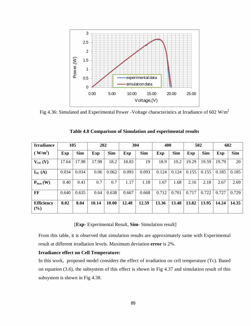
89


Table 4.8 Comparison of Simulation and experimental results

[Exp- Experimental Result, Sim- Simulation result]

From this table, it is observed that simulation results are approximately same with Experimental

result at different irradiation levels. Maximum deviation error is 2%.

Irradiance effect on Cell Temperature: In this work, proposed model considers the effect of irradiation on cell temperature (Tc). Based

on equation (3.6), the subsystem of this effect is shown in Fig 4.37 and simulation result of this

subsystem is shown in Fig 4.38.

0

0.5

1

1.5

2

2.5

3

0.00 5.00 10.00 15.00 20.00 25.00

experimental data

simulation data

Voltage,(V)

Pow

er,(W

)

Irradiance

( W/m2)

105 202 304 400 502 602

Exp Sim Exp Sim Exp Sim Exp Sim Exp Sim Exp Sim

VOC (V) 17.64 17.98 17.98 18.2 18.83 19 18.9 19.2 19.29 19.59 19.79 20

ISC (A) 0.034 0.034 0.06 0.062 0.093 0.093 0.124 0.124 0.155 0.155 0.185 0.185

Pmax (W) 0.40 0.41 0.7 0.7 1.17 1.18 1.67 1.68 2.16 2.18 2.67 2.69

FF 0.640 0.635 0.64 0.638 0.667 0.668 0.712 0.701 0.717 0.722 0.727 0.729

Efficiency (%)

8.02 8.04 10.14 10.00 12.48 12.59 13.36 13.48 13.82 13.95 14.24 14.35

90

Fig 4.37: Tcell Matlab /SIMULINK subsystem for varying solar Irradiance

Fig 4.38: Cell temperature as a function of solar Irradiance

In Fig 4.38, it is observed that cell temperature is dependent on solar Irradiance. Cell temperature

varies from 280c to 580c between 100 W/m2 to 1000 W/m2

4.5.2 Effect of Varying Cell Temperature Temperature plays another major factor in determine the solar cell efficiency. As the temperature

increases the rate of photon generation increases thus reverse saturation current increases rapidly

and this reduces the band gap. Hence this leads to marginal changes in current but major changes

in voltage. The cell voltage reduces by 2.2 mV per degree rise of temperature. Temperature acts

like a negative factor affecting solar cell performance. Therefore solar cells give their full

performance on cold and sunny days rather on hot and sunny weather. Temperature affects the

characteristic equation in two ways: directly, T in the exponential term, and indirectly its effect

on I0 . While increasing T reduces the magnitude of the exponent in the characteristic equation,

0

10

20

30

40

50

60

70

0 200 400 600 800 1000 1200Radiation(W/m2)

Cell

Tem

pera

ture

, Tc

(0 C)

91

the value of I0 increases exponentially with Tc. The net effect is to reduce VOC (the open-circuit

voltage) linearly with increasing temperature. The magnitude of this reduction is inversely

proportional to VOC; that is, cells with higher values of VOC suffer smaller reductions in voltage

with increasing temperature. For most crystalline silicon solar cells the change in VOC with

temperature is about -0.50%/°C, though the rate for the highest-efficiency crystalline silicon cells

is around -0.35%/°C. By way of comparison, the rate for amorphous silicon solar cells is -

0.20%/°C to -0.30%/°C, depending on how the cell is made.

The amount of photo generated current IL increases slightly with increasing temperature because

of an increase in the number of thermally generated carriers in the cell. This effect is slight,

however: about 0.065%/°C for crystalline silicon cells and 0.09% for amorphous silicon cells.

The diode reverse saturation current varies as a cubic function of the temperature. The reverse

saturation current subsystem shown in Fig.4.39 was constructed based on equation 3.7.

Fig.4.39: Matlab/SIMULINK temperature effect subsystem on diode reverses saturation current.

The figure below shows I-V curves that might typically be seen for a crystalline silicon solar cell

at various temperatures. This behaviour is validated and presented in Figs.4.40 and 4.41.

92

Fig.4.40: Current-Voltage characteristics for different cell temperatures.

Fig.4.41: Power-Voltage characteristics for different cell temperatures.

0.000

0.050

0.100

0.150

0.200

0.250

0.300

0.350

0.400

0.000 10.000 20.000 30.000

T=25C

T=50

T=75

Voltage , (V)

Curr

ent ,

(A)

0.000

1.000

2.000

3.000

4.000

5.000

6.000

0.000 10.000 20.000 30.000

T=25C

T=50

T=75

Voltage, (V)

Pow

er,(

W)

93

Fig. VOC as a function of Cell Temperature

Fig.4.43 Isc as a function of Cell Temperature

10.000

12.000

14.000

16.000

18.000

20.000

22.000

24.000

25.000 35.000 45.000 55.000 65.000 75.000

Cell Temperature (T).0C

Volta

ge,V

OC

(V)

0.250

0.270

0.290

0.310

0.330

0.350

25.000 35.000 45.000 55.000 65.000 75.000

Cell Temperature (T).0C

Curr

ent,I

sc (

A)

94

Fig.4.44: Pmax as a function of Cell Temperature .

Fig.4.45: Fill Factor as a function of Cell Temperature.

The overall effect of temperature on cell efficiency can be computed using these factors in

combination with the characteristic equation. However, since the change in voltage is much

stronger than the change in current, the overall effect on efficiency tends to be similar to that on

voltage.

.

0.000

1.000

2.000

3.000

4.000

5.000

6.000

7.000

25.000 35.000 45.000 55.000 65.000 75.000

Cell Tamperature (T). 0C

Pow

er,P

max

(W)

0.500

0.550

0.600

0.650

0.700

0.750

0.800

25.000 35.000 45.000 55.000 65.000 75.000

Cell Temperature(T).0C

Fill

Fact

or, F

F

95

Fig.4.46. Efficiency as a function of Cell Temperature.

In Table 4.9, extracted values of the series and shunt resistances from current-voltage

characteristics of polycrystalline silicon solar cell at different temperatures under constant

illumination (1 kW/m2) are presented. Rs and Rsh SIMULINK subsystem for varying temperature

is obtained in Fig 4.47.

Fig 4.47: Rs and Rsh MATLAB/SIMULINK subsystem for varying Temperature

0.00

2.00

4.00

6.00

8.00

10.00

12.00

14.00

16.00

18.00

25 35 45 55 65 75

Temperature(T).0C

Effic

ienc

y (%

)

96

Table 4.9: Extracted values of Rs and Rsh for the considered crystalline silicon solar cell at

Irradiance of 1kW/m2

T(K) 298 308 318 328 338 348 358

Rs(Ω) 6.92 8.51 10.47 12.88 15.84 19.49 23.97

Rsh(Ω) 1025.38 939.80 866.09 802.15 746.31 697.25 653.88

From the obtained results (Table 4.9), Series resistance increases with an increase in temperature.

the series resistance is a positive temperature coefficient type, so it is possible to make it under

the form [110]:

Where Bs =0.0207K-1 is a coefficient specific to the semiconductor material and Rs0 is the initial

condition resistance. In this simulation, Rs0=0.0145 is considered.

Fig. 4.47 shows the behavior of Rs as a function of temperature. We find that the temperature

increase leads to an increase of the series resistance.

.

Fig. 4.47: Rs as a function of temperature

From Table 4.9, It is observed that Shunt resistance decreases with an increase in temperature.

So, the shunt resistance can be expressed as negative temperature coefficient type [110]:

0

5

10

15

20

25

30

298 308 318 328 338 348 358 368T(k)

Rs (o

hms)

(4.3)

97

Where Bsh= 799.93 K is a coefficient specific to the semiconductor material and Rsh0 is the

initial condition resistance.

Fig. 4.48: Rsh as a function of temperature

Fig. 4.48 shows the behavior of Rsh as a function of temperature. We find that the temperature

increase leads to a decrease in Rsh . Rsh0 =70 ohm is considered in this simulation.

4.5.3 Effect of Varying Rs The series resistance of the PV cell is low, and in some cases, it can be neglected. However, to

render the model suitable for any given PV cell, it is possible to vary this resistance and predict

the influence of its variation on the PV cell outputs. As seen in Fig 4.49 and 5.50, the variation

of Rs affects the slope angle of the I-V curves resulting in a deviation of the maximum power

point.

Fig.4.49 : Current-Voltage characteristics for different Rs.

0

200

400

600

800

1000

1200

298 308 318 328 338 348 358 368T(k)

R sh

(ohm

s)

0.00

0.05

0.10

0.15

0.20

0.25

0.30

0.35

0.00 5.00 10.00 15.00 20.00 25.00

Rs=0

Rs=0.1

Rs=0.3

Rs=0.6

Voltage , (V)

Curr

ent,

(A)

(4.4)

98

Fig.4.50: Power-Voltage characteristics for different Rs

Table 4.10: Simulation Result for the test module of varying Rs Rs(Ω) 0.00 0.10 0.30 0.60

Pmax (W) 5.32 5.01 4.41 3.56

Voc (V) 21.40 21.40 21.40 21.40

Isc (A) 0.31 0.31 0.31 0.31

Pin (W) 31.25 31.25 31.25 31.25

FF 0.80 0.75 0.66 0.54

Eff (%) 17 16 14 11

Consider Tc =250C and Radiation 1000 W/m2

Fig.4.51: Pmax as a function of Rs

0.00

1.00

2.00

3.00

4.00

5.00

6.00

0.00 5.00 10.00 15.00 20.00 25.00

Rs=0

Rs=0.1

Rs=0.3

Rs=0.6

Voltage(V)

Pow

er (W

)

0.00

1.00

2.00

3.00

4.00

5.00

6.00

0.00 0.20 0.40 0.60 0.80Rs,Ohms

P max

, W

99

Fig.4.52: FF as a function of Rs

Fig.5.53: Efficiency as a function of Rs

The simulation was performed for four different values of Rs, namely 0.0Ω, 0.10Ω, 0.30Ω and

0.60 Ω. It was shown that higher values of Rs reduce the power output of the PV cell. The fill

factor also decreases as Rs increases.

4.5.4. Effect of Varying Rsh The shunt resistance of any PV cell should be large enough for higher output power and fill

factor. In fact, for a low shunt resistor, the PV cell current collapses more steeply which means

higher power loss and lower fill factor. These results can be seen in Figs.4.54 and 4.55.

0.000.100.200.300.400.500.600.700.800.90

0.00 0.20 0.40 0.60 0.80

Rs,Ohms

Fill

Fact

or

0.00

2.00

4.00

6.00

8.00

10.00

12.00

14.00

16.00

18.00

0.00 0.20 0.40 0.60 0.80

Effic

ienc

y (%

)

Rs,Ohms

100

Fig.4.54: Current-Voltage characteristics for different Rsh

Fig.4.55: Power-Voltage characteristics for different Rsh

Fig.4.56: Pmax as a function of Rsh

0

0.05

0.1

0.15

0.2

0.25

0.3

0 5 10 15 20 25

Rsh=100 Rsh=10 Rsh=5

Curr

ent

(A)

Voltage (V)

00.5

11.5

22.5

33.5

44.5

5

0 5 10 15 20 25

Rsh=100 Rsh=10 Rsh=5

Voltage (V)

Pow

er (

W)

0.00

0.50

1.00

1.50

2.00

2.50

3.00

3.50

0 50 100 150Rsh (ohms)

P max

(W)

101

Fig.4.57 FF as a function of Rsh

Fig.4.58: Efficiency as a function of Rsh

The simulation is performed for three different values of Rsh, namely 5Ω, 10Ω and100Ω. It is

shown that higher values of Rsh increase the power output of the PV cell. The fill factor also

increases with increasing Rsh .

4.5.5. Effects of Varying I0. If one assumes infinite shunt resistance, the characteristic equation can be solved for VOC:

Thus, an increase in I0 produces a reduction in VOC proportional to the inverse of the logarithm

of the increase. This explains mathematically the reason for the reduction in VOC that

accompanies increases in temperature described above. The effect of reverse saturation current

0.000.100.200.300.400.500.600.700.800.90

0 50 100 150Rsh(ohms)

Fill

Fact

or

0.002.004.006.008.00

10.0012.0014.0016.0018.00

0 50 100 150

Effic

ienc

y (%

)

Rsh(ohms)

(4.4)

102

on the I-V curve of a crystalline silicon solar cell is shown in the figure to the right. Physically,

reverse saturation current is a measure of the "leakage" of carriers across the p-n junction in

reverse bias. This leakage is a result of carrier recombination in the neutral regions on either side

of the junction. The curves of Figs.4.59 and 4.60 were plotted for three different values of I0:

10nA, 1nA and 0.1nA. The influence of an increase in I0 is evidently seen as decreasing the

open-circuit voltage VOC and maximum power Pmax.

Fig.4.59: Current-Voltage characteristics for different I0

Fig.4.60: Power-Voltage characteristics for different I0

0

0.05

0.1

0.15

0.2

0.25

0.3

0.35

0.4

0.45

0.5

0 5 10 15 20 25

Io=0.1nA Io=1nA Io=10nA

Voltage (V)

Curr

ent (

A)

0

1

2

3

4

5

6

0 5 10 15 20 25

Io=0.1nA Io=1nA Io=10nA

Voltage (V)

Pow

er (

W)

103

4.5.6. Effects of Varying Ideality Factor The ideality factor (also called the emissivity factor) is a fitting parameter that describes how

closely the diode's behavior matches that predicted by theory, which assumes the p-n junction of

the diode is an infinite plane and no recombination occurs within the space-charge region. A

perfect match to theory is indicated when n = 1. When recombination in the space-charge region

dominate other recombination, however, n = 2. Most solar cells, which are quite large compared

to conventional diodes, well approximate an infinite plane and will usually exhibit near-ideal

behavior under Standard Test Condition (n ≈ 1). Under certain operating conditions, however,

device operation may be dominated by recombination in the space-charge region.

The ideality factor, also known as the quality factor varies from 1 to 2 depending on the

fabrication process and semiconductor material, see in (Fig. 4.61) and (fig. 4.62) show that with

increasing the diode quality factor reduces the maximum power that the panel could provide in

addition, deteriorating fill factor, because although ISC and VOC does not change, if it does the

curvature of the knee where the maximum power occurs.

Fig 4.61: Current-Voltage characteristic as a function of diode ideality factor

Fig 4.62: Power-Voltage characteristic as a function of diode ideality factor

0

0.1

0.2

0.3

0 5 10 15 20 25

n=1 n=1.33 n=1.66 n=2

Voltage (V)

Curr

ent (

A)

0

1

2

3

4

5

6

0 5 10 15 20 25

n=1 n=1.33 n=1.66 n=2

Pow

er (W

)

Voltage (V)

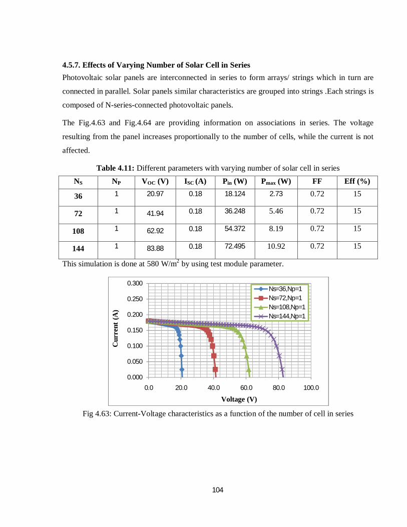
104

4.5.7. Effects of Varying Number of Solar Cell in Series Photovoltaic solar panels are interconnected in series to form arrays/ strings which in turn are

connected in parallel. Solar panels similar characteristics are grouped into strings .Each strings is

composed of N-series-connected photovoltaic panels.

The Fig.4.63 and Fig.4.64 are providing information on associations in series. The voltage

resulting from the panel increases proportionally to the number of cells, while the current is not

affected.

Table 4.11: Different parameters with varying number of solar cell in series NS NP VOC (V) ISC (A) Pin (W) Pmax (W) FF Eff (%)

36 1 20.97 0.18 18.124 2.73 0.72 15

72 1 41.94 0.18 36.248 5.46 0.72 15

108 1 62.92 0.18 54.372 8.19 0.72 15

144 1 83.88 0.18 72.495 10.92 0.72 15

This simulation is done at 580 W/m2 by using test module parameter.

Fig 4.63: Current-Voltage characteristics as a function of the number of cell in series

0.000

0.050

0.100

0.150

0.200

0.250

0.300

0.0 20.0 40.0 60.0 80.0 100.0

Ns=36,Np=1Ns=72,Np=1Ns=108,Np=1Ns=144,Np=1

Voltage (V)

Cur

rent

(A)

105

Fig 4.64: Power-Voltage characteristics as a function of the number of cell in series

Fig 4.65: Rs as a function of the number of cell in series

Fig 4.66: Rsh as a function of the number of cell in series

0.00

2.00

4.00

6.00

8.00

10.00

12.00

0.0 20.0 40.0 60.0 80.0 100.0

Ns=36,Np=1Ns=72,Np=1Ns=108,Np=1Ns=144,Np=1

Voltage (V)

Pow

er (W

)

0.00

10.00

20.00

30.00

40.00

50.00

60.00

0 50 100 150 200

No. of cell in series (Ns)

Rs (

ohm

s)

0.00500.00

1000.001500.002000.002500.003000.003500.004000.004500.005000.00

0 50 100 150 200

No. of cell in series (Ns)

Rsh

(ohm

s)

106

Fig 4.67: Simulated and Experimental current voltage characteristics of two modules in series at

Irradiance of 580 W/m2

Fig 4.68: Simulated and Experimental power voltage characteristics of two modules in series at


Table 4.12 Comparison of Simulation and Experimental value for two modules in series

Experimental Value Simulation Data Deviation error (%) VOC (V) 40 V 41.5 V 1.2

ISC (A) 0.18A 0.18 --

Pmax (W) 5.41 W 5.46 W 0.9

It is found that both results are approximately same.

0.000

0.050

0.100

0.150

0.200

0.250

0.300

0.0 10.0 20.0 30.0 40.0 50.0

Ns=72,Np=1(Experimental data)Ns=72,Np=1(Simulation data)

Voltage(V)

Cur

rent

(A)

0.00

2.00

4.00

6.00

8.00

10.00

12.00

0.0 10.0 20.0 30.0 40.0 50.0

Ns=72,Np=1( Experimental data)

Ns=72,Np=1(Simulation Data)

Pow

er(W

)

Voltage(V)

107

4.5.8. Effects of varying number of solar cell in parallel The Fig.4.69 and Fig.4.70 are providing information on associations in parallel. The resulting

intensity of the panel increase proportionally to the number of cells, while the voltage is not

affected. It is observed that the power supplied by the panel is equal in both cases, since a

proportional increase of the current.

Table 4.13: Different parameters with varying number of solar cell in parallel NS NP VOC (V) ISC (A) Pin (W) Pmax (W) FF Eff (%)

36 1 20.97 0.18 18.124 2.73 0.72 15

36 2 20.97 0.359 36.248 5.46 0.72 15

36 3 20.97 0.539 54.372 8.19 0.72 15

36 4 20.97 0.719 72.495 10.92 0.72 15

Fig 4.69: I-V characteristics as a function of the number of cells in parallel

Fig 4.70: P-V characteristics as a function of the number of cells in parallel

0.0000.1000.2000.3000.4000.5000.6000.7000.8000.9001.000

0.0 5.0 10.0 15.0 20.0 25.0

Ns=36,Np=1

Ns=36,Np=2

Ns=36,Np=3

Ns=36,Np=4

Voltage(V)

Cur

rent

(A)

0.000

2.000

4.000

6.000

8.000

10.000

12.000

0.0 5.0 10.0 15.0 20.0 25.0

Ns=36,Np=1

Ns=36,Np=2

Ns=36,Np=3

Ns=36,Np=4

Voltage(V)

Pow

er(W

)

108

Fig 4.71: Rs characteristics as a function of the number of cells in parallel

Fig 4.72: Rsh characteristics as a function of the number of cells in parallel

Fig 4.73: Simulated and Experimental current voltage characteristics of two modules in parallel

at Irradiance of 580 W/m2

0.00

2.00

4.00

6.00

8.00

10.00

12.00

14.00

0 1 2 3 4 5No. of cell in parallel (Np)

Rs(

ohm

s)

0.00

200.00

400.00

600.00

800.00

1000.00

1200.00

0 2 4 6No. of cell in parallel (Np)

Rsh

(ohm

s)

0.000

0.100

0.200

0.300

0.400

0.500

0.600

0.0 5.0 10.0 15.0 20.0 25.0


Voltage (V)

Cur

rent

(A)

109

Fig 4.74: Simulated and Experimental power voltage characteristics of two modules in parallel at


Table 4.14 Comparison of Simulation and Experimental value for two modules in Parallel

Experimental Value Simulation Data Deviation error (%) Voc (V) 19.1 19.6 2.5 Isc (A) 0.36 0.36 --

Pmax (W) 5.47 5.46 0.2 It is found that both results are approximately same. 4.5.9 Simulation for cell, module and array In this model, 36 PV cell are interconnected in series to form one module. As a result, the

module voltage is obtained by multiplying the cell voltage by the cells number while the total

module current is the same as the cell’s one. The results are shown in Figs.4.79 and 4.80.

Fig.4.75. SIMULINK model for the PV module.

In order to get benefit from these developed models, an array of PV modules has been

constructed. In fact, these PV modules were interconnected in series and all of them are

connected to the external control block as shown in Fig.4.76.

0.000

2.000

4.000

6.000

8.000

10.000

12.000

0.0 5.0 10.0 15.0 20.0 25.0


Voltage (V)

Pow

er (w

)

110

Fig.4.76: SIMULINK model for the PV array

The PV array model is simulated similarly to the model of the PV module and the obtained

results are shown in Figs.4.81 and 4.82, respectively. All simulations are done at standard test

condition (G=1000 W/m2 and T= 250C). Consider three modules are connected in series for array

simulation.

Fig 4.77: Current-Voltage characteristics of a cell for test module

00.05

0.10.15

0.20.25

0.30.35

0.4

0 0.2 0.4 0.6 0.8Voltage (V)

Cur

rent

(A)

111

Fig 4.78: Power-Voltage characteristics of a cell for test module

Fig 4.79: Current-Voltage characteristics for the test module

Fig 4.80: Power-Voltage characteristics for the test module

0

0.05

0.1

0.15

0.2

0.25

0.3

0 0.2 0.4 0.6 0.8

Pow

er (

W)

Voltage (V)

0.00

0.05

0.10

0.15

0.20

0.25

0.30

0.35

0.40

0.00 5.00 10.00 15.00 20.00 25.00Voltage (V)

Cur

rent

(A)

0.00

1.00

2.00

3.00

4.00

5.00

6.00

0.00 5.00 10.00 15.00 20.00 25.00

Pow

er (

W)

Voltage (V)

112

Fig 4.81: Current-Voltage characteristics of array for test module

Fig 4.82: Power-Voltage characteristics of array for test module

Three modules are connected in series for array simulation.

4.6. Experimental Results and Validation In order to validate the Matlab/SIMULINK model, The PV test module of Fig 4.83 was

investigated. The key specifications are listed in Table 4.14.

0

0.05

0.1

0.15

0.2

0.25

0.3

0.35

0.4

0 20 40 60 80Voltage (V)

Cur

rent

(A)

0

2

4

6

8

10

12

14

16

18

0 20 40 60 80

Pow

er (W

)

Voltage (V)

113

Fig 4.83: Test Module (JKM250M-60)

Table 4.15 Key specification of Test Module (JKM250M-60) Model:JKM250M-60 Maximum power(Pmax) 250w Open circuitVoltage(Voc) 31.7V Short circuit current(Isc) 8.70 A Voltage at Pmax 30.6 V Current at Pmax 8.17A Module dimensions 1650×992×45mm Module weight 19kg Cell type Mono crystalline No.of cells 60 cells in series Data measured in standard condition(STC):Irradiation 1000 W/m2,AM1.5,cell temperature 250C,Tested according to:IEC 61215 and IEC 61730

The Matlab/SIMULINK model is evaluated for the JKM250M-60 solar panel. The results are

shown in Fig.4.84 and 4.85. On the other hand, the experimental results for a solar radiation of

580 W/m2 are shown in Fig. 4.86 and 4.87.

114

Fig4.84: Simulation result of Current-Voltage characteristics at 580 W/m2

Fig4.85: Simulation result of Power-Voltage characteristics at 580 W/m2

Fig4.86: Experimental results of Current-Voltage characteristics at 580 W/m2

0

1

2

3

4

5

6

0 10 20 30

Voltage (V)

Curr

ent (

A)

Voc=34

0

20

40

60

80

100

120

140

0 10 20 30Voltage (V)

Pow

er (W

)

Pmax=132W

Voc=34

0

1

2

3

4

5

6

0 10 20 30

Voltage (V)

Curr

ent (

A)

Voc=33.65

115

Fig4.87: Experimental Results of P-V curve at 580 W/m2

Fig 4.88: Simulated and Experimental current voltage characteristics at Irradiance of 580 W/m2

0

20

40

60

80

100

120

140

0 10 20 30

Voltage(v)

Pow

er(W

)

Pmax=130 W

Voc=33.65

0

1

2

3

4

5

6

0 10 20 30 40

Experimental data

simulation dataCur

rent

(A)

Voltage(v)

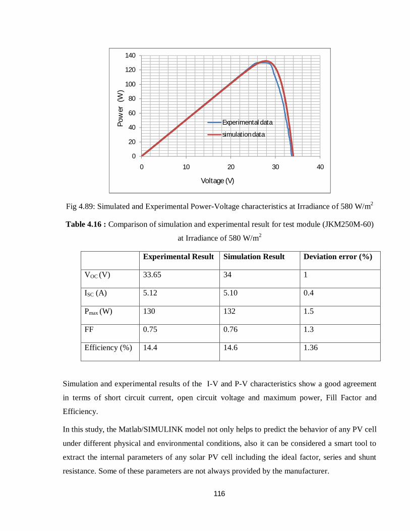
116

Fig 4.89: Simulated and Experimental Power-Voltage characteristics at Irradiance of 580 W/m2

Table 4.16 : Comparison of simulation and experimental result for test module (JKM250M-60)

at Irradiance of 580 W/m2

Experimental Result Simulation Result Deviation error (%)

VOC (V) 33.65 34 1

ISC (A) 5.12 5.10 0.4

Pmax (W) 130 132 1.5

FF 0.75 0.76 1.3

Efficiency (%) 14.4 14.6 1.36

Simulation and experimental results of the I-V and P-V characteristics show a good agreement

in terms of short circuit current, open circuit voltage and maximum power, Fill Factor and

Efficiency.

In this study, the Matlab/SIMULINK model not only helps to predict the behavior of any PV cell

under different physical and environmental conditions, also it can be considered a smart tool to

extract the internal parameters of any solar PV cell including the ideal factor, series and shunt

resistance. Some of these parameters are not always provided by the manufacturer.

0

20

40

60

80

100

120

140

0 10 20 30 40

Experimental data

simulation data

Pow

er (

W)

Voltage (V)

117

CHAPTER 5

Conclusions and Suggestions for Future Works

5.1 Conclusions This chapter summarizes the central features of this research and its outcomes. This is followed

by the plan for future research work. A generalized PV model which is representative of the all

PV cell, module, and the array has been developed with Matlab/Simulink and been verified with

a PV cell and a commercial module. The proposed model takes solar irradiance and cell

temperature as input parameters and outputs the I-V and P-V characteristics under various

conditions. This model has also been designed in the form of Simulink block libraries. Such a

generalized PV model is easy to be used for the implementation on Matlab/Simulink modeling

and simulation platform. 5 watt crystalline solar modules are used in this work.

In this work, analyzing the effect of irradiance on I-V and P-V characteristics and different

parameters of solar module and compare all experimental data with the simulation result of

developed model. The observation is done from 105 W/m2 to 602 W/m2. Simulation results are

approximately same with experimental results. When analyzing the effect of irradiance, it is

observed that short circuit current (Isc) has proportionally increased with increasing Irradiance

and Voc is very small with increasing irradiance. Maximum power (Pmax) also proportionally

increases with increasing solar irradiance. Fill Factor and efficiency is gradually rising with

increasing irradiance.

It is extracted the value of series and shunt resistance from the I-V characteristic of the solar

module at different irradiation levels. Series resistance is gradually decreasing with increasing

solar irradiance. This resistance varies from 128.15 ohms to 14.35 ohms between 105 W/m2 to

602 W/m2. But the change of shunt resistance is not large.

In this work, It has developed an empirical equation for the Irradiance effect on the series

resistance of solar cell by using experimental data. Developed equation is valid for another

experimental data. Maximum deviation error 7%.

118

It is also extracted the value of the ideality factor from the I-V characteristics of solar module at

different irradiation levels. It is observed that ideality factor decreases with increasing solar

irradiance. It varies from 2.5 to 1.2 with varying 105 W/m2 to 602 W/m2.

In this study, comparing the efficiency between monocrystalline and polycrystalline solar

module. Using manufacturer’s input parameters; it verifies the output parameters of simulation

result of my proposed model with end product data of the manufacturer. Deviation error is found

1.37% of this verification.

It has also examined the effect of varying the number of solar cells in series and parallel.

Experimental and simulation data are approximately same for this work. In series condition, the

voltage increases with increasing number of cells, but current is not affected. In parallel

condition, current increases with increasing number of cells but voltage is not affected. But the

change of maximum power is equal in both cases. Parasitic resistance increases with increasing

the solar cell in series and decreases with increasing solar cell in parallel.

The effect of parasitic resistance is also analyzed in this work. The ISC and VOC remain constant

but the maximum power point is varying. The series resistance influences the slope of the I-V

Characteristics at the constant voltage region. At the same time parallel resistance Rsh influences

the slope of the curve at the constant current region. Pmax, FF and Efficiency gradually decreases

with increasing series resistance and inverse situation is occurred for shunt resistance.

Temperature effect on different parameters of the solar module is reported in this work only

simulation basis. From I-V and P-V characteristics, it is observed that Voc reduces linearly with

increasing temperature, but the change of ISC is very small. FF, Maximum power and efficiency

gradually decreases with increasing temperature. It is also observed that Rs increases and Rsh

decreases with increasing temperature.

From this work, one can extract the different physical parameters of the solar cell from I-V and

P-V characteristic in particular Irradiance level and using all of parameters, it is possible to

simulate I-V and P-V characteristics at another Irradiance level without experiment.

119

5.2 Further Works

The simulations have been presented here on a silicon solar cell; merely it is generalized to all kinds of solar cell. Thus, high efficiency solar cells can be effectively simulated using the above model.

Due to time constraint for this project, further research could be done to identify a better model

for parallel PV cells for partial shading. To further increase the accuracy of the predictions, it is

suggested that the manufacturers provide two sets of data at two different reference conditions.

Further research could be exercised on the performance impact of different types of solar

material. Finally, it is also suggested that the manufacturers provide either a complete current-

voltage curve, at the reference condition so that the parameters for modeling the panel

performance can be determined.

In this study, it is experimentally demonstrated that an ideality factor varies with varying solar

irradiance. In future, this effect may be considered for modeling.

A Photovoltaic system doesn’t just consist of PV modules, but also involves a good deal of

power electronics as an interface between PV modules and load for effective and efficient

utilization of naturally available Sun power. Such a PV model is easy to be used for the

implementation on Matlab/Simulink modeling and simulation platform. In future, both PV

modules and the associated power electronics under different operating conditions and load may

be simulated by using Simulink.

The proposed model has a generalized structure so that it can be used as a PV power generator

along with wind, fuel cells and small hydro system by establishing proper interfacing and

controllers. The model may be simulated with connecting a three phase inverter and interfaced to

AC loads as well as the AC utility grid system. Therefore the model proposed here can be

considered as a part of distributed power generation systems.

The applications of photovoltaic will increase both for small-decentralized power supplies and

for large power stations. This makes a significant energy contribution. The rate of this progress

will depend on the amount of expert knowledge, contributes by those involved in the planning,

construction and operation of PV system.

120

References

[1] T. Esram, P. L. Chapman, "Comparison of Photovoltaic Array Maximum Power Point

Tracking Techniques," IEEE Transactions on Energy Conversion, Vol. 22, No. 2, June

2007, pp. 439 - 449.

[2] Vorster F.J., van Dyk E.E., Leitch A.W.R., "Investigation on the I-V characteristics of a

high concentration, photovoltaic array", Conference Record of the Twenty-Ninth IEEE

Photovoltaic Specialists Conference, pp.1604-1607, 2002.

[3] Tariq salmi,Mounir Bouzguenda,Adel Gastil, “MATLAB/Simulink based modeling of

solar photovoltaic cell”, International Journal of renewable energy research, vol. 2, No. 2,

2012

[4] N. D. Benavides and P. L. Chapman, “Modeling the effect of voltage ripple on the power

output of photovoltaic modules,” IEEE Trans. Ind.Electron., Vol. 55, No. 7, pp. 2638–

2643, Jul. 2008.

[5] Savita Nema, R.K. Nema, Gayatri Agnihotri, “MATLAB/Simulink based study of

photovoltaic cells and their experimental verification”, International journal of Energy

and Environment, vol.1, No.3, pp.487-500, 2010.

[6] Huan-Liang Tsai, Ci-Siang Tu, Yi-Jie Su, “Development of Photovoltaic Model Using

MATLAB/SIMULINK”, Proceedings of the World Congress on Engineering and

Computer Science WCECS, San Francisco, USA, 2008.

[7] Jeyraj Selvaraj, Nasrudin A. Rahim, “Multilevel Inverter For Grid-Connected PV System

Employing Digital PI Controller”, IEEE Transactions On Industrial Electronics, vol. 56,

No. 1, pp. 149-158 , 2009.

[8] S. Rustemli, F. Dincer, “Modeling of Photovoltaic Panel and Examining Effects of

Temperature in Matlab/Simulink”, Electronics and Electrical Engineering, ISSN 1392-

1215, no. 3(109), pp. 35-40, 2011.

121

[9] Kinal Kachhiya, Makarand Lokhande, Mukesh Patel, “ Model of Solar PV Module and

MPPT Algorithm”, Proceedings of the National Conference on Recent Trends in

Engineering and Technology, 2011

[10] Pradhan Arjyadhara1, Ali S.M2, Jena Chitralekha3, “ Analysis of Solar PV cell

Performance with Changing Irradiance and temperature”, International Journal Of

Engineering And Computer Science ISSN:2319, Volume 2, Issue 1, Jan 2013 .

[11] C. C. Hua and C. M. Shen, “Study of maximum power tracking techniques and control of

dc-dc converters for photovoltaic power system,” Proceedings of 29th annual IEEE

Power Electronics Specialists Conference, vol. 1, 1998, pp. 86-93.

[12] Y. Jiang, J.A.A. Qahouq, M. Orabi, Matlab/Pspice hybrid simulation modeling of solar

PV cell/module, in: 26th Annual IEEE Applied Power Electronics Conference and

Exposition (APEC), Fort Worth, TX, 2011, pp.1244-1250.

[13] S. Moballegh, J. Jiang, Partial shading modeling of photovoltaic system with

experimental validations, in: 2011 IEEE Power and Energy Society General Meeting, San

Diego, CA, 2011, pp. 1-9.

[14] K. Ishaque, Z. Salam, H. Taheri, Accurate MATLAB simulink PV system simulator

based on a two-diode model, Journal of Power Electronics 11 (2011) 179-187.

[15] J.T. Bialasiewicz, Renewable energy systems with photovoltaic power generators:

Operation and modeling, IEEE Transactions on Industrial Electronics 55 (2008) 2752-

2758.

[16] International Energy Agency, "2012 Energy Balance for World", 2012 .

[17] http://en.wikipedia.org/wiki/Electricity_generation.

[18] M. Asif, and T. Muneer (2007). Energy supply, its demand and security issues for

developed and emerging economies. Renewable and Sustainable Energy Reviews, 11(7),

pp. 1388-1413.

[19] Barton, J.H. (2007). Intellectual Property and Access to Clean Energy Technologies in

Developing Countries: An Analysis of Solar Photovoltaic, Biofuel, and Wind

122

Technologies. Issue Paper No. 2, International Center for Trade and Sustainable

Development, Geneva, Switzerland.

[20] Bazilian, M., and F. Roques (2008). Analytical Methods for Energy Diversity And

Security: Mean-Variance Optimization for Electric Utilities Planning: A Tribute to the

Work of Dr. Shimon Awerbuch. 1st ed. Elsevier, Boston, MA, USA.

[21] REN21 – 2013 Renewables Global Status Report, http:// www.ren21.net/Portals/ 0/ documents / Resources/GSR/2013/GSR2013_lowres.pdf

[22] Bruce, A., M.E. Watt, and R. Passey (2009), A survey ofNew South Wales residential PV

rebate recipients. In: 47th Annual Conference of the Australia and New Zealand Solar

Energy Society, Townsville, Australia, 29 September – 2 October 2009.

[23] Bruckner, T., O. Edenhofer, H. Held, M. Haller, M. Lüken, N. Bauer, and N.

Nakicenovic (2010). Robust options for decarbonisation. In: Global Sustainability,

Cambridge University Press, pp. 189-204.

[24] Butler, L., and K. Neuhoff (2008). Comparison of feed-in tariff, quota, and auction

mechanisms to support wind power development. Renewable Energy, 33(8), pp. 1854-

1867.

[25] Chaurey, A., and T. Kandpal (2010). Assessment and evaluation of PV based

decentralized rural electrification: An overview. Renewable and Sustainable Energy

Reviews, 14(8), pp. 2266-2278.

[26] Clarke, L., J. Edmonds, V. Krey, R. Richels, S. Rose, and M. Tavoni (2009).

International climate policy architectures: Overview of the EMF 22 International

Scenarios. Energy Economics, 31(Supplement 2), pp. 64-81.

[27] Cossent, R., T. Gomez, and P. Frias (2009). Towards a future with large penetration of

distributed generation: Regulatory ecommendations under a European perspective.

Energy Policy, 37, pp. 1145-1155

[28] Demirbas, A. (2009). Global renewable energy projections. Energy Sources, 4, pp. 212-

224

[29] B.G. Streetman, Solid State Electronic Devices. Prentice Hall, 2000.

123

.

[30] R. Corkish, Luke, K. L., Altermatt, P. P., and Heiser, G., “Simulating Electron-Beam-

Induced Current Profiles Across p-n Junctions”,16h European Solar Energy Conference.

pp. 1590-1593, 2000

[31] Groothuis, P.A., J.D. Groothuis, and J. C. Whitehead (2008). Green vs. green: Measuring

the compensation required to site electrical generation windmills in a viewshed. Energy

Policy, 36(4), pp. 1545-1550

[32] A. Luque and Hegedus, S., “Handbook of Photovoltaic Science and Engineering”, p.

1117, 2003.

[33] J. Nelson, “The Physics of Solar Cells”, p. 355, 2003.

[34] Kooles, K. (2009). Adapting historic district guidelines for solar and other green

technologies. Forum Journal, 24, pp. 24-29.

[35] P. P. Altermatt, Schenk, A., Geelhaar, F., and Heiser, G., “Reassessment of the intrinsic

carrier density in crystalline silicon in view of band-gap narrowing”, Journal of Applied

Physics, vol. 93, no. 3, p. 1598, 2003.

[36] P. Campbell and Green, M. A., “High performance light trapping textures for

monocrystalline silicon solar cells”, Solar Energy Materials and Solar Cells, vol. 65, no.

1-4, pp. 369 - 375, 2001.

[37] Bolton, James (1977). Solar Power and Fuels. Academic Press, Inc. ISBN 0-12-112350-

2.

[38] S. R. Wenham, Green, M. A., Watt, M. E., and Corkish, R., “Applied Photovoltaics”, p.

317, 2007.

[39] Gan, J.; Smith, C.T. 2006. Availability of logging residues and potential for electricity

production and carbon displacement in the USA. Biomass and Bioenergy. 30: 1011–

1020.

[40] K. Bothe, Sinton, R., and Schmidt, J., “Fundamental boron-oxygen-related carrier

lifetime limit in mono- and multicrystalline silicon”, Progress in Photovoltaics: Research

and Applications, vol. 13, pp. 287 - 296, 2005.

124

[41] R. Swanson, “Approaching the 29% limit efficiency of silicon solar cells”, Thirty-First

IEEE Photovoltaic Specialists Conference. 01/2005, Lake buena Vista, FL, USA, pp.

889-94, 2005.

[42] M. A. Green and Keevers, M. J., “Optical properties of intrinsic silicon at 300

K”, Progress in Photovoltaics: Research and Applications, vol. 3, pp. 189 - 192, 1995.

[43] P. A. Basore, “Defining terms for crystalline silicon solar cells”, Progress in

Photovoltaics: Research and Applications, vol. 2, pp. 177-179, 1994.

[44] M. M. Hasan, M.F. Khan, “A comparative study on installation of solar PV system for

grid and non grid rural areas of Bangladesh”, Developments in Renewable Energy

Technology (ICDRET), 2012

[45] Mir Nahidul Ambia, Md. Kafiul Islam, Md. Asaduzzaman Shoeb, Md. Nasimul Islam

Maruf, A.S.M. Mohsin, “An Analysis & Design on Micro Generation of A Domestic

Solar-Wind Hybrid Energy System for Rural & Remote Areas-Perspective Bangladesh.”

2010

[46] Andrew Blakers and Klaus Weber, “The Energy Intensity of Photovoltaic Systems”,

Centre for Sustainable Energy Systems, Australian National University, 2009

[47] Alsema, E.A.; Wild - Scholten, M.J. de; Fthenakis, V.M. Environmental impacts of PV

electricity generation - a critical comparison of energy supply options ECN, September

2006; 7p. Presented at the 21st European Photovoltaic Solar Energy Conference and

Exhibition, Dresden, Germany, 4–8 September 2006

[48] Šúri M., Huld T.A., Dunlop E.D. Ossenbrink H.A., 2007. Potential of solar electricity

generation in the European Union member states and candidate countries. Solar Energy,

81, 1295–1305

[49] Choudhury, Debasish (20 August 2009). "Lieberose solar farm becomes Germany's

biggest, World's second-biggest". Global Solar Technology.

[50] Roca, Mark (December 29, 2012). "Europe’s Biggest Solar Park Completed With

Russian Bank Debt".

[51] Martin, Christopher L.; Goswami, D. Yogi (2012). Solar Energy Pocket Reference. International Solar Energy Society. ISBN 0-9771282-0-2

125

[52] http://www.nrel.gov/pv/high_performance_pv.html

[53] Perlin, John (1999). From Space to Earth (The Story of Solar Electricity). Harvard University Press. ISBN 0-674-01013-2

[54] Tiwari, G. N.; Singh, H. N.; Tripathi, R. (2003). "Present status of solar distillation". Solar Energy 75 (5):367–373. Bibcode: 2003SoEn...75..367T. doi:10.1016/j. solener.2003.07.005

[55] Mazria, Edward (1997). The Passive Solar Energy Book. Rondale Press. ISBN 0-87857-238-4

[56] S. C. Baker-Finch, McIntosh, K. R., and Terry, M. L., “Isotextured Silicon Solar Cell Analysis and Modeling 1: Optics”, IEEE Journal of Photovoltaics, vol. 2, no. 4, pp. 457 - 464, 2012.

[57] Andreea Maria Neaca and Mitica Iustinian Neaca, 2009. Modeling photovoltaic systems for AC appliances.Journal of Electrical and Electronics Engineering, 2(2): 58-63.

[58] Chenni, R., M. Makhlouf, T. Kerbache and A. Bouzid, 2005. A Detailed Modelling Method for Photovoltaic Cells. Energy (Elsevier), 32(9): 1724-1730.

[59] Francisco M. Gonzalez-Longatt, 2005. Model of Photovoltaic in Matlab TM. 2do Congreso Iberoamericano de Estudiantes de Ingeniería Eléctrica. Electrónicay Computación (II CIBELEC 2005), pp: 1-5.

[60] Huan-Liang Tsai., Ci-Siang Tu and Yi-Jie Su, 2008. Development of Generalized Photovoltaic ModelUsing MATLAB/SIMULINK. Proceedings of the World Congress on Engineering and Computer Science (WCECS).

[61] E.M.G. Rodrigues, R. Melicio and V.M.F Mendes, “Simulation of a Solar Cell Considering Single Diode Equivalent Circuit Model”, International Journal of Electrical and Computer Engineering (IJECE),2(1): 34-42

[62] M. G. Villalva, J. R. Gazoli, and E. R. Filho, “Comprehensive approach to modeling and

simulation of photovoltaic arrays”, IEEE Transactions on Power Electronics, Vol. 24, No.

5, pp. 1198-1208, May 2009..

[63] A. S. Sedra and K. C. Smith, Microelectronic Circuits. London, U.K.: Oxford Univ.

Press, 2006.

[64] G.R. Walker, “Evaluating MPPT topologies using a Matlab PV model”, Journal of

Electrical & Electronics Engineering, Vol. 21, No. 1, pp. 49-56, 2001.

126

[65] “Photovoltaic systems technology,” Universitat Kassel, Kassel, Germany, 2003.

[66] J. Yuncong, J.A.A. Qahouq, and I. Batarseh, “Improved solar PV cell Matlab simulation model and comparison”, in: Proc. 2010 IEEE International Symposium on Circuits and Systems — ISCAS’10, Tuscalosa, Alabama, USA, 2010.

.[67] W. Xiao, W.G. Dunford, A. Capel, A Novel Modeling Method for Photovoltaic Cells, 35 Annual IEEE Power Electronics Specialists Conference, Aachen, Germany, June 20-25, 2004, 1950-1956

[68] M.G. Villalva, J.R. Gazoli, E.R. Filho, Comprehensive Approach to Modeling and Simulation of Photovoltaic Arrays, IEEE Transactions on Power Electronics 24 (2009) 1198-1208

[69] W. Kim, W. Choi, A novel parameter extraction method for the one-diode solar cell model,Solar Energy 84 (2010) 1008-1019

[70] A. Bellini, S. Bifaretti, V. Iacovone, C. Cornaro, Simplified model of a photovoltaic module, Applied Electronics International Conference (2009) 47-52

[71] J.A. Duffie, W.A. Beckman, Solar Engineering of Thermal Processes, 3th edition, Wiley, Hoboken, New Jersay ,USA (2006)

[72] E. Saloux, A. Teyssedou and M. Sorin, Explicit model of photovoltaic panels to determine voltages and currents at the maximum power point, Solar Energy ,80 (2006),78-88.

[73] S. SINGER, B. ROZENSHTEIN and S. SAURAZI, “Characterization of PV array output using a small number of measured parameters”. Solar Energy, Vol.32, No5, pp.603-607,1984.

[74] D. S. H. CHAN, J. R. PHILIPS and J. C. H. PHANG, “A comparative study of extraction methods for solar cell model parameters”. Solid State Electronics, Vol. 37, pp.123-132, 1995.

[75] J.A. GOW, C.D. MANNING, “Development of a photovoltaic array model for use in power-electronics simulation studies”. IEEE Proc.Electr. Power Appl., Vol. 146,No.2, pp.193-200, 1999 .

[76] Surya K. J., Sai B. Ch., Mathematical Modeling and Simulation of Photovoltaic Cell using Matlab-Simulink Environment, Intr. Jour. of Electrical and Computer Eng. (IJECE), 2007, 2(1), p. 26-34.

[77] M.Abdulkader, A.S.Samosir and A.H.M.Yatim”Modeling and Simulation based approach of photovoltaic system in simulink model” ARPN Journal of engineering and Applied Sciences,vol.7,N0.5, May 2012;.

127

[78] Adamo, F., F. Attivissimo, A. Di Nisio, A.M.L. Lanzolla and M. Spadavecchia, 2009. Parameters estimation for a model of photovoltaic panels. Proc. 19th IMEKO World Congress, Fundamental and Applied Metrology, pp: 964-967.

. [79] Hamdaoui, M., A. Rabhi, A. El Hajjaji, M. Rahmoun and M. Azizi, 2009. Monitoring and control of the performances for photovoltaic systems. Proc. IREC’09, International Renewable Energy Congress (IREC), pp:69-71.

[80] Kashif Ishaque., Zainal Salam and Hamed Taheri, 2011. Accurate MATLAB Simulink PV SystemSimulator Based on a Two-Diode Model. Journal of Power Electronics, 11(2): 179-187.

[81] Lasnier, F and T. G. Ang, 1990. Photovoltaic engineering handbook. New York: Taylor & Francis.

[82] Marcelo Gradella Villalva., Jonas Rafael Gazoli and Ernesto Ruppert Filho, 2009.

Modeling and circuit based simulation of photovoltaic arrays. Power Electronics

Conference (COBEP‘09), pp: 1244-1254.

[83] Mrabti, T., M. El Ouariachi, F. Yaden, Ka. Kassmi and K. Kassmi, 2010.

Characterization and Modeling of the Electrical Performance of the Photovoltaic Panels

and Systems. Journal of Electrical Engineering: Theory and Application, 1(2): 100-110.

[84] Geoff Walker, “Evaluating MPPT converter topologies using a MATLAB PV model”, J.

Elect. Electron. Eng. Australia, vol. 21, pp. 49–56, 2001.

[85] Rahman, H.A., K.M. Nor, M.Y. Hassan, S. Thanakodi, M.S. Majid and F. Hussin, 2010.

Modeling and Simulation of Grid Connected Photovoltaic System for Malaysian Climate

Using Matlab/Simulink. 2010 IEEE International Conference on Power and Energy

(PECon), pp: 935-940.

[86] Ramos Hernanz, J.A., J.J. Campayo Martin, I. Zamora Belver, J. Larranaga Lesaka, E.

Zulueta Guerrero, E.Puelles Perez, 2010. Modelling of Photovoltaic Module.

International Conference on Renewable Energies andPower Quality (ICREPQ’10).

[ 87] Dominique Bonkoungou, Zacharie Koalaga and Donatien Njomo, “Modelling and

Simulation of Photovoltaic Module Considering Single Diode equivalent Circuit Model

128

in Matlab (International Journal of Emerging Technology and Advanceed Engineeringl

Engineering),2013, 3(3): pp.493-502.

[88] Rodrigues, E.M.G., R. Melicio, V.M.F. Mendes and J.P.S. Catalao, 2011. Simulation of a

Solar Cell considering Single-Diode Equivalent Circuit Model. In: ICREPQ’11

International conference on renewable energies and power quality, pp: 1-5.

[89] M.G. Villalva, J.R. Gazoli, E. Ruppert “Modeling and Circuit Based Simulation of

Photovoltaic Arrays”, Brazilian Journal of Power Electronics, Vol. 14, No. 1,pp. 35-45,

2009.

[90] J.A. Ramos, I. Zamora, J.J. Campayo. “Modeling of Photovoltaic Module”, International

Conference on Renewable Energies and Power Quality (ICREPQ’10) Granada, Spain,

23-25 March 2010

[91] Anek Islam, Md. Iqbal. “Simulation of Two Diode Model Based PV Solar Cell /Array:A

Simulink Approach”, International Conference on Research in Science, Engineering &

Management (IOCRSEM),2014, PP.67-72

[92] Satarupa Bal., Anup Anurag and B. Chitti Babu, 2012. Comparative Analysis of

Mathematical Modeling of Photo-Voltaic (PV) Array. India Conference (INDICON),

2012 Annual IEEE, pp: 269-274.

[93] Surya Kumari, J and Ch. Sai Babu, 2012. Mathematical Modeling and Simulation of

Photovoltaic Cell using Matlab-Simulink Environment. International Journal of Electrical

and Computer Engineering (IJECE),2(1): 26-34.

[94] Salih Mohammed Salih., Firas Fadhil Salih, Mustafa Lateef Hasan and Mustafa Yaseen

Bedaiawi, 2012.Performance Evaluation of Photovoltaic Models Based on a Solar Model

Tester. I.J. Information Technology and Computer Science, 4(7): 1-10.

[95] Tjukup Marnoto., Kamaruzzaman Sopian, Wan Ramli Wan Daud, Mohamad Algoul and Azami Zaharim,2007. Mathematical Model for Determining the Performance Characteristics of Multi-Crystalline PhotovoltaicModules. Proc. of the 9th WSEAS Int. Conf. on Mathematical and Computational Methods in Science and Engineering, pp: 79-84.

129

[96] Tomas Skocil and Manuel Perez Donsion, 2008. Mathematical Modeling and Simulation of Photovoltaic Array. Proceedings of the International Conference on Renewable Energy and Power Quality 2008 (ICREPQ’08).

[97] Yang Gang and Chen Ming, 2009. LabVIEW Based Simulation System for the Output Characteristics of PV Cells and the Influence of Internal Resistance on It. WASE International Conference on Information Engineering (ICIE), pp: 391-394.

[98] Rustemli, S and F. Dincer, 2011. Modeling of Photovoltaic Panel and Examining Effects

of Temperature in Matlab/Simulink. Elektronika Ir Elektrotechnika (Journal of

Electronics and Electrical Engineering), 3(109): 3540.

[99] S. Nema, R.K. Nema, G. Agnihotri, “Matlab/Simulink Based Study of Photovoltaic

Cells/Modules/Array and their Experimental Verification”, International Journal of

Energy and Environment, Vol. 1, Issue 3, pp. 487-500, 2010

[100] Y. Yusof, S. H. Sayuti, M. Abdul Latif, and M. Z. C. Wanik, “Modeling and simulation

of maximum power point tracker for photovoltaic system”, In Proc. NationalPower and

Energy Conference, PECon, p. 88–93,(2004)

[101] K. Khouzam, C. Khoon Ly, C.and Koh, and Poo Yong Ng., Simulation and real-time

modelling of space photovoltaic systems, In IEEE 1st World Conference on Photovoltaic

Energy Conversion, Conference Record of the 24th IEEE Photovoltaic Specialists

Conference, v. 2, 2038–2041, (1994).

[102] I. H. Altas and A. M. Sharaf., A photovoltaic array simulation model for matlab-simulink

GUI environment, In Proc. International Conference on Clean Electrical Power, ICCEP,

341–345, (2007)

[103] E. Matagne, R. Chenni, and R. El Bachtiri., A photovoltaic cell model based on nominal

data only, In Proc. International Conference on Power Engineering, Energyand Electrical

Drives, POWERENG, 562–565, (2007)

[104] T. Esram, P.L. Chapman, Comparison of photovoltaicarray maximum power point

tracking techniques, IEEE Transactions on Energy Conversion 22 (2) (2007),pp. 439-449.

130

[105] M. Alonso-Garcia and J. Ruiz, “Analysis and modeling the reverse characteristic of

photovoltaic cells,” Solar Energy Materials and Solar Cells, vol. 90, no. 7-8, pp. 1105–

1120, May 2006

[106] Yuncong Jiang, Jaber A. Abu Qahouq and Mohamed Orabi, “Matlab/Pspice Hybrid

Simulation Modeling of Solar PV Cell/Module”, Proceedings of Twenty-Sixth Annual

IEEE Applied Power Electronics Conference and Exposition (APEC 2011), pp.1244-

1250

[107] H. Bourdoucen and A. Gastli, “Analytical Modelling and Simulation of Photovoltaic

Panels and Arrays”, Journal of Engineering Research Vol.4, No.1 (2007) 7581

[108] Amit Jain, Avinashi Kapoor, “ Exact analytical solution of the parameters of real solar

cells using Lambert W-fonction”, solar Energy Materials & Solar cells 81 (2004) 269-

277.

[109] S. Yadir, M. Benhmida, M. Sidki, E. Assaid, and M. Khaidar, “New method for

extracting the model physical parameters of solar cell using explicit analytic solutions of

current-voltage equation,” in Proc. ICM, pp. 390–393, 2009.

[110] S. Bensalem., Chegger M., “Thermal behavior of polycrystalline silicon solar cells”.

Revue des Energies Renouvelables Vol. 16 N°1 (2013) 171 - 176.

131

Appendix A

Unit Conversion & Basic Equations

A-1 Units and Conversions

Energy and Power Conversions

1kWh 3.6 × 106 J

1 hp (horsepower) 746 W

1 Btu 1.055 kJ

Time Conversions

1 year 8765.8 hours

1 hour 3600 sec

1 year 3.157 x 107sec

Solar Radiation Conversions

1 kWh/m2 1 Peak Sun Hour

1 kWh/m2 3.6 MJ/m2

1 kWh/m2 0.0116 Langley

1 kWh/m2 860 cal/m2

1 MJ/m2/day 0.01157 kW/m2

1 kW/m2 100 mW/cm2

Standard SI prefixes

Symbol Prefix Factor

T tera 1012

G giga 109

M mega 106

132

k kilo 103

c centi 10-2

m milli 10-3

µ* micron 10-6

n nano 10-9

p pico 10-12

A-2 Physical Constant

Symbol Value Description

q 1.602 × 10-19 coulomb electronic charge

q 1.602 × 10-19 conversion from joules to eV

m0 9.108 × 10-31 kg electron rest mass

c 2.998 × 108 m/s speed of light in vacuum

ε0 8.85418 × 10-14 farad/cm 8.85418 × 10-12 farad/m permittivity of free space

h 6.626 × 10-27 erg·s 6.626 × 10-34 joule·s Planck's constant

k 1.380 × 10-16 erg/K 1.380 × 10-23 joule/K Boltzmann's constant

σ 5.67 × 10-8 J/m2s K4 Stefan-Boltzmann constant

kT/q 0.02586 V thermal voltage at 300 K

λ0 wavelength of 1 eV photon 1.24 μm

A-3 Basic Equations

Density of States in Conduction and Valence Band

Fermi function:

133

Carrier Concentration in Equilibrium

Law of mass action:

Carrier concentrations:

n-type material:

p-type material:

Carrier Concentration Under Bias

Generation

Number of photons:

Generation rate:

Generation, homogeneous semiconductor: G = const:

P-type:

N-type:

134

Recombination

General SRH recombination rate:

Under low injection conditions:

For electrons:

For holes:

Basic PN Junction Equation Set

1. Poisson's equaion:

2. Transport equations:

3. Continuity equations:

General solution for no electric eifled, constant generation

135

Equations for PN Junctions

Built-in voltage pn homojunction:

General ideal diode equation:

I0 for wide base diode:

I0 for narrow base diode:

Full diode saturation currrent equation:

Depletion region recombination:

136

Solar Cell Equations

for constant G, wide base

Material Constants and Common Units

Intrinsic carrier concentration:

Effective density of states:

Intrinsic energy level:

Diffusivity

Minority carrier diffusion length:

Resistivity and conductivity:

137

Resistance, homogeneous:

Permittivity:

Radiant Energy

Wavelength and energy of a photon:

If E is in eV and λ is in μm:

Spectral irradiance for black body:

Power density of a non-ideal black body:

Photon flux and power density:

138

Appendix B

Simulation Data

B-1. Simulation Data at 1000 W/m2 for Fig 4.21 & 4.22

v(1000) I(1000) P(1000) v(1000) I(1000) P(1000) 0 0.311409 0 12.84 0.310948 3.992567

0.428 0.311402 0.13328 13.268 0.310819 4.123944 0.856 0.311394 0.266553 13.696 0.310628 4.254365

1.284 0.311387 0.399821 14.124 0.310345 4.383309

1.712 0.311379 0.533082 14.552 0.309921 4.509966 2.14 0.311372 0.666336 14.98 0.309285 4.633089

2.568 0.311365 0.799584 15.408 0.30833 4.750749

2.996 0.311357 0.932826 15.836 0.306894 4.859972 3.424 0.31135 1.066061 16.264 0.304733 4.956177

3.852 0.311342 1.19929 16.692 0.301481 5.032318 4.28 0.311335 1.332513 17.12 0.296588 5.077584

4.708 0.311327 1.465729 17.548 0.289232 5.075437

5.136 0.31132 1.598939 17.976 0.278187 5.000681 5.564 0.311312 1.732142 18.404 0.261637 4.815175

5.992 0.311305 1.865338 18.832 0.236921 4.461693

6.42 0.311297 1.998528 19.26 0.200181 3.855493 6.848 0.311289 2.13171 19.688 0.145949 2.873452

7.276 0.311282 2.264886 20.116 0.066688 1.3415 7.704 0.311274 2.398052 20.544 0.04756 0.97712

8.132 0.311265 2.53121 20.972 0.020922 0.4108

8.56 0.311257 2.664357 21.4 0.00012 0.002568 8.988 0.311247 2.79749

9.416 0.311237 2.930605

9.844 0.311225 3.063697 10.272 0.311211 3.196755

10.7 0.311193 3.329763 11.128 0.31117 3.462698

11.556 0.311139 3.595523

11.984 0.311096 3.728177 12.412 0.311035 3.860573

139

B-2. Simulation Data at for Fig 4.24 & 4.25

v(1000) i(1000) p(1000) v(800) i(800) p(800) v(600) i(600) p(600) v(400) i(400) p(400)

0.00 0.31 0.00 0.00 0.25 0.00 0.00 0.19 0.00 0.00 0.12 0.00

0.43 0.31 0.13 0.43 0.25 0.11 0.43 0.19 0.08 0.43 0.12 0.05 0.86 0.31 0.26 0.86 0.25 0.21 0.86 0.19 0.16 0.86 0.12 0.11

1.28 0.31 0.40 1.28 0.25 0.32 1.28 0.18 0.24 1.28 0.12 0.16

1.71 0.31 0.53 1.71 0.25 0.42 1.71 0.18 0.32 1.71 0.12 0.21 2.14 0.31 0.66 2.14 0.25 0.53 2.14 0.18 0.39 2.14 0.12 0.26

2.57 0.31 0.79 2.57 0.25 0.63 2.57 0.18 0.47 2.57 0.12 0.31 3.00 0.31 0.92 3.00 0.25 0.73 3.00 0.18 0.55 3.00 0.12 0.36

3.42 0.31 1.05 3.42 0.24 0.84 3.42 0.18 0.63 3.42 0.12 0.41

3.85 0.31 1.18 3.85 0.24 0.94 3.85 0.18 0.70 3.85 0.12 0.46 4.28 0.31 1.31 4.28 0.24 1.04 4.28 0.18 0.78 4.28 0.12 0.51

4.71 0.31 1.44 4.71 0.24 1.15 4.71 0.18 0.85 4.71 0.12 0.56

5.14 0.31 1.57 5.14 0.24 1.25 5.14 0.18 0.93 5.14 0.12 0.61 5.56 0.30 1.70 5.56 0.24 1.35 5.56 0.18 1.01 5.56 0.12 0.66

5.99 0.30 1.82 5.99 0.24 1.45 5.99 0.18 1.08 5.99 0.12 0.71 6.42 0.30 1.95 6.42 0.24 1.55 6.42 0.18 1.16 6.42 0.12 0.76

6.85 0.30 2.08 6.85 0.24 1.65 6.85 0.18 1.23 6.85 0.12 0.81

7.28 0.30 2.21 7.28 0.24 1.75 7.28 0.18 1.30 7.28 0.12 0.85 7.70 0.30 2.33 7.70 0.24 1.85 7.70 0.18 1.38 7.70 0.12 0.90

8.13 0.30 2.46 8.13 0.24 1.95 8.13 0.18 1.45 8.13 0.12 0.95

8.56 0.30 2.58 8.56 0.24 2.05 8.56 0.18 1.52 8.56 0.12 0.99 8.99 0.30 2.71 8.99 0.24 2.15 8.99 0.18 1.60 8.99 0.12 1.04

9.42 0.30 2.83 9.42 0.24 2.25 9.42 0.18 1.67 9.42 0.12 1.08 9.84 0.30 2.96 9.84 0.24 2.35 9.84 0.18 1.74 9.84 0.11 1.13

10.27 0.30 3.08 10.27 0.24 2.45 10.27 0.18 1.81 10.27 0.11 1.18

10.70 0.30 3.21 10.70 0.24 2.55 10.70 0.18 1.88 10.70 0.11 1.22 11.13 0.30 3.33 11.13 0.24 2.64 11.13 0.18 1.95 11.13 0.11 1.26

11.56 0.30 3.46 11.56 0.24 2.74 11.56 0.18 2.02 11.56 0.11 1.31

11.98 0.30 3.58 11.98 0.24 2.84 11.98 0.17 2.09 11.98 0.11 1.35 12.41 0.30 3.70 12.41 0.24 2.93 12.41 0.17 2.16 12.41 0.11 1.39

12.84 0.30 3.82 12.84 0.24 3.03 12.84 0.17 2.23 12.84 0.11 1.44 13.27 0.30 3.95 13.27 0.24 3.12 13.27 0.17 2.30 13.27 0.11 1.48

13.70 0.30 4.07 13.70 0.23 3.22 13.70 0.17 2.37 13.70 0.11 1.52

14.12 0.30 4.19 14.12 0.23 3.31 14.12 0.17 2.44 14.12 0.11 1.56 14.55 0.30 4.31 14.55 0.23 3.40 14.55 0.17 2.50 14.55 0.11 1.60

14.98 0.30 4.42 14.98 0.23 3.50 14.98 0.17 2.57 14.98 0.11 1.64

15.41 0.29 4.54 15.41 0.23 3.58 15.41 0.17 2.63 15.41 0.11 1.68 15.84 0.29 4.65 15.84 0.23 3.67 15.84 0.17 2.69 15.84 0.11 1.71

140

16.26 0.29 4.75 16.26 0.23 3.75 16.26 0.17 2.74 16.26 0.11 1.74 16.69 0.29 4.85 16.69 0.23 3.82 16.69 0.17 2.79 16.69 0.11 1.76

17.12 0.29 4.94 17.12 0.23 3.88 17.12 0.16 2.82 17.12 0.10 1.77

17.55 0.28 5.00 17.55 0.22 3.92 17.55 0.16 2.84 17.55 0.10 1.76 17.98 0.28 5.04 17.98 0.22 3.93 17.98 0.16 2.83 17.98 0.10 1.72

18.40 0.27 5.02 18.40 0.21 3.90 18.40 0.15 2.77 18.40 0.09 1.65 18.83 0.26 4.94 18.83 0.20 3.80 18.83 0.14 2.66 18.83 0.08 1.51

19.26 0.25 4.76 19.26 0.19 3.60 19.26 0.13 2.44 19.26 0.07 1.28

19.69 0.22 4.41 19.69 0.16 3.25 19.69 0.11 2.08 19.69 0.05 0.91 20.12 0.19 3.84 20.12 0.13 2.67 20.12 0.07 1.51 20.12 0.02 0.33

20.54 0.14 2.94 20.54 0.09 1.78 20.54 0.03 0.63 20.54 0.03 0.54

20.97 0.08 1.59 20.97 0.02 0.46 20.97 0.03 0.68 20.97 0.09 1.82 21.40 0.002 0.035 21.40 0.007 0.144 21.40 0.012 0.254 21.40 0.017 0.365

B-3. Simulation Data for Fig 4.29 & 4.30

v(T=25C) I(T=25C) P(T=25C) v(T=50C) I(T=50C) P(T=50C) v(T=75C) I(T=75C) P(T=75C) 0.000 0.310 0.000 0.000 0.315 0.000 0.000 0.320 0.000

0.600 0.309 0.186 0.600 0.314 0.189 0.600 0.319 0.192 1.200 0.309 0.370 1.200 0.314 0.376 1.200 0.319 0.382

1.800 0.308 0.555 1.800 0.313 0.564 1.800 0.318 0.573

2.400 0.308 0.738 2.400 0.313 0.750 2.400 0.318 0.762 3.000 0.307 0.921 3.000 0.312 0.936 3.000 0.317 0.951

3.600 0.306 1.103 3.600 0.311 1.121 3.600 0.316 1.139

4.200 0.306 1.285 4.200 0.311 1.306 4.200 0.316 1.327 4.800 0.305 1.466 4.800 0.310 1.490 4.800 0.315 1.513

5.400 0.305 1.646 5.400 0.310 1.673 5.400 0.315 1.699 6.000 0.304 1.825 6.000 0.309 1.856 6.000 0.314 1.883

6.600 0.304 2.004 6.600 0.309 2.037 6.600 0.313 2.066

7.200 0.303 2.183 7.200 0.308 2.219 7.200 0.312 2.247 7.800 0.303 2.360 7.800 0.308 2.399 7.800 0.311 2.424

8.400 0.302 2.537 8.400 0.307 2.579 8.400 0.309 2.595

9.000 0.301 2.713 9.000 0.306 2.757 9.000 0.306 2.757 9.600 0.301 2.889 9.600 0.306 2.935 9.600 0.302 2.903

10.200 0.300 3.064 10.200 0.305 3.111 10.200 0.296 3.022 10.800 0.300 3.238 10.800 0.304 3.285 10.800 0.287 3.096

11.400 0.299 3.411 11.400 0.303 3.455 11.400 0.271 3.091

12.000 0.299 3.584 12.000 0.302 3.620 12.000 0.246 2.958 12.600 0.298 3.756 12.600 0.300 3.776 12.600 0.207 2.613

13.200 0.297 3.926 13.200 0.297 3.915 13.200 0.147 1.935

141

13.800 0.297 4.096 13.800 0.292 4.025 13.800 0.055 0.754 14.400 0.296 4.264 14.400 0.284 4.085 14.400 0.0079 0.1142

15.000 0.295 4.428 15.000 0.270 4.057 15.600 0.294 4.588 15.600 0.249 3.879 16.200 0.293 4.739 16.200 0.213 3.446 16.800 0.290 4.874 16.800 0.155 2.598 17.400 0.286 4.981 17.400 0.064 1.111 18.000 0.280 5.036 18.000 0.0072 0.1300 18.600 0.269 4.998

19.200 0.250 4.791 19.800 0.217 4.289 20.400 0.161 3.285 21.000 0.071 1.483 21.600 0.0069 0.11496

modeling of photovoltaic module under varying …

Documents