stock returns predictability using markov regime switching model gheorghe marius bogdan
TRANSCRIPT

Stock Returns Predictability using Markov Regime Switching Model
Gheorghe Marius Bogdan

Paper Objectives
To analyze the process of estimation of the Markov regime switching models in stock returns
To make a short comparison between the results obtained using a Present Value Model based on the available data in the Romanian stock market (Betfi Index) and a model using a Markov Regime Switching process

MRS – First definition of the concept
The first concept about MRS date to at least R. E. Quandt and J. M. Henderson (1958) in their work “Microeconomic Theory: A Mathematical Approach”
After 15 years later, Quandt together with Goldfeld (1973) introduced a particularly useful version of these models, referred to in the following papers as a Markov-switching model

MRS – Hamilton work
Hamilton (1989) applied this technique to the study of post-war business cycles in the United States, where he studied regime shifts from positive to negative growth rates in real GNP
Hamilton(1989) extended Markov regime-switching models to the case
of autocorrelated dependent data. This seminal paper has prompted many subsequent analyses investigating some sort of Markov regime change in an empirical model
Hamilton found the Markov regime shift approach to be an objective criterion for defining and measuring economic recessions.
Hamilton and Lin (1996) also report that economic recessions are a main factor in explaining conditionally switching moments of financial distributions.

MRS – Basic components
We have an unobservable variable in the time series that switches between a certain number of states and for each state we have an independent price process
We have a probability law that governs the transition from one state to another
Markov switching model is achieved by considering joint conditional probability of each of future states as a function of the joint conditional probabilities of current states and the transition probabilities
The conditional probabilities of current states are input, passing through or being filtered by the transition probability matrix, to produce the conditional probabilities of futures states as output

MRS – Basic Benefits
effectively deal with modeling financial time series that are affected by time-varying properties
ease by which they can deal with the stochastic properties that underlie most financial and economic data, whether it be for equity, fixed income or derivatives
Conventional framework with a fixed density function or a single set of parameters may not be suitable and it is necessary to include possible structural changes, market jumps or craches in the analysis
Provide flexible features that might include mean reversion, asymmetric distributions and the time varying nature of a distribution of moments

MRS – business cycle approach
economic relationship behind financial market movements – that being the business cycle
Cecchetti, Lam and Schaller (1999) show how dividend payments affect stock return distributions due to changes in economic growth
Hamilton and Lin (1996) also report that economic recessions are a main factor in explaining conditionally switching moments of financial distributions
Campbell, Lettau, Malkiel and Xu (2001) and Schwert (1989) have also shown that there is a counter cyclical effect of economic activity upon stock volatility
Ebell (2001) also shows the relationship between the business cycle and return distributions

MRS - non-linear behavior of exchange trading
Speculative trading is common among financial markets and this can lead to fads and bubbles
Flood and Hodrick (1990) indicates this may suggest evidence of mis-specified fundamentals within financial prices
Funk, Hall and Sola(1994), Hamilton (1989) and van Norden and Schaller (1999) show that this type of behavior can easily be modeled using application of MRS models
Dewachter (2001), applied for speculative regime shifts when examining foreign exchange trading – the proof that Markov models can be suitable for most financial markets

MRS – Present applicability
The actual methodology utilised to incorporate Markov regime switching models is varied
Many models are switching regressions with latent state variables, in which parameters move discretely between a fixed number of regimes, with the switching controlled by an unobservable state variable
The primary study dates back to Hamilton’s (1989) work on simple mean switching, which has led to a number of extensions that are used
Turner,Startz and Nelson’s (1989) model allows for variations in both the first and second moments of a distribution between regimes
Hamilton and Susmel(1994) examines a conditional heteroscedastic Markov regime switching model
now a wide range of alternative models deal with varying distribution dynamics and asymmetries - Ang and Bekaert (2002), Ang and Chen (2002)
MRS - Hamilton approach (multi-state)
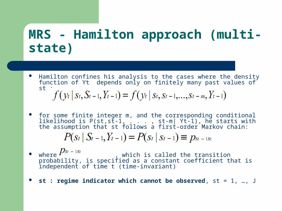
Hamilton confines his analysis to the cases where the density function of Yt depends only on finitely many past values of st :
for some finite integer m, and the corresponding conditional likelihood is P(st,st-1, . . . , st-m| Yt-1), he starts with the assumption that st follows a first-order Markov chain:
where , which is called the transition probability, is specified as a constant coefficient that is independent of time t (time-invariant)
st : regime indicator which cannot be observed, st = 1, …, J

MRS - Hamilton approach
The conditional likelihood P (st , . . . , st-m| Yt-1) can then be calculated iteratively through two equations as follows:

MRS - Hamilton approach
The term P (st-1, . . . , st-m-1| Yt-1), in which the first st-1 term and Yt-1are both subscripted by the same period of time, is then computed as follows:
for t = 1, 2, . . . , T . Given initial values P (s1, sо, s-1, . . . , s-(m-1)| Yо), we can calculate by iteration.

MRS - Filtering
Having P (st,st-1, . . . , st-m| Yt), we can eliminate the st,st-1, . . . , st-m terms as follows:
This is called the filtering probability. Basing on observation it can “filter out” the unobserved state of world.

MRS - Predicting
In the same way, we can also calculate all the predicting probability.The probability becomes predicting probability as we restrict r < t.
For instance, the one-step ahead predicting probability can be calculated by “integrating out” the st, st-1, . . . , st-m terms in
:

MRS - Smoothing
On the other hand, when r > t, we can have the so-called smoothed probability
This is for retrieving all the past states of the world. For example,
for j = 1, 2, …, m, can be easily calculated as :

MRS - Smoothing
A special smoothed probability which is based on all T observations of yt, can be calculated as (Hamilton, 1989) :
Where:

MRS – Data
data used for analyze is the BetFi index from the Bucharest Stock Exchange (BSE) at weekly frequency beginning with the starting date of this index (november 2000 ) and ending with end of june 2008
I also used for analyze a subsample from 2005 until 2008 to be able to catch the variability and the structure switching of the returns

MRS – The Matlab Program
The developed Matlab program is very flexible and the central point of this flexibility resides in the input argument S, which controls for where to include markov switching effect.
For instance, if you have 2 explanatory variables ( x1t , x2t ) and if the input argument S, which is passed to the fitting function MS_Regress_Fit.m, is equal to S=[1 1], then the model for the mean equation is:
Where: represents the state at time t, that is, St = 1 … K , where K is the number of states is the model’s standard deviation at state St is the beta coefficient for explanatory variable i at state St where i goes from 1 to n
is the residue which follows a particular distribution (in this case Normal or Student)

MRS – The Matlab Program

RMS - results 2000-2008


RMS - results 2005-2008


MRS – results table
Period 2000 – 2008 :
Period 2005 – 2008 :
Variables Distribution assumption
Method for calculati
ng σ
Model State 1 Model State 2 Xt ,State 1 Xt ,State 2 Transition Probability
Matrixσ ε σ ε Value ε Value ε
Yt = BetFi ReturnXt=Constant
Normal White 0.023268
0.0046151
0.010276
0.0057572
0.0070394
0.0026286
0.005598
0.0019898
P11 = 0.947P12 =0.135P21 =0.052 P22 =0.864
T ratio – 5.042 T ratio – 1.785 T ratio – 2.678 T ratio – 2.813
Variables Distribution assumption
Method for calculati
ng σ
Model ,State 1 Model ,State 2 Xt ,State 1 Xt ,State 2 Transition Probability
Matrixσ ε σ ε Value ε Value ε
Yt = BetFi ReturnXt=Constant
Normal Newey West
0.017912
0.0046066
0.044474
0.015899
0.0022364
0.00089592
0.0030684
0.001375
P11 = 0.953P12 =0.224P21 =0.046 P22 =0.775
T ratio – 3.888 T ratio – 2.798 T ratio – 2.496 T ratio – 2.232

Present Value Model - Data
the returns used in the model estimation are constructed at trimester frequency beginning with 2000:02 and ending with 2007:04 as follows:
BetFi returns – taking into account that this index has components formed by 5 financial investments companies and the starting date of existing was november 2000, I estimate the returns from the period april 2000 until november 2000, folowing the structure of this index; Source: BSE
Short rate returns – I calculate the short rate return, following the formula: (Bubid+Bubor)/2, where Bubid and Bubor were considered on a horizon of 3 months; Source: National Bank of Romania (NBR)
Dividend returns – I calculate the dividend on index following the structure and the percentage of the each company in the index. To obtain trimester data, i interpolate the values between two consecutive years. The type of the function that I used for interpolation is cubic spline data interpolation ; Source: BSE
Consumer Price Index – source: National Institute of Statistics

Present Value Model – results comparison
Present Value Model - Comments
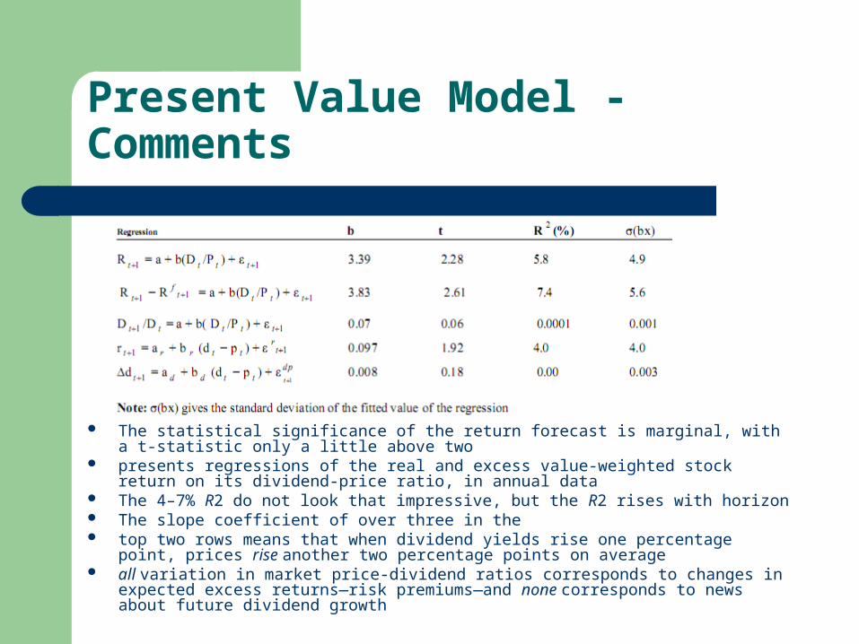
The statistical significance of the return forecast is marginal, with a t-statistic only a little above two
presents regressions of the real and excess value-weighted stock return on its dividend-price ratio, in annual data
The 4–7% R2 do not look that impressive, but the R2 rises with horizon The slope coefficient of over three in the top two rows means that when dividend yields rise one percentage point, prices rise
another two percentage points on average all variation in market price-dividend ratios corresponds to changes in expected excess
returns—risk premiums—and none corresponds to news about future dividend growth