stock options and credit default swaps: a joint framework for

Stock Options and Credit Default Swaps:

A Joint Framework for Valuation and Estimation

ABSTRACT

We propose a dynamically consistent framework that allows joint valuation and estimation of stock

options and credit default swaps written on the same reference company. We model default as controlled

by a Poisson process with a stochastic default arrival rate.When default occurs, the stock price drops

to zero. Prior to default, the stock price follows a continuous process with stochastic volatility. The

instantaneous default rate and instantaneous diffusion variance rate follow a bivariate continuous Markov

process, with its dynamics specified to capture the empirical evidence on stock option prices and credit

default swap spreads. Under this joint specification, we derive tractable pricing solutions for stock

options and credit default swaps. We estimate the joint dynamics using stock option prices and credit

default swap spreads for four of the most actively traded reference companies. Our estimation shows

that for all four reference companies, the default rate is much more persistent than the diffusion variance

rate under both the time series measure and the risk-neutralmeasure. Furthermore, changes in diffusion

variance are positively related to contemporaneous and subsequent changes in the default rate. Finally,

the estimation reveals that the market price of default arrival risk is negative while the market price of

diffusion variance risk is positive, suggesting that for individual stocks, shorting credit default swaps

generates a higher average return per unit risk than shorting variance swap contracts.

JEL Classification:C13; C51; G12; G13.

Keywords:Stock options; credit default swaps; default arrival rate; return variance dynamics; option pricing;

time-changed Levy processes.

2

Stock Options and Credit Default Swaps:

A Joint Framework for Valuation and Estimation

Markets for both stock options and credit derivatives have experienced dramatic growth in the past few

years. Along with the rapid growth, it has become increasingly clear to market participants that stock option

implied volatilities and credit default swap spreads are inherently linked. Many academic studies have

also empirically documented the positive link between credit spreads and stock volatility at both the firm

level and the aggregate level.1 Interestingly, this empirical relationship has been presaged by classical asset

pricing theory. According to the classic structural model of Merton (1974), corporate bond credit spreads are

functions of financial leverage and firm asset volatility, both of which have positive impacts on the volatility

of the underlying company’s stock and hence on stock option implied volatilities.

Furthermore, when a company defaults, the company’s stock price inevitably drops by a sizeable amount.

As a result, the possibility of default on a corporate bond generates negative skewness in the probability dis-

tribution of stock returns. This negative skewness is manifested in the relative pricing of stock options across

different strikes. When the Black and Scholes (1973) implied volatility is plottedagainst some measure of

moneyness at a fixed maturity, the average slope of the plot is positively related to the risk-neutral skewness

of the stock return distribution. Dennis and Mayhew (2002) and Bakshi, Kapadia, and Madan (2003) exam-

ine the negative skew of the implied volatility plot for individual stock options. Recent empirical work, e.g.,

Cremers, Driessen, Maenhout, and Weinbaum (2004), shows that credit default swap rates are positively

correlated with both stock option implied volatility levels and the steepness of the negative slope of the

implied volatility plot against moneyness.

In this paper, we propose a dynamically consistent framework that allows joint valuation and estimation

of stock options and credit default swaps written on the same reference company. We model company default

as controlled by a Poisson process with a stochastic arrival rate. When default occurs, we let the stock price

drop to zero. Prior to default, we model the stock price by a continuous process with stochastic volatility. The

1Examples include Bevan and Garzarelli (2000), Pedrosa and Roll (1998), Collin-Dufresne, Goldstein, and Martin (2001),

Bangia, Diebold, Kronimus, Schagen, and Schuermann (2002), Capmbell and Taksler (2003), Altman, Brady, Resti, and Sironi

(2004), Bakshi, Madan, and Zhang (2004), Ericsson, Jacobs, and Oviedo-Helfenberger (2004), Hilscher (2004), Consigli (2004),

and Zhu, Zhang, and Zhou (2005).

instantaneous default rate and instantaneous diffusion variance rate follow a bivariate continuous Markov

process, with its joint dynamics specified to capture the empirical evidence onstock option prices and credit

default swap spreads.

Under this joint specification, we derive tractable pricing solutions for stock options and credit default

swaps. We then estimate the joint dynamics of default rate and diffusion variance rate using stock option

prices and credit default swap spreads for four of the most actively traded reference companies. Our es-

timation shows that for all four reference companies, the default rate is more persistent than the diffusion

variance rate under both the time-series and the risk-neutral measures. Furthermore, changes in diffusion

variance are positively related to contemporaneous and subsequent changes in the default rate. Finally, com-

paring the time-series and risk-neutral dynamics reveals that the market price of the default arrival rate risk

is negative, but the market price for diffusion variance risk is positive.Previous works such as Bakshi and

Kapadia (2003) and Carr and Wu (2004b) have studied the market priceof aggregate variance risk and have

found that at least for stock indexes, the risk premia are negative. Ourresults in this paper suggest that for

individual stocks, negative variance risk premia are mainly due to the variance risk generated from down-

side jumps. From a practical perspective, a negative aggregate variance risk premium suggests that selling

variance swap contracts generates positive average returns. The negative default risk premium versus the

positive diffusion variance risk premium on the four stocks further suggest that selling credit insurance using

credit default swap contracts generates an even higher rate of average return per unit risk.

The positive empirical relation between credit default swap spreads andstock option implied volatilities

has been recognized only very recently in the academic community. As a result, efforts to theoretically

capture this link are only in an embryonic stage. In a recent working paper, Hull, Nelken, and White (2004)

link credit default swap spreads and stock option prices by proposing anew implementation and estimation

method for the classic structural model of Merton (1974). As it is well known, this early model is highly

stylized as it assumes that the only source of uncertainty is the firm’s asset value. As a result, stock option

prices and credit default swap spreads have changes that are perfectly correlated locally. Thus, the empirical

observation that implied volatilities and swap spreads sometimes move in opposite directions can only be

accommodated by adding additional sources of uncertainty to the model.

2

In this paper, we assume that prior to default, the stock price process is continuous. Both the drift and

diffusion of this process are stochastic as we assume that the default arrival rate and diffusion variance rate

obey a bivariate dynamic process. As a result, we are able to capture the imperfect positive correlation

between stock volatility and default risk. Thus, when compared to efforts based on the structural model of

Merton (1974), our contribution amounts to adding consistent and interrelated but separate dynamics to the

relation between volatility and default. This separation of the two sources of risk allows us to estimate and

compare the market prices of these risks, a feat that cannot possibly beachieved by daily static calibration of

simpler models. The dynamic consistency embedded in our specification and estimation is important, as it

provides a stable framework for dynamic hedging and integrated investmentacross the two markets. It also

generates insights on how different sources of risks are priced and how they affect the dynamics of credit

spreads and option prices differently.

The rest of the paper is organized as follows. The next section proposes a joint valuation framework for

stock options and credit default swaps. Section 2 describes the data setand summarizes the stylized evidence

that motivates our specification. Section 3 describes the joint estimation procedure. Section 4 presents the

results and discusses their implications. Section 5 concludes.

1. Joint Valuation of Stock Options and Credit Default Swaps

Consider a reference company that has a positive probability of defaulting. Let λ(t) denote the arrival rate

of the default event, which we allow stochastic. LetPt denote the time-t stock price for this company, which

we assume falls to zero upon default. Let(Ω,F ,(F t)t≥0,Q) be a complete stochastic basis andQ be a

risk-neutral probability measure, under which the stock price dynamicsprior to company defaultfollows:

dPt/Pt = (r (t)−q(t)+λ(t))dt+√

v(t)dWst , (1)

wherer (t) andq(t) denote the instantaneous interest rate and dividend yield, respectively,which we assume

deterministic,Wst denotes a standard Brownian motion, andv(t) denotes the instantaneous variance rate for

the stock diffusion return component, which we also allow stochastic. The incorporation ofλ(t) in the drift

compensates for the possibility of a default, so that the stock price remains a martingale unconditionally

3

under the risk-neutral measure. Thus, both the drift and the diffusion of this pre-default stock price process

are stochastic.

1.1. Joint dynamics of diffusion variance rate and default arrival rate

We model the joint dynamics of the default arrival rate and the diffusion return variance rate under the

risk-neutral probability measureQ as follows:

dv(t) = (θv−κvv(t))dt+σv

√v(t)dWv

t , (2)

dz(t) = (θz−κzz(t)−κzvv(t))dt+σz

√z(t)dWz

t , (3)

λ(t) = z(t)+ξv(t), (4)

ρsv ≡ E [dWsdWv]/dt < 0, ρsz≡ E [dWsdWz] = 0, ρzv≡ E [dWzdWv] = 0. (5)

The specifications are motivated by both empirical evidence and economic rationale:

• Cremers, Driessen, Maenhout, and Weinbaum (2004) find that option volatility predict credit default

swap spreads. Our own empirical analysis finds similar evidence. Equation(3) captures this pre-

dictability via the cross drift term,κzvv(t). A negative estimate forκzv would indicate that diffusion

return variancevt positively predicts changes in the risk factorz(t), which feeds directly into the

default arrival rateλ(t) via equation (4).

• Anecdotal evidence shows that when concerns of default arise for acompany, the stock price for that

company often becomes more volatile due to market “jitters.” Our empirical analysis also reveals

positive contemporaneous correlation between daily changes in option impliedvolatility and credit

default swap spreads. Equation (4) captures the positive contemporaneous correlation via a positive

loading coefficient estimateξ between the default arrival rateλ(t) and the diffusion return variance

ratev(t).

• When stock price falls, its return volatility often increases. A traditional explanation that dates back

to Black (1976) for this well-documented phenomenon is the leverage effect. Falling stock price

4

increases the company’s leverage and hence its risk, which shows up in stock return volatility.2 Equa-

tion (5) captures this phenomenon via a negative correlation coefficientρsv between diffusion shocks

in return and return variance. Furthermore, this increased volatility also raises the default arrival rate

both contemporaneously via equation (4) withξ > 0 and subsequently via equation (3) withκzv < 0.

We assumeρsz= ρzv = 0 for parsimony and tractability.

In matrix notation, we can write the bivariate process as

dxt = (θ−κxt)dt+√

βxtdWt , (6)

with

xt =

vt

zt

, κ =

κv 0

κzv κz

, θ =

θv

θz

, β =

σ2v 0

0 σ2z

, Wt =

Wvt

Wzt

. (7)

1.2. Pricing stock options

Consider a claim that pays offV (PT) at expiryT if the company does not default before expiry andϖ at the

time of default any time before expiry. The valuation of such a contingent claim can be written as,

V (Pt ,K,T) = Et

[exp

(−Z T

t(r (s)+λ(s))ds

)V (PT)

]

+Et

[ϖZ T

tλ(s)exp

(−Z s

t(r (u)+λ(u))du

)ds

], (8)

where the expectation operatorEt [·] is under the risk-neutral measureQ and conditional on the filtrationF t .

2Various other explanations have also been proposed in the literature, e.g., Haugen, Talmor, and Torous (1991), Campbell and

Hentschel (1992), Campbell and Kyle (1993), and Bekaert and Wu (2000).

5

Now consider the value of a European call optionc(Pt ,K,T) as an example. The terminal payoff is

(PT −K)+ at maturityT if the company has not defaulted yet by that time. The payoff is zero otherwise.

The valuation becomes:

c(Pt ,K,T) = Et

[exp

(−Z T

t(r (s)+λ(s))ds

)(PT −K)+

]

= B(t,T)Et

[exp

(−Z T

tλ(s)ds

)(PT −K)+

], (9)

whereB(t,T) is the time-t discount factor with maturity dateT and the expectation can be solved by invert-

ing the following discounted generalized Fourier transform,

φ(u) ≡ Et

[exp

(−Z T

tλ(s)ds

)eiu lnPT/Pt

], u∈ D ⊂ C, (10)

whereD denotes the subset of the complex plane under which the expectation is well-defined. Under our

dynamic specifications in equations (1) to (5), the Fourier transform is exponential affine in the bivariate

state vectorxt :

φ(u) = exp(

iu(r(t,T)−q(t,T))τ−a(τ)−b(τ)⊤ xt

), τ = T − t, (11)

wherer(t,T) andq(t,T) denote the continuously compounded spot interest rate and dividend yieldrate at

time t and maturity dateT, respectively, and the coefficients[a(τ),b(τ)] can be solved from the following

set of ordinary differential equations:

a′ (τ) = b(τ)⊤ θ,

b′ (τ) = b0− (κM)⊤b(τ)− 12β(b(τ)⊙b(τ)) ,

(12)

starting ata(0) = 0 andb(0) = 0, with⊙ denoting the Hadamard product, and

b0 =

(1− iu)ξ+ 12

(iu+u2

)

1− iu

, κM =

κv− iuσvρ 0

κzv κz

. (13)

Appendix A provides details of the derivation. The ordinary differentialequations can be solved readily

using standard numerical procedures. Givenφ(u), option prices can be obtained via fast Fourier inversion

(Carr and Wu (2004a)).

6

1.3. Pricing credit default swap spreads

For a credit default swap contract initiated at timet and with maturity dateT, we useS(t,T) to denote the

premium (the “spread”) paid by the buyer of default protection. With continuous payment assumption, the

present value of the premium leg of the contract is,

Premium(t,T) = Et

[S(t,T)

Z T

texp

(−Z s

t(r(u)+λ(u))du

)ds

]. (14)

Similarly, the present value of the protection leg of the contract is

Protection(t,T) = Et

[wZ T

tλ(s)exp

(−Z s

t(r(u)+λ(u))du

)ds

], (15)

with (1−w) denoting the recovery rate. Hence, by setting the present values of the two legs equal, we can

solve for the credit default swap spread as

S(t,T) =Et

[wR T

t λ(s)exp(−R st (r(u)+λ(u))du)ds

]

Et

[R Tt exp(−R s

t (r(u)+λ(u))du)ds] , (16)

which can be regarded as a weighted average of the expected default loss. In model estimation, we discretize

the above equation according to quarterly premium payment intervals. We set the recovery rate fixed at 40

percent, the average recovery rate for senior unsecured debts andalso an industry standard number for credit

default swap valuation.

Under our default arrival dynamics specification in equations (2) to (5), we can solve the present values

of the two legs of the contract and hence the credit default swap spread. The value of the premium leg is

Premium(t,T) = S(t,T)Z T

tEt

[exp

(−Z s

t(r(u)+λ(u))du

)ds

]

= S(t,T)Z T

tB(t,s)Et

[exp

(−Z s

tb⊤λ0xudu

)]ds, (17)

7

with bλ0 = [ξ,1]⊤. The affine dynamics for the bivariate vectorx and the linear loading functionbλ0 dictate

that the present value of the premium leg is an exponential affine function of the state vector (Duffie, Pan,

and Singleton (2000)):

Premium(t,T) = S(t,T)Z T

tB(t,s)exp

(−aλ(s− t)−bλ(s− t)⊤xt

)ds, (18)

with

a′λ (τ) = bλ (τ)⊤ θ,

b′λ (τ) = bλ0−κ⊤bλ (τ)− 12β(bλ (τ)⊙bλ (τ)) ,

(19)

starting ataλ(0) = 0 andbλ(0) = 0.

Similarly, the present value of the protection leg is

Protection(t,T) = Et

[wZ T

tB(t,s)λ(s)exp

(−Z s

tλ(u)du

)ds

]

= wZ T

tB(t,s)Et

[(b⊤λ0xs

)exp

(−Z s

tb⊤λ0xudu

)]ds, (20)

which also falls into the affine structure and hence also has an exponentialaffine solution:

Protection(t,T) = wZ T

tB(t,s)

(c(s− t)+d(s− t)⊤xt

)exp

(−aλ (s− t)−bλ (s− t)⊤ xt

)ds, (21)

where the coefficients(aλ(τ),bλ(τ)) are the same as in (19), and the coefficients(c(τ),d(τ)) can be solved

from the following set of ordinary differential equations:

c′ (τ) = d(τ)⊤ θ,

d′ (τ) = −κ⊤d(τ)−β(bλ (τ)⊙d(τ)) ,(22)

starting atc(0) = 0 andd(0) = bλ0. Combining the solutions for the present values of the two legs in

equations (17) and (21) solves for the credit default swap spreadS(t,T).

8

1.4. Market prices of risks and time-series dynamics

Our joint estimation identifies both the time-series dynamics and the risk-neutral dynamics of the bivariate

state vectorxt . To derive the time-series dynamics for the bivariate vectorxt under the statistical measure

P, we assume that the market prices of risks are proportional to the risk level, γ√xt , with γ being a diagonal

matrix. Under this assumption, the time-series dynamics are,

dxt =(

θ−κPxt

)dt+

√βxtdWP

t , (23)

with κP = κ−√

βγ, and

γ =

γv 0

0 γz

. (24)

2. Data and Evidence

Both the stock option prices and the credit default swap spreads are functions of the bivariate vectorx(t) =

[v(t;z(t)], which jointly determines the stock diffusion variance and the default arrival rate. Therefore, we

can use data on stock option prices and credit default swap spreads to infer the joint dynamics.

2.1. Data description

We estimate the model using credit default swap spreads and stock options on four reference companies.

Bloomberg provides the credit default swap spreads quotes from several broker dealers. We use the quotes

from different broker dealers for cross-validation. Then, we take the quotes on each series from the most

reliable sources. We choose four companies under which the credit default swap quotes have both a long

history and frequent updates. The four companies are: Ford (F), General Motors (GM), Altria Group Inc

(MO), and Duke Energy Corp (DUK). For each company, we have credit default swap spread series at five

fixed maturities of one, three, five, seven, and ten years.

The corresponding stock options data are from OptionMetrics. Exchange-traded options on individual

stocks are American style and hence the price contains an early exercise premium. OptionMetrics uses

9

a binomial tree approach to back out the option implied volatility that explicitly accounts for the early

exercise premium. We directly use the implied volatility from OptionMetrics. For model estimation, we

convert the implied volatility into European option prices using the Black-Scholes formula. For each stock,

the OptionMetrics provides a standardized implied volatility surface at fixed Black-Scholes forward deltas

from 20 to 80 with a five-delta interval for both call and put options, and fixed option maturities of 30,

60, and 91 days. OptionMetrics estimates the implied volatility surface via a kernel smoothing approach

whenever the underlying quotes are available and left as missing values when there are not enough quotes to

make the smoothing estimation. Data at longer maturities are also available but only very sparsely. Hence

we only use the first three maturities. No-arbitrage dictates that the implied volatilitycomputed from put

and call option prices at the same strike should be the same. Nevertheless, the implied volatility estimates

from OptionMetrics are often different from calls and puts at similar strikes, possibly resulting from bid-ask

spreads, misalignments of interest rates and dividend yields, and/or errors induced by the smoothing method

and the binomial tree approach in obtaining implied volatilities. For estimation, we takethe average of the

two implied volatility at each strike and convert them into out-of-money option prices.

To price the credit default swap contracts and to convert the implied volatility into option prices, we

also need the underlying interest rate curve. Following standard practicein the industry, we use the interest

rate curve defined by the eurodollar libor and swap rates. We download libor rates at maturities of one,

two, three, six, nine, and 12 months and swap rates at two, three, four, five, seven, and ten years. We use a

piece-wise constant forward function in bootstrapping the discount ratecurve.

2.2. Summary statistics

Model estimation uses the common samples of the three data sets that from January 2, 2002 to April 30,

2004. The data are available in daily frequency, but we estimate the model using weekly-sampled data on

every Wednesday to avoid the impacts of weekday effects. Table 1 reports the summary statistics of the

credit default swap spreads on the four reference companies. The mean term structures of the spreads are

relatively flat for all four companies, but the standard deviations of the spreads for all four companies decline

with increasing maturities. The weekly autocorrelation estimates for the spreads range from 0.90 to 0.97,

showing that the swap spreads and hence the default arrival rate dynamics are highly persistent.

10

Table 2 reports the summary statistics of stock option implied volatilities at the three fixed maturities

and 13 fixed put-option deltas for each of the four reference companies. For each company and at each

option maturity, the implied volatilities at low strikes (low put deltas) are on averagehigher than the implied

volatilities at high strikes, generating a negatively sloped average implied volatility smirk across money-

ness. The standard deviations of the implied volatility series are also larger for out-of-money puts than for

out-of-money calls, but the difference is smaller than the difference in the mean estimates. The weekly

autocorrelation for the volatility series range from 0.69 to 0.93, indicating thatthe implied volatilities are

persistent, but less so than the credit default swap spreads.

Figure 1 plots the average implied volatility smirk at the three fixed maturities as a function of the

put option delta. For all the four reference companies and under all three fixed maturities, the average

implied volatility smirk is negatively skewed, corresponding to a negatively skewed risk-neutral stock return

distribution. The three lines in each panel, which correspond to the three option maturities, stay closely to

one another, suggesting that the conditional risk-neutral distribution of the stock return retains similar shapes

at the three conditioning horizons. Generically, our model specification can generate the negative skewness

from two sources: (1) a positive probability of default (λ(t) > 0) and (2) a negative correlation between the

return Brownian motion component and its instantaneous variance rate (ρsv < 0).

[Figure 1 about here.]

2.3. Co-movements between option implied volatilities andcredit default swap spreads

Figure 2 overlays the daily time series of the credit default swap spreads (solid lines) with the daily time

series of at-the-money (50 delta) stock option implied volatilities at the three fixedoption maturities (dashed

lines) for the four chosen reference companies. We observe apparent common movements for two types of

time series for each company. The co-movements are the most obvious duringfinancial distresses for the

company, during which the two sets of time series both spike up.


11

To quantify the co-movements, we choose the five-year credit default swap spread series (St) and the

three-month 50-delta implied volatility series (ATMVt) and run the following regression on the daily series:

St = a+bATMVt +et . (25)

Table 3 reports the parameter estimates,t-statistics, andR2 of the regression for each of the four reference

companies. Figure 3 shows the corresponding scatter plots and fitted lines.The significantly positive slope

estimates confirm the positive co-movements between the two series. Nevertheless, we also observe that the

R2 estimates of the regressions vary significantly across different reference companies. The estimates are

largest at 82 percent for Ford, and lowest at only 36 percent for Altria Group. The variations across different

companies and the lowR2 estimates in some instances suggest that although return variance and default

arrival share common movements, they also have their own independent movements. The relative strength

of co-movements may vary across different reference companies.3 From the modeling perspective, it is

important to capture not only the common movements between the two markets but also the idiosyncratic

movements in each market. Our bivariate risk dynamics in equations (2) to (5) can accommodate different

degrees of common and idiosyncratic movements.


Given the high persistence for both credit swaps spreads and implied volatilities, we also study how the

daily changes of one series is correlated with the daily changes of anotherseries. Figure 4 plots the cross-

correlograms at different leads and lags between daily changes in the five-year credit default swap spread and

the three-month at-the-money implied volatility. The dash-dotted lines in each panel denote the 95 percent

confidence band. For all four reference companies, we identify significantly positive contemporaneous

correlations between the daily changes of the two series. Nevertheless, the correlation estimates are all

below 0.5, indicating again that the two markets both share common movements and possess independent

characteristics.

3Using other maturities for the two series generate similar results that are available upon request.

12

Furthermore, for all four companies, lagged values (up to a week) of theat-the-money implied volatilities

significantly and positively predict movements in the credit default swap spreads. One potential reason for

this predictability is the liquidity difference between the two markets. The stock options are exchange-

listed. The quotes are possibly updated more frequently than the over-the-counter quotes on the credit

default swap spreads. Irrespective of the underlying source, ourdynamic specification captures both the

positive contemporaneous correlation via a positive loading coefficientξ and the predictive relation via a

negative value forκzv.


3. Joint Estimation of Return Variance and Default Arrival Dynamics

We estimate the bivariate risk dynamics jointly using both credit default swap spreads and stock options. We

cast the model into a state-space form and estimate the model using the quasi-maximum likelihood method.

In the state-space form, we regard the bivariate risk vector as the unobservable states and specify the

state propagation equation using an Euler approximation of the time-series dynamics in equation (23):

xt = θ∆t +ϕvt−1 +√

βvt−1∆tεt , (26)

whereϕ = exp(−κP∆t) denotes the autocorrelation coefficient with∆t being the length of the discrete time

interval, andε denotes an iid bivariate standard normal innovation. We sample the data weekly for the

estimation, hence∆t = 7/365. The conditional covariance matrix of the state vector is a diagonal matrix

with state-dependent diagonal elements:

Q t = diag〈βvt−1∆t〉,

wherediag〈·〉 denotes a diagonal matrix with the diagonal elements given by the vector insidethe bracket.

13

We construct the measurement equations based on credit default swap spreads and stock options, assum-

ing additive, normally-distributed measurement errors:

yt = h(xt ;Θ)+et , (27)

whereyt denotes the observed series andh(xt ;Θ) denotes the corresponding model value as a function of the

state vectorxt and model parametersΘ. Specifically, the measurement equation contains five default credit

swap spread series and 39 option series,

h(xt ;Θ) =

S(xt , t + τs;Θ)

O(xt , t + τO,δ;Θ)

,τs = 1,3,5,7,10 years

τO = 30,60,91 days;δ = 20,25, · · · ,80,(28)

whereS(xt , t + τs) denotes the model value of the credit default swap spreads at timet and maturityτs as a

function of the state vectorxt and model parametersΘ, O(xt , t + τO,δ;Θ) denotes the model value for out-

of-money options at timet, time-to-maturityτO, and deltaδ, as a function of the state vectorxt and model

parametersΘ. We scale the out-of-money option prices by their Black-Scholes vega. There are missing

values on both the credit swap data and the implied volatility surface. Our estimation algorithm readily

handles missing observations. The termet in (27) denotes the measurement errors, with its covariance

matrix R . We assume that the five credit default spread series generate iid normalpricing errors with the

same error varianceσ2s. We also assume that the pricing errors on all the options (scaled by their vega) are

also iid normal with error varianceσ2O.

For model estimation, letxt ,Vt ,yt ,At denote the time-(t−1) ex ante forecasts of time-t values of the state

vector, the covariance of the state vector, the measurement series, and the covariance of the measurement

series, respectively, and letxt andVt denote the ex post updates on the state vector and its covariance at

the timet based on observations (yt) at timet. The state-propagation equation is Gaussian-linear, but the

measurement equation in (27) is nonlinear. We use the unscented Kalman filterto handle the nonlinearity.

The filter uses a set of deterministically chosen points to match not only the mean and variance, but also the

higher moments of the state distribution.

14

Let k = 2 denote the number of states and letζ > 0 denote a control parameter, a set of 2k+ 1 sigma

vectorsχi are generated according to the following equations,

χt,0 = xt ,

χt,i = xt ±√

(k+ζ)(Vt +Q t) j , j = 1, · · · ,k; i = 1, · · · ,2k,

with the corresponding weightswi given by,

w0 = δ/(k+ζ), wi = 1/[2(k+ζ)], i = 1, · · · ,2k.

These sigma vectors form a discrete distribution withwi being the corresponding probabilities, such that the

mean, covariance, skewness, and kurtosis of this distribution arext , Vt +Q t , 0, andk+ζ, respectively.

Given the sigma points, the prediction steps are given by:

χt,i = θ∆t +ϕχt,i ;

xt+1 =2k

∑i=0

wi(χt,i);

Vt+1 =2k

∑i=0

wi(χt,i −xt+1)(χt,i −xt+1)⊤; (29)

yt+1 =2k

∑i=0

wih(χt,i

);

At+1 =2k

∑i=0

wi[h(χt,i

)−yt+1

][h(χt,i

)−yt+1

]⊤+R ,

and the filtering updates are given by

xt+1 = xt+1 +Kt+1(yt+1−yt+1) ;

Vt+1 = Vt+1−Kt+1At+1K⊤t+1, (30)

with

Kt+1 = St+1(At+1

)−1; St+1 =

2k

∑i=0

wi[χt,i −vt+1

][h(χt,i

)−yt+1

]⊤.

We refer to Julier and Uhlmann (1997) for general treatments of the unscented Kalman filter.

15

Based on the predicted mean and covariance on the observations, we construct the weekly log-likelihood

function assuming normally distributed forecasting errors,

lt+1(Θ) = −12

log∣∣At

∣∣− 12

((yt+1−yt+1)

⊤ (At+1

)−1(yt+1−yt+1)

). (31)

Then, the model parameters are chosen to maximize the log likelihood of the data series, which is a summa-

tion of the weekly log likelihood values,

Θ ≡ argmaxΘL (Θ,ytN

t=1), with L (Θ,ytNt=1) =

N−1

∑t=0

lt+1(Θ), (32)

whereN denotes the number of weeks in our sample. The procedure estimates 13 model parameters:

Θ ≡ [κv,κz,κP

v ,κP

z ,θv,θz,σv,σz,ξ,κzv,ρsv,σ2s,σ

2O]⊤. (33)

4. Joint Dynamics and Pricing of Return Variance and Default Arrival Risks

First, we summarize the performance of our joint valuation model on credit default swap spreads and stock

options on the four reference companies. Then, from the structural parameter estimates we discuss the joint

dynamics and pricing of the diffusion variance risk and default arrivalrisk.

4.1. Performance analysis

Table 4 reports the explained variation and predicted variation for the 39 option series for each company.

The explained variation is a measure of pricing performance, defined as one minus the sample variance of

the pricing erroret over the sample variance of the original seriesyt . It is analogous to anR2 measure for

a nonlinear regression. The model’s pricing performance on stock options is relatively uniform across all

four companies. The explained variations are over 90 percent for near the money options across all stocks.

The performance remains reasonably well for out-of-money put options, but become significantly worse

for out-of-money call options (high put delta). In the stock options market,out-of-money put options are

more actively traded than out-of-money call options. The quotes on the out-of-money put options are also

16

more reliable and consistent in general. On the other hand, the out-of-money call option prices often show

significant idiosyncratic variations. The model captures the behavior of out-of-money put options well.

The predicted variation is a measure of predictive performance, definedas one minus the sample vari-

ance of the predictive error over the sample variance of the original series. As expected, the predicted

variation is significantly smaller than the explained variation, suggesting that theoptions series contain a

significant portion of unpredictable movements. The decline is the most notablefor out-of-money call op-

tions. The predicted variation for some out-of-money call option series even become negative, suggesting

no predictability at all for these series.

To obtain a better picture on the pricing performance, we convert the model-implied option prices into

the Black-Scholes implied volatilities and redefine the pricing errors as the difference in percentage points

between the observed series and model values of the implied volatilities. Table 5reports the sample estimates

of the mean, standard deviation, and weekly autocorrelation of the pricing errors on implied volatilities. The

mean pricing errors are fairly small and show no obvious patterns acrossmoneyness and maturities. The

standard deviation ranges from one to four percentages points. Comparing these estimates to the mean im-

plied volatility estimates in Table 2 point to an average pricing error of less than ten percent. The weekly

autocorrelations of the pricing errors in implied volatilities are also much lower than the weekly autocorre-

lations of the original series.

Table 6 reports the explained variation and predicted variation for the five credit default swap spread

series for each of four reference companies. The model’s pricing performance is good for Ford and Duke

Energy, as the explained variations on all series are over 80 percent. However, the model performance is

relatively poor for General Motors, and even worse for Altria Group.The model explains less than 50

percent of variation for most of the series on these two companies.

Inspecting the time series plots in Figure 2, we observe that for General Motors, the five credit default

swap spread series diverge dramatically after January 2003 to generate a very steep term structure from a

virtually flat term structure before 2003. This dramatic term structure change either comes from economic

forces or from a mere fact of more frequent quote updating in the second half of the data. Irrespective of

the underlying reasons, our two-factor model seems to have difficulties fitting the whole term structure of

credit default swap spreads and the options data. The model performs well on all the options series, and

17

also reasonably well on short-term credit default swap spreads, butit performs poorly on the long-term

swap spreads. For Altria Group, the credit default swap data are not updated as frequently before 2003

whereas the options data are actively quoted and traded. It is potentially due to this difference that the model

parameters are geared to price the options market better than the credit default swap spreads.

Table 7 reports the sample estimates of the mean, standard deviation, and weekly autocorrelation of the

pricing errors on the credit default swap spreads in percentage points. Corresponding to the lower explained

variation, the standard deviations and weekly autocorrelations are relatively large for the pricing errors on

the credit spreads, especially for General Motors and Altria Group.

4.2. The joint dynamics of return variance and default arrival rates

Table 8 reports in panel A the maximum likelihood estimates andt-statistics of the structural parameters

that control the joint dynamics of the diffusion variance rate and the default arrival rate. The joint dynamics

differ across different companies. Nevertheless, several common features emerge from the estimates.

First, the estimates for the risk-neutral mean-reverting coefficients (κv,κz) and their time-series counter-

parts (κPv ,κP

z ) show that the default arrival rate is much more persistent than the diffusion variance rate under

both the risk-neutral measureQ and the time-series measureP. Their persistence difference is larger under

the risk-neutral measure.

The difference in statistical persistence suggests that the diffusion variance rates are strongly mean-

reverting and hence predictable, but that the default arrival rate is slow in reverting back to its long-run

mean level. The small estimates forκPz suggest that it is difficult to predict the default arrival changes based

on its past values as the movements of the default risk factorz are close to that of a random walk.

The difference in risk-neutral persistence indicates that the two factors(vt ,zt) have different loading pat-

terns across the term structure of options and credit default swap spreads. Shocks on the diffusion variance

rate affect the short-term options and credit default swap spreads, but dissipate quickly as the option and

swap maturity increases. In contrast, shocks on the more persistent default arrival rate last longer across the

term structure of options and credit spreads.

18

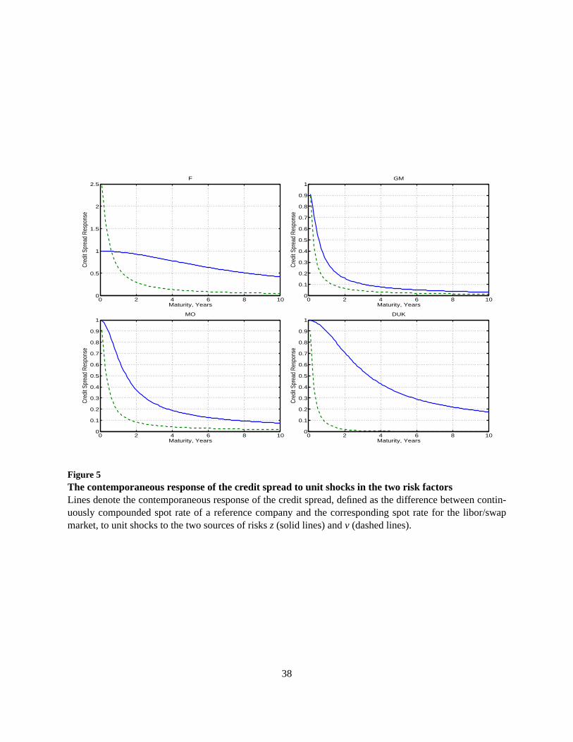
If we define the credit spread at a maturityτ as the difference between the continuously compounded

spot rate on a reference company and the corresponding spot rate in the benchmark eurodollar market, under

our dynamic model specification this spread is affine in the state vector,

Spread(t,τ) =

[aλ(τ)

τ

]+

[bλ(τ)

τ

]⊤xt , (34)

with the coefficients[aλ(τ),bλ(τ)] given by the ordinary differential equations in (19). Hence,bλ(τ)/τ

measures the contemporaneous response of the credit spread term structure to unit shocks on the two risk

factors. Figure 5 plots this response as a function of the credit spread maturity. The solid lines denote the

response to the default risk factorz whereas the dashed lines denote the response to the diffusion variance

factorv. The higher persistence inz dictates that its impact declines more slowly as maturity increases than

the impact of the more transient factorv.


The second common feature for the four reference companies is on how the default arrival rate interacts

dynamically with the return variance rate. The estimates for the loading coefficient ξ are positive for all

four companies, suggesting that positive shocks on the return variancerate increase the default arrival rate

contemporaneously. The estimates for the cross termκzv are all negative, suggesting that the return variance

rate also positively predict default arrival rate movements. These estimates suggest positive co-movements

between stock option implied volatilities and credit default swap spreads.

Finally, for all four companies, the estimates for the instantaneous correlation between stock return and

return varianceρsv are negative, consistent with classic stories on the leverage effect.

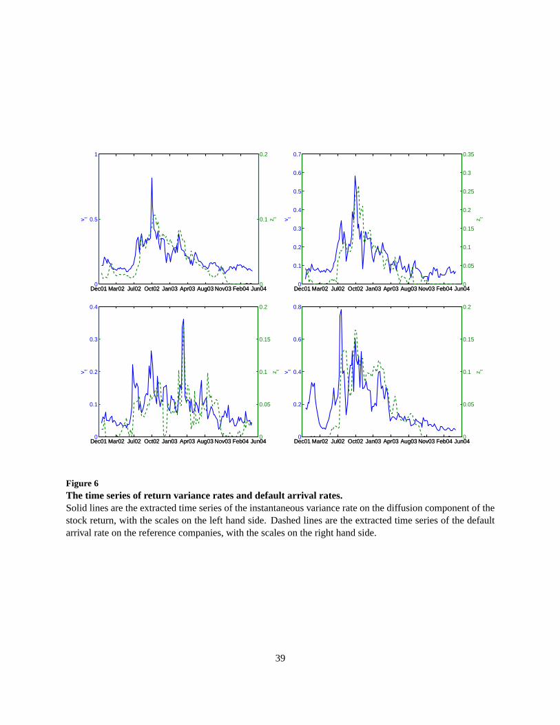
Figure 6 plots the extracted time series on the return variance rate (solid line) and the default arrival rate

(dashed line), with scales on the left and right hand sides of they-axis, respectively. The extracted time

series show common trends that match the time series plots of the credit default swap spreads and implied

volatilities in Figure 2. The plots for all four companies show a spike for both the variance rate and the

default arrival rate in late 2002, revealing the financial stress during that period.


19

4.3. Different market prices for diffusion variance risk and default arrival risk

The difference between the mean-reverting coefficients under the two measures defines the market prices

of the two sources of risks. Specifically, the market prices of diffusion return variance risk is given by

γv = (κv−κPv )/σv and the market price of the default risk factorz is given byγz = (κz−κP

z )/σz. Based on

the parameter estimates and covariance matrix, we compute the two market pricesfor each company and

report the estimates andt-statistics in panel B of Table 8. The estimates for all four companies show negative

market price for the default arrival rate risk, but positive market price for the diffusion variance risk.

The extant empirical studies, e.g., Bakshi and Kapadia (2003) and Carrand Wu (2004b), use stock and

stock index options and the underlying time series returns to study the total return variance risk premia. They

find that the risk premia are negative for some stocks, and highly negativefor stock indexes. Consistent with

the negative variance risk premia, selling options and delta hedge, or directly selling variance swap contracts,

generates positive average excess returns. Under our model specification, we decompose the total variance

risk into two components: risk in the default arrival rate and risk in the diffusion variance rate. By using

both the credit default swap data and stock options data, we are able to separate the two sources of risks and

identify their respective market prices. Our estimation suggests that for thefour stocks, negative variance

risk premia only come from the variance generated from negative jumps, not from the variance generated

from the diffusion component of the stock return. From an investment perspective, our results suggest that

selling credit insurance through the credit default swap market generates an even higher average return per

unit risk than selling variance swap contracts.

5. Summary and Conclusions

Based on documented evidence on the joint movements between credit default swap spreads and stock

option implied volatilities, we propose a dynamically consistent framework for thejoint valuation and es-

timation of stock options and credit default swaps written on the same reference company. We model the

company default by a Poisson process with stochastic arrival rate, andassume that the stock price falls to

zero upon default. We model the pre-default stock price as following a continuous process with stochastic

volatility. We assume that the default arrival rate and diffusion variance rate follow a bivariate process with

20

dynamic interactions that match the empirical evidence linking stock option implied volatilities and credit

default swap rates. Importantly, our dynamic specification allows both commonmovements and indepen-

dent characteristics between the two markets.

Under this joint specification, we derive tractable pricing solutions for stock options and credit default

swaps. We then estimate the joint dynamics of the diffusion variance rate and the default arrival rate using

data on stock option implied volatilities and credit default swap rates for four of the most actively traded

reference companies. The estimation shows that the default arrival rateis much more persistent than the

diffusion variance rate under both the statistical measure and the risk-neutral measure. The statistical per-

sistence difference suggests different degrees of predictability. Therisk-neutral difference in persistence

suggests that the default arrival rate has a more long-lasting impact on theterm structure of option volatili-

ties and credit default swap spreads than does the diffusion variance.

The estimation also suggests that the diffusion variance feeds positively intothe hazard rate, both con-

temporaneously and dynamically. It is these positive dynamic interactions thatgenerate the observed co-

movements between credit default swap spreads and stock option implied volatilities.

Finally, comparing the parameter estimates that control the statistical and risk-neutral dynamics shows

that the market price for the default arrival risk is negative, but the market price for the diffusion variance

risk is positive, suggesting different prices for different sources of return variance risk.

21

Appendix. Generalized Fourier transform of stock returns

To derive the generalized Fourier transform:

φ(u) ≡ Et

[exp

(−Z T

tλ(s)ds

)eiu lnPT/Pt

], u∈ D ⊂ C, (A1)

we use the language of stochastic time change of Carr and Wu (2004a) and define

T t ≡Z T

tv(s)ds, T z

t ≡Z T

tz(s)ds, T λ

t ≡Z T

tλ(s)ds= T z

t +ξT t .

Then, conditional on no default during the time horizon[t,T], with τ = T − t, we can write the log stock return as

ln(PT/Pt) = (r(t,T)−q(t,T))τ+T λt +Ws

T t− 1

2T t , (A2)

wherer(t,T) andq(t,T) denote the continuously compounded spot interest rates anddividend yields of the relevant

maturity. The log return goes to negative infinite as the stock price falls to zero when default occurs.

The discounted generalized Fourier transform becomes

φ(u) = Et

[exp

(−T λ

t + iu(r(t,T)−q(t,T))τ+ iuT λt + iuWs

T t− 1

2iuT t

)]

= Et

[exp

(iuWsT t

+12

u2T t

)exp

(−T λ

t + iu(r(t,T)−q(t,T))τ+ iuT λt − 1

2iuT t −

12

u2T t

)]

= exp(iu(r(t,T)−q(t,T))τ)EM

t

[exp

(−(1− iu)T λ

t − 12

(iu+u2)T t

)]

= exp(iu(r(t,T)−q(t,T))τ)EM

t

[exp

(−(1− iu)T z

t −(

(1− iu)ξ+12

(iu+u2)

)T t

)],

where the new measureM is defined by

dM

dQ

∣∣∣∣t= exp

(iuWsT t

+12

u2T t

),

under which the drift of the two dynamic processes change to:

µM

v = θv−κvv(t)+ iuσvρsvv(t) ,

µM

z = θz−κzz(t)−κzvv(t)+ iuρszσz

√v(t)z(t).

22

Hence, by assumingρsz= 0, we maintain the affine structure forz(t) andv(t). Then, we have

φ(u) = exp(iu(r(t,T)−q(t,T))τ)EM

t

[exp

(−Z T

tb⊤0 xsds

)],

with

b0 =

(1− iu)ξ+ 12

(iu+u2

)

1− iu

,

dxt =(θ+κMxt

)dt+

√βxdWM,

κM =

κv− iuσvρ 0

κzv κz

.

We thus can derive the exponential affine solution accordingto Carr and Wu (2004a).

23

References

Altman, E. I., B. Brady, A. Resti, and A. Sironi, 2004, “The Link Between Default and Recovery Rates: Theory,

Empirical Evidence and Implications,”Journal of Business, forthcoming.

Bakshi, G., and N. Kapadia, 2003, “Delta-Hedged Gains and the Negative Market Volatility Risk Premium,”Review

of Financial Studies, 16(2), 527–566.

Bakshi, G., N. Kapadia, and D. Madan, 2003, “Stock Return Characteristics, Skew Laws, and the Differential Pricing

of Individual Equity Options,”Review of Financial Studies, 16(1), 101–143.

Bakshi, G., D. Madan, and F. Zhang, 2004, “Investigating theRole of Systematic and Firm-Specific Factors in Default

Risk: Lessons From Empirically Evaluating Credit Risk Models,” Journal of Business, forthcoming.

Bangia, A., F. X. Diebold, A. Kronimus, C. Schagen, and T. Schuermann, 2002, “Ratings Migration and the Business

Cycle, With Application to Credit Portfolio Stress Testing,” Journal of Banking and Finance, 26(2-3), 445–474.

Bekaert, G., and G. Wu, 2000, “Asymmetric Volatilities and Risk in Equity Markets,”Review of Financial Studies,

13(1), 1–42.

Bevan, A., and F. Garzarelli, 2000, “Corporate Bond Spreadsand the Business Cycle: Introducing GS-Spread,”Jour-

nal of Fixed Income, 9(4), 8–18.

Black, F., 1976, “The Pricing of Commodity Contracts,”Journal of Financial Economics, 3, 167–179.

Black, F., and M. Scholes, 1973, “The Pricing of Options and Corporate Liabilities,”Journal of Political Economy,

81, 637–654.

Campbell, J. Y., and L. Hentschel, 1992, “No News is Good News: An Asymmetric Model of Changing Volatility in

Stock Returns,”Review of Economic Studies, 31, 281–318.

Campbell, J. Y., and A. S. Kyle, 1993, “Smart Money, Noise Trading and Stock Price Behavior,”Review of Economic

Studies, 60(1), 1–34.

Capmbell, J. Y., and G. B. Taksler, 2003, “Equity Volatilityand Corporate Bond Yields,”Journal of Finance, 63(6),

2321–2349.

Carr, P., and L. Wu, 2004a, “Time-Changed Levy Processes and Option Pricing,”Journal of Financial Economics,

71(1), 113–141.

Carr, P., and L. Wu, 2004b, “Variance Risk Premia,” working paper, Bloomberg and Baruch College.

Collin-Dufresne, P., R. S. Goldstein, and J. S. Martin, 2001, “The Determinants of Credit Spread Changes,”Journal

of Finance, 56(6), 2177–2207.

24

Consigli, G., 2004, “Credit Default Swaps and Equity Volatility: Theoretical Modelling and Market Evidence,” work-

ing paper, University Ca’Foscari.

Cremers, M., J. Driessen, P. J. Maenhout, and D. Weinbaum, 2004, “Individual Stock Options and Credit Spreads,”

Yale ICF Working Paper 04-14, Yale School of Management.

Dennis, P., and S. Mayhew, 2002, “Risk-neutral Skewness: Evidence from Stock Options,”Journal of Financial and

Quantitative Analysis, 37(3), 471–493.

Duffie, D., J. Pan, and K. Singleton, 2000, “Transform Analysis and Asset Pricing for Affine Jump Diffusions,”

Econometrica, 68(6), 1343–1376.

Ericsson, J., K. Jacobs, and R. Oviedo-Helfenberger, 2004,“The Determinants of Credit Default Swap Premia,”

working paper, McGill University.

Haugen, R. A., E. Talmor, and W. N. Torous, 1991, “The Effect of Volatility Changes on the Level of Stock Prices and

Subsequent Expected Returns,”Journal of Finance, 46(3), 985–1007.

Hilscher, J., 2004, “Is the Corporate Bond Market Forward Looking?,” working paper, Harvard University.

Hull, J., I. Nelken, and A. White, 2004, “Mertons Model, Credit Risk and Volatility Skews,” working paper, University

of Toronto.

Julier, S. J., and J. K. Uhlmann, 1997, “A New Extension of theKalman filter to Nonlinear Systems,” working paper,

University of Oxford, Sydney, Australia.

Merton, R. C., 1974, “On the Pricing of Corporate Debt: The Risk Structure of Interest Rates,”Journal of Finance,

29(1), 449–470.

Pedrosa, M., and R. Roll, 1998, “Systematic Risk in Corporate Bond Yields,”Journal of Fixed Income, 8(1), 7–2.

Zhu, H., Y. Zhang, and H. Zhou, 2005, “Equity Volatility of Individual Firms and Credit Spreads,” working paper,

Bank for International Settlements.

25

Table 1Summary Statistics on credit default swap spreadsEntries report the sample estimates of the mean, standard deviation, and weekly autocorrelation on the creditdefault swap spreads (in percentages) at five fixed maturities for eachof the four reference companies. Thestatistics are based on weekly sampled data from January 2, 2002 to April 28, 2004.

Maturity 1 3 5 7 10

Mean:F 2.19 2.89 2.97 2.95 2.87GM 1.51 2.03 2.19 2.28 2.15MO 1.79 1.78 1.75 1.69 1.79DUK 2.31 2.14 1.99 1.92 1.27

Standard Deviation:F 1.31 1.38 1.16 1.06 0.96GM 0.89 0.82 0.72 0.69 0.67MO 1.15 0.84 0.72 0.62 0.32DUK 1.93 1.60 1.31 1.17 0.31

Autocorrelation:F 0.97 0.97 0.96 0.95 0.95GM 0.96 0.95 0.94 0.92 0.93MO 0.91 0.92 0.92 0.90 0.94DUK 0.96 0.97 0.96 0.96 0.96

26

Table 2Summary statistics on stock option impled volatilitiesEntries report the sample estimates of the mean, standard deviation, and weekly autocorrelation on theimplied volatilities (in percentages) at 13 fixed deltas and three fixed maturities for four reference companies.The statistics are based on weekly sampled data from January 2, 2002 to April 28, 2004.

Delta 20 25 30 35 40 45 50 55 60 65 70 75 80

Mean:F 1m 50.07 49.09 48.02 46.82 45.84 44.74 43.68 43.12 42.52 42.25 41.95 41.98 42.28F 2m 50.49 48.87 47.45 46.18 45.19 44.14 43.19 42.62 42.13 41.63 41.45 41.47 41.67F 3m 49.98 47.97 46.64 45.46 44.53 43.61 42.73 42.14 41.46 40.93 40.63 40.46 40.53GM 1m 40.87 39.39 38.16 37.14 36.33 35.60 34.95 34.42 33.96 33.54 33.19 32.94 32.95GM 2m 41.45 39.92 38.64 37.49 36.51 35.70 34.97 34.35 33.81 33.29 32.81 32.41 32.17GM 3m 41.58 39.84 38.46 37.29 36.24 35.34 34.58 33.92 33.31 32.71 32.14 31.64 31.27MO 1m 33.73 32.07 30.84 29.89 29.24 28.69 28.36 28.06 27.74 27.50 27.42 27.55 28.07MO 2m 33.23 31.79 30.71 29.85 29.17 28.63 28.21 27.81 27.42 27.09 26.86 26.78 26.91MO 3m 33.09 31.78 30.80 29.97 29.25 28.63 28.12 27.66 27.24 26.85 26.50 26.23 26.04DUK 1m 46.40 44.28 42.65 41.37 39.94 38.66 37.67 37.04 36.56 36.12 35.94 35.79 36.14DUK 2m 46.09 43.96 42.26 40.85 39.48 38.22 37.25 36.58 35.94 35.30 34.69 34.30 34.38DUK 3m 44.97 43.08 41.42 39.94 38.65 37.39 36.42 35.70 34.92 34.17 33.46 32.97 32.80

Standard Deviation:F 1m 15.93 15.29 14.71 14.31 13.88 13.40 12.95 12.39 11.90 11.72 11.47 11.17 10.59F 2m 15.55 15.03 14.39 13.57 12.97 12.40 11.86 11.64 11.37 10.62 10.33 10.15 10.03F 3m 15.24 14.41 13.69 12.85 12.27 11.79 11.31 11.14 10.63 10.04 9.75 9.49 9.16GM 1m 15.37 14.64 13.95 13.39 12.86 12.23 11.68 11.26 10.83 10.39 10.00 9.61 9.20GM 2m 14.60 13.88 13.14 12.51 11.95 11.35 10.79 10.30 9.85 9.46 9.04 8.61 8.14GM 3m 13.97 13.16 12.37 11.68 11.08 10.51 9.98 9.49 9.05 8.63 8.20 7.76 7.29MO 1m 10.99 10.38 9.96 9.62 9.25 8.98 8.71 8.46 8.18 7.93 7.77 7.70 7.74MO 2m 9.65 9.10 8.71 8.39 8.07 7.82 7.60 7.36 7.12 6.95 6.81 6.66 6.52MO 3m 9.18 8.65 8.20 7.85 7.57 7.33 7.11 6.89 6.69 6.56 6.42 6.26 6.13DUK 1m 19.25 18.36 17.76 17.05 16.44 15.82 15.20 14.65 14.23 13.91 13.47 13.04 12.54DUK 2m 17.43 16.52 15.94 15.36 14.72 14.06 13.47 12.94 12.55 12.15 11.64 11.16 10.64DUK 3m 16.54 15.61 14.80 14.16 13.50 12.86 12.29 11.77 11.38 10.96 10.50 10.05 9.63

Autocorrelation:F 1m 0.83 0.86 0.87 0.89 0.87 0.84 0.84 0.85 0.84 0.85 0.85 0.850.87F 2m 0.89 0.87 0.88 0.91 0.88 0.86 0.87 0.86 0.88 0.90 0.91 0.910.90F 3m 0.93 0.91 0.91 0.94 0.91 0.89 0.89 0.89 0.91 0.93 0.92 0.910.91GM 1m 0.92 0.93 0.93 0.93 0.93 0.93 0.93 0.93 0.92 0.92 0.92 0.92 0.90GM 2m 0.95 0.95 0.95 0.95 0.95 0.95 0.95 0.95 0.95 0.94 0.94 0.93 0.92GM 3m 0.96 0.96 0.96 0.96 0.96 0.96 0.95 0.95 0.95 0.95 0.95 0.95 0.94MO 1m 0.78 0.78 0.79 0.80 0.81 0.82 0.82 0.81 0.81 0.81 0.80 0.76 0.69MO 2m 0.84 0.84 0.85 0.85 0.86 0.86 0.86 0.86 0.87 0.87 0.86 0.84 0.80MO 3m 0.87 0.88 0.88 0.88 0.89 0.89 0.89 0.89 0.89 0.89 0.89 0.89 0.88DUK 1m 0.90 0.90 0.90 0.89 0.90 0.90 0.91 0.91 0.90 0.90 0.89 0.89 0.88DUK 2m 0.93 0.93 0.93 0.92 0.92 0.93 0.93 0.92 0.92 0.91 0.91 0.91 0.91DUK 3m 0.95 0.94 0.94 0.94 0.94 0.94 0.93 0.93 0.93 0.93 0.93 0.93 0.93

27

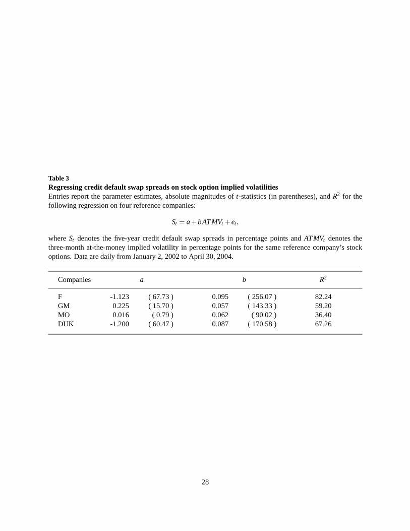
Table 3Regressing credit default swap spreads on stock option implied volatilitiesEntries report the parameter estimates, absolute magnitudes oft-statistics (in parentheses), andR2 for thefollowing regression on four reference companies:

St = a+bATMVt +et ,

whereSt denotes the five-year credit default swap spreads in percentage points andATMVt denotes thethree-month at-the-money implied volatility in percentage points for the same reference company’s stockoptions. Data are daily from January 2, 2002 to April 30, 2004.

Companies a b R2

F -1.123 ( 67.73 ) 0.095 ( 256.07 ) 82.24GM 0.225 ( 15.70 ) 0.057 ( 143.33 ) 59.20MO 0.016 ( 0.79 ) 0.062 ( 90.02 ) 36.40DUK -1.200 ( 60.47 ) 0.087 ( 170.58 ) 67.26

28

Table 4Explained and predicted variations on option pricesEntries in the first panel report explained variation on each option series, defined as one minus the variance ofthe pricing error over the variance of the original data series, and entries in the second panel report predictedvariation on each series, defined as one minus the variance of the predictive error over the variance of theoriginal series, at 13 fixed deltas and three fixed maturities for four reference companies. The statistics arebased on weekly sampled data from January 2, 2002 to April 28, 2004.

Delta 20 25 30 35 40 45 50 55 60 65 70 75 80

Explained Variation:F 1m 0.70 0.77 0.85 0.88 0.92 0.95 0.93 0.91 0.88 0.84 0.77 0.690.42F 2m 0.88 0.91 0.93 0.94 0.96 0.97 0.96 0.94 0.94 0.95 0.92 0.860.68F 3m 0.94 0.95 0.96 0.97 0.97 0.97 0.95 0.94 0.93 0.90 0.86 0.790.62GM 1m 0.94 0.96 0.97 0.98 0.99 0.99 0.99 0.98 0.98 0.96 0.94 0.88 0.69GM 2m 0.95 0.98 0.98 0.98 0.99 0.99 0.98 0.98 0.97 0.95 0.93 0.86 0.70GM 3m 0.96 0.99 0.99 0.99 0.99 0.99 0.98 0.97 0.96 0.94 0.90 0.80 0.55MO 1m 0.76 0.83 0.89 0.92 0.94 0.97 0.97 0.96 0.95 0.95 0.92 0.77 0.35MO 2m 0.90 0.94 0.95 0.97 0.97 0.98 0.97 0.96 0.93 0.91 0.86 0.75 0.47MO 3m 0.92 0.96 0.97 0.97 0.97 0.98 0.96 0.94 0.91 0.87 0.82 0.72 0.53DUK 1m 0.85 0.89 0.92 0.94 0.95 0.97 0.97 0.95 0.94 0.91 0.83 0.72 0.55DUK 2m 0.88 0.93 0.95 0.97 0.98 0.98 0.98 0.97 0.96 0.94 0.90 0.81 0.57DUK 3m 0.88 0.93 0.95 0.96 0.97 0.98 0.96 0.95 0.93 0.90 0.85 0.77 0.58

Predicted Variation:F 1m 0.12 0.36 0.54 0.65 0.71 0.76 0.64 0.46 0.24 0.04 -0.21 -0.55 -0.98F 2m 0.47 0.51 0.61 0.73 0.78 0.79 0.62 0.44 0.34 0.26 0.09 -0.20 -0.65F 3m 0.65 0.64 0.70 0.80 0.83 0.81 0.61 0.49 0.45 0.37 0.15 -0.18 -0.68GM 1m 0.38 0.49 0.58 0.66 0.73 0.80 0.73 0.62 0.46 0.25 -0.07 -0.57 -1.49GM 2m 0.59 0.67 0.73 0.78 0.82 0.86 0.77 0.68 0.56 0.40 0.14 -0.29 -1.07GM 3m 0.66 0.74 0.79 0.82 0.86 0.88 0.79 0.71 0.61 0.46 0.22 -0.19 -0.95MO 1m -0.32 -0.10 0.13 0.32 0.47 0.59 0.49 0.29 0.03 -0.32 -0.89 -1.79 -3.12MO 2m -0.11 0.10 0.28 0.44 0.56 0.66 0.51 0.33 0.09 -0.24 -0.73-1.50 -2.70MO 3m -0.13 0.14 0.32 0.47 0.59 0.69 0.55 0.38 0.16 -0.14 -0.57-1.21 -2.20DUK 1m 0.33 0.44 0.53 0.61 0.70 0.78 0.70 0.58 0.42 0.22 -0.09 -0.47 -1.01DUK 2m 0.50 0.59 0.66 0.71 0.78 0.83 0.72 0.59 0.42 0.22 -0.06 -0.48 -1.22DUK 3m 0.52 0.63 0.70 0.76 0.81 0.84 0.71 0.59 0.44 0.25 0.01 -0.34 -0.96

29

Table 5Summary statistics on the pricing errors in stock option impled volatilitiesEntries report the sample estimates of the mean, standard deviation, and weekly autocorrelation of thepricing errors in stock option implied volatilities, defined as the difference between observations and model-implied values in percentage points, at 13 fixed deltas and three fixed maturitiesfor four reference compa-nies. The statistics are based on weekly sampled data from January 2, 2002 to April 28, 2004.

Delta 20 25 30 35 40 45 50 55 60 65 70 75 80

Mean:F 1m -0.24 0.72 0.86 0.69 0.47 -0.04 -0.60 -1.10 -1.18 -1.24 -1.25 -1.03 -0.71F 2m -0.80 0.19 0.63 0.70 0.72 0.43 0.06 -0.07 -0.23 -0.53 -0.58 -0.53 -0.41F 3m -1.34 -0.32 0.45 0.82 1.06 1.01 0.78 0.68 0.33 0.01 -0.20 -0.39 -0.48GM 1m -0.02 0.39 0.47 0.44 0.37 0.25 0.12 0.02 -0.06 -0.13 -0.16 -0.11 0.19GM 2m -0.70 0.12 0.52 0.61 0.60 0.55 0.45 0.36 0.28 0.16 0.04 -0.03 0.03GM 3m -1.26 -0.37 0.10 0.28 0.28 0.20 0.11 0.00 -0.14 -0.33 -0.56 -0.76 -0.87MO 1m 0.79 0.51 0.22 -0.05 -0.18 -0.31 -0.29 -0.30 -0.38 -0.42-0.32 -0.04 0.57MO 2m -0.52 -0.18 -0.02 0.05 0.08 0.11 0.15 0.13 0.05 -0.03 -0.05 0.02 0.23MO 3m -1.30 -0.58 -0.12 0.14 0.26 0.31 0.33 0.30 0.23 0.12 -0.01 -0.13 -0.22DUK 1m 0.16 0.01 -0.16 -0.26 -0.71 -1.15 -1.41 -1.38 -1.24 -1.11 -0.74 -0.37 0.49DUK 2m -0.36 -0.06 0.10 0.17 0.04 -0.17 -0.22 -0.07 0.03 0.06 0.05 0.22 0.83DUK 3m -1.32 -0.55 -0.18 -0.01 0.06 -0.05 -0.02 0.15 0.16 0.100.03 0.12 0.49

Standard Deviation:F 1m 4.00 4.00 3.66 3.69 3.46 3.18 2.81 2.69 2.61 2.55 2.54 2.502.78F 2m 2.62 2.63 2.53 2.60 2.43 2.21 1.89 1.87 1.60 1.28 1.32 1.451.94F 3m 1.88 1.94 1.91 1.96 1.95 1.90 1.81 1.78 1.62 1.58 1.60 1.641.81GM 1m 1.77 1.55 1.45 1.40 1.32 1.18 1.09 1.04 1.02 1.12 1.25 1.45 1.90GM 2m 1.54 1.05 1.11 1.25 1.30 1.24 1.18 1.13 1.12 1.14 1.17 1.31 1.57GM 3m 1.33 0.68 0.83 1.05 1.17 1.18 1.16 1.15 1.12 1.12 1.20 1.35 1.62MO 1m 2.55 2.34 2.09 2.01 1.84 1.56 1.38 1.31 1.20 1.03 1.12 1.65 2.60MO 2m 1.38 1.26 1.19 1.14 1.12 1.07 1.07 1.14 1.18 1.19 1.23 1.40 1.78MO 3m 1.15 0.91 0.90 0.94 1.05 1.10 1.15 1.21 1.26 1.29 1.31 1.37 1.49DUK 1m 3.44 3.23 3.28 3.19 3.16 2.85 2.43 2.41 2.31 2.27 2.71 2.88 3.07DUK 2m 2.93 2.50 2.31 2.19 2.03 1.85 1.61 1.51 1.57 1.61 1.74 1.94 2.42DUK 3m 2.77 2.47 2.23 2.13 2.02 1.91 1.93 1.89 1.81 1.83 1.86 1.91 2.12

Autocorrelation:F 1m 0.24 0.22 0.25 0.35 0.38 0.03 0.01 0.23 0.25 0.29 0.29 0.230.06F 2m 0.43 0.15 0.26 0.37 0.21 -0.05 0.12 0.05 0.13 0.33 0.35 0.44 0.24F 3m 0.46 0.34 0.32 0.52 0.43 0.29 0.25 0.19 0.37 0.47 0.60 0.620.54GM 1m 0.35 0.33 0.41 0.47 0.42 0.27 0.14 0.22 0.22 0.20 0.31 0.44 0.48GM 2m 0.67 0.51 0.56 0.57 0.58 0.58 0.57 0.54 0.48 0.44 0.42 0.43 0.52GM 3m 0.73 0.37 0.55 0.65 0.67 0.70 0.65 0.60 0.55 0.54 0.59 0.68 0.73MO 1m 0.37 0.34 0.30 0.24 0.20 0.24 0.15 0.16 0.16 0.27 0.25 0.16 0.13MO 2m 0.22 0.18 0.07 0.08 0.05 0.15 0.22 0.24 0.27 0.27 0.33 0.31 0.18MO 3m 0.20 -0.02 0.07 0.21 0.28 0.39 0.44 0.43 0.41 0.41 0.39 0.33 0.27DUK 1m 0.49 0.55 0.53 0.43 0.45 0.47 0.59 0.53 0.53 0.51 0.52 0.55 0.50DUK 2m 0.68 0.66 0.63 0.47 0.42 0.50 0.44 0.24 0.32 0.38 0.53 0.61 0.60DUK 3m 0.79 0.77 0.76 0.72 0.66 0.71 0.64 0.67 0.72 0.74 0.76 0.76 0.72

30

Table 6Explained and predicted variations on credit default swap spreadsEntries in the first panel report explained variation on each credit default swap spread series, defined as oneminus the variance of the pricing error over the variance of the original data series. Entries in the secondpanel report predicted variation on each series, defined as one minus the variance of the predictive error overthe variance of the original series. The statistics are based on weekly sampled data from January 2, 2002 toApril 28, 2004.

Maturity 1 3 5 7 10

Explained Variation:F 0.86 0.97 0.96 0.94 0.92GM 0.82 0.48 0.34 0.28 0.22MO 0.38 0.36 0.31 0.28 0.28DUK 0.99 0.99 0.99 0.97 0.82

Predicted Variation:F 0.77 0.91 0.88 0.86 0.84GM 0.77 0.47 0.33 0.27 0.21MO 0.35 0.31 0.27 0.23 0.35DUK 0.86 0.86 0.84 0.83 0.81

31

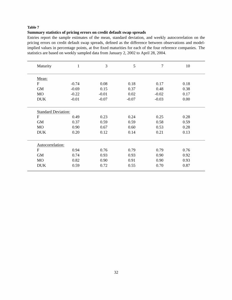
Table 7Summary statistics of pricing errors on credit default swap spreadsEntries report the sample estimates of the mean, standard deviation, and weekly autocorrelation on thepricing errors on credit default swap spreads, defined as the difference between observations and model-implied values in percentage points, at five fixed maturities for each of the four reference companies. Thestatistics are based on weekly sampled data from January 2, 2002 to April 28, 2004.

Maturity 1 3 5 7 10

Mean:F -0.74 0.08 0.18 0.17 0.18GM -0.69 0.15 0.37 0.48 0.38MO -0.22 -0.01 0.02 -0.02 0.17DUK -0.01 -0.07 -0.07 -0.03 0.00

Standard Deviation:F 0.49 0.23 0.24 0.25 0.28GM 0.37 0.59 0.59 0.58 0.59MO 0.90 0.67 0.60 0.53 0.28DUK 0.20 0.12 0.14 0.21 0.13

Autocorrelation:F 0.94 0.76 0.79 0.79 0.76GM 0.74 0.93 0.93 0.90 0.92MO 0.82 0.90 0.91 0.90 0.93DUK 0.59 0.72 0.55 0.70 0.87

32

Table 8Maximum likelihood estimates of model parametersEntries in panel A report the model parameter estimates and absolute values of the t-statistics (in parenthe-ses), estimated for each of the four reference companies. The estimation isbased on weekly sampled datafrom January 2, 2002 to April 30, 2004. Panel B reports the estimates and t-statistics for the market price ofrisk for the two risk factors (zandv), computed from the model parameter estimates and covariance matrix.

Companies F GM MO DUK

Panel A: Joint Dynamics

κv 3.8468 ( 48.59 ) 10.4027 ( 70.58 ) 6.3873 ( 57.59 ) 6.9237 ( 92.13 )κz 0.0069 ( 0.61 ) 0.7467 ( 7.21 ) 0.0000 ( 0.81 ) 0.0226 ( 1.42 )κP

v 1.2314 ( 1.99 ) 2.0402 ( 34.14 ) 1.2440 ( 4.31 ) 2.2879 ( 2.78 )κP

z 0.1704 ( 1.62 ) 1.7434 ( 2.25 ) 0.5690 ( 1.04 ) 0.1109 ( 1.72 )θv 0.2620 ( 22.87 ) 0.7047 ( 52.86 ) 0.2757 ( 39.40 ) 0.5744 ( 79.50 )θz 0.0033 ( 1.74 ) 0.0000 ( 0.00 ) 0.0287 ( 4.75 ) 0.0015 ( 0.53 )σv 1.0622 ( 67.43 ) 0.6412 ( 26.84 ) 0.7912 ( 87.67 ) 1.3258 ( 65.53 )σz 0.1863 ( 21.81 ) 2.8890 ( 46.13 ) 1.5635 ( 57.00 ) 0.3919 ( 28.95 )ξ 0.4328 ( 28.54 ) 0.4477 ( 24.55 ) 0.2506 ( 14.77 ) 0.1580 ( 19.21 )κzv -0.0140 ( 0.51 ) -0.4393 ( 2.50 ) -0.0996 ( 0.74 ) -0.0539 ( 1.69 )ρsv -0.0620 ( 6.57 ) -0.2931 ( 33.52 ) -0.1953 ( 27.35 ) -0.4882 ( 83.29 )

Panel B: Market Prices of Risks

γv 2.4623 ( 4.12 ) 13.0413 ( 33.05 ) 6.5010 ( 15.26 ) 3.4966 ( 5.28 )γz -0.8776 ( 1.60 ) -0.3450 ( 1.34 ) -0.3639 ( 1.04 ) -0.2253 ( 1.44 )

33

20 30 40 50 60 70 8040

42

44

46

48

50

52

Put Option Delta

Impl

ied

Vol

atlit

y, %

F

20 30 40 50 60 70 8030

32

34

36

38

40

42

Put Option Delta

Impl

ied

Vol

atlit

y, %

GM

20 30 40 50 60 70 8026

27

28

29

30

31

32

33

34

Put Option Delta

Impl

ied

Vol

atlit

y, %

MO

20 30 40 50 60 70 8032

34

36

38

40

42

44

46

48

Put Option Delta

Impl

ied

Vol

atlit

y, %

DUK

Figure 1The average implied volatility smirk on stock optionsLines are the average implied volatility plotted against put option delta at three fixed maturities: one month(solid lines), two months (dashed lines), and three months (dash-dotted lines). Each panel is for one com-pany.

34

Dec01 Mar02 Jul02 Oct02 Jan03 Apr03 Aug03 Nov03 Feb04 Jun040

5

10

CD

S S

prea

d, %

F


100

200

AT

M Im

plie

d V

olat

ility

, %


1

2

3

4

5

CD

S S

prea

d, %

GM


20

40

60

80

100

ATM

Impl

ied

Vol

atili

ty, %


2

4

6

8

10

CD

S S

prea

d, %

MO


20

40

60

80

100

AT

M Im

plie

d V

olat

ility

, %


5

10

CD

S S

prea

d, %

DUK


50

100

AT

M Im

plie

d V

olat

ility

, %Figure 2Time series of credit default swap spreads and at-the-money stock option implied volatilities.The solid lines are the time series of credit default swap rates at fixed maturities of one, three, five, seven,and ten years, with scales on the left hand size. The dashed lines are the timeseries of the at-the-money (50delta) stock option implied volatilities at fixed maturities of 30, 60, and 91 days, withthe scales on the righthand side.

35

20 30 40 50 60 70 80 90 1001

2

3

4

5

6

7

8

9

CD

S, %

Implied Volatility, %

R2=82.2393%

F

20 30 40 50 60 70 801

1.5

2

2.5

3

3.5

4

4.5

5

CD

S, %


R2=59.1953%

GM

10 20 30 40 50 60 70 800.5

1

1.5

2

2.5

3

3.5

4

4.5

5

5.5

CD

S, %


R2=36.3958%

MO

20 30 40 50 60 70 800

1

2

3

4

5

6

CD

S, %


R2=67.2625%

DUK

Figure 3Regression credit default swap spreads on stock option implied volatilities.Circles are data points that correspond to the five-year credit default swap spreads on they-axis and thethree-month at-the-money implied volatilities on thex-axis. The solid line denotes the least square fitting.

36

−20 −15 −10 −5 0 5 10 15 20−0.15

−0.1

−0.05

0

0.05

0.1

0.15

0.2

0.25

Number of Lags in Days

Sam

ple

Cro

ss C

orre

latio

n

F: [∆ CDS (Lag), ∆ ATMV]

−20 −15 −10 −5 0 5 10 15 20−0.15

−0.1

−0.05

0

0.05

0.1

0.15

0.2

0.25

0.3

Number of Lags in DaysS

ampl

e C

ross

Cor

rela

tion

GM: [∆ CDS (Lag), ∆ ATMV]

−20 −15 −10 −5 0 5 10 15 20−0.3

−0.2

−0.1

0

0.1

0.2

0.3

0.4

0.5


Sam

ple

Cro

ss C

orre

latio

n

MO: [∆ CDS (Lag), ∆ ATMV]

−20 −15 −10 −5 0 5 10 15 20−0.15

−0.1

−0.05

0

0.05

0.1

0.15

0.2

0.25


Sam

ple

Cro

ss C

orre

latio

n

DUK: [∆ CDS (Lag), ∆ ATMV]

Figure 4Cross-correlogram between daily changes in the five-year credit default swap spread and the three-month at-the-money implied volatility.The bars show the correlation estimates between daily changes in the five-year credit default swap spreadand daily changes in the three-month at-the-money implied volatility at different leads and lags. The twodash-dotted lines in each panel define the 95 percent confidence band.

37

0 2 4 6 8 100

0.5

1

1.5

2

2.5

Maturity, Years

Cred

it Sp

read

Res

pons

e

F

0 2 4 6 8 100

0.1

0.2

0.3

0.4

0.5

0.6

0.7

0.8

0.9

1

Maturity, Years

Cred

it Sp

read

Res

pons

e

GM

0 2 4 6 8 100

0.1

0.2

0.3

0.4

0.5

0.6

0.7

0.8

0.9

1

Maturity, Years

Cred

it Sp

read

Res

pons

e

MO

0 2 4 6 8 100

0.1

0.2

0.3

0.4

0.5

0.6

0.7

0.8

0.9

1

Maturity, Years

Cred

it Sp

read

Res

pons

e

DUK

Figure 5The contemporaneous response of the credit spread to unit shocks in the two risk factorsLines denote the contemporaneous response of the credit spread, defined as the difference between contin-uously compounded spot rate of a reference company and the corresponding spot rate for the libor/swapmarket, to unit shocks to the two sources of risksz (solid lines) andv (dashed lines).

38


0.5

1

v t


0.1

0.2

z t


0.1

0.2

0.3

0.4

0.5

0.6

0.7

v tDec01 Mar02 Jul02 Oct02 Jan03 Apr03 Aug03 Nov03 Feb04 Jun04

0

0.05

0.1

0.15

0.2

0.25

0.3

0.35

z t


0.1

0.2

0.3

0.4

v t


0.05

0.1

0.15

0.2

z t


0.2

0.4

0.6

0.8

v t


0.05

0.1

0.15

0.2

z tFigure 6The time series of return variance rates and default arrival rates.Solid lines are the extracted time series of the instantaneous variance rate on the diffusion component of thestock return, with the scales on the left hand side. Dashed lines are the extracted time series of the defaultarrival rate on the reference companies, with the scales on the right hand side.

39

stock options and credit default swaps: a joint framework for

Documents