Steven R. DunbarDepartment of Mathematics203 Avery HallUniversity of Nebraska-LincolnLincoln, NE 68588-0130http://www.math.unl.edu

Voice: 402-472-3731Fax: 402-472-8466

Stochastic Processes and

Advanced Mathematical Finance

Solution of the Black-Scholes Equation

Rating

Mathematically Mature: may contain mathematics beyond calculus withproofs.

1

Section Starter Question

What is the solution method for the Cauchy-Euler type of ordinary differen-tial equation:

x2d2v

dx2+ ax

dv

dx+ bv = 0 ?

Key Concepts

1. We solve the Black-Scholes equation for the value of a European calloption on a security by judicious changes of variables that reduce theequation to the heat equation. The heat equation has a solution for-mula. Using the solution formula with the changes of variables givesthe solution to the Black-Scholes equation.

2. Solving the Black-Scholes equation is an example of how to choose andexecute changes of variables to solve a partial differential equation.

Vocabulary

1. A differential equation with auxiliary initial conditions and boundaryconditions, that is an initial value problem, is said to be well-posedif the solution exists, is unique, and small changes in the equationparameters, the initial conditions or the boundary conditions produceonly small changes in the solutions.

2

Mathematical Ideas

Conditions for Solution of the Black-Scholes Equation

We have to start somewhere, and to avoid the problem of deriving everythingback to calculus, we will assert that the initial value problem for the heatequation on the real line is well-posed. That is, consider the solution to thepartial differential equation

∂u

∂τ=∂2u

∂x2−∞ < x <∞, τ > 0

with the initial conditionu(x, 0) = u0(x).

Assume the initial condition and the solution satisfy the following technicalrequirements:

1. u0(x) has at most a finite number of discontinuities of the jump kind.

2. lim|x|→∞ u0(x)e−ax2

= 0 for any a > 0.

3. lim|x|→∞ u(x, τ)e−ax2

= 0 for any a > 0.

Under these mild assumptions, the solution exists for all time and is unique.Most importantly, the solution is represented as

u(x, τ) =1

2√πτ

∫ ∞−∞

u0(s)e−(x−s)2

4τ ds .

Remark. This solution can be derived in several different ways, the easiestway is to use Fourier transforms. The derivation of this solution representa-tion is standard in any course or book on partial differential equations.

3

Remark. Mathematically, the conditions above are unnecessarily restrictive,and can be considerably weakened. However, they will be more than sufficientfor all practical situations we encounter in mathematical finance.

Remark. The use of τ for the time variable (instead of the more natural t)is to avoid a conflict of notation in the several changes of variables we willsoon have to make.

The Black-Scholes terminal value problem for the value V (S, t) of a Eu-ropean call option on a security with price S at time t is

∂V

∂t+

1

2σ2S2∂

2V

∂S2+ rS

∂V

∂S− rV = 0

with V (0, t) = 0, V (S, t) ∼ S as S →∞ and

V (S, T ) = max(S −K, 0).

Note that this looks a little like the heat equation on the infinite intervalin that it has a first derivative of the unknown with respect to time and thesecond derivative of the unknown with respect to the other (space) variable.On the other hand, notice:

1. Each time the unknown is differentiated with respect to S, it also mul-tiplied by the independent variable S, so the equation is not a constantcoefficient equation.

2. There is a first derivative of V with respect to S in the equation.

3. There is a zero-th order derivative term V in the equation.

4. The sign on the second derivative is the opposite of the heat equationform, so the equation is of backward parabolic form.

5. The data of the problem is given at the final time T instead of the initialtime 0, consistent with the backward parabolic form of the equation.

6. There is a boundary condition V (0, t) = 0 specifying the value of thesolution at one sensible boundary of the problem. The boundary is sen-sible since security values must only be zero or positive. This boundarycondition says that any time the security value is 0, then the call value(with strike price K) is also worth 0.

4

7. There is another boundary condition V (S, t) ∼ S, as S → ∞, butalthough this is financially sensible, (it says that for very large securityprices, the call value with strike price K is approximately S) it is morein the nature of a technical condition, and we will ignore it withoutconsequence.

We eliminate each objection with a suitable change of variables. The planis to change variables to reduce the Black-Scholes terminal value problem tothe heat equation, then to use the known solution of the heat equation torepresent the solution, and finally change variables back. This is a standardsolution technique in partial differential equations. All the transformationsare standard and well-motivated.

Solution of the Black-Scholes Equation

First we take t = T − τ(1/2)σ2 and S = Kex, and we set

V (S, t) = Kv(x, τ).

Remember, σ is the volatility, r is the interest rate on a risk-free bond, andK is the strike price. In the changes of variables above, the choice for treverses the sense of time, changing the problem from backward parabolicto forward parabolic. The choice for S is a well-known transformation basedon experience with the Euler equidimensional equation in differential equa-tions. In addition, the variables have been carefully scaled so as to makethe transformed equation expressed in dimensionless quantities. All of thesetechniques are standard and are covered in most courses and books on partialdifferential equations and applied mathematics.

Some extremely wise advice adapted from Stochastic Calculus and Fi-nancial Applications by J. Michael Steele, [1, page 186], is appropriate here.

“There is nothing particularly difficult about changing vari-ables and transforming one equation to another, but there is anelement of tedium and complexity that slows us down. There isno universal remedy for this molasses effect, but the calculationsdo seem to go more quickly if one follows a well-defined plan. Ifwe know that V (S, t) satisfies an equation (like the Black-Scholesequation) we are guaranteed that we can make good use of theequation in the derivation of the equation for a new function

5

v(x, τ) defined in terms of the old if we write the old V as a func-tion of the new v and write the new τ and x as functions of theold t and S. This order of things puts everything in the directline of fire of the chain rule; the partial derivatives Vt, VS and VSSare easy to compute and at the end, the original equation standsready for immediate use.”

Following the advice, write

τ =σ2

2· (T − t)

and

x = log

(S

K

).

The first derivatives are

∂V

∂t= K

∂v

∂τ· dτdt

= K∂v

∂τ· −σ

2

2

and∂V

∂S= K

∂v

∂x· dxdS

= K∂v

∂x· 1

S.

The second derivative is

∂2V

∂S2=

∂

∂S

(∂V

∂S

)=

∂

∂S

(K∂v

∂x

1

S

)= K

∂v

∂x· −1

S2+K

∂

∂S

(∂v

∂x

)· 1

S

= K∂v

∂x· −1

S2+K

∂

∂x

(∂v

∂x

)· dxdS· 1

S

= K∂v

∂x· −1

S2+K

∂2v

∂x2· 1

S2.

The terminal condition is

V (S, T ) = max(S −K, 0) = max(Kex −K, 0)

but V (S, T ) = Kv(x, 0) so v(x, 0) = max(ex − 1, 0).

6

Now substitute all of the derivatives into the Black-Scholes equation toobtain:

K∂v

∂τ· −σ

2

2+σ2

2S2

(K∂v

∂x· −1

S2+K

∂2v

∂x2· 1

S2

)+ rS

(K∂v

∂x· 1

S

)− rKv = 0.

Now begin the simplification:

1. Divide out the common factor K.

2. Transpose the τ -derivative to the other side, and divide through by σ2

2.

3. Rename the remaining constant rσ2/2

as k which measures the ratiobetween the risk-free interest rate and the volatility.

4. Cancel the S2 terms in the second derivative.

5. Cancel the S terms in the first derivative.

6. Gather up like order terms.

What remains is the rescaled, constant coefficient equation:

∂v

∂τ=∂2v

∂x2+ (k − 1)

∂v

∂x− kv.

1. Now there is only one dimensionless parameter k measuring the risk-free interest rate as a multiple of the volatility and a rescaled time toexpiry σ2

2T , not the original 4 dimensioned quantities K, T , σ2 and r.

2. The equation is defined on the interval −∞ < x < ∞, since this x-interval defines 0 < S <∞ through the change of variables S = Kex.

3. The equation now has constant coefficients.

In principle, we could now solve the equation directly.Instead, we will simplify further by changing the dependent variable scale

yet again, byv = eαx+βτu(x, τ)

where α and β are yet to be determined. Using the product rule:

vτ = βeαx+βτu+ eαx+βτuτ

7

andvx = αeαx+βτu+ eαx+βτux

andvxx = α2eαx+βτu+ 2αeαx+βτux + eαx+βτuxx.

Put these into our constant coefficient partial differential equation, dividethe common factor of eαx+βτ throughout and obtain:

βu+ uτ = α2u+ 2αux + uxx + (k − 1)(αu+ ux)− ku.

Gather like terms:

uτ = uxx + [2α + (k − 1)]ux + [α2 + (k − 1)α− k − β]u.

Choose α = −k−12

so that the ux coefficient is 0, and then choose β =

α2 + (k − 1)α − k = − (k+1)2

4so the u coefficient is likewise 0. With this

choice, the equation is reduced to

uτ = uxx.

We need to transform the initial condition too. This transformation is

u(x, 0) = e−(−(k−1)

2)x−(− (k+1)2

4)·0v(x, 0)

= e((k−1)

2)x max(ex − 1, 0)

= max(e(

(k+1)2 )x − e(

(k−1)2 )x, 0

).

For future reference, we notice that this function is strictly positive whenthe argument x is strictly positive, that is u0(x) > 0 when x > 0, otherwise,u0(x) = 0 for x ≤ 0.

We are in the final stage since we are ready to apply the heat-equationsolution representation formula:

u(x, τ) =1

2√πτ

∫ ∞−∞

u0(s)e− (x−s)2

4τ ds .

However, first we want to make a change of variable in the integration, bytaking z = (s−x)√

2τ, (and thereby dz = (− 1√

2τ) dx) so that the integration

becomes:

u(x, τ) =1√2π

∫ ∞−∞

u0

(z√

2τ + x)e−

z2

2 dz .

8

We may as well only integrate over the domain where u0 > 0, that is for

z > − x√2τ

. On that domain, u0 = ek+12 (x+z

√2τ) − e

k−12 (x+z

√2τ) so we are

down to:

1√2π

∫ ∞−x/√2τ

ek+12 (x+z

√2τ)e−

z2

2 dz− 1√2π

∫ ∞−x/√2τ

ek−12 (x+z

√2τ)e−

z2

2 dz .

Call the two integrals I1 and I2 respectively.We will evaluate I1 (the integral with the k + 1 term) first. This is easy,

completing the square in the exponent yields a standard, tabulated integral.The exponent is

k + 1

2

(x+ z

√2τ)− z2

2

=

(−1

2

)(z2 −

√2τ (k + 1) z

)+

(k + 1

2

)x

=

(−1

2

)(z2 −

√2τ (k + 1) z + τ

(k + 1)2

2

)+

((k + 1)

2

)x+ τ

(k + 1)2

4

=

(−1

2

)(z −

√τ/2 (k + 1)

)2+

(k + 1)x

2+τ (k + 1)2

4.

Therefore

1√2π

∫ ∞−x/√2τ

ek+12 (x+z

√2τ)e−

z2

2 dz

=e

(k+1)x2

+τ(k+1)2

4

√2π

∫ ∞−x/√2τ

e− 1

2

(z−√τ/2(k+1)

)2

dz .

Now, change variables again on the integral, choosing y = z −√τ/2 (k + 1)

so dy = dz, and all we need to change are the limits of integration:

e(k+1)x

2+τ

(k+1)2

4

√2π

∫ ∞−x/√2τ−√τ/2(k+1)

e

(− y

2

2

)dz .

The integral can be represented in terms of the cumulative distribution func-tion of a normal random variable, usually denoted Φ. That is,

Φ(d) =1√2π

∫ d

−∞e−

y2

2 dy

9

so

I1 = e(k+1)x

2+τ

(k+1)2

4 Φ(d1)

where d1 = x√2τ

+√

τ2

(k + 1). Note the use of the symmetry of the integral!

The calculation of I2 is identical, except that (k + 1) is replaced by (k − 1)throughout.

The solution of the transformed heat equation initial value problem is

u(x, τ) = e(k+1)x

2+τ(k+1)2

4 Φ(d1)− e(k−1)x

2+τ(k−1)2

4 Φ(d2)

where d1 = x√2τ

+√

τ2

(k + 1) and d2 = x√2τ

+√

τ2

(k − 1).Now we must systematically unwind each of the changes of variables,

starting from u. First, v(x, τ) = e−(k−1)x

2− (k+1)2τ

4 u(x, τ). Notice how manyof the exponentials neatly combine and cancel! Next put x = log (S/K),τ =

(12

)σ2(T − t) and V (S, t) = Kv(x, τ).

The ultimate result is the Black-Scholes formula for the value of a Eu-ropean call option at time T with strike price K, if the current time is tand the underlying security price is S, the risk-free interest rate is r and thevolatility is σ:

V (S, t) = SΦ

(log(S/K) + (r + σ2/2)(T − t)

σ√T − t

)−Ke−r(T−t)Φ

(log(S/K) + (r − σ2/2)(T − t)

σ√T − t

).

Usually one doesn’t see the solution as this full closed form solution. Mostversions of the solution write intermediate steps in small pieces, and thenpresent the solution as an algorithm putting the pieces together to obtainthe final answer. Specifically, let

d1 =log(S/K) + (r + σ2/2)(T − t)

σ√T − t

d2 =log(S/K) + (r − σ2/2)(T − t)

σ√T − t

and writing VC(S, t) to remind ourselves this is the value of a call option,

VC(S, t) = S · Φ (d1)−Ke−r(T−t) · Φ (d2) .

10

0

10

20

30

Option

Value

70 90 110 130Share Price

Figure 1: Value of the call option at maturity.

Solution of the Black-Scholes Equation Graphically

Consider for purposes of graphical illustration the value of a call option withstrike price K = 100. The risk-free interest rate per year, continuouslycompounded is 12%, so r = 0.12, the time to expiration is T = 1 measuredin years, and the standard deviation per year on the return of the stock, orthe volatility is σ = 0.10. The value of the call option at maturity plottedover a range of stock prices 70 ≤ S ≤ 130 surrounding the strike price isillustrated in 1

We use the Black-Scholes formula above to compute the value of theoption before expiration. With the same parameters as above the value ofthe call option is plotted over a range of stock prices 70 ≤ S ≤ 130 at timeremaining to expiration t = 1 (red), t = 0.8, (orange), t = 0.6 (yellow),t = 0.4 (green), t = 0.2 (blue) and at expiration t = 0 (black).

Using this graph, notice two trends in the option value:

1. For a fixed time, as the stock price increases the option value increases.

2. As the time to expiration decreases, for a fixed stock value the value ofthe option decreases to the value at expiration.

We predicted both trends from our intuitive analysis of options, see Options.The Black-Scholes option pricing formula makes the intuition precise.

We can also plot the solution of the Black-Scholes equation as a functionof security price and the time to expiration as value surface.

This value surface shows both trends.

11

0

10

20

30

40

Option

Value

70 90 110 130Share Price

Figure 2: Value of the call option at various times.

Figure 3: Value surface from the Black-Scholes formula.

12

Sources

This discussion is drawn from Section 4.2, pages 59–63; Section 4.3, pages66–69; Section 5.3, pages 75–76; and Section 5.4, pages 77–81 of The Math-ematics of Financial Derivatives: A Student Introduction by P. Wilmott, S.Howison, J. Dewynne, Cambridge University Press, Cambridge, 1995. Someideas are also taken from Chapter 11 of Stochastic Calculus and FinancialApplications by J. Michael Steele, Springer, New York, 2001.

Algorithms, Scripts, Simulations

Algorithm

For given parameter values, the Black-Scholes-Merton solution formula issampled at a specified m × 1 array of times and at a specified 1 × n arrayof security prices using vectorization and broadcasting. The result can beplotted as functions of the security price as done in the text. The calculationis vectorized for an array of S values and an array of t values, but it isnot vectorized for arrays in the parameters K, r, T , and σ. This approachis taken to illustrate the use of vectorization and broadcasting for efficientevaluation of an array of solution values from a complicated formula.

In particular, the calculation of d1 and d2 then uses broadcasting, alsocalled binary singleton expansion, recycling, single-instruction multiple data,threading or replication.

The calculation relies on using the rules for calcuation and handling ofinfinity and NaN (Not a Number) which come from divisions by 0, takinglogarithms of 0, and negative numbers and calculating the normal cdf atinfinity and negative infinity. The plotting routines will not plot a NaNwhich accounts for the gap at S = 0 in the graph line for t = 1.

Scripts

Geogebra GeoGebra applet for graphing the Black-Scholes solution

13

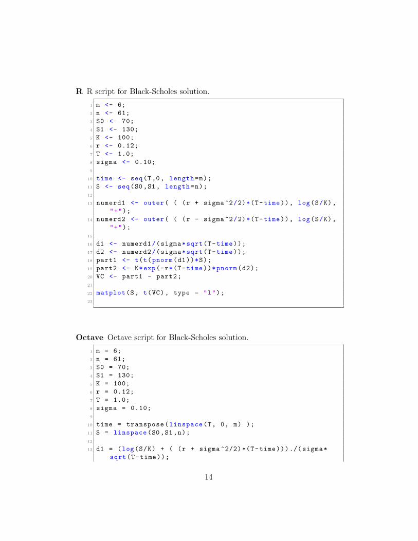
R R script for Black-Scholes solution.

1 m <- 6;

2 n <- 61;

3 S0 <- 70;

4 S1 <- 130;

5 K <- 100;

6 r <- 0.12;

7 T <- 1.0;

8 sigma <- 0.10;

9

10 time <- seq(T,0, length=m);

11 S <- seq(S0,S1, length=n);

12

13 numerd1 <- outer( ( (r + sigma^2/2)*(T-time)), log(S/K),

"+");

14 numerd2 <- outer( ( (r - sigma^2/2)*(T-time)), log(S/K),

"+");

15

16 d1 <- numerd1/(sigma*sqrt(T-time));

17 d2 <- numerd2/(sigma*sqrt(T-time));

18 part1 <- t(t(pnorm(d1))*S);

19 part2 <- K*exp(-r*(T-time))*pnorm(d2);

20 VC <- part1 - part2;

21

22 matplot(S, t(VC), type = "l");

23

Octave Octave script for Black-Scholes solution.

1 m = 6;

2 n = 61;

3 S0 = 70;

4 S1 = 130;

5 K = 100;

6 r = 0.12;

7 T = 1.0;

8 sigma = 0.10;

9

10 time = transpose(linspace(T, 0, m) );

11 S = linspace(S0,S1,n);

12

13 d1 = (log(S/K) + ( (r + sigma ^2/2)*(T-time)))./( sigma*

sqrt(T-time));

14

14 d2 = (log(S/K) + ( (r - sigma ^2/2)*(T-time)))./( sigma*

sqrt(T-time));

15 part1 = bsxfun(@times , normcdf(d1), S);

16 part2 = bsxfun( @times , K*exp(-r*(T-time)), normcdf(d2));

17 VC = part1 - part2;

18

19 plot(S,VC)

20

Perl Perl PDL script for Black-Scholes solution.

1 sub pnorm {

2 my ( $x , $sigma , $mu ) = @_;

3 $sigma = 1 unless defined($sigma);

4 $mu = 0 unless defined($mu);

5

6 return 0.5 * ( 1 + erf( ( $x - $mu ) / ( sqrt (2) *

$sigma ) ) );

7 }

8 $m = 6;

9 $n = 61;

10 $S0 = 70;

11 $S1 = 130;

12 $K = 100;

13 $r = 0.12;

14 $T = 1.0;

15 $sigma = 0.10;

16

17 $time = zeroes($m)->xlinvals($T ,0.0);

18 $S = zeroes($n)->xlinvals($S0 ,$S1);

19

20 $logSoverK = log($S/$K);

21 $n12 = (($r + $sigma **2/2) *($T -$time));

22 $n22 = (($r - $sigma **2/2) *($T -$time));

23 $numerd1 = $logSoverK + $n12 ->transpose;

24 $numerd2 = $logSoverK + $n22 ->transpose;

25 $d1 = $numerd1 /( ($sigma*sqrt($T -$time))->transpose);

26 $d2 = $numerd2 /( ($sigma*sqrt($T -$time))->transpose);

27

28 $part1 = $S * pnorm($d1);

29 $part2 = pnorm($d2) * ($K*exp(-$r*($T -$time)))->transpose

;

30 $VC = $part1 - $part2;

31

15

32 # file output to use with external plotting programming

33 # such as gnuplot , R, octave , etc.

34 # Start gnuplot , then from gnuplot prompt

35 # plot for [n=2:7] ’solution.dat’ using 1:( column(n))

with lines

36

37

38 open( F, ">solution.dat" ) || die "cannot write: $! ";

39 wcols $S, $VC , *F;

40 close(F);

41

SciPy Scientific Python script for Black-Scholes solution.

1 import scipy

2

3 m = 6

4 n = 61

5 S0 = 70

6 S1 = 130

7 K = 100

8 r = 0.12

9 T = 1.0

10 sigma = 0.10

11

12 time = scipy.linspace(T, 0.0, m)

13 S = scipy.linspace(S0,S1, n)

14

15 logSoverK = scipy.log(S/K)

16 n12 = ((r + sigma **2/2) *(T-time))

17 n22 = ((r - sigma **2/2) *(T-time))

18 numerd1 = logSoverK[scipy.newaxis ,:] + n12[:,scipy.

newaxis]

19 numerd2 = logSoverK[scipy.newaxis ,:] + n22[:,scipy.

newaxis]

20 d1 = numerd1 /(sigma*scipy.sqrt(T-time)[:,scipy.newaxis ])

21 d2 = numerd2 /(sigma*scipy.sqrt(T-time)[:,scipy.newaxis ])

22

23 from scipy.stats import norm

24 part1 = S[scipy.newaxis] * norm.cdf(d1)

25 part2 = norm.cdf(d2) * K*scipy.exp(-r*(T-time))[:,scipy.

newaxis]

26 VC = part1 - part2

27

16

28 # optional file output to use with external plotting

programming

29 # such as gnuplot , R, octave , etc.

30 # Start gnuplot , then from gnuplot prompt

31 # plot for [n=2:7] ’solution.dat’ using 1:( column(n))

with lines

32

33 scipy.savetxt(’solution.dat’,

34 scipy.column_stack ((scipy.transpose(S),scipy.

transpose(VC))),

35 fmt=(’%4.3f’))

Problems to Work for Understanding

1. Explicitly evaluate the integral I2 in terms of the c.d.f. Φ and otherelementary functions as was done for the integral I1.

2. What is the price of a European call option on a non-dividend-payingstock when the stock price is $52, the strike price is $50, the risk-free interest rate is 12% per annum (compounded continuously), thevolatility is 30% per annum, and the time to maturity is 3 months?

3. What is the price of a European call option on a non-dividend payingstock when the stock price is $30, the exercise price is $29, the risk-freeinterest rate is 5%, the volatility is 25% per annum, and the time tomaturity is 4 months?

4. Show that the Black-Scholes formula for the price of a call option tendsto max(S −K, 0) as t→ T .

5. For a particular scripting language of your choice, modify the scriptsto create a function within that language that will evaluate the Black-Scholes formula for a call option at a time and security value for givenparameters.

17

6. For a particular scripting language of your choice, modify the scripts tocreate a script within that language that will evaluate the Black-Scholesformula for a call option at a specified time for given parameters, andreturn a function of the security prices that can plotted by calling thefunction over an interval of security prices.

7. Plot the price of a European call option on a non-dividend paying stockover the stock prices $20 to $40, given that the exercise price is $29,the risk-free interest rate is 5%, the volatility is 25% per annum, andthe time to maturity is 4 months.

8. For a particular scripting language of your choice, modify the scriptsto create a script within that language that will plot the Black-Scholessolution for VC(S, t) as a surface over the two variables S and t.

Reading Suggestion:

References

[1] J. Michael Steele. Stochastic Calculus and Financial Applications.Springer-Verlag, 2001. QA 274.2 S 74.

[2] Paul Wilmott, S. Howison, and J. Dewynne. The Mathematics of Finan-cial Derivatives. Cambridge University Press, 1995.

18

Outside Readings and Links:

1. Cornell University, Department of Computer Science, Prof. T. Cole-man Rhodes and Prof. R. Jarrow Numerical Solution of Black-ScholesEquation, Submitted by Chun Fan, Nov. 12, 2002.

2. An applet for calculating the option value based on the Black-Scholesmodel. Also contains tips on options, business news and literature onoptions. Submitted by Yogesh Makkar, November 19, 2003.

I check all the information on each page for correctness and typographicalerrors. Nevertheless, some errors may occur and I would be grateful if you wouldalert me to such errors. I make every reasonable effort to present current andaccurate information for public use, however I do not guarantee the accuracy ortimeliness of information on this website. Your use of the information from thiswebsite is strictly voluntary and at your risk.

I have checked the links to external sites for usefulness. Links to externalwebsites are provided as a convenience. I do not endorse, control, monitor, orguarantee the information contained in any external website. I don’t guaranteethat the links are active at all times. Use the links here with the same caution asyou would all information on the Internet. This website reflects the thoughts, in-terests and opinions of its author. They do not explicitly represent official positionsor policies of my employer.

Information on this website is subject to change without notice.

Steve Dunbar’s Home Page, http://www.math.unl.edu/~sdunbar1Email to Steve Dunbar, sdunbar1 at unl dot edu

Last modified: Processed from LATEX source on August 10, 2016

19