mathematical modeling in finance with stochastic...
TRANSCRIPT

Mathematical Modeling in Finance withStochastic Processes
Steven R. Dunbar
February 5, 2011

2

Contents
1 Background Ideas 7
1.1 Brief History of Mathematical Finance . . . . . . . . . . . . . 7
1.2 Options and Derivatives . . . . . . . . . . . . . . . . . . . . . 17
1.3 Speculation and Hedging . . . . . . . . . . . . . . . . . . . . . 25
1.4 Arbitrage . . . . . . . . . . . . . . . . . . . . . . . . . . . . . 32
1.5 Mathematical Modeling . . . . . . . . . . . . . . . . . . . . . 38
1.6 Randomness . . . . . . . . . . . . . . . . . . . . . . . . . . . . 48
1.7 Stochastic Processes . . . . . . . . . . . . . . . . . . . . . . . 55
1.8 A Binomial Model of Mortgage Collateralized Debt Obliga-tions (CDOs) . . . . . . . . . . . . . . . . . . . . . . . . . . . 64
2 Binomial Option Pricing Models 73
2.1 Single Period Binomial Models . . . . . . . . . . . . . . . . . . 73
2.2 Multiperiod Binomial Tree Models . . . . . . . . . . . . . . . 81
3 First Step Analysis for Stochastic Processes 89
3.1 A Coin Tossing Experiment . . . . . . . . . . . . . . . . . . . 89
3.2 Ruin Probabilities . . . . . . . . . . . . . . . . . . . . . . . . . 94
3.3 Duration of the Gambler’s Ruin . . . . . . . . . . . . . . . . 106
3.4 A Stochastic Process Model of Cash Management . . . . . . . 113
4 Limit Theorems for Stochastic Processes 123
4.1 Laws of Large Numbers . . . . . . . . . . . . . . . . . . . . . 123
4.2 Moment Generating Functions . . . . . . . . . . . . . . . . . . 128
4.3 The Central Limit Theorem . . . . . . . . . . . . . . . . . . . 134
4.4 The Absolute Excess of Heads over Tails . . . . . . . . . . . . 145
3
4 CONTENTS
5 Brownian Motion 1555.1 Intuitive Introduction to Diffusions . . . . . . . . . . . . . . . 1555.2 The Definition of Brownian Motion and the Wiener Process . 1615.3 Approximation of Brownian Motion by Coin-Flipping Sums . . 1715.4 Transformations of the Wiener Process . . . . . . . . . . . . . 1745.5 Hitting Times and Ruin Probabilities . . . . . . . . . . . . . . 1795.6 Path Properties of Brownian Motion . . . . . . . . . . . . . . 1835.7 Quadratic Variation of the Wiener Process . . . . . . . . . . . 186
6 Stochastic Calculus 1956.1 Stochastic Differential Equations and the Euler-Maruyama Method1956.2 Ito’s Formula . . . . . . . . . . . . . . . . . . . . . . . . . . . 2016.3 Properties of Geometric Brownian Motion . . . . . . . . . . . 207
7 The Black-Scholes Model 2157.1 Derivation of the Black-Scholes Equation . . . . . . . . . . . . 2157.2 Solution of the Black-Scholes Equation . . . . . . . . . . . . . 2237.3 Put-Call Parity . . . . . . . . . . . . . . . . . . . . . . . . . . 2367.4 Derivation of the Black-Scholes Equation . . . . . . . . . . . . 2447.5 Implied Volatility . . . . . . . . . . . . . . . . . . . . . . . . . 2527.6 Sensitivity, Hedging and the “Greeks” . . . . . . . . . . . . . . 2567.7 Limitations of the Black-Scholes Model . . . . . . . . . . . . . 264
List of Figures
1.1 This is not the market for options! . . . . . . . . . . . . . . . 20
1.2 Intrinsic value of a call option . . . . . . . . . . . . . . . . . . 22
1.3 A diagram of the cash flow in the gold arbitrage . . . . . . . . 35
1.4 The cycle of modeling . . . . . . . . . . . . . . . . . . . . . . 40
1.5 Initial conditions for a coin flip, from Keller . . . . . . . . . . 52
1.6 Persi Diaconis’ mechanical coin flipper . . . . . . . . . . . . . 53
1.7 The family tree of some stochastic processes . . . . . . . . . . 62
1.8 Default probabilities as a function of both the tranche number0 to 100 and the base mortgage default probability 0.01 to 0.15 70
2.1 The single period binomial model. . . . . . . . . . . . . . . . . 76
2.2 A binomial tree . . . . . . . . . . . . . . . . . . . . . . . . . . 82
2.3 Pricing a European call . . . . . . . . . . . . . . . . . . . . . . 84
2.4 Pricing a European put . . . . . . . . . . . . . . . . . . . . . . 85
3.1 Welcome to my casino! . . . . . . . . . . . . . . . . . . . . . . 91
3.2 Welcome to my casino! . . . . . . . . . . . . . . . . . . . . . . 92
3.3 Several typical cycles in a model of the reserve requirement. . 117
4.1 Block diagram of transform methods. . . . . . . . . . . . . . . 130
4.2 Approximation of the binomial distribution with the normaldistribution. . . . . . . . . . . . . . . . . . . . . . . . . . . . . 140
4.3 The half-integer correction . . . . . . . . . . . . . . . . . . . . 148
4.4 Probability of s excess heads in 500 tosses . . . . . . . . . . . 151
5.1 Graph of the Dow-Jones Industrial Average from August, 2008to August 2009 (blue line) and a random walk with normalincrements with the same mean and variance (brown line). . . 165
5

6 LIST OF FIGURES
5.2 A standardized density histogram of daily close-to-close re-turns on the Pepsi Bottling Group, symbol NYSE:PBG, fromSeptember 16, 2003 to September 15, 2003, up to September13, 2006 to September 12, 2006 . . . . . . . . . . . . . . . . . 165
6.1 The p.d.f. for a lognormal random variable . . . . . . . . . . . 209
7.1 Value of the call option at maturity . . . . . . . . . . . . . . . 2327.2 Value of the call option at various times . . . . . . . . . . . . 2337.3 Value surface from the Black-Scholes formula . . . . . . . . . . 2347.4 Value of the put option at maturity . . . . . . . . . . . . . . . 2417.5 Value of the put option at various times . . . . . . . . . . . . 2427.6 Value surface from the put-call parity formula . . . . . . . . . 2437.7 Value of the call option at various times . . . . . . . . . . . . 2587.8 The red distribution has more probability near the mean, and
a fatter tail (not visible) . . . . . . . . . . . . . . . . . . . . . 268

Chapter 1
Background Ideas
1.1 Brief History of Mathematical Finance
Rating
Everyone.
Section Starter Question
Name as many financial instruments as you can, and name or describe themarket where you would buy them. Also describe the instrument as highrisk or low risk.
Key Concepts
1. Finance theory is the study of economic agents’ behavior allocatingtheir resources across alternative financial instruments and in time inan uncertain environment. Mathematics provides tools to model andanalyze that behavior in allocation and time, taking into account un-certainty.
2. Louis Bachelier’s 1900 math dissertation on the theory of speculationin the Paris markets marks the twin births of both the continuous timemathematics of stochastic processes and the continuous time economicsof option pricing.
7
8 CHAPTER 1. BACKGROUND IDEAS
3. The most important development in terms of impact on practice wasthe Black-Scholes model for option pricing published in 1973.
4. Since 1973 the growth in sophistication about mathematical modelsand their adoption mirrored the extraordinary growth in financial in-novation. Major developments in computing power made the numericalsolution of complex models possible. The increases in computer powersize made possible the formation of many new financial markets andsubstantial expansions in the size of existing ones.
Vocabulary
1. Finance theory is the study of economic agents’ behavior allocatingtheir resources across alternative financial instruments and in time inan uncertain environment.
2. A derivative is a financial agreement between two parties that dependson something that occurs in the future, such as the price or performanceof an underlying asset. The underlying asset could be a stock, a bond, acurrency, or a commodity. Derivatives have become one of the financialworld’s most important risk-management tools. Derivatives can beused for hedging, or for speculation.
3. Types of derivatives: Derivatives come in many types. There arefutures, agreements to trade something at a set price at a given date;options, the right but not the obligation to buy or sell at a givenprice; forwards, like futures but traded directly between two partiesinstead of on exchanges; and swaps, exchanging one lot of obligationsfor another. Derivatives can be based on pretty much anything as longas two parties are willing to trade risks and can agree on a price [48].
Mathematical Ideas
Introduction
One sometime hears that “compound interest is the eighth wonder of theworld”, or the “stock market is just a big casino”. These are colorful say-ings, maybe based in happy or bitter experience, but each focuses on onlyone aspect of one financial instrument. The “time value of money” and
1.1. BRIEF HISTORY OF MATHEMATICAL FINANCE 9
uncertainty are the central elements that influence the value of financial in-struments. When only the time aspect of finance is considered, the toolsof calculus and differential equations are adequate. When only the uncer-tainty is considered, the tools of probability theory illuminate the possibleoutcomes. When time and uncertainty are considered together we begin thestudy of advanced mathematical finance.
Finance is the study of economic agents’ behavior in allocating financialresources and risks across alternative financial instruments and in time inan uncertain environment. Familiar examples of financial instruments arebank accounts, loans, stocks, government bonds and corporate bonds. Manyless familiar examples abound. Economic agents are units who buy and sellfinancial resources in a market, from individuals to banks, businesses, mutualfunds and hedge funds. Each agent has many choices of where to buy, sell,invest and consume assets, each with advantages and disadvantages. Eachagent must distribute their resources among the many possible investmentswith a goal in mind.
Advanced mathematical finance is often characterized as the study of themore sophisticated financial instruments called derivatives. A derivative isa financial agreement between two parties that depends on something thatoccurs in the future, such as the price or performance of an underlying asset.The underlying asset could be a stock, a bond, a currency, or a commod-ity. Derivatives have become one of the financial world’s most importantrisk-management tools. Finance is about shifting and distributing risk andderivatives are especially efficient for that purpose [38]. Two such instru-ments are futures and options. Futures trading, a key practice in modernfinance, probably originated in seventeenth century Japan, but the idea canbe traced as far back as ancient Greece. Options were a feature of the “tulipmania” in seventeenth century Holland. Both futures and options are called“derivatives”. (For the mathematical reader, these are called derivatives notbecause they involve a rate of change, but because their value is derived fromsome underlying asset.) Modern derivatives differ from their predecessors inthat they are usually specifically designed to objectify and price financialrisk.
Derivatives come in many types. There are futures, agreements totrade something at a set price at a given dates; options, the right but not theobligation to buy or sell at a given price; forwards, like futures but tradeddirectly between two parties instead of on exchanges; and swaps, exchangingflows of income from different investments to manage different risk exposure.
10 CHAPTER 1. BACKGROUND IDEAS
For example, one party in a deal may want the potential of rising incomefrom a loan with a floating interest rate, while the other might prefer thepredictable payments ensured by a fixed interest rate. This elementary swapis known as a “plain vanilla swap”. More complex swaps mix the performanceof multiple income streams with varieties of risk [38]. Another more complexswap is a credit-default swap in which a seller receives a regular fee fromthe buyer in exchange for agreeing to cover losses arising from defaults on theunderlying loans. These swaps are somewhat like insurance [38]. These morecomplex swaps are the source of controversy since many people believe thatthey are responsible for the collapse or near-collapse of several large financialfirms in late 2008. Derivatives can be based on pretty much anything as longas two parties are willing to trade risks and can agree on a price. Businessesuse derivatives to shift risks to other firms, chiefly banks. About 95% of theworld’s 500 biggest companies use derivatives. Derivatives with standardizedterms are traded in markets called exchanges. Derivatives tailored for specificpurposes or risks are bought and sold “over the counter” from big banks. The“over the counter” market dwarfs the exchange trading. In November 2009,the Bank for International Settlements put the face value of over the counterderivatives at $604.6 trillion. Using face value is misleading, after off-settingclaims are stripped out the residual value is $3.7 trillion, still a large figure[48].
Mathematical models in modern finance contain deep and beautiful ap-plications of differential equations and probability theory. In spite of theircomplexity, mathematical models of modern financial instruments have hada direct and significant influence on finance practice.
Early History
The origins of much of the mathematics in financial models traces to LouisBachelier’s 1900 dissertation on the theory of speculation in the Paris mar-kets. Completed at the Sorbonne in 1900, this work marks the twin birthsof both the continuous time mathematics of stochastic processes and thecontinuous time economics of option pricing. While analyzing option pric-ing, Bachelier provided two different derivations of the partial differentialequation for the probability density for the Wiener process or Brown-ian motion. In one of the derivations, he works out what is now calledthe Chapman-Kolmogorov convolution probability integral. Along the way,Bachelier derived the method of reflection to solve for the probability func-

1.1. BRIEF HISTORY OF MATHEMATICAL FINANCE 11
tion of a diffusion process with an absorbing barrier. Not a bad performancefor a thesis on which the first reader, Henri Poincare, gave less than a topmark! After Bachelier, option pricing theory laid dormant in the economicsliterature for over half a century until economists and mathematicians re-newed study of it in the late 1960s. Jarrow and Protter [24] speculate thatthis may have been because the Paris mathematical elite scorned economicsas an application of mathematics.
Bachelier’s work was 5 years before Albert Einstein’s 1905 discovery ofthe same equations for his famous mathematical theory of Brownian motion.The editor of Annalen der Physik received Einstein’s paper on Brownian mo-tion on May 11, 1905. The paper appeared later that year. Einstein proposeda model for the motion of small particles with diameters on the order of 0.001mm suspended in a liquid. He predicted that the particles would undergomicroscopically observable and statistically predictable motion. The Englishbotanist Robert Brown had already reported such motion in 1827 while ob-serving pollen grains in water with a microscope. The physical motion is nowcalled Brownian motion in honor of Brown’s description.
Einstein calculated a diffusion constant to govern the rate of motion ofsuspended particles. The paper was Einstein’s attempt to convince physicistsof the molecular and atomic nature of matter. Surprisingly, even in 1905 thescientific community did not completely accept the atomic theory of matter.In 1908, the experimental physicist Jean-Baptiste Perrin conducted a seriesof experiments that empirically verified Einstein’s theory. Perrin therebydetermined the physical constant known as Avogadro’s number for which hewon the Nobel prize in 1926. Nevertheless, Einstein’s theory was very difficultto rigorously justify mathematically. In a series of papers from 1918 to 1923,the mathematician Norbert Wiener constructed a mathematical model ofBrownian motion. Wiener and others proved many surprising facts abouthis mathematical model of Brownian motion, research that continues today.In recognition of his work, his mathematical construction is often called theWiener process. [24]
Growth of Mathematical Finance
Modern mathematical finance theory begins in the 1960s. In 1965 the economistPaul Samuelson published two papers that argue that stock prices fluctuaterandomly [24]. One explained the Samuelson and Fama efficient marketshypothesis that in a well-functioning and informed capital market, asset-

12 CHAPTER 1. BACKGROUND IDEAS
price dynamics are described by a model in which the best estimate of anasset’s future price is the current price (possibly adjusted for a fair expectedrate of return.) Under this hypothesis, attempts to use past price data orpublicly available forecasts about economic fundamentals to predict securityprices are doomed to failure. In the other paper with mathematician HenryMcKean, Samuelson shows that a good model for stock price movements isgeometric Brownian motion. Samuelson noted that Bachelier’s model failedto ensure that stock prices would always be positive, whereas geometric Brow-nian motion avoids this error [24].
The most important development in terms of practice was the 1973 Black-Scholes model for option pricing. The two economists Fischer Black and My-ron Scholes (and simultaneously, and somewhat independently, the economistRobert Merton) deduced an equation that provided the first strictly quan-titative model for calculating the prices of options. The key variable is thevolatility of the underlying asset. These equations standardized the pricing ofderivatives in exclusively quantitative terms. The formal press release fromthe Royal Swedish Academy of Sciences announcing the 1997 Nobel Prize inEconomics states that the honor was given “for a new method to determinethe value of derivatives. Robert C. Merton and Myron S. Scholes have, incollaboration with the late Fischer Black developed a pioneering formula forthe valuation of stock options. Their methodology has paved the way for eco-nomic valuations in many areas. It has also generated new types of financialinstruments and facilitated more efficient risk management in society.”
The Chicago Board Options Exchange (CBOE) began publicly tradingoptions in the United States in April 1973, a month before the official pub-lication of the Black-Scholes model. By 1975, traders on the CBOE wereusing the model to both price and hedge their options positions. In fact,Texas Instruments created a hand-held calculator specially programmed toproduce Black-Scholes option prices and hedge ratios.
The basic insight underlying the Black-Scholes model is that a dynamicportfolio trading strategy in the stock can replicate the returns from anoption on that stock. This is called “hedging an option” and it is the mostimportant idea underlying the Black-Scholes-Merton approach. Much of therest of the book will explain what that insight means and how it can beapplied and calculated.
The story of the development of the Black-Scholes-Merton option pricingmodel is that Black started working on this problem by himself in the late1960s. His idea was to apply the capital asset pricing model to value the
1.1. BRIEF HISTORY OF MATHEMATICAL FINANCE 13
option in a continuous time setting. Using this idea, the option value satis-fies a partial differential equation. Black could not find the solution to theequation. He then teamed up with Myron Scholes who had been thinkingabout similar problems. Together, they solved the partial differential equa-tion using a combination of economic intuition and earlier pricing formulas.
At this time, Myron Scholes was at MIT. So was Robert Merton, whowas applying his mathematical skills to various problems in finance. Mertonshowed Black and Scholes how to derive their differential equation differently.Merton was the first to call the solution the Black-Scholes option pricingformula. Merton’s derivation used the continuous time construction of aperfectly hedged portfolio involving the stock and the call option togetherwith the notion that no arbitrage opportunities exist. This is the approachwe will take. In the late 1970s and early 1980s mathematicians Harrison,Kreps and Pliska showed that a more abstract formulation of the solution asa mathematical model called a martingale provides greater generality.
By the 1980s, the adoption of finance theory models into practice wasnearly immediate. Additionally, the mathematical models used in financialpractice became as sophisticated as any found in academic financial research[37].
There are several explanations for the different adoption rates of math-ematical models into financial practice during the 1960s, 1970s and 1980s.Money and capital markets in the United States exhibited historically lowvolatility in the 1960s; the stock market rose steadily, interest rates were rel-atively stable, and exchange rates were fixed. Such simple markets providedlittle incentive for investors to adopt new financial technology. In sharp con-trast, the 1970s experienced several events that led to market change andincreasing volatility. The most important of these was the shift from fixedto floating currency exchange rates; the world oil price crisis resulting fromthe creation of the Middle East cartel; the decline of the United States stockmarket in 1973-1974 which was larger in real terms than any comparableperiod in the Great Depression; and double-digit inflation and interest ratesin the United States. In this environment, the old rules of thumb and sim-ple regression models were inadequate for making investment decisions andmanaging risk [37].
During the 1970s, newly created derivative-security exchanges tradedlisted options on stocks, futures on major currencies and futures on U.S.Treasury bills and bonds. The success of these markets partly resulted fromincreased demand for managing risks in a volatile economic market. This suc-

14 CHAPTER 1. BACKGROUND IDEAS
cess strongly affected the speed of adoption of quantitative financial models.For example, experienced traders in the over the counter market succeeded byusing heuristic rules for valuing options and judging risk exposure. Howeverthese rules of thumb were inadequate for trading in the fast-paced exchange-listed options market with its smaller price spreads, larger trading volumeand requirements for rapid trading decisions while monitoring prices in boththe stock and options markets. In contrast, mathematical models like theBlack-Scholes model were ideally suited for application in this new tradingenvironment [37].
The growth in sophisticated mathematical models and their adoption intofinancial practice accelerated during the 1980s in parallel with the extraordi-nary growth in financial innovation. A wave of de-regulation in the financialsector was an important factor driving innovation.
Conceptual breakthroughs in finance theory in the 1980s were fewer andless fundamental than in the 1960s and 1970s, but the research resourcesdevoted to the development of mathematical models was considerably larger.Major developments in computing power, including the personal computerand increases in computer speed and memory enabled new financial marketsand expansions in the size of existing ones. These same technologies madethe numerical solution of complex models possible. They also speeded up thesolution of existing models to allow virtually real-time calculations of pricesand hedge ratios.
Ethical considerations
According to M. Poovey [39], new derivatives were developed specifically totake advantage of de-regulation. Poovey says that derivatives remain largelyunregulated, for they are too large, too virtual, and too complex for industryoversight to police. In 1997-8 the Financial Accounting Standards Board (anindustry standards organization whose mission is to establish and improvestandards of financial accounting) did try to rewrite the rules governing therecording of derivatives, but in the long run they failed: in the 1999-2000session of Congress, lobbyists for the accounting industry persuaded Congressto pass the Commodities Futures Modernization Act, which exempted orexcluded “over the counter” derivatives from regulation by the CommodityFutures Trading Commission, the federal agency that monitors the futuresexchanges. Currently, only banks and other financial institutions are requiredby law to reveal their derivatives positions. Enron, which never registered
1.1. BRIEF HISTORY OF MATHEMATICAL FINANCE 15
as a financial institution, was never required to disclose the extent of itsderivatives trading.
In 1995, the sector composed of finance, insurance, and real estate over-took the manufacturing sector in America’s gross domestic product. Bythe year 2000 this sector led manufacturing in profits. The Bank for In-ternational Settlements estimates that in 2001 the total value of derivativecontracts traded approached one hundred trillion dollars, which is approx-imately the value of the total global manufacturing production for the lastmillennium. In fact, one reason that derivatives trades have to be electronicinstead of involving exchanges of capital is that the sums being circulatedexceed the total of the world’s physical currencies.
In the past, mathematical models had a limited impact on finance prac-tice. But since 1973 these models have become central in markets around theworld. In the future, mathematical models are likely to have an indispensablerole in the functioning of the global financial system including regulatory andaccounting activities.
We need to seriously question the assumptions that make models ofderivatives work: the assumptions that the market follows probability mod-els and the assumptions underneath the mathematical equations. But whatif markets are too complex for mathematical models? What if irrational andcompletely unprecedented events do occur, and when they do – as we knowthey do – what if they affect markets in ways that no mathematical modelcan predict? What if the regularity that all mathematical models assumeignores social and cultural variables that are not subject to mathematicalanalysis? Or what if the mathematical models traders use to price futuresactually influence the future in ways that the models cannot predict and theanalysts cannot govern?
Any virtue can become a vice if taken to extreme, and just so with theapplication of mathematical models in finance practice. At times, the mathe-matics of the models becomes too interesting and we lose sight of the models’ultimate purpose. Futures and derivatives trading depends on the belief thatthe stock market behaves in a statistically predictable way; in other words,that probability distributions accurately describe the market. The mathe-matics is precise, but the models are not, being only approximations to thecomplex, real world. The practitioner should apply the models only tenta-tively, assessing their limitations carefully in each application. The beliefthat the market is statistically predictable drives the mathematical refine-ment, and this belief inspires derivative trading to escalate in volume every

16 CHAPTER 1. BACKGROUND IDEAS
year.Financial events since late 2008 show that many of the concerns of the
previous paragraphs have occurred. In 2009, Congress and the TreasuryDepartment considered new regulations on derivatives markets. Complexderivatives called credit default swaps appear to have been based on faultyassumptions that did not account for irrational and unprecedented events, aswell as social and cultural variables that encouraged unsustainable borrowingand debt. Extremely large positions in derivatives which failed to accountfor unlikely events caused bankruptcy for financial firms such as LehmanBrothers and the collapse of insurance giants like AIG. The causes are com-plex, but some of the blame has been fixed on the complex mathematicalmodels and the people who created them. This blame results from distrustof that which is not understood. Understanding the models is a prerequisitefor correcting the problems and creating a future which allows proper riskmanagement.
Sources
This section is adapted from the articles “Influence of mathematical mod-els in finance on practice: past, present and future” by Robert C. Mertonin Mathematical Models in Finance edited by S. D. Howison, F. P. Kelly,and P. Wilmott, Chapman and Hall, 1995, (HF 332, M384 1995); “In Honorof the Nobel Laureates Robert C. Merton and Myron S. Scholes: A Par-tial Differential Equation that Changed the World” by Robert Jarrow in theJournal of Economic Perspectives, Volume 13, Number 4, Fall 1999, pages229-248; and R. Jarrow and P. Protter, “A short history of stochastic inte-gration and mathematical finance the early years, 1880-1970”, IMS LectureNotes, Volume 45, 2004, pages 75-91. Some additional ideas are drawn fromthe article “Can Numbers Ensure Honesty? Unrealistic Expectations and theU.S. Accounting Scandal”, by Mary Poovey, in the Notice of the AmericanMathematical Society, January 2003, pages 27-35.
Problems to Work for Understanding
Outside Readings and Links:
1. History of the Black Scholes Equation Accessed Thu Jul 23, 2009 6:07AM

1.2. OPTIONS AND DERIVATIVES 17
2. Clip from “The Trillion Dollar Bet” Accessed Fri Jul 24, 2009 5:29 AM.
1.2 Options and Derivatives
Rating
Student: contains scenes of mild algebra or calculus that may require guid-ance.
Section Starter Question
Suppose your rich neighbor offered an agreement to you today to sell hisclassic Jaguar sports-car to you (and only you) a year from today at a rea-sonable price agreed upon today. (Cash and car would be exchanged a yearfrom today.) What would be the advantages and disadvantages to you ofsuch an agreement? Would that agreement be valuable? How would youdetermine how valuable that agreement is?
Key Concepts
1. A call option is the right to buy an asset at an established price at acertain time.
2. A put option is the right to sell an asset at an established price at acertain time.
3. A European option may only be exercised at the end of its life on theexpiry date, an American option may be exercised at any time duringits life up to the expiry date.
4. Six factors affect the price of a stock option:
(a) the current stock price S,
(b) the strike price K,
(c) the time to expiration T − t where T is the expiration time and tis the current time.
(d) the volatility of the stock price σ,
(e) the risk-free interest rate r,
18 CHAPTER 1. BACKGROUND IDEAS
(f) the dividends expected during the life of the option.
Vocabulary
1. A call option is the right to buy an asset at an established price at acertain time.
2. A put option is the right to sell an asset at an established price at acertain time.
3. A future is a contract to buy (or sell) an asset at an established priceat a certain time.
4. Volatility is a measure of the variability and therefore the risk of aprice, usually the price of a security.
Mathematical Ideas
Definitions
A call option is the right to buy an asset at an established price at a certaintime. A put option is the right to sell an asset at an established price at acertain time. Another slightly simpler financial instrument is a future whichis a contract to buy or sell an asset at an established price at a certain time.
More fully, a call option is an agreement or contract by which at a defi-nite time in the future, known as the expiry date, the holder of the optionmay purchase from the option writer an asset known as the underlyingasset for a definite amount known as the exercise price or strike price.A put option is an agreement or contract by which at a definite time inthe future, known as the expiry date, the holder of the option may sellto the option writer an asset known as the underlying asset for a defi-nite amount known as the exercise price or strike price. A Europeanoption may only be exercised at the end of its life on the expiry date. AnAmerican option may be exercised at any time during its life up to theexpiry date. For comparison, in a futures contract the writer must buy (orsell) the asset to the holder at the agreed price at the prescribed time. Theunderlying assets commonly traded on options exchanges include stocks, for-eign currencies, and stock indices. For futures, in addition to these kinds ofassets the common assets are commodities such as minerals and agricultural

1.2. OPTIONS AND DERIVATIVES 19
products. In this text we will usually refer to options based on stocks, sincestock options are easily described, commonly traded and prices are easilyfound.
Jarrow and Protter [24, page 7] relate a story on the origin of the namesEuropean options and American options. While writing his important 1965article on modeling stock price movements as a geometric Brownian motion,Paul Samuelson went to Wall Street to discuss options with financial profes-sionals. His Wall Street contact informed him that there were two kinds ofoptions, one more complex that could be exercised at any time, the othermore simple that could be exercised only at the maturity date. The con-tact said that only the more sophisticated European mind (as opposed tothe American mind) could understand the former more complex option. Inresponse, when Samuelson wrote his paper, he used these prefixes and re-versed the ordering! Now in a further play on words, financial markets offermany more kinds of options with geographic labels but no relation to thatplace name. For example two common types are Asian options and Bermudaoptions.
The Markets for Options
In the United States, some exchanges trading options are the Chicago BoardOptions Exchange (CBOE), the American Stock Exchange (AMEX), and theNew York Stock Exchange (NYSE) among others. Not all options are tradedon exchanges. Over-the-counter options markets where financial institutionsand corporations trade directly with each other are increasingly popular.Trading is particularly active in options on foreign exchange and interestrates. The main advantage of an over-the-counter option is that it can betailored by a financial institution to meet the needs of a particular client. Forexample,the strike price and maturity do not have to correspond to the setstandards of the exchanges. Other nonstandard features can be incorporatedinto the design of the option. A disadvantage of over-the-counter options isthat the terms of the contract need not be open to inspection by others andthe contract may be so different from standard derivatives that it is hard toevaluate in terms of risk and value.
A European put option allows the holder to sell the asset on a certaindate for a prescribed amount. The put option writer is obligated to buy theasset from the option holder. If the underlying asset price goes below thestrike price, the holder makes a profit because the holder can buy the asset

20 CHAPTER 1. BACKGROUND IDEAS
Figure 1.1: This is not the market for options!
at the current low price and sell it at the agreed higher price instead of thecurrent price. If the underlying asset price goes above the strike price, theholder exercises the right not to sell. The put option has payoff propertiesthat are the opposite to those of a call. The holder of a call option wants theasset price to rise, the higher the asset price, the higher the immediate profit.The holder of a put option wants the asset price to fall as low as possible.The further below the strike price, the more valuable is the put option.
The expiry date is specified by the month in which the expiration oc-curs. The precise expiration date of exchange traded options is 10:59 PMCentral Time on the Saturday immediately following the third Friday of theexpiration month. The last day on which options trade is the third Fridayof the expiration month. Exchange traded options are typically offered withlifetimes of 1, 2, 3, and 6 months.
Another item used to describe an option is the strike price, the priceat which the asset can be bought or sold. For exchange traded options onstocks, the exchange typically chooses strike prices spaced $2.50, $5, or $10apart. The usual rule followed by exchanges is to use a $2.50 spacing if thestock price is below $25, $5 spacing when it is between $25 and $200, and$10 spacing when it is above $200. For example, if Corporation XYZ has acurrent stock price of 12.25, options traded on it may have strike prices of 10,12.50, 15, 17.50 and 20. A stock trading at 99.88 may have options tradedat the strike prices of 90, 95, 100, 105, 110 and 115.
1.2. OPTIONS AND DERIVATIVES 21
Options are called in the money, at the money or out of the money.An in-the-money option would lead to a positive cash flow to the holder if itwere exercised immediately. Similarly, an at-the-money option would lead tozero cash flow if exercised immediately, and an out-of-the-money would leadto negative cash flow if it were exercised immediately. If S is the stock priceand K is the strike price, a call option is in the money when S > K, at themoney when S = K and out of the money when S < K. Clearly, an optionwill be exercised only when it is in the money.
Characteristics of Options
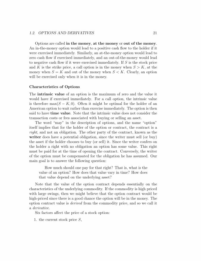
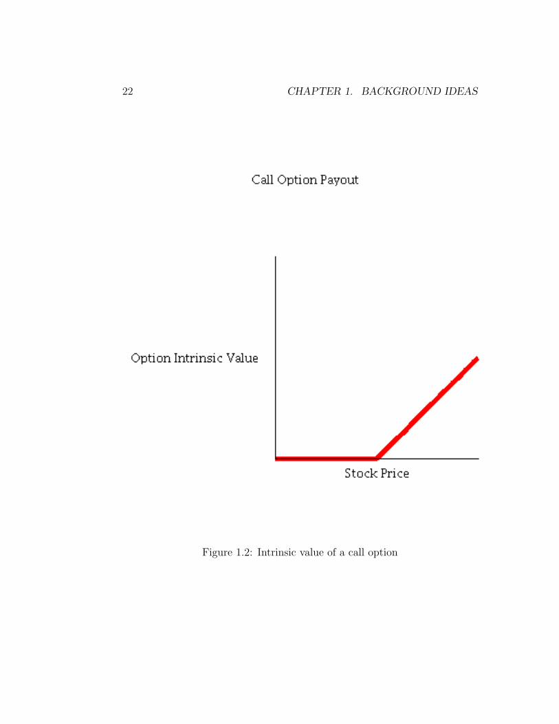
The intrinsic value of an option is the maximum of zero and the value itwould have if exercised immediately. For a call option, the intrinsic valueis therefore max(S − K, 0). Often it might be optimal for the holder of anAmerican option to wait rather than exercise immediately. The option is thensaid to have time value. Note that the intrinsic value does not consider thetransaction costs or fees associated with buying or selling an asset.
The word “may” in the description of options, and the name “option”itself implies that for the holder of the option or contract, the contract is aright, and not an obligation. The other party of the contract, known as thewriter does have a potential obligation, since the writer must sell (or buy)the asset if the holder chooses to buy (or sell) it. Since the writer confers onthe holder a right with no obligation an option has some value. This rightmust be paid for at the time of opening the contract. Conversely, the writerof the option must be compensated for the obligation he has assumed. Ourmain goal is to answer the following question:
How much should one pay for that right? That is, what is thevalue of an option? How does that value vary in time? How doesthat value depend on the underlying asset?
Note that the value of the option contract depends essentially on thecharacteristics of the underlying commodity. If the commodity is high pricedwith large swings, then we might believe that the option contract would behigh-priced since there is a good chance the option will be in the money. Theoption contract value is derived from the commodity price, and so we call ita derivative.
Six factors affect the price of a stock option:
1. the current stock price S,
22 CHAPTER 1. BACKGROUND IDEAS
Figure 1.2: Intrinsic value of a call option

1.2. OPTIONS AND DERIVATIVES 23
2. the strike price K,
3. the time to expiration T − t where T is the expiration time and t is thecurrent time.
4. the volatility of the stock price,
5. the risk-free interest rate,
6. the dividends expected during the life of the option.
Consider what happens to option prices when one of these factors changeswith all the others remain fixed. The results are summarized in the table. Iwill explain only the changes regarding the stock price, the strike price, thetime to expiration and the volatility; the other variables are less importantfor our considerations.
Variable European Call European Put American Call American PutStock Price increases + - + -Strike Price increases - + - +Time to Expiration increases ? ? + +Volatility increases + + + +Risk-free Rate increases + - + -Dividends - + - +
If it is to be exercised at some time in the future, the payoff from a calloption will be the amount by which the stock price exceeds the strike price.Call options therefore become more valuable as the stock price increases andless valuable as the strike price increases. For a put option, the payoff onexercise is the amount by which the strike price exceeds the stock price.Put options therefore behave in the opposite way to call options. Theybecome less valuable as stock price increases and more valuable as strikeprice increases.
Consider next the effect of the expiration date. Both put and call Amer-ican options become more valuable as the time to expiration increases. Theowner of a long-life option has all the exercise options open to the short-life option — and more. The long-life option must therefore, be worth atleast as much as the short-life option. European put and call options do notnecessarily become more valuable as the time to expiration increases. Theowner of a long-life European option can only exercise at the maturity of theoption.
24 CHAPTER 1. BACKGROUND IDEAS
Roughly speaking the volatility of a stock price is a measure of how muchfuture stock price movements may vary relative to the current price. Asvolatility increases, the chance that the stock will either do very well or verypoorly also increases. For the owner of a stock, these two outcomes tendto offset each other. However, this is not so for the owner of a put or calloption. The owner of a call benefits from price increases, but has limiteddownside risk in the event of price decrease since the most that he or she canlose is the price of the option. Similarly, the owner of a put benefits fromprice decreases but has limited upside risk in the event of price increases.The values of puts and calls therefore increase as volatility increases.
Sources
The ideas in this section are adapted from Options, Futures and other Deriva-tive Securities by J. C. Hull, Prentice-Hall, Englewood Cliffs, New Jersey,1993 and The Mathematics of Financial Derivatives by P. Wilmott, S. How-ison, J. Dewynne, Cambridge University Press, 195, Section 1.4, “What areoptions for?”, Page 13 and R. Jarrow and P. Protter, “A short history ofstochastic integration and mathematical finance the early years, 1880–1970”,IMS Lecture Notes, Volume 45, 2004, pages 75–91.
Problems to Work for Understanding
1. (a) Find and write the definition of a “future”, also called a futurescontract. Graph the intrinsic value of a futures contract at itscontract date, or expiration date, as was done for the call option.
(b) Show that holding a call option and writing a put option on thesame asset, with the same strike price K is the same as havinga futures contract on the asset with strike price K. Drawing agraph of the value of the combination and the value of the fu-tures contract together with an explanation will demonstrate theequivalence.
2. Puts and calls are not the only option contracts available, just the mostfundamental and the simplest. Puts and calls are designed to eliminaterisk of up or down price movements in the underlying asset. Someother option contracts designed to eliminate other risks are created ascombinations of puts and calls.

1.3. SPECULATION AND HEDGING 25
(a) Draw the graph of the value of the option contract composed ofholding a put option with strike price K1 and holding a call optionwith strike price K2 where K1 < K2. (Assume both the put andthe call have the same expiration date.) The investor profits onlyif the underlier moves dramatically in either direction. This isknown as a long strangle.
(b) Draw the graph of the value of an option contract composed ofholding a put option with strike price K and holding a call optionwith the same strike price K. (Assume both the put and the callhave the same expiration date.) This is called an long straddle,and also called a bull straddle.
(c) Draw the graph of the value of an option contract composed ofholding one call option with strike price K1 and the simultaneouswriting of a call option with strike price K2 with K1 < K2. (As-sume both the options have the same expiration date.) This isknown as a bull call spread.
(d) Draw the graph of the value of an option contract created by si-multaneously holding one call option with strike price K1, holdinganother call option with strike price K2 where K1 < K2, and writ-ing two call options at strike price (K1 +K2)/2. This is known asa butterfly spread.
(e) Draw the graph of the value of an option contract created byholding one put option with strike price K and holding two calloptions on the same underlying security, strike price, and maturitydate. This is known as a triple option or strap
Outside Readings and Links:
1. What are stock options? An explanation from youtube.com
1.3 Speculation and Hedging
Rating
Student: contains scenes of mild algebra or calculus that may require guid-ance.

26 CHAPTER 1. BACKGROUND IDEAS
Section Starter Question
Discuss examples in your experience of speculation. (Example: think of“scalping tickets”.) A hedge is an investment that is taken out specificallyto reduce or cancel out risk. Discuss examples in your experience of hedges.
Key Concepts
1. Options have two primary uses, speculation and hedging.
2. Options can be a cheap way of exposing a portfolio to a large amountof risk. Sometimes a large amount of risk is desirable. This is the useof options and derivatives for speculation.
3. Options allow the investor to insure against adverse security valuemovements while still benefiting from favorable movements. This isuse of options for hedging. Of course this insurance comes at the costof buying the option.
Vocabulary
1. Speculation is to assume a financial risk in anticipation of a gain,especially to buy or sell in order to profit from market fluctuations.
2. Hedging is to protect oneself financially against loss by a counter-balancing transaction, especially to buy or sell assets as a protectionagainst loss due to price fluctuation.
Mathematical Ideas
Options have two primary uses, speculation and hedging. Consider spec-ulation first.
Example: Speculation on a stock with calls
An investor who believes that a particular stock, say XYZ, is going to risemay purchase some shares in the company. If she is correct, she makesmoney, if she is wrong she loses money. The investor is speculating. Supposethe price of the stock goes from $2.50 to $2.70, then the investor makes $0.20on each $2.50 investment, or a gain of 8%. If the price falls to $2.30, then

1.3. SPECULATION AND HEDGING 27
the investor loses $0.20 on each $2.50 share, for a loss of 8%. These are bothstandard calculations.
Alternatively, suppose the investor thinks that the share price is goingto rise within the next couple of months, and that the investor buys a calloption with exercise price of $2.50 and expiry date in three months’ time.
Now assume that it costs $0.10 to purchase a European call option onstock XYZ with expiration date in three months and strike price $2.50. Thatmeans in three months time, the investor could, if the investor chooses to,purchase a share of XYZ at price $2.50 per share no matter what the currentprice of XYZ stock is! Note that the price of $0.10 for this option may or maynot be an appropriate price for the option, I use $0.10 simply because it iseasy to calculate with. However, 3-month option prices are often about 5% ofthe stock price, so this is reasonable. In three months time if the XYZ stockprice is $2.70, then the holder of the option may purchase the stock for $2.50.This action is called exercising the option. It yields an immediate profit of$0.20. That is, the option holder can buy the share for $2.50 and immediatelysell it in the market for $2.70. On the other hand if in three months time,the XYZ share price is only $2.30, then it would not be sensible to exercisethe option. The holder lets the option expire. Now observe carefully: Bypurchasing an option for $0.10, the holder can derive a net profit of $0.10($0.20 revenue less $0.10 cost) or a loss of $0.10 (no revenue less $0.10 cost.)The profit or loss is magnified to 100% with the same probability of change.Investors usually buy options in quantities of hundreds, thousands, even tensof thousands so the absolute dollar amounts can be quite large. Compared tostocks, options offer a great deal of leverage, that is, large relative changes invalue for the same investment. Options expose a portfolio to a large amountof risk cheaply. Sometimes a large degree of risk is desirable. This is the useof options and derivatives for speculation.
Example: Speculation on a stock with calls
Consider the profit and loss of a investor who buys 100 call options on XYZstock with a strike price of $140. Suppose the current stock price is $138, theexpiration date of the option is two months, and the option price is $5. Sincethe options are European, the investor can exercise only on the expirationdate. If the stock price on this date is less than $140, the investor willclearly choose not to exercise the option since buying a stock at $140 thathas a market value less than $140 is not sensible. In these circumstances the

28 CHAPTER 1. BACKGROUND IDEAS
investor loses the whole of the initial investment of $500. If the stock priceis above $140 on the expiration date, the options will be exercised. Supposefor example,the stock price is $155. By exercising the options, the investor isable to buy 100 shares for $140 per share. If the shares are sold immediately,then the investor makes a gain of $15 per share, or $1500 ignoring transactioncosts. When the initial cost of the option is taken into account, the net profitto the investor is $10 per option, or $1000 on an initial investment of $500.This calculation ignores the time value of money.
Example: Speculation on a stock with puts
Consider an investor who buys 100 European put options on XYZ with astrike price of $90. Suppose the current stock price is $86, the expirationdate of the option is in 3 months and the option price is $7. Since theoptions are European, they will be exercised only if the stock price is below$90 at the expiration date. Suppose the stock price is $65 on this date. Theinvestor can buy 100 shares for $65 per share, and under the terms of the putoption, sell the same stock for $90 to realize a gain of $25 per share, or $2500.Again, transaction costs are ignored. When the initial cost of the option istaken into account, the investor’s net profit is $18 per option, or $1800. Thisis a profit of 257% even though the stock has only changed price $25 froman initial of $90, or 28%. Of course, if the final price is above $90, the putoption expires worthless, and the investor loses $7 per option, or $700.
Example: Hedging with calls on foreign exchange rates
Suppose that a U.S. company knows that it is due to pay 1 million pounds toa British supplier in 90 days. The company has significant foreign exchangerisk. The cost in U.S. dollars of making the payment depends on the exchangerate in 90 days. The company instead can buy a call option contract toacquire 1 million pounds at a certain exchange rate, say 1.7 in 90 days. Ifthe actual exchange rate in 90 days proves to be above 1.7, the companyexercises the option and buys the British pounds it requires for $1,700,000.If the actual exchange rate proves to be below 1.7, the company buys thepounds in the market in the usual way. This option strategy allows thecompany to insure itself against adverse exchange rate increases while stillbenefiting from favorable decreases. Of course this insurance comes at therelatively small cost of buying the option on the foreign exchange rate.
1.3. SPECULATION AND HEDGING 29
Example: Hedging with a portfolio with puts and calls
Since the value of a call option rises when an asset price rises, what happensto the value of a portfolio containing both shares of stock of XYZ and anegative position in call options on XYZ stock? If the stock price is rising,the call option value will also rise, the negative position in calls will becomegreater, and the net portfolio should remain approximately constant if thepositions are held in the right ratio. If the stock price is falling then the calloption value price is also falling. The negative position in calls will becomesmaller. If held in the proper amounts, the total value of the portfolio shouldremain constant! The risk (or more precisely, the variation) in the portfoliois reduced! The reduction of risk by taking advantage of such correlationsis called hedging. Used carefully, options are an indipensable tool of riskmanagement.
Consider a stock currently selling at $100 and having a standard deviationin its price fluctuations of 10%. We can use the Black-Scholes formula derivedlater in the course to show that a call option with a strike price of $100 anda time to expiration of one year would sell for $11.84. A 1 percent rise in thestock from $100 to $101 would drive the option price to $12.73.
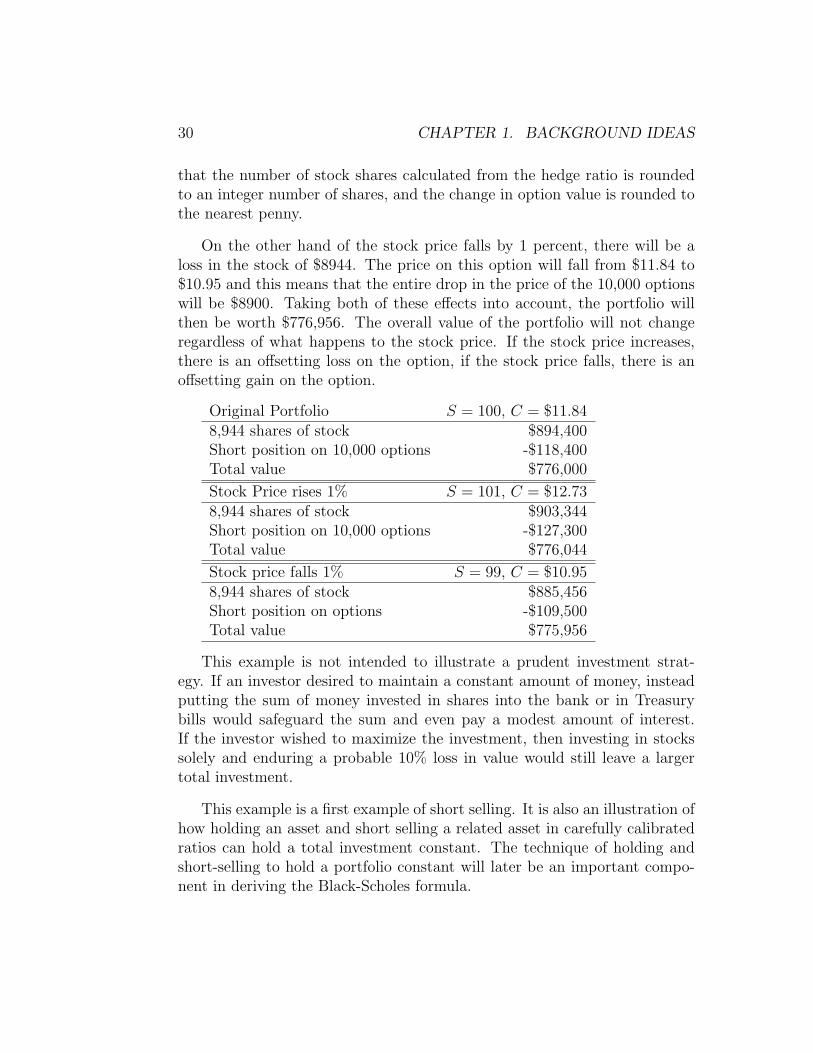
Suppose a trader has an original portfolio comprised of 8944 shares ofstock selling at $100 per share. (The unusual number of 8944 shares will becalculated later from the Black-Scholes formula as a hedge ratio. ) Assumealso that a trader short sells call options on 10,000 shares at the current priceof $11.84. That is, the short seller borrows the options from another traderand must later repay it, creating a negative position in the option value.Once the option is borrowed, the short seller sells it and takes the moneyfrom the sale. The transaction is called short selling because the trader sellsa good he or she does not actually own and must later pay it back. In thetable this short position in the option is indicated by a minus sign. Theentire portfolio of shares and options has a net value of $776,000.
Now consider the effect of a 1 percent change in the price of the stock. Ifthe stock increases 1 percent,the shares will be worth $903,344. The optionprice will increase from $11.84 to $12.73. But since the portfolio also involvesa short position in 10,000 options, this creates a loss of $8,900. This is theadditional value of what the borrowed options are now worth, so it mustadditionally be paid back! After these two effects are taken into account,the value of the portfolio will be $776,044. This is virtually identical to theoriginal value. The slight discrepancy of $44 is rounding error due to the fact
30 CHAPTER 1. BACKGROUND IDEAS
that the number of stock shares calculated from the hedge ratio is roundedto an integer number of shares, and the change in option value is rounded tothe nearest penny.
On the other hand of the stock price falls by 1 percent, there will be aloss in the stock of $8944. The price on this option will fall from $11.84 to$10.95 and this means that the entire drop in the price of the 10,000 optionswill be $8900. Taking both of these effects into account, the portfolio willthen be worth $776,956. The overall value of the portfolio will not changeregardless of what happens to the stock price. If the stock price increases,there is an offsetting loss on the option, if the stock price falls, there is anoffsetting gain on the option.
Original Portfolio S = 100, C = $11.848,944 shares of stock $894,400Short position on 10,000 options -$118,400Total value $776,000
Stock Price rises 1% S = 101, C = $12.738,944 shares of stock $903,344Short position on 10,000 options -$127,300Total value $776,044
Stock price falls 1% S = 99, C = $10.958,944 shares of stock $885,456Short position on options -$109,500Total value $775,956
This example is not intended to illustrate a prudent investment strat-egy. If an investor desired to maintain a constant amount of money, insteadputting the sum of money invested in shares into the bank or in Treasurybills would safeguard the sum and even pay a modest amount of interest.If the investor wished to maximize the investment, then investing in stockssolely and enduring a probable 10% loss in value would still leave a largertotal investment.
This example is a first example of short selling. It is also an illustration ofhow holding an asset and short selling a related asset in carefully calibratedratios can hold a total investment constant. The technique of holding andshort-selling to hold a portfolio constant will later be an important compo-nent in deriving the Black-Scholes formula.

1.3. SPECULATION AND HEDGING 31
Sources
The ideas in this section are adapted from Options, Futures and other Deriva-tive Securities by J. C. Hull, Prentice-Hall, Englewood Cliffs, New Jersey,1993 and The Mathematics of Financial Derivatives by P. Wilmott, S. How-ison, J. Dewynne, Cambridge University Press, 1995, Section 1.4, “What areoptions for?”, Page 13, and Financial Derivatives by Robert Kolb, New YorkInstitute of Finance, New York, 1994, page 110.
Problems to Work for Understanding
1. You would like to speculate on a rise in the price of a certain stock.The current stock price is $29 and a 3-month call with strike of $30costs $2.90. You have $5,800 to invest. Identify two alternative strate-gies, one involving investment in the stock, and the other involvinginvestment in the option. What are the potential gains and losses fromeach?
2. A company knows it is to receive a certain amount of foreign currencyin 4 months. What type of option contract is appropriate for hedging?Please be very specific.
3. The current price of a stock is $94 and 3-month call options with astrike price of $95 currently sell for $4.70. An investor who feels thatthe price of the stock will increase is trying to decide between buying100 shares and buying 2,000 call options. Both strategies involve aninvestment of $9,400. Write and solve an inequality to determine howhigh the stock price must rise for the option strategy to be the moreprofitable. What advice would you give?
Outside Readings and Links:
• Speculation and Hedging A short youtube video on speculation andhedging, from “The Trillion Dollar Bet”.
• More Speculation and Hedging A short youtube video on speculationand hedging.

32 CHAPTER 1. BACKGROUND IDEAS
1.4 Arbitrage
Rating
Student: contains scenes of mild algebra or calculus that may require guid-ance.
Section Starter Question
It’s the day of the big game. You know that your rich neighbor really wantsto buy tickets, in fact you know he’s willing to pay $50 a ticket. While oncampus, you see a hand lettered sign offering “two general-admission ticketsat $25 each, inquire immediately at the mathematics department”. You haveyour phone with you, what should you do? Discuss whether this is a frequentoccurrence, and why or why not? Is this market efficient? Is there any riskin this market?
Key Concepts
1. An arbitrage opportunity is a circumstance where the simultaneous pur-chase and sale of related securities is guaranteed to produce a risklessprofit. Arbitrage opportunities should be rare, but in a world-widemarket they can occur.
2. Prices change as the investors move to take advantage of such an op-portunity. As a consequence, the arbitrage opportunity disappears.This becomes an economic principle: in an efficient market there areno arbitrage opportunities.
3. The basis of arbitrage pricing is that any two investments with identicalpayout streams must have the same price.
Vocabulary
1. Arbitrage is locking in a riskless profit by simultaneously entering intotransactions in two or more markets, exploiting mismatches in pricing.

1.4. ARBITRAGE 33
Mathematical Ideas
The notion of arbitrage is crucial in the modern theory of finance. It is thecornerstone of the Black, Scholes and Merton option pricing theory, devel-oped in 1973, for which Scholes and Merton received the Nobel Prize in 1997(Fisher Black died in 1995).
An arbitrage opportunity is a circumstance where the simultaneous pur-chase and sale of related securities is guaranteed to produce a riskless profit.Arbitrage opportunities should be rare, but on a world-wide basis some dooccur.
This section illustrates the concept of arbitrage with simple examples.
An arbitrage opportunity in exchange rates
Consider a stock that is traded in both New York and London. Suppose thatthe stock price is $172 in New York and £100 in London at a time whenthe exchange rate is $1.7500 per pound. An arbitrageur in New York couldsimultaneously buy 100 shares of the stock in New York and sell them inLondon to obtain a risk-free profit of
100shares× 100£/share× 1.75$/£− 100shares× 172$/share = $300
in the absence of transaction costs. Transaction costs would probably elim-inate the profit on a small transaction like this. However, large investmenthouses face low transaction costs in both the stock market and the foreignexchange market. Trading firms would find this arbitrage opportunity veryattractive and would try to take advantage of it in quantities of many thou-sands of shares.
The shares in New York are underpriced relative to the shares in Londonwith the exchange rate taken into consideration. However, note that thedemand for the purchase of many shares in New York would soon drivethe price up. The sale of many shares in London would soon drive the pricedown. The market would soon reach a point where the arbitrage opportunitydisappears.
An arbitrage opportunity in gold contracts
Suppose that the current market price (called the spot price) of an ounce ofgold is $398 and that an agreement to buy gold in three months time would

34 CHAPTER 1. BACKGROUND IDEAS
set the price at $390 per ounce (called a forward contract). Suppose thatthe price for borrowing gold (actually the annualized 3-month interest ratefor borrowing gold, called the convenience price) is 10%. Additionallyassume that the annualized interest rate on 3-month deposits (such as acertificate of deposit at a bank) is 4%. This set of economic circumstancescreates an arbitrage opportunity. The arbitrageur can borrow one ounce ofgold, immediately sell the borrowed gold at its current price of $398 (thisis called shorting the gold), lend this money out for three months andsimultaneously enter into the forward contract to buy one ounce of gold at$390 in 3 months. The cost of borrowing the ounce of gold is
$398× 0.10× 1/4 = $9.95
and the interest on the 3-month deposit amounts to
$398× 0.04× 1/4 = $3.98.
The investor will therefore have 398.00+3.98−9.95 = 392.03 in the bank ac-count after 3 months. Purchasing an ounce of gold in 3 months, at the forwardprice of $390 and immediately returning the borrowed gold, he will make aprofit of $2.03. This example ignores transaction costs and assumes interestsare paid at the end of the lending period. Transaction costs would probablyconsume the profits in this one ounce example. However, large-volume gold-trading arbitrageurs with low transaction costs would take advantage of thisopportunity by purchasing many ounces of gold.
This transaction can be pictured with the following diagram. Time is onthe horizontal axis, and cash flow is vertical, with the arrow up if cash comesin to the investor, and the arrow down if cash flows out from the investor.
Discussion about arbitrage
Arbitrage opportunities as just described cannot last for long. In the firstexample, as arbitrageurs buy the stock in New York, the forces of supplyand demand will cause the New York dollar price to rise. Similarly as thearbitrageurs sell the stock in London, the London sterling price will be drivendown. The two stock prices will quickly become equivalent at the currentexchange rate. Indeed the existence of profit-hungry arbitrageurs (usuallypictured as frenzied traders carrying on several conversations at once!) makesit unlikely that a major disparity between the sterling price and the dollar

1.4. ARBITRAGE 35
Figure 1.3: A diagram of the cash flow in the gold arbitrage
price could ever exist in the first place. In the second example, once arbi-trageurs start to sell gold at the current price of $398, the price will drop.The demand for the 3-month forward contracts at $390 will cause the priceto rise. Although arbitrage opportunities can arise in financial markets, theycannot last long.
Generalizing, the existence of arbitrageurs means that in practice, onlytiny arbitrage opportunities are observed only for short times in most fi-nancial markets. As soon as sufficiently many observant investors find thearbitrage, the prices quickly change as the investors buy and sell to takeadvantage of such an opportunity. As a consequence, the arbitrage opportu-nity disappears. The principle can stated as follows: in an efficient marketthere are no arbitrage opportunities. In this course, most of our argumentswill be based on the assumption that arbitrage opportunities do not exist,or equivalently, that we are operating in an efficient market.
A joke illustrates this principle very well: A mathematical economist anda financial analyst are walking down the street together. Suddenly each spotsa $100 bill lying in the street at the curb! The financial analyst yells “Wow, a$100 bill, grab it quick!”. The mathematical economist says “Don’t bother, ifit were a real $100 bill, somebody would have picked it up already.” Arbitrageopportunities do exist in real life, but one has to be quick and observant. Forpurposes of mathematical modeling, we can treat arbitrage opportunities as

36 CHAPTER 1. BACKGROUND IDEAS
non-existent as $100 bills lying in the street. It might happen, but we don’tbase our activities on the expectation.
The basis of arbitrage pricing is that any two investments with identicalpayout streams must have the same price. If this were not so, we couldsimultaneously sell the more the expensive instrument and buy the cheaperone; the payment stream from our sale meets the payments for our purchase.We can make an immediate profit.
Before the 1970s most economists approached the valuation of a securityby considering the probability of the stock going up or down. Economistsnow determine the price of a security by arbitrage without the considerationof probabilities. We will use the concept of arbitrage pricing extensively inthis text.
Sources
The ideas in this section are adapted from Options, Futures and other Deriva-tive Securities by J. C. Hull, Prentice-Hall, Englewood Cliffs, New Jersey,1993, Stochastic Calculus and Financial Applications, by J. Michael Steele,Springer, New York, 2001, pages 153–156, the article “What is a . . . FreeLunch” by F. Delbaen and W. Schachermayer, Notices of the AmericanMathematical Society, Vol. 51, Number 5, pages 526–528, and Quantita-tive Modeling of Derivative Securities, by M. Avellaneda and P. Laurence,Chapman and Hall, Boca Raton, 2000.
Problems to Work for Understanding
1. Consider the hypothetical country of Elbonia, where the governmenthas declared a “currency band” policy, in which the exchange ratebetween the domestic currency, the Elbonian Bongo Buck, denoted byEBB, and the US Dollar is guaranteed to fluctuate in a prescribed band,namely:
0.95USD ≤ EBB ≤ 1.05USD
for at least one year. Suppose also that the Elbonian government hasissued 1-year notes denominated in the EBB that pay a continuouslycompounded interest rate of 30%. Assuming that the correspondingcontinuously compounded interest rate for US deposits is 6%, showthat there is an arbitrage opportunity. (Adapted from Quantitative

1.4. ARBITRAGE 37
Modeling of Derivative Securities, by M. Avellaneda and P. Laurence,Chapman and Hall, Boca Raton, 2000, Exercises 1.7.1, page 18).
2. The current exchange rate between the U.S. Dollar and the Euro is1.4280, that is, it costs $1.4280 to buy one Euro. The current 1-yearFed Funds rate, (the bank-to-bank lending rate), in the United Statesis 4.7500% (assume it is compounded continuously). The forward rate(the exchange rate in a forward contract that allows you to buy Eurosin a year) for purchasing Euros 1 year from today is 1.4312. Whatis the corresponding bank-to-bank lending rate in Europe (assume itis compounded continuously), and what principle allows you to claimthat value?
3. According to the article “Bullion bulls” on page 81 in the October 8,2009 issue of The Economist, gold has risen from about $510 per ouncein January 2006 to about $1050 per ounce in October 2009, 46 monthslater.
(a) What is the continuously compounded annual rate of increase ofthe price of gold over this period?
(b) In October 2009, one can borrow or lend money at 5% interest,again assume it compounded continuously. In view of this, de-scribe a strategy that will make a profit in October 2010, involvingborrowing or lending money, assuming that the rate of increase inthe price gold stays constant over this time.
(c) The article suggests that the rate of increase for gold will stayconstant. In view of this, what do you expect to happen to interestrates and what principle allows you to conclude that?
4. Consider a market that has a security and a bond so that money canbe borrowed or loaned at an annual interest rate of r compoundedcontinuously. At the end of a time period T , the security will haveincreased in value by a factor U to SU , or decreased in value by afactor D to value SD. Show that a forward contract with strike pricek that, is, a contract to buy the security which has potential payoffsSU − k and SD − k should have the strike price set at S exp(rT ) toavoid an arbitrage opportunity.
38 CHAPTER 1. BACKGROUND IDEAS
Outside Readings and Links:
1. A lecture on currency arbitrage A link to a youtube video.
1.5 Mathematical Modeling
Rating
Student: contains scenes of mild algebra or calculus that may require guid-ance.
Section Starter Question
Do you believe in the ideal gas law? Does it make sense to “believe in” anequation? What do we really mean when we say we “believe in” an equation?
Key Concepts
1. All mathematical models are wrong, but some mathematical modelsare useful.
2. If the modeling assumptions are satisfied, proper mathematical modelsshould predict well given a wide range of conditions corresponding tothe assumptions.
3. When observed outcomes deviate from predicted ideal behavior in hon-est scientific or engineering work, then we must then alter our assump-tions, re-derive the quantitative relationships, perhaps with more so-phisticated mathematics or introducing more quantities and begin thecycle of modeling again.
Vocabulary
1. A mathematical model is a mathematical structure (often an equa-tion) expressing a relationship among a limited number of quantifiableelements from the “real world” or some isolated portion of it.
1.5. MATHEMATICAL MODELING 39
Mathematical Ideas
Remember the following proverb: All mathematical models are wrong, butsome mathematical models are useful.
Mathematical Modeling
Mathematical modeling involves two equally important activities:
• Building a mathematical structure, a model, based on hypotheses aboutrelations among the quantities that describe the real world situation,and then deriving new relations,
• Evaluating the model, comparing the new relations with the real worldand making predictions from the model.
Good mathematical modeling explains the hypotheses, the development ofthe model and its solutions, and then supports the findings by comparingthem mathematically with the actual circumstances. Successful modelingrequires a balance between so much complexity that making predictions fromthe model may be intractable and so little complexity that the predictionsare unrealistic and useless. A successful model must allow a user to considerthe effects of different policies.
At a more detailed level, mathematical modeling involves successive stepsin the cycle of modeling:
1. Factors and observations,
2. Mathematical structure,
3. Testing and sensitivity analysis,
4. Effects and observations.
Consider the diagram in Figure 1.4 which illustrates the cycle of modeling.Steps 1 and 2 in the more detailed cycle are the first activity described aboveand steps 3 and 4 are the second activity.

40 CHAPTER 1. BACKGROUND IDEAS
Figure 1.4: The cycle of modeling
1.5. MATHEMATICAL MODELING 41
Modeling
A good description of the model will begin with an organized and completedescription of important factors and observations. The description will oftenuse data gathered from observations of the problem. It will also include thestatement of scientific laws and relations that apply to the important factors.From there, the model must summarize and condense the observations intoa small set of hypotheses that capture the essence of the observations. Thesmall set of hypotheses is a restatement of the problem, changing the problemfrom a descriptive, even colloquial, question into a precise formulation thatmoves the statement from the general to the specific. This sets the stage forthe modeler to demonstrate a clear link between the listed assumptions andthe building of the model.
The hypotheses translate into a mathematical structure that becomes theheart of the mathematical model. Many mathematical models, particularlythose from physics and engineering, become a single equation but mathe-matical models need not be a single concise equation. Mathematical modelsmay be a regression relation, either a linear regression, an exponential re-gression or a polynomial regression. The choice of regression model shouldexplicitly follow from the hypotheses since the growth rate is an importantconsequence of the observations. The mathematical model may be a linear ornonlinear optimization model, consisting of an objective function and a setof constraints. Again the choice of linear or nonlinear functions for the ob-jective and constraints should explicitly follow from the nature of the factorsand the observations. For dynamic situations, the observations often involvesome quantity and its rates of change. The hypotheses express some con-nection between these quantities and the mathematical model then becomesa differential equation, either linear or nonlinear depending on the explicitdetails of the scientific laws relating the factors considered. For discretelysampled data instead of continuous time expressions the model may becomea difference equation. If an important feature of the observations and factorsis noise or randomness, then the model may be a probability distribution ora stochastic process. The classical models from science and engineering usu-ally take one of these classical equation-like forms but not all mathematicalmodels need to follow this format. Models may be a connectivity graph, ora group of transformations.
If the number of variables is more than a few, or the relations are compli-cated to write in a concise mathematical expression then the model can be a

42 CHAPTER 1. BACKGROUND IDEAS
computer program. Programs written in either high-level languages such asC, FORTRAN or Basic and very-high-level languages such as MATLAB or acomputer algebra system are mathematical models. Spreadsheets combiningthe data and the calculations are a popular and efficient way to construct amathematical model. The collection of calculations in the spreadsheet ex-press the laws connecting the factors which are represented by the data inthe rows and columns of the spreadsheet. Some mathematical models maybe expressed by using more elaborate software specifically designed for mod-eling. Some software allows the user to describe the connections betweenfactors graphically to create and alter a model.
Although this set of examples of mathematical models varies in theoreticalsophistication and the equipment used, the core of each is to connect the dataand the relations into a mechanism that allows the user to vary elementsof the model. Creating a model, whether a single equation, a complicatedmathematical structure, a quick spreadsheet, or a large program is the essenceof the first step connecting the boxes labeled 1 and 2 above.
First models need not be sophisticated or detailed. For beginning anal-ysis “back of the envelope calculations” and “dimensional analysis” will beas effective as spending time setting up an elaborate model or solving equa-tions with advanced mathematics. Unit analysis to check consistency andoutcomes of relations is important to check the harmony of the modelingassumptions. A good model pays attention to units, the quantities should besensible and match. Even more important, a non-dimensionalizized modelreveals significant relationships, and major influences. Unit analysis is animportant part of modeling, and goes far beyond simple checking to makesure “units cancel.” [34, 32]
Mathematical Solution
Once the modelers have created the model, then they should derive somenew relations among the important quantities selected to describe the realworld situation. This is the step connecting the boxes labeled 2 and 3 in thediagram. If the model is an equation, for instance the Ideal Gas Law, thenone can solve the equation for one of the variables in terms of the others.In the Ideal Gas Law, solving for one of the gas parameters is quite easy.A regression equation model may require almost no mathematical solution,although it might be useful to find auxiliary quantities such as rates of growthor maxima or minima. For an optimization problem the solution is the set of

1.5. MATHEMATICAL MODELING 43
optima or the rates of change of optima with respect to the constraints. If themodel is a differential equation or a difference equation, then the solution mayhave some mathematical substance. For instance, for a ballistics problem, themodel may be a differential equation and the solution by calculus methodsyields the equation of motion. For a problem with randomness, the derivationmay find the mean or the variance. For a connectivity graph, one might beinterested in the number of cycles, components or the diameter of the graph.If the model is a computer program, then this step usually involves runningthe program to obtain the output.
It is easy for students to focus most attention on this stage of the process,since the usual methods are the core of the typical mathematical curriculum.This step usually requires no interpretation, the model dictates the methodsthat must be used. This step is often the easiest in the sense that it is theclearest on how to proceed, although the mathematical procedures may bedaunting.
Testing and Sensitivity
Once this step is done, the model is ready for testing and sensitivity analysis.This is the step that connects the boxes labeled 3 and 4. At the least,the modelers should try to verify, even with common sense, the results ofthe solution. Typically for a mathematical model, the previous step allowsthe modelers to produce some important or valuable quantity of the model.Modelers compare the results of the model with standard or common inputswith known quantities for the data or statement of the problem. This maybe as easy as substituting into the derived equation, regression expression, orequation of motion. When running a computer model or program, this mayinvolve sequences of program runs and related analysis. With any model,the results will probably not be exactly the same as the known data sointerpretation or error analysis will be necessary. The interpretation willtake judgment on the relative magnitudes of the quantities produced in lightof the confidence in the exactness or applicability of the hypotheses.
Another important activity at this stage in the modeling process is thesensitivity analysis. The modelers should choose some critical feature of themodel and then vary the parameter value that quantifies that feature. Theresults should be carefully compared to the real world and to the predictedvalues. If the results do not vary substantially, then perhaps the feature orparameter is not as critical as believed. This is important new information
44 CHAPTER 1. BACKGROUND IDEAS
for the model. On the other hand, if a predicted or modeled value variessubstantially in comparison to the parameter as it is slightly varied, thenthe accuracy of measurement of the critical parameter assumes new impor-tance. In sensitivity analysis, just as in all modeling, this comparison of“varying substantially” should be measured with significant digits, relativemagnitudes, and rates of change. Here is another area where expressing pa-rameters in dimensionless groups is important [34]. In some areas of appliedmathematics such as linear optimization and statistics, a side effect of thesolution method is that it produces sensitivity parameters. In linear opti-mization, these are sometimes called the shadow prices and these additionalsolution values should be used whenever possible.
Interpretation and Refinement
Finally the modelers must take the results from the previous steps and usethem to refine the interpretation and understanding of the real world situ-ation. This interpretation step is represented in the diagram by connectionbetween the boxes labeled 4 and 1, completing the cycle of modeling. Forexample, if the situation is modeling motion, then examining results mayshow that the predicted motion is faster than measured, or that the objectdoes not travel as far as the model predicts. Then it may be that the modeldoes not include the effects of friction, and so friction should be incorporatedinto a new model. At this step, the modeler has to be open and honest inassessing the strengths and weaknesses of the model. It also requires an im-proved understanding of the real world situation to include the correct newelements and hypotheses to correct the discrepancies in the results.
The step between stages 4 and 1 may suggest new processes, or experi-mental conditions to alter the model. If the problem suggests changes thenthose changes should be implemented and tested in another cycle in themodeling process.
A good summary of the modeling process is that it is an intense andstructured application of “critical thinking”. Sophistication of mathematicaltechniques is not always necessary, the mathematics connecting steps 2 and3 or potentially steps 3 and 4 may only be arithmetic. The key to goodmodeling is the critical thinking that occurs between steps 1 and 2, steps 3and 4, and 4 and 1. If a model does not fit into this paradigm, it probablydoes not meet the criteria for a good model.
Good mathematical modeling, like good critical thinking, does not arise

1.5. MATHEMATICAL MODELING 45
automatically or naturally. The craft of creating, solving, using, and in-terpreting a mathematical model must be practiced and developed. Thestructured approach to modeling helps distinguish the distinct steps, eachrequiring separate intellectual skills. It also provides a framework for devel-oping and explaining a mathematical model.
An example from physical chemistry
This section illustrates the cycle of mathematical modeling with a simpleexample from physical chemistry. This simple example provides us with apowerful analogy about the role of mathematical modeling in mathematicalfinance. I have slightly modified the historical order of discovery to illustratethe idealized modeling cycle. Scientific progress rarely proceeds in such adirect line.
Scientists observed that diverse gases such as air, water vapor, hydrogen,and carbon dioxide all behave predictably and similarly. After many obser-vations, scientists derived empirical relations such as Boyle’s law, and thelaw of Charles and Gay-Lussac about the gas. These laws express relationsamong the volume V , the pressure P , the amount n, and the temperature.T of the gas.
In classical theoretical physics, we can define an ideal gas by making thefollowing assumptions [19]:
1. A gas consists of particles called molecules which have mass, but es-sentially have no volume, so the molecules occupy a negligibly smallfraction of the volume occupied by the gas.
2. The molecules can move in any direction with any speed.
3. The number of molecules is large.
4. No appreciable forces act on the molecules except during a collision.
5. The collisions between molecules and the container are elastic, andof negligible duration so both kinetic energy and momentum are con-served.
6. All molecules in the gas are identical.

46 CHAPTER 1. BACKGROUND IDEAS
From this limited set of assumptions about theoretical entities calledmolecules physicists can derive the equation of state for an ideal gas in termsof the 4 quantifiable elements of volume, pressure, amount, and temperature.The equation of state or ideal gas law is
PV = nRT.
where R is a measured constant, called the universal gas constant. This givesa simple algebraic equation relating the 4 quantifiable elements describing agas. The equation of state or ideal gas law predicts very well the properties ofgases under the wide range of pressures, temperatures, masses and volumescommonly experienced in everyday life. The ideal gas law predicts withaccuracy necessary for safety engineering the pressure and temperature incar tires and commercial gas cylinders. This level of prediction works evenfor gases we know do not satisfy the assumptions, such as air, which chemistrytells us is composed of several kinds of molecules which have volume and donot experience completely elastic collisions because of intermolecular forces.We know the mathematical model is wrong, but it is still useful.
Nevertheless, scientists soon discovered that the assumptions of an idealgas predict that the difference in the constant-volume specific heat and theconstant-pressure specific heat of gases should be the same for all gases, aprediction that scientists observe to be false. The simple ideal gas theoryworks well for monatomic gases, such as helium, but does not predict so wellfor more complex gases. This scientific observation now requires additionalassumptions, specifically about the shape of the molecules in the gas. Thederivation of the relationship for the observable in a gas is now more complex,requiring more mathematical techniques.
Moreover, under extreme conditions of low temperatures or high pres-sures, scientists observe new behaviors of gases. The gases condense intoliquids, pressure on the walls drops and the gases no longer behave accordingto the relationship predicted by the ideal gas law. We cannot neglect thesedeviations from ideal behavior in accurate scientific or engineering work. Wenow have to admit that under these extreme circumstances we can no longerignore the size of the molecules, which do occupy some appreciable volume.We also must admit that intermolecular forces must be considered. The twoeffects just described can be incorporated into a modified equation of stateproposed by J.D. van der Waals in 1873. Van der Waals’ equation of stateis: (
P +na
V 2
)(V − b) = RT

1.5. MATHEMATICAL MODELING 47
The additional constants a and b represent the new elements of intermolecularattraction and volume effects respectively. If a and b are small because we areconsidering a monatomic gas under ordinary conditions, the Van der Waalsequation of state can be well approximated by the ideal gas law. Otherwisewe must use this more complicated relation for engineering our needs withgases.
It is now realized that because of the complex nature of the intermolecu-lar forces, a real gas cannot be rigorously described by any simple equationof state. It can be honestly said that the assumptions of the ideal gas arenot correct, yet are sometimes useful. Likewise, the predictions of the vander Waals equation of state describe quite accurately the behavior of carbondioxide gas in appropriate conditions. Yet for very low temperatures, carbondioxide deviates from even these modified predictions because we know thatthe van der Waals model of the gas is wrong. Even this improved mathe-matical model is wrong, but it still is useful.
Later we will make a limited number of idealized assumptions about se-curities markets. We start from empirical observations of economists aboutsupply and demand and the role of prices as a quantifiable element relatingthem. We will ideally assume that
1. a very large number of identical, rational traders,
2. all traders always have complete information about all assets they aretrading,
3. prices may be random, but are continuous with some probability dis-tribution,
4. trading transactions take negligible time,
5. trading transactions can be made in any amounts.
These assumptions are very similar to the assumptions about an ideal gas.From the assumptions we will be able to make some standard economicarguments to derive some interesting relationships about option prices. Theserelationships can help us manage risk, and speculate intelligently in typicalmarkets. However, caution is necessary. In discussing the economic collapseof 2008-2009, blamed in part on the overuse or even abuse of mathematicalmodels of risk, Valencia [51] says “Trying ever harder to capture risk inmathematical formulae can be counterproductive if such a degree of accuracy
48 CHAPTER 1. BACKGROUND IDEAS
is intrinsically unobtainable.” If the dollar amounts get very large (so thatrationality no longer holds!), or only a few traders are involved, or sharpjumps in prices occur, or the trades come too rapidly for information tospread effectively, we must proceed with caution. The observed financialoutcomes may deviate from predicted ideal behavior in accurate scientific oreconomic work, or financial engineering.
We must then alter our assumptions, re-derive the quantitative relation-ships, perhaps with more sophisticated mathematics or introducing morequantities and begin the cycle of modeling again.
Sources
Some of the ideas about mathematical modeling are adapted from the articleby Valencia [51] and the book When Genius Failed by Roger Lowenstein.
Problems to Work for Understanding
Outside Readings and Links:
1. Duke University Modeling Contest Team Accessed August 29, 2009
1.6 Randomness
Rating
Student: contains scenes of mild algebra or calculus that may require guid-ance.
Section Starter Question
When we say something is “random”, what do we mean? What is the dic-tionary definition of “random”?
Key Concepts
1. Assigning probability 1/2 to the event that a coin will land heads andprobability 1/2 to the event that a coin will land tails is a mathematical
1.6. RANDOMNESS 49
model that summarizes our experience with many coins. In the contextof statistics, this is called the frequentist approach to probability.
2. A coin flip is a deterministic physical process, subject to the physicallaws of motion. Extremely narrow bands of initial conditions determinethe outcome of heads or tails. The assignment of probabilities 1/2 toheads and tails is a summary measure of all initial conditions thatdetermine the outcome precisely.
3. The Random Walk Theory of asset prices claims that market pricesfollow a random path, without any influence by past price movements.This theory says it is impossible to predict which direction the marketwill move at any point, especially in the short term. More refined ver-sions of the random walk theory postulate a probability distributionfor the market price movements. In this way, the random walk theorymimics the mathematical model of a coin flip, substituting a probabil-ity distribution of outcomes for the ability to predict what will reallyhappen.
Vocabulary
1. Technical analysis claims to predict security prices by relying onthe assumption that market data, such as price, volume, and patternsof past behavior can help predict future (usually short-term) markettrends.
2. The Random Walk Theory of the market claims that market pricesfollow a random path up and down according to some probability dis-tribution without any influence by past price movements. This assump-tion means that it is not possible to predict which direction the marketwill move at any point, although the probability of movement in a givendirection can be calculated.
Mathematical Ideas
Coin Flips and Randomness
The simplest, most common, and in some ways most fundamental exampleof a random process is a coin flip. We flip a coin, and it lands one side up.

50 CHAPTER 1. BACKGROUND IDEAS
We assign the probability 1/2 to the event that the coin will land heads andprobability to 1/2 to the event that the coin will land tails. But what doesthat assignment of probabilities really express?
To assign the probability 1/2 to the event that the coin will land headsand probability 1/2 to the event that the coin will land tails is a mathe-matical model that summarizes our experience with many coins. We haveflipped many coins many times, and we observe that about half the time thecoin comes up heads, and about half the time the coin comes up tails. Sowe abstract this observation to a mathematical model containing only oneparameter, the probability of a heads. In the context of statistics, this iscalled the frequentist approach to probability.
From this simple model of the outcome of a coin flip, we can derivesome mathematical consequences. We will do this extensively in the chapteron coin-flipping. One of the first consequences we can derive is called theWeak Law of Large Numbers. This consequence will reassure us that if wemake the probability assignment based on the frequentist approach, thenthe long term observations with the assignment will match our expectations.The mathematical model shows its worth by making definite predictions offuture outcomes. We will demonstrate other more sophisticated theorems,some with expected consequences, others are surprising. Observations showthe predictions generally match experience with real coins, and so this simplemathematical model has value in explaining and predicting coin flip behavior.In this way, the simple mathematical model is satisfactory.
In other ways, the probability approach is unsatisfactory. A coin flip isa physical process, subject to the physical laws of motion. The renownedapplied mathematician J. B. Keller investigated coin flips in this way. Heassumed a circular coin with negligible thickness flipped from a given heighty0 = a > 0, and considered its motion both in the vertical direction underthe influence of gravity, and its rotational motion imparted by the flip untilit lands on the surface y = 0. The initial conditions imparted to the coinflip are the initial upward velocity and the initial rotational velocity. Undersome additional simplifying assumptions Keller shows that the fraction offlips which land heads approaches 1/2 if the initial vertical and rotationalvelocities are high enough. Actually, Keller shows more, that for high initialvelocities there are very narrow bands of initial conditions which determinethe outcome of heads or tails. From Keller’s analysis we see that the random-ness comes from the choice of initial conditions. Because of the narrownessof the bands of initial conditions, very slight variations of initial upward ve-

1.6. RANDOMNESS 51
locity and rotational velocity lead to different outcomes. The assignment ofprobabilities 1/2 to heads and tails is actually a statement of the measure ofthe initial conditions that determine the outcome precisely.
The assignment of probabilities 1/2 to heads and tails is actually a state-ment of our inability to measure the initial conditions and the dynamicsprecisely. These initial conditions alternate in adjacent narrow regions, sowe cannot accurately distinguish among them. We instead measure the wholeproportion of initial conditions leading to each outcome.
If the coin lands on a hard surface and bounces the physical predictionof outcomes is now almost impossible, because we know even less about thedynamics of the bounce, let alone the new initial conditions imparted by thebounce.
Another mathematician who often collaborated with J. B. Keller, PersiDiaconis, has exploited this determinism. Diaconis, an accomplished magi-cian, is reportedly able to flip many heads in a row using his manual skill.Moreover, he has worked with mechanical engineers to build a precise coin-flipping machine that can flip many heads in a row by controlling the initialconditions precisely. The illustration is a picture of such a machine.
Mathematicians Diaconis, Susan Holmes and Richard Montgomery havedone an even more detailed analysis of the physics of coin flips. There is aslight physical bias favoring the coin’s initial position 51% of the time. Thebias results from the rotation of the coin around three axes of rotation atonce. Their more complete dynamical description of coin flipping needs moreinitial information since the coin-flipping machines help to show that flippingphysical coins is actually slightly biased.
If the coin bounces or rolls the physics becomes more complicated. Thisis particularly true if the coin is allowed to roll on one edge upon landing.The edges of coins are often milled with a slight taper, so the coin is reallymore conical than cylindrical. When landing on edge or spinning, the coinwill tip in the tapered direction.
The assignment of a reasonable probability to a coin toss both summarizesand hides our inability to measure the initial conditions precisely and tocompute the physical dynamics easily. The probability assignment is usuallya good enough model, even if wrong. Except in circumstances of extremeexperimental care with many measurements, the proportion of heads can betaken to be 1/2.
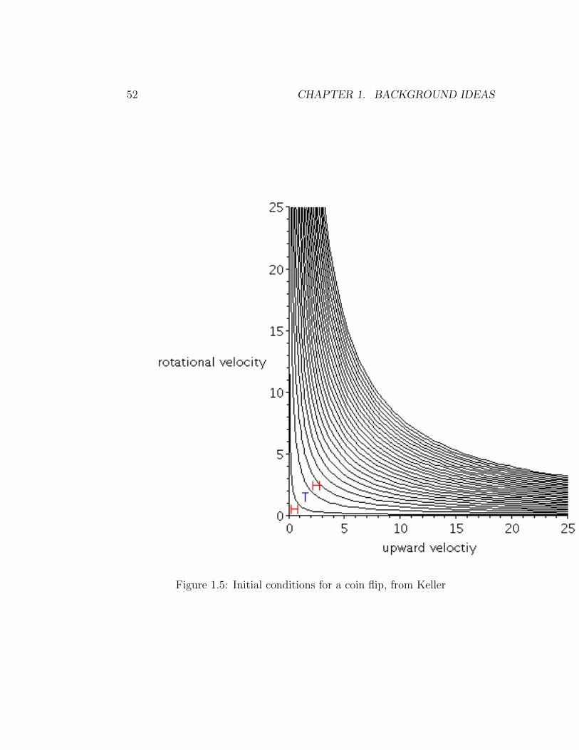
52 CHAPTER 1. BACKGROUND IDEAS
Figure 1.5: Initial conditions for a coin flip, from Keller

1.6. RANDOMNESS 53
Figure 1.6: Persi Diaconis’ mechanical coin flipper
Randomness and the Markets
A branch of financial analysis, generally called technical analysis, claims tobe able to predict security prices by relying on the assumption that marketdata, such as price, volume, and patterns of past behavior can help predictfuture (usually short-term) market trends. Technical analysis also usuallyassumes that market psychology influences trading in a way that enablespredicting when a stock will rise or fall.
In contrast is random walk theory. This theory claims that marketprices follow a random path without influence by past price movements. Therandomness makes it impossible to predict which direction the market willmove at any point, especially in the short term. More refined versions of therandom walk theory postulate a probability distribution for the market pricemovements. In this way, the random walk theory mimics the mathematicalmodel of a coin flip, substituting a probability distribution of outcomes forthe ability to predict what will really happen.
If the coin flip, although deterministic and ultimately simple in executioncannot be practically predicted with well-understood physical principles, thenit should be hard to believe that market dynamics can be predicted. Mar-ket dynamics are based on the interactions of thousands of variables and
54 CHAPTER 1. BACKGROUND IDEAS
the actions of thousands of people. The economic principles at work on thevariables are understood in only fundamental ways in contrast to physicalprinciples. Much less understood are the psychological principles that moti-vate people to buy or sell at a specific price and time. Even allowing thatmarket prices are determined by principles which might be mathematicallyexpressed as unambiguously as the Lagrangian dynamics of the coin flip,that still leaves the precise determination of the initial conditions and theparameters.
It is more practical to admit our inability to predict using basic principlesand to instead use a probability distribution to describe what we observe.In this text, we use the random walk theory with minor modifications andqualifications. We will see that random walk theory does good job of leadingto predictions that can be tested against evidence, just as a coin-flip sequencecan be tested against the classic limit theorems of probability. In certaincases, with extreme care, special tools and many measurements of data wemay be able to discern biases, even predictability in markets. This does notinvalidate the utility of the less precise first-order models that we build andinvestigate. All models are wrong, but some models are useful.
The cosmologist Stephen Hawking says in his book A Brief History ofTime [20] “A theory is a good theory if it satisfies two requirements: it mustaccurately describe a large class of observations on the basis of a model thatcontains only a few arbitrary elements, and it must make definite predictionsabout the results of future observations.” As we will see the random walktheory of markets does both. Unfortunately, technical analysis typically failsthe first in that it usually does not describe a large class of observations andusually contains many arbitrary elements.
True Randomness
The outcome of a coin flip is physically determined. The numbers generatedby an “random-number-generator” algorithm are deterministic, and are moreproperly known as pseudo-random numbers. The movements of prices in amarket are governed by the hopes and fears of presumably rational humanbeings, and so might in principle be predicted. For each of these, we substi-tute a probability distribution of outcomes as a sufficient summary of whatwe have experienced in the past but are unable to predict precisely.
Does true randomness exist anywhere? Yes, in the quantum world ofatoms. For example, the time until the radioactive disintegration of a spe-

1.7. STOCHASTIC PROCESSES 55
cific N-13 atom to a C-13 isotope is apparently truly random, since it seemswe fundamentally cannot determine when it will occur by calculating somephysical process underlying the disintegration. Scientists must use probabil-ity theory to describe the physical processes associated with true quantumrandomness.
Einstein found this quantum theory hard to accept. His famous remarkis that “God does not play at dice with the universe.” Nevertheless, ex-periments have confirmed the true randomness of quantum processes. Someresults combining quantum theory and cosmology imply even more profoundand bizarre results. Again in the words of Stephen Hawking, “God not onlyplays dice. He also sometimes throws the dice where they cannot be seen.”
Sources
This section is adapted from: “The Probability of Heads”, by J. B. Keller,American Mathematical Monthly, Volume 83, Number 3, March 1986, pages191–197, and definitions from investorwords.com. See also the article “AReliable Randomizer, Turned on Its Head”, David Adler, Washington Post,August 2, 2009.
Problems to Work for Understanding
Outside Readings and Links:
1. A satire on the philosophy of randomness Accessed August 29, 2009.
1.7 Stochastic Processes
Rating
Student: contains scenes of mild algebra or calculus that may require guid-ance.
Section Starter Question
Name something that is both random and varies over time. Does the ran-domness depend on the history of the process or only on its current state?
56 CHAPTER 1. BACKGROUND IDEAS
Key Concepts
1. A sequence or interval of random outcomes, that is to say, a stringof random outcomes dependent on time as well as the randomnessis called a stochastic process. Because of the inclusion of a timevariable, the rich range of random outcome distributions is multipliedto an almost bewildering variety of stochastic processes. Nevertheless,the most commonly studied types of random processes do have a familytree of relationships.
2. Stochastic processes are functions of two variables, the time index andthe sample point. As a consequence, there are several ways to repre-sent the stochastic process. The simplest is to look at the stochasticprocess at a fixed value of time. The result is a random variable witha probability distribution, just as studied in elementary probability.
3. Another way to look at a stochastic process is to consider the stochas-tic process as a function of the sample point ω. For each ω there is anassociated function of time X(t). This means that one can look at astochastic process as a mapping from the sample space Ω to a set offunctions. In this interpretation, stochastic processes are a generaliza-tion from the random variables of elementary probability theory.
Vocabulary
1. A sequence or interval of random outcomes, that is, random outcomesdependent on time is called a stochastic process.
2. Let J be a subset of the non-negative real numbers. Let Ω be a set,usually called the sample space or probability space. An elementω of Ω is called a sample point or sample path. Let S be a set ofvalues, often the real numbers, called the state space. A stochasticprocess is a function X : (J,Ω) → S, that is a function of both timeand the sample point to the state space.
3. The particular stochastic process usually called a simple randomwalk Tn gives the position in the integers after taking a step to theright for a head, and a step to the left for a tail.
1.7. STOCHASTIC PROCESSES 57
4. A generalization of a Markov chain is a Markov Process. In a Markovprocess, we allow the index set to be either a discrete set of times asthe integers or an interval, such as the non-negative reals. Likewise thestate space may be either a set of discrete values or an interval, eventhe whole real line. In mathematical notation a stochastic process X(t)is called Markov if for every n and t1 < t2 < . . . < tn and real numberxn, we have
P [X(tn) ≤ xn|X(tn−1), . . . , X(t1)] = P [X(tn) ≤ xn|X(tn−1)] .
Many of the models we use in this text will naturally be taken asMarkov processes because of the intuitive appeal of this “memory-less”property.
Mathematical Ideas
Definition and Notations
A sequence or interval of random outcomes, that is, random outcomes de-pendent on time is called a stochastic process. Stochastic is a synonym for“random.” The word is of Greek origin and means “pertaining to chance”(Greek stokhastikos, skillful in aiming; from stokhasts, diviner; from stok-hazesthai, to guess at, to aim at; and from stochos target, aim, guess). Themodifier stochastic indicates that a subject is viewed as random in some as-pect. Stochastic is often used in contrast to “deterministic,” which meansthat random phenomena are not involved.
More formally, let J be subset of the non-negative real numbers. UsuallyJ is the natural numbers 0, 1, 2, . . . or the non-negative reals t : t ≥ 0. Jis the index set of the process, and we usually refer to t ∈ J as the timevariable. Let Ω be a set, usually called the sample space or probabilityspace. An element ω of Ω is called a sample point or sample path. LetS be a set of values, often the real numbers, called the state space. Astochastic process is a function X : (J,Ω) → S, a function of both timeand the sample point to the state space.
Because we are usually interested in the probability of sets of samplepoints that lead to a set of outcomes in the state space and not the individualsample points, the common practice is to suppress the dependence on thesample point. That is, we usually write X(t) instead of the more completeX(t, ω). Furthermore, if the time set is discrete, say the natural numbers,
58 CHAPTER 1. BACKGROUND IDEAS
then we usually write the index variable or time variable as a subscript.Thus Xn would be the usual notation for a stochastic process indexed by thenatural numbers and X(t) is a stochastic process indexed by the non-negativereals. Because of the randomness, we can think of a stochastic process asa random sequence if the index set is the natural numbers and a randomfunction if the time variable is the non-negative reals.
Examples
The most fundamental example of a stochastic process is a coin flip sequence.The index set is the set of counting numbers, counting the number of the flip.The sample space is the set of all possible infinite coin flip sequences Ω =HHTHTTTHT . . . , THTHTTHHT . . . , . . .. We take the state space tobe the set 1, 0 so that Xn = 1 if flip n comes up heads, and Xn = 0 if the flipcomes up tails. Then the coin flip stochastic process can be viewed as the setof all “random” sequences of 1’s and 0’s. An associated random process is totake Sn =
∑nj=1Xj. Now the state space is the set of natural numbers. The
stochastic process Sn counts the number of heads encountered in the flippingsequence up to flip number n.
Alternatively, we can take the same index set, the same probability spaceof coin flip sequences and define Yn = 1 if flip n comes up heads, and Yn = −1if the flip comes up tails. This is just another way to encode the coin flipsnow as random sequences of 1’s and −1’s. A more interesting associatedrandom process is to take Tn =
∑nj=1 Yj. Now the state space is the set of
integers. The stochastic process Tn gives the position in the integers aftertaking a step to the right for a head, and a step to the left for a tail. Thisparticular stochastic process is usually called a simple random walk. Wecan generalize random walk by allowing the state space to be the set of pointswith integer coordinates in two-, three- or higher-dimensional space, calledthe integer lattice.
Markov Chains
A Markov chain is sequence of random variables Xj where the index jruns through 0, 1, 2, . . .. The sample space is not specified explicitly, but itinvolves a sequence of random selections detailed by the effect in the statespace. The state space can be either a finite or infinite set of discrete states.
1.7. STOCHASTIC PROCESSES 59
The defining property of a Markov chain is that
P [Xj = l|X0 = k0, X1 = k1, . . . , Xj−1 = kj−1] = P [Xj = l|Xj−1 = kj−1] .
In words, the future is conditionally independent of the past, the probabilityof transition from state kj−1 at time j − 1 to state l at time j depends onlyon kj−1 and l, not on the history X0 = k0, X1 = k1, . . . , Xj−2 = kj−2 of howthe process got to kj−1
A simple random walk is an example of a Markov chain. The states arethe integers and the transition probabilities are
P [Xj = l|Xj−1 = k] = 1/2 if l = k − 1 or l = k + 1
P [Xj = l|Xj−1 = k] = 0 otherwise
Another example would be the position of a game piece in the boardgame Monopoly. The index set is the counting numbers listing the playsof the game. The sample space is the set of infinite sequence of rolls of apair of dice. The state space is the set of 40 real-estate properties and otherpositions around the board.
Markov chains have been extended to making optimal decisions underuncertainty as “Markov decision processes”. Another extension to signal pro-cessing and bioinformatics is called “hidden Markov models”. Markov chainsare an important and useful class of stochastic processes. Mathematicianshave extensively studied and classified Markov chains and their extensionsbut we will not have reason to examine them carefully in this text.
A generalization of a Markov chain is a Markov process. In a Markovprocess, we allow the index set to be either a discrete set of times as theintegers or an interval, such as the non-negative reals. Likewise the statespace may be either a set of discrete values or an interval, even the wholereal line. In mathematical notation a stochastic process X(t) is called Markovif for every n and t1 < t2 < . . . < tn and real number xn, we have
P [X(tn) ≤ xn|X(tn−1), . . . , X(t1)] = P [X(tn) ≤ xn|X(tn−1)] .
Many of the models we use in this text will naturally be taken as Markovprocesses because of the intuitive appeal of this “memory-less” property.
Many stochastic processes are naturally expressed as taking place in adiscrete state space with a continuous time index. For example, consider ra-dioactive decay, counting the number of atomic decays which have occurred
60 CHAPTER 1. BACKGROUND IDEAS
up to time t by using a Geiger counter. The discrete state variable is thecounting number of clicks heard. The mathematical “Poisson process” is anexcellent model of this physical process. More generally, instead of radioac-tive events giving a single daughter particle, we can imagine a birth eventwith a random number (distributed according to some probability law) ofoffspring born at random times. Then the stochastic process measures thepopulation in time. These are called “birth processes” and make excellentmodels in population biology and the physics of cosmic rays. We can con-tinue to generalize and imagine that each individual in the population hasa random life-span distributed according to some law, then dies. This givesa “birth-and-death process”. In another variation, we can imagine a dis-ease with a random number of susceptibles getting infected, in turn infectinga random number of others, then recovering and becoming immune. Thestochastic process counts how many of each type there are at any time, an“epidemic process”.
In another variation, we can consider customers arriving at a servicecounter at random intervals with some specified distribution, often taken tobe an exponential probability distribution with parameter λ. The customersare served one-by-one, each taking a random service time, again often takento be exponentially distributed. The state space is the number of customerswaiting to be served, the queue length at any time. These are called “queuingprocesses”. Mathematically, many of these processes can be studied by whatare called “compound Poisson processes”.
Continuous Space Processes usually take the state space to be the realnumbers or some interval of the reals. One example is the magnitude of noiseon top of a signal, say a radio message. In practice the magnitude of the noisecan be taken to be a random variable taking values in the real numbers, andchanging in time. Then subtracting off the known signal, we would be leftwith a continuous-time, continuous state-space stochastic process. In orderto mitigate the noise’s effect engineers will be interested in modeling thecharacteristics of the process. To adequately model noise the probabilitydistribution of the random magnitude has to be specified. A simple model isto take the distribution of values to be normally distributed, leading to theclass of “Gaussian processes” including “white noise”.
Another continuous space and continuous time stochastic process is amodel of the motion of particles suspended in a liquid or a gas. The randomthermal perturbations in a liquid are responsible for a random walk phe-nomenon known as “Brownian motion” and also as the “Wiener process”,

1.7. STOCHASTIC PROCESSES 61
and the collisions of molecules in a gas are a “random walk” responsible fordiffusion. In this process, we measure the position of the particle over timeso that is a stochastic process from the non-negative real numbers to eitherone-, two- or three-dimensional real space. Random walks have fascinatingmathematical properties. Scientists can make the model more realistic byincluding the effects of inertia leading to a more refined form of Brownianmotion called the “Ornstein-Uhlenbeck process”.
Extending this idea to economics, we will model market prices of financialassets such as stocks as a continuous time, continuous space process. Ran-dom market forces create small but constantly occurring price changes. Thisresults in a stochastic process from a continuous time variable representingtime to the reals or non-negative reals representing prices. By refining themodel so that prices can only be non-negative leads to the stochastic processknown as “geometric Brownian motion”.
Family of Stochastic Processes
A sequence or interval of random outcomes, that is to say, a string of randomoutcomes dependent on time as well as the randomness is called a stochas-tic process. Because of the inclusion of a time variable, the rich range ofrandom outcome distributions is multiplied to an almost bewildering varietyof stochastic processes. Nevertheless, the most commonly studied types ofrandom processes do have a family tree of relationships. My interpretationof the family tree is included below, along with an indication of the typesstudied in this course.
Ways to Interpret Stochastic Processes
Stochastic processes are functions of two variables, the time index and thesample point. As a consequence, there are several ways to represent thestochastic process. The simplest is to look at the stochastic process at a fixedvalue of time. The result is a random variable with a probability distribution,just as studied in elementary probability.
Another way to look at a stochastic process is to consider the stochasticprocess as a function of the sample point ω. For each ω there is an associ-ated function X(t). This means that one can look at a stochastic process asa mapping from the sample space Ω to a set of functions. In this interpre-tation, stochastic processes are a generalization from the random variables
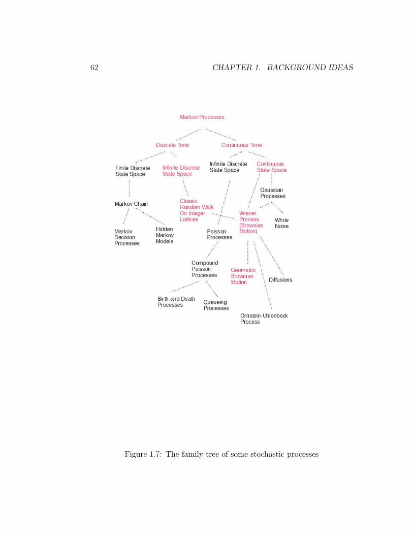
62 CHAPTER 1. BACKGROUND IDEAS
Figure 1.7: The family tree of some stochastic processes

1.7. STOCHASTIC PROCESSES 63
of elementary probability theory. In elementary probability theory, randomvariables are a mapping from a sample space to the real numbers, for stochas-tic processes the mapping is from a sample space to a space of functions. Nowwe can ask questions like
• “What is the probability of the set of functions that exceed a fixedvalue on a fixed time interval?”
• “What is the probability of the set of functions having a certain limitat infinity?”
• “What is the probability of the set of functions which are differentiableeverywhere?”
This is a fruitful way to consider stochastic processes, but it requires sophis-ticated mathematical tools and careful analysis.
Another way to look at stochastic processes is to ask what happens atspecial times. For example, one can consider the time it takes until thefunction takes on one of two certain values, say a and b to be specific. Thenone can ask “What is the probability that the stochastic process assumesthe value a before it assumes the value b?” Note that here the time thateach function assumes the value a is different, it becomes a random time.This provides an interaction between the time variable and the sample pointthrough the values of the function. This too is a fruitful way to think aboutstochastic processes.
In this text, we will consider each of these approaches with the corre-sponding questions.
Sources
The material in this section is adapted from many texts on probability theoryand stochastic processes, especially the classic texts by S. Karlin and H.Taylor, S. Ross, and W. Feller.
Problems to Work for Understanding
Outside Readings and Links:
1. Origlio, Vincenzo. “Stochastic.” From MathWorld–A Wolfram WebResource, created by Eric W. Weisstein. Stochastic
64 CHAPTER 1. BACKGROUND IDEAS
2. Weisstein, Eric W. “Stochastic Process.” From MathWorld–A WolframWeb Resource. Stochastic Process
3. Weisstein, Eric W. “Markov Chain.” From MathWorld–A WolframWeb Resource. Markov Chain
4. Weisstein, Eric W. “Markov Process.” From MathWorld–A WolframWeb Resource. Markov Process
5. Julia Ruscher studying stochastic processes
1.8 A Binomial Model of Mortgage Collater-
alized Debt Obligations (CDOs)
Rating
Mathematically Mature: may contain mathematics beyond calculus withproofs.
Section Starter Question
How do you evaluate cumulative binomial probabilities when the value of nis large, and the value of p is small?
Key Concepts
1. We can make a simple mathematical model of a financial derivativeusing only the idea of a binomial probability.
2. We must investigate the sensitivity of the model to the parameter valuesin order to completely understand the model.
3. This simple model provides our first illustration of the model cycleapplied to a situation in mathematical finance, but even so, it yieldsvaluable insights.

1.8. A BINOMIAL MODEL OF MORTGAGE COLLATERALIZED DEBT OBLIGATIONS (CDOS)65
Vocabulary
1. A tranche is a portion or slice of a set of other securities. The commonuse of tranche is an issue of bonds, often derived from mortgages, thatis distinguished from other tranches by maturity or rate of return.
2. A collateralized debt obligation or CDO is a derivative securitybacked by a pool or slice of other securities. CDOs can be made upof any type of debt and do not necessarily derive from mortgages. Se-curities or bonds derived from mortgages are more specifically calledCollateralized Mortgage Obligations or CMOs or even more specificallyRMBS for “residential mortgage backed securities”. The terms are of-ten used interchangeably but CDO is the most common. CDOs aredivided into slices, each slice is made up of debt which has a uniqueamount of risk associated with it. CDOs are often sold to investorswho want exposure to the income generated by the debt but do notwant to purchase the debt itself.
Mathematical Ideas
A binomial model of mortgages
We will make a simple binomial probability model of a financial instrumentcalled a CDO, standing for “Collateralized Debt Obligation”. The marketin this derivative financial instrument is large, amounting to at least $1.3trillion dollars, of which 56% comes from derivatives based on residentialmortgages. Heavy reliance on these financial derivatives based on the realestate market contributed to the demise of some old-line brokerage firms suchas Bear Stearns and Merrill Lynch in the autumn of 2008. The quick lossin value of these derivatives sparked a lack of economic confidence whichled to the sharp economic downturn in the fall of 2008 and the subsequentrecession. We will build a simple model of these instruments, and even thissimple model will demonstrate that the CDOs were far more sensitive tomortgage failure rates than was commonly understood. While this modelis not sufficient to fully describe CDOs, it does provide an interesting andaccessible example of the modeling process in mathematical finance.
Consider the following financial situation. A loan company has made 100mortgage loans to home-buyers. We will assume
66 CHAPTER 1. BACKGROUND IDEAS
• For simplicity, each loan will have precisely one of 2 outcomes. Eitherthe home-buyer will pay off the loan resulting in a profit of 1 unitof money to the lender, or the home-buyer will default on the loan,resulting in a payoff or profit to the company of 0. For further simplicitywe will say that the unit profit is $1. (The payoff is typically in thethousands of dollars.)
• We will assume that the probability of default on a loan is p and wewill assume that the probability of default on each loan is independentof default on all the other loans.
Let S100 be the number of loans that default, resulting in a total profitof 100 − S100. The probability of n or fewer of these 100 mortgage loansdefaulting is
P [S100 ≤ n] =100∑j=0
(100
j
)(1− p)100−jpj.
We can evaluate this expression in several ways including direct calculationand approximation methods. For our purposes here, one can use a binomialprobability table, or more easily a computer program which has a cumulativebinomial probability function. The expected number of defaults is 100p, theresulting expected loss is 100p and the expected profit is 100(1− p).
But instead of simply making the loans and waiting for them to be paid offthe loan company wishes to bundle these debt obligations differently and sellthem as a financial derivative contract to an investor. Specifically, the loancompany will create a collection of 100 contracts called tranches. Tranche 1will pay 1 dollar if 0 of the loans default. Tranche 2 will pay 1 dollar if 1 of theloans defaults, and in general tranche n will pay 1 dollar if n− 1 or fewer ofthe loans defaults. (This construction is a much simplified model of mortgagebacked securities. In actual practice mortgages with various levels of risk arecombined and then sliced with differing levels of risk into derivative securitiescalled tranches. A tranche is usually backed by thousands of mortgages.)
Suppose to be explicit that 5 of the 100 loans defaults. Then the sellerwill have to pay off tranches 6 through 101. The lender who creates thetranches will receive 95 dollars from the 95 loans which do not default andwill pay out 95. If the lender prices the tranches appropriately, then thelender will have enough money to cover the payout and will have some profitin addition.
1.8. A BINOMIAL MODEL OF MORTGAGE COLLATERALIZED DEBT OBLIGATIONS (CDOS)67
Now from the point of view of the contract buyer, the tranche will eitherpay off with a value of 1 or will default. The probability of payoff on tranchei will be the sum of the probabilities that i− 1 or fewer mortgages default:
i−1∑j=0
(100
j
)pj(1− p)100−j,
that is, a binomial cumulative distribution function. The probability of de-fault on tranche i will be a binomial complementary distribution function,which we will denote by
pT (i) = 1−i−1∑j=0
(100
j
)pj(1− p)100−j.
We should calculate a few default probabilities: The probability of defaulton tranche 1 is the probability of 0 defaults among the 100 loans,
pT (1) = 1−(
100
0
)p0(1− p)100 = 1− (1− p)100.
If p = 0.05, then the probability of default is 0.99408. But for the tranche10, the probability of default is 0.028188. By the 10th tranche, this financialconstruct has created an instrument that is safer than owning one of theoriginal mortgages! Note that because the newly derived security combinesthe risks of several individual loans, under the assumptions of the model itis less exposed to the potential problems of any one borrower.
The expected payout from the collection of tranches will be
E [U ] =100∑n=0
n∑j=0
(100
j
)pj(1− p)100−j =
100∑j=0
j
(100
j
)pj(1− p)100−j = 100p.
That is, the expected payout from the collection of tranches is exactly thesame the expected payout from the original collection of mortgages. However,the lender will also receive the excess value or profit of the tranches sold.Moreover, since the lender is now only selling the possibility of a payoutderived from mortgages and not the mortgages themselves, the lender cansell the same tranche several times to several different buyers.
Why rebundle and sell mortgages as tranches? The reason is that formany of the tranches the risk exposure is less, but the payout is the same

68 CHAPTER 1. BACKGROUND IDEAS
as owning a mortgage loan. Reduction of risk with the same payout is verydesirable for many investors. Those investors may even pay a premium forlow risk investments. In fact, some investors like pension funds are requiredby law, regulation or charter to invest in securities that have a low risk. Someinvestors may not have direct access to the mortgage market, again by law,regulation or charter, but in a rising (or bubble) market they desire to getinto that market. These derivative instruments look like a good investmentto them.
Collateralized Debt Obligations
If rebundling mortgages once is good, then doing it again should be better! Sonow assume that the loan company has 10,000 loans, and that it divides theseinto 100 groups of 100 each, and creates tranches. Now the lender gathersup the 100 10-tranches from each group into a secondary group and bundlesthem just as before, paying off 1 unit if i − 1 or fewer of these 10-tranchesdefaults. These new derivative contracts are now called collateralized debtobligations or CDOs. Again, this is a much simplified model of a realCDO, see [26]. Sometimes, these second level constructs are called a “CDOsquared” [18]. Just as before, the probability of payout for the CDO i iseasily seen to be
i−1∑j=0
(100
j
)pT (i)j(1− pT (i))100−j
and the probability of default is
pCDO(i) = 1−i−1∑j=0
(100
j
)pT (i)j(1− pT (i))100−j.
For example, pCDO(10) = 0.00054385. Roughly, the CDO has only 1/100 ofthe default probability of the original mortgages, by virtue of re-distributingthe risk.
Sensitivity to the parameters
Now we investigate the robustness of the model. We do this by varying theprobability of mortgage default to see how it affects the risk of the tranchesand the CDOs.
1.8. A BINOMIAL MODEL OF MORTGAGE COLLATERALIZED DEBT OBLIGATIONS (CDOS)69
Assume that the underlying mortgages actually have a default probabilityof 6%, a 20% increase in the risk although it is only a 1% increase in the actualrates. This change in the default rate may be due to several factors. Onemay be the inherent inability to measure a fairly subjective parameter such as“mortgage default rate” accurately. Finding the probability of a home-ownerdefaulting is not the same as calculating a losing bet in a dice game. Anothermay be a faulty evaluation (usually over confident or optimistic) of the defaultrates themselves by the agencies who provide the service of evaluating therisk on these kinds of instruments. Some economic commentators allegethat before the 2008 economic crisis the rating agencies were under intensecompetitive pressure to provide “good” ratings in order to get the businessof the firms who create derivative instruments and may have shaded theirratings to the favorable side in order to keep the business. Finally, theunderlying economic climate may be changing and the previous estimate,while reasonable for the prior conditions, is no longer valid. If the economydeteriorates or the jobless rate increases, weak mortgages called sub-primemortgages may default at increased rates.
Now we calculate that the 10-tranches have a default probability of 7.8%,a 275% increase from the previous rate of 2.8%. Worse, the 10th CDO madeof 10-Tranches will have a default probability of 24.7%, an increase of over45,400%! The financial derivatives amplify any error in measuring the defaultrate to a completely unacceptable risk. The model shows that the financialinstruments are not robust to errors in the assumptions!
But shouldn’t the companies either buying or selling the derivatives recog-nize this? There is a human tendency to blame failures, including the failuresof the Wall Street giants, on ignorance, incompetence or wrongful behavior.In this case, the traders and “rocket scientists” who created the CDOs wereprobably neither ignorant nor incompetent. Because they ruined a profitableendeavor for themselves, we can probably rule out malfeasance too. But dis-traction resulting from an intense competitive environment allowing no timefor rational reflection along with overconfidence during a bubble can makeus willfully ignorant of the conditions. A failure to properly complete themodeling cycle leads the users to ignore the very real risks.
Criticism of the model
This model is far too simple to base any investment strategy or more seriouseconomic analysis on it. First, an outcome of either pay-off or default is too
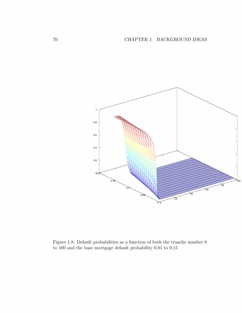
70 CHAPTER 1. BACKGROUND IDEAS
Figure 1.8: Default probabilities as a function of both the tranche number 0to 100 and the base mortgage default probability 0.01 to 0.15

1.8. A BINOMIAL MODEL OF MORTGAGE COLLATERALIZED DEBT OBLIGATIONS (CDOS)71
simple. Lenders will restructure shaky loans or they will sell them to otherfinancial institutions so that the lenders will get some return, even if lessthan originally intended.
The assumption of a uniform probability of default is too simple by far.Lenders make some loans to safe and reliable home-owners who dutifully payoff the mortgage in good order. Lenders also make some questionable loans topeople with poor credit ratings, these are called sub-prime loans or sub-primemortgages. The probability of default is not the same. In fact, mortgagesand loans are graded according to risk. There are 20 grades ranging fromAAA with a 1-year default probability of less than 0.1% through BBB with a1-year default probability of slightly less than 1% to CC with a 1-year defaultprobability of more than 35%. The mortgages may also change their ratingover time as economic conditions change, and that will affect the derivedsecurities. Also too simple is the assumption of an equal unit payoff for eachloan, but this is a less serious objection.
The assumption of independence is clearly incorrect. The similarity of themortgages increases the likelihood that they will all prosper or suffer togetherand potentially default at once. Due to external economic conditions, suchas an increase in the unemployment rate or a downturn in the economy,default on one loan may indicate greater probability of default on other,even geographically separate loans, especially sub-prime loans. This is themost serious objection to the model, since it invalidates the use of binomialprobabilities.
However, relaxing any assumptions make the calculations much more diffi-cult. The non-uniform probabilities and the lack of independence means thatelementary theoretical tools from probability are not sufficient to analyze themodel. Instead, simulation models will be the next means of analysis.
Nevertheless, the sensitivity of the simple model should make us verywary of optimistic claims about the more complicated model.
Sources
This section is adapted from a presentation by Jonathan Kaplan of D.E.Shaw and Co. in summer 2010. The definitions are derived from definitionsat investorwords.com. The definition of CDO squared is noted in [18, page166]. Some facts and figures are derived from the graphics at Portfolio.com:What’s a CDO [40] and Wall Street Journal.com : The Making of a MortgageCDO, [26]
72 CHAPTER 1. BACKGROUND IDEAS
Problems to Work for Understanding
1. Suppose that there is a 20% decrease in the default rate from 5% to4%. By what factor do the default rates of the 10-tranches and thederived 10th CDO change?
2. For the tranches create a table of probabilities of default for tranchesi = 5 to i = 15 for probabilities of default p = 0.03, 0.04, 0.05 0.06 and0.07 and determine where the tranches become safer investments thanthe individual mortgages on which they are based.
3. For a base mortgage default rate of 5%, draw the graph of the defaultrate of the tranches as a function of the tranche number.
4. The text asserts that the expected payout from the collection of trancheswill be
E [U ] =100∑n=0
n∑j=0
(100
j
)pj(1−p)100−j =
100∑j=0
j
(100
j
)pj(1−p)100−j = 100p.
That is, the expected payout from the collection of tranches is exactlythe same the expected payout from the original collection of mortgages.More generally, show that
N∑n=0
n∑j=0
aj =N∑j=0
j · aj.
Outside Readings and Links:
1. Wall Street Journal.com : The Making of a Mortgage CDO An an-imated graphic explanation from the Wall Street Journal describingmortgage backed debt obligations.
2. Portfolio.com: What’s a CDO Another animated graphic explanationfrom Portfolio.com describing mortgage backed debt obligations.

Chapter 2
Binomial Option PricingModels
2.1 Single Period Binomial Models
Rating
Student: contains scenes of mild algebra or calculus that may require guid-ance.
Section Starter Question
Two items can be purchased in any amounts each, call the amounts x andy. (Think about stocks and bonds.) The two items each contribute revenueat rates specific to the current financial environment. (Think about stockprofits in good times and bad, call them rgx and rbx and bond interest atrates rgy and rby.) Two specific outcomes must be achieved, one in goodtimes, one in bad times (call them fg and fb). What mathematical set-up isrequired to find the specific amounts of each item?
Key Concepts
1. The simplest model for pricing an option is based on a market havinga single period, a single security having two uncertain outcomes, and asingle bond.
73

74 CHAPTER 2. BINOMIAL OPTION PRICING MODELS
2. Replication of the option payouts with the single security and the singlebond leads to pricing the derivative by arbitrage.
Vocabulary
1. Security: A promise to pay, or an evidence of a debt or property,typically a stock or a bond. Also referred to as an asset.
2. Bond: Interest bearing securities, which can either make regular in-terest payments, or a lump sum payment at maturity, or both.
3. Stock: A security representing partial ownership of a company, varyingin value with the value of the company. Also known as shares orequities.
4. Derivative: A security whose value depends on or is derived fromthe future price or performance of another security. Also known asfinancial derivatives, derivative securities, derivative products,and contingent claims.
5. A portfolio of the stock and the bond which will have the same valueas the derivative itself in any circumstance is a replicating portfolio.
Mathematical Ideas
Single Period Binomial Model
The single period binomial model is the simplest possible financial model,yet it contains the elements of all future models. The single period binomialmodel is an excellent place to start studying mathematical finance. It isstrong enough to be a somewhat realistic model of financial markets. It issimple enough to permit pencil-and-paper calculation. It can be compre-hended as a whole. It is also structured enough to point to natural general-ization.
The quantifiable elements of the single period binomial financial modelare:
1. A single interval of time, from t = 0 to t = T .

2.1. SINGLE PERIOD BINOMIAL MODELS 75
2. A single stock of initial value S, in the time interval [0, T ] it can eitherincrease by a factor U to value SU with probability p, or it can decreasein value by factor D to value SD with probability q = 1− p.
3. A single bond with a continuously compounded interest rate r over theinterval [0, T ]. If the initial value of the bond is B, then the final valueof the bond will be B exp(rT ).
4. A market for derivatives (such as options) dependent on the value ofthe stock at the end of the period. The payoff of the derivative tosome investor would be the rewards (or penalties) f(SU) and f(SD).For example, a futures contract with strike price K would have valuef(ST ) = ST −K. A call option with strike price K, would have valuef(ST ) = max(ST −K, 0).
A realistic financial assumption would be that D < exp(rT ) < U . Theninvestment in the risky security may pay better than investment in a risk freebond, but it may also pay less! The mathematics only requires that U 6= D,see below.
We can attempt to find the value of the derivative by creating a portfolioof the stock and the bond which will have the same value as the derivativeitself in any circumstance, called a replicating portfolio. Consider a port-folio consisting of φ units of the stock worth φS and ψ units of the bondworth ψB. (Note we are making the assumption that the stock and bondare divisible, we can buy them in any amounts including negative amountswhich are short positions.) If we were to buy the this portfolio at time zero,it would cost
φS + ψB.
One time period of length T on the trading clock later, the portfolio wouldbe worth
φSD + ψB exp(rT )
after a down move and
φSU + ψB exp(rT )
after an up move. You should find this mathematically meaningful: thereare two unknown quantities φ and ψ to buy for the portfolio, and we havetwo expressions to match with the two values of the derivative! That is, the

76 CHAPTER 2. BINOMIAL OPTION PRICING MODELS
Figure 2.1: The single period binomial model.

2.1. SINGLE PERIOD BINOMIAL MODELS 77
portfolio will have the same value as the derivative if
φSD + ψB exp(rT ) = f(SD)
φSU + ψB exp(rT ) = f(SU)
The solution is
φ =f(SU)− f(SD)
SU − SDand
ψ =f(SD)
B exp(rT )− (f(SU)− f(SD))SD
(SU − SD)B exp(rT ).
Note that the solution requires SU 6= SD, but we have already assumed thisnatural requirement. Without this requirement there would be no risk in thestock, and we would not be asking the question in the first place! The value(or price) of the portfolio, and therefore the derivative should then be
V = φS + ψB
= Sf(SU)− f(SD)
SU − SD+B[
f(SD)
B exp(rT )− (f(SU)− f(SD))SD
(SU − SD)B exp(rT )].
=f(SU)− f(SD)
U −D+
1
exp(rT )
f(SD)U − f(SU)D
(U −D).
We can make one final simplification that will be useful in the next section.Define
π =exp(rT )−D
U −Dso then
1− π =U − exp(rT )
U −Dso that we write the value of the derivative as
exp(−rT )[πf(SU) + (1− π)f(SD)].
(Here π is not used as the mathematical constant giving the ratio of thecircumference of a circle to its diameter. Instead the Greek letter for psuggests a similarity to the probability p.)
Now consider some other trader offering to sell this derivative with payofffunction f for a price P less than V . Anyone could buy the derivative inarbitrary quantity, and short the (φ, ψ) stock-bond portfolio in exactly the

78 CHAPTER 2. BINOMIAL OPTION PRICING MODELS
same quantity. At the end of the period, the value of the derivative would beexactly the same as the portfolio. So selling each derivative would repay theshort with a profit of V − P and the trade carries no risk! So P would nothave been a rational price for the trader to quote and the market would havequickly mobilized to take advantage of the “free” money on offer in arbitraryquantity. (This ignores transaction costs. For an individual, transactioncosts might eliminate the profit. However for large firms trading in largequantities, transaction costs can be minimal.)
Similarly if a seller quoted the derivative at a price P greater than V ,anyone could short sell the derivative and buy the (φ, ψ) portfolio to lockin a risk-free profit of P − V per unit trade. Again the market would takeadvantage of the opportunity. Hence, V is the only rational price for thederivative. We have determined the price of the derivative through arbitrage.
How NOT to price the derivative and a hint of a better way.
Note that we did not determine the price of the derivative in terms of theexpected value of the stock or the derivative. A seemingly logical thing to dowould be to say that the derivative will have value f(SU) with probabilityp and will have value f(SD) with probability 1− p. Therefore the expectedvalue of the derivative at time T is
E [f ] = pf(SU) + (1− p)f(SD).
The present value of the expectation of the derivative value is
exp(−rT )E [f ] = exp(−rT )[pf(SU) + (1− p)f(SD)].
Except in the peculiar case that the expected value just happened to matchthe value V of the replicating portfolio, pricing by expectation would bedriven out of the market by arbitrage! The problem is that the probabilitydistribution (p, 1− p) only takes into account the movements of the securityprice. The expected value is the value of the derivative over many identicaliterations or replications of that distribution, but there will be only one trialof this particular experiment, so expected value is not a reasonable way toweight the outcomes. Also, the expected value does not take into accountthe rest of the market. In particular, the expected value does not take intoaccount that an investor has the opportunity to simultaneously invest inalternate combinations of the risky stock and the risk-free bond. A special

2.1. SINGLE PERIOD BINOMIAL MODELS 79
combination of the risky stock and risk-free bond replicates the derivative.As such the movement probabilities alone do not completely assess the riskassociated with the transaction.
Nevertheless, we are left with a nagging feeling that pricing by arbitrageas done above ignores the probability associated with security price changes.One could legitimately ask if there is a way to value derivatives by takingsome kind of expected value. The answer is yes, there is another probabilitydistribution associated with the binomial model that correctly takes intoaccount the rest of the market. In fact, the quantities π and 1−π define thisprobability distribution. This is called the risk-neutral measure or morecompletely the risk-neutral martingale measure and we will talk moreabout it later. Economically speaking, the market assigns a “fairer” set ofprobabilities π and 1−π that give a value for the option compatible with theno arbitrage principle. Another way to say this is that the market changesthe odds to make option pricing fairer. The risk-neutral measure approachis the very modern, sophisticated, and general way to approach derivativepricing. However it is too advanced for us to approach just yet.
Summary
From R. C. Merton in “Influence of mathematical models in finance on prac-tice: past, present and future”, in Mathematical Models in Finance, editedby S.D. Howison, F. P. Kelly, and P. Wilmott, Chapman and Hall, London,1995, pages 1-15.
“The basic insight underlying the Black-Scholes model is thata dynamic portfolio trading strategy in the stock can be foundwhich will replicate the returns from an option on that stock.Hence, to avoid arbitrage opportunities, the option price mustalways equal the value of this replicating portfolio.”
Sources
This section is adapted from: “Chapter 2, Discrete Processes” in FinancialCalculus by M. Baxter, A. Rennie, Cambridge University Press, Cambridge,1996, [5].
80 CHAPTER 2. BINOMIAL OPTION PRICING MODELS
Problems to Work for Understanding
1. Consider a stock whose price today is $50. Suppose that over the nextyear, the stock price can either go up by 10%, or down by 3%, so thestock price at the end of the year is either $55 or $48.50. The interestrate on a $1 bond is 6%. If there also exists a call on the stock with anexercise price of $50, then what is the price of the call option? Also,what is the replicating portfolio?
2. A stock price is currently $50. It is known that at the end of 6 months,it will either be $60 or $42. The risk-free rate of interest with continuouscompounding on a $1 bond is 12% per annum. Calculate the value ofa 6-month European call option on the stock with strike price $48 andfind the replicating portfolio.
3. A stock price is currently $40. It is known that at the end of 3 months,it will either $45 or $34. The risk-free rate of interest with quarterlycompounding on a $1 bond is 8% per annum. Calculate the value of a3-month European put option on the stock with a strike price of $40,and find the replicating portfolio.
4. Your friend, the financial analyst comes to you, the mathematicaleconomist, with a proposal: “The single period binomial pricing is allright as far as it goes, but it is certainly is simplistic. Why not modifyit slightly to make it a little more realistic? Specifically, assume thestock can assume three values at time T , say it goes up by a factorU with probability pU , it goes down by a factor D with probabilitypD, where D < 1 < U and the stock stays somewhere in between,changing by a factor M with probability pM where D < M < U andpD + pM + pU = 1.” The market contains only this stock, a bondwith a continuously compounded risk-free rate r and an option on thestock with payoff function f(ST ). Make a mathematical model basedon your friend’s suggestion and provide a critique of the model basedon the classical applied mathematics criteria of existence of solutionsto the model and uniqueness of solutions to the model.
Outside Readings and Links:
1. A video lesson on the binomial option model from Hull

2.2. MULTIPERIOD BINOMIAL TREE MODELS 81
2.2 Multiperiod Binomial Tree Models
Rating
Student: contains scenes of mild algebra or calculus that may require guid-ance.
Section Starter Question
Suppose that you owned a 3-month option, and that you tracked the value ofthe underlying security at the end of each month. Suppose you were forcedto sell the option at the end of two months. How would you determine a fairprice for the option at that time? What simple modeling assumptions wouldyou make?
Key Concepts
1. A multiperiod binomial derivative model can be valued by dynamicprogramming — computing the replicating portfolio and correspondingportfolio values back one period at a time from the claim values to thestarting time.
Vocabulary
1. The multiperiod binomial model for pricing derivatives of a risky secu-rity is also called the Cox-Ross-Rubenstein model or CRR modelfor short, after those who introduced it in 1979.
Mathematical Ideas
The Binomial Tree model
The multiperiod binomial model has N time intervals created by N + 1trading times t0 = 0, t1, . . . , tN = T . The spacing between time intervalsis ∆ti = ti − ti−1, and typically the spacing is equal, although it is notnecessary. The time intervals can be any convenient time length appropriatefor the model, e.g. months, days, minutes, even seconds. Later, we will takethem to be relatively short compared to T .
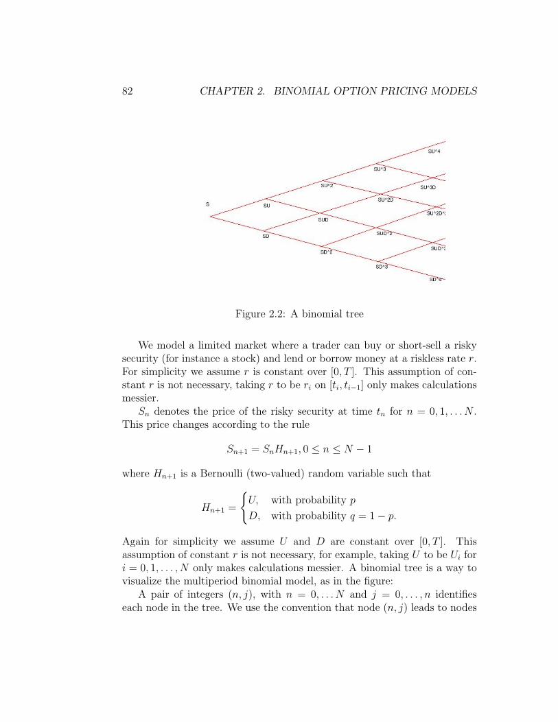
82 CHAPTER 2. BINOMIAL OPTION PRICING MODELS
Figure 2.2: A binomial tree
We model a limited market where a trader can buy or short-sell a riskysecurity (for instance a stock) and lend or borrow money at a riskless rate r.For simplicity we assume r is constant over [0, T ]. This assumption of con-stant r is not necessary, taking r to be ri on [ti, ti−1] only makes calculationsmessier.
Sn denotes the price of the risky security at time tn for n = 0, 1, . . . N .This price changes according to the rule
Sn+1 = SnHn+1, 0 ≤ n ≤ N − 1
where Hn+1 is a Bernoulli (two-valued) random variable such that
Hn+1 =
U, with probability p
D, with probability q = 1− p.
Again for simplicity we assume U and D are constant over [0, T ]. Thisassumption of constant r is not necessary, for example, taking U to be Ui fori = 0, 1, . . . , N only makes calculations messier. A binomial tree is a way tovisualize the multiperiod binomial model, as in the figure:
A pair of integers (n, j), with n = 0, . . . N and j = 0, . . . , n identifieseach node in the tree. We use the convention that node (n, j) leads to nodes

2.2. MULTIPERIOD BINOMIAL TREE MODELS 83
(n + 1, j) and (n + 1, j + 1) at the next trading time, with the “up” changecorresponding to (n + 1, j + 1) and the “down” change corresponding to(n + 1, j). The index j counts the number of up changes to that time, son − j is the number of down changes. Several paths lead to node (n, j), infact
(nj
)of them. The price of the risky underlying asset at trading time tn
is then SU jDn−j. The probability of going from price S to price SU jDn−j is
pn,j =
(n
j
)pj(1− p)n−j.
To value a derivative with payout f(SN), the key idea is that of dynamicprogramming — extending the replicating portfolio and corresponding port-folio values back one period at a time from the claim values to the startingtime.
An example will make this clear. Consider a binomial tree on the timest0, t1, t2. Assume U = 1.05, D = 0.95, and exp(r∆ti) = 1.02, so the effectiveinterest rate on each time interval is 2%. We take S0 = 100. We value aEuropean call option with strike price K = 100. Using the formula derivedin the previous section
π =1.02− 0.95
1.05− 0.95= 0.7
and 1−π = 0.3. Then concentrating on the single period binomial branch inthe large square box, the value of the option at node (1, 1) is $7.03. Likewise,the value of the option at node (1, 0) is $0. Then we work back one step andvalue a derivative with potential payouts $7.03 and $0 on the single periodbinomial branch at (0, 0). This uses the same arithmetic to obtain the value$4.82 at time 0. In the figure, the values of the security at each node are inthe circles, the value of the option at each node is in the small box besidethe circle.
As another example, consider a European put on the same security. Thestrike price is again 100. All of the other parameters are the same. We workbackward again through the tree to obtain the value at time 0 as $0.944. Inthe figure, the values of the security at each node are in the circles, the valueof the option at each node is in the small box beside the circle.
The multiperiod binomial model for pricing derivatives of a risky securityis also called the Cox-Ross-Rubenstein model or CRR model for short,after those who introduced it in 1979.

84 CHAPTER 2. BINOMIAL OPTION PRICING MODELS
Figure 2.3: Pricing a European call
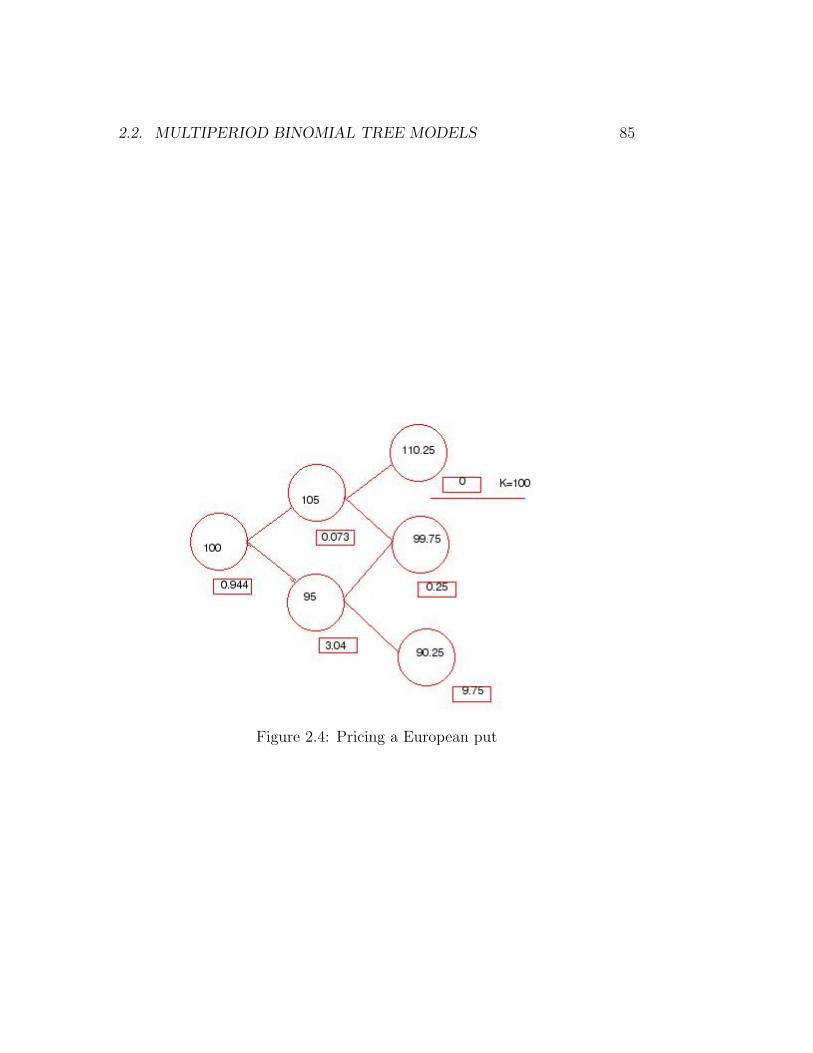
2.2. MULTIPERIOD BINOMIAL TREE MODELS 85
Figure 2.4: Pricing a European put

86 CHAPTER 2. BINOMIAL OPTION PRICING MODELS
Advantages and Disadvantages of the model
The disadvantages of the binomial model are:
1. Trading times are not really at discrete times, trading goes on contin-uously.
2. Securities do not change value according to a Bernoulli (two-valued)distribution on a single time step, or a binomial distribution on multipletime periods, they change over a range of values with a continuousdistribution.
3. The calculations are tedious.
4. Developing a more complete theory is going to take some detailed andserious limit-taking considerations.
The advantages of the model are:
1. It clearly reveals the construction of the replicating portfolio.
2. It clearly reveals that the probability distribution is not centrally in-volved, since expectations of outcomes aren’t used to value the deriva-tives.
3. It is simple to calculate, although it can get tedious.
4. It reveals that we need more probability theory to get a complete un-derstanding of path dependent probabilities of security prices.
It is possible, with considerable attention to detail, to make a limitingargument and pass from the binomial tree model of Cox, Ross and Rubensteinto the Black-Scholes pricing formula. However, this approach is not the mostinstructive. Instead, we will back up from derivative pricing models, andconsider simpler models with only risk, that is, gambling, to get a morecomplete understanding before returning to pricing derivatives.
Some caution is also needed when reading from other sources about theCox-Ross-Rubenstein or Binomial Option Pricing Model. Many other sourcesderive the Binomial Option Pricing Model by discretizing the Black-ScholesOption Pricing Model. The discretization is different from building the model
2.2. MULTIPERIOD BINOMIAL TREE MODELS 87
from scratch because the parameters have special and more restricted inter-pretations than the simple model. More sophisticated discretization proce-dures from the numerical analysis of partial differential equations also lead toadditional discrete option pricing models which are hard to justify by build-ing them from scratch. The discrete models derived from the Black-Scholesmodel are used for simple and rapid numerical evaluation of option pricesrather than motivation.
Sources
This section is adapted from: “Chapter 2, Discrete Processes” in FinancialCalculus by M. Baxter, A. Rennie [5] and Quantitative Modeling of DerivativeSecurities by M. Avellaneda and P. Laurence [2].
Problems to Work for Understanding
1. Consider a two-time-stage example. Each time stage is a year. A stockstarts at 50. In each year, the stock can go up by 10% or down by 3%.The continuously compounded interest rate on a $1 bond is constantat 6% each year. Find the price of a call option with exercise price50, with exercise date at the end of the second year. Also, find thereplicating portfolio at each node.
2. Consider a three-time-stage example. The first time interval is a month,then the second time interval is two months, finally, the third timeinterval is a month again. A stock starts at 50. In the first interval, thestock can go up by 10% or down by 3%, in the second interval the stockcan go up by 5% or down by 5%, finally in the third time interval, thestock can go up by 6% or down by 3%. The continuously compoundedinterest rate on a $1 bond is 2% in the fist period, 3% in the secondperiod, and 4% in the third period. Find the price of a call option withexercise price 50, with exercise date at the end of the 4 months. Also,find the replicating portfolio at each node.
3. A European cash-or-nothing binary option pays a fixed amount ofmoney if it expires with the underlying stock value above the strikeprice. The binary option pays nothing if it expires with the underlyingstock value equal to or less than the strike price. A stock currently hasprice $100 and goes up or down by 20% in each time period. What is
88 CHAPTER 2. BINOMIAL OPTION PRICING MODELS
the value of such a cash-or-nothing binary option with payoff $100 atexpiration 2 time units in the future and strike price $100? Assume asimple interest rate of 10% in each time period.
4. A long strangle option pays max(K1 − S, 0, S −K2) if it expires whenthe underlying stock value is S. The parameters K1 and K2 are thelower strike price and the upper strike price, and K1 < K2. A stockcurrently has price $100 and goes up or down by 20% in each timeperiod. What is the value of such a long strangle option with lowerstrike 90 and upper strike 110 at expiration 2 time units in the future?Assume a simple interest rate of 10% in each time period.
5. A long straddle option pays |S −K| if it expires when the underlyingstock value is S. The option is a portfolio composed of a call and aput on the same security with K as the strike price for both. A stockcurrently has price $100 and goes up or down by 10% in each timeperiod. What is the value of such a long straddle option with strikeprice K = 110 at expiration 2 time units in the future? Assume asimple interest rate of 5% in each time period.
Outside Readings and Links:
1. Peter Hoadley, Options Strategy Analysis Tools. A useful link on ba-sics of the Black Scholes option pricing model. It contains terminology,calculator, animated graphs, and Excel addins (a free trial version) formaking a spreadsheet model. Submitted by Yogesh Makkar, September9,2003.
2. Binomial Tree Option Pricing by Simon Shaw, Brunel University Theweb page contains an applet that implements the Binomial Tree OptionPricing technique, and gives a short outline of the mathematical theorybehind the method. Submitted by Chun Fan, September 10, 2003.
Chapter 3
First Step Analysis forStochastic Processes
3.1 A Coin Tossing Experiment
Rating
Everyone: contains no mathematics.
Section Starter Question
Suppose you start with a fortune of $10, and you want to gamble to have$20 before you go broke. You flip a fair coin successively, and gain $1 if thecoin comes up “Heads” and loses $1 if the coin comes up “Tails”. What doyou estimate is the probability of getting to $20 before going broke? Howlong do you estimate it take before one of the two outcomes occurs? How doestimate each?
Key Concepts
1. Performing an experiment to gain intuition and experience with coin-tossing games.
Vocabulary
1. We call victory the state of reaching a fortune goal, before going broke.
89
90CHAPTER 3. FIRST STEP ANALYSIS FOR STOCHASTIC PROCESSES
2. We call ruin the state of going broke before reaching a fortune goal.
Mathematical Ideas
Reasons for Modeling with a Coin Flipping Game
We need a better understanding of the paths that risky securities take. Weshall make and investigate a greatly simplified model. For our model, weassume:
1. Time is discrete, occurring at t0 = 0, t1, t2, . . ..
2. There are no risk-free investments available, (i.e. no bonds on the mar-ket).
3. There are no options, and no financial derivatives.
4. The only investments are risk-only, that is, our fortune at any time isa random variable:
Tn+1 = Tn + Yn+1
where T0 is our given initial fortune, and for simplicity,
Yn =
+1 probability 1/2
−1 probability 1/2
Our model is commonly called “gambling” and we will investigate the prob-abilities of making a fortune by gambling.
Some Humor
An Experiment
1. Each person should have a chart for recording the outcomes of eachgame (see below) and a sheet of graph paper.
2. Each person should use a fair coin to flip, say a penny.
3. Each “gambler” flips the coin, and records a +1 (gains $1) if the coincomes up “Heads” and records −1 (loses $1) if the coin comes up“Tails”. On the chart, the player records the outcome of each flip

3.1. A COIN TOSSING EXPERIMENT 91
Figure 3.1: Welcome to my casino!
by recording the flip number, the outcome as “H” or “T” and keepstrack of the cumulative fortune of the gambler so far. It is best to keepthese records in a neat chart, since we will refer to them later.
4. Each “gambler” should record 100 flips, which takes about 10 to 20minutes.
Toss n 1 2 3 4 5 6 7 8 9 10H or TYn = +1,−1Tn =
∑ni=1 Yi
Toss n 11 12 13 14 15 16 17 18 19 20H or TYn = +1,−1Tn =
∑ni=1 Yi
Toss n 21 22 23 24 25 26 27 28 29 30H or TYn = +1,−1Tn =
∑ni=1 Yi

92CHAPTER 3. FIRST STEP ANALYSIS FOR STOCHASTIC PROCESSES
Figure 3.2: Welcome to my casino!
Toss n 31 32 33 34 35 36 37 38 39 40H or TYn = +1,−1Tn =
∑ni=1 YI
Toss n 41 42 43 44 45 46 47 48 49 50H or TYn = +1,−1Tn =
∑ni=1 Yi
Toss n 51 52 53 54 55 56 57 58 59 60H or TYn = +1,−1Tn =
∑ni=1 Yi
Toss n 61 62 63 64 65 66 67 68 69 70H or TYn = +1,−1Tn =
∑ni=1 Yi

3.1. A COIN TOSSING EXPERIMENT 93
Toss n 71 72 73 74 75 76 77 78 79 80H or TYn = +1,−1Tn =
∑ni=1 Yi
Toss n 81 82 83 84 85 86 87 88 89 90H or TYn = +1,−1Tn =
∑ni=1 Yi
Toss n 91 92 93 94 95 96 97 98 99 100H or TYn = +1,−1Tn =
∑ni=1 Yi
Some Outcomes
In an in-class experiment with 17 “gamblers”, the class members obtainedthe following results:
1. 8 gamblers reached a net loss of −10 before reaching a net gain of +10,that is, acheived “victory”.
2. 7 gamblers reached a net gain of +10 before reaching a net loss of −10,that is, were “ruined”.
3. 2 gamblers still had not reached a net loss of +10 or −10 yet.
This closely matches the predicted outcomes of 1/2 the gamblers being ru-ined, and 1/2 of the gamblers being victorious.
The durations of the games were 88, 78, 133, 70, 26, 76, 92, 146, 153, 24, 177, 67, 24, 34, 42, 90.The mean duration is 82.5 which is a little short of the predicted expectedduration of 100.
Sources
This section is adapted from ideas in William Feller’s classic text, An Intro-duction to Probability Theory and Its Applications, Volume I, Third Edition.

94CHAPTER 3. FIRST STEP ANALYSIS FOR STOCHASTIC PROCESSES
Problems to Work for Understanding
1. How many heads were obtained in your sequence of 100 flips? Whatis the class average of the number of heads in 100 flips? What is thevariance of the number of heads obtained by the class members in thenumber of heads?
2. How many flips did it take before you reached a net gain of +10 or anet loss of −10? What is the class average of the number of flips beforereaching a net gain of +10 or a net loss of −10?
3. How many of the class reached a net gain of +10 before reaching a netloss of −10?
4. What is the maximum net value achieved in your sequence of flips?What is the class distribution of maximum values achieved in the se-quence of flips?
Outside Readings and Links:
1. Virtual Laboratories in Probability and Statistics Red and Black Game
2. University of California, San Diego, Department of Mathematics, A.M.Garsia A java applet that simulates how long it takes for a gambler togo broke. You can control how much money you and the casino startwith, the house odds, and the maximum number of games. Results area graph and a summary table. Submitted by Matt Odell, September8, 2003.
3.2 Ruin Probabilities
Rating
Mathematically Mature: may contain mathematics beyond calculus withproofs.

3.2. RUIN PROBABILITIES 95
Section Starter Question
What is the solution of the equation xn = axn−1 where a is a constant?What kind of a function is the solution? What more, if anything, needs tobe known to obtain a complete solution?
Key Concepts
1. The probabilities, interpretation, meaning, and consequences of the“gambler’s ruin”.
Vocabulary
1. Classical Ruin Problem “Consider the familiar gambler who winsor loses a dollar with probabilities p and q = 1 − p, respectively play-ing against an infinitely rich adversary who is always willing to playalthough the gambler has the privilege of stopping at his pleasure. Thegambler adopts the strategy of playing until he either loses his capital(“is ruined”) or increases it to a (with a net gain of a − T0.) We areinterested in the probability of the gambler’s ruin and the probabilitydistribution of the duration of the game. This is the classical ruinproblem.”. (From W. Feller, in Introduction to Probability Theory andApplications, Volume I, Chapter XIV, page 342. [15])
Mathematical Ideas
Understanding a Stochastic Process
We consider a sequence of Bernoulli random variables, Y1, Y2, Y3, . . . whereYi = +1 with probability p and Yi = −1 with probability q. We start withan initial value T0. We define the sequence of sums Tn =
∑ni=0 Yi. We
are interested in the stochastic process T1, T2, T3, . . .. It turns out this is acomplicated sequence to understand in full, so we single out particular simplerfeatures to understand first. For example, we can look at the probability thatthe process will achieve the value 0 before it achieves the value a. This isa special case of a larger class of probability problems called first-passageprobabilities.

96CHAPTER 3. FIRST STEP ANALYSIS FOR STOCHASTIC PROCESSES
Theorems about Ruin Probabilities
Consider a gambler who wins or loses a dollar on each turn of a game withprobabilities p and q = 1 − p respectively. Let his initial capital be T0.The game continues until the gambler’s capital either is reduced to 0 or hasincreased to a. Let qT0 be the probability of the gambler’s ultimate ruinand pT0 the probability of his winning. We shall show later that (see alsoDuration of the Game Until Ruin.)
pT0 + qT0 = 1
so that we need not consider the possibility of an unending game.
Theorem 1. The probability of the gambler’s ruin is
qT0 =(q/p)a − (q/p)T0
(q/p)a − 1
if p 6= q and
qT0 = 1− T0/a
if p = q = 1/2.
Proof. After the first trial the gambler’s fortune is either T0−1 or T0 +1 andtherefore we must have
qT0 = pqT0+1 + qqT0−1 (3.1)
provided 1 < T0 < a − 1. For T0 = 1, the first trial may lead to ruin, and(3.1) is replaced by
q1 = pq2 + q.
Similarly, for T0 = a− 1 the first trial may result in victory, and therefore
qa−1 = qqa−2.
To unify our equations, we define as a natural convention that q0 = 1, andqa = 0. Then the probability of ruin satisfies (3.1) for T0 = 1, 2, . . . , a − 1.This defines a set of a− 1 difference equations, with boundary conditions at0 and a. If we solve the system of difference equations, then we will have thedesired probability qT0 for any value of T0.
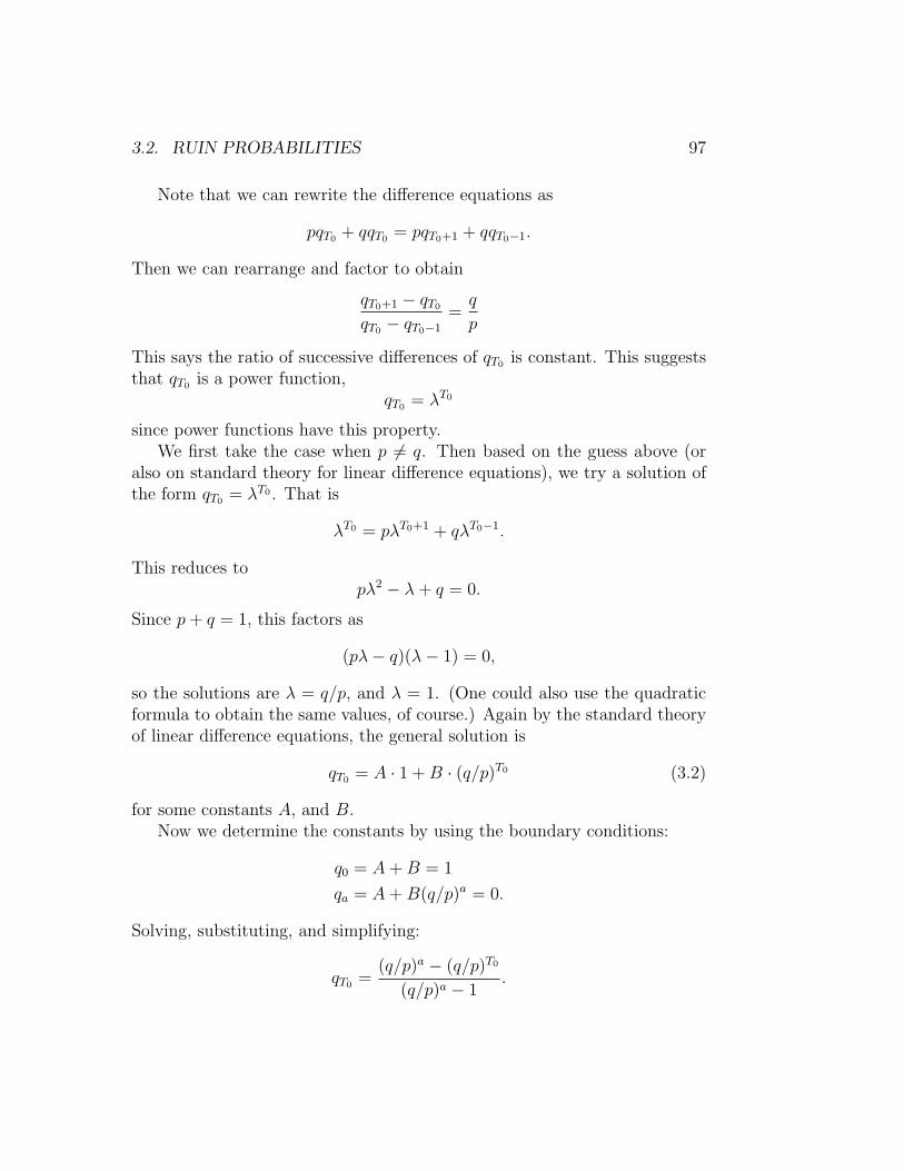
3.2. RUIN PROBABILITIES 97
Note that we can rewrite the difference equations as
pqT0 + qqT0 = pqT0+1 + qqT0−1.
Then we can rearrange and factor to obtain
qT0+1 − qT0
qT0 − qT0−1
=q
p
This says the ratio of successive differences of qT0 is constant. This suggeststhat qT0 is a power function,
qT0 = λT0
since power functions have this property.We first take the case when p 6= q. Then based on the guess above (or
also on standard theory for linear difference equations), we try a solution ofthe form qT0 = λT0 . That is
λT0 = pλT0+1 + qλT0−1.
This reduces topλ2 − λ+ q = 0.
Since p+ q = 1, this factors as
(pλ− q)(λ− 1) = 0,
so the solutions are λ = q/p, and λ = 1. (One could also use the quadraticformula to obtain the same values, of course.) Again by the standard theoryof linear difference equations, the general solution is
qT0 = A · 1 +B · (q/p)T0 (3.2)
for some constants A, and B.Now we determine the constants by using the boundary conditions:
q0 = A+B = 1
qa = A+B(q/p)a = 0.
Solving, substituting, and simplifying:
qT0 =(q/p)a − (q/p)T0
(q/p)a − 1.

98CHAPTER 3. FIRST STEP ANALYSIS FOR STOCHASTIC PROCESSES
(Check for yourself that with this expression 0 ≤ qT0 ≤ 1 as it should be afor a probability.)
We should show that the solution is unique. So suppose rT0 is anothersolution of the difference equations. Given an arbitrary solution of (3.1), thetwo constants A and B can be determined so that (3.2) agrees with rT0 atT0 = 0 and T0 = a. (The reader should be able to explain why by referenceto a theorem in Linear Algebra!) From these two values, all other valuescan be found by substituting in (3.1) successively T0 = 1, 2, 3, . . . Therefore,two solutions which agree for T0 = 0 and T0 = 1 are identical, hence everysolution is of the form (3.2).
The solution breaks down if p = q = 1/2, since then we do not get twolinearly independent solutions of the difference equation (we get the solution1 repeated twice). Instead, we need to borrow a result from differential equa-tions (from the variation-of-parameters/reduction-of-order set of ideas usedto derive a complete linearly independent set of solutions.) Certainly, 1 isstill a solution of the difference equation (3.1). A second linearly independentsolution is T0, (check it out!) and the general solution is qT0 = A+BT0. Tosatisfy the boundary conditions, we must put A = 1, and A+Ba = 0, henceqT0 = 1− T0/a.
We can consider a symmetric interpretation of this gambling game. In-stead of a single gambler playing at a casino, trying to make a goal a beforebeing ruined, consider two gamblers Alice and Bill playing against each other.Let Alice’s initial capital be T0 and let her play against adversary Bill withinitial capital a−T0 so that their combined capital is a. The game continuesuntil one gambler’s capital either is reduced to zero or has increased to a,that is, until one of the two players is ruined.
Corollary 1. pT0 + qT0 = 1
Proof. The probability pT0 of Alice’s winning the game equals the probabilityof Bill’s ruin. Bill’s ruin (and Alice’s victory) is therefore obtained from ourruin formulas on replacing p, q, and T0 by q, p, and a−T0 respectively. Thatis, from our formula (for p 6= q) the probability of Alice’s ruin is
qT0 =(q/p)a − (q/p)T0
(q/p)a − 1
and the probability of Bill’s ruin is
pT0 =(p/q)a − (p/q)a−T0
(p/q)a − 1.

3.2. RUIN PROBABILITIES 99
Then add these together,and after some algebra, the total is 1. (Check itout!)
For p = 1/2 = q, the proof is simpler, since then pT0 = 1 − (a − T0)/a,and qT0 = 1− T0/a, and pT0 + qT0 = 1 easily.
Corollary 2. The expected gain against the infinitely rich adversary is E [G] =(1− qT0)a− T0.
Proof. In the game against the infinitely rich adversary, the gambler’s ulti-mate gain (or loss!) is a Bernoulli (two-valued) random variable, G, whereG assumes the value −T0 with probability qT0 , and assumes the value a− T0
with probability pT0 . Thus the expected value is
E [G] = (a− T0)pT0 + (−T0)qT0
= pT0a− T0
= (1− qT0)a− T0.
Now notice that if q = 1/2 = p, so that we are dealing with a fair game,then E [G] = (1− (1− T0/a)) · a− T0 = 0. That is, a fair game in the shortrun is a fair game in the long run. However, if p < 1/2 < q, so the game isnot fair then our expectation formula says
E [G] =
(1− (q/p)a − (q/p)T0
(q/p)a − 1
)a− T0
=(q/p)T0 − 1
(q/p)a − 1a− T0
=
([(q/p)T0 − 1]a
[(q/p)a − 1]T0
− 1
)T0
The sequence [(q/p)n − 1]/n is an increasing sequence, so([(q/p)T0 − 1]a
[(q/p)a − 1]T0
− 1
)< 0.
Remark. An unfair game in the short run is an unfair game in the long run.

100CHAPTER 3. FIRST STEP ANALYSIS FOR STOCHASTIC PROCESSES
Corollary 3. The probability of ultimate ruin of a gambler with initial capitalT0 playing against an infinitely rich adversary is
qT0 = 1, p ≤ q
and
qT0 = (q/p)T0 , p > q.
Proof. Let a→∞ in the formulas. (Check it out!)
Remark. This corollary says that the probability of “breaking the bank atMonte Carlo” as in the movies is zero, at least for the simple games we areconsidering.
Some Calculations for Illustration
p q T0 a Prob of Ruin Prob of Success Exp Gain Duration0.5 0.5 9 10 0.1000 0.9000 0 90.5 0.5 90 100 0.1000 0.9000 0 9000.5 0.5 900 1,000 0.1000 0.9000 0 90,0000.5 0.5 950 1,000 0.0500 0.9500 0 47,5000.5 0.5 8,000 10,000 0.2000 0.8000 0 16,000,000
0.45 0.55 9 10 0.2101 0.7899 -1 110.45 0.55 90 100 0.8656 0.1344 -77 7660.45 0.55 99 100 0.1818 0.8182 -17 1720.4 0.6 90 100 0.9827 0.0173 -88 4410.4 0.6 99 100 0.3333 0.6667 -32 162
Why do we hear about people who actually win?
We often hear from people who consistently make their “goal”, or at leastwin at the casino. How can this be in the face of the theorems above?
A simple illustration makes clear how this is possible. Assume for conve-nience a gambler who repeatedly visits the casino, each time with a certainamount of capital. His goal is to win 1/9 of his capital. That is, in units ofhis initial capital T0 = 9, and a = 10. Assume too that the casino is fair sothat p = 1/2 = q, then the probability of ruin in any one year is:
qT0 = 1− 9/10 = 1/10.

3.2. RUIN PROBABILITIES 101
This says that if the working capital is much greater than the amount requiredfor victory, then the probability of ruin is reasonably small.
Then the probability of an unbroken string of ten successes in ten yearsis:
(1− 1/10)10 ≈ exp(−1) ≈ 0.37
This much success is reasonable, but simple psychology would suggest thegambler would boast about his skill instead of crediting it to luck. More-over, simple psychology suggests the gambler would also blame one failureon oversight, momentary distraction, or even cheating by the casino!
Another Interpretation as a Random Walk
Another common interpretation of this probability game is to imagine it as arandom walk. That is, we imagine an individual on a number line, startingat some position T0. The person takes a step to the right to T0 + 1 withprobability p and takes a step to the left to T0 − 1 with probability q andcontinues this random process. Then instead of the total fortune at anytime, we consider the geometric position on the line at any time. Instead ofreaching financial ruin or attaining a financial goal, we talk instead aboutreaching or passing a certain position. For example, Corollary 3 says that ifp ≤ q, then the probability of visiting the origin before going to infinity is 1.The two interpretations are equivalent and either can be used depending onwhich is more useful. The problems below are phrased in the random walkinterpretation, because they are more naturally posed in terms of reachingor passing certain points on the number line.
The interpretation as Markov Processes and Martingales
The fortune in the coin-tossing game is the first and simplest encounter withtwo of the most important ideas in modern probability theory.
We can interpret the fortune in our gambler’s coin-tossing game as aMarkov process. That is, at successive times the process is in variousstates. In our case, the states are the values of the fortune. The probabilityof passing from one state at the current time t to another state at time t+ 1is completely determined by the present state. That is, for our coin-tossing
102CHAPTER 3. FIRST STEP ANALYSIS FOR STOCHASTIC PROCESSES
game
P [Tt+1 = x+ 1|Tt = x] = p
P [Tt+1 = x− 1|Tt = x] = q
P [Tt+1 = y|Tt = x] = 0 for all y 6= x+ 1, x− 1
The most important property of a Markov process is that the probability ofbeing in the next state is completely determined by the current state and notthe history of how the process arrived at the current state. In that sense, weoften say that a Markov process is memory-less.
We can also note the fair coin-tossing game with p = 1/2 = q is a mar-tingale. That is, the expected value of the process at the next step is thecurrent value. Using expectation for estimation, the best estimate we haveof the gambler’s fortune at the next step is the current fortune:
E [Tn+1|Tn = x] = (x+ 1)(1/2) + (x− 1)(1/2) = x.
This characterizes a fair gain, after the next step, one can neither expect tobe richer or poorer. Note that the coin-tossing games with p 6= q do not havethis property.
In later sections we have more occasions to study the properties of mar-tingales, and to a lesser degree Markov processes.
Sources
This section is adapted from W. Feller, in Introduction to Probability Theoryand Applications, Volume I, Chapter XIV, page 342, [15]. Some material isadapted from [49] and [28]. Steele has an excellent discussion at about thesame level as I have done it here, but with a slightly more rigorous approachto solving the difference equations. He also gives more information about thefact that the duration is almost surely finite, showing that all moments of theduration are finite. Karlin and Taylor give a treatment of the ruin problem bydirect application of Markov chain analysis, which is not essentially different,but points to greater generality.
Problems to Work for Understanding
1. Show the sequence [(q/p)n− 1]/n is an increasing sequence for 0 < p <1/2 < q < 1..
3.2. RUIN PROBABILITIES 103
2. In a random walk starting at the origin find the probability that thepoint a > 0 will be reached before the point −b < 0.
3. James Bond is determined to ruin the casino at Monte Carlo by consis-tently betting 1 Euro on Red at the roulette wheel. The probability ofBond winning at one turn in this game is 18/38 ≈ 0.474. James Bond,being Agent 007, is backed by the full financial might of the BritishEmpire, and so can be considered to have unlimited funds. Approxi-mately how much money should the casino have to start with so thatBond has only a “one-in-a-million” chance of ruining the casino?
4. A gambler starts with $2 and wants to win $2 more to get to a total of$4 before being ruined by losing all his money. He plays a coin-flippinggame, with a coin that changes with his fortune.
(a) If the gambler has $2 he plays with a coin that gives probabilityp = 1/2 of winning a dollar and probability q = 1/2 of losing adollar.
(b) If the gambler has $3 he plays with a coin that gives probabilityp = 1/4 of winning a dollar and probability q = 3/4 of losing adollar.
(c) If the gambler has $1 he plays with a coin that gives probabilityp = 3/4 of winning a dollar and probability q = 1/4 of losing adollar.
Use “first step analysis” to write three equations in three unknowns(with two additional boundary conditions) that give the probabilitythat the gambler will be ruined. Solve the equations to find the ruinprobability.
5. A gambler plays a coin flipping game in which the probability of win-ning on a flip is p = 0.4 and the probability of losing on a flip isq = 1 − p = 0.6. The gambler wants to reach the victory level of $16before being ruined with a fortune of $0. The gambler starts with $8,bets $2 on each flip when the fortune is $6,$8,$10 and bets $4 whenthe fortune is $4 or $12 Compute the probability of ruin in this game.
6. Prove: In a random walk starting at the origin the probability to reachthe point a > 0 before returning to the origin equals p(1− q1).
104CHAPTER 3. FIRST STEP ANALYSIS FOR STOCHASTIC PROCESSES
7. Prove: In a random walk starting at a > 0 the probability to reach theorigin before returning to the starting point equals qqa−1.
8. In the simple case p = 1/2 = q, conclude from the preceding problem:In a random walk starting at the origin, the number of visits to thepoint a > 0 that take place before the first return to the origin hasa geometric distribution with ratio 1 − qqa−1. (Why is the conditionq ≥ p necessary?)
9. (a) Draw a sample path of a random walk (with p = 1/2 = q) startingfrom the origin where the walk visits the position 5 twice beforereturning to the origin.
(b) Using the results from the previous problems, it can be shownwith careful but elementary reasoning that the number of timesN that a random walk (p = 1/2 = q) reaches the value a a totalof n times before returning to the origin is a geometric randomvariable with probability
P [N = n] =
(1
2a
)n(1− 1
2a
).
Compute the expected number of visits E [N ] to level a.
(c) Compare the expected number of visits of a random walk (p =1/2 = q) to the value “1 million” before returning to the originand to the level 10 before returning to the origin.
10. This problem is adapted from Stochastic Calculus and Financial Ap-plications by J. Michael Steele, Springer, New York, 2001, Chapter 1,Section 1.6, page 9. Information on buy-backs is adapted from investor-words.com. This problem suggests how results on biased random walkscan be worked into more realistic models.
Consider a naive model for a stock that has a support level of $20/sharebecause of a corporate buy-back program. (This means the companywill buy back stock if shares dip below $20 per share. In the caseof stocks, this reduces the number of shares outstanding, giving eachremaining shareholder a larger percentage ownership of the company.This is usually considered a sign that the company’s management isoptimistic about the future and believes that the current share price is
3.2. RUIN PROBABILITIES 105
undervalued. Reasons for buy-backs include putting unused cash to use,raising earnings per share, increasing internal control of the company,and obtaining stock for employee stock option plans or pension plans.)Suppose also that the stock price moves randomly with a downwardbias when the price is above $20, and randomly with an upward biaswhen the price is below $20. To make the problem concrete, we letSn denote the stock price at time n, and we express our stock supporthypothesis by the assumptions that
P [Sn+1 = 21|Sn = 20] = 9/10
P [Sn+1 = 19|Sn = 20] = 1/10
We then reflect the downward bias at price levels above $20 by requiringthat for k > 20:
P [Sn+1 = k + 1|Sn = k] = 1/3
P [Sn+1 = k − 1|Sn = k] = 2/3.
We then reflect the upward bias at price levels below $20 by requiringthat for k < 20:
P [Sn+1 = k + 1|Sn = k] = 2/3
P [Sn+1 = k − 1|Sn = k] = 1/3
Using the methods of “single-step analysis” calculate the expected timefor the stock to fall from $25 through the support level all the way downto $18. (I don’t believe that there is any way to solve this problemusing formulas. Instead you will have to go back to basic principles ofsingle-step or first-step analysis to solve the problem.)
Outside Readings and Links:
1. Virtual Labs in Probability Section 13, Games of Chance. Scroll downand select the Red and Black Experiment (marked in red in the AppletsSection. Read the description since the scenario is slightly different butequivalent to the description above.)

106CHAPTER 3. FIRST STEP ANALYSIS FOR STOCHASTIC PROCESSES
2. University of California, San Diego, Department of Mathematics, A.M.Garsia A java applet that simulates how long it takes for a gambler togo broke. You can control how much money you and the casino startwith, the house odds, and the maximum number of games. Results area graph and a summary table. Submitted by Matt Odell, September8, 2003.
3. Eric Weisstein, World of Mathematics A good description of gambler’sruin, martingale and many other coin tossing and dice problems andvarious probability problems Submitted by Yogesh Makkar, September16th 2003.
3.3 Duration of the Gambler’s Ruin
Rating
Mathematically Mature: may contain mathematics beyond calculus withproofs.
Section Starter Question
Consider a gambler who wins or loses a dollar on each turn of a fair gamewith probabilities p = 1/2 and q = 1/2 respectively. Let his initial capital be$10. The game continues until the gambler’s capital either is reduced to 0 orhas increased to $20. What is the length of the shortest possible game thegambler could play? What are the chances of this shortest possible game?What is the length of the second shortest possible game? How would youfind the probability of this second shortest possible game occurring?
Key Concepts
1. The principle of first-step analysis, also known as conditional expec-tations, provides equations for important properties of coin-flippinggames and random walks. The important properties include ruin prob-abilities and the duration of the game until ruin.
2. Difference equations derived from first-step analysis or conditional ex-pectations provide the way to deduce the expected length of the game

3.3. DURATION OF THE GAMBLER’S RUIN 107
in the gambler’s ruin, just as for the probability of ruin or victory.
Vocabulary
1. Expectation by conditioning is the process of deriving an expec-tation by conditioning the outcome over an exhaustive, mutually ex-clusive set of events, each of which leads to a simpler probability cal-culation, then weighting by the probability of each outcome of theconditioning events.
2. First Step Analysis is how J. Michael Steele refers to the simple ex-pectation by conditioning that we use to analyze the ruin probabilitiesand expected duration. It is a more specific description for coin-tossinggames of the more general technique of expectation by conditioning.
Mathematical Ideas
Understanding a Stochastic Process
We start with a sequence of Bernoulli random variables, Y1, Y2, Y3, . . . whereYi = +1 with probability p and Yi = −1 with probability q. We start withan initial value T0and set Y0 = T0 for convenience. We define the sequence ofsums Tn =
∑ni=0 Yi. We are interested in the stochastic process T1, T2, T3, . . ..
It turns out this is a complicated sequence to understand in full, so we singleout particular simpler features to understand first. For example, we can lookat how many trials the process will experience until it achieves the value 0or a. In symbols, consider N = minn : Tn = 0, orTn = a It is possible toconsider the probability distribution of this newly defined random variable.Even this turns out to be fairly complicated, so we look at the expected valueof the number of trials, D = E [N ]. This is a special case of a larger class ofprobability problems called first-passage distributions for first-passage times.
Expected length of the game
Note that in the following we implicitly assume that the expected durationof the game is finite. This fact is true, see below for a proof.
Theorem 2. The expected duration of the game in the classical ruin problem

108CHAPTER 3. FIRST STEP ANALYSIS FOR STOCHASTIC PROCESSES
is
DT0 =T0
q − p− a
q − p1− (q/p)T0
1− (q/p)afor p 6= q
andT0(a− T0) for p = 1/2 = q.
Proof. If the first trial results in success, the game continues as if the initialposition had been T0 + 1. The conditional expectation of the duration con-ditioned on success at the first trial is therefore DT0+1 + 1. Likewise if thefirst trial results in a loss, the duration conditioned on the loss at the firsttrial is DT0−1 + 1.
This argument shows that the expected duration satisfies the differenceequation, obtained by expectation by conditioning
DT0 = pDT0+1 + qDT0−1 + 1
with the boundary conditions
D0 = 0, Da = 0.
The appearance of the term 1 makes the difference equation non-homogeneous.Taking a cue from linear algebra, or more specifically the theory of linear non-homogeneous differential equations, we need to find the general solution tothe homogeneous equation
DhT0
= pDhT0+1 + qDh
T0−1
and a particular solution to the non-homogeneous equation. We already knowthe general solution to the homogeneous equation is Dh
T0= A + B(q/p)T0 .
The best way to find the particular solution is inspired guessing, based ongood experience. We can re-write the non-homogeneous equation for theparticular solution as
−1 = pDT0+1 −DT0 + qDT0−1.
The right side is a weighted second difference, a difference equations analogof the second derivative. Functions whose second derivative is a constant arequadratic functions. Therefore, it make sense to try a function of the formDpT0
= C+DT0 +ET 20 . In the exercises, we show that the particular solution
is actually DT0 = T0/(q − p) if p 6= q.

3.3. DURATION OF THE GAMBLER’S RUIN 109
It follows that the general solution of the duration equation is:
DT0 = T0/(q − p) + A+B(q/p)T0 .
The boundary conditions require that A+B = 0, and A+B(q/p)a = −a/(q−p). Solving for A and B, we find
DT0 =T0
q − p− a
q − p1− (q/p)T0
1− (q/p)a.
The calculations are not valid if p = 1/2 = q. In this case, the particularsolution T0/(q − p) no longer makes sense for the equation
DT0 = (1/2)DT0+1 + (1/2)DT0−1 + 1
The reasoning about the particular solution remains the same however, andwe can show that the particular solution is −T0
2. It follows that the generalsolution is of the form DT0 = −T0
2+A+BT0. The required solution satisfyingthe boundary conditions is
DT0 = T0(a− T0).
Corollary 4. Playing until ruin with no upper goal for victory against aninfinitely rich adversary, the expected duration of the game until ruin is
T0/(q − p) for p 6= q
and∞ for p = 1/2 = q.
Proof. Pass to the limit a→∞ in the preceding formulas.
Illustration 1
The duration can be considerably longer than we expect naively. For instancein a fair game, with two players with $500 each flipping a coin until one isruined, the average duration of the game is 250,000 trials. If a gambler hasonly $1 and his adversary $1000, with a fair coin toss, the average durationof the game is 999 trials, although some games will be quite short! Very longgames can occur with sufficient probability to give a long average.
110CHAPTER 3. FIRST STEP ANALYSIS FOR STOCHASTIC PROCESSES
Proof that the duration is finite
The following discussion of finiteness of the duration of the game is adaptedfrom [49] by J. Michael Steele.
When we check the arguments for the probability of ruin or the durationof the game, we find a logical gap. We have assumed that the duration DT0 ofthe game is finite. How do we know for sure that the gambler’s net winningswill eventually reach a or 0? This important fact requires proof.
The proof uses a common argument in probability, an “extreme case argu-ment”. We identify an “extreme” event with a small but positive probabilityof occurring. We are interested in the complementary “good” event whichat least avoids the extreme event. Therefore the complementary event musthappen with probability not quite 1. The avoidance must happen infinitelymany independent times, but the probability of such a run of “good” eventsmust go to zero.
For the gambler’s ruin, we are interested in the event of the game contin-uing forever. Consider the extreme event that the gambler wins a times ina row. If the gambler is not already ruined (at 0), then such an streak of awins in a row is guaranteed to boost his fortune above a and end the gamein victory for the gambler. Such a run of luck is unlikely, but it has positiveprobability, in fact, probability P = pa. We let Ek denote the event thatthe gambler wins on each turn in the time interval [ka, (k + 1)a− 1], so theEk are independent events. Hence the complementary events EC
k = Ω − Ekare also independent. Then D > na at least implies that all of the Ek with0 ≤ k ≤ n fail to occur. Thus, we find
P [DT0 > na] ≤ P
[n⋂k=0
ECk
]= (1− P )n.
Note that
P [DT0 =∞|T0 = z] ≤ P [D > na|T0 = z]
for all n. Hence, P [DT0 =∞] = 0, justifying our earlier assumption.
Sources
This section is adapted from [49] with additional background informationfrom [15].
3.3. DURATION OF THE GAMBLER’S RUIN 111
Problems to Work for Understanding
1. (a) Using a trial function of the form DpT0
= C + DT0 + ET 20 , show
that a particular solution of the non-homogeneous equation
DT0 = pDT0+1 + qDT0−1 + 1
is T0/(q − p).(b) Using a trial function of the form Dp
T0= C + DT0 + ET 2
0 , showthat a particular solution of the non-homogeneous equation
DT0 =1
2DT0+1 +
1
2DT0−1 + 1
is −T 20 .
2. A gambler starts with $2 and wants to win $2 more to get to a total of$4 before being ruined by losing all his money. He plays a coin-flippinggame, with a coin that changes with his fortune.
(a) If the gambler has $2 he plays with a coin that gives probabilityp = 1/2 of winning a dollar and probability q = 1/2 of losing adollar.
(b) If the gambler has $3 he plays with a coin that gives probabilityp = 1/4 of winning a dollar and probability q = 3/4 of losing adollar.
(c) If the gambler has $1 he plays with a coin that gives probabilityp = 3/4 of winning a dollar and probability q = 1/4 of losing adollar.
Use “first step analysis” to write three equations in three unknowns(with two additional boundary conditions) that give the expected du-ration of the game that the gambler plays. Solve the equations to findthe expected duration.
3. (20 points) A gambler plays a coin flipping game in which the proba-bility of winning on a flip is p = 0.4 and the probability of losing on aflip is q = 1− p = 0.6. The gambler wants to reach the victory level of$16 before being ruined with a fortune of $0. The gambler starts with$8, bets $2 on each flip when the fortune is $6,$8,$10 and bets $4 whenthe fortune is $4 or $12 Compute the probability of ruin in this game.
112CHAPTER 3. FIRST STEP ANALYSIS FOR STOCHASTIC PROCESSES
4. This problem is adapted from Stochastic Calculus and Financial Ap-plications by J. Michael Steele, Springer, New York, 2001, Chapter 1,Section 1.6, page 9. Information on buy-backs is adapted from investor-words.com. This problem suggests how results on biased random walkscan be worked into more realistic models.
Consider a naive model for a stock that has a support level of $20/sharebecause of a corporate buy-back program. (This means the companywill buy back stock if shares dip below $20 per share. In the caseof stocks, this reduces the number of shares outstanding, giving eachremaining shareholder a larger percentage ownership of the company.This is usually considered a sign that the company’s management isoptimistic about the future and believes that the current share price isundervalued. Reasons for buy-backs include putting unused cash to use,raising earnings per share, increasing internal control of the company,and obtaining stock for employee stock option plans or pension plans.)Suppose also that the stock price moves randomly with a downwardbias when the price is above $20, and randomly with an upward biaswhen the price is below $20. To make the problem concrete, we letYn denote the stock price at time n, and we express our stock supporthypothesis by the assumptions that
P [Yn+1 = 21|Yn = 20] = 9/10
P [Yn+1 = 19|Yn = 20] = 1/10
We then reflect the downward bias at price levels above $20 by requiringthat for k > 20:
P [Yn+1 = k + 1|Yn = k] = 1/3
P [Yn+1 = k − 1|Yn = k] = 2/3.
We then reflect the upward bias at price levels below $20 by requiringthat for k < 20:
P [Yn+1 = k + 1|Yn = k] = 2/3
P [Yn+1 = k − 1|Yn = k] = 1/3
Using the methods of “single-step analysis” calculate the expected timefor the stock to fall from $25 through the support level all the way down

3.4. A STOCHASTIC PROCESS MODEL OF CASH MANAGEMENT113
to $18. (I don’t believe that there is any way to solve this problemusing formulas. Instead you will have to go back to basic principles ofsingle-step or first-step analysis to solve the problem.)
Outside Readings and Links:
1. Virtual Labs in Probability Section 13, Games of Chance. Scroll downand select the Red and Black Experiment (marked in red in the AppletsSection. Read the description since the scenario is slightly different butequivalent to the description above.)
2. University of California, San Diego, Department of Mathematics, A.M.Garsia A java applet that simulates how long it takes for a gambler togo broke. You can control how much money you and the casino startwith, the house odds, and the maximum number of games. Results area graph and a summary table. Submitted by Matt Odell, September8, 2003.
3. P. W Jones, P. Smith, Department of Mathematics, Keele University,UK The link has many Mathematica programs. It spans most of thetopics we cover in this course. It can be added to the gambler’s ruinduration section because it has a program for finding the duration ofgambler’s ruin game for different values of the starting principal. Theprogram can be easily altered for different values of p, q and a. Sub-mitted by Zac Al Nahas, September 22, 2003.
4.
3.4 A Stochastic Process Model of Cash Man-
agement
Rating
Mathematically Mature: may contain mathematics beyond calculus withproofs.

114CHAPTER 3. FIRST STEP ANALYSIS FOR STOCHASTIC PROCESSES
Section Starter Question
Suppose that you have a stock of 5 units of a product. It costs you r dollarsper unit of product to hold the product for a week. You get rid of one unitof product per week. What is the total cost of holding the product? Nowsuppose that the amount of product is determined by a coin-tossing game,or equivalently a random walk. How would you calculate the expected costof holding the product?
Key Concepts
1. The reserve requirement is a bank regulation that sets the minimumreserves of cash a bank must hold on hand for customer deposits. Animportant question for the bank is: What is the optimal level of cashfor the bank to hold?
2. We model the cash level with a sequence of cycles or games. Each cyclebegins with s units of cash on hand and ends with either a replenish-ment of cash, or a reduction of cash. In between these levels, the cashlevel is a stochastic process, specifically for our model a coin-tossinggame or random walk.
3. By solving a non-homogeneous difference equation we can determinethe expected number of visits to an intermediate level in the randomprocess.
4. Using the expected number of visits to a level we can model the ex-pected costs of the reserve requirement as a function of the maximumamount to hold and the starting level after a buy or sell. Then wecan minimize the costs with calculus to find the optimal values of themaximum amount and the starting level.
Vocabulary
1. The reserve requirement is a bank regulation that sets the minimumreserves of cash a bank must hold for customer deposits.
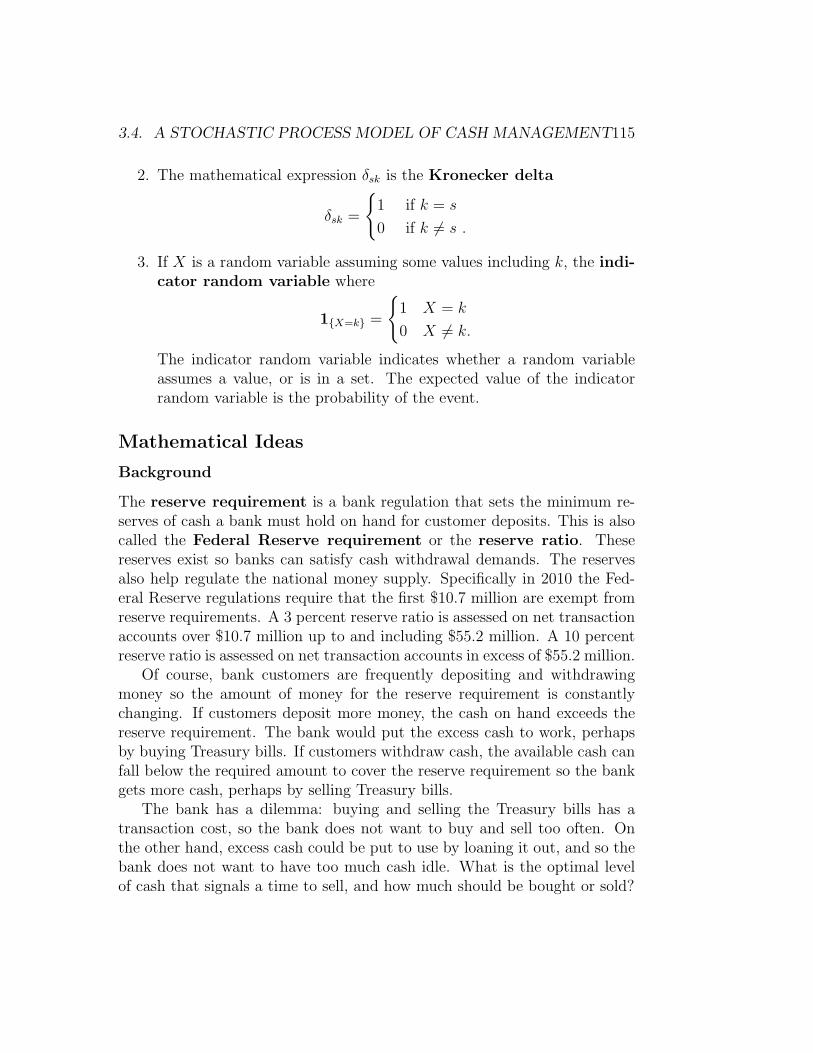
3.4. A STOCHASTIC PROCESS MODEL OF CASH MANAGEMENT115
2. The mathematical expression δsk is the Kronecker delta
δsk =
1 if k = s
0 if k 6= s .
3. If X is a random variable assuming some values including k, the indi-cator random variable where
1X=k =
1 X = k
0 X 6= k.
The indicator random variable indicates whether a random variableassumes a value, or is in a set. The expected value of the indicatorrandom variable is the probability of the event.
Mathematical Ideas
Background
The reserve requirement is a bank regulation that sets the minimum re-serves of cash a bank must hold on hand for customer deposits. This is alsocalled the Federal Reserve requirement or the reserve ratio. Thesereserves exist so banks can satisfy cash withdrawal demands. The reservesalso help regulate the national money supply. Specifically in 2010 the Fed-eral Reserve regulations require that the first $10.7 million are exempt fromreserve requirements. A 3 percent reserve ratio is assessed on net transactionaccounts over $10.7 million up to and including $55.2 million. A 10 percentreserve ratio is assessed on net transaction accounts in excess of $55.2 million.
Of course, bank customers are frequently depositing and withdrawingmoney so the amount of money for the reserve requirement is constantlychanging. If customers deposit more money, the cash on hand exceeds thereserve requirement. The bank would put the excess cash to work, perhapsby buying Treasury bills. If customers withdraw cash, the available cash canfall below the required amount to cover the reserve requirement so the bankgets more cash, perhaps by selling Treasury bills.
The bank has a dilemma: buying and selling the Treasury bills has atransaction cost, so the bank does not want to buy and sell too often. Onthe other hand, excess cash could be put to use by loaning it out, and so thebank does not want to have too much cash idle. What is the optimal levelof cash that signals a time to sell, and how much should be bought or sold?

116CHAPTER 3. FIRST STEP ANALYSIS FOR STOCHASTIC PROCESSES
Modeling
We assume for a simple model that a bank’s cash level fluctuates randomly asa result of many small deposits and withdrawals. We model this by dividingtime into successive, equal length periods, each of short duration. The peri-ods might be weekly, the reporting period the Federal Reserve Bank requiresfor some banks. In each time period, assume the reserve randomly increasesor decreases one unit of cash, perhaps measured in units of $100,000, eachwith probability 1/2. That is, in period n, the change in the banks reservesis
Yn =
+1 with probability 1/2
−1 with probability 1/2.
The equal probability assumption simplifies calculations for this model. It ispossible to relax the assumption to the case p 6= q, but we will not do thishere.
Let T0 = s be the initial cash on hand. Then Tn = T0 +∑n
j=1 Yj is thetotal cash on hand at period n.
The bank will intervene if the reserve gets too small or too large. Againfor simple modeling, if the reserve level drops to zero, the bank sells assetssuch as Treasury bonds to replenish the reserve back up to s. If the cash levelever increases to S, the bank buys Treasury bonds to reduce the reserves tos. What we have modeled here is a version of the Gambler’s Ruin, exceptthat when this “game” reaches the “ruin” or “victory” boundaries, 0 or Srespectively, the “game” immediately restarts again at s.
Now the cash level fluctuates in a sequence of cycles or games. Each cyclebegins with s units of cash on hand and ends with either a replenishment ofcash, or a reduction of cash.
Mean number of visits to a particular state
Now let k be one of the possible reserve states with 0 < k < S and let Wsk
be the expected number of visits to the level k up to the ending time of thecycle starting from s. A formal mathematical expression for this expressionis
Wsk = E
[N−1∑j=1
1Tj=k
]

3.4. A STOCHASTIC PROCESS MODEL OF CASH MANAGEMENT117
Figure 3.3: Several typical cycles in a model of the reserve requirement.
where 1Tj=k is the indicator random variable where
1Tj=k =
1 Tj = k
0 Tj 6= k.
Note that the inner sum is a random sum, since it depends on the length ofthe cycle N , which is cycle dependent.
Then using first-step analysis Wsk satisfies the equations
Wsk = δsk +1
2Ws−1,k +
1
2Ws+1,k
with boundary conditions W0k = WSk = 0. The term δsk is the Kroneckerdelta
δsk =
1 if k = s
0 if k 6= s.
The explanation of this equation is very similar to the derivation of theequation for the expected duration of the coin-tossing game. The terms12Ws−1,k + 1
2Ws+1,k arise from the standard first-step analysis or expectation-
by-conditioning argument for Wsk. The non-homogeneous term in the prior

118CHAPTER 3. FIRST STEP ANALYSIS FOR STOCHASTIC PROCESSES
expected duration equation (which is +1) arises because the game will alwaysbe at least 1 step longer after the first step. In the current equation, the δsknon-homogeneous term arises because the number of visits to level k afterthe first step will be 1 more if k = s but the number of visits to level k afterthe first step will be 0 more if k 6= s.
For the ruin probabilities, the difference equation was homogeneous, andwe only needed to find the general solution. For the expected duration,the difference equation was non-homogeneous with a non-homogeneous termwhich was the constant 1, making the particular solution reasonably easy tofind. Now the non-homogeneous term depends on the independent variable,so solving for the particular solution will be more involved.
First we find the general solutionW hsk to the homogeneous linear difference
equation
W hsk =
1
2W hs−1,k +
1
2W hs+1,k.
This is easy, we already know that it is W hsk = A+Bs.
Then we must find a particular solution W psk to the non-homogeneous
equation
W psk = δsk +
1
2W ps−1,k +
1
2W ps+1,k.
For purposes of guessing a plausible particular solution, temporarily re-writethe equation as
−2δsk = W ps−1,k − 2W p
sk +W ps+1,k.
The expression on the right is a centered second difference. For the priorexpected duration equation, we looked for a particular solution with a con-stant centered second difference. Based on our experience with functions itmade sense to guess a particular solution of the form C+Ds+Es2 and thensubstitute to find the coefficients. Here we seek a function whose centeredsecond difference is 0 except at k where the second difference jumps to 1.This suggests the particular solution is piecewise linear, say
W psk =
C +Ds if s ≤ k
E + Fs if s > k.
In the exercises, we verify that the solution of this set of equations is
W psk =
0 if s < k
2(k − s) if s ≥ k.

3.4. A STOCHASTIC PROCESS MODEL OF CASH MANAGEMENT119
We can write this as W psk = −2 max(s− k, 0)
Then solving for the boundary conditions, the full solution is
Wsk = 2 [s(1− k/S)−max(s− k, 0)] .
Expected Duration and Expected Total Cash in a Cycle
Consider the first passage time N when the reserves first reach 0 or S, sothat cycle ends and the bank intervenes to change the cash reserves. Thevalue of N is a random variable, it depends on the sample path. We arefirst interested in Ds = E [N ], the expected duration of a cycle. From theprevious section we already know Ds = s(S − s).
Next, we are interested in the mean cost of holding cash on hand duringa cycle i, starting from amount s. Call this mean Ws. Let r be the cost perunit of cash, per unit of time. We then obtain the cost by weighting Wsk,the mean number of times the cash is at number of units k starting froms, multiplying by k, multiplying by the factor r and summing over all theavailable amounts of cash:
Ws =S−1∑k=1
rkWsk
= 2
[s
S
S−1∑k=1
rk(S − k)−s−1∑k=1
rk(s− k)
]
= 2
[s
S
[rS(S − 1)(S + 1)
6
]− rs(s− 1)(s+ 1)
6
]= r
s
3
[S2 − s2
].
These results are interesting and useful in their own right as estimates ofthe length of a cycle and the expected cost of cash on hand during a cycle.Now we use these results to evaluate the long run behavior of the cycles. Uponresetting the cash at hand to s when the amount of cash reaches 0 orS, thecycles are independent of each of the other cycles because of the assumptionof independence of each step. Let K be the fixed cost of the buying or sellingof the treasury bonds to start the cycle, let Ni be the random length of thecycle i, and let Ri be the total opportunity cost of holding cash on handduring cycle i. Then the cost over n cycles is nK +R1 + · · ·+Rn. Divide by

120CHAPTER 3. FIRST STEP ANALYSIS FOR STOCHASTIC PROCESSES
n to find the average cost
Expected total cost in cycle i = K + E [Ri] ,
but we have another expression for the expectation E [Ri],
Expected opportunity cost = E [Ri] = rs
3
[S2 − s2
].
Likewise the total length of n cycles is N1 + · · · + Nn. Divide by n to findthe average length,
Expected length =N1 + · · ·+Nn
n= s(S − s).
These expected values allow us to calculate the average costs
Long run average cost, dollars per week =K + E [Ri]
E [Ni].
Then E [Ri] = rWs and E [Ni] = s(S − s). Therefore
Long run average cost, dollars per week =K + (1/3)rs(S2 − s2)
s(S − s).
Simplify the analysis by setting x = s/S so that the expression of interest is
Long run average cost =K + (1/3)rS3x(1− x2)
S2x(1− x).
Remark. Aside from being a good thing to non-dimensionalize the modelas much as possible, it also appears that optimizing the original long runcost average in the original variables S and s is messy and difficult. Thisof course would not be known until you had tried it. However, knowing theoptimization is difficult in variables s and S additionally motivates makingthe transformation to the non-dimensional ratio x = s/S.
Now we have a function in two variables that we wish to optimize. Takethe partial derivatives with respect to x and S and set them equal to 0, thensolve, to find the critical points.
The results are that
xopt =1
3
Sopt = 3
(3K
4r
) 13
.

3.4. A STOCHASTIC PROCESS MODEL OF CASH MANAGEMENT121
That is, the optimal value of the maximum amount of cash to keep varies asthe cube root of the cost ratios, and the reset amount of cash is 1/3 of thatamount.
Criticism of the model
The first test of the model would be to look at the amounts S and s for well-managed banks and determine if the banks are using optimal values. Thatis, one could do a statistical survey of well-managed banks and determineif the values of S vary as the cube root of the cost ratio, and if the restartvalue is 1/3 of that amount. Of course, this assumes that the model is validand that banks are following the predictions of the model, either consciouslyor not.
This model is too simple and could be modified in a number of ways.One change might be to change the reserve requirements to vary with thelevel of deposits, just as the 2010 Federal Reserve requirements vary. Addingadditional reserve requirement levels to the current model adds a level ofcomplexity, but does not substantially change the level of mathematics in-volved.
The most important change would be to allow the changes in depositsto have a continuous distribution instead of jumping up or down by oneunit in each time interval. Modification to continuous time would make themodel more realistic instead of changing the cash at discrete time intervals.The assumption of statistical independence from time step to time step isquestionable, and so could also be relaxed. All these changes require deeperanalysis and more sophisticated stochastic processes.
Sources
This section is adapted from: Section 6.1.3 and 6.2, pages 157-164 in AnIntroduction to Stochastic Modeling, [50].
Problems to Work for Understanding
1. Find a particular solution W psk to the non-homogeneous equation
W psk = δsk +
1
2W ps−1,k +
1
2W ps+1,k.
122CHAPTER 3. FIRST STEP ANALYSIS FOR STOCHASTIC PROCESSES
using the trial function
W psk =
C +Ds if s ≤ k
E + Fs if s > k.
2. Show that
Ws =S−1∑k=1
kWsk
= 2
[s
S
S−1∑k=1
k(S − k)−s−1∑k=1
k(s− k)
]
= 2
[s
S
[S(S − 1)(S + 1)
6
]− s(s− 1)(s+ 1)
6
]=s
3
[S2 − s2
]You will need formulas for
∑Nk=1 k and
∑Nk=1 k
2 or alternatively for∑Nk=1 k(M − k). These are easily found or derived.
3. (a) For the long run average cost
C =K + (1/3)rS3x(1− x2)
S2x(S − x).
find ∂C/∂x.
(b) For the long run average cost
C =K + (1/3)rS3x(1− x2)
S2x(1− x).
find ∂C/∂S.
(c) Find the optimum values of x and S.
Outside Readings and Links:
1. Milton Friedman: The Purpose of the Federal Reserve system. Thereaction of the Federal Reserve system at the beginning of the GreatDepression.

Chapter 4
Limit Theorems for StochasticProcesses
4.1 Laws of Large Numbers
Rating
Mathematically Mature: may contain mathematics beyond calculus withproofs.
Section Starter Question
Consider a fair (p = 1/2 = q) coin tossing game carried out for 1000 tosses.Explain in a sentence what the “law of averages” says about the outcomesof this game.
Key Concepts
1. The precise statement, meaning and proof of the Weak Law of LargeNumbers.
2. The precise statement and meaning of the Strong Law of Large Num-bers.
123

124CHAPTER 4. LIMIT THEOREMS FOR STOCHASTIC PROCESSES
Vocabulary
1. The Weak Law of Large Numbers is a precise mathematical state-ment of what is usually loosely referred to as the “law of averages”.Precisely, let X1, . . . , Xn be independent, identically distributed ran-dom variables each with mean µ and variance σ2. Let Sn = X1+· · ·+Xn
and consider the sample mean or more loosely, the “average” Sn/n.Then the Weak Law of Large Numbers says that the sample mean Sn/nconverges in probability to the population mean µ. That is:
limn→∞
Pn [|Sn/n− µ| > ε] = 0
In words, the proportion of those samples whose sample mean differssignificantly from the population mean diminishes to zero as the samplesize increases.
2. The Strong Law of Large Numbers says that Sn/n converges to µwith probability 1. That is:
P[
limn→∞
Sn/n = µ]
= 1
In words, the Strong Law of Large Numbers “almost every” samplemean approaches the population mean as the sample size increases.
Mathematical Ideas
The Weak Law of Large Numbers
Lemma 3 (Markov’s Inequality). If X is a random variable that takes onlynonnegative values, then for any a > 0:
P [X ≥ a] ≤ E [X] /a
Proof. Here is a proof for the case where X is a continuous random variable

4.1. LAWS OF LARGE NUMBERS 125
with probability density f :
E [X] =
∫ ∞0
xf(x) dx
=
∫ a
0
xf(x) dx+
∫ ∞a
xf(x) dx
≥∫ ∞a
xf(x) dx
≥∫ ∞a
af(x) dx
= a
∫ ∞a
f(x) dx
= aP [X ≥ a] .
(The proof for the case where X is a purely discrete random variable issimilar with summations replacing integrals. The proof for the general caseis exactly as given with dF (x) replacing f(x) dx and interpreting the integralsas Riemann-Stieltjes integrals.)
Lemma 4 (Chebyshev’s Inequality). If X is a random variable with finitemean µ and variance σ2, then for any value k > 0:
P [|X − µ| ≥ k] ≤ σ2/k2.
Proof. Since (X−µ)2 is a nonnegative random variable, we can apply Markov’sinequality (with a = k2) to obtain
P[(X − µ)2 ≥ k2
]≤ E
[(X − µ)2
]/k2.
But since (X − µ)2 ≥ k2 if and only if |X − µ| ≥ k, the inequality above isequivalent to:
P [|X − µ| ≥ k] ≤ σ2/k2
and the proof is complete.
Theorem 5 (Weak Law of Large Numbers). Let X1, X2, X3, . . . , be indepen-dent, identically distributed random variables each with mean µ and varianceσ2. Let Sn = X1 + · · ·+Xn. Then Sn/n converges in probability to µ. Thatis:
limn→∞
P [|Sn/n− µ| > ε] = 0.
126CHAPTER 4. LIMIT THEOREMS FOR STOCHASTIC PROCESSES
Proof. Since the mean of a sum of random variables is the sum of the means,and scalars factor out of expectations:
E [Sn/n] = (1/n)n∑i=1
E [Xi] = (1/n)(nµ) = µ.
Since the variance of a sum of independent random variables is the sum ofthe variances, and scalars factor out of variances as squares:
Var [Sn/n] = (1/n2)n∑i
Var [Xi] = (1/n2)(nσ2) = σ2/n.
Fix a value ε > 0. Then using elementary definitions for probability measureand Chebyshev’s Inequality:
0 ≤ Pn [|Sn/n− µ| > ε] ≤ Pn [|Sn/n− µ| ≥ ε] ≤ σ2/(nε2).
Then by the squeeze theorem for limits
limn→∞
P [|Sn/n− µ| > ε] = 0.
Jacob Bernoulli originally proved the Weak Law of Large Numbers in 1713for the special case when the Xi are binomial random variables. Bernoullihad to create an ingenious proof to establish the result, since Chebyshev’sinequality was not known at the time. The theorem then became known asBernoulli’s Theorem. Simeon Poisson proved a generalization of Bernoulli’sbinomial Weak Law and first called it the Law of Large Numbers. In 1929the Russian mathematician Aleksandr Khinchin proved the general form ofthe Weak Law of Large Numbers presented here. Many other versions of theWeak Law are known, with hypotheses that do not require such stringentrequirements as being identically distributed, and having finite variance.
The Strong Law of Large Numbers
Theorem 6 (Strong Law of Large Numbers). Let X1, X2, X3, . . . , be indepen-dent, identically distributed random variables each with mean µ and varianceE[X2j
]<∞. Let Sn = X1 + · · ·+Xn. Then Sn/n converges with probability
1 to µ,
P[
limn→∞
Snn
= µ
]= 1.

4.1. LAWS OF LARGE NUMBERS 127
The proof of this theorem is beautiful and deep, but would take us too farafield to prove it. The Russian mathematician Andrey Kolmogorov provedthe Strong Law in the generality stated here, culminating a long series ofinvestigations through the first half of the 20th century.
Discussion of the Weak and Strong Laws of Large Numbers
In probability theory a theorem that tells us how a sequence of probabilitiesconverges is called a weak law. For coin tossing, the sequence of probabilitiesis the sequence of binomial probabilities associated with the first n tosses.The Weak Law of Large Numbers says that if we take n large enough, thenthe binomial probability of the mean over the first n tosses differing “much”from the theoretical mean should be small. This is what is usually popularlyreferred to as the law of averages. However, this is a limit statement and theWeak law of Large Numbers above does not indicate the rate of convergence,nor the dependence of the rate of convergence on the difference ε. Notefurthermore that the Weak Law of Large Numbers in no way justifies thefalse notion called the “Gambler’s Fallacy”, namely that a long string ofsuccessive Heads indicates a Tail “is due to occur soon”. The independenceof the random variables completely eliminates that sort of prescience.
A strong law tells how the sequence of random variables as a samplepath behaves in the limit. That is, among the infinitely many sequences(or paths) of coin tosses we select one “at random” and then evaluate thesequence of means along that path. The Strong Law of Large Numbers saysthat with probability 1 that sequence of means along that path will convergeto the theoretical mean. The formulation of the notion of probability on aninfinite (in fact an uncountably infinite) sample space requires mathematicsbeyond the scope of the course, partially accounting for the lack of a prooffor the Strong Law here.
Note carefully the difference between the Weak Law of Large Numbersand the Strong Law. We do not simply move the limit inside the probability.These two results express different limits. The Weak Law is a statementthat the group of finite-length experiments whose sample mean is close tothe population mean approaches all of the possible experiments as the lengthincreases. The Strong Law is an experiment-by-experiment statement, it says(almost every) sequence has a sample mean that approaches the populationmean. Weak laws are usually much easier to prove than strong laws.

128CHAPTER 4. LIMIT THEOREMS FOR STOCHASTIC PROCESSES
Sources
This section is adapted from Chapter 8, “Limit Theorems”, A First Coursein Probability, by Sheldon Ross, Macmillan, 1976.
Problems to Work for Understanding
1. Suppose X is a continuous random variable with mean and varianceboth equal to 20. What can be said about P [0 ≤ X ≤ 40]?
2. Suppose X is an exponentially distributed random variable with meanE [X] = 1. For x = 0.5, 1, and 2, compare P [X ≥ x] with the Markovinequality bound.
3. Suppose X is a Bernoulli random variable with P [X = 1] = p andP [X = 0] = 1− p = q. Compare P [X ≥ 1] with the Markov inequalitybound.
4. Let X1, X2, . . . , X10 be independent Poisson random variables withmean 1. First use the Markov Inequality to get a bound on P [X1 + · · ·+X10 > 15].Next find the exact probability that P [X1 + · · ·+X10 > 15] using thatthe fact that the sum of independent Poisson random variables withparameters λ1, λ2 is again Poisson with parameter λ1 + λ2.
Outside Readings and Links:
1. Virtual Laboratories in Probability and Statistics. Search the pagefor Weak Law and then run the Binomial Coin Experiment and theMatching Experiment.
2.
4.2 Moment Generating Functions
Rating
Mathematically Mature: may contain mathematics beyond calculus withproofs.

4.2. MOMENT GENERATING FUNCTIONS 129
Section Starter Question
Give some examples of transform methods in mathematics, science or engi-neering that you have seen or used and explain why transform methods areuseful.
Key Concepts
1. The moment generating function converts problems about prob-abilities and expectations into problems from calculus about functionvalues and derivatives.
2. The value of the nth derivative of the moment generating functionevaluated at 0 is the value of the nth moment of X.
3. The sum of independent normal random variables is again a normalrandom variable whose mean is the sum of the means, and whose vari-ance is the sum of the variances.
Vocabulary
1. The nth moment of the random variable X is E [Xn] =∫xxnf(x) dx
(provided this integral converges absolutely.)
2. The moment generating function φX(t) is defined by
φX(t) = E[etX]
=
∑i etxip(xi) if X is discrete∫
xetxf(x) dx if X is continuous
for all values t for which the integral converges.
Mathematical Ideas
We need some tools to aid in proving theorems about random variables. Inthis section we develop a tool called the moment generating functionwhich converts problems about probabilities and expectations into prob-lems from calculus about function values and derivatives. Moment gener-ating functions are one of the large class of transforms in mathematics that

130CHAPTER 4. LIMIT THEOREMS FOR STOCHASTIC PROCESSES
Xi,E [Xi] ,P [Xi] −→ φX(t)yconclusions ←− calculations
Figure 4.1: Block diagram of transform methods.
turn a difficult problem in one domain into a manageable problem in an-other domain. Other examples are Laplace transforms, Fourier transforms,Z-transforms, generating functions, and even logarithms.
The general method can be expressed schematically in the diagram:
Expectation of Independent Random Variables
Lemma 7. If X and Y are independent random variables, then for anyfunctions g and h:
E [g(X)h(Y )] = E [g(X)] E [h(Y )]
Proof. To make the proof definite suppose that X and Y are jointly contin-uous, with joint probability density function F (x, y). Then:
E [g(X)h(Y )] =
∫∫(x,y)
g(x)h(y)f(x, y) dx dy
=
∫x
∫y
g(x)h(y)fX(x)fY (y) dx dy
=
∫x
g(x)fX(x) dx
∫y
h(y)fY (y) dy
= E [g(X)] E [h(Y )] .
The Moment Generating Function
The moment generating function φX(t) is defined by
φX(t) = E[etX]
=
∑i etxip(xi) if X is discrete∫
xetxf(x) dx if X is continuous

4.2. MOMENT GENERATING FUNCTIONS 131
for all values t for which the integral converges.
Example. The degenerate probability distribution has all the probabilityconcentrated at a single point. That is, if X is a degenerate random variablewith the degenerate probability distribution, then X = µ with probability 1and X is any other value with probability 0. That is, the degenerate randomvariable is a discrete random variable exhibiting certainty of outcome. Themoment generating function of the degenerate random variable is particularlysimple: ∑
xi=µ
exit = eµt.
If the moments of order k exist for 0 ≤ k ≤ k0, then the moment gen-erating function is continuously differentiable up to order k0 at t = 0. Themoments of X can be generated from φX(t) by repeated differentiation:
φ′X =d
dtE[etX]
=d
dt
∫x
etxfX(x) dx
=
∫x
d
dtetxfX(x) dx
=
∫x
xetxfX(x) dx
= E[XetX
].
Thenφ′X(0) = E [X] .
Likewise
φ′′X(t) =d
dtφ′X(t)
=d
dt
∫x
xetxfX(x) dx
=
∫x
xd
dtetxfX(x) dx
=
∫x
x2etxfX(x) dx
= E[X2etX
].
132CHAPTER 4. LIMIT THEOREMS FOR STOCHASTIC PROCESSES
Then
φ′′X(0) = E[X2].
Continuing in this way:
φ(n)X (0) = E [Xn]
In words: the value of the nth derivative of the moment generating functionevaluated at 0 is the value of the nth moment of X.
Theorem 8. If X and Y are independent random variables with momentgenerating functions φX(t) and φY (t) respectively, then φX+Y (t), the momentgenerating function of X + Y is given by φX(t)φY (t). In words, the momentgenerating function of a sum of independent random variables is the productof the individual moment generating functions.
Proof. Using the lemma on independence above:
φX+Y (t) = E[et(X+Y )
]= E
[etXetY
]= E
[etX]E[etY]
= φX(t)φY (t).
Theorem 9. If the moment generating function is defined in a neighborhoodof t = 0 then the moment generating function uniquely determines the prob-ability distribution. That is, there is a one-to-one correspondence betweenthe moment generating function and the distribution function of a randomvariable, when the moment-generating function is defined and finite.
Proof. This proof is too sophisticated for the mathematical level we havenow.
The moment generating function of a normal random variable
Theorem 10. If Z ∼ N(µ, σ2), then φZ(t) = exp(µt+ σ2t2/2).
4.2. MOMENT GENERATING FUNCTIONS 133
Proof.
φZ(t) = E[etX]
=1√
2πσ2
∫ ∞−∞
etxe−(x−µ)2/(2σ2) dx
=1√
2πσ2
∫ ∞−∞
exp
(−(x2 − 2µx+ µ2 − 2σ2tx)
2σ2
)dx
Now by the technique of completing the square:
x2 − 2µx+ µ2 − 2σ2tx = x2 − 2(µ+ σ2t)x+ µ2
= (x− (µ+ σ2t))2 − (µ+ σ2t)2 + µ2
= (x− (µ+ σ2t))2 − σ4t2 − 2µσ2t
So returning to the calculation of the m.g.f.
φZ(t) =1√
2πσ2
∫ ∞−∞
exp
(− ((x− (µ+ σ2t))2 − σ4t2 − 2µσ2t)
2σ2
)dx
=1√
2πσ2exp
(σ4t2 + 2µσ2t
2σ2
)∫ ∞−∞
exp
(−(x− (µ+ σ2t))2
2σ2
)dx
= exp
(σ4t2 + 2µσ2t
2σ2
)= exp
(µt+ σ2t2/2
)Theorem 11. If Z1 ∼ N(µ1, σ
21), and Z2 ∼ N(µ2, σ
22) and Z1 and Z2 are
independent, then Z1 + Z2 ∼ N(µ1 + µ2, σ21 + σ2
2). In words, the sum ofindependent normal random variables is again a normal random variablewhose mean is the sum of the means, and whose variance is the sum of thevariances.
Proof. We compute the moment generating function of the sum using ourtheorem about sums of independent random variables. Then we recognize theresult as the moment generating function of the appropriate normal randomvariable.
φZ1+Z2(t) = φZ1(t)φZ2(t)
= exp(µ1t+ σ21t
2/2) exp(µ2t+ σ22t
2/2)
= exp((µ1 + µ2)t+ (σ21 + σ2
2)t2/2)
134CHAPTER 4. LIMIT THEOREMS FOR STOCHASTIC PROCESSES
An alternative visual proof that the sum of independent normal randomvariables is again a normal random variable using only calculus is The Sumof Independent Normal Random Variables is Normal
Sources
This section is adapted from: Introduction to Probability Models, by SheldonRoss.
Problems to Work for Understanding
1. Calculate the moment generating function of a random variable Xhaving a uniform distribution on [0, 1]. Use this to obtain E [X] andVar [X].
2. Calculate the moment generating function of a discrete random vari-able X having a geometric distribution. Use this to obtain E [X] andVar [X].
Outside Readings and Links:
1. http://www.math.uah.edu/stat/expect/Generating.xhtml
2. http://mathworld.wolfram.com/Moment-GeneratingFunction.html in Math-World.com
4.3 The Central Limit Theorem
Rating
Mathematically Mature: may contain mathematics beyond calculus withproofs.
Section Starter Question
What is the most important probability distribution? Why do you choosethat distribution as most important?
4.3. THE CENTRAL LIMIT THEOREM 135
Key Concepts
1. The statement, meaning and proof of the Central Limit Theorem.
2. We expect the normal distribution to arise whenever the numericaldescription of a state of a system results from numerous small randomadditive effects, with no single or small group of effects dominant.
Vocabulary
1. The Central Limit Theorem: Suppose that for a sequence of inde-pendent, identically distributed random variables Xi, each Xi has finitevariance σ2. Let
Zn = (Sn − nµ)/(σ√n) = (1/σ)(Sn/n− µ)
√n
and let Z be the “standard” normally distributed random variable withmean 0 and variance 1. Then Zn converges in distribution to Z, thatis:
limn→∞
Pr[Zn ≤ a] =
∫ a
−∞
1√2π
exp(−u2/2) du
In words, a shifted and rescaled sample distribution is approximatelystandard normal.
Mathematical Ideas
Convergence in Distribution
Lemma 12. Let X1, X2, . . . be a sequence of random variables having cu-mulative distribution functions FXn and moment generating functions φXn.Let X be a random variable having cumulative distribution function FXand moment generating function φX . If φXn(t) → φX(t), for all t, thenFXn(t)→ FX(t) for all t at which FX(t) is continuous.
We say that the sequence Xi converges in distribution to X and wewrite
XiD→ X.
Notice that P [a < Xi ≤ b] = FXi(b)−FXi
(a)→ F (b)−F (a) = P [a < X ≤ b],so convergence in distribution implies convergence of probabilities of events.
136CHAPTER 4. LIMIT THEOREMS FOR STOCHASTIC PROCESSES
Likewise, convergence of probabilities of events implies convergence in distri-bution.
This lemma is useful because it is fairly routine to determine the pointwiselimit of a sequence of functions using ideas from calculus. It is usually mucheasier to check the pointwise convergence of the moment generating func-tions than it is to check the convergence in distribution of the correspondingsequence of random variables.
We won’t prove this lemma, since it would take us too far afield intothe theory of moment generating functions and corresponding distributiontheorems. However, the proof is a fairly routine application of ideas from themathematical theory of real analysis.
Application: Weak Law of Large Numbers.
Here’s a simple representative example of using the convergence of the mo-ment generating function to prove a useful result. We will prove a version ofthe Weak Law of Large numbers that does not require the finite variance ofthe sequence of independent, identically distributed random variables.
Theorem 13 (Weak Law of Large Numbers). Let X1, . . . , Xn be indepen-dent, identically distributed random variables each with mean µ and such thatE [|X|] is finite. Let Sn = X1 + · · ·+Xn. Then Sn/n converges in probabilityto µ. That is:
limn→∞
P [|Sn/n− µ| > ε] = 0
Proof. If we denote the moment generating function of X by φ(t), then themoment generating function of
Snn
=n∑i=1
Xi
n
is (φ(t/n))n. The existence of the first moment assures us that φ(t) is dif-ferentiable at 0 with a derivative equal to µ. Therefore, by tangent-lineapproximation (first-degree Taylor polynomial approximation)
φ
(t
n
)= 1 + µ
t
n+ r2(t/n)

4.3. THE CENTRAL LIMIT THEOREM 137
where r2(t/n) is a error term such that
limn→∞
r(t/n)
(1/n)= 0.
Then we need to consider
φ
(t
n
)n= (1 + µ
t
n+ r2(t/n))n.
Taking the logarithm of (1 + µ(t/n) + r(t/n))n and using L’Hospital’s Rule,we see that
φ(t/n)n → exp(µt).
But this last expression is the moment generating function of the (degenerate)point mass distribution concentrated at µ. Hence,
limn→∞
P [|Sn/n− µ| > ε] = 0
The Central Limit Theorem
Theorem 14 (Central Limit Theorem). Let random variables X1, . . . Xn
• be independent and identically distributed,
• have common mean E [Xi] = µ and common variance Var [Xi] = σ2,
• the common moment generating function φXi(t) = E [etxi ] exists and is
finite in a neighborhood of t = 0.
Consider Sn =∑n
i=1Xi. Let
•Zn = (Sn − nµ)/(σ
√n) = (1/σ)(Sn/n− µ)
√n,
• Z be the standard normally distributed random variable with mean 0and variance 1.
Then Zn converges in distribution to Z, that is:
limn→∞
P [Zn ≤ a] =
∫ a
−∞(1/√
2π) exp(−u2/2) du.

138CHAPTER 4. LIMIT THEOREMS FOR STOCHASTIC PROCESSES
Remark. The Central Limit Theorem is true even under the slightly weakerassumptions that X1, . . . Xn only are independent and identically distributedwith finite mean µ and finite variance σ2 without the assumption that mo-ment generating function exists. However, the proof below using momentgenerating functions is simple and direct enough to justify using the addi-tional hypothesis.
Proof. Assume at first that µ = 0 and σ2 = 1. Assume also that the momentgenerating function of the Xi, (which are identically distributed, so there isonly one m.g.f) is φX(t), exists and is everywhere finite. Then the m.g.f ofXi/√n is
φX/√n(t) = E[exp(tXi/
√n)]
= φX(t/√n).
Recall that the m.g.f of a sum of independent r.v.s is the product of them.g.f.s. Thus the m.g.f of Sn/
√n is (note that here we used µ = 0 and
σ2 = 1)φSn/
√n(t) = [φX(t/
√n)]n
The quadratic approximation (second-degree Taylor polynomial expansion)of φX(t) at 0 is by calculus:
φX(t) = φX(0) + φ′X(0)t+ (φ′′X(0)/2)t2 + r3(t) = 1 + t2/2 + r3(t)
again since E [X] = φ′(0) is assumed to be 0 and Var [X] = E [X2] −(E [X])2 = φ′′(0) − (φ′(0))2 = φ′′(0) is assumed to be 1. Here r3(t) is anerror term such that limt→0 r3(t)/t
2 = 0. Thus,
φ(t/√n) = 1 + t2/(2n) + r3(t/
√n)
implying thatφSn/
√n = [1 + t2/(2n) + r3(t/
√n)]n.
Now by some standard results from calculus,
[1 + t2/(2n) + r3(t/√n)]n → exp(t2/2)
as n → ∞. (If the reader needs convincing, it’s computationally easier toshow that
n log(1 + t2/(2n) + r3(t/√n))→ t2/2,
using L’Hospital’s Rule in order to account for the r3(t) term.)To handle the general case, consider the standardized random variables
(Xi − µ)/σ, each of which now has mean 0 and variance 1 and apply theresult.
4.3. THE CENTRAL LIMIT THEOREM 139
The first version of the central limit theorem was proved by Abraham deMoivre around 1733 for the special case when the Xi are binomial randomvariables with p = 1/2 = q. This proof was subsequently extended by Pierre-Simon Laplace to the case of arbitrary p 6= q. Laplace also discovered themore general form of the Central Limit Theorem presented here. His proofhowever was not completely rigorous, and in fact, cannot be made completelyrigorous. A truly rigorous proof of the Central Limit Theorem was firstpresented by the Russian mathematician Aleksandr Liapunov in 1901-1902.As a result, the Central Limit Theorem (or a slightly stronger version of theCentral Limit Theorem) is occasionally referred to as Liapunov’s theorem.A theorem with weaker hypotheses but with equally strong conclusion isLindeberg’s Theorem of 1922. It says that the sequence of random variablesneed not be identically distributed, but instead need only have zero means,and the individual variances are small compared to their sum.
Accuracy of the Approximation by the Central Limit Theorem
The statement of the Central Limit Theorem does not say how good theapproximation is. One rule of thumb is that the approximation given by theCentral Limit Theorem applied to a sequence of Bernoulli random trials orequivalently to a binomial random variable is acceptable when np(1 − p) >18 [31, page 34], [42, page 134]. The normal approximation to a binomialdeteriorates as the interval (a, b) over which the probability is computedmoves away from the binomial’s mean value np. Another rule of thumb isthat the normal approximation is acceptable when n ≥ 30 for all “reasonable”probability distributions.
The Berry-Esseen Theorem gives an explicit bound: For independent,identically distributed random variables Xi with µ = E [Xi] = 0, σ2 = E [X2
i ],and ρ = E [|X3|], then∣∣∣∣P [Sn/(σ√n) < a
]−∫ a
−∞
1√2πe−u
2/2 du
∣∣∣∣ ≤ 33
4
ρ
σ3
1√n.
Illustration 1
In Figure 4.2 is a graphical illustration of the Central Limit Theorem. Moreprecisely, this is an illustration of the de Moivre-Laplace version, the approx-imation of the binomial distribution with the normal distribution.

140CHAPTER 4. LIMIT THEOREMS FOR STOCHASTIC PROCESSES
Figure 4.2: Approximation of the binomial distribution with the normaldistribution.
The figure is actually an non-centered and unscaled illustration since thebinomial random variable Sn is not shifted by the mean, nor normalized tounit variance. Therefore, the binomial and the corresponding approximatingnormal are both centered at E [Sn] = np. The variance of the approximatingnormal is σ2 =
√npq and the widths of the bars denoting the binomial
probabilities are all unit width, and the heights of the bars are the actualbinomial probabilities.
Illustration 2
From the Central Limit Theorem we expect the normal distribution applieswhenever an outcome results from numerous small additive effects with nosingle or small group of effects dominant. Here is a standard illustration ofthat principle.
Consider the following data from the National Longitudinal Survey ofYouth (NLSY). This study started with 12,000 respondents aged 14-21 yearsin 1979. By 1994, the respondents were aged 29-36 years and had 15,000children among them. Of the respondents 2,444 had exactly two children.In these 2,444 families, the distribution of children was boy-boy: 582; girl-girl 530, boy-girl 666, and girl-boy 666. It appears that the distribution ofgirl-girl family sequences is low compared to the other combinations, ourintuition tells us that all combinations are equally likely and should appearin roughly equal proportions. We will assess this intuition with the CentralLimit Theorem.
Consider a sequence of 2,444 trials with each of the two-child families.
4.3. THE CENTRAL LIMIT THEOREM 141
Let Xi = 1 (success) if the two-child family is girl-girl, and Xi = 0 (failure)if the two-child family is otherwise. We are interested in the probabilitydistribution of
S2444 =2444∑i=1
Xi.
In particular, we are interested in the probability P [S2444 ≤ 530], that is,what is the probability of seeing as few as 530 girl-girl families or even fewerin a sample of 2444 families? We can use the Central Limit Theorem toestimate this probability.
We are assuming the family “success” variables Xi are independent, andidentically distributed, a reasonable but arguable assumption. Nevertheless,without this assumption, we cannot justify the use of the Central LimitTheorem, so we adopt the assumption. Then µ = E [Xi] = (1/4) · 1 +(3/4) · 0 = 1/4 and Var [Xi] = (1/4)(3/4) = 3/16 so σ =
√3/4 Note that
2444 · (1/4) · (3/4) = 45.75 > 18 so the rule of thumb justifies the use of theCentral Limit Theorem. Hence
P [S2444 ≤ 530] = P[S2444 − 2444 · (1/4)
(√
3/4 ·√
2444)≤ 530− 2444 · (1/4)
(√
3/4 ·√
2444)
]≈ P [Z ≤ −3.7838]
≈ 0.0000772
It is highly unlikely that under our assumptions such a proportion would haveoccurred. Therefore, we are justified in thinking that under our assumptions,the actual proportion of girl-girl families is low. We then begin to suspect ourassumptions, one of which was the implicit assumption that the appearanceof girls was equally likely as boys, leading to equal proportions of the fourtypes of families. In fact, there is ample evidence that the birth of boys ismore likely than the birth of girls.
Illustration 3
We expect the normal distribution to apply whenever the numerical descrip-tion of a state of a system results from numerous small additive effects, withno single or small group of effects dominant. Here is another illustration ofthat principle.
The Central Limit Theorem can be used to assess risk. Two large bankscompete for customers to take out loans. The banks have comparable of-
142CHAPTER 4. LIMIT THEOREMS FOR STOCHASTIC PROCESSES
ferings. Assume that each bank has a certain amount of funds available forloans to customers. Any customers seeking a loan beyond the available fundswill cost the bank, either as a lost opportunity cost, or because the bank it-self has to borrow to secure the funds to lend to the customer. If too fewcustomers take out loans then that also costs the bank since now the bankhas unused funds.
We create a simple mathematical model of this situation. We supposethat the loans are all of equal size and for definiteness each bank has fundsavailable for a certain number (to be determined) of these loans. Then sup-pose n customers select a bank independently and at random. Let Xi = 1if customer i selects bank H with probability 1/2 and Xi = 0 if customersselect bank T, also with probability 1/2. Then Sn =
∑ni=1Xi is the number
of loans from bank H to customers. Now there is some positive probabil-ity that more customers will turn up than can be accommodated. We canapproximate this probability with the Central Limit Theorem:
P [Sn > s] = P[(Sn − n/2)/((1/2)
√n) > (s− n/2)/((1/2)
√n)]
≈ P[Z > (s− n/2)/((1/2)
√n)]
= P[Z > (2s− n)/
√n]
Now if n is large enough that this probability is less than (say) 0.01, then thenumber of loans will be sufficient in 99 of 100 cases. Looking up the value ina normal probability table,
2s− n√n
> 2.33
so if n = 1000, then s = 537 will suffice. If both banks assume the same riskof sellout at 0.01, then each will have 537 for a total of 1074 loans, of which74 will be unused. In the same way, if the bank is willing to assume a riskof 0.20, i.e. having enough loans in 80 of 100 cases, then they would needfunds for 514 loans, and if the bank wants to have sufficient loans in 999 outof 1000 cases, the bank should have 549 loans available.
Now the possibilities for generalization and extension are apparent. Afirst generalization would be allow the loan amounts to be random with somedistribution. Still we could apply the Central Limit Theorem to approximatethe demand on available funds. Second, the cost of either unused funds orlost business could be multiplied by the chance of occurring. The total ofthe products would be an expected cost, which could then be minimized.

4.3. THE CENTRAL LIMIT THEOREM 143
Sources
The proofs in this section are adapted from Chapter 8, “Limit Theorems”,A First Course in Probability, by Sheldon Ross, Macmillan, 1976. Furtherexamples and considerations come from Heads or Tails: An Introductionto Limit Theorems in Probability, by Emmanuel Lesigne, American Mathe-matical Society, Chapter 7, pages 29–74. Illustration 2 is adapted from AnIntroduction to Probability Theory and Its Applications, Volume I, secondedition, William Feller, J. Wiley and Sons, 1957, Chapter VII. Illustration1 is adapted from Dicing with Death: Chance, Health, and Risk by StephenSenn, Cambridge University Press, Cambridge, 2003.
Problems to Work for Understanding
1. Let X1, X2, . . . , X10 be independent Poisson random variables withmean 1. First use the Markov Inequality to get a bound on Pr[X1 +· · ·+X10 > 15]. Next use the Central Limit theorem to get an estimateof Pr[X1 + · · ·+X10 > 15].
2. A first simple assumption is that the daily change of a company’s stockon the stock market is a random variable with mean 0 and variance σ2.That is, if Sn represents the price of the stock on day n with S0 given,then
Sn = Sn−1 +Xn, n ≥ 1
where X1, X2, . . . are independent, identically distributed continuousrandom variables with mean 0 and variance σ2. (Note that this is anadditive assumption about the change in a stock price. In the binomialtree models, we assumed that a stock’s price changes by a multiplicativefactor up or down. We will have more to say about these two distinctmodels later.) Suppose that a stock’s price today is 100. If σ2 = 1,what can you say about the probability that after 10 days, the stock’sprice will be between 95 and 105 on the tenth day?
3. Suppose you bought a stock at a price b + c, where c > 0 and thepresent price is b. (Too bad!) You have decided to sell the stock after30 more trading days have passed. Assume that the daily change of thecompany’s stock on the stock market is a random variable with mean0 and variance σ2. That is, if Sn represents the price of the stock on
144CHAPTER 4. LIMIT THEOREMS FOR STOCHASTIC PROCESSES
day n with S0 given, then
Sn = Sn−1 +Xn, n ≥ 1
where X1, X2, . . . are independent, identically distributed continuousrandom variables with mean 0 and variance σ2. Write an expressionfor the probability that you do not recover your purchase price.
4. If you buy a lottery ticket in 50 independent lotteries, and in eachlottery your chance of winning a prize is 1/100, write down and evaluatethe probability of winning and also approximate the probability usingthe Central Limit Theorem.
(a) exactly one prize,
(b) at least one prize,
(c) at least two prizes.
Explain with a reason whether or not you expect the approximation tobe a good approximation.
5. Find a number k such that the probability is about 0.6 that the numberof heads obtained in 1000 tossings of a fair coin will be between 440and k.
6. Find the moment generating function φX(t) = E [exp(tX)] of the ran-dom variable X which takes values 1 with probability 1/2 and −1with probability 1/2. Show directly (that is, without using Taylorpolynomial approximations) that φX(t/
√n)n → exp(t2/2). (Hint: Use
L’Hospital’s Theorem to evaluate the limit, after taking logarithms ofboth sides.)
7. A bank has $1,000,000 available to make for car loans. The loans arein random amounts uniformly distributed from $5,000 to $20,000. Howmany loans can the bank make with 99% confidence that it will haveenough money available?
8. An insurance company is concerned about health insurance claims.Through an extensive audit, the company has determined that over-statements (claims for more health insurance money than is justified bythe medical procedures performed) vary randomly with an exponential
4.4. THE ABSOLUTE EXCESS OF HEADS OVER TAILS 145
distribution X with a parameter 1/100 which implies that E [X] = 100and Var [X] = 1002. The company can afford some overstatements sim-ply because it is cheaper to pay than it is to investigate and counter-claim to recover the overstatement. Given 100 claims in a month, thecompany wants to know what amount of reserve will give 95% cer-tainty that the overstatements do not exceed the reserve. (All unitsare in dollars.) What assumptions are you using?
Outside Readings and Links:
1. Virtual Laboratories in Probability and Statistics. Search the page forBinomial approximation and then run the Binomial Timeline Experi-ment.
2. Central Limit Theorem explanation Pretty good visual explanation ofthe application of the Central Limit Theorem to sampling means.
3. Central Limit Theorem explanation Another lecture demonstration ofthe application of the Central Limit Theorem to sampling means.
4.4 The Absolute Excess of Heads over Tails
Rating
Mathematically Mature: may contain mathematics beyond calculus withproofs.
Section Starter Question
What does the law of averages have to say about the probability of having afixed lead of say 20 Heads or more over Tails or 20 Tails or more over Headsat the end of a coin flipping game of some fixed duration? What does theWeak Law of Large Numbers have to say about having a fixed lead? Whatdoes the Weak Law have to say about having a proportional lead, say 1%?What does the Central Limit Theorem have to say about the lead?
146CHAPTER 4. LIMIT THEOREMS FOR STOCHASTIC PROCESSES
Key Concepts
1. The probability that the number of heads exceeds the number of tails orthe number of tails exceeds the number of heads in a sequence of coin-flips by some fixed amount can be estimated with the Central LimitTheorem and the probability gets close to 1 as the number of tossesgrows large.
2. The probability that the number of heads exceeds the number of tailsor the number of tails exceeds the number of heads in a sequence ofcoin-flips by some fixed proportion can be estimated with the CentralLimit Theorem and the probability gets close to 0 as the number oftosses grows large.
Vocabulary
1. The half-integer correction, also called the continuity correctionarises because the distribution of the binomial distribution is a discretedistribution, while the standard normal distribution is a continuousdistribution.
Mathematical Ideas
Introduction
Probability theory generally has two classes of theorems about the results ofcoin-tossing games and therefore random walks:
1. Those theorems that tell how well-behaved and natural are the out-comes of typical coin-tossing games and random walks. The Weak Lawof Large Numbers, the Strong Law of Large Numbers and the CentralLimit Theorem fall into this category.
2. Those theorems that tell how strange and unnatural are the outcomesof typical coin-tossing games and random walks. The Arcsine Law andthe Law of the Iterated Logarithm are good examples in this category.
In this section we will ask two related questions about the net fortune ina coin-tossing game:
4.4. THE ABSOLUTE EXCESS OF HEADS OVER TAILS 147
1. What is the probability of an excess of a fixed number of heads overtails or tails over heads at some fixed time in the coin-flipping game?
2. What is the probability that the number of heads exceeds the numberof tails or the number of tails exceeds the number of heads by somefixed fraction of the number of tosses?
Using the Central Limit Theorem, we will be able to provide precise answersto each question and then to apply the ideas to interesting questions ingambling and finance.
The Half-Integer Correction to the Central Limit Theorem
Often when using the Central Limit Theorem to approximate a discrete dis-tribution, especially the binomial distribution, we adopt the half-integercorrection, also called the continuity correction. The correction arisesbecause the binomial distribution has a discrete distribution while the stan-dard normal distribution has a continuous distribution. For any integer sand real value h with 0 ≤ h < 1 the binomial random variable Sn hasP [|Sn| ≤ s] = P [|Sn| ≤ s+ h], yet the corresponding Central Limit Theoremapproximation with the standard normal cumulative distribution function,P [|Z| ≤ (s+ h)/
√n] increases as h increases from 0 to 1. It is customary to
take h = 1/2 to interpolate the difference. This choice is also justified bylooking at the approximation of the binomial with the normal.
Symbolically, the half-integer correction to the Central Limit Theorem is
P [a ≤ Sn ≤ b] ≈∫ ((b+1/2)−np)/√npq
((a−1/2)−np)/√npq
1√2π
exp(−u2/2)du
= P [((a− 1/2)− np)/√npq ≤ Z ≤ ((b+ 1/2)− np)/√npq]
for integers a and b.
The absolute excess of heads over tails
Consider the sequence of independent random variables Yi which take values1 with probability 1/2 and −1 with probability 1/2. This is a mathematicalmodel of a fair coin flip game where a 1 results from “heads” on the ithcoin toss and a −1 results from “tails”. Let Hn and Ln be the number ofheads and tails respectively in n flips. Then Tn =
∑ni=1 Yi = Hn−Ln counts
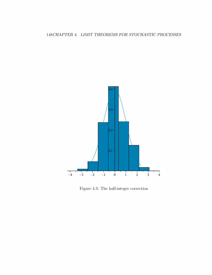
148CHAPTER 4. LIMIT THEOREMS FOR STOCHASTIC PROCESSES
Figure 4.3: The half-integer correction
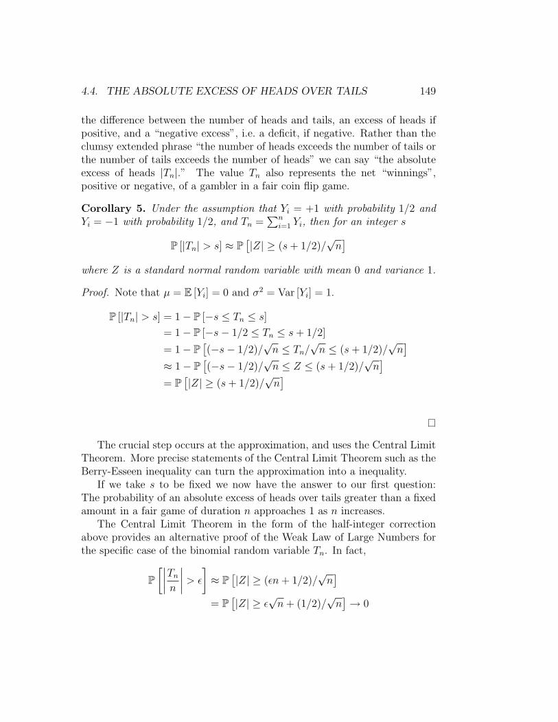
4.4. THE ABSOLUTE EXCESS OF HEADS OVER TAILS 149
the difference between the number of heads and tails, an excess of heads ifpositive, and a “negative excess”, i.e. a deficit, if negative. Rather than theclumsy extended phrase “the number of heads exceeds the number of tails orthe number of tails exceeds the number of heads” we can say “the absoluteexcess of heads |Tn|.” The value Tn also represents the net “winnings”,positive or negative, of a gambler in a fair coin flip game.
Corollary 5. Under the assumption that Yi = +1 with probability 1/2 andYi = −1 with probability 1/2, and Tn =
∑ni=1 Yi, then for an integer s
P [|Tn| > s] ≈ P[|Z| ≥ (s+ 1/2)/
√n]
where Z is a standard normal random variable with mean 0 and variance 1.
Proof. Note that µ = E [Yi] = 0 and σ2 = Var [Yi] = 1.
P [|Tn| > s] = 1− P [−s ≤ Tn ≤ s]
= 1− P [−s− 1/2 ≤ Tn ≤ s+ 1/2]
= 1− P[(−s− 1/2)/
√n ≤ Tn/
√n ≤ (s+ 1/2)/
√n]
≈ 1− P[(−s− 1/2)/
√n ≤ Z ≤ (s+ 1/2)/
√n]
= P[|Z| ≥ (s+ 1/2)/
√n]
The crucial step occurs at the approximation, and uses the Central LimitTheorem. More precise statements of the Central Limit Theorem such as theBerry-Esseen inequality can turn the approximation into a inequality.
If we take s to be fixed we now have the answer to our first question:The probability of an absolute excess of heads over tails greater than a fixedamount in a fair game of duration n approaches 1 as n increases.
The Central Limit Theorem in the form of the half-integer correctionabove provides an alternative proof of the Weak Law of Large Numbers forthe specific case of the binomial random variable Tn. In fact,
P[∣∣∣∣Tnn
∣∣∣∣ > ε
]≈ P
[|Z| ≥ (εn+ 1/2)/
√n]
= P[|Z| ≥ ε
√n+ (1/2)/
√n]→ 0

150CHAPTER 4. LIMIT THEOREMS FOR STOCHASTIC PROCESSES
as n→∞.
Rewriting P[∣∣Tn
n
∣∣ > ε]
= P [|Tn| > εn] this restatement of the Weak Lawactually provides the answer to our second question: The probability thatthe absolute excess of heads over tails is greater than a fixed fraction of theflips in a fair game of duration n approaches 0 as n increases.
Finally, this gives an estimate on the central probability in a binomialdistribution.
Corollary 6.
P [Tn = 0] ≈ P[|Z| < (1/2)/
√n]→ 0
as n→∞.
We can estimate this further
P[|Z| < (1/2)/
√n]
=1√2π
∫ 1/(2√n)
−1/(2√n)
e−u2/2 du
=1√2π
∫ 1/(2√n)
−1/(2√n)
1− u2/2 + u4/8 + . . . du
=1√2π
1√n− 1
24√
2π
1
n3/2+
1
640√
2π
1
n5/2+ . . . .
So we see that P [Tn = 0] goes to zero at the rate of 1/√n.
Illustration 1
What is the probability that the number of heads exceeds the number of tailsby more than 20 or the number of tails exceeds the number of heads by morethan 20 after 500 tosses of a fair coin? By the proposition, this is:
P [|Tn| > 20] ≈ P[|Z| ≥ 20.5/
√500]
= 0.3477.
This is a reasonably large probability, and is larger than many people wouldexpect.
Here is a graph of the probability of at least s excess heads in 500 tossesof a fair coin:

4.4. THE ABSOLUTE EXCESS OF HEADS OVER TAILS 151
Figure 4.4: Probability of s excess heads in 500 tosses
Illustration 2
What is the probability that there is “about the same number of heads astails” in 500 tosses? Here we interpret “about the same” as within 5, that is,an absolute difference of 1% or less of the number of tosses. Note that since500 is even, so the difference in the number of heads and tails cannot be anodd number, so must be either 0, 2 or 4.
P [|S500| < 5] ≈ P[|Z| ≤ 5.5/
√500]
= 0.1943
so it would be somewhat unusual (in that it occurs in less than 20% of games)to have the number of heads and tails so close.
Illustration 3
Suppose you closely follow a stock recommendation source whose methodsare based on technical analysis. You accept every bit of advice from thissource about trading stocks. You choose 10 stocks to buy, sell or hold everyday based on the recommendations. Each day for each stock you will gainor lose money based on the advice. Note that it is possible to gain moneyeven if the advice says the stocks will decrease in value, say by short-sellingor using put options. How good can this strategy be? We will make this

152CHAPTER 4. LIMIT THEOREMS FOR STOCHASTIC PROCESSES
vague question precise by asking “How good does the information from thetechnical analysis have to be so that the probability of losing money over ayear’s time is 1 in 10,000?”
The 10 stocks over 260 business days in a year means that there 2,600daily gains or losses. Denote each daily gain or loss as Xi, if the advice iscorrect you will gain Xi > 0 and if the advice is wrong you will lose Xi < 0.We want the total change Xannual =
∑2600i=1 Xi > 0 and we will measure that
by asking that P [Xannual < 0] be small. In the terms of this section, we areinterested in the complementary probability of an excess of successes overfailures.
We assume that the changes are random variables, identically distributed,independent and the moments of all the random variables are finite. Wewill make specific assumptions about the distribution later, for now theseassumptions are sufficient to apply the Central Limit Theorem. Then thetotal change Xannual =
∑2600i=1 Xi is approximately normally distributed with
mean µ = 2600 · E [X1] and variance σ2 = 2600 · Var [X1]. Note that hereagain we are using the uncentered and unscaled version of the Central LimitTheorem. In symbols
P
[a ≤
2600∑i=1
Xi ≤ b
]≈ 1√
2πσ2
∫ b
a
exp
(−(u− µ)2
2σ2
)du.
We are interested in
P
[2600∑i=1
Xi ≤ 0
]≈ 1√
2πσ2
∫ 0
−∞exp
(−(u− µ)2
2σ2
)du.
By the change of variables v = (u− µ)/σ, we can rewrite the probability as
P [Xannual ≤ 0] =1√2π
∫ −µ/σ−∞
exp(−v2/2
)dv = Φ
(−µσ
)so that the probability depends only on the ratio −µ/σ. We desire thatΦ(−µ/σ) = P [Xannual < 0] 1/10,000. Then we can solve for −µ/σ ≈ −3.7.Since µ = 2600·E [X1] and σ2 = 2600·Var [X1], we calculate that for the totalannual change to be a loss we must have E [X1] ≈ (3.7/
√2600) ·
√Var [X1] =
0.07 ·√
Var [X1].
Now we consider what the requirement E [X1] = 0.07 ·√
Var [X1] meansfor specific distributions. If we assume that the individual changesXi are nor-mally distributed with a positive mean, then we can use E [X1] /
√Var [X1] =
4.4. THE ABSOLUTE EXCESS OF HEADS OVER TAILS 153
0.07 to calculate that P [X1] < 0 ≈ 0.47210, or about 47%. Alternatively,if we assume that the individual changes Xi are binomial random variableswith P [X1 = 1] = p, then E [X1] = 2p− 1 and Var [X1] = 4p(1− p). We canuse 2p − 1 = E [X1] = 0.07 Var [X1] = 0.07 · (4p(1 − p)) to solve for p. Theresult is p = 0.53491.
In either case, this means that any given piece of advice only has to havea 53% chance of being correct in order to have a perpetual money-makingmachine. Compare this with the strategy of using a coin flip to provide theadvice. Since we don’t observe any perpetual money-making machines, weconclude that any advice about stock picking must be less than 53% reliableor about the same as flipping a coin.
Now suppose that instead we have a computer algorithm predicting stockmovements for all publicly traded stocks, of which there are about 2,000.Suppose further that we wish to restrict the chance that P [Xannual] < 10−6,that is 1 chance in a million. Then we can repeat the analysis to show thatthe computer algorithm would only need to have P [X1] < 0 ≈ 0.49737,practically indistinguishable from a coin flip, in order to make money. Thisprovides a statistical argument against the utility of technical analysis forstock price prediction. Money-making is not sufficient evidence to distinguishability in stock-picking from coin-flipping.
Sources
This section is adapted from the article “Tossing a Fair Coin” by LeonardLipkin. The discussion of the continuity correction is adapted from PartialSums and the Central Limit Theorem in the Virtual Laboratories in Prob-ability and Statistics. The third example in this section is adapted from apresentation by Jonathan Kaplan of D.E. Shaw and Co. in summer 2010.
Problems to Work for Understanding
1. (a) What is the approximate probability that the number of heads iswithin 10 of the number of tails, that is, a difference of 2% or lessof the number of tosses in 500 tosses?
(b) What is the approximate probability that the number of heads iswithin 20 of the number of tails, that is, a difference of 4% or lessof the number of tosses in 500 tosses?

154CHAPTER 4. LIMIT THEOREMS FOR STOCHASTIC PROCESSES
(c) What is the approximate probability that the number of heads iswithin 25 of the number of tails, that is, a difference of 5% or lessof the number of tosses in 500 tosses?
(d) Derive and then graph a simple power function that gives theapproximate probability that the number of heads is within x ofthe number of tails in 500 tosses, for 0 ≤ x ≤ 500.
2. (a) What is the probability that the number of heads is within 10of the number of tails, that is, a difference of 1% or less of thenumber of tosses in 1000 tosses?
(b) What is the probability that the number of heads is within 10of the number of tails, that is, a difference of 0.5% or less of thenumber of tosses in 2000 tosses?
(c) What is the probability that the number of heads is within 10of the number of tails, that is, a difference of 0.2% or less of thenumber of tosses in 5000 tosses?
(d) Derive and then graph a simple power function that gives theapproximate probability that the number of heads is within x ofthe number of tails in 500 tosses, for 0 ≤ x ≤ 500.
3. Derive the rate, as a function of n, that the probability of heads exceedstails by a fixed value s approaches 1 as n→∞.
4. Derive the rate, as a function of n, that the probability of heads exceedstails by a fixed fraction ε approaches 0 as n→∞.
Outside Readings and Links:
1. Virtual Laboratories in Probability and Statistics. Search the page forRandom Walk Simulation and run the Last Visit to Zero experiment.
2. Virtual Laboratories in Probability and Statistics. Search the page forBallot Experiment and run the Ballot Experiment.

Chapter 5
Brownian Motion
5.1 Intuitive Introduction to Diffusions
Rating
Mathematically Mature: may contain mathematics beyond calculus withproofs.
Section Starter Question
Suppose you wanted to display the function y =√x on a graphing calculator.
Describe the process necessary to choose a proper window to display thegraph.
Key Concepts
1. The passage from discrete random walks to continuous stochastic pro-cesses, from the probability point of view and the partial differentialequation point of view.
Vocabulary
1. A diffusion process, or a diffusion for short, is a Markov processfor which all sample functions are continuous. It is also a solution to astochastic differential equation.
155

156 CHAPTER 5. BROWNIAN MOTION
Mathematical Ideas
The question is “How should we set up the limiting process so that we canmake a continuous time limit of the discrete time random walk?” Firstwe consider a discovery approach to this question by asking what shouldbe the limiting process which assures us that we can visualize the limitingprocess. Next we take a probabilistic view using the Central Limit Theoremto justify the limiting process to pass from a discrete probability distributionto a probability density function. Finally, we consider the limiting processderived from passing from the difference equation from first-step analysis toa differential equation.
Visualizing Limits of Random Walks
The Random Walk
Consider a random walk starting at the origin. The nth step takes the walkerto the position Tn = Y1 + · · · + Yn, the sum of n independent, identicallydistributed Bernoulli random variables Yi assuming the values +1, and −1with probabilities p and q respectively. Then recall that the mean of a sumof random variables is the sum of the means:
E [Tn] = (p− q)n
and the variance of a sum of independent random variables is the sum of thevariances:
Var [Tn] = 4pqn.
Trying to use the mean to derive the limit
Now suppose we want to display a motion picture of the random walk movingleft and right along the x-axis. This would be a motion picture of the “phasespace” diagram of the random walk. Suppose we want the motion picture todisplay 1 million steps and be a reasonable length of time, say 1000 seconds,between 16 and 17 minutes. This fixes the time scale at a rate of one stepper millisecond. What should be the window in the screen in order to geta good sense of the random walk? For this question, we use a fixed unit ofmeasurement, say centimeters, for the width of the screen and the individualsteps. Let δ be the length of the steps. To find the window to display the

5.1. INTUITIVE INTRODUCTION TO DIFFUSIONS 157
random walk on the axis, we then need to know the size of δTn. Now
E [δ · Tn] = (p− q) · δ · n
andVar [δ · Tn] = 4 · p · q · δ2 · n.
We want n to be large (about 1 million) and to see the walk on the screenwe want the expected end place to be comparable to the screen size, say 30cm. That is,
E [δ · Tn] = (p− q) · δ · n < δ · n ≈ 30cm
so δ must be 3 · 10−5cm = 0.0003mm to get the end point on the screen. Butthen the movement of the walk measured by the standard deviation√
Var [δ · Tn] ≤ δ ·√n = 3× 10⁻² cm
will be so small as to be indistinguishable. We will not see any randomvariations!
Trying to use the variance to derive the limit
Let us turn the question around: We want to see the variations in many-steprandom walks, so the standard deviations must be a reasonable fraction Dof the screen size √
Var [δ · Tn] ≤ δ ·√n ≈ D · 30 cm .
This is possible if δ = D · 3 × 10⁻² cm . We still want to be able to see theending expected position which will be
E [δ · Tn] = (p− q) · δ · n = (p− q) ·D · 3× 104cm.
To be consistent with the variance requirement this will only be possibleif (p − q) ≈ 10−2. That is, p − q must be comparable in magnitude toδ = 3× 10⁻².
The limiting process
Now generalize these results to visualize longer and longer walks in a fixedamount or time. Since δ → 0 as n → ∞, then likewise (p − q) → 0, while
158 CHAPTER 5. BROWNIAN MOTION
p + q = 1, so p → 1/2. The analytical formulation of the problem is asfollows. Let δ be the size of the individual steps, let r be the number of stepsper unit time. We ask what happens to the random walk in the limit whereδ → 0, r →∞, and p→ 1/2 in such a manner that:
(p− q) · δ · r → c
and4 · p · q · δ2 · r → D.
Probabilistic Solution of the Limit Question
In our accelerated random walk, consider the nth step at time t = n/r andconsider the position on the line x = k · δ. Let
vk,n = P [Tn = k]
be the probability that the nth step is at position k. We are interested in theprobability of finding the walk at given instant t and in the neighborhood ofa given point x, so we investigate the limit of vk,n as n/r → t, and k · δ → x.
Remember that the random walk can only reach an even-numbered posi-tion after an even number of steps, and an odd-numbered position after anodd number of steps. Therefore in all cases n + k is even and (n + k)/2 isan integer. Likewise n − k is even and (n − k)/2 is and integer. We reachposition k at time step n if the walker takes (n + k)/2 steps to the rightand (n − k)/2 steps to the left. The mix of steps to the right and the leftcan be in any order. So the walk reaches position k at step n with binomialprobability
vk,n =
(n
(n+ k)/2
)· p(n+k)/2 · q(n−k)/2
From the Central Limit Theorem
vk,n ∼ (1/(√
2 · π · p · q)) · exp(−[(n+ k)/2− n · p]2/(2 · π · n · pq))= (1/(
√2π · pq)) · exp(−[k − n(p− q)]2/(8πnpq))
∼ ((2δ)/(√
2πDt)) exp(−[x− ct]2/(2Dt))
5.1. INTUITIVE INTRODUCTION TO DIFFUSIONS 159
Since vk,n is the probability of finding Tn ·δ between k ·δ and (k+2)·δ, andsince this interval has length 2 ·δ we can say that the ratio vk,n/(2δ) measureslocally the probability per unit length, that is the probability density. Thelast relation above implies that the ratio vk,n/n tends to
v(t, x) = ((2 · δ)/(√
2 · πDt)) exp(−[x− ct]2/(2Dt))
It follows by the definition of integration as the sums of quantities repre-senting densities times geometric lengths or areas, that sums of probabilitiesvk,n can be approximated by integrals and the result may be restated as
P [a < Tnδ < b]→ (1/(√
2πDt))
∫ b
a
exp(−(x− ct)2/(Dt))
The integral on the right may be expressed in terms of the standard normaldistribution function.
Note that we derived the limiting approximation of the binomial distri-bution
vk,n ∼ ((2δ)/(√
2πDt)) exp(−[x− ct]2/(2Dt))
by applying the general form of the Central Limit Theorem. However, itis possible to derive this limit directly through careful analysis. The directderivation is known as the DeMoivre-Laplace Theorem and it is the mostbasic form of the Central Limit Theorem.
Differential Equation Solution of the Limit Question
Another method is to start from the difference equations governing the ran-dom walk, and then pass to the differential equation in the limit. We canthen obviously generalize the differential equations, and find out that thedifferential equations govern well-defined stochastic processes depending oncontinuous time. Since differential equations have a well-developed theoryand many tools to manipulate, transform and solve them, this method turnsout to be useful.
Consider the position of the walker in the random walk at the nth and(n+ 1)st trial. Through a first step analysis the probabilities vk,n satisfy thedifference equations:
vk,n+1 = p · vk−1,n + q · vk+1,n

160 CHAPTER 5. BROWNIAN MOTION
In the limit as k →∞ and n→∞, vk,n will be the sampling of the functionv(t, x) at time intervals r, so that kr = t, and space intervals so that n · δ =x. That is, the function v(t, x) should be an approximate solution of thedifference equation:
v(t+ r−1, x) = pv(t, x− δ) + qv(t, x+ δ)
We assume v(t, x) is a smooth function so that we can expand v(t, x) in aTaylor series at any point. Using the first order approximation in the timevariable on the left, and the second-order approximation on the right in thespace variable, we get (after canceling the leading terms v(t, x) )
∂v(t, x)
∂t= (q − p) · δr∂v(t, x)
∂x+ (1/2)δ2r
∂2v(t, x)
∂x2
In our passage to the limit, the omitted terms of higher order tend to zero,so may be neglected. The remaining coefficients are already accounted for inour limits and so the equation becomes:
∂v(t, x)
∂t= −c∂v(t, x)
∂x+ (1/2)D
∂2v(t, x)
∂x2
This is a special diffusion equation, more specifically, a diffusion equationwith convective or drift terms, also known as the Fokker-Planck equation fordiffusion. It is a standard problem to solve the differential equation for v(t, x)and therefore, we can find the probability of being at a certain position at acertain time. One can verify that
v(t, x) = (1/(√
2πDt)) exp(−[x− ct]2/(2Dt))
is a solution of the diffusion equation, so we reach the same probabilitydistribution for v(t, x).
The diffusion equation can be immediately generalized by permitting thecoefficients c and D to depend on x, and t. Furthermore, the equationpossesses obvious analogues in higher dimensions and all these generalizationcan be derived from general probabilistic postulates. We will ultimatelydescribe stochastic processes related to these equations as diffusions.
Sources
This section is adapted from W. Feller, in Introduction to Probability Theoryand Applications, Volume I, Chapter XIV, page 354.

5.2. THE DEFINITION OF BROWNIAN MOTION AND THE WIENER PROCESS161
Problems to Work for Understanding
1. Consider a random walk with a step to right having probability p anda step to the left having probability q. The step length is δ. Thewalk is taking r steps per minute. What is the rate of change of theexpected final position and the rate of change of the variance? Whatmust we require on the quantities p, q, r and delta in order to see theentire random walk with more and more steps at a fixed size in a fixedamount of time?
2. Verify the limit taking to show that
vk,n ∼ (1/(√
2πDt)) exp(−[x− ct]2/(2Dt)).
3. Show that
v(t, x) = (1/(√
2πDt)) exp(−[x− ct]2/(2Dt))
is a solution of
∂v(t, x)
∂t= −c∂v(t, x)
∂x+ (1/2)D
∂2v(t, x)
∂x2
by substitution.
Outside Readings and Links:
1. Brownian Motion in Biology. A simulation of a random walk of a sugarmolecule in a cell.
2. Virtual Laboratories in Probability and Statistics. Search the page forRandom Walk experiment.
5.2 The Definition of Brownian Motion and
the Wiener Process
Rating
Mathematically Mature: may contain mathematics beyond calculus withproofs.

162 CHAPTER 5. BROWNIAN MOTION
Section Starter Question
Some mathematical objects are defined by a formula or an expression. Someother mathematical objects are defined by their properties, not explicitly byan expression. That is, the objects are defined by how they act, not by whatthey are. Can you name a mathematical object defined by its properties?
Key Concepts
1. We define Brownian motion in terms of the normal distribution of theincrements, the independence of the increments, and the value at 0.
2. The joint density function for the value of Brownian motion at severaltimes is a multivariate normal distribution.
Vocabulary
1. Brownian Motion is the physical phenomenon named after the En-glish botanist Robert Brown who discovered it in 1827. Brownian mo-tion is the zig-zagging motion exhibited by a small particle, such as agrain of pollen, immersed in a liquid or a gas. The first explanationof this phenomenon was given by Albert Einstein in 1905. He showedthat Brownian motion could be explained by assuming the immersedparticle was constantly buffeted by the actions of the molecules of thesurrounding medium. Since then the abstracted process has been usedbeneficially in such areas as analyzing price levels in the stock marketand in quantum mechanics.
2. The Wiener process is the mathematical definition and abstraction ofthe physical process as a stochastic process. The American mathemati-cian Norbert Wiener gave the definition and properties in a series ofpapers starting in 1918. Generally, the terms Brownian motion andWiener process are the same, although Brownian motion emphasizesthe physical aspects and Wiener process emphasizes the mathematicalaspects.
3. Bachelier process is an uncommonly applied term meaning the samething as Brownian motion and Wiener process. In 1900, Louis Bachelierintroduced the limit of random walk as a model for the prices on the

5.2. THE DEFINITION OF BROWNIAN MOTION AND THE WIENER PROCESS163
Paris stock exchange, and so is the originator of the idea of what is nowcalled Brownian motion. This term is occasionally found in financialliterature and European usage.
Mathematical Ideas
Definition of Wiener Process
Previously, we have considered a discrete time random process, that is, attimes n = 1, 2, 3, . . . corresponding to coin flips, we have a sequence of randomvariables Tn. We are now going to consider a continuous time random process,that is a function Wt which is a random variable at each time t ≥ 0. To sayWt is a random variable at each time is too general so we must put someadditional restrictions on our process to have something interesting to study.
Definition (Wiener Process). The Standard Wiener Process is a stochas-tic process W (t), for t ≥ 0, with the following properties:
1. Every increment W (t)−W (s) over an interval of length t−s is normallydistributed with mean 0 and variance t− s, that is
W (t)−W (s) ∼ N(0, t− s)
2. For every pair of disjoint time intervals [t1, t2] and [t3, t4], with t1 <t2 ≤ t3 < t4, the increments W (t4) − W (t3) and W (t2) − W (t1) areindependent random variables with distributions given as in part 1, andsimilarly for n disjoint time intervals where n is an arbitrary positiveinteger.
3. W (0) = 0
4. W (t) is continuous for all t.
Note that property 2 says that if we know W (s) = x0, then the indepen-dence (and W (0) = 0) tells us that no further knowledge of the values ofW (τ) for τ < s has any additional effect on our knowledge of the probabilitylaw governing W (t) − W (s) with t > s. More formally, this says that if0 ≤ t0 < t1 < . . . < tn < t, then
P [W (t) ≥ x|W (t0) = x0,W (t1) = x1, . . .W (tn) = xn] = P [W (t) ≥ x|W (tn) = xn]

164 CHAPTER 5. BROWNIAN MOTION
This is a statement of the Markov property of the Wiener process.Recall that the sum of independent random variables which are respec-
tively normally distributed with mean µ1 and µ2 and variances σ21 and σ2
2 is anormally distributed random variable with mean µ1+µ2 and variance σ2
1 +σ22,
see Moment Generating Functions Therefore for increments W (t3) −W (t2)and W (t2)−W (t1) the sum W (t3)−W (t2)+W (t2)−W (t1) = W (t3)−W (t1) isnormally distributed with mean 0 and variance t3−t1 as we expect. Property2 of the definition is consistent with properties of normal random variables.
Let
p(x, t) =1√2πt
exp(−x2/(2t))
denote the probability density for a N(0, t) random variable. Then to derivethe joint density of the event
W (t1) = x1,W (t2) = x2, . . .W (tn) = xn
with t1 < t2 < . . . < tn, it is equivalent to know the joint probability densityof the equivalent event
W (t1)−W (0) = x1,W (t2)−W (t1) = x2−x1, . . . ,W (tn)−W (tn−1) = xn−xn−1.
Then by part 2, we immediately get the expression for the joint probabilitydensity function:
f(x1, t1;x2, t2; . . . ;xn, tn) = p(x1, t)p(x2−x1, t2−t1) . . . p(xn−xn−1, tn−tn−1)
Comments on Modeling Security Prices with the Wiener Process
A plot of security prices over time and a plot of one-dimensional Brownianmotion versus time has least a superficial resemblance.
If we were to use Brownian motion to model security prices (ignoringfor the moment that some security prices are better modeled with the moresophisticated geometric Brownian motion rather than simple Brownian mo-tion) we would need to verify that security prices have the 4 definitionalproperties of Brownian motion.
1. The assumption of normal distribution of stock price changes seems tobe a reasonable first assumption. Figure 5.2 illustrates this reasonable

5.2. THE DEFINITION OF BROWNIAN MOTION AND THE WIENER PROCESS165
Figure 5.1: Graph of the Dow-Jones Industrial Average from August, 2008to August 2009 (blue line) and a random walk with normal increments withthe same mean and variance (brown line).
Figure 5.2: A standardized density histogram of daily close-to-close returnson the Pepsi Bottling Group, symbol NYSE:PBG, from September 16, 2003to September 15, 2003, up to September 13, 2006 to September 12, 2006
166 CHAPTER 5. BROWNIAN MOTION
agreement. The Central Limit Theorem provides a reason to believethe agreement, assuming the requirements of the Central Limit The-orem are met, including independence. Unfortunately, although thefigure shows what appears to be reasonable agreement a more rigorousstatistical analysis shows that the data distribution does not matchnormality.
Another good reason for still using the assumption of normality for theincrements is that the normal distribution is easy to work with. Theprobability density is easy to work with, the cumulative distribution istabulated, the moment-generating function is easy to use, and the sumof independent normal distributions is again normal. A substitutionof another distribution is possible but makes the resulting stochasticprocess models very difficult to work with, and beyond the scope ofthis treatment.
Moreover, this assumption ignores the small possibility that negativestock prices could result from a large negative change. This is notreasonable (and the log normal distribution from geometric Brownianmotion which avoids this possibility is a better model).
Moreover, the assumption of a constant variance on different intervalsof the same length is not a good assumption since stock volatility itselfseems to be volatile. That is, the variance of a stock price changes andneed not be proportional to the length of the time interval.
2. The assumption of independent increments seems to be a reasonable as-sumption, at least on a long enough term. From second to second, priceincrements are probably correlated. From day to day, price incrementsare probably independent. Of course, the assumption of independentincrements in stock prices is the essence of what economists call theEfficient Market Hypothesis, or the Random Walk Hypothesis, whichwe take as a given in order to apply elementary probability theory.
3. The assumption of W (0) = 0 is simply a normalizing assumption andneeds no discussion.
4. The assumption of continuity is a mathematical abstraction, but itmakes sense, particularly if securities are traded minute by minute, orhour-by hour where prices could jump discretely, but then examined

5.2. THE DEFINITION OF BROWNIAN MOTION AND THE WIENER PROCESS167
on a scale of day by day or week by week so the short-time changes aretiny and in comparison prices appear to change continuously.
At least as a first assumption, we will try to use Brownian motion asa model of stock price movements. Remember the mathematical modelingproverb quoted earlier: All mathematical models are wrong, some mathe-matical models are useful. The Brownian motion model of stock prices is atleast moderately useful.
Conditional Probabilities
According to the defining property 1 of Brownian motion, we know that ifs < t, then the conditional density of X(t) given X(s) = B is that of anormal random variable with mean B and variance t− s. That is,
P [X(t) ∈ (x, x+ ∆x)|X(s) = B] ≈ 1√2π(t− s)
exp(−(x−B)2/2(t− s))∆x
This gives the probability of Brownian motion being in the neighborhood ofx at time t, t − s time units into the future, given that Brownian motion isat B at time s, the present.
However the conditional density of X(s) given that X(t) = B, s < t isalso of interest. Notice that this is a much different question, since s is “inthe middle” between 0 where X(0) = 0 and t where X(t) = B. That is, weseek the probability of being in the neighborhood of x at time s, t− s timeunits in the past from the present value X(t) = B.
Theorem 15. The conditional distribution of X(s), given X(t) = B, s < t,is normal with mean Bs/t and variance (s/t)(t− s).
P [X(s) ∈ (x, x+ ∆x)|X(t) = B] ≈ 1√2π(s/t)(t− s)
exp(−(x−Bs/t)2/2(t−s))∆x
Proof. The conditional density is
fs|t(x|B) = (fs(x)ft−s(B − x))/ft(B)
= K1 exp(−x2/(2s)− (B − x)2/(2(t− s)))= K2 exp(−x2(1/(2s) + 1/(2(t− s))) +Bx/(t− s))= K2 exp(−t/(2s(t− s))(x2 − 2sBx/t))
= K3 exp(−(t(x−Bs/t)2/(2s(t− s))))

168 CHAPTER 5. BROWNIAN MOTION
where K1, K2, and K3 are constants that do not depend on x. For example,K1 is the product of 1/
√2πs from the fs(x) term, and 1/
√2π(t− s) from
the ft−s(B − x) term, times the 1/ft(B) term in the denominator. The K2
term multiplies in an exp(−B2/(2(t − s))) term. The K3 term comes fromthe adjustment in the exponential to account for completing the square. Weknow that the result is a conditional density, so the K3 factor must be thecorrect normalizing factor, and we recognize from the form that the result isa normal distribution with mean Bs/t and variance (s/t)(t− s).
Corollary 7. The conditional density of X(t) for t1 < t < t2 given X(t1) =A and X(t2) = B is a normal density with mean
A+ ((B − A)/(t2 − t1))(t− t1)
and variance(t2 − t)(t− t1)/(t2 − t1)
Proof. X(t) subject to the conditions X(t1) = A and X(t2) = B has thesame density as the random variable A + X(t − t1), under the conditionX(t2 − t1) = B − A by condition 2 of the definition of Brownian motion.Then apply the theorem with s = t− t1 and t = t2 − t1.
Sources
The material in this section is drawn from A First Course in StochasticProcesses by S. Karlin, and H. Taylor, Academic Press, 1975, pages 343–345and Introduction to Probability Models by S. Ross.
Problems to Work for Understanding
1. Let W (t) be standard Brownian motion.
(a) Find the probability that 0 < W (1) < 1.
(b) Find the probability that 0 < W (1) < 1 and 1 < W (2)−W (1) <3.
(c) Find the probability that 0 < W (1) < 1 and 1 < W (2)−W (1) < 3and 0 < W (3)−W (2) < 1/2.
2. Let W (t) be standard Brownian motion.

5.2. THE DEFINITION OF BROWNIAN MOTION AND THE WIENER PROCESS169
(a) Find the probability that 0 < W (1) < 1.
(b) Find the probability that 0 < W (1) < 1 and 1 < W (2) < 3.
(c) Find the probability that 0 < W (1) < 1 and 1 < W (2) < 3 and0 < W (3) < 1/2.
(d) Explain why this problem is different from the previous problem,and also explain how to numerically evaluate to the proabilities.
3. Let W (t) be standard Brownian motion.
(a) Find the probability that W (5) ≤ 3 given that W (1) = 1.
(b) Find the number c such that Pr[W (9) > c|W (1) = 1] = 0.10.
4. Suppose that the fluctuations of a share of stock of a certain companyare well described by a Standard Brownian Motion process. Supposethat the company is bankrupt if ever the share price drops to zero. Ifthe starting share price is A(0) = 5, what is the probability that theshare price is above 10 at t = 25?. What is the probability that thecompany is bankrupt by t = 25? Explain why these are not the same.
5. Suppose you own one share of stock whose price changes according to aStandard Brownian Motion Process. Suppose you purchased the stockat a price b+c, c > 0 and the present price is b. You have decided to sellthe stock either when it reaches the price b + c or when an additionaltime t goes by, whichever comes first. What is the probability that youdo not recover your purchase price?
6. Let Z be a normally distributed random variable, with mean 0 andvariance 1, Z ∼ N(0, 1). Then consider the continuous time stochasticprocess X(t) =
√tZ. Show that the distribution of X(t) is normal
with mean 0 with variance t. Is X(t) a Brownian motion?
7. Let W1(t) be a Brownian motion and W2(t) be another independentBrownian motion, and ρ is a constant between −1 and 1. Then considerthe process X(t) = ρW1(t) +
√1− ρ2W2(t). Is this X(t) a Brownian
motion?
8. What is the distribution of W (s) + W (t), for 0 ≤ s ≤ t? (Hint:Note that W (s) and W (t) are not independent. But you can writeW (s) + W (t) as a sum of independent variables. Done properly, thisproblem requires almost no calculation.)

170 CHAPTER 5. BROWNIAN MOTION
9. For two random variables X and Y , statisticians call
Cov(X, Y ) = E[(X − E[X])(Y − E[Y ])]
the covariance of X and Y . If X and Y are independent, thenCov(X, Y ) = 0. A positive value of Cov(X, Y ) indicates that Y tendsto increases as X does, while a negative value indicates that Y tendsto decrease when X increases. Thus, Cov(X, Y ) is an indication of themutual dependence of X and Y . Show that
Cov(W (s),W (t)) = E[W (s)W (t)] = min(t, s)
10. Show that the probability density function
p(t;x, y) =1√2πt
exp(−(x− y)2/(2t))
satisfies the partial differential equation for heat flow (the heat equa-tion)
∂p
∂t=
1
2
∂2p
∂x2
Outside Readings and Links:
1. Copyright 1967 by Princeton University Press, Edward Nelson. On linebook Dynamical Theories of Brownian Motion. It has a great historicalreview about Brownian Motion.
2. National Taiwan Normal University, Department of Physics A simu-lation of Brownian Motion which also allows you to change certainparameters.
3. Department of Physics, University of Virginia, Drew Dolgert Applet isa simple demonstration of Einstein’s explanation for Brownian Motion.
4. Department of Mathematics,University of Utah, Jim Carlson A Javaapplet demonstrates Brownian Paths noticed by Robert Brown.
5. Department of Mathematics,University of Utah, Jim Carlson Some ap-plets demonstrate Brownian motion, including Brownian paths andBrownian clouds.
6. School of Statistics,University of Minnesota, Twin Cities,Charlie GeyerAn applet that draws one-dimensional Brownian motion.

5.3. APPROXIMATION OF BROWNIAN MOTION BY COIN-FLIPPING SUMS171
5.3 Approximation of Brownian Motion by
Coin-Flipping Sums
Rating
Mathematically Mature: may contain mathematics beyond calculus withproofs.
Section Starter Question
Suppose you know the graph y = f(x) of the function f(x). What is theeffect on the graph of the transformation f(ax) where a > 1? What is theeffect on the graph of the transformation (1/a)f(x) where a > 1? Whatabout the transformation f(ax)/b where a > 1 and b > 1.
Key Concepts
1. Brownian motion can be approximated by a properly scaled “randomfortune” process (i.e. random walk).
2. Brownian motion is the limit of “random fortune” discrete time pro-cesses (i.e. random walks), properly scaled. The study of Brownianmotion is therefore an extension of the study of random fortunes.
Vocabulary
1. We define approximate Brownian Motion WN(t) to be the rescaledrandom walk with steps of size 1/
√N taken every 1/N time units where
N is a large integer.
Mathematical Ideas
Approximation of Brownian Motion by Fortunes
As we have now assumed many times, i ≥ 1 let
Yi =
+1 with probability 1/2
−1 with probability 1/2
172 CHAPTER 5. BROWNIAN MOTION
be a sequence of independent, identically distributed Bernoulli random vari-ables. Note that Var [Yi] = 1, which we will need to use in a moment. LetY0 = 0 for convenience and set
Tn =n∑i=0
Yi
be the sequence of sums, which represent the successive net fortunes of ournotorious gambler. As usual, we will sketch the graph of Tn versus time usinglinear interpolation between the points (n − 1, Tn−1) and (n, Tn) to obtaina continuous, piecewise linear function. Since this interpolation defines afunction for all time, we could write W (t), and then for instance, W (n) = Tn.Now W (t) is a function defined on [0,∞). This function is piecewise linearwith segments of length
√2. The notation W (t) reminds us of the piecewise
linear nature of the function.Now we will compress time, and rescale the space in a special way. Let
N be a large integer, and consider the rescaled function
WN(t) =
(1√N
)W (Nt).
This has the effect of taking a step of size ±1/√N in 1/N time unit. That
is,
WN(1/N) =
(1√N
)W (N · 1/N) =
T1√N
=Y1√N.
Now consider
WN(1) =W (N)√
N=
TN√N.
According to the Central Limit Theorem, this quantity is approximatelynormally distributed, with mean zero, and variance 1. More generally,
WN(t) =W (Nt)√
N=√tW (Nt)√
Nt
If Nt is an integer, this will be normally distributed with mean 0 and vari-ance t. Furthermore, WN(0) = 0 and WN(t) is a continuous function, andso is continuous at 0. Altogether, this should be a strong suggestion thatWN(t) is an approximation to Standard Brownian Motion. We will definethe very jagged piecewise linear function WN(t) as approximate BrownianMotion.
5.3. APPROXIMATION OF BROWNIAN MOTION BY COIN-FLIPPING SUMS173
Theorem 1. The joint distributions of WN(t) converges to the joint normaldistribution
f(x1, t1;x2, t2; . . . ;xn, tn) = p(x1, t)p(x2−x1, t2−t1) . . . p(xn−xn−1, tn−tn−1)
of the Standard Brownian Motion.
With some additional foundational work, a mathematical theorem estab-lishes that the rescaled fortune processes actually converge to the mathemat-ical object called the Standard Brownian Motion as defined in the previoussection. The proof of this mathematical theorem is beyond the scope of atext of this level, but the theorem above should strongly suggest how thiscan happen, and give some intuitive feel for the approximation of Brownianmotion through the rescaled coin-flip process.
Sources
This section is adapted from Probability by Leo Breiman, Addison-Wesley,Reading MA, 1968, Section 12.2, page 251. This section also benefits fromideas in W. Feller, in Introduction to Probability Theory and Volume I, Chap-ter III and An Introduction to Stochastic Modeling 3rd Edition, H. M. Taylor,S. Karlin, Academic Press, 1998.
Problems to Work for Understanding
1. Flip a coin 25 times, recording whether it comes up Heads or Tailseach time. Scoring Yi = +1 for each Heads and Yi = −1 for eachflip, also keep track of the accumulated sum Tn =
∑ni=1 Ti for i =
1 . . . 25 representing the net fortune at any time. Plot the resulting Tnversus n on the interval [0, 25]. Finally, using N = 5 plot the rescaledapproximation W5(t) = (1/
√5)S(5t) on the interval [0, 5] on the same
graph.
Outside Readings and Links:
1.
174 CHAPTER 5. BROWNIAN MOTION
5.4 Transformations of the Wiener Process
Rating
Mathematically Mature: may contain mathematics beyond calculus withproofs.
Section Starter Question
Suppose you know the graph y = f(x) of the function f(x). What is theeffect on the graph of the transformation f(x + h) − f(h)? What is theeffect on the graph of the transformation f(1/x)? Consider the functionf(x) = sin(x) as an example.
Key Concepts
1. Three transformations of the Wiener process produce another Wienerprocess. The transformations are scaling, inversion and translation.These results prove especially helpful when studying the properties ofthe sample paths of Brownian motion.
Vocabulary
1. Scaling, also called re-scaling, is the transformation of f(t) to bf(t/a),which expands or contracts the time axis (as a > 1 or a < 1) and ex-pands or contracts the dependent variable scale (as b > 1 or b < 1).
2. Translation, also called shifting is the transformation of f(t) to f(t+h) or sometimes f(t) to f(t+ h)− f(h).
3. Inversion is the transformation of f(t) to f(1/t). It “flips” the inde-pendent variable axis about 1, so that the interval (0, 1) is “inverted”to the interval (1,∞).

5.4. TRANSFORMATIONS OF THE WIENER PROCESS 175
Mathematical Ideas
Transformations of the Wiener Process
A set of transformations of the Wiener process produce the Wiener processagain. Since these transformations result in the Wiener process, each tellsus something about the “shape” and “characteristics” of the Wiener process.These results prove especially helpful when studying the properties of theWiener process sample paths. The first of these transformations is a timehomogeneity which says that the Wiener process can be re-started anywhere.The second says that the Wiener process can be rescaled in time and space.The third is an inversion. Roughly, each of these says the Wiener processis self-similar in various ways. See the comments after the proof for moredetail.
Theorem 2. 1. Wshift(t) = W (t+ h)−W (h), for fixed h > 0.
2. Wscale(t) = cW (t/c2), for fixed c > 0are each a version of the Standard Wiener Process.
Proof. We have to systematically check each of the defining properties of theWiener process in turn for each of the transformed processes.
1.Wshift(t) = W (t+ h)−W (h)
(a) The increment
Wshift(t+s)−Wshift(s) = [W (t+s+h)−W (h)]−[W (s+h)−W (h)] = W (t+s+h)−W (s+h)
which is by definition normally distributed with mean 0 and vari-ance t.
(b) The increment
Wshift(t4)−Wshift(t3) = W (t4 + h)−W (t3 + h)
is independent from
W (t2 + h)−W (t1 + h) = Wshift(t2)−Wshift(t1),
by the property of independence of disjoint increments of W (t).

176 CHAPTER 5. BROWNIAN MOTION
(c)
Wshift(0) = W (0 + h)−W (h) = 0.
(d) As the composition and difference of continuous functions, Wshift
is continuous.
2.
Wscale(t) = cW (t/c2)
(a) The increment
Wscale(t)−Wscale(s) = cW ((t)/c2)−cW (s/c2) = c(W (t/c2)−W (s/c2))
is normally distributed because it is a multiple of a normally dis-tributed random variable. Since the increment W (t/c2)−W (s/c2)has mean zero, then
Wscale(t)−Wscale(s) = c(W (t/c2)−W (s/c2))
must have mean zero. The variance is
E[(Wscale(t)−W (s))2
]= E
[(cW ((t)/c2)− cW (s/c2))2
]= c2E
[(W (t/c2)−W (s/c2))2
]= c2(t/c2 − s/c2) = t− s.
(b) Note that if t1 < t2 ≤ t3 < t4, then t1/c2 < t2/c
2 ≤ t3/c2 <
t4/c2, and the corresponding increments W (t4/c
2)−W (t3/c2) and
W (t2/c2)−W (t1/c
2) are independent. Then the multiples of eachby c are independent and so Wscale(t4)−Wscale(t3) and Wscale(t2)−Wscale(t1) are independent.
(c) Wscale(0) = cW (0/c2) = cW (0) = 0.
(d) As the composition of continuous functions, Wscale is continuous.
Theorem 16. Suppose W (t) is a Standard Wiener Process. Then the trans-formed processes Winv(t) = tW (1/t) for t > 0, Winv(t) = 0 for t = 0 is aversion of the Standard Wiener Process.
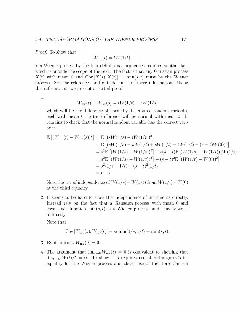
5.4. TRANSFORMATIONS OF THE WIENER PROCESS 177
Proof. To show thatWinv(t) = tW (1/t)
is a Wiener process by the four definitional properties requires another factwhich is outside the scope of the text. The fact is that any Gaussian processX(t) with mean 0 and Cov [X(s), X(t)] = min(s, t) must be the Wienerprocess. See the references and outside links for more information. Usingthis information, we present a partial proof:
1.Winv(t)−Winv(s) = tW (1/t)− sW (1/s)
which will be the difference of normally distributed random variableseach with mean 0, so the difference will be normal with mean 0. Itremains to check that the normal random variable has the correct vari-ance.
E[(Winv(t)−Winv(s))2
]= E
[(sW (1/s)− tW (1/t))2
]= E
[(sW (1/s)− sW (1/t) + sW (1/t)− tW (1/t)− (s− t)W (0))2
]= s2E
[(W (1/s)−W (1/t))2
]+ s(s− t)E [(W (1/s)−W (1/t))(W (1/t)−W (0))] + (s− t)2E
[(W (1/t)−W (0))2
]= s2E
[(W (1/s)−W (1/t))2
]+ (s− t)2E
[(W (1/t)−W (0))2
]= s2(1/s− 1/t) + (s− t)2(1/t)
= t− s
Note the use of independence of W (1/s)−W (1/t) from W (1/t)−W (0)at the third equality.
2. It seems to be hard to show the independence of increments directly.Instead rely on the fact that a Gaussian process with mean 0 andcovariance function min(s, t) is a Wiener process, and thus prove itindirectly.
Note that
Cov [Winv(s),Winv(t)] = stmin(1/s, 1/t) = min(s, t).
3. By definition, Winv(0) = 0.
4. The argument that limt→0Winv(t) = 0 is equivalent to showing thatlimt→∞W (t)/t = 0. To show this requires use of Kolmogorov’s in-equality for the Wiener process and clever use of the Borel-Cantelli

178 CHAPTER 5. BROWNIAN MOTION
lemma and is beyond the scope of this course. Use the translationproperty in the third statement of this theorem to prove continuity atevery value of t.
The following comments are adapted from Stochastic Calculus and Fi-nancial Applications by J. Michael Steele. Springer, New York, 2001, page40. These laws tie the Wiener process to three important groups of transfor-mations on [0,∞), and a basic lesson from the theory of differential equationsis that such symmetries can be extremely useful. On a second level, thelaws also capture the somewhat magical fractal nature of the Wiener pro-cess. The scaling law tells us that if we had even one-billionth of a second ofa Wiener process path, we could expand it to a billions years’ worth of anequally valid Wiener process path! The translation symmetry is not quite sostartling, it merely says that Wiener process can be restarted anywhere, thatis any part of a Wiener process captures the same behavior as at the origin.The inversion law is perhaps most impressive, it tells us that the first secondof the life of a Wiener process path is rich enough to capture the behavior ofa Wiener process path from the end of the first second until the end of time.
Sources
This section is adapted from: A First Course in Stochastic Processes by S.Karlin, and H. Taylor, Academic Press, 1975, pages 351–353 and FinancialDerivatives in Theory and Practice by P. J. Hunt and J. E. Kennedy, JohnWiley and Sons, 2000, pages 23–24.
Problems to Work for Understanding
1. Show that stmin(1/s, 1/t) = min(s, t)
2.
Outside Readings and Links:
1. Russell Gerrard, City University, London, Stochastic Modeling Notesfor the MSc in Actuarial Science, 2003-2004. Contributed by S. DunbarOctober 30, 2005.
5.5. HITTING TIMES AND RUIN PROBABILITIES 179
2. Yuval Peres, University of California Berkeley, Department of Statis-tics Notes on sample paths of Brownian Motion. Contributed by S.Dunbar, October 30, 2005.
5.5 Hitting Times and Ruin Probabilities
Rating
Mathematically Mature: may contain mathematics beyond calculus withproofs.
Section Starter Question
What is the probability that a simple random walk with p = 1/2 = q startingat the origin will hit value a > 0 before it hits value −b < 0, where b > 0?What do you expect in analogy for the standard Wiener process and why?
Key Concepts
1. With the Reflection Principle, we can derive the p.d.f of the hittingtime Ta.
2. With the hitting time, we can derive the c.d.f. of the maximum of theWiener Process on the interval 0 ≤ u ≤ t.
Vocabulary
1. The Reflection Principle for the Wiener process reflected about afirst passage has the same distribution as the original motion.
2. The hitting time Ta is the first time the Wiener process assumes thevalue a. Specifically in notation from analysis
Ta = inft > 0 : W (t) = a.

180 CHAPTER 5. BROWNIAN MOTION
Mathematical Ideas
Hitting Times
Consider the standard Wiener process W (t), which starts at W (0) = 0. Leta > 0. Let us denote the hitting time Ta be the first time the Wiener processhits a. Specifically in notation from analysis
Ta = inft > 0 : W (t) = a.
Note the very strong analogy with the duration of the game in the gambler’sruin.
Some Wiener process sample paths will hit a > 0 fairly directly. Otherswill make an excursion (for example, to negative values) and take a longtime to finally reach a. Thus Ta will have a probability distribution. We willdetermine that distribution by a heuristic procedure similar to the first stepanalysis we made for coin-flipping fortunes.
Specifically, we will consider a probability by conditioning, that is, con-ditioning on whether or not Ta ≤ t, for some given value of t.
P [W (t) ≥ a] = P [W (t) ≥ a|Ta ≤ t] P [Ta ≤ t]+P [W (t) ≥ a|Ta > t] P [Ta > t]
Now note that the second conditional probability is 0 because it is an emptyevent. Therefore:
P [W (t) ≥ a] = P [W (t) ≥ a|Ta ≤ t] P [Ta ≤ t] .
Now, consider Wiener process “started over” again the time Ta when it hitsa. By the shifting transformation from the previous section, this would havethe distribution of Wiener process again, and so
P [W (t) ≥ a|Ta ≤ t] = P [W (t) ≥ a|W (Ta) = a, Ta ≤ t]
= P [W (t)−W (Ta) ≥ 0|Ta ≤ t]
= 1/2.
This argument is a specific example of the Reflection Principle for the Wienerprocess. It says that the Wiener process reflected about a first passage hasthe same distribution as the original motion.
Actually, this argument contains a serious logical gap, since Ta is a randomtime, not a fixed time. That is, the value of Ta is different for each sample
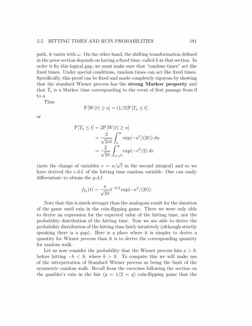
5.5. HITTING TIMES AND RUIN PROBABILITIES 181
path, it varies with ω. On the other hand, the shifting transformation definedin the prior section depends on having a fixed time, called h in that section. Inorder ti fix this logical gap, we must make sure that “random times” act likefixed times. Under special conditions, random times can act like fixed times.Specifically, this proof can be fixed and made completely rigorous by showingthat the standard Wiener process has the strong Markov property andthat Ta is a Markov time corresponding to the event of first passage from 0to a.
ThusP [W (t) ≥ a] = (1/2)P [Ta ≤ t] .
or
P [Ta ≤ t] = 2P [W (t) ≥ a]
=2√2πt
∫ ∞a
exp(−u2/(2t)) du
=2√2π
∫ ∞a/√t
exp(−v2/2) dv
(note the change of variables v = u/√t in the second integral) and so we
have derived the c.d.f. of the hitting time random variable. One can easilydifferentiate to obtain the p.d.f
fTa(t) =a√2πt−3/2 exp(−a2/(2t)).
Note that this is much stronger than the analogous result for the durationof the game until ruin in the coin-flipping game. There we were only ableto derive an expression for the expected value of the hitting time, not theprobability distribution of the hitting time. Now we are able to derive theprobability distribution of the hitting time fairly intuitively (although strictlyspeaking there is a gap). Here is a place where it is simpler to derive aquantity for Wiener process than it is to derive the corresponding quantityfor random walk.
Let us now consider the probability that the Wiener process hits a > 0,before hitting −b < 0, where b > 0. To compute this we will make useof the interpretation of Standard Wiener process as being the limit of thesymmetric random walk. Recall from the exercises following the section onthe gambler’s ruin in the fair (p = 1/2 = q) coin-flipping game that the

182 CHAPTER 5. BROWNIAN MOTION
probability that the random walk goes up to value a before going down tovalue b when the step size is ∆x is
P [ to a before −b ] =b∆x
(a+ b)∆x=
b
a+ b
Thus, the probability of a > 0, before hitting −b < 0 does not depend onthe step size, and also does not depend on the time interval. Therefore inpassing to the limit the probabilities should remain the same. Here is a placewhere it is easier to derive the result from the coin-flipping game and pass tothe limit than to derive the result directly from Wiener process principles.
The Distribution of the Maximum
Let t be a given time, let a > 0 be a given value, then
P[
max0≤u≤t
W (u) ≥ a
]= P [Ta ≤ t]
=2√2π
∫ ∞a/√t
exp(−y2/2) dy
Sources
This section is adapted from: Probability Models, by S. Ross, and A FirstCourse in Stochastic Processes Second Edition by S. Karlin, and H. Taylor,Academic Press, 1975.
Problems to Work for Understanding
1. Differentiate the c.d.f. of Ta to obtain the expression for the p.d.f of Ta.
2. Show that E [Ta] =∞ for a > 0.
3. Suppose that the fluctuations of a share of stock of a certain companyare well described by a Wiener process. Suppose that the companyis bankrupt if ever the share price drops to zero. If the starting shareprice is A(0) = 5, what is the probability that the company is bankruptby t = 25? What is the probability that the share price is above 10 att = 25?.
5.6. PATH PROPERTIES OF BROWNIAN MOTION 183
4. Suppose you own one share of stock whose price changes according to aWiener process. Suppose you purchased the stock at a price b+c, c > 0and the present price is b. You have decided to sell the stock eitherwhen it reaches the price b + c or when an additional time t goes by,whichever comes first. What is the probability that you do not recoveryour purchase price?
Outside Readings and Links:
1. Russell Gerrard, City University, London, Stochastic Modeling Notesfor the MSc in Actuarial Science, 2003-2004. Contributed by S. DunbarOctober 30, 2005.
2. Yuval Peres, University of California Berkeley, Department of Statis-tics Notes on sample paths of Brownian Motion. Contributed by S.Dunbar, October 30, 2005.
5.6 Path Properties of Brownian Motion
Rating
Mathematically Mature: may contain mathematics beyond calculus withproofs.
Section Starter Question
Provide an example of a continuous function which is not differentiable atsome point. Why does the function fail to have a derivative at that point?What are the possible reasons that a derivative could fail to exist at somepoint?
Key Concepts
1. With probability 1 a Brownian Motion path is continuous but nowheredifferentiable.
184 CHAPTER 5. BROWNIAN MOTION
Vocabulary
1. In probability theory, the term almost surely is used to indicate anevent which occurs with probability 1. In infinite sample spaces, it ispossible to have meaningful events with probability zero. So to say anevent occurs “almost surely” is not an empty phrase. Events occurringwith probability zero are sometimes called negligible events.
Mathematical Ideas
Properties of the Path of Brownian Motion
Theorem 17. With probability 1 (i.e. almost surely) Brownian Motion pathsare continuous functions.
To state this as a theorem may seem strange in view of property 4 of thedefinition of Brownian motion. Property 4 requires that Brownian motion iscontinuous. However, some authors weaken property 4 in the definition toonly require that Brownian motion be continuous at t = 0. Then this theoremshows that the weaker definition implies the stronger definition used in thistext. This theorem is difficult to prove, and well beyond the scope of thiscourse. In fact, even the statement above is imprecise. Specifically, there isan explicit representation of the defining properties of Brownian Motion asa function in which (with probability 1) W (t, ω) is a continuous function oft. We need the continuity for much of what we do later, and so this theoremis stated here again as a fact without proof.
Theorem 18. With probability 1 (i.e. almost surely) a Brownian Motion isnowhere (except possibly on set of Lebesgue measure 0) differentiable.
This property is even deeper and requires more machinery to prove thandoes the continuity theorem, so we will not prove it here. Rather, we use thisfact as another piece of evidence of the strangeness of Brownian Motion.
In spite of one’s intuition from calculus, Theorem 18 shows that contin-uous, nowhere differentiable functions are actually common. Indeed, con-tinuous, nowhere differentiable functions are useful for stochastic processes.One can imagine non-differentiability by considering the function f(t) = |t|which is continuous but not differentiable at t = 0. Because of the corner att = 0, the left and right limits of the difference quotient exist but are not
5.6. PATH PROPERTIES OF BROWNIAN MOTION 185
equal. Even more to the point, the function t2/3 is continuous but not differ-entiable at t = 0 because of a sharp “cusp” there. The left and right limitsof the difference quotient do not exist (more precisely, they approach ±∞)at x = 0. One can imagine Brownian Motion as being spiky with tiny cuspsand corners at every point. This becomes somewhat easier to imagine bythinking of the limiting approximation of Brownian Motion by coin-flippingfortunes. The re-scaled coin-flipping fortune graphs look spiky with cornerseverywhere. The approximating graphs suggest why the theorem is true,although this is not sufficient for the proof.
Theorem 19. With probability 1 (i.e. almost surely) a Brownian Motionpath has no intervals of monotonicity. That is, there is no interval [a, b] withW (t2)−W (t1) > 0 (or W (t2)−W (t1) < 0) for all t2, t1 ∈ [a, b] with t2 > t1
Theorem 20. With probability 1 (i.e. almost surely) Brownian Motion W (t)has
lim supn→∞
W (n)√n
= +∞,
lim infn→∞
W (n)√n
= −∞.
From Theorem 20 and the continuity we can deduce that for arbitrarilylarge t1, there is a t2 > t1 such that W (t2) = 0. That is, Brownian Motionpaths cross the time-axis at some time greater than any arbitrarily largevalue of t.
Theorem 21. With probability 1 (i.e. almost surely), 0 is an accumulationpoint of the zeros of W (t).
From Theorem 20 and the inversion tW (1/t) also being a standard Brow-nian motion, we deduce that 0 is an accumulation point of the zeros of W (t).That is, Standard Brownian Motion crosses the time axis arbitrarily near 0.
Theorem 22. With probability 1 (i.e. almost surely) the zero set of BrownianMotion
t ∈ [0,∞) : W (t) = 0is an uncountable closed set with no isolated points.

186 CHAPTER 5. BROWNIAN MOTION
Theorem 23. With probability 1 (i.e. almost surely) the graph of a BrownianMotion path has Hausdorff dimension 3/2.
This means that the graph of a Brownian Motion path is “fuzzier” or“thicker” than the graph of, for example, a continuously differentiable func-tion which would have Hausdorff dimension 1.
Sources
This section is adapted from: Notes on Brownian Motion by Yuval Peres,University of California Berkeley, Department of Statistics.
Problems to Work for Understanding
1. Provide a more complete heuristic argument based on Theorem 20 thatalmost surely there is a sequence tn with limt→∞ tn = ∞ such thatW (t) = 0
2. Provide a heuristic argument based on Theorem 21 and the shiftingproperty that the zero set of Brownian Motion
t ∈ [0,∞) : W (t) = 0
has no isolated points.
3. Looking in more advanced references, find another property of Brown-ian Motion which illustrates strange path properties.
Outside Readings and Links:
1. Notes on Brownian Motion Yuval Peres, University of California Berke-ley, Department of Statistics
5.7 Quadratic Variation of the Wiener Pro-
cess
Rating
Mathematically Mature: may contain mathematics beyond calculus withproofs.

5.7. QUADRATIC VARIATION OF THE WIENER PROCESS 187
Section Starter Question
What is an example of a function that “varies a lot”? What is an example of afunction that does not “vary a lot”? How would you measure the “variation”of a function?
Key Concepts
1. The total quadratic variation of Brownian motion is t.
2. This fact has profound consequences for dealing with Brownian motionanalytically and ultimately will lead to Ito’s formula.
Vocabulary
1. A function f(t) is said to have bounded variation if, over the closedinterval [a, b], there exists an M such that
|f(t1)− f(a)|+ |f(t2)− f(t1)|+ · · ·+ |f(b)− f(tn)| ≤M
for all partitions a = t0 < t1 < t2 < . . . < tn < tn+1 = b of the interval.
2. A function f(t) is said to have quadratic variation if, over the closedinterval [a, b], there exists an M such that
(f(t1)− f(a))2 + (f(t2)− f(t1))2 + · · ·+ (f(b)− f(tn))2 ≤M
for all partitions a = t0 < t1 < t2 < . . . < tn < tn+1 = b of the interval.
3. The mesh size of a partition P with a = t0 < t1 < . . . < tn < tn+1 = bis maxj=0,...,ntj+1 − tj|j = 1, . . . , n.
4. The total quadratic variation of a function f on an interval [a, b] is
supP
n∑j=0
(f(tj+1)− f(tj))2
where the supremum is taken over all partitions P with a = t0 < t1 <. . . < tn < tn+1 = b, with mesh size going to zero as the number ofpartition points n goes to infinity.
188 CHAPTER 5. BROWNIAN MOTION
Mathematical Ideas
Variation
Definition. A function f(x) is said to have bounded variation if, over theclosed interval [a, b], there exists an M such that
|f(t1)− f(a)|+ |f(t2)− f(t1)|+ · · ·+ |f(b)− f(tn)| ≤M
for all partitions a = t0 < t1 < t2 < . . . < tn < tn+1 = b of the interval.
The idea is that we measure the total (hence the absolute value) up-and-down movement of a function. This definition is similar to other partitionbased definitions such as the Riemann integral and the arclength of the graphof the function. A monotone increasing or decreasing function has boundedvariation. A function with a continuous derivative has bounded variation.Some functions, for instance Brownian Motion, do not have bounded varia-tion.
Definition. A function f(t) is said to have quadratic variation if, over theclosed interval [a, b], there exists an M such that
(f(t1)− f(a))2 + (f(t2)− f(t1))2 + · · ·+ (f(b)− f(tn))2 ≤M
for all partitions a = t0 < t1 < t2 < . . . < tn < tn+1 = b of the interval.
Again, the idea is that we measure the total (hence the positive termscreated by squaring) up-and-down movement of a function. However, thesquaring will make small ups-and-downs smaller, so that perhaps a functionwithout bounded variation may have quadratic variation. In fact, this is thecase for the Wiener Process.
Definition. The total quadratic variation of Q of a function f on aninterval [a, b] is
Q = supP
n∑i=0
(f(ti+1)− f(ti))2
where the supremum is taken over all partitions P with a = t0 < t1 < . . . <tn < tn+1 = b, with mesh size going to zero as the number of partition pointsn goes to infinity.

5.7. QUADRATIC VARIATION OF THE WIENER PROCESS 189
Quadratic Variation of the Wiener Process
We can guess that the Wiener Process might have quadratic variation byconsidering the quadratic variation of our coin-flipping fortune record first.Consider the function piecewise linear function W (t) defined by the sequenceof sums Tn = Y1 + · · ·+Yn from the Bernoulli random variables Yi = +1 withprobability p = 1/2 and Yi = −1 with probability q = 1−p = 1/2. With someanalysis, it is possible to show that we need only consider the quadratic vari-ation at points 1, 2, 3, . . . , n Then each term (W (i+ 1)− W (i))2 = Y 2
i+1 = 1.Therefore, the quadratic variation is the total number of steps, Q = n. Nowremember the Wiener Process is approximated by Wn(t) = (1/
√n)W (nt).
Each step is size 1/√n, then the quadratic variation of the step is 1/n
and there are n steps on [0, 1]. The total quadratic variation of Wn(t) =(1/√n)W (nt) on [0, 1] is 1.
We will not completely rigorously prove that the total quadratic variationof the Wiener Process is t, as claimed, but we will prove a theorem close tothe general definition of quadratic variation.
Theorem 24. Let W (t) be standard Brownian motion. For every fixed t > 0
limn→∞
2n∑n=1
[W
(k
2nt
)−W
(k − 1
2nt
)]2
= t
with probability 1 (that is, almost surely).
Proof. Introduce some briefer notation for the proof, let:
∆nk = W
(k
2nt
)−W
(k − 1
2nt
)k = 1, . . . , 2n
and
Wnk = ∆2nk − t/2n k = 1, . . . , 2n.
We want to show that∑2n
k=1 ∆2nk → t or equivalently:
∑2n
k=1Wnk → 0.For each n, the random variables Wnk, k = 1, . . . , 2n are independent andidentically distributed by properties 1 and 2 of the definition of standardBrownian motion. Furthermore,
E [Wnk] = E[∆2nk
]− t/2n = 0
190 CHAPTER 5. BROWNIAN MOTION
by property 1 of the definition of standard Brownian motion.A routine (but omitted) computation of the fourth moment of the normal
distribution shows that
E[W 2nk
]= 2t2/4n.
Finally, by property 2 of the definition of standard Brownian motion
E [WnkWnj] = 0, k 6= j.
Now, expanding the square of the sum, and applying all of these computa-tions
E
2n∑k=1
Wnk
2 =
2n∑k=1
E[W 2nk
]= 2n+1t2/4n = 2t2/2n.
Now apply Chebyshev’s Inequality to see:
P
[∣∣∣∣∣2n∑k=1
Wnk
∣∣∣∣∣ > ε
]≤ 2t2
ε2
(1
2
)n.
Now since∑
(1/2)n is a convergent series, the Borel-Cantelli lemma impliesthat the event ∣∣∣∣∣
2n∑k=1
Wnk
∣∣∣∣∣ > ε
can occur for only finitely many n. That is, for any ε > 0, there is an N ,such that for n > N ∣∣∣∣∣
2n∑k=1
Wnk
∣∣∣∣∣ < ε.
Therefore we must have that limn→∞∑2n
k=1Wnk = 0, and we have establishedwhat we wished to show.
Remark. Here’s a less rigorous and somewhat different explanation of whythe squared variation of Brownian motion may be guessed to be t, see [5].Consider
n∑k=1
(W
(kt
n
)−W
((k − 1)t
n
))2
.
5.7. QUADRATIC VARIATION OF THE WIENER PROCESS 191
Now let
Znk =
(W(ktn
)−W
((k−1)tn
))√t/n
Then for each n, the sequence Znk is a sequence of independent, identicallydistributed standard normal N(0, 1) random variables. Now we can writethe quadratic variation as:
n∑k=1
∆2nk =
n∑k=1
t
nZ2nk = t
(1
n
n∑k=1
Z2nk
)
But notice that the expectation E(Z2nk) of each term is the same as calcu-
lating the variance of a standard normal N(0, 1) which is of course 1. Thenthe last term in parentheses above converges by the weak law of large num-bers to 1! Therefore the quadratic variation of Brownian motion convergesto t. This little proof is in itself not sufficient to prove the theorem abovebecause it relies on the weak law of large of numbers. Hence the theoremestablishes convergence in distribution only while for the theorem above wewant convergence almost surely.
Remark. Starting from
limn→∞
2n∑n=1
[W
(k
2nt
)−W
(k − 1
2nt
)]2
= t
and without thinking too carefully about what it might mean, we can imaginean elementary calculus limit to the left side and write the formula:∫ t
0
[dW (τ)]2 = t =
∫ t
0
dτ.
In fact, with more advanced mathematics this can be made sensible ad math-ematically sound. Now from this relation, we could write the integral equalityin differential form:
dW (τ)2 = dτ.
The important thing to remember here is that the formula suggests thatBrownian motion has differentials that cannot be ignored in second (orsquared, or quadratic) order. Brownian motion “wiggles” so much that eventhe total of the squared differences add up! In retrospect, this is not so
192 CHAPTER 5. BROWNIAN MOTION
surprising given the law of the iterated logarithm. We know that in anyneighborhood [t, t + dt] to the right of t, Brownian motion must come closeto√
2t log log t. That is, intuitively, W (t + dt) −W (t) must be about√
2dtin magnitude, so we would guess dW 2 ≈ 2dt The theorem makes it precise.
Remark. This theorem can be nicely summarized in the following way: LetdW (t) = W (t + dt) − W (t). Let dW (t)2 = (W (t + dt) − W (t))2. Then(although mathematically not rigorously) we can say:
dW (t) ∼ N(0, dt)
(dW (t))2 ∼ N(dt, 0).
Theorem 25.
limn→∞
2n∑n=1
∣∣∣∣W (k
2nt
)−W
(k − 1
2nt
)∣∣∣∣ =∞
In other words, the total variation of a Brownian path is infinite, with prob-ability 1.
Proof.
2n∑n=1
∣∣∣∣W (k
2nt
)−W
(k − 1
2nt
)∣∣∣∣ ≥ ∑2n
n=1
∣∣W (k2n t)−W
(k−12n t)∣∣2
maxj=1,...,2n
∣∣W (k2n t)−W
(k−12n t)∣∣
The numerator on the right converges to t, while the denominator goes to 0because Brownian paths are continuous, therefore uniformly continuous onbounded intervals. Therefore the faction on the right goes to infinity.
Sources
The theorem in this section is drawn from A First Course in StochasticProcesses by S. Karlin, and H. Taylor, Academic Press, 1975. The heuristicproof using the weak law was taken from Financial Calculus: An introductionto derivative pricing by M Baxter, and A. Rennie, Cambridge UniversityPress, 1996, page 59. The mnemonic statement of the quadratic variation indifferential form is derived from Steele’s text.

5.7. QUADRATIC VARIATION OF THE WIENER PROCESS 193
Problems to Work for Understanding
1. Show that a monotone increasing function has bounded variation.
2. Show that a function with continuous derivative has bounded variation.
3. Show that the function
f(t) =
t2 sin(1/t) 0 < t ≤ 1
0 t = 0
is of bounded variation, while the function
f(t) =
t sin(1/t) 0 < t ≤ 1
0 t = 0
is not of bounded variation.
4. Show that a continuous function of bounded variation is also of quadraticvariation.
5. Show that the fourth moment E [Z4] = 3 where Z ∼ N(0, 1). Thenshow that
E[W 2nk
]= 2t2/4n
Outside Readings and Links:
1. Yuval Peres, University of California Berkeley, Department of StatisticsNotes on sample paths of Brownian Motion. Contributed by S. Dunbar,October 30, 2005.
2. Wikipedia, Quadratic variation Contributed by S. Dunbar, November10, 2009.
3. Michael Kozdron, University of Regina, Contributed by S. Dunbar,November 10, 2009.

194 CHAPTER 5. BROWNIAN MOTION

Chapter 6
Stochastic Calculus
6.1 Stochastic Differential Equations and the
Euler-Maruyama Method
Rating
Mathematically Mature: may contain mathematics beyond calculus withproofs.
Section Starter Question
Explain how to use a slope-field diagram to solve the ordinary differentialequation
dx
dt= x.
Key Concepts
1. We can numerically simulate the solution to stochastic differential equa-tions with an analog to Euler’s method, called the Euler-Maruyama(EM) method.
Vocabulary
1. A stochastic differential equation is a mathematical equation relat-ing a stochastic process to its local deterministic and random compo-
195

196 CHAPTER 6. STOCHASTIC CALCULUS
nents. The goal is to unravel the relation to find the stochastic process.Under mild conditions on the relationship, and with a specifying initialcondition, solutions of stochastic differential equations exist and areunique.
2. The Euler-Maruyama (EM) method is a numerical method forsimulating the solutions of a stochastic differential equation based onthe definition of the Ito stochastic integral: Given
dX(t) = G(X(t))dt+H(X(t))dW (t), X(t0) = X0,
and a step size dt, we approximate and simulate with
Xj = Xj−1 +G(Xj−1)dt+H(Xj−1)(W (tj−1 + dt)−W (tj−1))
3. Extensions and variants of Standard Brownian Motion defined throughstochastic differential equations are Brownian Motion with drift,scaled Brownian Motion, and geometric Brownian Motion.
Mathematical Ideas
Stochastic Differential Equations: Symbolically
The straight line segment is the building block of differential calculus. Thebasic idea behind differential calculus is that differentiable functions, no mat-ter how difficult their global behavior, are locally approximated by straightline segments. In particular, this is the idea behind Euler’s method for ap-proximating differentiable functions defined by differential equations.
We know that rescaling (“zooming in” on) Brownian motion does notproduce a straight line, it produces another image of Brownian motion. Thisself-similarity is ideal for an infinitesimal building block, for instance, wecould build global Brownian motion out of lots of local “chunks” of Brow-nian motion. This suggests we could build other stochastic processes outof suitably scaled Brownian motion. In addition, if we include straight linesegments we can overlay the behavior of differentiable functions onto thestochastic processes as well. Thus, straight line segments and “chunks” ofBrownian motion are the building blocks of stochastic calculus.
With stochastic differential calculus, we can build a nice class of newstochastic processes. We do this by specifying how to build the new stochastic

6.1. STOCHASTIC DIFFERENTIAL EQUATIONS AND THE EULER-MARUYAMA METHOD197
processes locally from our base deterministic function, the straight line andour base stochastic process, Standard Brownian Motion. We write the localchange in value of the stochastic process over a time interval of (infinitesimal)length dt as
dX = G(X(t)) dt+H(X(t)) dW (t), X(t0) = X0.
Note that we are not allowed to write
dX
dt= G(X(t)) +H(X(t))
dW
dt,X(t0) = X0
since Standard Brownian Motion is nowhere differentiable with probability1. (Actually, the informal stochastic differential equation is a compact way ofwriting a rigorously defined, equivalent implicit Ito integral equation. Sincewe do not have the required rigor, we will approach the stochastic differentialequation intuitively.)
The stochastic differential equation says the initial point (t0, X0) is spec-ified, perhaps with X0 a random variable with a given distribution. A deter-ministic component at each point has a slope determined through G at thatpoint. In addition, there is some random perturbation that effects the evolu-tion of the process. The variance of the random perturbation is determined ateach point through the function H. This is a simple expression of a StochasticDifferential Equation (SDE) which determines a stochastic process, just as anOrdinary Differential Equation (ODE) determines a differentiable function.We infinitesimally extend the process with the incremental change informa-tion and repeat. This is an expression in words of the Euler-Maruyamamethod for numerically simulating the stochastic differential expression.
Example. The simplest stochastic differential equation is
dX = r dt+ dW, X(0) = b
where r is a constant. Take a deterministic initial condition to be X(0) = b.This process is the stochastic extension of the differential equation expressionof a straight line. The new stochastic process X is drifting or trending at rater with a random variation due to Brownian Motion perturbations aroundthat trend. We will later show explicitly that the solution of this SDE isX(t) = b + rt + W (t) although it is seems intuitively clear that this shouldbe the process. We will call this Brownian motion with drift.

198 CHAPTER 6. STOCHASTIC CALCULUS
Example. The next simplest stochastic differential equation is
dX = σdW, X(0) = b
This stochastic differential equation says that the process is evolving as a mul-tiple of Standard Brownian Motion. The solution may be easily guessed asX(t) = σW (t) which has variance σ2t on increments of length t. Sometimesthis is called Brownian Motion (in contrast to Standard Brownian Motionwhich has variance t on increments of length t).
We can combine the previous two examples to consider
dX = rdt+ σdW, X(0) = b
which would have solution X(t) = b+ rt+σW (t), a multiple of BrownianMotion with drift r started at b. Sometimes this extension of StandardBrownian motion is called Brownian Motion. Some authors consider thisprocess directly instead of the more special case we considered in the previouschapter.
Example. The next simplest and first non-trivial differential equation is dX =X dW . Here the differential equation says that process is evolving like Brow-nian motion with a variance which is the same as the process value. When theprocess is small, the variance is small, when the process is large, the varianceis large. Expressing the stochastic differential equation as dX/X = dW wemay say that the relative change acts like Standard Brownian Motion. Theresulting stochastic process is called geometric Brownian motion and itwill figure extensively in what we consider later as models of security prices.
Example. The next simplest differential equation is
dX = rX dt+ σX dW, X(0) = b.
Here the stochastic differential equation says that the growth of the processat a point is proportional to the process value, with a random perturbationproportional to the process value. Again looking ahead, we could write thedifferential equation as dX/X = rdt+σdW and interpret it to say the relativerate of increase is proportional to the time observed together with a randomperturbation like a Brownian segment proportional to the length of time.

6.1. STOCHASTIC DIFFERENTIAL EQUATIONS AND THE EULER-MARUYAMA METHOD199
Stochastic Differential Equations: Numerically
The sample path that the Euler-Maruyama method produces numerically isthe analog of using the Euler method.
The formula for the Euler-Maruyama (EM) method is based on the defi-nition of the Ito stochastic integral:
Xj = Xj−1+G(Xj−1)dt+H(Xj−1)(W (tj−1+dt))−W (tj−1), tj = tj−1+dt.
Note that the initial conditions X0 and t0 set the starting point.We do not use Brownian motion directly to obtain the incrementsW (tj−1+
dt)−W (tj−1) since we don’t have a direct source of values of Brownian Mo-tion. Instead we use coin-flipping sequences of an appropriate length tocreate an approximation to W (t). Note that since the increments W (tj−1 +dt) −W (tj−1) are independent and identically distributed, we will be ableto use independent coin-flip sequences to generate the approximation of theincrements. For convenience, we generate the approximations using a ran-dom number generator, but we could as well use actual coin-flipping. Thegeneration of the sequences is not recorded, only the summed and scaled(independently sampled) outcomes for
W (dt) ≈ WN(dt) =W (N dt)√
N=√dtW (N dt)√
N dt.
For convenience, I will take dt = 1/10, N = 100, so we need W (100 ·(1/10))/
√100 = T10/10. Also, I will take r = 2, b = 1, and σ = 1, so
we simulate the solution of
dX = 2X dt+X dW, X(0) = 1.
j tj Xj 2Xj dt dW XjdW 2Xj +XjdW Xj + 2Xj dt+XjdW0 0 1 0.2 0 0 0.2 1.21 0.1 1.2 0.24 0.2 0.24 0.48 1.682 0.2 1.68 0.34 -0.2 -0.34 0.0 1.683 0.3 1.68 0.34 0.4 0.67 1.01 2.694 0.4 2.69 0.54 -0.2 -0.54 0.0 2.695 0.5 2.69 0.54 0 0 0.54 3.236 0.6 3.23 0.65 0.4 1.29 1.94 5.167 0.7 5.16 1.03 0.4 2.06 3.1 8.268 0.8 8.26 1.65 0.4 3.3 4.95 13.219 0.9 13.21 2.64 0 0 2.64 15.8510 1.0 15.85
200 CHAPTER 6. STOCHASTIC CALCULUS
Of course, this can be programmed and the step size made much smaller,presumably with better approximation properties. In fact, it is possible toconsider kinds of convergence for the EM method comparable to the StrongLaw of Large Numbers and the Weak Law of Large Numbers.
Sources
This section is adapted from: “An Algorithmic Introduction to the NumericalSimulation of Stochastic Differential Equations”, by Desmond J. Higham, inSIAM Review, Vol. 43, No. 3, pp. 525-546, 2001 and Financial Calculus: Anintroduction to derivative pricing by M Baxter, and A. Rennie, CambridgeUniversity Press, 1996, pages 52-62.
Problems to Work for Understanding
1. Simulate the solution of the stochastic differential equation
dX(t) = X(t)dt+ 2X(t)dX
on the interval [0, 1] with initial condition X(0) = 1 and step size∆t = 1/10.
2. Simulate the solution of the stochastic differential equation
dX(t) = tX(t)dt+ 2X(t)dX
on the interval [0, 1] with initial condition X(0) = 1 and step size∆t = 1/10. Note the difference with the previous problem, now themultiplier of the dt term is a function of time.
Outside Readings and Links:
1. Maple Stochastic Package The MAPLE stochastic package offers anumber of MAPLE routines for stochastic differential equations.
2. Matlab program files for Stochastic Differential Equations offers a num-ber of MATLAB routines for stochastic differential equations.
6.2. ITO’S FORMULA 201
6.2 Ito’s Formula
Rating
Mathematically Mature: may contain mathematics beyond calculus withproofs.
Section Starter Question
State the Taylor expansion of a function f(x) up to order 1. What is therelation of this expansion to the Mean Value Theorem of calculus? What isthe relation of this expansion to the Fundamental Theorem of calculus?
Key Concepts
1. Ito’s formula is an expansion expressing a stochastic process in terms ofthe deterministic differential and the Wiener process differential, thatis, the stochastic differential equation for the process.
2. Solving stochastic differential equations follows by guessing solutionsbased on comparison with the form of Ito’s formula.
Vocabulary
1. Ito’s formula is often also called Ito’s lemma by other authors andtexts. Some authors believe that this result is more important than amere lemma, and so I adopt the alternative name of “formula”. “For-mula” also emphasizes the analogy with the chain “rule” and the Taylor“expansion”.
Mathematical Ideas
Ito’s Formula and Ito calculus
We need some operational rules that allow us to manipulate stochastic pro-cesses with stochastic calculus.
The important thing to know about traditional differential calculus isthat it is the
• the Fundamental Theorem of Calculus,

202 CHAPTER 6. STOCHASTIC CALCULUS
• chain rule, and
• Taylor polynomials and Taylor series
that enable us to calculate with functions. A deeper understanding of calcu-lus recognizes that these three calculus theorems are all aspects of the samefundamental idea. Likewise we need similar rules and formulas for stochasticprocesses. Ito’s formula will perform that function for us. However, Ito’sformula acts in the capacity of all three of the calculus theorems, and wehave only one such theorem for stochastic calculus.
The next example will show us that we will need some new rules forstochastic calculus, the old rules from calculus will no longer make sense.
Example. Consider the process which is the square of the Wiener process:
Y (t) = W (t)2.
We notice that this process is always non-negative, Y (0) = 0, Y has infinitelymany zeroes on t > 0 and E [Y (t)] = E [W (t)2] = t. What more can we sayabout this process? For example, what is the stochastic differential of Y (t)and what would that tell us about Y (t)?
Using naive calculus, we might conjecture using the ordinary chain rule
dY = 2W (t)dW (t).
If that were true then the Fundamental Theorem of Calculus would imply
Y (t) =
∫ t
0
dY =
∫ t
0
2W (t) dW (t)
should also be true. But consider∫ t
02W (t) dW (t). It ought to correspond to
a limit of a summation (for instance a Riemann-Stieltjes left sum):∫ t
0
2W (t)dW (t) ≈n∑i=1
2W ((i− 1)t/n)[W (it/n)−W ((i−)t/n)]
But look at this carefully: W ((i − 1)t/n) = W ((i − 1)t/n) −W (0) is inde-pendent of [W (it/n) − W ((i−)t/n)] by property 2 of the definition of the

6.2. ITO’S FORMULA 203
Wiener process. Therefore, the expected value, or mean, of the summationwill be zero:
E [Y (t)] = E[∫ t
0
2W (t)dW (t)
]= E
[limn→∞
n∑i=1
2W ((i− 1)t/n)(W (it/n)−W ((i− 1)t/n))
]
= limn→∞
n∑i=1
2E [[W ((i− 1)t/n)−W (0)][W (it/n)−W ((i−)t/n)]]
= 0.
(Note the assumption that the limit and the expectation can be interchanged!)But the mean of Y (t) = W (t)2 is t which is definitely not zero! The
two stochastic processes don’t agree even in the mean, so something is notright! If we agree that the integral definition and limit processes should bepreserved, then the rules of calculus will have to change.
We can see how the rules of calculus must change by rearranging thesummation. Use the simple algebraic identity
2b(a− b) =(a2 − b2 − (a− b)2
)to re-write∫ t
0
2W (t)dW (t) = limn→∞
n∑i=1
2W ((i− 1)t/n)[W (it/n)−W ((i− 1)t/n)]
= limn→∞
n∑i=1
(W (it/n)2 −W ((i− 1)t/n)2 − (W (it/n)−W ((i− 1)t/n))
)2= lim
n→∞
(W (t)2 −W (0)2 −
n∑i=1
(W (it/n)−W ((i− 1)t/n))2
)
= W (t)2 − limn→∞
n∑i=1
(W (it/n)−W ((i− 1)t/n))2
We recognize the second term in the last expression as being the quadraticvariation of Wiener process, which we have already evaluated, and so∫ t
0
2W (t)dW (t) = W (t)2 − t.
204 CHAPTER 6. STOCHASTIC CALCULUS
Theorem 26 (Ito’s formula). If Y (t) is scaled Wiener process with drift,satisfying dY = r dt+σ dW and f is a twice continuously differentiable func-tion, then Z(t) = f(Y (t)) is also a stochastic process satisfying the stochasticdifferential equation
dZ = (rf ′(Y ) + (σ2/2)f ′′(Y )) dt+ (σf ′(Y )) dW.
In words, Ito’s formula in this form tells us how to expand (in analogywith the chain rule or Taylor’s formula) the differential of a process which isdefined as an elementary function of scaled Brownian motion with drift.
Example. Consider Z(t) = W (t)2. Here the stochastic process is standardBrownian Motion, so r = 0 and σ = 1 so dY = dW . The twice continuouslydifferentiable function f is the squaring function, f(x) = x2, f ′(x) = 2x andf ′′(x) = 2. Then according to Ito’s formula:
d(W 2) = (0 · (2W (t)) + (1/2)(2))dt+ (1 · 2W (t))dW = dt+ 2W (t)dW
Notice the additional dt term! Note also that if we repeated the integrationsteps above in the example, we would obtain W (t)2 as expected!
The case where dY = dW , that is the base process is Standard BrownianMotion so Z = f(W ), occurs commonly enough that we record Ito’s formulafor this special case:
Corollary 8 (Ito’s Formula applied to functions of standard Brownian Mo-tion). If f is a twice continuously differentiable function, then Z(t) = f(W (t))is also a stochastic process satisfying the stochastic differential equation
dZ = df(W ) = (1/2)f ′′(W ) dt+ f ′(W ) dW.
Example. Consider Geometric Brownian Motion
exp(rt+ σW (t)).
What SDE does Geometric Brownian Motion follow? Take Y (t) = rt +σW (t), so that dY = rdt+ σdW . Then Geometric Brownian Motion can bewritten as Z(t) = exp(Y (t)), so f is the exponential function. Ito’s formulais
dZ = (rf ′(Y (t)) + (1/2)σ2f ′′Y (t)) + σf ′(Y )dW
Computing the derivative of the exponential function and evaluating, f ′(Y (t)) =exp(Y (t)) = Z(t) and likewise for the second derivative. Hence
dZ = (r + (1/2)σ2)Z(t)dt+ σZ(t)dW
6.2. ITO’S FORMULA 205
Guessing Processes from SDEs with Ito’s Formula
One of the key needs we will have is to go in the opposite direction and con-vert SDEs to processes, in other words to solve SDEs. We take guidance fromordinary differential equations, where finding solutions to differential equa-tions comes from judicious guessing based on a through understanding andfamiliarity with the chain rule. For SDEs the solution depends on inspiredguesses based on a thorough understanding of the formulas of stochastic cal-culus. Following the guess we require a proof that the proposed solution isan actual solution, again using the formulas of stochastic calculus.
A few rare examples of SDEs can be solved with explicit familiar func-tions. This is just like ODEs in that the solutions of many simple differentialequations cannot be solved in terms of elementary functions. The solutionsof the differential equations define new functions which are useful in appli-cations. Likewise, the solution of an SDE gives us a way of defining newprocesses which are useful.
Example. Suppose we are asked to solve the SDE
dZ(t) = σZ(t)dW.
We need an inspired guess, so we try
exp(rt+ σW (t))
where r is a constant to be determined while the σ term is given in the SDE.Ito’s formula for the guess is
dZ = (r + (1/2)σ2)Z(t)dt+ σZ(t)dW.
We notice that the stochastic term (or Wiener process differential term) isthe same as the SDE. We need to choose the constant r appropriately in thedeterministic or drift differential term. If we choose r to be −(1/2)σ2 thenthe drift term in the differential equation would match the SDE we have tosolve as well. We therefore guess
Y (t) = exp(σW (t)− (1/2)σ2t).
We should double check by applying Ito’s formula.Solvable SDEs are scarce, and this one is special enough to give a name.
It is the Dolean’s exponential of Brownian motion.
206 CHAPTER 6. STOCHASTIC CALCULUS
Sources
This discussion is adapted from Financial Calculus: An introduction toderivative pricing by M Baxter, and A. Rennie, Cambridge University Press,1996, pages 52–62 and “An Algorithmic Introduction to the Numerical Sim-ulation of Stochastic Differential Equations”, by Desmond J. Higham, inSIAM Review, Vol. 43, No. 3, pages 525–546, 2001.
Problems to Work for Understanding
1. Find the solution of the stochastic differential equation
dY (t) = Y (t)dt+ 2Y (t)dW
2. Find the solution of the stochastic differential equation
dY (t) = tY (t)dt+ 2Y (t)dW
Note the difference with the previous problem, now the multiplier ofthe dt term is a function of time.
3. Find the solution of the stochastic differential equation
dY (t) = µY (t)dt+ σY (t)dW
4. Find the solution of the stochastic differential equation
dY (t) = µtY (t)dt+ σY (t)dW
Note the difference with the previous problem, now the multiplier ofthe dt term is a function of time.
5. Find the solution of the stochastic differential equation
dY (t) = µ(t)Y (t)dt+ σY (t)dX
Note the difference with the previous problem, now the multiplier of thedt term is a general (technically, a locally bounded integrable) functionof time.
6.3. PROPERTIES OF GEOMETRIC BROWNIAN MOTION 207
Outside Readings and Links:
1.
2.
3.
4.
6.3 Properties of Geometric Brownian Mo-
tion
Rating
Mathematically Mature: may contain mathematics beyond calculus withproofs.
Section Starter Question
For the ordinary differential equation
dx
dt= rx x(0) = x0
what is the rate of growth of the solution?
Key Concepts
1. Geometric Brownian Motion is the continuous time stochastic processz0 exp(µt+ σW (t)) where W (t) is standard Brownian Motion.
2. The mean of Geometric Brownian Motion is
z0 exp(µt+ (1/2)σ2t).
3. The variance of Geometric Brownian Motion is
z20 exp(2µt+ σ2t)(exp(σ2t)− 1).

208 CHAPTER 6. STOCHASTIC CALCULUS
Vocabulary
1. Geometric Brownian Motion is the continuous time stochastic pro-cess z0 exp(µt+ σW (t)) where W (t) is standard Brownian Motion.
2. A random variable X is said to have the lognormal distribution (withparameters µ and σ) if log(X) is normally distributed (log(X) ∼ N(µ, σ2)).The p.d.f. for X is
fX(x) =1√
2πσxexp((−1/2)[(ln(x)− µ)/σ]2).
Mathematical Ideas
Geometric Brownian Motion
Geometric Brownian Motion is the continuous time stochastic processX(t) = z0 exp(µt+ σW (t)) where W (t) is standard Brownian Motion. Mosteconomists prefer Geometric Brownian Motion as a model for market pricesbecause it is always positive, in contrast to Brownian Motion, even Brow-nian Motion with drift. Furthermore, as we have seen from the stochasticdifferential equation for Geometric Brownian Motion, the differential relativechange in Geometric Brownian Motion is a combination of a deterministicproportional growth term similar to inflation or interest rate growth plus arandom relative change. See Ito’s Formula and Stochastic Calculus. On ashort time scale this is a sensible economic model.
Theorem 3. At fixed time t, Geometric Brownian Motion z0 exp(µt+σW (t))has a lognormal distribution with parameters (ln(z0) + µt) and σ
√t.
Proof.
FX(x) = P [X ≤ x]
= P [z0 exp(µt+ σW (t)) ≤ x]
= P [µt+ σW (t) ≤ ln(x/z0)]
= P [W (t) ≤ (ln(x/z0)− µt)/σ]
= P[W (t)/
√t ≤ (ln(x/z0)− µt)/(σ
√t)]
=
∫ (ln(x/z0)−µt)/(σ√t)
−∞
1√2π
exp(−y2/2) dy

6.3. PROPERTIES OF GEOMETRIC BROWNIAN MOTION 209
Figure 6.1: The p.d.f. for a lognormal random variable
Now differentiating with respect to x, we obtain that
fX(x) =1√
2πσx√t
exp((−1/2)[(ln(x)− ln(z0)− µt)/(σ√t)]2).
Calculation of the Mean
We can calculate the mean of Geometric Brownian Motion by using the m.g.f.for the normal distribution.
Theorem 4. E [z0 exp(µt+ σW (t))] = z0 exp(µt+ (1/2)σ2t)
Proof.
E [X(t)] = E [z0 exp(µt+ σW (t))]
= z0 exp(µt)E [exp(σW (t))]
= z0 exp(µt)E [exp(σW (t)u)] |u=1
= z0 exp(µt) exp(σ2tu2/2)|u=1
= z0 exp(µt+ (1/2)σ2t)
since σW (t) ∼ N(0, σ2t) and E [exp(Y u)] = exp(σ2tu2/2) when Y ∼ N(0, σ2t).See Moment Generating Functions, Theorem 4.
210 CHAPTER 6. STOCHASTIC CALCULUS
Calculation of the Variance
We can calculate the variance of Geometric Brownian Motion by using them.g.f. for the normal distribution, together with the common formula
Var [X] = E[(X − E [X])2
]= E
[X2]− (E [X])2
and the previously obtained formula for E [X].
Theorem 5. Var [z0 exp(µt+ σW (t))] = z20 exp(2µt+ σ2t)[exp(σ2t)− 1]
Proof. First compute:
E[X(t)2
]= E
[z20 exp(µt+ σW (t))2
]= z2
0E [exp(2µt+ 2σW (t))]
= z20 exp(2µt)E [exp(2σW (t))]
= z20 exp(2µt)E [exp(2σW (t)u)] |u=1
= z20 exp(2µt) exp(4σ2tu2/2)|u=1
= z20 exp(2µt+ 2σ2t)
Therefore,
Var [z0 exp(µt+ σW (t))] = z20 exp(2µt+ 2σ2t)− z2
0 exp(2µt+ σ2t)
= z20 exp(2µt+ σ2t)[exp(σ2t)− 1].
Note that this has the consequence that the variance starts at 0 and thenincreases. The variation of Geometric Brownian Motion starts small, andthen increases, so that the motion generally makes larger and larger swingsas time increases.
Parameter Summary
If a Geometric Brownian Motion is defined by the stochastic differential equa-tion
dX = rXdt+ σXdW X(0) = z0
then the Geometric Brownian Motion is
X(t) = z0 exp((r − (1/2)σ2)t+ σW (t)).
6.3. PROPERTIES OF GEOMETRIC BROWNIAN MOTION 211
At each time the Geometric Brownian Motion has lognormal distributionwith parameters (ln(z0)+rt−(1/2)σ2t) and σ
√t. The mean of the Geometric
Brownian Motion is E [X(t)] = z0 exp(rt). The variance of the GeometricBrownian Motion is
Var [X(t)] = z20 exp(2rt)[exp(σ2t)− 1]
If the primary object is the Geometric Brownian Motion
X(t) = z0 exp(µt+ σW (t)).
then by Ito’s formula the SDE satisfied by this stochastic process is
dX = (µ+ (1/2)σ2)X(t)dt+ σX(t)dW X(0) = z0.
At each time the Geometric Brownian Motion has lognormal distributionwith parameters (ln(z0)+µt) and σ
√t. The mean of the Geometric Brownian
Motion is E [X(t)] = z0 exp(µt + (1/2)σ2t). The variance of the GeometricBrownian Motion is
z20 exp(2µt+ σ2t)[exp(σ2t)− 1].
Ruin and Victory Probabilities for Geometric Brownian Motion
Because of the exponential-logarithmic connection between Geometric Brow-nian Motion and Brownian Motion, many results for Brownian Motion canbe immediately translated into results for Geometric Brownian Motion. Hereis a result on the probability of victory, now interpreted as the condition ofreaching a certain multiple of the initial value. For A < 1 < B define the“duration to ruin or victory”, or the “hitting time” as
TA,B = mint ≥ 0 :z0 exp(µt+ σW (t))
z0
= A,z0 exp(µt+ σW (t))
z0
= B
Theorem 6. For a Geometric Brownian Motion with parameters µ and σ,and A < 1 < B,
P[z0 exp(µtA,B + σW (TA,B))
z0
= B
]=
1− A1−(2µ−σ2)/σ2
B1−(2µ−σ2)/σ2 − A1−(2µ−σ2)/σ2
212 CHAPTER 6. STOCHASTIC CALCULUS
Quadratic Variation of Geometric Brownian Motion
The quadratic variation of Geometric Brownian Motion may be deduced fromIto’s formula:
dX = (µ− σ2/2)Xdt+ σXdW
so that
(dX)2 = (µ− σ2/2)2X2dt2 + (µ− σ2/2)X2σdtdW + σ2X2(dW )2.
Operating on the principle that terms of order (dt)2 and dt ·dW are smalland may be ignored, and that (dW )2 = dt, we obtain:
(dX)2 = σ2X2dt.
Sources
This section is adapted from: A First Course in Stochastic Processes, SecondEdition, by S. Karlin and H. Taylor, Academic Press, 1975, page 357; AnIntroduction to Stochastic Modeling 3rd Edition, by H. Taylor, and S. Karlin,Academic Press, 1998, pages 514-516; and Introduction to Probability Models9th Edition, S. Ross, Academic Press, 2006.
Problems to Work for Understanding
1. Differentiate ∫ (ln(x/z0)−µt)/(σ√t)
−∞
1√2π
exp(−y2/2) dy
to obtain the p.d.f. of Geometric Brownian Motion.
2. What is the probability that Geometric Brownian Motion with param-eters µ = −σ2/2 and σ (so that the mean is constant) ever rises tomore than twice its original value? In economic terms, if you buy stockwhose fluctuations are described by Geometric Brownian Motion, whatare your chances to double your money?

6.3. PROPERTIES OF GEOMETRIC BROWNIAN MOTION 213
3. What is the probability that Geometric Brownian Motion with param-eters µ = 0 and σ ever rises to more than twice its original value? Ineconomic terms, if you buy stock whose fluctuations are described byGeometric Brownian Motion, what are your chances to double yourmoney?
4. Derive the probability of ruin (the probability of Geometric BrownianMotion hitting A < 1 before hitting B > 1).
Outside Readings and Links:
1.
2.
3.
4.

214 CHAPTER 6. STOCHASTIC CALCULUS
Chapter 7
The Black-Scholes Model
7.1 Derivation of the Black-Scholes Equation
Rating
Mathematically Mature: may contain mathematics beyond calculus withproofs.
Section Starter Question
What is the most important idea in the derivation of the binomial optionpricing model?
Key Concepts
1. The derivation of the Black-Scholes equation uses
(a) tools from calculus,
(b) the quadratic variation of Geometric Brownian Motion,
(c) the no-arbitrage condition to evaluate growth of non-risky portfo-lios,
(d) and a simple but profound insight to eliminate the randomness orrisk.
215

216 CHAPTER 7. THE BLACK-SCHOLES MODEL
Vocabulary
1. A backward parabolic PDE is a partial differential equation of theform Vt + DVxx + . . . = 0 with highest derivative terms in t of order1 and highest derivative terms x of order 2 respectively. Terminalvalues V (S, T ) at an end time t = T must be satisfied in contrast tothe initial values at t = 0 required by many problems in physics andengineering.
2. A terminal condition for a backward parabolic equation is the speci-fication of a function at the end time of the interval of consideration touniquely determine the solution. It is analogous to an initial conditionfor an ordinary differential equation, except that it occurs at the endof the time interval, instead of the beginning.
Mathematical Ideas
Explicit Assumptions Made for Modeling and Derivation
For mathematical modeling of a market for a risky security we will ideallyassume
1. that a large number of identical, rational traders always have completeinformation about all assets they are trading,
2. changes in prices are given by a continuous random variable with someprobability distribution,
3. that trading transactions take negligible time,
4. purchases and sales can be made in any amounts, that is, the stock andbond are divisible, we can buy them in any amounts including negativeamounts (which are short positions),
5. the risky security issues no dividends.
The first assumption is the essence of what economists call the efficientmarket hypothesis. The efficient market hypothesis leads to the secondassumption as a conclusion, called the random walk hypothesis. Anotherversion of the random walk hypothesis says that traders cannot predict thedirection of the market or the magnitude of the change in a stock so the

7.1. DERIVATION OF THE BLACK-SCHOLES EQUATION 217
best predictor of the market value of a stock is the current price. We willmake the second assumption stronger and more precise by specifying theprobability distribution of the changes with a stochastic differential equation.The remaining hypotheses are simplifying assumptions which can be relaxedat the expense of more difficult mathematical modeling.
We wish to find the value V of a derivative instrument based on anunderlying security which has value S. Mathematically, we assume
1. the price of the underlying security follows the stochastic differentialequation
dS = rS dt+ σS dW
or equivalently that S(t) is a Geometric Brownian Motion with param-eters r − σ2/2 and σ,
2. the risk free interest rate r and the volatility σ are constants,
3. the value V of the derivative depends only on the current value of theunderlying security S and the time t, so we can write V (S, t),
4. All variables are real-valued, and all functions are sufficiently smoothto justify necessary calculus operations.
The first assumption is a mathematical translation of a strong form ofthe efficient market hypothesis from economics. It is a reasonable modelingassumption but finer analysis strongly suggests that security prices have ahigher probability of large price swings than Geometric Brownian Motionpredicts. Therefore the first assumption is not supported by data. However,it is useful since we have good analytic understanding of Geometric BrownianMotion.
The second assumption is a reasonable assumption for a modeling attemptalthough good evidence indicates neither interest rates nor the volatility areconstant. On reasonably short times scales, say a period of three monthsfor the lifetime of most options, the interest rate and the volatility are ap-proximately constant. The third and fourth assumptions are mathematicaltranslations of the assumptions that securities can be bought and sold inany amount and that trading times are negligible, so that standard tools ofmathematical analysis can be applied. Both assumptions are reasonable formodern security trading.

218 CHAPTER 7. THE BLACK-SCHOLES MODEL
Derivation of the Black-Scholes equation
We consider a simple derivative instrument, an option written on an under-lying asset, say a stock that trades in the market at price S(t). A payofffunction Λ(S) determines the value of the option at expiration time T . Fort < T , the option value should depend on the underlying price S and thetime t. We denote the price as V (S, t). So far all we know is the value at thefinal time V (S, T ) = Λ(S). We would like to know the value V (S, 0) so thatwe know an appropriate buying or selling price of the option.
As time passes, the value of the option changes, both because the ex-piration date approaches and because the stock price changes. We assumethe option price changes smoothly in both the security price and the time.Across a short time interval δt we can write by the Taylor series expansionof V that:
δV = Vtδt+ VsδS +1
2VSS(δS)2 + . . .
The neglected terms are of order (δt)2, δSδt, and (δS)3 and higher. We relyon our intuition from random walks and Brownian motion to explain why wekeep the terms of order (δS)2 but neglect the other terms. More about thislater.
To determine the price, we construct a replicating portfolio. This willbe a specific investment strategy involving only the stock and a cash accountthat will yield exactly the same eventual payoff as the option in all possiblefuture scenarios. Its present value must therefore be the same as the presentvalue of the option and if we can determine one we can determine the other.We thus define a portfolio Π consisting of φ(t) shares of stock and ψ(t) unitsof the cash account B(t). The portfolio constantly changes in value as thesecurity price changes randomly and the cash account accumulates interest.
In a short time interval, we can take the changes in the portfolio to be
δΠ = φ(t)δS + ψ(t)rB(t)δt
since δB(t) ≈ rB(t)δt, where r is the interest rate. This says that short-time changes in the portfolio value are due only to changes in the securityprice, and the interest growth of the cash account, and not to additions orsubtraction of the portfolio amounts. Any additions or subtractions are dueto subsequent reallocations financed through the changes in the componentsthemselves.

7.1. DERIVATION OF THE BLACK-SCHOLES EQUATION 219
The difference in value between the two portfolios changes by
δ(V − Π) = (Vt − ψ(t)rB(t))δt+ (VS − φ(t))δS +1
2VSS(δS)2 + . . . .
This could be considered to be a three-part portfolio consisting of an option,and short-selling φ units of the security and ψ units of bonds.
Next come a couple of linked insights: As an initial insight we will elim-inate the first order dependence on S by taking φ(t) = VS. Note that thismeans the rate of change of the derivative value with respect to the securityvalue determines a policy for φ(t). Looking carefully, we see that this pol-icy removes the “randomness” from the equation for the difference in values!(What looks like a little “trick” right here hides a world of probability theory.This is really a Radon-Nikodym derivative that defines a change of measurethat transforms a diffusion, i.e. a transformed Brownian motion with drift,to a standard Wiener measure.)
Second, since the difference portfolio is now non-risky, it must grow invalue at exactly the same rate as any risk-free bank account:
δ(V − Π) = r(V − Π)δt.
This insight is actually our now familiar no-arbitrage-possibility argument: Ifδ(V −Π) > r(V −Π)δt, then anyone could borrow money at rate r to acquirethe portfolio V − Π, holding the portfolio for a time δt, and then sellingthe portfolio, with the growth in the difference portfolio more than enoughto cover the interest costs on the loan. On the other hand if δ(V − Π) <r(V −Π)δt, then short-sell the option in the marketplace for V , purchase φ(t)shares of stock and loan the rest of the money out at rate r. The interestgrowth of the money will more than cover the repayment of the differenceportfolio. Either way, the existence of risk-free profits to be made in themarket will drive the inequality to an equality.
So:
r(V − Π)δt = (Vt − ψ(t)rB(t))δt+1
2VSS(δS)2.
Recall the quadratic variation of Geometric Brownian Motion is determinis-tic, namely (δS)2 = σ2S(t)2δt,
r(V − Π)δt = (Vt − ψ(t)rB(t))δt+1
2σ2S2VSSδt.

220 CHAPTER 7. THE BLACK-SCHOLES MODEL
Cancel the δt terms, and recall that V − Π = V − φ(t)S − ψ(t)B(t), andφ(t) = VS, so that on the left r(V −Π) = rV − rVSS− rψ(t)B(t). The terms−rψ(t)B(t) on left and right cancel, and we are left with the Black-Scholesequation:
Vt +1
2σ2S2VSS + rSVS − rV = 0.
Note that under the assumptions made for the purposes of the modelingthe partial differential equation depends only on the constant volatility σand the constant risk-free interest rate r. This partial differential equation(PDE) must be satisfied by the value of any derivative security dependingon the asset S.
Some comments about the PDE:
• The PDE is linear: Since the solution of the PDE is the worth of theoption, then two options are worth twice as much as one option, and aportfolio consisting two different options has value equal to the sum ofthe individual options.
• The PDE is backwards parabolic because of the form Vt+(1/2)σ2S2VSS.Thus, terminal values V (S, T ) (in contrast to the initial values re-quired by many problems in physics and engineering) must be specified.The value of a European option at expiration is known as a function ofthe security price S, so we have a terminal value. The PDE is solved todetermine the value of the option at times before the expiration date.
Comment on the derivation:
The derivation above follows reasonably closely the original derivation ofBlack, Scholes and Merton. Option prices can also be calculated and theBlack-Scholes equation derived by more advanced probabilistic methods. Inthis equivalent formulation, the discounted price process exp(−rt)S(t) isshifted into a “risk-free” measure using the Cameron-Martin-Girsanov The-orem, so that it becomes a martingale. The option price V (S, t) is then thediscounted expected value of the payoff Λ(t) in this measure, and the PDEis obtained as the backward evolution equation for the expectation. Thederivation above follows the classical derivation of Black and Scholes, butthe probabilistic view is more modern and can be more easily extended togeneral market models.

7.1. DERIVATION OF THE BLACK-SCHOLES EQUATION 221
The derivation of the Black-Scholes equation above uses the fairly intu-itive partial derivative equation approach because of the simplicity of thederivation. This derivation:
• is easily motivated and related to similar derivations of partial differ-ential equations in physics and engineering,
• avoids the burden of developing additional probability theory and mea-sure theory machinery, including filtrations, sigma-fields, previsibility,and changes of measure including Radon-Nikodym derivatives and theCameron-Martin-Girsanov theorem.
• also avoids, or at least hides, martingale theory that we have not yetdeveloped or exploited,
• does depend on the stochastic process knowledge that we have gainedalready, but not more than that knowledge!
The disadvantages are that:
• we are forced to skim certain details relying on motivation instead ofstrict mathematical rigor,
• when we are done we still have to solve the partial differential equationto get the price on the derivative, whereas the probabilistic methods de-liver the solution almost automatically and give the partial differentialequation as an auxiliary by-product,
• the probabilistic view is more modern and can be more easily extendedto general market models.
Sources
This derivation of the Black-Scholes equation is drawn from “Financial Deriva-tives and Partial Differential Equations” by Robert Almgren, in AmericanMathematical Monthly, Volume 109, January, 2002, pages 1–11.
Problems to Work for Understanding
1. Show by substitution that two exact solutions of the Black-Scholesequations are
222 CHAPTER 7. THE BLACK-SCHOLES MODEL
(a) V (S, t) = AS, A some constant.
(b) V (S, t) = Aexp(rt)
Explain in financial terms what each of these solutions represents. Thatis, describe a simple “claim”, “derivative” or “option” for which thissolution to the Black Scholes equation gives the value of the claim atany time.
2. Draw the expiry diagrams (that is, a graph of terminal condition ofportfolio value versus security price S) at the expiration time for theportfolio which is
(a) Short one share, long two calls with exercise price K. (This iscalled a straddle .)
(b) Long one call, and one put both exercise price K. (This is alsocalled a straddle.)
(c) Long one call, and two puts, all with exercise price K. (This iscalled a strip .)
(d) Long one put, and two calls, all with exercise price K. (This iscalled a strap .)
(e) Long one call with exercise price K1 and one put with exerciseprice K2. Compare the three cases when K1 > K2, (known as astrangle), K1 = K2, and K1 < K2.
(f) As before, but also short one call and one put with exercise priceK. (When K1 < K < K2, this is called a butterfly spread. )
Outside Readings and Links:
1. Bradley University, School of Business Administration, Finance De-partment, Kevin Rubash A very brief description on the developmenthistory of option theory and the Black-Scholes model for calculatingoption value, with the notations, Greeks and some explanatory graphs.Also contains a calculators for the option value calculation. Submittedby Yogesh Makkar, November 19, 2003.
7.2. SOLUTION OF THE BLACK-SCHOLES EQUATION 223
7.2 Solution of the Black-Scholes Equation
Rating
Mathematically Mature: may contain mathematics beyond calculus withproofs.
Section Starter Question
What is the solution method for the Cauchy-Euler type of ordinary differen-tial equation:
x2 d2v
dx2+ ax
dv
dx+ bv = 0 ?
Key Concepts
1. We solve the Black-Scholes equation for the value of a European calloption on a security by judicious changes of variables that reduce theequation to the heat equation. The heat equation has a solution for-mula. Using the solution formula with the changes of variables givesthe solution to the Black-Scholes equation.
2. Solving the Black-Scholes equation is an example of how to choose andexecute changes of variables to solve a partial differential equation.
Vocabulary
1. A differential equation with auxiliary initial conditions and boundaryconditions, that is an initial value problem, is said to be well-posedif the solution exists, is unique, and small changes in the equationparameters, the initial conditions or the boundary conditions produceonly small changes in the solutions.
Mathematical Ideas
Conditions for Solution of the Black-Scholes Equation
We have to start somewhere, and to avoid the problem of deriving everythingback to calculus, we will assert that the initial value problem for the heat

224 CHAPTER 7. THE BLACK-SCHOLES MODEL
equation on the real line is well-posed. That is, consider the solution to thepartial differential equation
∂u
∂τ=∂2u
∂x2−∞ < x <∞, τ > 0.
We will take the initial condition
u(x, 0) = u0(x).
We will assume the initial condition and the solution satisfy the followingtechnical requirements:
1. u0(x) has no more than a finite number of discontinuities of the jumpkind,
2. lim|x|→∞ u0(x)e−ax2
= 0 for any a > 0,
3. lim|x|→∞ u(x, τ)e−ax2
= 0 for any a > 0.
Under these mild assumptions, the solution exists for all time and is unique.Most importantly, the solution is represented as
u(x, τ) =1
2√πτ
∫ ∞−∞
u0(s)e−(x−s)2/4τ ds
Remark. This solution can derived in several different ways, the easiest wayis to use Fourier transforms. The derivation of this solution representationis standard in any course or book on partial differential equations.
Remark. Mathematically, the conditions above are unnecessarily restrictive,and can be considerably weakened. However, they will be more than sufficientfor all practical situations we encounter in mathematical finance.
Remark. The use of τ for the time variable (instead of the more natural t)is to avoid a conflict of notation in the several changes of variables we willsoon have to make.
The Black-Scholes terminal value problem for the value V (S, t) of a Eu-ropean call option on a security with price S at time t is
∂V
∂t+
1
2σ2S2∂
2V
∂S2+ rS
∂V
∂S− rV = 0
7.2. SOLUTION OF THE BLACK-SCHOLES EQUATION 225
with V (0, t) = 0, V (S, t) ∼ S as S →∞ and
V (S, T ) = max(S −K, 0).
Note that this looks a little like the heat equation on the infinite intervalin that it has a first derivative of the unknown with respect to time and thesecond derivative of the unknown with respect to the other (space) variable.On the other hand, notice:
1. Each time the unknown is differentiated with respect to S, it also mul-tiplied by the independent variable S, so the equation is not a constantcoefficient equation.
2. There is a first derivative of V with respect to S in the equation.
3. There is a zero-th order term V in the equation.
4. The sign on the second derivative is the opposite of the heat equationform, so the equation is of backward parabolic form.
5. The data of the problem is given at the final time T instead of the initialtime 0, consistent with the backward parabolic form of the equation.
6. There is a boundary condition V (0, t) = 0 specifying the value of thesolution at one sensible boundary of the problem. The boundary is sen-sible since security values must only be zero or positive. This boundarycondition says that any time the security value is 0, then the call value(with strike price K) is also worth 0.
7. There is another boundary condition V (S, t) ∼ S, as S → ∞, butalthough this is financially sensible, (it says that for very large securityprices, the call value with strike price K is approximately S) it is morein the nature of a technical condition, and we will ignore it withoutconsequence.
We eliminate each objection with a suitable change of variables. The planis to change variables to reduce the Black-Scholes terminal value problem tothe heat equation, then to use the known solution of the heat equation torepresent the solution, and finally change variables back. This is a standardsolution technique in partial differential equations. All the transformationsare standard, well-motivated, and well known.
226 CHAPTER 7. THE BLACK-SCHOLES MODEL
Solution of the Black-Scholes Equation
First we take t = T − τ(1/2)σ2 and S = Kex, and we set
V (S, t) = Kv(x, τ).
Remember, σ is the volatility, r is the interest rate on a risk-free bond, andK is the strike price. In the changes of variables above, the choice for treverses the sense of time, changing the problem from backward parabolicto forward parabolic. The choice for S is a well-known transformation basedon experience with the Euler equidimensional equation in differential equa-tions. In addition, the variables have been carefully scaled so as to makethe transformed equation expressed in dimensionless quantities. All of thesetechniques are standard and are covered in most courses and books on partialdifferential equations and applied mathematics.
Some extremely wise advice adapted from Stochastic Calculus and Finan-cial Applications by J. Michael Steele, [49, page 186], is appropriate here.
“There is nothing particularly difficult about changing vari-ables and transforming one equation to another, but there is anelement of tedium and complexity that slows us down. There isno universal remedy for this molasses effect, but the calculationsdo seem to go more quickly if one follows a well-defined plan. Ifwe know that V (S, t) satisfies an equation (like the Black-Scholesequation) we are guaranteed that we can make good use of theequation in the derivation of the equation for a new functionv(x, τ) defined in terms of the old if we write the old V as a func-tion of the new v and write the new τ and x as functions of theold t and S. This order of things puts everything in the directline of fire of the chain rule; the partial derivatives Vt, VS and VSSare easy to compute and at the end, the original equation standsready for immediate use.”
Following the advice, write
τ = (1/2)σ2(T − t)
and
x = log
(S
K
).

7.2. SOLUTION OF THE BLACK-SCHOLES EQUATION 227
The first derivatives are
∂V
∂t= K
∂v
∂τ· dτdt
= K∂v
∂τ· −σ
2
2
and∂V
∂S= K
∂v
∂x· dxdS
= K∂v
∂x· 1
S.
The second derivative is
∂2V
∂S2=
∂
∂S
(∂V
∂S
)=
∂
∂S
(K∂v
∂x
1
S
)= K
∂v
∂x· −1
S2+K
∂
∂S
(∂v
∂x
)· 1
S
= K∂v
∂x· −1
S2+K
∂
∂x
(∂v
∂x
)· dxdS· 1
S
= K∂v
∂x· −1
S2+K
∂2v
∂x2· 1
S2.
The terminal condition is
V (S, T ) = max(S −K, 0) = max(Kex −K, 0)
but V (S, T ) = Kv(x, 0) so v(x, 0) = max(ex − 1, 0).Now substitute all of the derivatives into the Black-Scholes equation to
obtain:
K∂v
∂τ· −σ
2
2+σ2
2S2
(K∂v
∂x· −1
S2+K
∂2v
∂x2· 1
S2
)+ rS
(K∂v
∂x· 1
S
)− rKv = 0.
Now begin the simplification:
1. Isolate the common factor K and cancel.
2. Transpose the τ -derivative to the other side, and divide through byσ2/2
3. Rename the remaining constant r/(σ2/2) as k. k measures the ratiobetween the risk-free interest rate and the volatility.
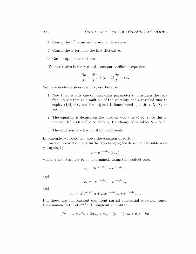
228 CHAPTER 7. THE BLACK-SCHOLES MODEL
4. Cancel the S2 terms in the second derivative.
5. Cancel the S terms in the first derivative.
6. Gather up like order terms.
What remains is the rescaled, constant coefficient equation:
∂v
∂τ=∂2v
∂x2+ (k − 1)
∂v
∂x− kv.
We have made considerable progress, because
1. Now there is only one dimensionless parameter k measuring the risk-free interest rate as a multiple of the volatility and a rescaled time toexpiry (1/2)σ2T , not the original 4 dimensioned quantities K, T , σ2
and r.
2. The equation is defined on the interval −∞ < x < ∞, since this x-interval defines 0 < S <∞ through the change of variables S = Kex.
3. The equation now has constant coefficients.
In principle, we could now solve the equation directly.Instead, we will simplify further by changing the dependent variable scale
yet again, by
v = eαx+βτu(x, τ)
where α and β are yet to be determined. Using the product rule:
vτ = βeαx+βτu+ eαx+βτuτ
and
vx = αeαx+βτu+ eαx+βτux
and
vxx = α2eαx+βτu+ 2αeαx+βτux + eαx+βτuxx.
Put these into our constant coefficient partial differential equation, cancelthe common factor of eαx+βτ throughout and obtain:
βu+ uτ = α2u+ 2αux + uxx + (k − 1)(αu+ ux)− ku

7.2. SOLUTION OF THE BLACK-SCHOLES EQUATION 229
Gather like terms:
uτ = uxx + [2α + (k − 1)]ux + [α2 + (k − 1)α− k − β]u.
Choose α = −(k − 1)/2 so that the ux coefficient is 0, and then chooseβ = α2 + (k − 1)α− k = −(k + 1)2/4 so the u coefficient is likewise 0. Withthis choice, the equation is reduced to
uτ = uxx.
We need to transform the initial condition too. This transformation is
u(x, 0) = e−(−(k−1)/2)x−(−(k+1)2/4)·0v(x, 0)
= e((k−1)/2)x max(ex − 1, 0)
= max(e((k+1)/2)x − e((k−1)/2)x, 0
).
For future reference, we notice that this function is strictly positive whenthe argument x is strictly positive, that is u0(x) > 0 when x > 0, otherwise,u0(x) = 0 for x ≤ 0.
We are in the final stage since we are ready to apply the heat-equationsolution representation formula:
u(x, τ) =1
2√πτ
∫ ∞−∞
u0(s)e−(x−s)2/4τ ds.
However, first we want to make a change of variable in the integration, bytaking z = (s− x) /
√2τ , (and thereby dz = (−1/
√2τ) dx) so that the inte-
gration becomes:
u(x, τ) =1√2π
∫ ∞−∞
u0
(z√
2τ + x)e−z
2/2 dz.
We may as well only integrate over the domain where u0 > 0, that is for
z > −x/√
2τ . On that domain, u0 = e((k+1)/2)·(x+z√
2τ)− e((k−1)/2)·(x+z√
2τ) sowe are down to:
1√2π
∫ ∞−x/√
2τ
ek+12 (x+z
√2τ)e−z
2/2 dz − 1√2π
∫ ∞−x/√
2τ
ek−12 (x+z
√2τ)e−z
2/2 dz
Call the two integrals I1 and I2 respectively.
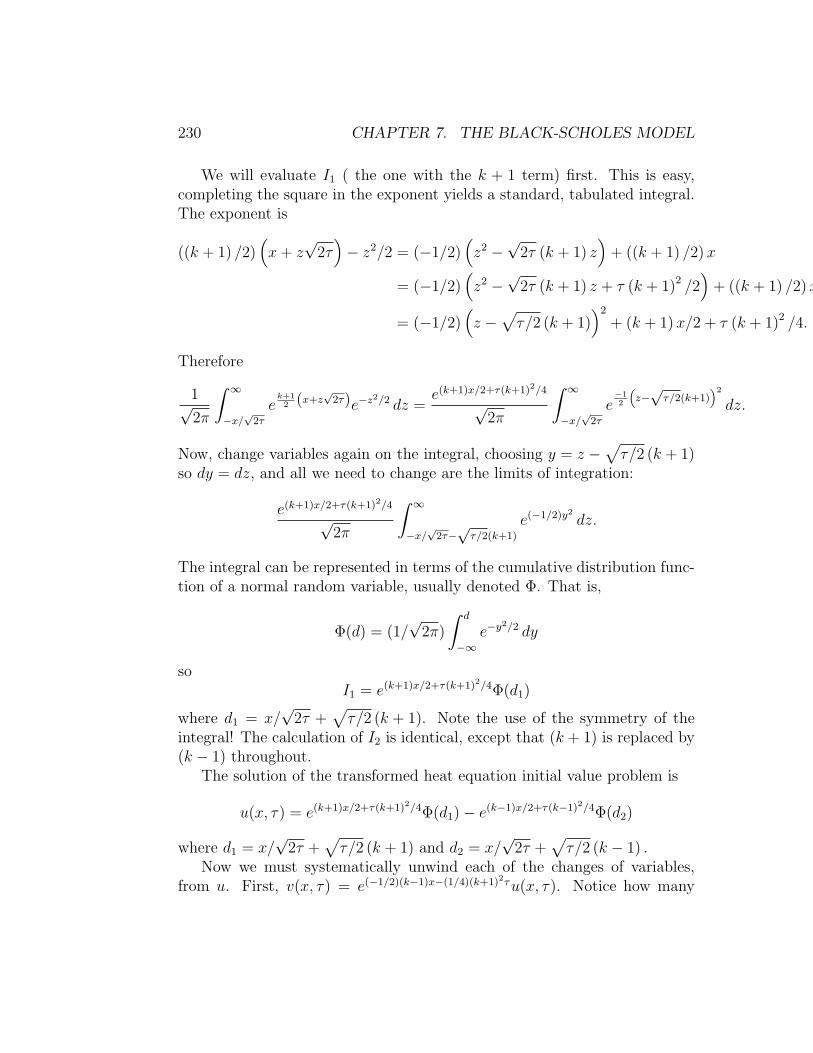
230 CHAPTER 7. THE BLACK-SCHOLES MODEL
We will evaluate I1 ( the one with the k + 1 term) first. This is easy,completing the square in the exponent yields a standard, tabulated integral.The exponent is
((k + 1) /2)(x+ z
√2τ)− z2/2 = (−1/2)
(z2 −
√2τ (k + 1) z
)+ ((k + 1) /2)x
= (−1/2)(z2 −
√2τ (k + 1) z + τ (k + 1)2 /2
)+ ((k + 1) /2)x+ τ (k + 1)2 /4
= (−1/2)(z −
√τ/2 (k + 1)
)2
+ (k + 1)x/2 + τ (k + 1)2 /4.
Therefore
1√2π
∫ ∞−x/√
2τ
ek+12 (x+z
√2τ)e−z
2/2 dz =e(k+1)x/2+τ(k+1)2/4
√2π
∫ ∞−x/√
2τ
e−12
“z−√τ/2(k+1)
”2
dz.
Now, change variables again on the integral, choosing y = z −√τ/2 (k + 1)
so dy = dz, and all we need to change are the limits of integration:
e(k+1)x/2+τ(k+1)2/4
√2π
∫ ∞−x/√
2τ−√τ/2(k+1)
e(−1/2)y2 dz.
The integral can be represented in terms of the cumulative distribution func-tion of a normal random variable, usually denoted Φ. That is,
Φ(d) = (1/√
2π)
∫ d
−∞e−y
2/2 dy
soI1 = e(k+1)x/2+τ(k+1)2/4Φ(d1)
where d1 = x/√
2τ +√τ/2 (k + 1). Note the use of the symmetry of the
integral! The calculation of I2 is identical, except that (k + 1) is replaced by(k − 1) throughout.
The solution of the transformed heat equation initial value problem is
u(x, τ) = e(k+1)x/2+τ(k+1)2/4Φ(d1)− e(k−1)x/2+τ(k−1)2/4Φ(d2)
where d1 = x/√
2τ +√τ/2 (k + 1) and d2 = x/
√2τ +
√τ/2 (k − 1) .
Now we must systematically unwind each of the changes of variables,from u. First, v(x, τ) = e(−1/2)(k−1)x−(1/4)(k+1)2τu(x, τ). Notice how many
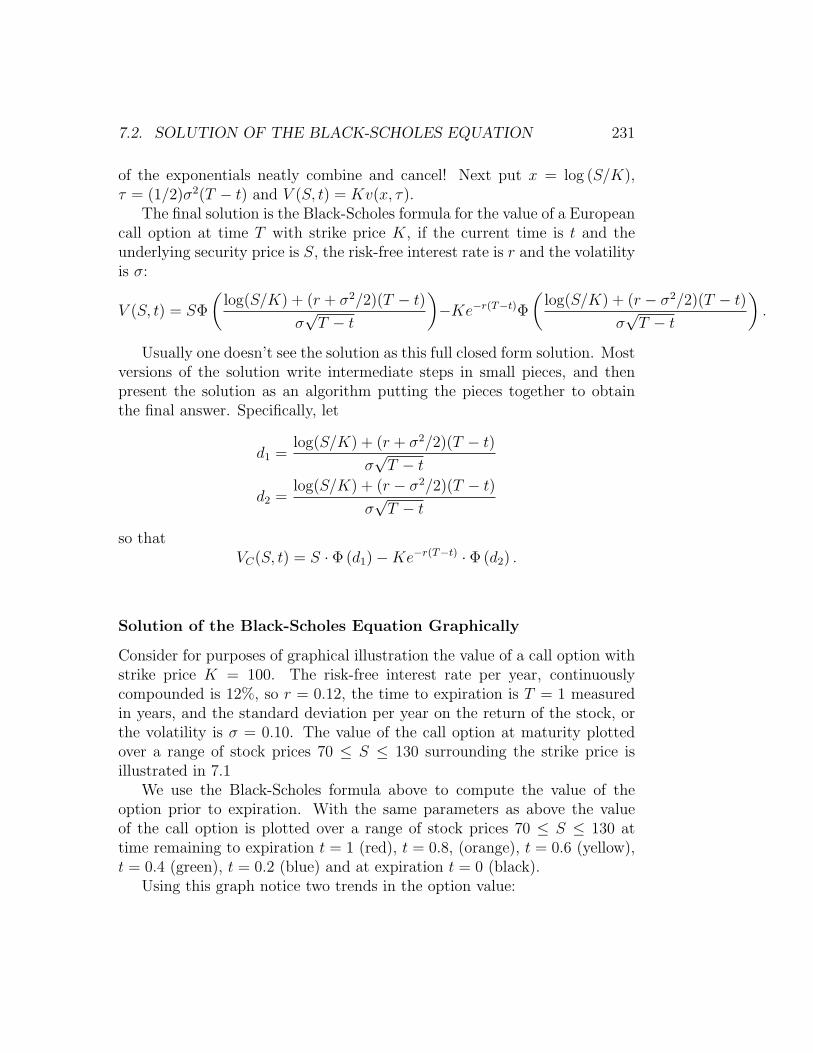
7.2. SOLUTION OF THE BLACK-SCHOLES EQUATION 231
of the exponentials neatly combine and cancel! Next put x = log (S/K),τ = (1/2)σ2(T − t) and V (S, t) = Kv(x, τ).
The final solution is the Black-Scholes formula for the value of a Europeancall option at time T with strike price K, if the current time is t and theunderlying security price is S, the risk-free interest rate is r and the volatilityis σ:
V (S, t) = SΦ
(log(S/K) + (r + σ2/2)(T − t)
σ√T − t
)−Ke−r(T−t)Φ
(log(S/K) + (r − σ2/2)(T − t)
σ√T − t
).
Usually one doesn’t see the solution as this full closed form solution. Mostversions of the solution write intermediate steps in small pieces, and thenpresent the solution as an algorithm putting the pieces together to obtainthe final answer. Specifically, let
d1 =log(S/K) + (r + σ2/2)(T − t)
σ√T − t
d2 =log(S/K) + (r − σ2/2)(T − t)
σ√T − t
so thatVC(S, t) = S · Φ (d1)−Ke−r(T−t) · Φ (d2) .
Solution of the Black-Scholes Equation Graphically
Consider for purposes of graphical illustration the value of a call option withstrike price K = 100. The risk-free interest rate per year, continuouslycompounded is 12%, so r = 0.12, the time to expiration is T = 1 measuredin years, and the standard deviation per year on the return of the stock, orthe volatility is σ = 0.10. The value of the call option at maturity plottedover a range of stock prices 70 ≤ S ≤ 130 surrounding the strike price isillustrated in 7.1
We use the Black-Scholes formula above to compute the value of theoption prior to expiration. With the same parameters as above the valueof the call option is plotted over a range of stock prices 70 ≤ S ≤ 130 attime remaining to expiration t = 1 (red), t = 0.8, (orange), t = 0.6 (yellow),t = 0.4 (green), t = 0.2 (blue) and at expiration t = 0 (black).
Using this graph notice two trends in the option value:
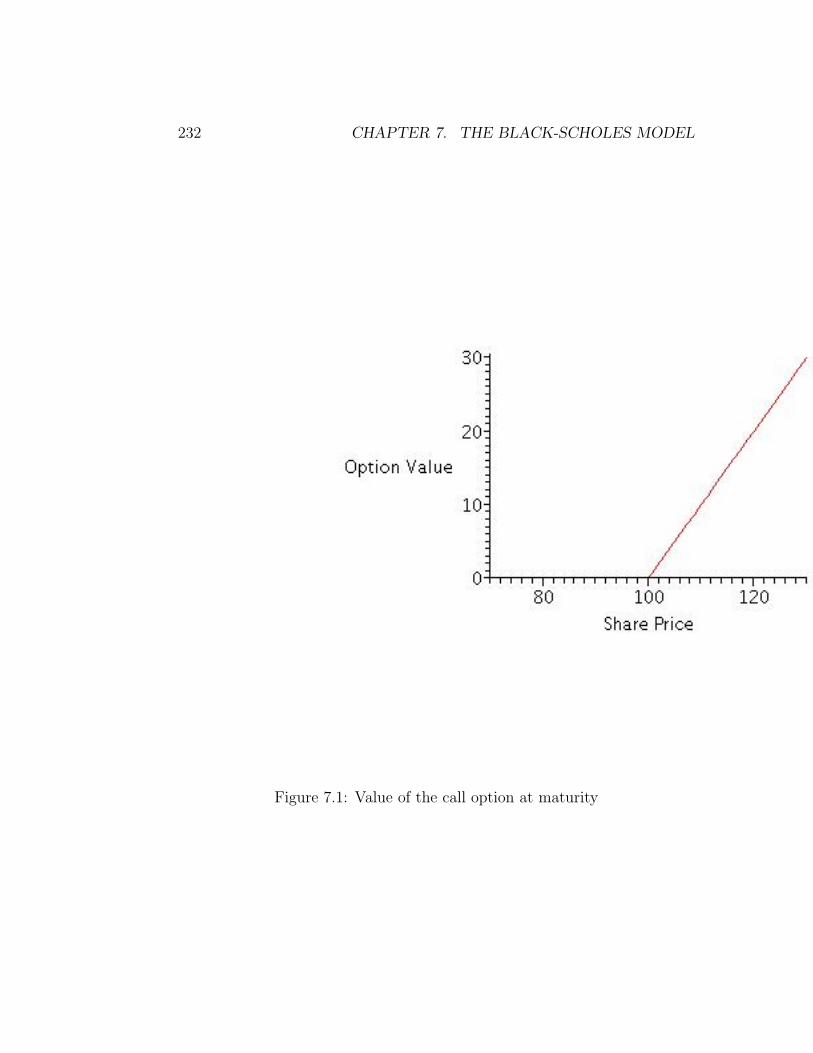
232 CHAPTER 7. THE BLACK-SCHOLES MODEL
Figure 7.1: Value of the call option at maturity

7.2. SOLUTION OF THE BLACK-SCHOLES EQUATION 233
Figure 7.2: Value of the call option at various times
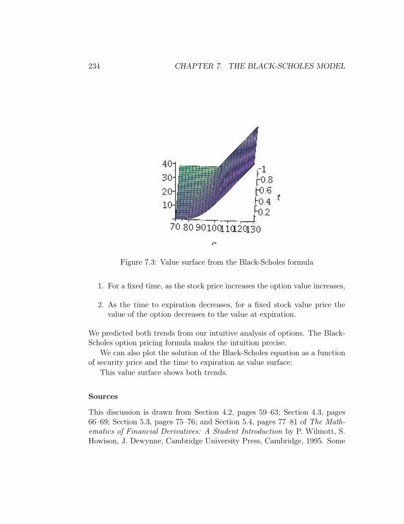
234 CHAPTER 7. THE BLACK-SCHOLES MODEL
Figure 7.3: Value surface from the Black-Scholes formula
1. For a fixed time, as the stock price increases the option value increases,
2. As the time to expiration decreases, for a fixed stock value price thevalue of the option decreases to the value at expiration.
We predicted both trends from our intuitive analysis of options. The Black-Scholes option pricing formula makes the intuition precise.
We can also plot the solution of the Black-Scholes equation as a functionof security price and the time to expiration as value surface:
This value surface shows both trends.
Sources
This discussion is drawn from Section 4.2, pages 59–63; Section 4.3, pages66–69; Section 5.3, pages 75–76; and Section 5.4, pages 77–81 of The Math-ematics of Financial Derivatives: A Student Introduction by P. Wilmott, S.Howison, J. Dewynne, Cambridge University Press, Cambridge, 1995. Some
7.2. SOLUTION OF THE BLACK-SCHOLES EQUATION 235
ideas are also taken from Chapter 11 of Stochastic Calculus and FinancialApplications by J. Michael Steele, Springer, New York, 2001.
Problems to Work for Understanding
1. Explicitly evaluate the integral I2 in terms of the c.d.f. Φ and otherelementary functions as was done for the integral I1.
2. What is the price of a European call option on a non-dividend-payingstock when the stock price is $52, the strike price is $50, the risk-free interest rate is 12% per annum (compounded continuously), thevolatility is 30% per annum, and the time to maturity is 3 months?
3. What is the price of a European call option on a non-dividend payingstock when the stock price is $30, the exercise price is $29, the risk-freeinterest rate is 5%, the volatility is 25% per annum, and the time tomaturity is 4 months?
4. Show that the Black-Scholes formula for the price of a call option tendsto max(S −K, 0) as t→ T .
Outside Readings and Links:
1. Cornell University, Department of Computer Science, Prof. T. Cole-man Rhodes and Prof. R. Jarrow Numerical Solution of Black-ScholesEquation, Submitted by Chun Fan, Nov. 12, 2002.
2. Monash University, Department of Mathematical Science, Eric. W.Chu This link gives some examples and maple commands, Submittedby Chun Fan, Nov. 12, 2002.
3. An applet for calculating the option value based on the Black-Scholesmodel. Also contains tips on options, business news and literature onoptions. Submitted by Yogesh Makkar, November 19, 2003.
4. ExcelEverywhere, a commercial application for spreadsheets on theWeb. A sample spreadsheet based calculator for calculating the optionvalues, based on Black-Scholes model. Submitted by Yogesh Makkar,November 19,2003
236 CHAPTER 7. THE BLACK-SCHOLES MODEL
7.3 Put-Call Parity
Rating
Mathematically Mature: may contain mathematics beyond calculus withproofs.
Section Starter Question
What does it mean to say that a differential equation is a linear differentialequation?
Key Concepts
1. The put-call parity principle links the price of a put option, a call optionand the underlying security price.
2. The put-call parity principle can be used to price European put optionswithout having to solve the Black-Scholes equation.
3. The put-call parity principle is a consequence of the linearity of theBlack-Scholes equation.
Vocabulary
1. The put-call parity principle is the relationship
C − P = S −Ke−r(T−t)
between the price C of a European call option and the price P of aEuropean put option, each with strike price K and underlying securityvalue S.
Mathematical Ideas
Put-Call Parity by Linearity of the Black-Scholes Equation
The Black-Scholes equation is
Vt +1
2σ2S2VSS + rSVS − rV = 0.

7.3. PUT-CALL PARITY 237
With the additional terminal condition V (S, T ) given, a solution exists andis unique. We observe that the Black-Scholes is a linear equation, so thelinear combination of any two solutions is again a solution.
From the problems in the previous section (or by easy verification rightnow) we know that S is a solution of the Black-Scholes equation andKe−r(T−t)
is also a solution, so S −Ke−r(T−t) is a solution. At the expiration time T ,the solution has value S −K.
Now if C(S, t) is the value of a call option at security value S and timet < T , then C(S, t) satisfies the Black-Scholes equation, and has terminalvalue max(S −K, 0). If P (S, t) is the value of a put option at security valueS and time t < T , then P (S, t) also satisfies the Black-Scholes equation, andhas terminal value max(K−S, 0). Therefore by linearity, C(S, t)−P (S, t) isa solution and has terminal value C(S, T )−P (S, T ) = S−K. By uniqueness,the solutions must be the same, and so
C − P = S −Ke−r(T−t).
This relationship is known as the put-call parity principleThis same principle of linearity and the composition of more exotic op-
tions in terms of puts and calls allows us to write closed form formulas forthe values of exotic options such as straps, strangles, and butterfly options.
Put-Call Parity by Reasoning about Arbitrage
Assume that an underlying security satisfies the assumptions of the previoussections. Assume further that:
• The security price is currently S = 100,
• The strike price is K = 100,
• The expiration time is one year, T = 1,
• The risk-free interest rate is r = 0.12,
• The volatility is σ = 0.10.
One can then calculate that the price of a call option with these assumptionsis 11.84.
Consider an investor who buys the following portfolio:

238 CHAPTER 7. THE BLACK-SCHOLES MODEL
• Buy one share of stock at price S = 100.
• Sell one call option at C = V (100, 0) = 11.84.
• Buy one put option at unknown price.
Now at expiration, the stock price could have many different values, andthose would determine the values of the derivatives, see the table for somerepresentative values:
Security Call Put Portfolio80 0 20 10090 0 10 100100 0 0 100110 -10 0 100120 -20 0 100
This portfolio has total value which is the strike price (which happens tobe the same as the current value of the security.) Holding this portfolio willgive a risk-free investment that will pay $100 in any circumstance. Thereforethe value of the whole portfolio must equal the present value of a risklessinvestment that will pay off $100 in one year. This is an illustration of the useof options for hedging an investment, in this case the extremely conservativepurpose of hedging to preserve value.
The parameter values chosen above are not special and we can reasonwith general S, C and P with parameters K, r, σ, and T . Consider buyinga put and selling a call, each with the same strike price K. We will find atexpiration T that
• if the stock price S is below K we will realize a profit of K − S fromthe put option that we own;
• if the stock price is above K, we will realize a loss of S − K fromfulfilling the call option that we sold.
But this payout is exactly what we would get from a futures contract to sellthe stock at price K. The price set by arbitrage of such a futures contractmust be Ke−r(T−t) − S. Specifically, one could sell (short) the stock rightnow for S, and lend Ke−r(T−t) dollars right now for a net cash outlay ofKe−r(T−t) − S, then at time T collect the loan at K dollars and actuallydeliver the stock. This replicates the futures contract, so the future must

7.3. PUT-CALL PARITY 239
have the same price as the initial outlay. Therefore we obtain the put-callparity principle:
−C + P = K exp(−r(T − t))− Sor more naturally
S − C + P = K exp(−r(T − t)).
Synthetic Portfolios
Another way to view this formula is that it instructs us how to create syn-thetic portfolios: Since
S + P −K exp(−r(T − t)) = C
a portfolio “long in the underlying security, long in a put, shortK exp(−r(T−t)) in bonds” replicates a call.
This same principle of linearity and the composition of more exotic op-tions in terms of puts and calls allows us to create synthetic portfolios forthe exotic options such as straddles, strangles, and so on. As noted above,we can easily write their values in closed form solutions.
Explicit Formulas for the Put Option
Knowing any two of S, C or P allows us to calculate the third. Of course,the immediate use of this formula will be to combine the security price andthe value of the call option from the solution of the Black-Scholes equationto obtain the value of the put option:
P = C − S +K exp(−r(T − t))
For the sake of mathematical completeness write the value of a Europeanput option explicitly as:
VP (S, t) = SΦ
(log(S/K) + (r + σ2/2)(T − t)
σ√T − t
)−Ke−r(T−t)Φ
(log(S/K) + (r − σ2/2)(T − t)
σ√T − t
)−S+K exp(−r(T−t)).
Usually one doesn’t see the solution as this full closed form solution.Instead, most versions of the solution write intermediate steps in small pieces,

240 CHAPTER 7. THE BLACK-SCHOLES MODEL
and then present the solution as an algorithm putting the pieces together toobtain the final answer. Specifically, let
d1 =log(S/K) + (r + σ2/2)(T − t)
σ√T − t
d2 =log(S/K) + (r − σ2/2)(T − t)
σ√T − t
so that
VP (S, t) = S(Φ (d1)− 1)−Ke−r(T−t)(Φ (d2)− 1).
Using the symmetry properties of the c.d.f. Φ, we obtain
VP (S, t) = Ke−r(T−t)Φ (−d2)− SΦ (−d1) .
Graphical Views of the Put Option Value
For graphical illustration let P be the value of a put option with strike priceK = 100. The risk-free interest rate per year, continuously compounded is12%, so r = 0.12, the time to expiration is T = 1 measured in years, andthe standard deviation per year on the return of the stock, or the volatilityis σ = 0.10. The value of the put option at maturity plotted over a range ofstock prices 0 ≤ S ≤ 150 surrounding the strike price is illustrated below:
Now we use the Black-Scholes formula to compute the value of the optionprior to expiration. With the same parameters as above the value of the putoption is plotted over a range of stock prices 0 ≤ S ≤ 150 at time remainingto expiration t = 1 (red), t = 0.8, (orange), t = 0.6 (yellow), t = 0.4 (green),t = 0.2 (blue) and at expiration t = 0 (black).
Notice a couple of trends in the value from this graph:
1. As the stock price increases, for a fixed time the option value decreases,
2. As the time to expiration decreases, for a fixed stock value price lassthan the strike price the value of the option increases to the value atexpiration.
We can also plot the value of the put option as a function of security priceand the time to expiration as value surface:
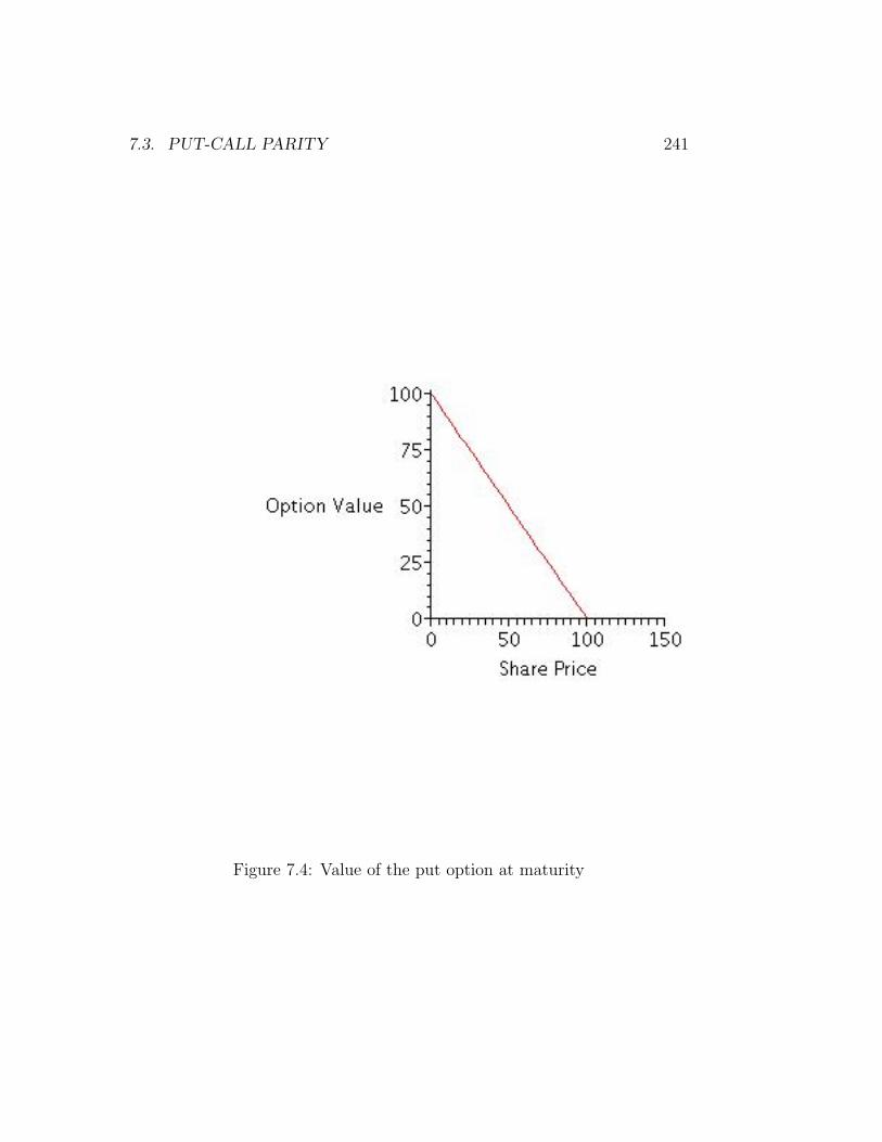
7.3. PUT-CALL PARITY 241
Figure 7.4: Value of the put option at maturity
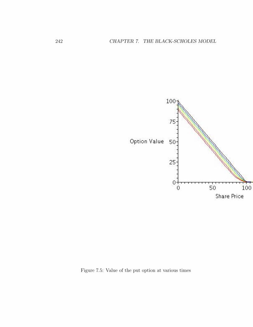
242 CHAPTER 7. THE BLACK-SCHOLES MODEL
Figure 7.5: Value of the put option at various times

7.3. PUT-CALL PARITY 243
Figure 7.6: Value surface from the put-call parity formula

244 CHAPTER 7. THE BLACK-SCHOLES MODEL
Sources
This section is adapted from: Financial Derivatives by Robert W. Kolb,New York Institute of Finance, Englewood Cliffs, NJ, 1993, page 107 andfollowing. Parts are also adapted from Stochastic Calculus and FinancialApplications by J. Michael Steele, Springer, New York, 2000, page 155.
Problems to Work for Understanding
1. Calculate the price of a 3-month European put option on a non-dividend-paying stock with a strike price of $50 when the current stock price is$50, the risk-free interest rate is 10% per annum (compounded contin-uously) and the volatility is 30% per annum.
2. What is the price of a European put option on a non-dividend payingstock when the stock price is $69, the strike price is $70, the risk-free interest rate is 5% per annum (compounded continuously), thevolatility is 35% per annum, and the time to maturity is 6 months?
Outside Readings and Links:
1. Video with explanation of put-call parity.
2. Option Research and Technology Services Provides important optiontrading terms and jargon, here is the link to definition of “Put-CallParity”.
7.4 Derivation of the Black-Scholes Equation
Rating
Mathematically Mature: may contain mathematics beyond calculus withproofs.
Section Starter Question
What is the most important idea in the derivation of the binomial optionpricing model?
7.4. DERIVATION OF THE BLACK-SCHOLES EQUATION 245
Key Concepts
1. The derivation of the Black-Scholes equation uses
(a) tools from calculus,
(b) the quadratic variation of Geometric Brownian Motion,
(c) the no-arbitrage condition to evaluate growth of non-risky portfo-lios,
(d) and a simple but profound insight to eliminate the randomness orrisk.
Vocabulary
1. A backward parabolic PDE is a partial differential equation of theform Vt + DVxx + . . . = 0 with highest derivative terms in t of order1 and highest derivative terms x of order 2 respectively. Terminalvalues V (S, T ) at an end time t = T must be satisfied in contrast tothe initial values at t = 0 required by many problems in physics andengineering.
2. A terminal condition for a backward parabolic equation is the speci-fication of a function at the end time of the interval of consideration touniquely determine the solution. It is analogous to an initial conditionfor an ordinary differential equation, except that it occurs at the endof the time interval, instead of the beginning.
Mathematical Ideas
Explicit Assumptions Made for Modeling and Derivation
For mathematical modeling of a market for a risky security we will ideallyassume
1. that a large number of identical, rational traders always have completeinformation about all assets they are trading,
2. changes in prices are given by a continuous random variable with someprobability distribution,
3. that trading transactions take negligible time,
246 CHAPTER 7. THE BLACK-SCHOLES MODEL
4. purchases and sales can be made in any amounts, that is, the stock andbond are divisible, we can buy them in any amounts including negativeamounts (which are short positions),
5. the risky security issues no dividends.
The first assumption is the essence of what economists call the efficientmarket hypothesis. The efficient market hypothesis leads to the secondassumption as a conclusion, called the random walk hypothesis. Anotherversion of the random walk hypothesis says that traders cannot predict thedirection of the market or the magnitude of the change in a stock so thebest predictor of the market value of a stock is the current price. We willmake the second assumption stronger and more precise by specifying theprobability distribution of the changes with a stochastic differential equation.The remaining hypotheses are simplifying assumptions which can be relaxedat the expense of more difficult mathematical modeling.
We wish to find the value V of a derivative instrument based on anunderlying security which has value S. Mathematically, we assume
1. the price of the underlying security follows the stochastic differentialequation
dS = rS dt+ σS dW
or equivalently that S(t) is a Geometric Brownian Motion with param-eters r − σ2/2 and σ,
2. the risk free interest rate r and the volatility σ are constants,
3. the value V of the derivative depends only on the current value of theunderlying security S and the time t, so we can write V (S, t),
4. All variables are real-valued, and all functions are sufficiently smoothto justify necessary calculus operations.
The first assumption is a mathematical translation of a strong form ofthe efficient market hypothesis from economics. It is a reasonable modelingassumption but finer analysis strongly suggests that security prices have ahigher probability of large price swings than Geometric Brownian Motionpredicts. Therefore the first assumption is not supported by data. However,it is useful since we have good analytic understanding of Geometric BrownianMotion.
7.4. DERIVATION OF THE BLACK-SCHOLES EQUATION 247
The second assumption is a reasonable assumption for a modeling attemptalthough good evidence indicates neither interest rates nor the volatility areconstant. On reasonably short times scales, say a period of three monthsfor the lifetime of most options, the interest rate and the volatility are ap-proximately constant. The third and fourth assumptions are mathematicaltranslations of the assumptions that securities can be bought and sold inany amount and that trading times are negligible, so that standard tools ofmathematical analysis can be applied. Both assumptions are reasonable formodern security trading.
Derivation of the Black-Scholes equation
We consider a simple derivative instrument, an option written on an under-lying asset, say a stock that trades in the market at price S(t). A payofffunction Λ(S) determines the value of the option at expiration time T . Fort < T , the option value should depend on the underlying price S and thetime t. We denote the price as V (S, t). So far all we know is the value at thefinal time V (S, T ) = Λ(S). We would like to know the value V (S, 0) so thatwe know an appropriate buying or selling price of the option.
As time passes, the value of the option changes, both because the ex-piration date approaches and because the stock price changes. We assumethe option price changes smoothly in both the security price and the time.Across a short time interval δt we can write by the Taylor series expansionof V that:
δV = Vtδt+ VsδS +1
2VSS(δS)2 + . . .
The neglected terms are of order (δt)2, δSδt, and (δS)3 and higher. We relyon our intuition from random walks and Brownian motion to explain why wekeep the terms of order (δS)2 but neglect the other terms. More about thislater.
To determine the price, we construct a replicating portfolio. This willbe a specific investment strategy involving only the stock and a cash accountthat will yield exactly the same eventual payoff as the option in all possiblefuture scenarios. Its present value must therefore be the same as the presentvalue of the option and if we can determine one we can determine the other.We thus define a portfolio Π consisting of φ(t) shares of stock and ψ(t) unitsof the cash account B(t). The portfolio constantly changes in value as thesecurity price changes randomly and the cash account accumulates interest.

248 CHAPTER 7. THE BLACK-SCHOLES MODEL
In a short time interval, we can take the changes in the portfolio to be
δΠ = φ(t)δS + ψ(t)rB(t)δt
since δB(t) ≈ rB(t)δt, where r is the interest rate. This says that short-time changes in the portfolio value are due only to changes in the securityprice, and the interest growth of the cash account, and not to additions orsubtraction of the portfolio amounts. Any additions or subtractions are dueto subsequent reallocations financed through the changes in the componentsthemselves.
The difference in value between the two portfolios changes by
δ(V − Π) = (Vt − ψ(t)rB(t))δt+ (VS − φ(t))δS +1
2VSS(δS)2 + . . . .
This could be considered to be a three-part portfolio consisting of an option,and short-selling φ units of the security and ψ units of bonds.
Next come a couple of linked insights: As an initial insight we will elim-inate the first order dependence on S by taking φ(t) = VS. Note that thismeans the rate of change of the derivative value with respect to the securityvalue determines a policy for φ(t). Looking carefully, we see that this pol-icy removes the “randomness” from the equation for the difference in values!(What looks like a little “trick” right here hides a world of probability theory.This is really a Radon-Nikodym derivative that defines a change of measurethat transforms a diffusion, i.e. a transformed Brownian motion with drift,to a standard Wiener measure.)
Second, since the difference portfolio is now non-risky, it must grow invalue at exactly the same rate as any risk-free bank account:
δ(V − Π) = r(V − Π)δt.
This insight is actually our now familiar no-arbitrage-possibility argument: Ifδ(V −Π) > r(V −Π)δt, then anyone could borrow money at rate r to acquirethe portfolio V − Π, holding the portfolio for a time δt, and then sellingthe portfolio, with the growth in the difference portfolio more than enoughto cover the interest costs on the loan. On the other hand if δ(V − Π) <r(V −Π)δt, then short-sell the option in the marketplace for V , purchase φ(t)shares of stock and loan the rest of the money out at rate r. The interestgrowth of the money will more than cover the repayment of the difference

7.4. DERIVATION OF THE BLACK-SCHOLES EQUATION 249
portfolio. Either way, the existence of risk-free profits to be made in themarket will drive the inequality to an equality.
So:
r(V − Π)δt = (Vt − ψ(t)rB(t))δt+1
2VSS(δS)2.
Recall the quadratic variation of Geometric Brownian Motion is determinis-tic, namely (δS)2 = σ2S(t)2δt,
r(V − Π)δt = (Vt − ψ(t)rB(t))δt+1
2σ2S2VSSδt.
Cancel the δt terms, and recall that V − Π = V − φ(t)S − ψ(t)B(t), andφ(t) = VS, so that on the left r(V −Π) = rV − rVSS− rψ(t)B(t). The terms−rψ(t)B(t) on left and right cancel, and we are left with the Black-Scholesequation:
Vt +1
2σ2S2VSS + rSVS − rV = 0.
Note that under the assumptions made for the purposes of the modelingthe partial differential equation depends only on the constant volatility σand the constant risk-free interest rate r. This partial differential equation(PDE) must be satisfied by the value of any derivative security dependingon the asset S.
Some comments about the PDE:
• The PDE is linear: Since the solution of the PDE is the worth of theoption, then two options are worth twice as much as one option, and aportfolio consisting two different options has value equal to the sum ofthe individual options.
• The PDE is backwards parabolic because of the form Vt+(1/2)σ2S2VSS.Thus, terminal values V (S, T ) (in contrast to the initial values re-quired by many problems in physics and engineering) must be specified.The value of a European option at expiration is known as a function ofthe security price S, so we have a terminal value. The PDE is solved todetermine the value of the option at times before the expiration date.
Comment on the derivation:
The derivation above follows reasonably closely the original derivation ofBlack, Scholes and Merton. Option prices can also be calculated and the

250 CHAPTER 7. THE BLACK-SCHOLES MODEL
Black-Scholes equation derived by more advanced probabilistic methods. Inthis equivalent formulation, the discounted price process exp(−rt)S(t) isshifted into a “risk-free” measure using the Cameron-Martin-Girsanov The-orem, so that it becomes a martingale. The option price V (S, t) is then thediscounted expected value of the payoff Λ(t) in this measure, and the PDEis obtained as the backward evolution equation for the expectation. Thederivation above follows the classical derivation of Black and Scholes, butthe probabilistic view is more modern and can be more easily extended togeneral market models.
The derivation of the Black-Scholes equation above uses the fairly intu-itive partial derivative equation approach because of the simplicity of thederivation. This derivation:
• is easily motivated and related to similar derivations of partial differ-ential equations in physics and engineering,
• avoids the burden of developing additional probability theory and mea-sure theory machinery, including filtrations, sigma-fields, previsibility,and changes of measure including Radon-Nikodym derivatives and theCameron-Martin-Girsanov theorem.
• also avoids, or at least hides, martingale theory that we have not yetdeveloped or exploited,
• does depend on the stochastic process knowledge that we have gainedalready, but not more than that knowledge!
The disadvantages are that:
• we are forced to skim certain details relying on motivation instead ofstrict mathematical rigor,
• when we are done we still have to solve the partial differential equationto get the price on the derivative, whereas the probabilistic methods de-liver the solution almost automatically and give the partial differentialequation as an auxiliary by-product,
• the probabilistic view is more modern and can be more easily extendedto general market models.
7.4. DERIVATION OF THE BLACK-SCHOLES EQUATION 251
Sources
This derivation of the Black-Scholes equation is drawn from “Financial Deriva-tives and Partial Differential Equations” by Robert Almgren, in AmericanMathematical Monthly, Volume 109, January, 2002, pages 1–11.
Problems to Work for Understanding
1. Show by substitution that two exact solutions of the Black-Scholesequations are
(a) V (S, t) = AS, A some constant.
(b) V (S, t) = Aexp(rt)
Explain in financial terms what each of these solutions represents. Thatis, describe a simple “claim”, “derivative” or “option” for which thissolution to the Black Scholes equation gives the value of the claim atany time.
2. Draw the expiry diagrams (that is, a graph of terminal condition ofportfolio value versus security price S) at the expiration time for theportfolio which is
(a) Short one share, long two calls with exercise price K. (This iscalled a straddle .)
(b) Long one call, and one put both exercise price K. (This is alsocalled a straddle.)
(c) Long one call, and two puts, all with exercise price K. (This iscalled a strip .)
(d) Long one put, and two calls, all with exercise price K. (This iscalled a strap .)
(e) Long one call with exercise price K1 and one put with exerciseprice K2. Compare the three cases when K1 > K2, (known as astrangle), K1 = K2, and K1 < K2.
(f) As before, but also short one call and one put with exercise priceK. (When K1 < K < K2, this is called a butterfly spread. )

252 CHAPTER 7. THE BLACK-SCHOLES MODEL
Outside Readings and Links:
1. Bradley University, School of Business Administration, Finance De-partment, Kevin Rubash A very brief description on the developmenthistory of option theory and the Black-Scholes model for calculatingoption value, with the notations, Greeks and some explanatory graphs.Also contains a calculators for the option value calculation. Submittedby Yogesh Makkar, November 19, 2003.
7.5 Implied Volatility
Rating
Mathematically Mature: may contain mathematics beyond calculus withproofs.
Section Starter Question
What are some methods you could use to find the solution of f(x) = c for xwhere f is a function that is so complicated that you cannot use elementaryfunctions and operations to isolate x ?
Key Concepts
1. We estimate historical volatility by applying the standard deviationestimator from statistics to the observations ln(Si/Si−1).
2. We deduce implied volatility by numerically solving the Black-Scholesformula for σ.
Vocabulary
1. Historical volatility of a security is the variance of the changes inthe logarithm of the price of the underlying asset, obtained from pastdata.
2. Implied volatility of a security is the numerical value of the volatilityparameter that makes the market price of an option equal to the valuefrom the Black-Scholes formula.

7.5. IMPLIED VOLATILITY 253
Mathematical Ideas
Historical volatility
Estimates of historical volatility of security prices use statistical estima-tors, usually one of the estimators of variance. A main problem for historicalvolatility is to select the sample size, or window of observations, used to es-timate σ2. Different time-windows usually give different volatility estimates.Furthermore, for a lot of customized “over the counter” derivatives, the nec-essary price data may not exist.
Another problem with historical volatility is that it assumes future marketperformance is the same as past market data. Although this is a naturalscientific assumption, it does not take into account historical anomalies suchas the October 1987 stock market drop, which may be unusual. That is,computing historical volatility has the usual statistical difficulty of how tohandle outliers. The assumption that future market performance is the sameas past performance also does not take into account underlying changes inthe market such as economic conditions.
To estimate the volatility of a security price empirically, observe the secu-rity price at regular intervals, such as every day, every week, or every month.Define:
1. the number of observations n+ 1
2. Si, i = 0, 1, 2, 3, . . . , n is the security price at the end of the ith interval,
3. τ is the length of each of the time intervals (say in years),
and let
ui = ln(Si)− ln(Si−1) = ln
(SiSi−1
)for i = 1, 2, 3, . . . be the increment of the logarithms of the security prices.We are modeling the security price as a Geometric Brownian Motion, so thatln(Si)− ln(Si−1) ∼ N(rτ, σ2τ).
Since Si = Si−1eui , ui is the continuously compounded return, (not an-
nualized) in the ith interval. Then the usual estimate s, of the standarddeviation of the ui’s is
s =
√√√√ 1
n− 1
n∑i=1
(ui − u)2

254 CHAPTER 7. THE BLACK-SCHOLES MODEL
where u is the mean of the ui’s. Sometimes it is more convenient to use theequivalent formula
s =
√√√√ 1
n− 1
n∑i=1
u2i −
1
n(n− 1)
(n∑i=1
ui
)2
.
We assume the security price varies as a Geometric Brownian Motion.That means that the logarithm of the security price is a Wiener process withsome drift and on the period of time τ , would have a variance σ2τ . Therefore,s is an estimate of σ
√t. It follows that σ can be estimated as
σ ≈ s√τ.
Choosing an appropriate value for n is not obvious. Remember the vari-ance expression for Geometric Brownian Motion is an increasing function oftime. If we model security prices with Geometric Brownian Motion, thenσ does change over time, and data that are too old may not be relevantfor the present or the future. A compromise that seems to work reasonablywell is to use closing prices from daily data over the most recent 90 to 180days. Empirical research indicates that only trading days should be used, sodays when the exchange is closed should be ignored for the purposes of thevolatility calculation. [22, page 215]
Economists and financial analysts often estimate historical volatility withmore sophisticated statistical time series methods.
Implied Volatility
The implied volatility is the parameter σ in the Black-Scholes formulathat would give the option price that is observed in the market, all otherparameters being known.
The Black-Scholes formula is complicated to “invert” to explicitly ex-press σ as a function of the other parameters. Therefore, we use numericaltechniques to implicitly solve for σ. A simple idea is to use the method ofbisection search to find σ.
Example. Suppose the value of a call on a non-dividend paying security is1.85 when S = 21, K = 20, r = 0.10, and T − t = 0.25 and σ is unknown.We start by arbitrarily guessing σ = 0.20. The Black-Scholes formula gives
7.5. IMPLIED VOLATILITY 255
C = 1.7647, which is too low. Since C is a increasing function of σ, thissuggests we try a value of σ = 0.30. This gives C = 2.1010, too high, sowe bisect the interval [0.20, 0.30] and try σ = 0.25. This value of σ givesa value of C = 1.9268, still too high. Bisect the interval [0.20, 0.25] andtry a value of σ = 0.225, which yields C = 1.8438, slightly too low. Tryσ = 0.2375, giving C = 1.8849. Finally try σ = 0.23125 giving C = 1.8642.To 2 significant digits, the significance of the data, σ = 0.23, with a predictedvalue of C = 1.86.
A faster procedure is to use Newton’s method which is iterative. Essen-tially we are trying to solve
f(σ, S,K, r, T − t)− C = 0,
so from an initial guess σ0, we form the Newton iterates
σi+1 = σi − f(σi)/(df(σi)/dσ).
This means one has to differentiate the Black-Scholes formula with respectto σ. This derivative is one of the “Greeks” known as vega which we will lookat more extensively in the next section. A formula for vega for a Europeancall option is
df
dσ= S√T − tΦ′(d1) exp(−r(T − t)).
A natural way to do the iteration is with a computer program rather thanby hand.
Implied volatility is a “forward-looking” estimation technique, in contrastto the “backward-looking” historical volatility. That is, it incorporates themarket’s expectations about the prices of securities and their derivatives, ormore concisely, market expectations about risk. More sophisticated com-binations and weighted averages combining estimates from several differentderivative claims can be developed.
Sources
This section is adapted from: Quantitative modeling of Derivative Securitiesby Marco Avellaneda, and Peter Laurence, Chapman and Hall, Boca Raton,2000, page 66; and Options, Futures, and other Derivative Securities secondedition, by John C. Hull, Prentice Hall, 1993, pages 229–230.

256 CHAPTER 7. THE BLACK-SCHOLES MODEL
Problems to Work for Understanding
1. Suppose that the observations on a security price (in dollars) at the endof each of 15 consecutive weeks are as follows: 30.25, 32, 31.125, 30.25,30.375, 30.625, 33, 32.875, 33, 33.5, 33.5 33.75, 33.5, 33.25. Estimatethe security price volatility.
2. A call option on a non-dividend paying security has a market price of$2.50. The security price is $15, the exercise price is $13, the time tomaturity is 3 months, and the risk-free interest rate is 5% per year.What is the implied volatility?
Outside Readings and Links:
1. Peter Hoadley, Options Strategy Analysis Tools has a Historic VolatilityCalculator that calculates and graphs historic volatility using historicalprice data retrieved from Yahoo.com. Submitted by Bashar Al-Salim,Dec. 2, 2003.
2. Analysis of asset allocation A calculator to compute implied volatilityusing Black and Scholes. Submitted by Bashar Al-Salim, Dec. 2, 2003.
3. MindXpansion,a Tool for Option Traders This option calculator pack-ages an enormous amount of functionality onto one screen, calculatingimplied volatility or historical volatility with Midas Touch. Submittedby Chun Fan, Dec. 3, 2003.
7.6 Sensitivity, Hedging and the “Greeks”
Rating
Mathematically Mature: may contain mathematics beyond calculus withproofs.
Section Starter Question
Key Concepts
1. The sensitivity of the Black-Scholes formula to each of the variablesand parameters is named, is fairly easily expressed, and has important
7.6. SENSITIVITY, HEDGING AND THE “GREEKS” 257
consequences for hedging investments.
2. The sensitivity of the Black-Scholes formula (or any mathematicalmodel) to its parameters is important for understanding the modeland its utility.
Vocabulary
1. The Delta (∆) of a financial derivative is the rate of change of thevalue with respect to the value of the underlying security, in symbols
∆ =∂V
∂S
2. The Gamma (Γ) of a derivative is the sensitivity of ∆ with respect toS, in symbols
Γ =∂2V
∂S2.
3. The Theta (Θ) of a European claim with value function V (S, t) isdefined as
Θ =∂V
∂t.
4. The rho (ρ) of a derivative security is the rate of change of the valueof the derivative security with respect to the interest rate, in symbols
ρ =∂V
∂r.
5. The Vega (Λ) of derivative security is the rate of change of value ofthe derivative with respect to the volatility of the underlying asset, insymbols
Λ =∂V
∂σ.
6. Hedging is the attempt to make a portfolio value immune to smallchanges in the underlying asset value (or its parameters).

258 CHAPTER 7. THE BLACK-SCHOLES MODEL
Figure 7.7: Value of the call option at various times
Mathematical Ideas
To start the examination of each of the sensitivities, restate the Black-Scholesformula for the value of a European call option:
d1 =log(S/K) + (r + σ2/2)(T − t)
σ√T − t
d2 =log(S/K) + (r − σ2/2)(T − t)
σ√T − t
and then
VC(S, t) = SΦ (d1)−Ke−r(T−t)Φ (d2) .
Note that d2 = d1 − σ2√T − t.
7.6. SENSITIVITY, HEDGING AND THE “GREEKS” 259
Delta
The Delta of a European call option is the rate of change of its value withrespect to the underlying security price:
∆ =∂VC∂S
= Φ(d1) + SΦ′(d1)∂d1
∂S
−K exp(−r(T − t))Φ′(d2)∂d2
∂S
= Φ(d1) + S1√2π
exp(−d21/2)
1
Sσ√T − t
−K exp(−r(T − t)) 1√2π
exp(−d22/2)
1
Sσ√T − t
= Φ(d1) + S1√2π
exp(−d21/2)
1
Sσ√T − t
−K exp(−r(T − t)) 1√2π
exp
(−(d1 − σ
√T − t
)2
/2
)1
Sσ√T − t
= Φ(d1) +exp(−d2
1/2)√2πσ√T − t
×[1− K exp(−r(T − t))
Sexp
(d1σ√T − t− σ2(T − t)/2
)]= Φ(d1) +
exp(−d21/2)√
2πσ√T − t
×[1− K exp(−r(T − t))
Sexp
(log(S/K) + (r + σ2/2)(T − t)− σ2(T − t)/2
)]= Φ(d1) +
exp(−d21/2)√
2πσ√T − t
×[1− K exp(−r(T − t))
Sexp (log(S/K) + r(T − t))
]= Φ(d1)
Note that since 0 < Φ(d1) < 1 (for all reasonable values of d1), ∆ > 0, andso the value of a European call option is always increasing as the underlyingsecurity value increases. This is precisely as we intuitively predicted when
260 CHAPTER 7. THE BLACK-SCHOLES MODEL
we first considered options, see Options. The increase in security value in Sis visible in Figure 7.7.
Delta Hedging
Notice that for any sufficiently differentiable function F (S)
F (S1)− F (S2) ≈dF
dS(S1 − S2)
Therefore, for the Black-Scholes formula for a European call option, usingour current notation ∆ = ∂V/∂S,
(V (S1)− V (S2))−∆(S1 − S2) ≈ 0
or equivalently for small changes in security price from S1 to S2,
V (S1)−∆S1 ≈ V (S2)−∆S2.
In financial language, we express this as:
“long 1 derivative, short ∆ units of the underlying asset ismarket neutral for small changes in the asset value.”
We say that the sensitivity ∆ of the financial derivative value with respectto the asset value gives the hedge-ratio. The hedge-ratio is the number ofshort units of the underlying asset which combined with a call option willoffset immediate market risk. After a change in the asset value, ∆(S) willalso change, and so we will need to dynamically adjust the hedge-ratio tokeep pace with the changing asset value. Thus ∆(S) as a function of Sprovides a dynamic strategy for hedging against risk.
We have seen this strategy before. In the derivation of Black-Scholesequation, we required that the amount of security in our portfolio, namelyφ(t) be chosen so that φ(t) = VS. See Derivation of the Black-Scholes Equa-tion The choice φ(t) = VS gave us a risk-free portfolio which must change inthe same way as a risk-free asset.
Gamma: The convexity factor
The Gamma (Γ) of a derivative is the sensitivity of ∆ with respect to S:
Γ =∂2V
∂S2.

7.6. SENSITIVITY, HEDGING AND THE “GREEKS” 261
The concept of Gamma is important when the hedged portfolio cannotbe adjusted continuously in time according to ∆(S(t)). If Gamma is smallthen Delta changes very little with S. This means the portfolio requires onlyinfrequent adjustments in the hedge-ratio. However, if Gamma is large, thenthe hedge-ratio Delta is sensitive to changes in the price of the underlyingsecurity.
According to the Black-Scholes formula, we have
Γ =1
S√
2πσ√T − t
exp(−d21/2)
Notice that Γ > 0, so the call option value is always concave-up with respectto S. See this in Figure 7.7.
Theta: The time decay factor
The Theta (Θ) of a European claim with value function V (S, t) is definedas
Θ =∂V
∂t.
Note that this definition is the rate of change with respect to the real (orcalendar) time, some other authors define the rate of change with respect tothe time-to-expiration T − t, so be careful when reading.
The Theta of a claim is sometimes refereed to as the time decay of theclaim. For a European call option on a non-dividend-paying stock,
Θ = − S · σ2√T − t
· exp(−d21/2)√
2π− rK exp(−r(T − t))Φ(d2).
Note that Θ for a European call option is negative, so the value of a Europeancall option is decreasing as a function of time, confirming what we intuitivelydeduced before. See this in Figure 7.7.
Theta does not act like a hedging parameter as do Delta and Gamma.Although there is uncertainty about the future stock price, there is no un-certainty about the passage of time. It does not make sense to hedge againstthe passage of time on an option.
Note that the Black-Scholes partial differential equation can now be writ-ten as
Θ + rS∆ +1
2σ2S2Γ = rV.

262 CHAPTER 7. THE BLACK-SCHOLES MODEL
Given the parameters r, and σ2, and any 4 of Θ, ∆, Γ, S and V the remainingquantity is implicitly determined.
Rho: The interest rate factor
The rho (ρ) of a derivative security is the rate of change of the value ofthe derivative security with respect to the interest rate. It measures thesensitivity of the value of the derivative security to interest rates. For aEuropean call option on a non-dividend paying stock,
ρ = K(T − t) exp(−r(T − t))Φ(d2)
so ρ is always positive. An increase in the risk-free interest rate means acorresponding increase in the derivative value.
Vega: The volatility factor
The Vega (Λ) of a derivative security is the rate of change of value of thederivative with respect to the volatility of the underlying asset. (Note, someauthors also denote Vega by variously λ, κ and σ and refer to Vega by thecorresponding proper Greek letter name.) For a European call option on anon-dividend-paying stock,
Λ = S√T − texp(−d2
1/2)√2π
so the Vega is always positive. An increase in the volatility will lead toa corresponding increase in the call option value. These formulas implicitlyassume that the price of an option with variable volatility (which we have notderived, we explicitly assumed volatility was a constant!) is the same as theprice of an option with constant volatility. To a reasonable approximationthis seems to be the case, for more details and references, see [22, page 316].
Hedging in Practice
It would be wrong to give the impression that traders continuously balancetheir portfolios to maintain Delta neutrality, Gamma neutrality, Vega neu-trality, and so on as would be suggested by the continuous mathematical

7.6. SENSITIVITY, HEDGING AND THE “GREEKS” 263
formulas presented above. In practice, transaction costs make frequent bal-ancing expensive. Rather than trying to eliminate all risks, an option traderusually concentrates on assessing risks and deciding whether they are accept-able. Traders tend to use Delta, Gamma, and Vega measures to quantify thedifferent aspects of risk in their portfolios.
Sources
The material in this section is adapted from ‘Quantitative modeling of Deriva-tive Securities by Marco Avellaneda, and Peter Laurence, Chapman and Hall,Boca Raton, 2000, pages 44–56,; and Options, Futures, and other DerivativeSecurities second edition, by John C. Hull, Prentice Hall, 1993, pages 298–318.
Problems to Work for Understanding
1. How can a short position in 1,000 call options be made Delta neutralwhen the Delta of each option is 0.7?
2. Calculate the Delta of an at-the-money 6-month European call optionon a non-dividend paying stock, when the risk-free interest rate is 10%per year (compound continuously) and the stock price volatility is 25%per year.
3. Use the put-call parity relationship to derive the relationship between
(a) The Delta of European call and the Delta of European put.
(b) The Gamma of European call and the Gamma of European put.
(c) The Vega of a European call and a European put.
(d) The Theta of European call and a European put.
4. (a) Derive the expression for Γ for a European call option as given inthe notes.
(b) Draw a graph of Γ versus S for K = 50, r = 0.10, σ = 0.25,T − t = 0.25.
(c) Draw a graph of Γ versus t for a call option on an at-the-moneystock, with K = 50, r = 0.10, σ = 0.25, T − t = 0.25.
264 CHAPTER 7. THE BLACK-SCHOLES MODEL
(d) Draw the graph of Γ versus S and t for a European call optionwith K = 50, r = 0.10, σ = 0.25, T − t = 0.25.
(e) Comparing the graph of Γ versus S and t with the graph of VCversus S and t in of Solution the Black Scholes Equation, explainthe shape and values of the Γ graph. This only requires an under-standing of calculus, not financial concepts.
5. (a) Derive the expression for Θ for a European call option, as givenin the notes.
(b) Draw a graph of Θ versus S for K = 50, r = 0.10, σ = 0.25,T − t = 0.25.
(c) Draw a graph of Θ versus t for an at-the-money stock, with K =50, r = 0.10, σ = 0.25, T = 0.25.
6. (a) Derive the expression for ρ for a European call option as given inthis section.
(b) Draw a graph of ρ versus S for K = 50, r = 0.10, σ = 0.25,T − t = 0.25.
7. (a) Derive the expression for Λ for a European call option as given inthis section.
(b) Draw a graph of Λ versus S for K = 50, r = 0.10, σ = 0.25,T − t = 0.25.
Outside Readings and Links:
1. Stock Option Greeks video on the meaning and interpretation of therates of change of stock options with respect to parameters.
7.7 Limitations of the Black-Scholes Model
Rating
Student: contains scenes of mild algebra or calculus that may require guid-ance.

7.7. LIMITATIONS OF THE BLACK-SCHOLES MODEL 265
Section Starter Question
We have derived and solved the Black-Scholes equation. We have derivedparameter dependence and sensitivity of the solution. Are we done? What’snext? How would we go about implementing and analyzing that next step,if any?
Key Concepts
1. The Black-Scholes model overprices “at the money” options, that iswith S near K. The Black-Scholes model underprices options at theends, either deep “in the money” S K or deep “out of the money”S K.
2. This is an indication that security price processes have “fat tails”, i.e.a “wider”, “flatter” probability distribution which has the probabil-ity of large changes in price S larger than would be predicted by thelognormal distribution.
3. Mathematical models in finance do not have the same experimental ba-sis and long experience as do mathematical models in physical sciences.It is important to remember to apply mathematical models only undercircumstances where the assumptions apply.
4. Financial economists and mathematicians have suggested several alter-natives to the Black-Scholes model. These alternatives include:
(a) Models where the future volatility of a stock price is uncertain(called stochastic volatility models),
(b) Models where the stock price experiences occasional jumps ratherthan continuous change (called jump-diffusion models).
Vocabulary
1. Many security price changes exhibit leptokurtosis: stock price changesnear the mean and large returns far from the mean are more likely thanGeometric Brownian Motion predicts, while other returns tend to beless likely.
266 CHAPTER 7. THE BLACK-SCHOLES MODEL
2. Stochastic volatility models are higher-order mathematical financemodels where the volatility of a security price is a stochastic processitself.
3. Jump-diffusion models models are higher-order mathematical fi-nance models where the security price experiences occasional jumpsrather than continuous change.
Mathematical Ideas
Validity of Black-Scholes
Recall that the Black-Scholes Model is based on several assumptions:
1. The price of the underlying security for which we are considering aderivative financial instrument follows the stochastic differential equa-tion
dS = rS dt+ σS dW
or equivalently that S(t) is a Geometric Brownian Motion
S(t) = z0 exp((r − (1/2)σ2)t+ σW (t)).
At each time the Geometric Brownian Motion has lognormal distri-bution with parameters (ln(z0) + rt − (1/2)σ2t) and σ
√t. The mean
value of the Geometric Brownian Motion is E [S(t)] = z0 exp(rt). withparameters r and σ.
2. The risk free interest rate r and volatility σ are constants.
3. The value V of the derivative depends only on the current value of theunderlying security S and the time t, so we can write V (S, t),
4. All variables are real-valued, and all functions are sufficiently smoothto justify necessary calculus operations.
See Derivation of the Black-Scholes Equation for the context of these as-sumptions.
One judgment on the validity of these assumptions statistically comparesthe predictions of the Black-Scholes model with the market prices of call op-tions. This is the observation or validation phase of the cycle of mathematical

7.7. LIMITATIONS OF THE BLACK-SCHOLES MODEL 267
modeling, see Brief Remarks on Math Models for the cycle and diagram. Adetailed examination (the financial and statistical details of this examina-tion are outside the scope of these notes) shows that the assumption thatthe underlying security has a price which is modeled by Geometric BrownianMotion, or equivalently that at any time the security price has a lognormaldistribution, misprices options. In fact, the Black-Scholes model overprices“at the money” options, that is with S = K and underprices options atthe ends, either deep “in the money” S K or deep “out of the money”S K. This indicates that the price process has “fat tails”, i.e. a “wider”,“flatter” probability distribution where the probability of large changes inprice S is larger than the lognormal distribution predicts. Large changes aremore frequent than the model expects.
More fundamentally, one can look at whether general market prices andsecurity price movements fit the hypothesis of following Geometric Brownianmotion. Studies of security market returns reveal an important fact: Largemovements in security prices are more likely than a normally distributedsecurity market price predicts. Put another way, the Geometric Brownianmotion model predicts that large price swings are much less likely than isactually the case. Using more precise statistical language than “fat tails”, se-curity returns exhibit what is called leptokurtosis: the likelihood of returnsnear the mean and of large returns far from the mean is greater than geomet-ric Brownian motion predicts, while other returns tend to be less likely. Forexample some studies have shown that the occurrence of downward jumpsthree standard deviations below the mean is three times more likely than anormal distribution would predict. This means that if we used GeometricBrownian motion to compute the historical volatility of the S&P 500, wewould find that the normal theory seriously underestimates the likelihood oflarge downward jumps. Jackwerth and Rubinstein (1995) observe that withthe Geometric Brownian Motion model, the crash of 1987 is an impossiblyunlikely event:
Take for example the stock market crash of 1987. Followingthe standard paradigm, assume that the stock market returnsare log-normally distributed with an annualized volatility of 20%.. . . On October 19, 1987, the two-month S&P 500 futures price fell29%. Under the log-normal hypothesis, this [has a probability of]10−160. Even if one were to have lived through the 20 billion yearlife of the universe . . . 20 billion times . . . that such a decline could

268 CHAPTER 7. THE BLACK-SCHOLES MODEL
Figure 7.8: The red distribution has more probability near the mean, and afatter tail (not visible)

7.7. LIMITATIONS OF THE BLACK-SCHOLES MODEL 269
have happened even once in this period is virtually impossible.
The popular term for such extreme changes is a “black swan”, reflecting therarity of spotting a black swan among white swans. In financial markets“black swans” occur much more often than the standard probability modelspredict [51, 36].
Flaws of Mathematical Modeling
By 2005, about 5% of jobs in the finance industry were in mathematicalfinance. The heavy use of flawed mathematical models contributed to thefailure and near-failure of some Wall Street firms in 2009. As a result, somecritics have blamed the mathematics and the models for the general eco-nomic troubles that resulted. In spite of the flaws, mathematical modelingin finance is not going away. Consequently, modelers and users have to behonest and aware of the limitations in mathematical modeling. [52]. Mathe-matical models in finance do not have the same experimental basis and longexperience as do mathematical models in physical sciences. For the timebeing, we should cautiously use mathematical models in finance as generalindicators that point to the values of derivatives, but do not predict withhigh precision.
The origin of the difference between the model predicted by the Geo-metric Brownian Motion and real financial markets may be a fundamentalmisapplication of probability modeling. The mathematician Benoit Mandel-brot argues that finance is prone to a “wild randomness” not usually seenin nature [52]. Mandelbrot says that rare big changes can be more signifi-cant than the sum of many small changes. That is, Mandelbrot calls intoquestion the applicability of the Central Limit Theorem in finance. Evenwithin finance, the models may vary in applicability. Analysis of the 2008-2009 market collapse indicates that the markets for interest rates and foreignexchange may have followed the models, but the markets for debt obligationsmay have failed to take account of low-probability extreme events such asthe fall in house prices [52].
Actually, the problem goes deeper than just realizing that the precise dis-tribution of security price movements is slightly different from the assumedlognormal distribution. Even if the probability distribution type is specified,giving a mathematical description of the risk, we still would have uncertainty,not knowing the precise parameters of the distribution to specify it totally.

270 CHAPTER 7. THE BLACK-SCHOLES MODEL
From a scientific point of view, the way to estimate the parameters is statis-tically evaluate the outcomes from the past to determine the parameters. Welooked at one case of this when we described historical volatility as a way todetermine σ for the lognormal distribution, see Implied Volatility. However,this implicitly assumes that the past is a reasonable predictor of the future.While this faith is justified in the physical world, where physical parametersdo not change, such a faith in constancy is suspect in the human world of themarkets. Consumers, producers, and investors all change habits overnight inresponse to fads, bubbles, rumors, news, and real changes in the economicenvironment. Their change in economic behavior changes the parameters.
Models can have other problems which are more social than mathe-matical. Sometimes the use of the models can change the market pricedby the model. This feedback process is known in economics as counter-permittivity and it has been noted with the Black-Scholes model, [52].Sometimes special derivatives can be so complex that modeling them re-quires too many assumptions, yet the temptation to make an apparentlyprecise model outruns the understanding required for the modeling process.Special debt derivatives called “collateralized debt obligations” or CDOs im-plicated in the economic collapse of 2008 are an example. Each CDO wasa unique mix of assets, but CDO modeling used general assumptions whichwere not associated with the specific mix. Additionally, the CDO modelsused assumptions which underestimated the correlation of movements of theparts of the mix [52]. Valencia [52] says that the “The CDO fiasco was anegregious and relatively rare case of an instrument getting way ahead of theability to map it mathematically.”
It is important to remember to apply mathematical models only undercircumstances where the assumptions apply [52]. For example “Value AtRisk” or VAR models use volatility to statistically estimate the likelihoodthat a given portfolio’s losses will exceed a certain amount. However, VARworks only for liquid securities over short periods in normal markets. VARcannot predict losses under sharp unexpected drops which are known to oc-cur more frequently than expected under simple hypotheses. Mathematicaleconomists, especially Nassim Nicholas Taleb, have heavily criticized the mis-use of VAR models.
Recall that we explicitly assumed that many of the parameters were con-stant, in particular, volatility is assumed constant. Actually, we might wishto relax that idea somewhat, and allow volatility to change in time. Of coursethis introduces another dimension of uncertainty and also of variability into
7.7. LIMITATIONS OF THE BLACK-SCHOLES MODEL 271
the problem. Still, changing volatility is an area of active research, bothpractically and academically.
We also assumed that trading was continuous in time, and that securityprices moved continuously. Of course, continuous change is an idealizingassumption. In fact, in October 1987, the markets dropped suddenly, almostdiscontinuously, and market strategies based on continuous trading were notable to keep with the selling panic that developed on Wall Street. Of course,the October 1987 drop is yet another illustration that the markets do notbehave exactly as trading history would predict. [12]
Alternatives to Black-Scholes
Financial economists and mathematicians have suggested a number of alter-natives to the Black-Scholes model. These alternatives include:
1. stochastic volatility models where the future volatility of a securityprice is uncertain,
2. jump-diffusion models where the security price experiences occa-sional jumps rather than continuous change.
In spite of these flaws, the Black-Scholes model does a good job of gener-ally predicting market prices. Generally, the empirical research is supportiveof the Black-Scholes model. Observed differences have been small comparedto transaction costs. Even more importantly, the Black-Scholes model showshow to assign prices to risky assets by using the principle of no-arbitrage ap-plied to a replicating portfolio and reducing the pricing to applying standardmathematical tools.
Sources
This section is adapted from: “Financial Derivatives and Partial DifferentialEquations” by Robert Almgren, in American Mathematical Monthly, Vol-ume 109, January, 2002, pages 1–11 , and from Options, Futures, and otherDerivative Securities second edition, by John C. Hull, Prentice Hall, 1993,pages 229–230, 448–449 and Black-Scholes and Beyond: Option Pricing Mod-els, by Neil A. Chriss, Irwin Professional Publishing, Chicago, 1997 . Someadditional ideas are adapted from When Genius Failed by Roger Lowenstein,Random House, New York .

272 CHAPTER 7. THE BLACK-SCHOLES MODEL
Problems to Work for Understanding
1. A pharmaceutical company has a stock that is currently $25. Early to-morrow morning the Food and Drug Administration will announce thatit has either approved or disapproved for consumer use the company’scure for the common cold. This announcement will either immediatelyincrease the stock price by $10 or decrease the price by $10. Discussthe merits of using the Black-Scholes formula to value options on thestock.
Outside Readings and Links:
1.
Bibliography
[1] David Adler. A reliable randomizer, turned on its head. WashingtonPost, August 2 2009. randomness.
[2] Marco Allavenada and Peter Laurence. Quantitative Modeling of Deriva-tive Securities. Chapman and Hall, 2000. HG 6024 A3A93 2000.
[3] R. Almgren. Financial derivatives and partial differential equations. TheAmerican Mathematical Monthly, 109:1–12, 2002.
[4] Marco Avellaneda and Peter Laurence. Quantitative Modeling of Deriva-tive Securities: From Theory to Practice. Chapman and Hall, 2000. HG6024 A3A93 2000.
[5] M. Baxter and A. Rennie. Financial Calculus: An introduction toderivative pricing. Cambridge University Press, 1996. HG 6024 A2W554.
[6] S. Benninga and Z. Wiener. The binomial option pricing model. Math-ematical in Education and Research, 6(3):27–33, 1997.
[7] P. Bernstein. Capital Ideas: The Improbable Origins of Modern WallStreet. Free Press, 1992. popular history.
[8] Peter L. Bernstein. Capital Ideas Evolving. John Wiley, 2007. popularhistory.
[9] Leo Breiman. Probability. SIAM, 1992.
[10] Rene Carmona and Ronnie Sircar. Financial mathematics ’08: Math-ematics and the financial crisis. SIAM News, 42(1), January 2009.http://www.siam.org/news/news.php?id=1509.
273

274 BIBLIOGRAPHY
[11] James Case. Two theories of relativity, all but identical in substance.SIAM News, page 7 ff, September 2005. popular history.
[12] Neil Chriss. Black-Scholes and Beyond: Option Pricing Models. IrwinProfessional Publishing, 1997.
[13] Freddy Delbaen and Walter Schachermayer. What is a . . . free lunch.Notices of the American Mathematical Society, 51(5), 2004.
[14] Darrell Duffie. Book review of Stochastic Calculus for Finance. Bulletinof the American Mathematical Society, 46(1):165–174, January 2009.review, history, bibliography.
[15] William Feller. An Introduction to Probability Theory and Its Applica-tions, Volume I, Third Edition, volume I. John Wiley and Sons, thirdedition edition, 1973. QA 273 F3712.
[16] Niall Ferguson. The Ascent of Money: A Financial History of the World.Penguin Press, 2008. popular history.
[17] David Freedman. Brownian Motion and Diffusions. Holden-Day, 1971.QA274.75F74.
[18] Charles Gasparino. The Sellout. Harper Business, 2009. popular history.
[19] D. Halliday and R. Resnick. Physics. J. Wiley and Sons, 1966. QC21.R42 1966.
[20] Stephen Hawking. A Brief History of Time. Bantam, 1998.
[21] Desmond J. Higham. An algorithmic introduction to numerical simula-tion of stochastic differential equations. SIAM Review, 43(3):525–546,2001.
[22] John C. Hull. Options, Futures, and other Derivative Securities.Prentice-Hall, second edition edition, 1993. economics, finance, HG 6024A3H85.
[23] P. J. Hunt and J. E. Kennedy. Financial Derivatives in Theory andPractice. John Wiley and Sons, 2000. HG 6024 A3H86 2000.
BIBLIOGRAPHY 275
[24] R. Jarrow and P. Protter. A short history of stochastic integrationand mathematical finance: The early years, 1880-1970. In IMS LectureNotes, volume 45 of IMS Lecture Notes, pages 75–91. IMS, 2004. popularhistory.
[25] Robert Jarrow. In honor of the Nobel laureates Robert C. Merton andMyron S. Scholes: A partial differential equation that changed the world.Journal of Economic Perspectives, 13(4):229–248, Fall 1999. popularhistory.
[26] The Wall Street Journal. The making of a mortgagecdo. http://online.wsj.com/public/resources/documents/
info-flash07.html?project=normaSubprime0712&h=530&w=
980&hasAd=1&settings=normaSubprime0712, 2008. Accessed Au-gust 25, 2010.
[27] I. Karatzas and S. E. Shreve. Brownian Motion and Stochastic Calculus.Graduate Texts in Mathematics. Springer Verlag, second edition edition,1997.
[28] S. Karlin and H. Taylor. A Second Course in Stochastic Processes. Aca-demic Press, 1981.
[29] J. B. Keller. The probability of heads. American Mathematical Monthly,93(3):91–197, March 1986.
[30] Robert W. Kolb. Financial Derivatives. Institute of Finance, 1993.
[31] Emmanuel Lesigne. Heads or Tails: An Introduction to Limit Theoremsin Probability, volume 28 of Student Mathematical Library. AmericanMathematical Society, 2005.
[32] C.C. Lin and Lee A. Segel. Mathematics applied to deterministic prob-lems in the natural sciences. Macmillan, 1974. QA37.2 .L55.
[33] Leonard Lipkin. Tossing a fair coin. The College Mathematics Journal,34(2):128–133, March 2003.
[34] J. David Logan. Applied Mathematics: A contemporary approach. JohnWiley and Sons, 1987. QA37.2 .L64 1987.
276 BIBLIOGRAPHY
[35] Roger Lowenstein. When Genius Failed: The Rise and Fall of Long-Term Capital Management. Random House, 2000. HG 4930 L69 2000.
[36] Benoit B. Mandelbrot and Richard L. Hudson. The (mis)Behavior ofMarkets: A Fractal View of Risk, Ruin and Reward. Basic Books, 2004.
[37] Robert C. Merton. Influence of mathematical models in finance on prac-tice: past, present and future. In S. D. Howison, F. P. Kelly, andP. Wilmott, editors, Mathematical Models in Finance. Chapman andHall, 1995. popular history.
[38] Robert O’Harrow. Derivatives made simple, if that’s really possible.Washington Post, April 21 2010. popular history.
[39] M. Poovey. Can numbers ensure honesty? unrealistic expectations andthe U. S. accounting scandal. Notices of the American MathematicalSociety, pages 27–35, January 2003. popular history.
[40] Portfolio.com. What’s a c.d.o. http://www.portfolio.com/
interactive-features/2007/12/cdo. Accessed on August 25, 2010.
[41] Phillip Protter. Review of Louis Bachelier’s Theory of Speculation.Bulletin of the American Mathematical Society, 45(4):657–660, October2008.
[42] Sheldon Ross. A First Course in Probability. Macmillan, 1976.
[43] Sheldon M. Ross. Introduction to Probability Models. Elsevier, 8th edi-tion edition, 2003.
[44] Sheldon M. Ross. Introduction to Probability Models. Academic Press,9th edition edition, 2006.
[45] Stephen Senn. Dicing with Death: Chance, Health and Risk. CambridgeUniversity Press, 2003.
[46] Steven E. Shreve. Stochastic Calculus For Finance, volume Volume IIof Springer Finance. Springer Verlag, 2004.
[47] Steven E. Shreve. Stochastic Calculus For Finance, volume Volume I ofSpringer Finance. Springer Verlag, 2004.

BIBLIOGRAPHY 277
[48] Staff. Over the counter, out of sight. The Economist, pages 93–96,November 14 2009.
[49] J. Michael Steele. Stochastic Calculus and Financial Applications.Springer-Verlag, 2001. QA 274.2 S 74.
[50] H. M. Taylor and Samuel Karlin. An Introduction to Stochastic Model-ing. Academic Press, third edition, 1998.
[51] Matthew Valencia. The gods strike back. The Economist, pages 3–5,February 2010. popular history.
[52] Matthew Valencia. Number-crunchers crunched. The Economist, pages5–8, February 2010.
[53] S. R. S. Varadhan. Probability Theory. Number 7 in Courant LectureNotes. American Mathematical Society, 2001.
[54] Paul Wilmott, S. Howison, and J. Dewynne. The Mathematics of Fi-nancial Derivatives. Cambridge University Press, 1995.
Index
American Stock Exchange, 19AMEX
seeAmerican Stock Exchange, 19approximate Brownian Motion, 172arbitrage, 13, 32, 33arbitrage pricing, 32, 36asset, 18at the money, 265, 267
Bachelier process, 163Bachelier, Louis, 10, 162Bank for International Settlements, 15Bank of International Settlements, 10Bernoulli, Jacob, 126Berry-Esseen Theorem, 139binomial probability
cumulative distribution, 66binomial model
single period, 74binomial tree, 81, 82birth processes, 60birth-and-death process, 60bisection search, 255Black, Fisher, 12Black-Scholes
option pricing model, 13Black-Scholes equation
boundary condition, 225terminal value problem, 225
Black-Scholes equation, 225Black-Scholes model, 12
Black-Scholes pricing formulacall option, 231put option, 240
bond, 74bounded variation, 188Boyle’s Law, 45Brown, Robert, 162Brownian Motion
with drift, 197approximate, 172continuity, 184geometric, 198Hausdorff dimension, 186non-monotonicity, 185nowhere differentiable, 184oscillation, 185scaled, 198zero as accumulation point, 185
Brownian motion, 10, 11, 60, 162
calculator, 12capital asset pricing model, 12CAPM, see capital asset pricing modelCauchy-Euler equation, see Euler equidi-
mensional equationCBOE, see Chicago Board Options
ExchangeseeChicago Board Options Exchange,
19CDO, 65, 68Central Limit Theorem
278

INDEX 279
Liapunov’s Theorem, 139Central Limit Theorem
Lindeberg’s Theorem, 139Central Limit Theorem, 138chain rule, 202Chebyshev’s Inequality, 125Chicago Board Options Exchange, 12,
19coin flip, 50, 58
mechanical, 51collateralized debt obligation, 65collateralized debt obligations, 68Commodity Futures Trading Commis-
sion, 14compound Poisson process, 60continuity correction, see half-integer
correctionconvenience price, 34convergence
in distribution, 135in probability, 136pointwise, 136
counter-permittivity, 270Cox-Ross-Rubenstein, 81, 83credit-default swap, 10cycle of modeling, 39
de Moivre, Abraham, 139degenerate probability distribution, 131Delta, 259derivative, 74derivatives, 8, 10
unregulated, 14difference equations, 96
general solution, 97non-homogeneous, 108
diffusion, 11diffusion equation, 160
diffusions, 160Dolean’s exponential, 205dynamic hedging, 260dynamic portfolio, 12
economic agents, 9efficient market, 32efficient market hypothesis, 217, 246efficient markets hypothesis, 11Einstein, Albert, 11Einstein, Albert, 162Enron, 14equation of state
van der Waals, 46equation of state, 46Euler equidimensional equation, 226Euler-Maruyama method, 199excess heads, 149, 150exchanges, 10expiry date, 18expiry date, 18, 20
FASB, see Financial Accounting Stan-dards Board
fat tails, 265Federal reserve requirement, see re-
serve requirementfinance, 9finance theory, 8Financial Accounting Standards Board,
14first-passage probabilities, 95Fokker-Planck equation, 160foreign exchange, 28forwards, 8, 9fractal, 178frequentist approach, 50Fundamental Theorem of Calculus, 202
280 INDEX
future, 18futures, 8, 9
Gambler’s Fallacy, 127gambler’s ruin, 95Gamma, 261Gaussian processes, 60Geometric Brownian Motion, 204Geometric Brownian Motion
lognormal distribution, 208mean, 209parameters, 211quadratic variation, 212ruin and victory probabilities, 211variance, 210
geometric Brownian Motion, 198geometric Brownian motion, 12, 61
half-integer correction, 147heat equation, 224
initial value problem, 224hedge ratio, 29hedge ratios, 12, 14hedge-ratio, 260hedging, 12, 26, 28, 29, 263historical volatility, see volatility, his-
toricalhitting time, 180
ideal gas, 45ideal gas law, 46implied volatility, see volatility, im-
pliedin the money, 265, 267indicator random variable, 115Ito’s formula, 204
jump-diffusion models, 265, 266, 271
Khinchin, Aleksandr, 126
Kolmogorov, Andrey, 127Kronecker delta, 115
Laplace, Pierre-Simon, 139leptokurtosis, 267leptokutosis, 265Liapunov’s theorem, 139Liapunov, Aleksandr, 139Lindeberg’s Theorem, 139lognormal distribution, 209
Markov chain, 58Markov process, 59, 101Markov processes
family tree, 61Markov’s Inequality, 124martingale, 102mathematical finance, 9
modern, 11mathematical model, 39
unit analysis, 42mathematical models, 15, 16
equations, 41McKean, Henry, 12Merton, Robert, 12, 13model robustness, 68moment, 129moment generating function, 131moment generating function, 129
National Longitudinal Survey of Youth,140
New York Stock Exchange, 19Newton’s method, 255Nobel Prize, 12non-risky portfolio, 219, 248normal random variable
moment generating function, 132normal random variables, 133

INDEX 281
NYSEseeNew York Stock Exchange, 19
optionAmerican, 18Asian, 19Bermuda, 19call, 18, 27European, 18factors, 21holder, 18intrinsic value, 21put, 18, 19, 28writer, 18, 21
option pricinghistory, 12
options, 8, 9in the money, 21over-the-counter, 19
Ornstein-Uhlenbeck process, 61out of the money, 265, 267over the counter, 10over the counter, 14
Perrin, Jean-Baptiste, 11Poisson process, 60Poisson, Simeon, 126probability by conditioning, 180probability space, see sample spaceput option, 239put-call parity, 237put-call parity principle
arbitrage, 239
quadratic variation, 188quantum randomness, 55queuing processes, 60
random time, 181
random walk, 59, 61, 101, 156Central Limit Theorem, 159limiting process, 158mean, 157phase space, 156probability of position, 159variance, 157
random walk hypothesis, 217, 246random walk theory, 53Reflection Principle, 180replicating portfolio, 74, 75, 218, 247reserve ratio, see reserve requirementreserve requirement, 114, 115Rho, 262risk free interest rate, 217, 246risk management, 29
sample path, 57sample point, 57sample space, 57Samuelson, Paul, 11Scholes, Myron, 12, 13security, 74sensitivity analysis, 44short selling, 29simple random walk, 58speculation, 26, 27spreadsheets, 42state space, 57stochastic, 57stochastic differential equation, 197stochastic process, 57stochastic volatility, 265, 266, 271stock, 74strike price, 18, 20Strong Law of Large Numbers, 127swaps, 8, 9symmetries, 178

282 INDEX
synthetic portfolios, 239
Taylor polynomials, 202technical analysis, 53, 151Texas Instruments, 12Theta, 261total quadratic variation, 188tranche, 65, 66transform methods, 130transformations, 178
uncertainty, 269
Value At Risk, 270van der Waals, 46Vega, 262volatility, 217, 246
historical, 253implied, 254
weak law, 127Weak Law of Large Numbers, 126,
136, 149well-posed, 223white noise, 60Wiener process
conditional probability, 167security prices, 164
Wiener Process, 163independent increments, 163joint probability density, 164Markov property, 164quadratic variation, 189total variation, 192
Wiener process, 10, 11, 60, 162hitting time, 180inversion, 174, 175maximum, 182reflection principle, 180
ruin problem, 182scale, 175scaling, 174shift, 175translation, 174
Wiener, Norbert, 162Wiener, Norbert, 11