stochastic parametrisation and model uncertainty
TRANSCRIPT
Stochastic Parametrisation and Model
Uncertainty
Hannah Mary Arnold
Jesus College
University of Oxford
A thesis submitted for the degree of
Doctor of Philosophy
Trinity Term 2013


Stochastic Parametrisation and Model Uncertainty
Hannah Mary Arnold, Jesus College
Submitted for the degree of Doctor of Philosophy, Trinity Term 2013
Abstract
Representing model uncertainty in atmospheric simulators is essential for the productionof reliable probabilistic forecasts, and stochastic parametrisation schemes have been proposedfor this purpose. Such schemes have been shown to improve the skill of ensemble forecasts,resulting in a growing use of stochastic parametrisation schemes in numerical weather predic-tion. However, little research has explicitly tested the ability of stochastic parametrisationsto represent model uncertainty, since the presence of other sources of forecast uncertainty hascomplicated the results.
This study seeks to provide firm foundations for the use of stochastic parametrisationschemes as a representation of model uncertainty in numerical weather prediction models.Idealised experiments are carried out in the Lorenz ‘96 (L96) simplified model of the atmo-sphere, in which all sources of uncertainty apart from model uncertainty can be removed.Stochastic parametrisations are found to be a skilful way of representing model uncertaintyin weather forecasts in this system. Stochastic schemes which have a realistic representa-tion of model error produce reliable forecasts, improving on the deterministic and the more“traditional” perturbed parameter schemes tested.
The potential of using stochastic parametrisations for simulating the climate is considered,an area in which there has been little research. A significant improvement is observed whenstochastic parametrisation schemes are used to represent model uncertainty in climate sim-ulations in the L96 system. This improvement is particularly pronounced when consideringthe regime behaviour of the L96 system — the stochastic forecast models are significantlymore skilful than using a deterministic perturbed parameter ensemble to represent model un-certainty. The reliability of a model at forecasting the weather is found to be linked to thatmodel’s ability to simulate the climate, providing some support for the seamless predictionparadigm.
The lessons learned in the L96 system are then used to test and develop stochastic andperturbed parameter representations of model uncertainty for use in an operational numericalweather prediction model, the Integrated Forecasting System (IFS). A particular focus is onimproving the representation of model uncertainty in the convection parametrisation scheme.Perturbed parameter schemes are tested, which improve on the operational stochastic schemein some regards, but are not as skilful as a new generalised version of the stochastic scheme.The proposed stochastic scheme has a potentially more realistic representation of model errorthan the operational scheme, and improves the reliability of the forecasts.
While studying the L96 system, it was found that there is a need for a proper score whichis particularly sensitive to forecast reliability. A suitable score is proposed and tested, beforebeing used for verification of the forecasts made in the IFS.
This study demonstrates the power of using stochastic over perturbed parameter repres-entations of model uncertainty in weather and climate simulations. It is hoped that theseresults motivate further research into physically-based stochastic parametrisation schemes, aswell as triggering the development of stochastic Earth-system models for probabilistic climateprediction.

ii

Acknowledgements
I have benefitted from the help and advice of many over the course of my D.Phil.Firstly, I would like to thank my supervisors, Tim Palmer and Irene Moroz, for alltheir insightful comments, support and guidance over the last three years. I havebeen very fortunate to have such excellent supervisors.
I have really enjoyed working at AOPP, and have never had far to go for ad-vice. Thank you in particular to Andrew Dawson for being a first-rate office-mate,and for his help with all things computational. Thanks to Peter Duben, FenwickCooper and Hugh McNamara for many interesting conversations, and thanks toLaure Zanna and Lesley Gray for their useful comments during my transfer andconfirmation of status vivas. Thanks also to Ed Gryspeerdt and Peter Watson, formany hours of excellent discussion on life, the universe and The Simpsons.
I would like to thank everyone at ECMWF for their support. In particular, I amgrateful to Antje Weisheimer for all her time and patience spent explaining thedetails of working with the IFS. I want to thank Paul Dando for his help withrunning the IFS from Oxford, and for all his work which made it possible. Ialso want to thank Alfons Callado Pallares for providing me with his SPPT code,and Martin Leutbecher for many useful discussions about SPPT and advice ondeveloping Alfons’ work. Thanks to Sarah-Jane Lock for running the high resolutionexperiments for me, and to Heikki Jarvinen, Pirkka Ollinaho and Peter Bechtoldfor providing me with the parameter uncertainty information for my perturbedparameter scheme. Thanks also to Glenn Shutts and Simon Lang for many helpfuldiscussions on stochastic parametrisation schemes.
I want to thank Paul Williams for his continued interest in my work — I alwayscome away from our meetings with an improved understanding and with lots ofnew ideas. I want to thank Jochen Brocker, Chris Ferro and Martin Leutbecher forteaching me about proper scoring rules, and Cecile Penland for teaching me aboutstochastic processes. I have also enjoyed many statistical discussions with DanRowlands, Dan Cornford and Jonty Rougier, for which I am very grateful. Thanksmust go to everyone who has helped me improve my thesis by commenting onvarious chapters: Tim Palmer, Irene Moroz, David Arnold, Peter Duben, FenwickCooper, Sarah-Jane Lock, Heikki Jarvinen, Antje Weisheimer and Andrew Dawson.
On a personal note, thank you to my parents for always supporting my latestendeavour, and for always being there for me. Thanks to all the people who havemade my time in Oxford a happy one: to friends from Jesus College, AOPP, Aldatesand Caltech. In particular, a big thank you to Nicola Platt, and to BenjaminWinter, Matthew Moore and Duncan Hardy for being excellent flatmates.
Finally, thank you Nikolaj, for your limitless encouragement, love and support. Itruly couldn’t have done it without you.


Abbreviations
1DD 1 Degree Daily YOTC datasetA Additive noise stochastic parametrisation used in Chapters 2 and 3ALARO Aire Limitee Adaptation/Application de la Recherche a l’OperationnelAMIP Atmospheric Model Intercomparison ProjectAR(1) First Order AutoregressiveBS Brier ScoreBSS Brier Skill Score, usually calculated with respect to climatology.CA Cellular AutomatonCAPE Convectively Available Potential EnergyCASBS Cellular Automaton Stochastic Backscatter SchemeCCN Cloud Condensation NucleiCIN Convective InhibitionCMIPn Climate Model Intercomparison Project, Phase nCONV IFS Convection parametrisation schemeCONVi CONV perturbed independently using SPPTCRM Cloud Resolving ModelDEMETER Development of a European Multimodel Ensemble system for seasonal to in-
TERannual predictionECMWF European Centre for Medium-Range Weather ForecastsEDA Ensembles of Data AssimilationENSO El Nino Southern OscillationEOF Empirical Orthogonal FunctionEPS Ensemble Prediction SystemEUROSIP European Seasonal to Interannual Prediction projectGCM General Circulation ModelGLOMAP Global Model of Aerosol ProcessesGPCP Global Precipitation Climatology ProjectIFS Integrated Forecasting System — the ECMWF global weather forecasting modelIGN Ignorance ScoreIGNL Ignorance Score calculated following Leutbecher (2010)IGNSS Ignorance Skill Score, usually calculated with respect to climatologyIPCC AR4 Intergovernmental Panel on Climate Change’s fourth assessment reportITCZ Intertropical Convergence ZoneKL Kullback-Leibler DivergenceKS Kolmogorov-Smirnov StatisticLES Large Eddy SimulationLSWP IFS Large Scale Water Processes (clouds) parametrisation schemeLSWPi LSWP perturbed independently using SPPTL96 The Lorenz ’96 System — the second model described in Lorenz (1996)M Multiplicative noise stochastic parametrisation used in Chapters 2 and 3MA Multiplicative and Additive noise stochastic parametrisation used in Chapters 2 and 3MME Multi-Model Ensemble
v

MOGREPS Met Office Global and Regional Ensemble Prediction SystemMTU Model Time Units in the Lorenz ’96 system. One MTU corresponds to approximately
five atmospheric days.NAO North Atlantic OscillationNCEP National Centers for Environmental PredictionNOGW IFS Non-Orographic Gravity Wave Drag parametrisation schemeNOGWi NOGW perturbed independently using SPPTNWP Numerical Weather PredictionPC Principal Componentpdf Probability Density FunctionPPT PrecipitationRDTT IFS Radiation parametrisation schemeRDTTi RDTT perturbed independently using SPPTREL Reliability component of the Brier ScoreRMS Root Mean SquareRMSE RMS ErrorRPS Ranked Probability ScoreRPSS Ranked Probability Skill Score, usually calculated with respect to climatologySCM Single Column ModelSD State Dependent additive noise stochastic parametrisation used in Chapters 2 and 3SKEB Stochastic Kinetic Energy BackscatterSME Single-Model EnsembleSPPT Stochastically Perturbed Parametrisation TendenciesSPPTi Independent Stochastically Perturbed Parametrisation TendenciesTCWV Total Column Water VapourTGWD IFS Turbulence and Gravity Wave Drag parametrisation schemeTGWDi TGWD perturbed independently using SPPTTHORPEX The Observing-System Research and Predictability ExperimentT159 IFS spectral resolution - triangular truncation of 159T850 Temperature at 850 hPaU200 Zonal wind at 200 hPaU850 Zonal wind at 850 hPaUM Unified Model — the U.K. Met Office weather forecasting modelWCRP World Climate Research ProgrammeWWRP World Weather Research ProgrammeYOTC Year of Tropical ConvectionZ500 Geopotential height at 500 hPa
vi
Contents
Abstract i
1 Introduction 11.1 Why are Atmospheric Models Useful? . . . . . . . . . . . . . . . . . . . . . . . 11.2 The need for parametrisation . . . . . . . . . . . . . . . . . . . . . . . . . . . 31.3 Predicting Predictability: Uncertainty in Atmospheric Models . . . . . . . . . 5
1.3.1 Multi-model Ensembles . . . . . . . . . . . . . . . . . . . . . . . . . . . 71.3.2 Multiparametrisation . . . . . . . . . . . . . . . . . . . . . . . . . . . . 81.3.3 Perturbed Parameters . . . . . . . . . . . . . . . . . . . . . . . . . . . 9
1.4 Stochastic Parametrisations . . . . . . . . . . . . . . . . . . . . . . . . . . . . 101.4.1 Proof of concept: Stochastic Parametrisations in the Lorenz ’96 System 111.4.2 Stochastic Parametrisation of Convection . . . . . . . . . . . . . . . . . 131.4.3 Developments in operational NWPs . . . . . . . . . . . . . . . . . . . . 22
1.5 Comparison with Other Representations of Model Uncertainty . . . . . . . . . 261.6 Probabilistic Forecasts and Decision Making . . . . . . . . . . . . . . . . . . . 271.7 Evaluation of Probabilistic Forecasts . . . . . . . . . . . . . . . . . . . . . . . 30
1.7.1 Scoring Rules . . . . . . . . . . . . . . . . . . . . . . . . . . . . . . . . 301.7.2 Other Scalar Forecast Summaries . . . . . . . . . . . . . . . . . . . . . 351.7.3 Graphical Verification Techniques . . . . . . . . . . . . . . . . . . . . . 36
1.8 Outline of Thesis . . . . . . . . . . . . . . . . . . . . . . . . . . . . . . . . . . 381.9 Statement of Originality . . . . . . . . . . . . . . . . . . . . . . . . . . . . . . 381.10 Publications . . . . . . . . . . . . . . . . . . . . . . . . . . . . . . . . . . . . . 40
2 The Lorenz ’96 System:Initial Value Problem 412.1 Introduction . . . . . . . . . . . . . . . . . . . . . . . . . . . . . . . . . . . . . 412.2 The Lorenz ’96 System . . . . . . . . . . . . . . . . . . . . . . . . . . . . . . . 432.3 Description of the Experiment . . . . . . . . . . . . . . . . . . . . . . . . . . . 43
2.3.1 “Truth” model . . . . . . . . . . . . . . . . . . . . . . . . . . . . . . . 442.3.2 Forecast model . . . . . . . . . . . . . . . . . . . . . . . . . . . . . . . 45
2.4 Weather Forecasting Skill . . . . . . . . . . . . . . . . . . . . . . . . . . . . . 522.5 Representation of Model Uncertainty . . . . . . . . . . . . . . . . . . . . . . . 562.6 Perturbed Parameter Ensembles in the Lorenz ’96 System . . . . . . . . . . . 57
2.6.1 Weather Prediction Skill . . . . . . . . . . . . . . . . . . . . . . . . . . 592.7 Conclusion . . . . . . . . . . . . . . . . . . . . . . . . . . . . . . . . . . . . . . 62
3 The Lorenz ’96 System:Climatology and Regime Behaviour 633.1 Introduction . . . . . . . . . . . . . . . . . . . . . . . . . . . . . . . . . . . . . 633.2 Climatological Skill: Reproducing the pdf of the Atmosphere . . . . . . . . . . 65
3.2.1 Perturbed Parameter Ensemble . . . . . . . . . . . . . . . . . . . . . . 703.3 Climatological Skill: Regime Behaviour . . . . . . . . . . . . . . . . . . . . . . 71
vii

3.3.1 Data and Methods . . . . . . . . . . . . . . . . . . . . . . . . . . . . . 723.3.2 The True Attractor . . . . . . . . . . . . . . . . . . . . . . . . . . . . . 783.3.3 Simulating the Attractor . . . . . . . . . . . . . . . . . . . . . . . . . . 793.3.4 Simulating Regime Statistics . . . . . . . . . . . . . . . . . . . . . . . . 85
3.4 Conclusion . . . . . . . . . . . . . . . . . . . . . . . . . . . . . . . . . . . . . . 93
4 Evaluation of Ensemble Forecast Uncertainty: The Error-Spread Score 954.1 Introduction . . . . . . . . . . . . . . . . . . . . . . . . . . . . . . . . . . . . . 954.2 Evaluation of Ensemble Forecasts . . . . . . . . . . . . . . . . . . . . . . . . . 964.3 The Error-Spread Score . . . . . . . . . . . . . . . . . . . . . . . . . . . . . . 984.4 Propriety of the Error-Spread Score . . . . . . . . . . . . . . . . . . . . . . . . 1004.5 Decomposition of the Error-Spread Score . . . . . . . . . . . . . . . . . . . . . 1004.6 Testing the Error-Spread Score: Evaluation of Forecasts in the Lorenz ’96 System1024.7 Testing the Error-Spread Score: Evaluation of Medium-Range Forecasts . . . . 1034.8 Evaluation of Reliability, Resolution and Uncertainty for EPS forecasts . . . . 1094.9 Application to Seasonal Forecasts . . . . . . . . . . . . . . . . . . . . . . . . . 1164.10 Conclusion . . . . . . . . . . . . . . . . . . . . . . . . . . . . . . . . . . . . . . 119
5 Experiments in the IFS:Perturbed Parameter Ensembles 1215.1 Introduction . . . . . . . . . . . . . . . . . . . . . . . . . . . . . . . . . . . . . 1215.2 The Integrated Forecasting System . . . . . . . . . . . . . . . . . . . . . . . . 122
5.2.1 Parametrisation Schemes in the IFS . . . . . . . . . . . . . . . . . . . . 1245.3 Uncertainty in Convection: Generalised SPPT . . . . . . . . . . . . . . . . . . 1255.4 Perturbed Parameter Approach to Uncertainty in Convection . . . . . . . . . . 127
5.4.1 Perturbed Parameters and the EPPES . . . . . . . . . . . . . . . . . . 1275.4.2 Method . . . . . . . . . . . . . . . . . . . . . . . . . . . . . . . . . . . 129
5.5 Experimental Procedure . . . . . . . . . . . . . . . . . . . . . . . . . . . . . . 1335.5.1 Definition of Verification Regions . . . . . . . . . . . . . . . . . . . . . 1355.5.2 Chosen Diagnostics . . . . . . . . . . . . . . . . . . . . . . . . . . . . . 136
5.6 Verification of Forecasts . . . . . . . . . . . . . . . . . . . . . . . . . . . . . . 1375.6.1 Verification in Non-Convecting Regions . . . . . . . . . . . . . . . . . . 1375.6.2 Verification in Convecting Regions . . . . . . . . . . . . . . . . . . . . 139
5.7 Discussion and Conclusion . . . . . . . . . . . . . . . . . . . . . . . . . . . . . 149
6 Experiments in the IFS:Independent SPPT 1556.1 Motivation . . . . . . . . . . . . . . . . . . . . . . . . . . . . . . . . . . . . . . 1556.2 Global Diagnostics . . . . . . . . . . . . . . . . . . . . . . . . . . . . . . . . . 1576.3 Effect of Independent SPPT in Tropical Areas . . . . . . . . . . . . . . . . . . 1606.4 Convection Diagnostics . . . . . . . . . . . . . . . . . . . . . . . . . . . . . . . 169
6.4.1 Precipitation . . . . . . . . . . . . . . . . . . . . . . . . . . . . . . . . 1696.4.2 Total Column Water Vapour . . . . . . . . . . . . . . . . . . . . . . . . 171
6.5 Individually Independent SPPT . . . . . . . . . . . . . . . . . . . . . . . . . . 1756.6 High Resolution Experiments . . . . . . . . . . . . . . . . . . . . . . . . . . . 179
6.6.1 Global Diagnostics . . . . . . . . . . . . . . . . . . . . . . . . . . . . . 1826.6.2 Verification in the Tropics . . . . . . . . . . . . . . . . . . . . . . . . . 184
6.7 Discussion and Conclusion . . . . . . . . . . . . . . . . . . . . . . . . . . . . . 186
7 Conclusion 195
viii

A Skill Score Significance Testing 205A.1 Weather Forecasts in the Lorenz ‘96 System . . . . . . . . . . . . . . . . . . . 205A.2 Simulated Climate in the Lorenz ‘96 System . . . . . . . . . . . . . . . . . . . 206A.3 Skill Scores for the IFS . . . . . . . . . . . . . . . . . . . . . . . . . . . . . . . 210
A.3.1 Experiments in the IFS . . . . . . . . . . . . . . . . . . . . . . . . . . . 210
B The Error-spread Score: A Proper Score 217B.1 Derivation of the Form of the Error-Spread Score . . . . . . . . . . . . . . . . 217B.2 Confirmation of Propriety of the Error-spread Score . . . . . . . . . . . . . . . 219B.3 Decomposition of the Error-spread Score . . . . . . . . . . . . . . . . . . . . . 222B.4 Mathematical Properties of Moments . . . . . . . . . . . . . . . . . . . . . . . 226
Bibliography 227
ix

x

1
Introduction
Det er svært at spa, især om fremtiden.
(It is difficult to make predictions, especially about the future)
– Niels Bohr
1.1 Why are Atmospheric Models Useful?
Mankind has always wanted to understand and predict the weather. In 650 B.C., the Baby-
lonians recorded the weather, and predicted the short term weather using the appearance of
clouds (Nebeker, 1995). In 340 B.C., Aristotle wrote Meteorologica which included his theories
of the formation of winds, cloud, mist and dew. However, the earliest forecasts were not based
on theoretical descriptions of the weather, but were deduced by making records of observa-
tions, and identifying patterns in these records. With the birth of meteorological instruments
in the 17th Century, these records became quantifiable, and scientists such as Edmond Halley
proposed theories for the observed weather, such as the cause of the trade winds so important
for shipping (Halley, 1686). However, even up until the 1960s, pattern forecasting (or “ana-
logues”) was promoted as a potential way to produce weather forecasts out to very long lead
times. Weather patterns are identified where the large-scale flow evolves similarly with time. If
a long enough historical record of the state of the atmosphere is maintained, the forecaster has
the (relatively) simple job of looking through the record for a day when the atmospheric state
looks the same as today, and then issuing the historical evolution of the atmosphere from that
state as today’s forecast. To allow this, catalogues were prepared of different weather regimes,
1
such as the Grosswetterlagen (Hess and Brezowsky, 1952). These qualitatively describe the
different major flow regimes of the atmosphere and their associated weather conditions.
Nevertheless, the atmosphere is inherently unpredictable, so such methods are doomed to
fail. The origin of this unpredictability is the chaotic nature of the atmosphere. Chaos theory
was first described by Lorenz in his seminal paper “Deterministic Nonperiodic Flow” (Lorenz,
1963). Chaos is a property of certain non-linear dynamical systems which exhibit a strong
sensitivity to their initial conditions. Two states of such a system, initially very close in phase
space, will diverge, making long term prediction impossible in general. The Lorenz (1963)
model is a set of three coupled equations which exhibit this chaotic behaviour, derived as a
truncation of Rayleigh-Benard convection for a plane layer of fluid heated from below. Lorenz
did not agree with the notion that analogues would provide a way to predict the weather
months in advance, and successfully discredited the theory with his 1963 paper. By showing
that the behaviour of a simple deterministic system with just three variables could not be
predicted using analogues, he argued that neither could the atmosphere.
Given that the atmosphere is chaotic, more accurate weather forecasts can be derived by
acknowledging that the atmosphere is a fluid which obeys the Newtonian equations of mo-
tion. By bringing together observations and theory the weather can, in principle, be predicted
with higher accuracy than by using analogues. This theoretically based approach was first
proposed by Vilhelm Bjerknes in 1903, and first attempted by Lewis Fry Richardson during
the first world war, who solved the relevant partial differential equations by hand (Richardson,
2007). Richardson’s six hour forecast took six weeks to compute, but due to the sparseness and
noisiness of the observations used to initialise the forecast, the result was very inaccurate, pre-
dicting pressure changes of 145 mb over the duration of the forecast (Nebeker, 1995). It wasn’t
until the 1950s and 1960s with the birth of the electronic computer that numerical weather
prediction became practical and computational atmospheric models became indispensable.
A numerical weather prediction system provides a forecaster with a framework for using all
of his or her knowledge about the atmosphere to make a forecast. The atmospheric model uses
theoretical knowledge from fluid dynamics, thermodynamics, radiation physics, and numer-
ical analysis to predict the future state of the atmosphere. Data from satellites, radiosondes
and ground based measurements are incorporated into the model using data assimilation and
provide the starting conditions for the forecast. By using data assimilation to combine our
2

observations with our theoretical knowledge of the atmosphere, we ensure that the models are
initialised from physically reasonable initial conditions, smoothing out the errors in the obser-
vations. With better starting conditions, Richardson’s forecast would have been significantly
improved, since high frequency gravity waves would not have been excited from imbalances in
the starting conditions (Lynch, 1992). The use of atmospheric models has unified the three
main fields of meteorology, with observationalists, theorists and forecasters all using atmo-
spheric models to further their science and focus their research efforts (Nebeker, 1995).
1.2 The need for parametrisation
The Navier-Stokes equation (1.1), combined with the continuity equation (1.2) and equation
of state (1.3), describes the evolution of a fluid flow and forms the basis of all atmospheric
models:
ρ
(
∂u
∂t+ u · ∇u
)
= −∇p− ρgk + µ∇2u, (1.1)
∂ρ
∂t= −∇ · (ρu), (1.2)
p = RaTρ, (1.3)
where u is the fluid velocity, ρ is the fluid density, p is pressure, g is the gravitational accel-
eration, k is the vertical unit vector, µ is the dynamic viscosity, T is the temperature, and
Ra is the gas constant per unit mass of air. In general, the Navier-Stokes equation cannot be
solved exactly. Instead, an approximate solution is obtained by discretising the equations, and
truncating scales below some scale in space and time. However, this leaves fewer equations of
motion than there are unknowns: the effect of the sub-grid scale variables on the grid scale
flow is required, but not explicitly calculated. This is the closure problem. Unknown variables
must be approximated in terms of known variables in order to complete the set of equations
and render them soluble.
In atmospheric models, closure is achieved through deterministically parametrising the
sub-grid scale processes as a function of the grid scale variables. The representation of these
processes often involves a conceptual representation of the physics involved (Jakob, 2010).
For example, convection is often represented by the mass-flux approximation, in which the
3

spectrum of clouds within a grid cell is represented by a single mean cloud. The grid cell
is assumed to be large enough to contain an ensemble of clouds but small enough that the
atmospheric variables are fairly constant within the grid box (Arakawa and Schubert, 1974).
This ensures the statistical effect of the cloud field on the grid scale variables is well represented
by the mean. In fact, this condition of convective quasi-equilibrium is rarely met in the
atmosphere, and deterministic parametrisations provide no way of estimating the uncertainty
due to such deficiencies.
The source of the problem can be found by considering (1.1). The Navier-Stokes equation
is scale invariant: if u(x, t), p(x, t) is a solution, then so too is:
uτ (x, t) = τ−1/2u(x
τ 1/2,t
τ
)
, (1.4)
pτ (x, t) = τ−1p(x
τ 1/2,t
τ
)
, (1.5)
for any τ > 0 (Palmer, 2012)1. This scaling symmetry implies a power law spectrum of
energy in the flow, as observed in the atmosphere. Figure 1.1, taken from Nastrom and Gage
(1985), shows the atmospheric energy spectrum estimated from aircraft measurements of wind
and temperature. At smaller spatial scales (high wavenumbers, k) the spectral slopes are
approximately −53, while at larger scales the spectral slopes are close to −3. The −5
3spectral
slope is as expected for a three dimensional turbulent flow (Kraichnan and Montgomery, 1980).
At larger scales, the rotation of the Earth inhibits velocity variations with height, resulting
in a quasi-two-dimensional turbulent flow (Kraichnan and Montgomery, 1980), which indeed
predicts the k−3 slope observed at large spatial scales.
Importantly, Figure 1.1 shows a continuous spectrum of energy in the atmospheric flow;
there is no scale with a low observed energy density marking the boundary between small and
large scales at which we should truncate. Whatever the truncation scale, there will always be
motion occurring just below that scale, so the statistical assumptions of Arakawa and Schubert
(1974), which form the basis of deterministic parametrisation schemes, will break down.
An alternative approach is to use stochastic parametrisation schemes. These acknowledge
that the sub-grid scale motion is not fully constrained by the grid scale variables, so the effect
of the sub-grid on the grid scale cannot be represented as a function of the grid scale variables.
Instead, random numbers are included in the equations of motion to represent one possible
1This scaling symmetry is only strictly true in the absence of gravity.
4

Figure 1.1: Power spectrum for wind and potential temperature near the tropopause, calculatedfrom aircraft data. The spectra for meridional wind and temperature are shifted to the right.The plotted lines have slopes -3 and −5
3. Taken from Nastrom and Gage (1985). c© American
Meteorological Society. Used with permission.
evolution of the sub-grid scale. An ensemble of forecasts is generated to give an indication
of the uncertainty in the forecasts due to the simplifications and approximations made when
developing the atmospheric model. Furthermore, by using spatially and temporally correlated
noise, the effects of poorly resolved processes occurring at scales larger than the grid scale can
be accounted for, going beyond the traditional remit of parametrisation schemes. The coupling
of scales in a complex system means a successful parametrisation must represent the effects
of sub-grid scale processes acting on spatial and temporal scales greater than the truncation
level. Stochastic parametrisations are therefore more consistent with the power law scaling
observed in the atmosphere than traditional deterministic schemes.
1.3 Predicting Predictability: Uncertainty in Atmos-
pheric Models
There are two main sources of error in atmospheric modelling; errors in the initial conditions
and errors in the model’s representation of the atmosphere (Slingo and Palmer, 2011). A single
5

deterministic forecast is of limited use as it gives no indication of how confident the forecaster
is in his or her prediction. Instead, an ensemble of forecasts should be generated which explores
these uncertainties, and a probabilistic forecast issued to the user.
The first source of uncertainty, initial condition uncertainty, arises in part from measure-
ment limitations. These restrict the accuracy with which the starting state of the atmosphere
may be estimated2. The atmosphere is a chaotic system which exhibits a strong sensitivity
to its initial conditions (Lorenz, 1963): the non-linearity of the equations of motion describ-
ing the atmosphere results in error growth which is a function of the flow, and makes long
term prediction impossible in general (Lorenz, 1972). This uncertainty can be quantified by
initialising the ensemble of forecasts from perturbed initial conditions. These aim to represent
the probability density function (pdf) of initial error, and can be generated in such a way as
to capture the finite time linear instabilities of the flow using, for example, singular vectors
(Buizza and Palmer, 1995).
The second major source of uncertainty is model uncertainty, which stems from limitations
in the computational representation of the equations of motion of the atmosphere. The at-
mospheric model has a finite resolution and, as discussed above, sub-grid scale processes must
be represented through schemes which often grossly simplify the physics involved. For each
state of the resolved, macroscopic variables, there are many possible states of the unresolved
variables, so this parametrisation process is a significant source of forecast error. The large-
scale equations must also be discretised in some way, which is a secondary source of error. If
only initial condition uncertainty is represented, the forecast ensemble is under-dispersive, i.e.
it does not accurately represent the error in the ensemble mean (e.g. Stensrud et al. (2000)).
The verification frequently falls outside of the range of the ensemble; model uncertainty must
be included for a skilful forecast.
In this study, stochastic parametrisations are investigated as a way of accurately represent-
ing model uncertainty. However, before existing stochastic schemes are discussed in Section 1.4,
alternative methods of representing model uncertainty will be considered here.
2In fact, there can also be a significant model error component to initial condition uncertainty. At theEuropean Centre for Medium-Range Weather Forecasts, the Ensembles of Data Assimilation (EDA) system isused to estimate the initial conditions for each forecast. The EDA system requires both measurements and aforecast model, so limitations in both contribute to initial condition uncertainty.
6

1.3.1 Multi-model Ensembles
There are many different weather forecasting centres, each developing its own Numerical
Weather Prediction (NWP) model. Initial condition perturbations allow for an ensemble
forecast to be made at each centre which represents the initial condition uncertainty. In a
multi-model ensemble, several centres’ ensemble prediction systems are combined to form one
super-ensemble. The different forecasts from different NWP models allow for a pragmatic
representation of model uncertainty.
This representation of model uncertainty is particularly common for climate projections.
Since the mid 1990s, the World Climate Research Program (WCRP) has organised global
climate model intercomparisons. Participating centres perform experiments with their models
using different suggested forcings for different emission scenarios. These are then compared,
most recently in the Coupled Model Intercomparison Project, Phase 5 (CMIP5) (Taylor et al.,
2012), which contains climate projections from more than 50 models, run by more than 20
groups from around the world.
Multi-model ensembles (MMEs) perform better than the best single model in the ensemble
if and only if the single-model ensembles are over-confident (Weigel et al., 2008). An over-
confident (under-dispersive) single-model ensemble (SME) is penalised by the forecasting skill
score (Section 1.7) for not sampling the full range of model uncertainty. Since different models
are assumed to have different errors, combining a number of over-confident models allows the
full range of uncertainty to be sampled, improving the forecast performance of the MME over
the SMEs.
MME seasonal predictions were made at the European Centre for Medium-Range Weather
Forecasts (ECMWF) as part of the Development of a European Multimodel Ensemble system
for seasonal to inTERannual prediction (DEMETER) project (Palmer et al., 2004). Seasonal
predictions of the MME have higher skill than the ECMWF SME, which is mainly due to
an improvement in the reliability of the ensemble. This supports the use of MMEs as a
way of representing model uncertainty. The DEMETER project has evolved into EUROSIP
(European Seasonal to Interannual Prediction), a joint initiative between ECMWF, the U.K.
Met Office and Meteo-France, which produces multi-model seasonal forecasts out to a lead
time of seven months.
An advantage of using MMEs to represent model uncertainty is that they represent un-
7

certainty due to assumptions made when designing the dynamical core, not just due to the
formulation of the parametrisation schemes. Different centres use different discretisations for
the dynamical core (e.g. ECMWF use a spectral discretisation method whereas the U.K. Met
Office use a grid point model), and may also implement different time stepping schemes. An
ensemble that only perturbs the models’ parametrisation schemes will not explore this aspect
of model uncertainty.
A major disadvantage of using MMEs is that they have no way of representing systemic
errors common to all models. In addition, MMEs are “ensembles of opportunity” (Masson and
Knutti, 2011) which have not been designed to fully explore the model uncertainty. Further-
more, it can be shown that the individual models in a MME are not independent. Masson and
Knutti (2011) use the Kullback-Liebler divergence applied to temperature and precipitation
projections to construct a ‘family tree’ of model dependencies for the 23 ensemble members in
the Climate Model Intercomparison Project, Phase 3 (CMIP3) MME. They found that differ-
ent models from the same institution are closely related, as well as different models with (for
example) the same atmospheric model basis. This leads to the conclusion that the number of
independent models is far smaller than the total number of models. This result was supported
by a similar study (Pennell and Reichler, 2011), which proposes that the effective number of
climate models in CMIP3 is between 7.5 and 9. This lack of diversity adversely affects how
well a MME can represent model uncertainty.
1.3.2 Multiparametrisation
A large source of forecast model error is the assumptions built into the physical parametrisation
schemes. The model error from these assumptions can be explored by using several different
parametrisation schemes to generate an ensemble of forecasts. This is called multiparamet-
risation (or multiphysics). Ideally, the different parametrisation schemes should give equally
skilful forecasts.
Houtekamer et al. (1996) use the multiparametrisation approach to represent model uncer-
tainty in the Canadian Meteorological Centre General Circulation Model (GCM). This was the
first attempt to represent model uncertainties in an ensemble prediction system. The paramet-
risations which were varied were the horizontal diffusion scheme, the convection and radiation
code, the representation of orography and including a gravity wave drag scheme. An ensemble
8

of eight models was run with different combinations of these schemes, together with initial
condition perturbations. Analysis of the ensemble showed that the spread improved with the
addition of the multiparametrisation scheme, but that the ensemble was still under-dispersive.
It was proposed to include a “more dramatic” perturbation to the model in a future study
to increase this spread further. The Meteorological Service of Canada operationally use this
multiparametrisation strategy to represent model uncertainty in their Ensemble Kalman Fil-
ter. They create a 24 member ensemble by altering the parametrisation schemes used for deep
convection, the land surface, and for calculating the turbulent mixing length (Houtekamer
et al., 2007).
The use of a multiparametrisation scheme requires several different parametrisations to be
maintained as operational. This is costly for a single centre to do, but could be shared between
multiple centres. Additionally, multiparametrisation schemes, like multi-model ensembles, are
ensembles of opportunity. It is unclear whether such an ensemble represents the full model er-
ror, resulting in under-dispersive ensembles. To overcome this limitation, new parametrisations
must be systematically designed to span the full range of uncertainty in the model physics,
further increasing the cost of this approach.
1.3.3 Perturbed Parameters
A simple alternative to MMEs or multiparametrisation schemes is using a perturbed parameter
ensemble. When developing a parametrisation scheme, new parameters are introduced to
describe unresolved physical processes. Many of these parameters are poorly constrained as
they cannot be measured directly (they often represent complex processes) and there are only
limited available data. Uncertainty due to the approximations in the parametrisation scheme
can therefore be represented by varying these uncertain parameters within their physical range.
The largest perturbed parameter experiment is ‘climateprediction.net’ (Stainforth et al.,
2005). This is a distributed-computing experiment which uses the idle processing time on the
personal computers of volunteers across the world. Model uncertainty is probed by varying
the parameters in the physical parametrisation schemes. Each parameter can be set to one
of three values — standard, low or high — where the range is proposed by an expert in the
parametrisation scheme. For each set of parameters, an initial condition ensemble is generated,
and the spread of the “ensemble of ensembles” used as an indicator of uncertainty in climate
9

change projections.
Perturbing parameters gives a greater control over the ensemble than multi-model or mul-
tiparametrisation approaches, but the final results of the ensemble depend on the choice of
parameters perturbed as well as the choice of base model. It is very expensive to run a GCM
many times with different parameter perturbations. However, a statistical emulator can be
constructed to allow interpolation away from the tested parameter sets (Rougier et al., 2009).
Lee et al. (2012) use emulation to construct a large perturbed parameter experiment for eight
parameters in the Global Model of Aerosol Processes (GLOMAP) system. By considering
cloud condensation nuclei (CCN) concentrations and performing a sensitivity analysis, they
are able to deduce which parameters (and therefore which processes) contribute the most to
the CCN uncertainty at different global locations. This is a powerful tool which can be used
to identify weaknesses in the model, and focus future research efforts.
There are several drawbacks to the perturbed parameter approach, including the inability
to explore structural or systemic errors as a single base model is used for the experiment.
Additionally, some combinations of parameter perturbations may be unphysical, though this
can be avoided by identifying “good” parts of the parameter space, and the different climate
projections weighted accordingly (Rodwell and Palmer, 2007). However, this constraint further
limits the degree to which the perturbed parameter ensemble can explore model uncertainty.
1.4 Stochastic Parametrisations
The equations governing the evolution of the atmosphere are deterministic. However, the pro-
cess of discretising these equations in a GCM renders them undeterministic as the unresolved
sub-grid tendencies must be approximated in some way (Palmer et al., 2009). The unresolved
variables are not fully constrained by the grid-scale variables, so a one-to-one mapping of the
large-scale on to the small-scale variables, as is the case in a deterministic parametrisation,
seems unjustified. A stochastic scheme, in which random numbers are included in the compu-
tational equations of motion, is able to explore other nearby regions of the attractor compared
to a deterministic scheme. An ensemble generated by repeating a stochastic forecast gives an
indication of the uncertainty in the forecast due to the parametrisation process. A stochastic
parametrisation must be viewed as a possible realisation of the sub-grid scale motion, whereas
a deterministic parametrisation represents the average sub-grid scale effect.
10

1.4.1 Proof of concept: Stochastic Parametrisations in the Lorenz ’96
System
There are many benefits of performing proof of concept experiments using simple systems
before moving to a GCM or NWP model. Simple chaotic systems are transparent and com-
putationally cheap, but are able to mimic certain properties of the atmosphere. They also
allow for a robust definition of “truth”, important for development and testing of paramet-
risations, and verification of forecasts. The Lorenz ’96 system was designed by Lorenz (1996)
to be a “toy model” of the atmosphere, incorporating the interaction of variables of different
scales. It is therefore particularly suited as a testbed for new parametrisation methods which
must represent this interaction of scales. This study will begin by testing stochastic para-
metrisation schemes using the second model proposed in Lorenz (1996), henceforth, the L96
system (Chapter 2). This system describes a coupled set of equations for two types of variables
arranged around a latitude circle (Lorenz, 1996):
dXk
dt= −Xk−1(Xk−2 −Xk+1) −Xk + F − hc
b
kJ∑
j=J(k−1)+1
Yj, k = 1, ..., K; (1.6a)
dYj
dt= −cbYj+1(Yj+2 − Yj−1) − cYj +
hc
bXint[(j−1)/J ]+1, j = 1, ..., JK; (1.6b)
where the variables have cyclic boundary conditions; Xk+K = Xk and Yj+JK = Yj. The Xk
variables are large amplitude, low frequency variables, each of which is coupled to many small
amplitude, high frequency Yj variables. Lorenz suggested that the Yj represent convective
events, while the Xk could represent, for example, larger scale synoptic events. The interpret-
ation of the other parameters is outlined in Chapter 2 (Table 2.1), where the L96 model is
used to test stochastic and perturbed parameter representations of model uncertainty.
A particular subclass of stochastic parametrisations are data driven schemes, which use a
statistical approach to derive the form of the parametrisation. In such models, the stochastic
parametrisation is conditioned on data collected from the system. While these do not ne-
cessarily aid understanding of the physical source of the stochasticity, they are free from a
priori assumptions and have been shown to perform well. Parametrisation schemes designed
and tested in the context of the L96 system are often of this form, firstly because there is
no physical basis from which to develop a deterministic parametrisation scheme, and secondly
because it is computationally feasible to perform the very long “truth” integrations required
11
to condition such a statistical scheme.
Wilks (2005) uses the L96 system as a testbed to explore the effects of stochastic paramet-
risations on the model’s short term forecasting skill and climatology. The full set of coupled
equations was first run to define the “truth”. The forecast model then used a truncated set
of equations in which the effect of the Y variables on the grid-scale motion was parametrised.
The parametrisation used was a quartic polynomial in X, with a first order autoregressive
additive stochastic term. The magnitude and degree of autocorrelation in the stochastic term
were determined through measurements of the true sub-grid tendency.
The climatology of the stochastically parametrised model was shown to improve over the
deterministic model, and the inclusion of temporally autocorrelated noise resulted in improve-
ments over white additive noise. Wilks then studied the effects of stochastic parametrisations
on the short term forecast skill. Ten thousand perturbed initial condition ensembles of approx-
imately 900 members were generated. Studying the root mean square error (RMSE) indicated
that the stochastic parametrisations improved over the deterministic parametrisations with an
ensemble size of 20, while the accuracy of single member stochastic integrations was worse
than the deterministic integrations. The stochastic parametrisation scheme resulted in an
improvement in the reliability of the ensemble forecast.
Crommelin and Vanden-Eijnden (2008) used Markov processes, conditional on the resolved
X variables, to represent the effects of the sub-grid scale Y variables on the X variables. The
closure they proposed was also determined purely from data with no knowledge of the physics
of the sub-grid scales. The sub-grid tendency, Bk, was modelled as a collection of Markov
chains. Bk(t2) is conditional on Bk(t1), Xk(t2) and Xk(t1). This parametrisation is local, i.e.
the tendency for the kth X variable, Xk, is dependent only on that variable. Secondly, including
Xk(t2) in the conditions for Bk(t2) gives a directionality to the parametrised tendency; Bk(t2)
depends on the direction in which Xk is moving. The Markov chains are generated by splitting
the (Xk, Bk) plane into (16 × 4) non-overlapping bins, and the transition probability matrix
between these bins is calculated.
This conditional Markov chain Monte Carlo scheme is more sophisticated than the Wilks
(2005) scheme, and performs better when reproducing the pdf of Xk. The model’s performance
in weather forecasting mode was also analysed for perturbed initial condition ensembles of 1, 5
and 20 members. Improvements in the forecast’s RMSE, anomaly correlation (AC) and rank
12
histograms were observed for the proposed parametrisation when compared to Wilks (2005)
and deterministic schemes.
Kwasniok (2012) proposed an approach which combines cluster weighted modelling (Ger-
shenfeld et al., 1999) with conditional Markov chains (Crommelin and Vanden-Eijnden, 2008).
The sub-grid tendency is conditional on both Xk(t) and δXk(t) = Xk(t) − Xk(t − 1). The
closure model, referred to as the cluster weighted Monte Carlo (CWMC) model, is determined
purely from the initial “truth” dataset. Firstly, the three dimensional dataset (Xk, δXk, Bk) is
mapped onto a series of discrete points (s, d, b) by binning the (Xk, δXk, Bk) space into NX by
NδX by NB bins. The set of possible sub-grid tendencies is given by the average value of Bk
in each bin. A local Markov process dictates which of the NB values of the sub-grid tendency
is used for a given (Xk, δXk) pair. The joint probability density p(s, b, d) is modelled as a
sum over M cluster states (Gershenfeld et al., 1999). The parameters of the sub-grid model
are fitted using an expectation-maximisation (EM) algorithm. This model makes no a priori
assumptions about the form of the stochastic parametrisation. The only parameters to be set
by the user are the number of clusters, M , and the fineness of the discretisation.
The CWMC closure shows improvement over the Wilks (2005) scheme in representation of
the long term dynamics (the pdf) of the system. Kwasniok then studied the CWMC model
in ensemble forecasting mode. Reliability diagrams indicate little improvement over the Wilks
(2005) scheme for studies with and without initial condition perturbations. However, the
forecast skill of the CWMC scheme shows a significant improvement over a simple first order
autoregressive (AR(1)) additive noise; this increase in skill must be due to an increase in
forecast resolution (see Section 1.7).
1.4.2 Stochastic Parametrisation of Convection
An important process in the atmosphere is convection. Convection is important for vertical
transport of heat, water and momentum, and occurs at scales on the order of a few kilometres
— smaller than the 10 km grid scale in NWP models, and far smaller than the 100 km grid
scale in GCMs. In order to capture the convection dynamics realistically, a grid scale of 100 m
is needed (Dorrestijn et al., 2012). Convection must therefore be parametrised in both weather
and climate models.
Representing moist convection in models is challenging because convection links processes
13

on vastly different scales. For example, the interaction between clouds and aerosol particles on
the micrometer scale alters the radiative forcing of the climate system on a global scale through
the aerosol direct and indirect effects (Solomon et al., 2007). Convection is also coupled to
the large scale dynamics of the atmosphere, as precipitation leads to production of latent
heat. Through its importance in the Hadley and Walker circulation, variability in convection
is linked to the El Nino Southern Oscillation (ENSO) (Oort and Yienger, 1996), affecting
the coupled ocean-atmosphere system on an interannual time scale. Therefore, a realistic
convective parametrisation must also take a wide variety of scales, and their interactions, into
account.
At the longest time scales, the Intergovernmental Panel on Climate Change’s fourth as-
sessment report (IPCC AR4, Solomon et al., 2007) confirmed that cloud feedbacks are the
main cause for differences in predicted climate sensitivity between different GCMs. Climate
sensitivity is defined as the change in global mean surface temperature from a doubling of at-
mospheric CO2 concentration, and is sensitive to internal feedback mechanisms in the climate
system. Some estimates suggest that up to 30% of the variation in climate sensitivity can
be attributed to uncertainty in the convection parametrisation schemes, for example due to
uncertainty in the entrainment coefficient which governs the turbulent mixing of ambient air
into the cloud (Knight et al., 2007). In order to produce reliable probabilistic forecasts, it is
therefore imperative that we represent the uncertainty in models due to the representation of
convective clouds.
Current state-of-the-art deterministic convection schemes are designed to simulate the
mean (first-order moment) of convective ensembles, following the assumptions of Arakawa
and Schubert (1974). Higher order moments, which indicate the potential variability of the
forcing for a given resolved state, are not calculated. However, there is evidence that the
unresolved forcing for a given resolved state can show considerable variance about the mean
(Xu et al., 1992; Shutts and Palmer, 2007; Peters et al., 2013), so a given large scale forcing
could result in a range of small scale convective responses. It is not clear how much of this
variability feeds back to the larger scales. However, in current (deterministically paramet-
rised) GCMs, the high-frequency convective variability is underestimated when compared with
observations, there is too little power in high frequency modes, and the spatial distribution
of variability shows significant deviations from the true distribution (Ricciardulli and Garcia,
14

2000). Stochastic convection parametrisation schemes provide a way to represent this sub-grid
scale variability and thereby aim to improve the variability and distribution of forcing associ-
ated with convective processes, which is likely to result in improved tropical dynamics in the
host GCM.
There has been much interest in recent years in developing stochastic convection paramet-
risation schemes for two reasons: the importance of convection, and the shortcomings of current
deterministic schemes. In this study, we will develop and compare a number of representa-
tions of model uncertainty in the ECMWF convection parametrisation scheme (Chapter 5).
In preparation for this chapter, and as an example of the breadth of possible stochastic para-
metrisation schemes, current research into stochastic parametrisation of convection will be dis-
cussed here in detail. Lin and Neelin (2002) describe two generalised approaches for stochastic
parametrisation of convection:
1. “Directly controlling the statistics of the overall convective heating by specifying a distri-
bution as a function of the model variables, with this dependence estimated empirically”
2. “Stochastic processes introduced within the framework of the convective parametrisation,
informed by at least some of the physics that contribute to the unresolved variance”
Stochastic convection parametrisation schemes following each of these approaches will be
discussed below.
1.4.2.1 Statistical Approaches
As in the L96 system, there has been interest in developing statistical parametrisations of con-
vection following the first approach outlined above. These are free from a priori assumptions,
so can explore the full range of uncertainty associated with convection. They are statistical
emulators, and are able to reproduce the sub-grid scale effects measured from observations or
high resolution simulations. However, they are only able to reproduce behaviour similar to that
in their training data-set, which may not be very long for the case of atmospheric simulations.
LES derived clusters: The approach taken by Dorrestijn et al. (2012) follows the method
used by Crommelin and Vanden-Eijnden (2008) using the L96 system. A Large Eddy Sim-
ulation (LES) is used to provide realistic profiles of heat and moisture fluxes due to shallow
cumulus convection. The profiles are clustered, and the parametrisation scheme is formulated
15

as a conditional Markov chain, which uses the cluster centroids as its states. Cluster transition
probabilities are estimated from the LES data and conditioned on the large scale state.
The parametrisation was tested in a single column model (SCM) setting, and produced a
realistic spread of fluxes and a good distribution of cloud states. It was not tested whether
the fluctuations at the grid scale were able to cascade up to the larger scales. Since the
parametrisation scheme did not include explicit spatial correlations (the Markov chain was
not conditioned on neighbouring states), the lack of mesoscale structures might prevent this
cascade. However, the implicit correlations imposed by the conditioning on the large scale
state could be sufficient (Dorrestijn et al., 2012).
In Dorrestijn et al. (2013), a similar approach was used for deep convection. However,
instead of using clustering to determine the states for the Markov chain, five physically mo-
tivated cloud types were defined according to their cloud top height and column rain fraction
(ratio of rain water path to cloud top height): clear sky, shallow cumulus, congestus, deep,
and stratiform, following the work of Khouider et al. (2010). As before, data from a LES was
used to derive the transition matrices for the Markov chain, and both conditioning on the large
scale variables and on neighbouring cells (stochastic cellular automata) was considered.
Dorrestijn et al. (2013) found that conditioning the Markov chain on convective available
potential energy (CAPE) and convective inhibition (CIN) gave reasonable fractions of different
clouds, but the variability in these fractions was too small when compared to the LES data.
The variability improved when a stochastic cellular automata was considered. Combining
both methods to produce a conditional stochastic cellular automaton gave the best results,
highlighting the importance of including spatial correlations and information about the large
scale in a parametrisation.
Empirical Lognormal Scheme for Rainfall Distribution: Lin and Neelin (2002) test
the first generalised approach for stochastic parametrisation by developing a parametrisation
scheme which captures the rainfall statistics obtained by remote sensing, aiming to simulate
both the observed variance and distribution of precipitation. The model’s deterministic con-
vection parametrisation scheme is assumed to represent the relationship between the ensemble
mean sub-grid scale precipitation and the grid scale variables correctly. The convective heating
output by this deterministic scheme, QdetC , defines a mixed-lognormal probability distribution
for precipitation with mean equal to QdetC , and a constant shape factor estimated from obser-
16

vations3. The parametrised value of convective heating is drawn from the defined lognormal
distribution and follows an AR(1) process. There was a large impact on intraseasonal variab-
ility, though the impact on the pdf of daily mean precipitation was poorer than when using
the stochastic CAPE scheme described in the following section. The authors conclude that
the impact of a stochastic scheme on the climatology of a model can be very different from its
impact on the model’s variability. The interactions between heating and large-scale dynamics
result in an atmosphere that selectively modifies the input stochasticity, making offline calib-
ration difficult. Nevertheless, the effects of higher-order moments of convective motions have
an important impact on the climate system, and should therefore be included in atmospheric
models.
1.4.2.2 Physically motivated schemes
There are benefits to following the second approach outlined above. Physically motivated
schemes make use of the intuition of the scientist developing the scheme, in contrast to data-
driven stochastic parametrisation schemes, which offer no insight as to the reasons for including
stochastic terms. Physically motivated schemes can also be developed to make use of existing
deterministic convection schemes, and can therefore benefit from the years of experience accu-
mulated for that deterministic scheme. At a recent workshop at ECMWF (Representing model
uncertainty and error in numerical weather and climate prediction models, 20–24 June 2011),
the call went out to establish a firm physical basis for stochastic parametrisation schemes, and
ECMWF was urged to develop future parametrisations which are explicitly stochastic (Re-
commendations of Working Group 1). This section will discuss examples of such physically
motivated stochastic schemes.
Stochastic CAPE Closure: Lin and Neelin (2000) propose a simple stochastic modification
to a CAPE-based deterministic parametrisation scheme. In the deterministic scheme, the
convective heating Qc is set proportional to C1, a measure of CAPE. In the stochastic scheme,
an AR(1) random noise term is added to C1. The standard deviation of the noise term is
estimated from observations to be 0.1 K, and three autocorrelation time scales are tested. The
noise has a mean of zero, so the mean of Qc is not strongly affected by the stochastic term,
3A constant shape factor in the lognormal distribution implies that the standard deviation of the rain rateincreases proportional to the mean.
17

but the variability of Qc is increased. In Lin and Neelin (2003), the stochastic modification
to the CAPE closure is justified by considering the link between CAPE and cloud base mass
flux. They show that the stochastic CAPE closure is equivalent to assuming the presence of
random variations in the mass flux at cloud base, which could represent the effects of small
scale dynamics on the convective cloud.
The scheme was tested in a model of intermediate complexity (Lin and Neelin, 2000).
Precipitation was found to be strongly affected by the stochastic scheme, with the longest time
scale scheme producing a distribution that closely resembles the observations. The variance of
precipitation was also much higher and had a more realistic spatial distribution for the longer
time scale than for the shorter time scale cases — it is clear that the autocorrelation time scale
is an important parameter in the stochastic parametrisation, and has a large impact on the
efficacy of the scheme. Zonal wind at 850 hPa shows an improved variability at longer time
scales of 10–40 days. This highlights the importance of capturing unresolved, short time scale
(hours–days) variability in convection as it can impact variability in the tropics at intraseasonal
time scales. The scheme was also tested in a climate model (Lin and Neelin, 2003), and showed
an improvement in both the variance and spatial distribution of daily precipitation.
Stochastic Vertical Heating Structure: The stochastic CAPE closure described above
assumes the vertical structure produced by the deterministic parametrisation scheme is sat-
isfactory, and perturbs only the input to the deterministic scheme. However, there is also
uncertainty associated with the vertical structure of heating due to, for example, varying levels
of detrainment for different convective elements or due to differences in squall line organisation
in the presence of vertical wind shear (Lin and Neelin, 2003). In order to probe uncertainty in
the parametrised vertical structure of heating, Lin and Neelin (2003) propose a simple additive
noise scheme for the temperature, T , at each vertical level k:
T = Tt + ξt − ∆pk
∆ptot
〈ξt〉 , (1.7)
where Tt is the grid scale temperature at time step t after the convective heating has been
applied, ξt is the stochastic noise term, and the mass weighted vertical mean of the noise,
〈ξt〉 has been subtracted to ensure energy is conserved. The scheme is tested in a GCM, and
precipitation variance is observed to increase, though the placement of precipitation is not
18

improved. Since the scheme does not directly affect precipitation at a given time step, the
stochastic term must feed through the large scale dynamics before impacting on precipitation.
This scheme could therefore be used to identify large scale features which are sensitive to the
vertical structure of convective heating.
Stochastic Convective Inhibition: A model for stochastic CIN was proposed by Majda
and Khouider (2002). There is significant CAPE over much of the western Pacific warm
pool, yet deep convection only occurs over a small fraction of the area. A reason for this is
the presence of negative potential energy for vertical motion which inhibits convection: CIN
(Majda and Khouider, 2002). CIN has significant fluctuations at scales much smaller than the
grid scale due to turbulent motion in the boundary layer, so the authors propose a stochastic
model to account for the effect of this sub-grid scale variability on convection. They model CIN
using an integer parameter, σI , where σI = 1 indicates a site with CIN, and σI = 0 indicates
a site without CIN where deep convection may develop. The interaction rules governing the
state of the parameter at different sites are derived following a statistical mechanics “spin-flip”
formulation. The macroscopic value of CIN acts as a “heat bath” for the local sites, and the
spin-flip probabilities are defined following intuitive rules. This stochastic CIN formulation can
be coarse-grained and coupled to a standard mass-flux convection scheme to give a stochastic
convection parametrisation scheme. This parametrisation was tested in a local area model:
the scheme is shown to significantly alter the climatology and improves the variability when
compared to the deterministic scheme (Khouider et al., 2003).
Stochastic Multicloud Model: The deterministic convection parametrisation scheme pro-
posed by Khouider and Majda (2006, 2007) is based on analysis of observations, and theoretical
understanding of tropical dynamics. They propose a parametrisation scheme centred around
three cloud types observed over the warm pool and in convectively coupled waves: shallow con-
gestus, stratiform and deep penetrative cumulus clouds. The model emphasises the dynamic
role of each of the cloud types, and avoids introducing many of the ad hoc parameters common
in convection parametrisation schemes. The parametrisation reproduces large-scale organised
convection, and was tuned to reproduce the observed tropical wave dynamics. However, in
some physically motivated regions in parameter space, the model performs very poorly, and
simulations show reduced variability when compared to the model which has been tuned away
19

from these physical parameter values.
This multicloud scheme was used as the basis for a stochastic Markov chain lattice model for
use in GCMs with a grid box of ∼ 100 km (Khouider et al., 2010), with the aim of accounting
for the unresolved sub-grid scale variability associated with convective clouds. Each GCM grid
box is divided into n × n lattice sites, where n ∼ 100. Each lattice point is assumed to be
occupied by one of the three cloud types, or by clear sky, and is assumed to be independent
of its neighbours. A given site switches from cloud type to cloud type following a set of
probabilistic rules, conditioned on the large scale state. The transition time scales are tuned
to set the cloud coverage at equilibrium to the desired level. The stochastic multicloud model
produced the desired large degree of variability in single column mode. The model was tested
in a GCM using physically motivated regions in parameter space (Frenkel et al., 2012), and
was found to produce a mean circulation and wave structure similar to those observed in
high resolution cloud resolving model (CRM) simulations: including stochastic terms into the
deterministic model corrected the bias in the deterministic model. Furthermore, the stochastic
parametrisation was shown to scale well from a medium to a coarse resolution GCM grid,
preserving the high variability and the statistical structure of the convective systems.
Stochastic Cellular Automata: A cellular automaton (CA) is a set of rules governing the
temporal evolution of a grid of cells, each of which can be in a number of discrete states. The
rules can be probabilistic or deterministic. This provides an interesting option for a convection
parametrisation, as it already includes the self-organisation, horizontal communication and
memory observed in mesoscale convective systems (Palmer, 2001). Bengtsson et al. (2013)
describe a convection parametrisation scheme which uses a CA to represent sub-grid variability.
The CA is tested in the Aire Limitee Adaptation/Application de la Recherche a l’Operationnel
(ALARO) limited area model, using a grid scale of 5.5 km. The CA is defined on a 4 × 4 finer
grid than the host model resolution, and both deterministic and probabilistic evolution rules
are tested. The size of the CA cells was chosen to represent the horizontal scale of one con-
vective element. The fractional area of active CA cells acts as an input to the deterministic
mass-flux convection scheme. At each time step, variability is generated by randomly seeding
new CA cells in grid boxes where the CAPE exceeds some threshold value.
Forecasts made with the CA parametrisation scheme were compared to a control determin-
istic forecast. The CA scheme is able to reproduce mesoscale convective systems, and captures
20
the precipitation intensity and convective organisation observed in a squall line in summer 2009
better than the deterministic model. A time lagged ensemble is constructed for the determin-
istic and CA cases — a 10% increase in spread is observed when the CA is used, improving
the reliability of the forecasts, though the ensembles remain under-dispersive.
Insights from Statistical Mechanics: Convective variability can be characterised math-
ematically in terms of large scale properties of the atmosphere if a number of simplifying
assumptions are made (Craig and Cohen, 2006). Firstly, the equilibrium case is considered,
i.e., the forcing is assumed to vary slowly in time and space such that a grid box contains a
large ensemble of clouds that have adjusted to the environmental forcing. Secondly, the en-
semble is assumed to be non-interacting: individual convective clouds interact with each other
only through the large scale flow. These two assumptions are reasonable in cases of weakly
forced, unorganised convection. Starting from these assumptions, and assuming that the large
scale constrains the mean total convective mass flux, where the mean is taken over possible
realisations of the ensemble of convective clouds, Craig and Cohen (2006) derive an expression
for the distribution of individual mass fluxes, and for the probability distribution of total mass
flux. The distribution is also a function of the mean mass flux per cloud, which some studies
indicate is independent of large scale forcing (Craig and Cohen, 2006). The variance of the
convective mass flux scales inversely with the number of convective clouds in the ensemble. In
the case of a large grid box, or a strong forcing, the number of clouds will be large and an
equilibrium convection parametrisation scheme will be at its most accurate. The variability
about the mean becomes increasingly important as the grid box size is reduced, and in cases
of weak forcing.
The predictions made by this theory were tested in CRM simulations (Cohen and Craig,
2006). The distribution of individual cloud mass fluxes closely followed the predicted distribu-
tion. The simulated distribution of total mass flux was also close to the predicted distribution,
but showed less variance, though this deficit was somewhat corrected for when the finite size
of simulated clouds was taken into account. Simulations with imposed vertical wind shear
produced organised convection, which also followed the theory. The theoretical distribution
predicted by Craig and Cohen (2006) characterises the observed convective distribution, so
appears suitable for use in a stochastic convective parametrisation scheme.
Plant and Craig (2008) describe such a stochastic parametrisation scheme. The theoretical
21

distribution of Craig and Cohen (2006) is assumed to represent the equilibrium statistics of
convection for a given atmospheric state. The distribution of convective mass fluxes for a grid
box is drawn from this distribution at each time step, and used to calculate the convective
tendencies experienced by the resolved scales. The scheme follows the assumptions of Arakawa
and Schubert (1974), namely that the observed ensemble of convective clouds is determined by
the large-scale properties of the environment. Since this large-scale region could be larger than
the size of a grid box, the atmospheric state is first averaged over neighbouring grid boxes to
ensure that the region will contain many clouds. This also introduces spatial correlations into
the parametrisation scheme. Temporal correlations are introduced by assuming that clouds
have a finite lifetime. An existing deterministic parametrisation scheme is required to link the
modelled distribution of cloud mass fluxes with a vertical profile of convective heating and
moistening. The scheme is tested in the single column version of the U.K. Met Office Unified
Model (UM), and the results show many desirable traits; the mean temperature and humidity
profiles approximate those observed in CRM integrations, and in the limit of a large grid box
the parametrisation scheme approaches a deterministic scheme, though further work testing
the variability introduced into the model by the stochastic scheme would be beneficial. The
scheme was later tested in a regional version of the UM (Keane and Plant, 2012). The resultant
mean vertical profiles were similar to conventional schemes, and the statistics of the mass flux
of convective clouds followed the predictions of the underlying theory (Craig and Cohen, 2006).
1.4.3 Developments in operational NWPs
Two complementary approaches to stochastic parametrisation have been developed at ECMWF
in collaboration with the U.K. Met Office. The Stochastically Perturbed Parametrisation
Tendencies (SPPT) scheme aims to represent random errors associated with model uncertainty
from the physical parametrisation schemes, and so perturbs the parametrised tendencies about
the average value that a deterministic scheme represents. In contrast, the Stochastic Kinetic
Energy Backscatter (SKEB) scheme (usually called Spectral stochastic Back-Scatter — SPBS
— at ECMWF) aims to represent a physical process absent from the parametrisation schemes
(Palmer et al., 2009).
22

1.4.3.1 Stochastically Perturbed Parametrisation Tendencies
SPPT involves multiplying the tendencies from parametrised processes by a random number.
The first version of SPPT was incorporated into the ECMWF ensemble prediction system
(EPS) in 1998 (Buizza et al., 1999). Prior to this, the EPS was based on the perfect model
assumption, i.e. it was assumed that the only uncertainty in the forecast is due to errors in the
initial conditions. However, the reliability of the forecast could not be made consistent over a
range of lead times by altering the initial condition perturbations. Including SPPT accounted
for errors in the model and significantly improved the reliability. In this first version of SPPT,
the perturbed tendencies, Xp, of the horizontal wind components, temperature and humidity
were calculated as
Xp = (1 + rX)Xc, (1.8)
where rX is a uniform random number between −0.5 and 0.5, and Xc is the deterministic
parametrised tendency. Different random numbers are used for the different variables. Spatial
correlations were imposed by using the same random numbers over a 10◦ by 10◦ area, and
temporal correlations by holding the random numbers constant for six model time steps (3
hours and 4.5 hours for T399 and T255 respectively). The amplitude of the stochastic term
and the degrees of correlation were determined by evaluating the forecast skill when using a
range of values, though this tuning process implied that these parameters were poorly con-
strained. Nevertheless, including this scheme into the ECMWF EPS resulted in a significant
improvement in the reliability of the forecasts.
This scheme was revised to remove the unphysical spatial discontinuities in the perturba-
tions. The new scheme (Palmer et al., 2009) uses a spectral pattern generator (Berner et al.,
2009) to generate a smoothly varying perturbation field. All variables are perturbed with the
same random number:
Xp = (1 + rµ)Xc, (1.9)
where r =∑
mn rmnYmn and Ymn denotes a spherical harmonic of zonal wavenumber m and
total wavenumber n. The spectral coefficients, rmn, evolve in time according to an AR(1)
process. The constant µ in (1.9) tapers the perturbation to zero close to the surface and in the
stratosphere. This is because large perturbations in the boundary layer resulted in numerical
instabilities, and radiative tendencies are considered to be well known in the stratosphere.
23

The improved scheme was tested and its performance compared to the old version of SPPT
and to a “perturbed initial condition only” ensemble. The upper air temperature predicted
by the improved scheme showed a slight improvement over the old scheme in the extra-tropics
and a very significant improvement in the tropics in terms of the ranked probability skill score.
The effects on precipitation were also considered: the Buizza et al. (1999) version of SPPT
showed a significant wet bias in the tropics, which has been substantially reduced in the new
version of the scheme.
The main criticism against SPPT is that it is ad hoc in the form of the stochastic perturba-
tions — the spatial and temporal time scales have no physical motivation and have simply been
tuned to give the best results. However, the magnitude and type of noise were retrospectively
justified using coarse graining studies. Shutts and Palmer (2007) defined an idealised cloud
resolving model (CRM) simulation as truth. The resultant fields and their tendencies were
then coarse grained to the resolution of a NWP model to study the sub-grid scale variability
which a stochastic parametrisation seeks to represent. The effective heating function for the
nth coarse grid box, Qn, was calculated by averaging over nine fine grid boxes. This was
compared to the heating calculated from a convective parametrisation scheme, Q1 = Q1(X),
where X represents the coarse grained CRM fields.
The validity of the multiplicative noise in the SPPT scheme was analysed by studying
histograms of Q conditioned on different ranges of Q1. The mean and standard deviation of
Q is observed to increase as a function of Q1, providing some support for the SPPT scheme.
The histograms also become more asymmetric as Q1 increases. It is interesting to note that
the mean and standard deviation are both non-zero for Q1 = 0, which is not represented
by a purely multiplicative scheme. Explicit measurements of standard deviation of Q as a
function of the mean of Q and its dependency on grid box size could be included in a future
parametrisation scheme.
1.4.3.2 Stochastic Kinetic Energy Backscatter
Kinetic energy loss is common in numerical integration schemes and physical parametrisations
(Berner et al., 2009). For example, studies of mesoscale organised convective systems indicate
that convection acts to convert CAPE to kinetic energy on the model grid; Shutts and Gray
(1994) showed that up to 30% of energy released by these systems is converted to kinetic energy
24

in the large scale balanced flow. However, most convection parametrisations do not include
this kinetic energy transfer, and instead focus on the thermodynamic effects of deep convection
(Shutts, 2005). The loss of kinetic energy is common in other parametrisation schemes, such as
the representation of sub-grid orography and turbulence. It was proposed that upscale kinetic
energy transfer could counteract the kinetic energy loss from too much dissipation, and that
this upscale transfer could be represented by random streamfunction perturbations.
The Stochastic Kinetic Energy Backscatter (SKEB) scheme proposed by Berner et al. (2009)
builds on the Cellular Automaton Stochastic Backscatter Scheme (CASBS) of Shutts (2005).
In CASBS, the streamfunction perturbations were modulated by a pattern generated by a CA,
as such patterns exhibit desirable spatial and temporal correlations. The SKEB scheme uses a
spectral pattern generator instead of CA to allow for easier manipulation of these correlations.
Each spherical harmonic, ψ, evolves separately in time according to an AR(1) process:
ψmn (t+ ∆t) = (1 − α)ψm
n (t) + gn
√αǫ(t), (1.10)
where (1 − α) is the first order autoregressive parameter, gn is the noise amplitude for zonal
wavenumber n, and ǫ is Gaussian zero mean white noise with standard deviation σz.
Including the SKEB scheme resulted in an improved ensemble spread, and more import-
antly, a number of diagnostics indicated the overall skill of the forecast increased over much
of the globe. Palmer et al. (2009) investigated incorporating both SPPT and SKEB into the
ECMWF EPS — including SKEB results in a further improvement in spread and skill when
compared to SPPT alone.
In a recent study, Berner et al. (2012) show that including the SKEB scheme in the ECMWF
model at a typical climate resolution (T95) results in a reduction in a systematic bias observed
in the model’s Northern Hemisphere circulation. A reduction in the zonal flow and an improved
frequency of blocking was observed. Increasing the horizontal resolution significantly to T511
gave a comparable reduction in model bias in the Northern Hemisphere, implying it is the poor
representation of small-scale features which leads to this bias.
1.4.3.3 Stochastic Physics in the U. K. Met Office EPS
In addition to using a version of SKEB, “SKEB2”, (Shutts, 2009) in the Met Office Global and
Regional Ensemble Prediction System (MOGREPS), the Random Parameters (RP) scheme is
25

used at the Met Office to represent uncertainty in a subset of the physical parameters in the
UM (Bowler et al., 2008). The uncertain parameters describe processes in the convection, large
scale cloud, boundary layer and gravity wave drag parametrisation schemes in the UM. The
parameters are varied globally following a first order autoregressive process. The parameters
are bounded, and the maximum and minimum permitted values of the parameters are set by
experts in the respective parametrisation schemes. The stochastic parametrisation schemes
were found to have a neutral impact on the climatology of the UM, but have a significant
impact on individual forecasts in the ensemble (Bowler et al., 2008).
1.5 Comparison with Other Representations of Model
Uncertainty
Several methods of representing model uncertainty have been discussed. The question then
follows: which is best? Following on from the work of Doblas-Reyes et al. (2009), Weisheimer
et al. (2011) compared the forecast skill of three different representations of model uncer-
tainty: the multi-model method, the perturbed parameter approach and the use of stochastic
parametrisations. For the MME, five different models, each running nine member initial condi-
tion ensembles were run. The perturbed parameter ensemble consists of one standard control
model and eight versions with simultaneous perturbations to 29 parameters. The nine mem-
ber stochastic physics ensemble used the SPPT and SKEB parametrisation schemes, including
initial condition perturbations. A set of control forecasts with the ECMWF model without
stochastic physics was also generated.
The stochastic parametrisation ensemble performed the best for lead times out to one
month in terms of the Brier skill score. For longer lead times of two to four months, the
multi-model ensemble achieved the highest Brier skill score for surface temperature. At these
lead times the stochastic ensemble has higher forecast skill for precipitation events, apart from
dry December/January/February, where the perturbed parameter ensemble performs the best.
In none of the situations studied does the control ensemble, without representation of model
uncertainty, perform the best. The forecast skill was studied for different land regions; at lead
times of one month, the stochastic parametrisation ensemble performed the best in the majority
of cases, while at lead times of 2–4 months there was no clear “winner”. The reliability of the
26

ensembles was studied through comparison of the RMSE and ensemble spread. The MME
performed extremely well, and showed an almost perfect match between RMSE and spread at
all lead times. The stochastic ensemble also performed well for lead times of 1 to 4 months.
However, the control experiment and perturbed parameter ensemble showed a substantial
difference between the RMSE and ensemble spread, indicating these forecasts were unreliable.
1.6 Probabilistic Forecasts and Decision Making
There are many different frameworks for including a representation of uncertainty in atmo-
spheric models, some of which have been discussed above. However, why is it important to
calculate the uncertainty in a forecast? Probabilistic forecasts enable users to make better
informed decisions. In this way, probabilistic forecasts are economically valuable to the end
user of the forecast, and it also allows the benefit of probabilistic forecasts to be quantified.
The value of a weather forecast can be understood using the framework of the “cost-loss
ratio situation”, commonly used to discuss decision making in meteorology (Murphy, 1977).
The situation consists of a user who must decide whether to take protective action against
some weather event, such as crops being destroyed by a drought, or a home being destroyed by
a flood. Taking the protective action costs the decision maker C, but if the protective action is
not taken and the destructive event does occur, the user suffers a loss L. Table 1.1 summarises
the outcomes of such a situation, for the example of insuring a property against flood damage.
The cost of insurance is independent of whether the event occurs or not, but the loss is only
incurred if the flood happens, where p is the probability of a flood occurring. The economically
logical choice for the decision maker is to insure the property if C < pL. The only estimate of p
available to the decision maker is from a probabilistic forecast. Therefore, the user should act
to take out protection if the forecast probability p > C/L and should not protect otherwise.
The user requires a probabilistic forecast to make his or her decision.
An important quality of a probabilistic forecast is that it is reliable. This refers to the
consistency, when statistically averaged, of the forecast probability of an event and the meas-
ured probability of an event (Wilks, 2006). For example, if all the occasions when a flood
was forecast with a 10% probability were collected together, the observed frequency of floods
should be 10%. If the perfect deterministic forecast could be generated, issuing this forecast
would be of greatest value to the user as they would only take out protective action if a guar-
27

Flood No Flood Expected CostCost of Insurance C C Cp+ C(1 − p) = CCost of No Insurance L 0 Lp+ 0(1 − p) = LpProbability p (1 − p)
Table 1.1: Decision making using the cost-loss scenario. Should a decision maker insure hisproperty against flood damage if the cost of insurance is C and the expected loss is L giventhat the forecast probability of a flood is p?
anteed flood was on its way (Murphy, 1977). Since the goal of perfect deterministic forecasts is
unattainable, a well calibrated probabilistic forecast should be the central aim for forecasters.
In reality, probabilistic forecasts are not perfectly reliable. For example, consider a flood
that was forecast with probability p, but due to shortcomings in the forecast model, the actual
probability of a flood occurring was q. The forecaster will take out protective action or not
based on an incorrect forecast probability, increasing the expected cost to the user.
An example of a perfectly reliable forecast, if a sufficiently long time window is used for
verification, is the climatological forecast. This forecast is not particularly useful as it contains
no information about the flow dependency of the forecast probability. However, it serves as
a useful baseline for considering the value of a forecasting system, as all users are assumed
to have access to the climatological information. Therefore, the economic value of a forecast
system to a user should be calculated with respect to the economic value of the climatological
forecast. The economic value, V , of a forecasting system is defined to be:
V =Eclimate − Eforecast
Eclimate − Eperf.det.
, (1.11)
where Ei indicates the expected cost of the climatological forecast, the perfect deterministic
forecast or the forecast system under test (Wilks, 2006). The maximum economic value of 1
is obtained by the perfect deterministic forecasting system, and negative economic values are
obtained if following the forecast system will result in costs to the user which are greater than
following the climatological forecast.
It should be stressed again that, while the perfect deterministic forecast would have the
highest economic value, this forecast is an idealised theoretical construct. Uncertainty in
forecasts arising from initial conditions, boundary conditions and from model approximations
will never be eliminated, so the perfect deterministic forecast is an unattainable goal. In
general, using an imperfect deterministic forecast results in higher costs to the user than using
28

a probabilistic forecast, even if the probabilistic forecast is not perfectly reliable. For example,
Zhu et al. (2002) evaluate the economic value of the National Centers for Environmental
Prediction (NCEP) ensemble forecast compared to a higher resolution deterministic forecast
and to a reference deterministic forecast of the same resolution. The ensemble forecast was
shown to have a higher economic value for most cost-loss ratios at a range of lead times.
The above analysis has assumed that decision makers are rational, and will make a decision
based on the current forecast and their cost-loss analysis. However, forecast users are not
perfectly rational. They can have a low tolerance to occasions when the forecast probability
indicated they should act, but subsequently the event did not occur (“false alarm”), and
similarly to occasions when they chose not to act based on the forecast, but the event did
occur (“miss”). These events occur even if the forecast is perfectly reliable, but a low tolerance
to these events can affect the user’s confidence in the forecast and alter their behaviour. For
example, Roulston and Smith (2004) consider the case of Aesop’s fable “The Boy Who Cried
Wolf”, where a shepherd boy alerts the villagers to a wolf attacking their sheep twice, but
when the villagers come to protect their sheep they find no wolf. The third time he cries
“wolf”, the villagers do not believe him, so do nothing to protect the flock from the wolf which
then appears. The villagers intolerance to false alarms affects how they interpret the forecast:
their cost-loss ratio, based on the value of their sheep, is estimated to be 0.1, so logically they
should act if the probability of wolf attack is just 10%, but in reality they cannot tolerate the
associated 90% probability of a false alarm. In fact, if users are intolerant to false alarms and
only act on the warning with some probability proportional to the false alarm rate, the optimal
warning threshold should be set higher, and is shown to be closer to 60% (Roulston and Smith,
2004). This is considerably higher than the 10% threshold predicted by cost-loss analysis, but
is close to the threshold used by the U.K. Met Office for its early warning system.
The example of “The Boy Who Cried Wolf” highlights the importance of effective commu-
nication of probabilistic forecasts to decision makers. The producers of forecasts should engage
with users to assist their interpretation of the forecasts, and to discover both the clearest and
most useful way to present forecasts and what forecast products will be of greatest economic
value to the user (Stephens et al., 2012).
29
1.7 Evaluation of Probabilistic Forecasts
Section 1.6 outlined the importance of developing reliable probabilistic forecasts. The ad-
ditional property that a probabilistic forecast must possess is resolution. Resolution is the
property which provides the forecaster with information specifying the future state of the
system (Brocker, 2009). It sorts the potential states of the system into separate groups (Leut-
becher, 2010). In order to have a high resolution, the forecast must be sharp, i.e. localised
in state space. Gneiting and Raftery (2007) consider the goal of a probabilistic forecast to be
maximising the sharpness while retaining the reliability.
Having produced a probabilistic forecast, how can we evaluate the skill of this forecast?
More specifically, how can we test whether this forecast is reliable, and has resolution? There
are many different methods for forecast verification that are commonly used (Wilks, 2006).
Graphical forecast summaries provide a lot of information about the forecast, but it can be
difficult to compare many forecasting models using them. Instead, it is often necessary to
choose a scalar summary of forecast performance allowing several forecasts to be ranked un-
ambiguously. Different scores may produce different rankings, so deciding which is appropriate
for the situation is important, but not obvious. Some of the more common verification tech-
niques will be discussed in this section.
1.7.1 Scoring Rules
Scoring rules provide a framework for forecast verification. They summarise the accuracy of
the forecast by giving a quantitative score based on the forecast probabilities and the actual
outcome, and can be considered as rewards which a forecaster wants to maximise. Due to
their ability to rank several forecasting systems unambiguously, scalar summaries of forecast
performance remain a popular verification method for probabilistic forecasts.
Scoring rules must be carefully designed to encourage honesty from the forecaster: they
must not contain features which promote exaggerated or understated probabilities. This con-
stitutes a proper score, without which the forecaster may feel pressurised to present a forecast
which is not their best guess (Brown, 1970). For example, a forecaster may want to be de-
liberately vague such that their prediction will be proved correct, regardless of the outcome.
Alternatively, the user may demand that the forecaster backs a certain outcome instead of
providing the full probabilistic forecast. It can be shown that a proper skill score must eval-
30

uate both the reliability and the resolution of a probabilistic forecast (Brocker, 2009). All
the scores used in this thesis are proper, and are some measure of the difference between the
forecast and verification, so small values indicate better forecasts.
Following Gneiting and Raftery (2007), let P be the probability distribution predicted by
the forecaster, and x be the final outcome, or ‘verification’ (Brocker et al., 2009). The scoring
rule S(P, x) takes the forecast as its first argument and the verification as its second. Let
S(P,Q) represent the expected value of S(P, x) where Q is the verification distribution. A
forecaster seeks to minimise S(P,Q), so will only predict P = Q (i.e. predict the true result) if
S(P,Q) ≥ S(Q,Q) with equality if and only if P = Q. Such a scoring rule is strictly proper. If
the inequality is true for all P and Q, but S could also be optimised for some P not identical
to the verification distribution, the scoring rule is referred to as proper.
A score is local if it depends only on the probability forecast for the actual observation. A
score dependent on the full distribution, such as the Continuous Ranked Probability Score, is
not local.
It is useful to consider the improvement in the predictive ability of a forecast with respect to
some reference forecast. The reference forecast is often chosen to be the climatology, although
other choices such as persistence or an older forecasting system can be used instead (Wilks,
2006). Thus, the score (S) is expressed as a skill score (SS):
SS =(S − Sref )
(Sperf − Sref ). (1.12)
For many scoring rules, the perfect score, Sperf , is zero, so the skill score can be expressed as:
SS = 1 − S
Sref
. (1.13)
A perfect forecast has a skill score of one. A forecast with no improvement over the reference
forecast, Sref , has a skill score of zero, and a forecast worse than Sref has negative skill. All
the scores discussed below may be converted into a skill score in this way.
1.7.1.1 The Brier Score
The Brier Score (BS) (Wilks, 2006) is used when considering dichotomous events (e.g. rain or
no rain). It is the mean square difference between the forecast and observed probability of an
31
event occurring. For n forecast/observation pairs, the Brier score can be written as
BS =1
n
n∑
k=1
(yk − ok)2, (1.14)
where yk is the kth predicted probability of the event occurring; ok = 1 if the kth event occurred
and 0 otherwise4.
The Brier score can be decomposed explicitly into its reliability and resolution components
(Murphy, 1973). Assume that forecast probabilities are allowed to take one of a set of I discrete
values, yi, and that Ni is the number of times a forecast yi is made in the forecast-verification
data set. For each of the I subsamples, sorted according to forecast probability, the observed
frequency of occurrence of the event can be evaluated, oi, as
oi = p(o|yi) =1
Ni
∑
k∈Ni
ok, (1.15)
This is equal to the conditional probability of the event given the forecast. The climatological
frequency can also be defined as
o =1
n
∑
k
ok (1.16)
where n is the total number of forecast-verification pairs.
The Brier score may then be written as:
BS =1
n
I∑
i=1
Ni(yi − oi)2 − 1
n
I∑
i=1
Ni(oi − o)2 + o(1 − o), (1.17)
where the first term is the reliability and the second term is the resolution. The decomposition
includes a third term: uncertainty. This term is inherent to the forecasting situation and
cannot be improved upon. It is related to the variance of the climatological distribution, and
therefore to the intrinsic predictability of the system.
The BS is linked to the economic value of a forecast, given by (1.11): the integral of V with
respect to the cost/loss ratio is equivalent to using the BS to evaluate the forecasts (Murphy,
1966). In other words, BS is a measure of the average value of the forecast assuming that the
users have cost/loss ratios distributed evenly between zero and one (Richardson, 2001).
The BS is also closely linked to the reliability diagram (Wilks, 2006). This is a graphical
4Note that this formulation is different to that originally proposed by Brier (1950), which summed over boththe event and non-event
32

Temperature / ◦C Forecast A Forecast B Verification18–20 0.3 0.3 120–22 0.6 0.2 022–24 0.1 0.1 024–26 0.0 0.4 0
Table 1.2: An illustrative example: Comparing two different temperature forecasts with ob-servation.
diagnostic which summarises the full joint distribution of forecasts and observations, so can be
used to identify forecast resolution as well as reliability. It consists of two parts. The calibration
function shows the conditional distribution of observations given forecast probabilities, oi,
plotted against the forecast probabilities, yi. The refinement distribution shows the distribution
of issued forecasts. Reliability and resolution, as defined in (1.17), can be identified using the
reliability diagram.
1.7.1.2 The Ranked Probability Score
The Ranked Probability Score (RPS) is a scoring rule used to evaluate a multi-category forecast.
Such forecasts can take two forms: nominal, where there is no natural ordering of events and
ordinal, where the events may be ordered numerically. For ordinal predictions, it is desirable
that the score takes ordering into account - for example in Table 1.2, Forecast A and Forecast
B both predict the true event, a temperature of 18–20◦C, with a probability of 0.3. However,
it might be desirable to have Forecast A score higher than B as its forecast distribution was
clustered closer to the truth than B.
The RPS is defined as the squared sum of the difference between forecast and observed
probabilities, so is closely related to the BS. However, in order to include the effects of distance
discussed above, the difference is calculated between the cumulative forecast probabilities, Yi
and the cumulative observations Oi (Wilks, 2006). This means that the RPS is a non-local
score. Defining the number of event categories to be J,
Ym =m∑
j=1
yj, m = 1, 2, ..., J, (1.18)
and
Om =m∑
j=1
oj, m = 1, 2, ..., J, (1.19)
33
then
RPS =J∑
m=1
(Ym −Om)2, (1.20)
and the RPS is averaged over many forecast-verification pairs.
1.7.1.3 Ignorance and Entropic Scores
The Ignorance Score (IGN) was proposed by Roulston and Smith (2002) as a way of evaluating
a forecast based on the information it contains.
As for the RPS, define J event categories and consider N forecast-observation pairs. The
forecast probability that the kth verification will be event i is defined to be f(k)i (where
i = 1, 2, . . . , J and k = 1, 2, . . . , N). If the corresponding outcome event was j(k), define
Ignorance to be
IGN = − 1
N
N∑
k=1
log2f(k)j(k), (1.21)
where the score has been averaged over the N forecast-verification pairs.
Ignorance is particularly sensitive to outliers, and heavily penalises situations where the
verification lies outside of the forecast range. Over-dispersive forecasts are not as heavily
penalised. Unlike the RPS, the value of IGN depends only on the prediction at the verification
value; it is a local score.
To calculate IGN, Roulston and Smith (2002) suggest defining M + 1 categories for an
ensemble forecast of M members, and approximating the pdf as a uniform distribution between
consecutive ensemble members.
An alternative way to calculate Ignorance has been proposed by Leutbecher (2010). It
assumes the forecast distribution is Gaussian, and calculates the logarithm of the probabil-
ity density predicted for the verification value. This results in the following expression for
Ignorance;
IGNL =1
ln(2)
(
(z −m)2
2s2+ ln
(
s√
2π))
, (1.22)
where m and s are the ensemble forecast mean and standard deviation respectively, and z is
the observed value.
Information theory is also useful for evaluating the predictability of a system. The differ-
ence between the forecast distribution and the climatological distribution should be evaluated.
The greater the difference between the two distributions, the greater the predictability. If the
34
two are equal, the event is defined to be unpredictable (DelSole, 2004). The difference between
the two distributions (and therefore, the degree of predictability) can be evaluated using in-
formation theoretic principles. The information in a forecast is defined to be a function of
both the forecast distribution and the verification, and is closely related to IGN. Entropy, E,
is defined to be the average information in the forecast, weighted according to the probability
of the event occurring:
E =∫
p(x) log p(x) dx. (1.23)
One measure of the difference between the forecast and climatological distributions is the
difference in entropy between the two distributions (DelSole, 2004).
1.7.2 Other Scalar Forecast Summaries
1.7.2.1 Bias
The bias of a forecast is defined as the systematic error in the ensemble mean:
BIAS = 〈m− z〉 (1.24)
where z is the verification and m is the ensemble mean, and the average is taken over the
region of interest and over all start dates. This can be scaled by comparing to the root mean
squared value of the verification in that region (allowing for the verification to take positive
and negative values). This diagnostic tests only the ensemble mean, and is suitable for both
probabilistic and deterministic forecasts.
1.7.2.2 Root Mean Squared Error
The Root mean squared error (RMSE) indicates the typical magnitude of errors in the ensemble
mean:
RMSE =√
〈(m− z)2〉 (1.25)
where the average is taken over the region of interest and over all start dates, as for the bias.
This diagnostic also tests only the ensemble mean, so is also suitable for deterministic forecasts.
35

1.7.3 Graphical Verification Techniques
While skill scores are a useful tool as they allow for the unambiguous ranking of different
forecasts, they also have their limitations. A single scalar measure cannot fully describe the
quality of a forecast. For example, Murphy and Ehrendorfer (1987) show that reducing the
Brier score does not necessarily correspond to increasing the economic value of a forecast (an
example of why the appropriate score for a situation should be chosen with care). Moreover,
skill scores give no indication as to why one forecast is better than another. Is the source
of additional skill improved reliability, or better resolution? Graphical verification techniques
provide a way to identify the shortcomings in a forecast so that they can be targeted in future
model development.
1.7.3.1 Error-spread Diagnostic
The full forecast pdf represents our uncertainty of the future state of the system. The consist-
ency condition is that the verification behaves like a sample from that pdf (Anderson, 1997;
Wilks, 2006). In order to meet the consistency condition, the ensemble must have the correct
second moment. If it is under-dispersive, the verification will frequently fall as an outlier.
Conversely, if the ensemble is over-dispersive, the verification may fall too often towards the
centre of the distribution.
The reliability of an ensemble forecast can be tested through the spread-error relationship
(Leutbecher and Palmer, 2008; Leutbecher, 2010). The expected squared error of the ensemble
mean can be related to the expected ensemble variance by assuming the M ensemble members
and the truth are independently identically distributed random variables with variance σ2.
Assuming the ensemble is unbiased, this gives the following requirement for a statistically
consistent ensemble:
M
M − 1estimate ensemble variance =
M
M + 1squared ensemble mean error, (1.26)
where the overbar indicates that the variance and mean error should be averaged over many
forecast-verification pairs. For a relatively large ensemble size, M & 50 , we can consider the
correction factor to be close to 1.
This measure can be assessed in two ways. Firstly, the root mean square (RMS) error
36

Figure 1.2: RMS error-spread graphical diagnostic for predictions of 500hPa geopotential heightbetween 35-65◦N for forecasts from February–April 2006. Forecasts have a lead time of (a) twodays, (b) five days, and (c) ten days. The bins are equally populated. Taken from Leutbecherand Palmer (2008).
and RMS ensemble spread can be evaluated for the forecast as a function of time for the
entire sample of cases, and the two compared. This gives a good summary of the forecast
calibration. However, (1.26) can be used in a stricter sense — the equation should also be
satisfied for subsamples of the forecast cases conditioned on the spread. This diagnoses the
ability of the forecasting system to make flow-dependent uncertainty estimates. This measure
can be assessed visually by binning the cases into subsamples of increasing RMS Spread, and
plotting against the average RMS Error in each bin. The plotted points should lie on the
diagonal (“the RMS error-spread graphical diagnostic”).
Figure 1.2 shows ECMWF forecast data for the 500hPa geopotential height between 35-
65◦N. All three cases show that the spread of the ensemble forecast can be used as an indicator
of the ensemble mean error. At longer lead times of 5-10 days (Figures b and c), the ensemble
is well calibrated, and the average ensemble spread is a good predictor of RMSE. However
at shorter lead times, the forecast is under-dispersive for small errors, and over-dispersive for
large errors.
There are other standard ways to evaluate the reliability of an ensemble forecast, such
as reliability diagrams (briefly discussed in Section 1.7.1.1) and verification rank histograms
(Wilks, 2006), which will not be elaborated on here. However, all of these standard verifica-
tion techniques involve a visual aspect, making comparison of many different forecast models
difficult. This motivates the development of a new proper scalar score, which is particularly
sensitive to the reliability of the probabilistic forecast (Chapter 4).
37

1.8 Outline of Thesis
As discussed above, it is important to represent model uncertainty in weather forecasts, and
there is a growing use of stochastic parametrisations for this purpose. This study seeks to
provide firm foundations for the use of stochastic parametrisation schemes as a representation
of model uncertainty in weather forecasting models. In Chapter 2, idealised experiments in the
L96 system are described, in which the initial conditions for the forecasts are known exactly.
This allows a clean test of the skill of stochastic parametrisation schemes at representing
model uncertainty. This study also analyses the potential of using stochastic parametrisations
for simulating the climate, an area in which there has been little research. In Chapter 3, this is
considered in the context of the L96 system. The link between the skill of the forecast models
for weather prediction and climate simulation is also discussed in this chapter. In Chapters 2
and 3, the skill of stochastic parametrisation schemes is compared to a deterministic perturbed
parameter approach.
While studying the L96 system, it was found that there is a need for a proper score which is
particularly sensitive to forecast reliability, and which could be used to summarise the inform-
ation contained in the RMS error-spread graphical diagnostic. A suitable score is proposed
and tested in Chapter 4.
The final aim of this study is to use the lessons learned in the L96 system to test and de-
velop stochastic and perturbed parameter representations of model uncertainty for use in the
ECMWF EPS. In Chapter 5, the representation of model uncertainty in the convection para-
metrisation scheme in the ECMWF model is considered. A perturbed parameter representation
of uncertainty is compared to a stochastic scheme, and to forecasts with no representation of
uncertainty in convection. In Chapter 6, a generalised version of SPPT is developed and com-
pared to the existing version. In Chapters 2–6, important results will be emphasised to aid the
reader. In Chapter 7, some conclusions are drawn, limitations of the study are outlined, and
possible future work is suggested.
1.9 Statement of Originality
The content of this thesis is entirely my own work, unless stated below.
38

Chapter 4: The Error-Spread Score
Antje Weisheimer (ECMWF, University of Oxford) ran the System 4 seasonal forecasts, and
calculated the seasonal forecast anomalies.
Chapters 5 and 6: Experiments in the ECMWF Model
The experiments in the ECMWF model required a number of code changes. These built on
changes developed by Alfons Callado Pallares (La Agencia Estatal de Meteorologıa). Alfons
Callado Pallares (ACP) made the following changes to the model, which have been used or
developed further in this thesis:
1. Generalisation of SPPT to allow the SPPT perturbation for a particular scheme to be
switched off. The changes to SPPT perturb the individual parametrisation tendencies
sequentially, before each tendency is passed to the next physics scheme.
2. Generalisation of the spectral pattern generator code to allow more than one multi-
scale spectral field to be generated and evolved. This allows tendencies from different
parametrisation schemes to be independently perturbed.
I made the following additional changes:
1. Generalisation of SPPT following (1) above. However, significant changes were made
such that the SPPT perturbations are not made sequentially. If the ACP code is used,
when SPPT is switched off for one physics scheme, that scheme will still be subject to
stochasticity in its input tendencies. Perturbing the parametrisation tendencies once they
have all been calculated removes this problem. A new subroutine (SPPTENI.F90) was
written which ensures that the perturbations in the new “independent SPPT” scheme
are truly independent, removing correlations introduced by sequentially perturbating the
tendencies.
2. Code development for fixed perturbed parameter scheme.
3. Code development for varying perturbed parameter scheme. This used ACP code (2) to
generate and evolve four new spectral fields.
In Chapter 5, the Ensemble Prediction and Parameter Estimation System used to estimate
parameter uncertainties was developed and tested in the IFS by Peter Bechtold (ECMWF),
39

Pirkka Ollinaho (Finnish Meteorological Institute) and Heikki Jarvinen (University of Hel-
sinki). Bechtold, Ollinaho and Jarvinen provided me with the resultant joint probability dis-
tribution, which I used to develop the fixed and varying perturbed parameter schemes described
in Chapter 5. Sarah-Jane Lock (ECMWF) carried out the T639 high resolution integrations
presented in Chapter 6.
1.10 Publications
The work presented in this thesis has resulted in the following publications.
Chapters 2 and 3: Experiments in the Lorenz ’96 System
Chapter 2 and Chapter 3, Section 3.2, are based on a paper published in Philosophical Trans-
actions of the Royal Society A (Arnold et al., 2013). Chapter 3, Section 3.3, considering regime
behaviour in the L96 system, is based on a paper currently in preparation.
Chapter 4: The Error-Spread Score
This chapter is based on a paper presenting the Error-Spread Score, which has been accepted
for publication in Quarterly Journal of the Royal Meteorological Society, pending minor correc-
tions. The decomposition of the Error-Spread Score (Sections 4.5 and 4.8, and Appendix B.3)
is in preparation for submission to Monthly Weather Review.
Chapters 5 and 6: Experiments in the ECMWF Model
It is expected that the results presented in Chapters 5 and 6 will be published as two papers.
40

2
The Lorenz ’96 System:
Initial Value Problem
Before attending to the complexities of the actual atmosphere ... it may be well to
exhibit the working of a much simplified case.
– Lewis Fry Richardson, 1922
2.1 Introduction
The central aim of any atmospheric parametrisation scheme must be to improve the forecasting
skill of the atmospheric model in which it is embedded and to better represent our beliefs about
the future state of the atmosphere, be this the weather in five days time or the climate in 50
years time. One aspect of this goal is the accurate representation of uncertainty: a forecast
should skilfully indicate the confidence the forecaster can have in his or her prediction. As
discussed in Section 1.3, there are two main sources of error in atmospheric modelling: errors
in the initial conditions and errors in the model’s representation of the atmosphere. The
ensemble forecast should explore these uncertainties, and a probabilistic forecast should then
be issued to the user (Palmer, 2001). A probabilistic forecast is of great economic value to
the user as it allows reliable assessment of the risks associated with different decisions, which
cannot be achieved using a deterministic forecast (Palmer, 2002).
The need for stochastic parametrisations has been motivated by considering the requirement
that an ensemble forecast should include an estimate of uncertainty due to errors in the forecast
41

Parameter Symbol Setting
Number of X variables K 8Number of Y variables per X variable J 32Coupling Constant h 1Forcing Term F 20Spatial Scale Ratio b 10Time scale Ratio c 4 or 10
Table 2.1: Parameter settings used for the L96 system (1.6) used in this experiment.
model. In this section, the ability of stochastic parametrisation schemes to skilfully represent
this model uncertainty is tested using the Lorenz ’96 system. The full, two-scale system is run
and defined as “truth”. An ensemble forecast model is then developed by assuming the small
scale ‘Y ’ variables are unresolved, and by parametrising the effects of these small scale variables
on the resolved scale. Initial condition uncertainty is removed by using perfect initial conditions
for all ensemble members. Therefore the only source of uncertainty in the forecast is due to
model error from imperfect parametrisation of the ‘Y ’ variables, and from errors due to the time
stepping scheme. The spread in the forecast ensemble is generated purely from the stochastic
parametrisation schemes, so the ability of such a scheme to represent model uncertainty can be
rigorously tested. The ability to distinguish between model and initial condition uncertainty
can only take place in an idealised setting. However, this work differs from Wilks (2005)
and Crommelin and Vanden-Eijnden (2008), where model uncertainty is not distinguished
from initial condition uncertainty in this way, so the ability of stochastic parametrisations to
represent model uncertainty is not explicitly investigated. The performance of the different
stochastic parametrisation schemes are compared to an approach using a perturbed parameter
ensemble. This is a commonly used deterministic representation of model uncertainty, so serves
as a useful benchmark (Stainforth et al., 2005; Rougier et al., 2009; Lee et al., 2012).
In Section 2.2, the Lorenz ’96 System used in this experiment is described, and the different
stochastic schemes tested are described in Section 2.3. Sections 2.4 and 2.5 discuss the effects
of the stochastic schemes on short term weather prediction skill and reliability respectively.
Section 2.6 discusses experiments with perturbed parameter ensembles and Section 2.7 draws
some conclusions.
42

Figure 2.1: Schematic of the L96 system described by (1.6) (taken from Wilks (2005)). Eachof the K = 8 large-scale X variables is coupled to J = 32 small-scale Y variables.
2.2 The Lorenz ’96 System
The Lorenz ’96 (L96) simplified model of the atmosphere was used to test the ability of
stochastic parametristation schemes to skilfully represent model uncertainty. The L96 sys-
tem consists of two kinds of variables acting at two scales, as described by (1.6). The high
frequency, small scale Y variables are driven by the low frequency, large scale X variables, but
also affect the evolution of the X variables. This interaction between small and large scales is
observed in the atmosphere (see Section 1.2), and is what makes the parametrisation problem
non-trivial. The values of the parameters have been chosen such that both X and Y variables
are chaotic. The values and interpretation of the parameters are shown in Table 2.1. The L96
model is an ideal model for testing parametrisation schemes as it mimics important properties
of the atmosphere (interaction of scales and chaotic motion), but by integrating the full set of
equations, it allows for a rigorous definition of “truth” against which forecasts can be verified.
2.3 Description of the Experiment
A series of experiments is carried out using the L96 system. Each of the K = 8 low frequency,
large amplitude X variables is coupled to J = 32 high frequency, small amplitude Y variables,
as illustrated schematically in Figure 2.1. The X variables are considered resolved and the Y
variables unresolved, so must therefore be parametrised in a truncated model. The effects of
different stochastic parametrisations are then investigated by comparing the truncated forecast
model to the “truth”, defined by running the full set of coupled equations.
43
Two different values of the time scale ratio, c = 4 and c = 10, are used in this experiment.
The c = 10 case was proposed by Lorenz (1996), and was also considered by Wilks (2005). This
case has a large time scale separation so can be considered “easy” to parametrise. However, it
has been shown that there is no such time scale separation in the atmosphere (Nastrom and
Gage, 1985), so a second parameter setting of c = 4 is chosen, where parametrisation of the
sub-grid is more difficult, but which closer represents the real atmosphere.
By comparing the error doubling time of the model to that observed in atmospheric GCMs,
Lorenz (1996) deduced that one model time unit in the L96 system is approximately equal
to five atmospheric days. This scaling gives an error doubling time of 2.1 days in the L96
system, as was observed in GCMs. However, since 1996, the resolution of GCMs has improved
significantly, and the error doubling time of GCMs has reduced due to a better representation
of the small scales in the model (Lorenz, 1996; Buizza, 2010). For example, the error doubling
time for the ECMWF NWP model at T399 resolution was measured to be between 0.84 and
1.61 for perturbed forecasts at lead times of 1–3 days (Buizza, 2010). This is substantially less
than the estimate used by Lorenz to scale the L96 model. Reducing the time scale ratio to
c = 4 (and assuming the same scaling of 1 MTU = 5 days) reduces the error doubling time in
the L96 model to 0.80 days, which is closer to the error doubling time in current operational
weather forecasting models. Instead of independently re-scaling the model time units such that
the error doubling time in the c = 4 and c = 10 cases are both equal, the standard scaling of
1 MTU = 5 days is used for both cases. The c = 4 case is therefore a more realistic simulation,
both due to the closer scale separation and the more realistic error doubling time.
2.3.1 “Truth” model
The full set of equations (1.6) is run and the resultant time series defined as “truth”. The
equations are integrated using an adaptive fourth order Runge-Kutta time stepping scheme,
with a maximum time step of 0.001 model time units (MTU). Having removed the transients,
the 300 initial conditions on the attractor are selected at intervals of 10 MTU, corresponding
to 50 “atmospheric days”. This interval was selected to ensure adjacent initial conditions are
uncorrelated — the temporal autocorrelation of the X variables is close to zero after 10 MTU.
A truth run is carried out from each of these 300 initial conditions.
44

−15 −10 −5 0 5 10 15 20−20
−10
0
10
20
X
Sub
grid
Ten
denc
y, U
Udet
= − 0.000223 X3 − 0.00550 X2
+ 0.575 X − 0.198
(a)
−10 −5 0 5 10 15−20
−10
0
10
20
X
Sub
grid
Ten
denc
y, U
Udet
= − 0.00235 X3 − 0.0136 X2
+ 1.30 X + 0.341
(b)
Figure 2.2: Measured sub-grid tendency, U , as a function of the X variables (circles) for the(a) c = 4 and (b) c = 10 cases. For each case, the data was generated from a long “truth”integration of (1.6). The figure shows a time series of 3000 MTU ≈ 40 “atmospheric years”duration, sampled at intervals of 0.125 MTU. The solid line on each graph is a cubic fitto the truth data, representing a deterministic parametrisation of the tendencies. There isconsiderable variability in the tendencies not captured by such a deterministic scheme.
2.3.2 Forecast model
A forecast model is constructed by assuming that only the X variables are resolved, and
parametrising the effect of the unresolved sub-grid scale Y variables in terms of the resolved
X variables:
dX∗
k
dt= −X∗
k−1(X∗
k−2 −X∗
k+1) −X∗
k + F − Up(X∗
k); k = 1, ..., K, (2.1)
where X∗
k(t) is the forecast value of Xk(t) and Up is the parametrised sub-grid tendency.
The forecast model (2.1) is integrated using a piecewise deterministic, adaptive second order
Runge-Kutta (RK2) scheme. A forecast time step is defined, at which the properties of the
truth time series are estimated. The stochastic noise term in Up is held constant over this
time step1. Such a stochastic Runge-Kutta scheme has been shown to converge to the true
Stratonovich forward integration scheme, as long as the parameters in such a scheme are used
in the same way they are estimated (Hansen and Penland, 2006, 2007). This was verified for
the different stochastic parametrisations tested. The parametrisations Up(X∗
k) approximate
the true sub-grid tendencies,
U(Xk) =hc
b
kJ∑
j=J(k−1)+1
Yj, (2.2)
1At the start of a new time step, a new random number is drawn for each X variable tendency. All RK2derivatives are calculated using this random number until the next time step is reached, which may involveseveral RK2 iterations because of the adaptive time stepping.
45
which are estimated from the truth time series as
U(Xk) = [−Xk−1(Xk−2 −Xk+1) −Xk + F ] −(
Xk(t+ ∆t) −Xk(t)
∆t
)
. (2.3)
The forecast time step was set to ∆t = 0.005. The L96 system exhibits cyclic symmetry, so
the same parametrisation is used for all Xk.
This estimated ‘true’ sub-grid tendency, U , is plotted as a function of the large-scale X
variables for both c = 4 and c = 10 (Figure 2.2). This can be modelled in terms of a
deterministic parametrisation, Udet, where
U(X) = Udet(X) + r(t), (2.4)
for
Udet(X) = b0 + b1X + b2X2 + b3X
3, (2.5)
and the parameter values (b0, b1, b2, b3) were determined by a least squares fit to the (X,U) truth
data, to minimise the residuals, r(t). However, Figure 2.2 shows significant scatter about the
deterministic parametrisation — the residuals r(t) are non-zero. This variability can be taken
into account by incorporating a stochastic component, e(t), into the parametrised tendency,
Up.
A number of different stochastic parametrisations are considered. These use different stat-
istical models to represent the sub-grid scale variability lost when truncating the Y variables.
The different noise models will be described below.
2.3.2.1 Additive Noise (A)
This work builds on Wilks (2005), where the effects of white and red additive noise were
considered on the skill of the forecast model. The parametrised tendency is modelled as the
deterministic tendency and an additive noise term, e(t):
Up = Udet + e(t) (2.6)
46
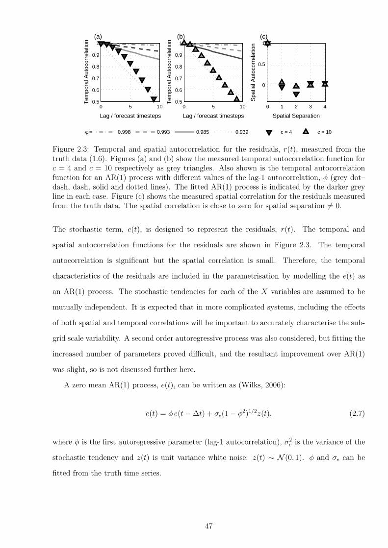
0 5 100.5
0.6
0.7
0.8
0.9
1
Lag / forecast timesteps
Tem
pora
l Aut
ocor
rela
tion
(a)
φ = 0.998 0.993 0.985 0.939
0 5 100.5
0.6
0.7
0.8
0.9
1
Lag / forecast timesteps
Tem
pora
l Aut
ocor
rela
tion
(b)
0 1 2 3 4
0
0.5
1
Spatial Separation
Spa
tial A
utoc
orre
latio
n
(c)
c = 4 c = 10
Figure 2.3: Temporal and spatial autocorrelation for the residuals, r(t), measured from thetruth data (1.6). Figures (a) and (b) show the measured temporal autocorrelation function forc = 4 and c = 10 respectively as grey triangles. Also shown is the temporal autocorrelationfunction for an AR(1) process with different values of the lag-1 autocorrelation, φ (grey dot–dash, dash, solid and dotted lines). The fitted AR(1) process is indicated by the darker greyline in each case. Figure (c) shows the measured spatial correlation for the residuals measuredfrom the truth data. The spatial correlation is close to zero for spatial separation 6= 0.
The stochastic term, e(t), is designed to represent the residuals, r(t). The temporal and
spatial autocorrelation functions for the residuals are shown in Figure 2.3. The temporal
autocorrelation is significant but the spatial correlation is small. Therefore, the temporal
characteristics of the residuals are included in the parametrisation by modelling the e(t) as
an AR(1) process. The stochastic tendencies for each of the X variables are assumed to be
mutually independent. It is expected that in more complicated systems, including the effects
of both spatial and temporal correlations will be important to accurately characterise the sub-
grid scale variability. A second order autoregressive process was also considered, but fitting the
increased number of parameters proved difficult, and the resultant improvement over AR(1)
was slight, so is not discussed further here.
A zero mean AR(1) process, e(t), can be written as (Wilks, 2006):
e(t) = φ e(t− ∆t) + σe(1 − φ2)1/2z(t), (2.7)
where φ is the first autoregressive parameter (lag-1 autocorrelation), σ2e is the variance of the
stochastic tendency and z(t) is unit variance white noise: z(t) ∼ N (0, 1). φ and σe can be
fitted from the truth time series.
47

2.3.2.2 State Dependent Noise (SD)
A second type of noise is considered where the standard deviation of additive noise is dependent
on the value of the X variable. This is called state dependent noise. It can be motivated in
the L96 system by studying Figure 2.2; the degree of scatter about the cubic fit is greater for
large magnitude X values. The parametrised tendency
Up = Udet + e(t), (2.8)
where the state dependent standard deviation of e(t) is modelled as
σe = σ1|X(t)| + σ0. (2.9)
As Figure 2.3 shows a large temporal autocorrelation, it is unlikely that white state dependent
noise will adequately model the residuals. Instead, e(t) will be modelled as an AR(1) process:
e(t) =σe(t)
σe(t− ∆t)φ e(t− ∆t) + σe(t)(1 − φ2)1/2z(t), (2.10)
where the time dependency of the standard deviation and the requirement that e(t) must be
a stationary process have motivated the functional form.
The parameters σ1 and σ0 can be estimated by binning the residuals according to the
magnitude of X and calculating the standard deviation in each bin. The lag-1 autocorrelation
was estimated from the residual time series.
2.3.2.3 Multiplicative Noise (M)
Multiplicative noise has been successfully implemented in the ECMWF NWP model using the
SPPT scheme, and has been shown to improve the skill of the forecasting system (Buizza et al.,
1999). Therefore it is of interest whether a parametrisation scheme involving multiplicative
noise could give significant improvements over additive stochastic schemes in the L96 system.
The parametrisation proposed is
Up = (1 + e(t))Udet, (2.11)
48

where e(t) is modelled as an AR(1) process, given by (2.7).
The parameters in this model can be estimated by forming a time series of the truth
“residual ratio”, Rk, that needs to be represented:
Rk + 1 = U /Udet. (2.12)
However whenever Udet approaches zero, the residual ratio tends to infinity. Therefore, the
time series was first filtered such that only sections away from Udet = 0 were considered, and
the temporal autocorrelation and standard deviation estimated from these sections.
For multiplicative noise, it is assumed that the standard deviation of the true tendency is
proportional to the parametrised tendency, such that when the parametrised tendency is zero
the uncertainty in the tendency is zero. Figure 2.2 shows that multiplicative noise does not
appear to be a good model for the uncertainty in the L96 system as the uncertainty in the true
tendency is large even when Udet is zero. In the case of the L96 system, the uncertainty when
Udet is zero is likely to be because the deterministic parametrisation has not fully captured
the behaviour of the Y variables. Time stepping errors may also contribute to this error.
Nevertheless, multiplicative noise is investigated here.
2.3.2.4 Multiplicative and Additive Noise (MA)
Figure 2.2 motivates a final stochastic parametrisation scheme for testing in the L96 system,
which will include both multiplicative and additive noise terms. This represents the uncertainty
in the parametrised tendency even when the deterministic tendency is zero. This type of
uncertainty has been observed in coarse-graining studies. For example, Shutts and Palmer
(2007) observed that the standard deviation of the true heating in a coarse gridbox does not
go to zero when Q, the parametrised heating, is zero. This type of stochastic parametrisation
can also be motivated by considering errors in the time stepping scheme, which will contribute
to errors in the total tendency even if the sub-grid scale tendency is zero.
When formulating this parametrisation, the following points were considered:
1. In a toy model setting, random number generation is computationally cheap. However in
a weather or climate prediction model, generation of spatially and temporally correlated
fields of random numbers is comparatively expensive, and two separate generators must
49

Full Name Abbreviation Functional FormMeasured Parameters
c = 4 c = 10
Additive AUp = Udet + e(t) φmeas = 0.993 φmeas = 0.986e(t) = φ e(t− ∆t) + σ(1 − φ2)1/2z(t) σmeas = 2.12 σmeas = 1.99
State Dependent SD
Up = Udet + e(t) φmeas = 0.993 φmeas = 0.989e(t) = σt
σt−∆tφ e(t− ∆t) + σt(1 − φ2)1/2z(t) (σ0)meas = 1.62 (σ0)meas = 1.47
where (σ1)meas = 0.078 (σ1)meas = 0.0873σt = σ1|X(t)| + σ0
Multiplicative MUp = (1 + e(t))Udet φmeas = 0.950 φmeas = 0.940e(t) = φ e(t− ∆t) + σ(1 − φ2)1/2z(t) σmeas = 0.746 σmeas = 0.469
Multiplicative & Additive MA
Up = Udet + e(t) φmeas = 0.993 φmeas = 0.988e(t) = ǫ(t) (σm|Udet| + σa) (σm)meas = 0.177 (σm)meas = 0.101where (σa)meas = 1.55 (σa)meas = 1.37ǫ(t) = ǫ(t− ∆t)φ+ (1 − φ2)1/2z(t)
Table 2.2: Stochastic parametrisations of the sub-grid tendency, U, used in this experiment, and the values of the model parameters fitted fromthe truth time series.
50
be used if two such fields are required. It is therefore desirable to use only one random
number per time step so that the parametrisation can be further developed for use in an
atmospheric model.
2. The fewer parameters there are to fit, the less complicated the methodology required to
fit them, the easier it will be to apply this method to a more complex system such as an
atmospheric model. This also avoids overfitting.
The most general form of additive and multiplicative noise is considered:
Up = (1 + ǫm)Udet + ǫa = Udet + (ǫm Udet + ǫa), (2.13)
where ǫm is the multiplicative noise term, and ǫa is the additive noise term. This can be written
as pure additive noise:
Up = Udet + e(t), (2.14)
where
e(t) = ǫm(t)Udet + ǫa(t). (2.15)
Following point (1) above, it is assumed that ǫm(t) and ǫa(t) are the same random number,
ǫ(t),
e(t) = ǫ(t) (σmUdet + σa) , (2.16)
where ǫ(t) has been scaled using the standard deviations of the multiplicative and additive
noise, σm and σa respectively. In the current form, (2.16) is not symmetric about the origin with
respect to Udet. The standard deviation of the stochastic tendency is zero when σmUdet = −σa.
Therefore, Udet in the above equation will be replaced with |Udet|:
e(t) = ǫ(t) (σm|Udet| + σa) , (2.17)
where
ǫ(t) = ǫ(t− ∆t)φ+ (1 − φ2)1/2z(t). (2.18)
This does not change the nature of the multiplicative noise as ǫ(t) has mean zero, but the
additive part of the noise will act in the same direction as the multiplicative. ǫ(t) is modelled
as a AR(1) process of unit variance. The parameters are fitted from the residual time series.
51

−1−0.8−0.6−0.4−0.200.1
0.3
0.3
φ
0.00
0
0.60
7
0.88
2
0.96
9
0.99
2
0.99
8
σ / σ
mea
s
(d) IGNSS, c = 10
0.0
0.5
1.0
1.5
2.0
2.50.70.720.740.76
0.78
0.8
0.8
0.82
φ
0.00
0
0.60
7
0.88
2
0.96
9
0.99
2
0.99
8
σ / σ
mea
s
(c) RPSS, c = 10
0.0
0.5
1.0
1.5
2.0
2.5
0.50.520.540.560.580.60.62
0.64
0.64
φ0.
000
0.60
7
0.88
2
0.96
9
0.99
3
0.99
8
σ / σ
mea
s
(a) RPSS, c = 4
0.0
0.5
1.0
1.5
2.0
2.5
−1−0.8−0.6−0.4−0.2
00.1
φ
0.00
0
0.60
7
0.88
2
0.96
9
0.99
3
0.99
8
σ / σ
mea
s
(b) IGNSS, c = 4
0.0
0.5
1.0
1.5
2.0
2.5
Figure 2.4: Weather Skill Scores (RPSS and IGNSS) for a forecast model with an additiveAR(1) stochastic parametrisation for (a) and (b) the c = 4 case, and (c) and (d) the c = 10case. The skill scores were evaluated as a function of the tuneable parameters in the model;the lag-1 autocorrelation, φ, and the standard deviation of the noise, σ. The black crossesindicate the measured parameter values. The contour interval is 0.01 for (a) and (c), and 0.1for (b) and (d). All skill scores are calculated at a lead time of 0.6 MTU (3 atmospheric days).
The possibility of using an additive and multiplicative noise scheme in the ECMWF NWP
model is discussed in Section 5.3.
The different stochastic parametrisations used in this experiment are summarised in Table
2.2, together with the parameters measured from the truth time series.
2.4 Weather Forecasting Skill
The stochastic parametrisation schemes are first tested on their ability to predict the “weather”
of the L96 system, and represent the uncertainty in their predictions correctly. An ensemble of
40 members is generated for each of the 300 initial conditions on the attractor. Each ensemble
member is initialised from the perfect initial conditions defined by the “truth” time series.
Each stochastic parametrisation involves two or more tunable parameters which may be
estimated from the “truth” time series. In addition to the measured parameter values, many
other parameter settings were considered, and the skill of the parametrisation evaluated for
each setting using three scalar skill scores. The RPS (Section 1.7.1.2) was evaluated for a
52

0.50.520.540.560.580.6
0.62
0.62
0.64
0.64
σ1 / (σ
1)meas
0.
0
0.
5
1.
0
1.
5
2.
0
2.
5
σ 0 / (σ
0) mea
s
(a) SD, c = 4
0.0
0.5
1.0
1.5
2.0
2.5
φ
0.00
0
0.60
7
0.88
2
0.96
9
0.99
3
0.99
8
σ / σ
mea
s
(b) M, c = 4
0.58
0.66
0.66
0.60.62
0.64
0.0
0.5
1.0
1.5
2.0
2.5 0.50.520.540.560.580.60.620.64
σm
/ (σm
)meas
0.
0
0.
5
1.
0
1.
5
2.
0
2.
5
σ a / (σ
a) mea
s
(c) AR1 MA, c = 4
0.0
0.5
1.0
1.5
2.0
2.5
0.70.720.740.760.780.8
0.82
0.82
σ1 / (σ
1)meas
0.
0
0.
5
1.
0
1.
5
2.
0
2.
5
σ 0 / (σ
0) mea
s
(d) AR(1) SD, c = 10
0.0
0.5
1.0
1.5
2.0
2.5
φ
0.00
0
0.60
7
0.88
2
0.96
9
0.99
2
0.99
8
σ / σ
mea
s
(e) M, c = 10
0.80.82
0.820.8
0.760.72
0.0
0.5
1.0
1.5
2.0
2.50.720.74
0.760.78
0.8
0.820.82
0.82
σm
/ (σm
)meas
0.
0
0.
5
1.
0
1.
5
2.
0
2.
5
σ a / (σ
a) mea
s
(f) AR(1) MA, c = 10
0.0
0.5
1.0
1.5
2.0
2.5
Figure 2.5: Comparing the RPSS for the c = 4 and c = 10 cases for the different stochasticparametrisations. For c = 4, (a) the skill of the state dependant (SD) additive parametrisa-tion is shown for different values of the noise standard deviations, σ1 and σ0, with the lag-1autocorrelation set to φ = φmeas. (b) The skill of the pure multiplicative (M) noise is shownfor different values of the lag-1 autocorrelation, φ, and magnitude of the noise, σ. The para-metrisation scheme was found to be numerically unstable for high σ > 2σmeas. (c) The skillof the additive and multiplicative (MA) parametrisation is shown for different values of thenoise standard deviations, σm and σa, with the lag-1 autocorrelation set to φ = φmeas. Theequivalent figures for c = 10 are shown in (d)–(f). In all cases, the measured parameters areindicated by the black cross. The contour interval is 0.01 for each case. The skill scores wereevaluated at a lead time of 0.6 model time units (3 atmospheric days).
ten-category forecast, where the categories were defined as the ten deciles of the climatological
distribution. IGN (Section 1.7.1.3) was evaluated using the method suggested by Roulston
and Smith (2002). The BS (Section 1.7.1.1) was evaluated for the event “the X variable is in
the upper tercile of the climatological distribution”. The BS is mathematically related to the
RPS (Wilks, 2006), and gave very similar results to the RPS, so is not shown here for brevity.
A skill score was calculated for each score with respect to climatology. Forecasts were verified
at a lead time of 0.6 units, equivalent to 3 atmospheric days.
Figure 2.4 shows the calculated skill scores for a forecast model with an additive AR(1)
stochastic parametrisation, for both the c = 4 and c = 10 cases. There is a broad peak in
forecasting skill according to each skill score, with a range of parameter settings scoring highly.
The shape of peak in forecasting skill is qualitatively similar in each case, but is lower for the
53
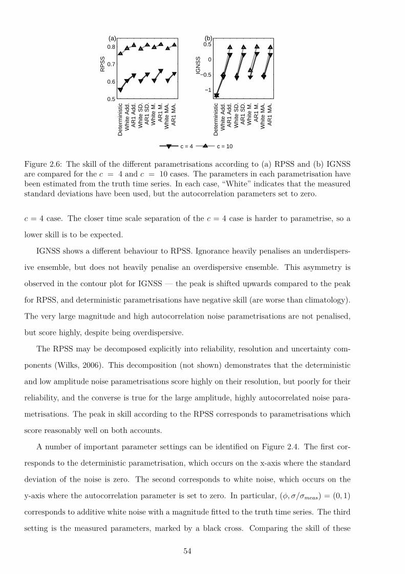
0.5
0.6
0.7
0.8
RP
SS
(a)
Det
erm
inis
ticW
hite
Add
.A
R1
Add
.W
hite
SD
.A
R1
SD
.W
hite
M.
AR
1 M
.W
hite
MA
.A
R1
MA
.
c = 4 c = 10
−1
−0.5
0
0.5
IGN
SS
(b)
Det
erm
inis
ticW
hite
Add
.A
R1
Add
.W
hite
SD
.A
R1
SD
.W
hite
M.
AR
1 M
.W
hite
MA
.A
R1
MA
.
Figure 2.6: The skill of the different parametrisations according to (a) RPSS and (b) IGNSSare compared for the c = 4 and c = 10 cases. The parameters in each parametrisation havebeen estimated from the truth time series. In each case, “White” indicates that the measuredstandard deviations have been used, but the autocorrelation parameters set to zero.
c = 4 case. The closer time scale separation of the c = 4 case is harder to parametrise, so a
lower skill is to be expected.
IGNSS shows a different behaviour to RPSS. Ignorance heavily penalises an underdispers-
ive ensemble, but does not heavily penalise an overdispersive ensemble. This asymmetry is
observed in the contour plot for IGNSS — the peak is shifted upwards compared to the peak
for RPSS, and deterministic parametrisations have negative skill (are worse than climatology).
The very large magnitude and high autocorrelation noise parametrisations are not penalised,
but score highly, despite being overdispersive.
The RPSS may be decomposed explicitly into reliability, resolution and uncertainty com-
ponents (Wilks, 2006). This decomposition (not shown) demonstrates that the deterministic
and low amplitude noise parametrisations score highly on their resolution, but poorly for their
reliability, and the converse is true for the large amplitude, highly autocorrelated noise para-
metrisations. The peak in skill according to the RPSS corresponds to parametrisations which
score reasonably well on both accounts.
A number of important parameter settings can be identified on Figure 2.4. The first cor-
responds to the deterministic parametrisation, which occurs on the x-axis where the standard
deviation of the noise is zero. The second corresponds to white noise, which occurs on the
y-axis where the autocorrelation parameter is set to zero. In particular, (φ, σ/σmeas) = (0, 1)
corresponds to additive white noise with a magnitude fitted to the truth time series. The third
setting is the measured parameters, marked by a black cross. Comparing the skill of these
54

three cases shows an improvement over the deterministic scheme as first white noise, then red
noise is included in the parametrisation.
The RPSS calculated for the other stochastic parametrisation schemes is shown in Fig-
ure 2.5. The contour plots for IGNSS are comparable, so are not shown for brevity. The
forecasts are more skilful for the c = 10 case, but qualitatively similar. This result is as ex-
pected: the closer time scale separation for the c = 4 case is harder to parametrise, so the
forecast models perform less well than for the c = 10 case. For both cases considered, for all
parametrisation schemes, including a stochastic term in the parametrisation scheme results in
an improvement in the skill of the forecast over the deterministic scheme. This result is robust
to error in the measurement of the parameters — a range of parameters in each forecast model
gave good skill scores. This is encouraging, as it indicates that stochastic parametrisations
could be useful in modelling the real atmosphere, where noisy data restrict how accurately
these parameters may be estimated.
The results are summarised in Figure 2.6. For each parametrisation, the value for the
measured parameters is shown when both no temporal autocorrelation (“white” noise) and
the measured temporal autocorrelation characteristics are used. The significance of the dif-
ference between pairs of parametrisations was estimated using a Monte-Carlo technique. See
Appendix A for more details. For example, there is no significant difference between the RPS
for AR(1) MA noise and for AR(1) SD noise for the c = 10 case, but AR(1) M noise gave a
significant improvement over both of these.
The stochastic parametrisations are significantly more skilful than the deterministic para-
metrisation in both the c = 4 and c = 10 cases. For the c = 4 case, the more complicated
parametrisations show a significant improvement over simple additive noise, especially the mul-
tiplicative noise. For the closer time scale separation, the more accurate the representation of
the sub-grid scale forcing, the higher the forecast skill. For the c = 10 case, the large time
scale separation allows the deterministic parametrisation to have reasonable forecasting skill,
and a simple representation of sub-grid variability is sufficient to represent the uncertainty in
the forecast model; the more complicated stochastic parametrisations show little improvement
over simple additive AR(1) noise.
Traditional deterministic parametrisation schemes are a function of the grid scale variables
at the current time step only. If a stochastic parametrisation needs only to represent the sub
55
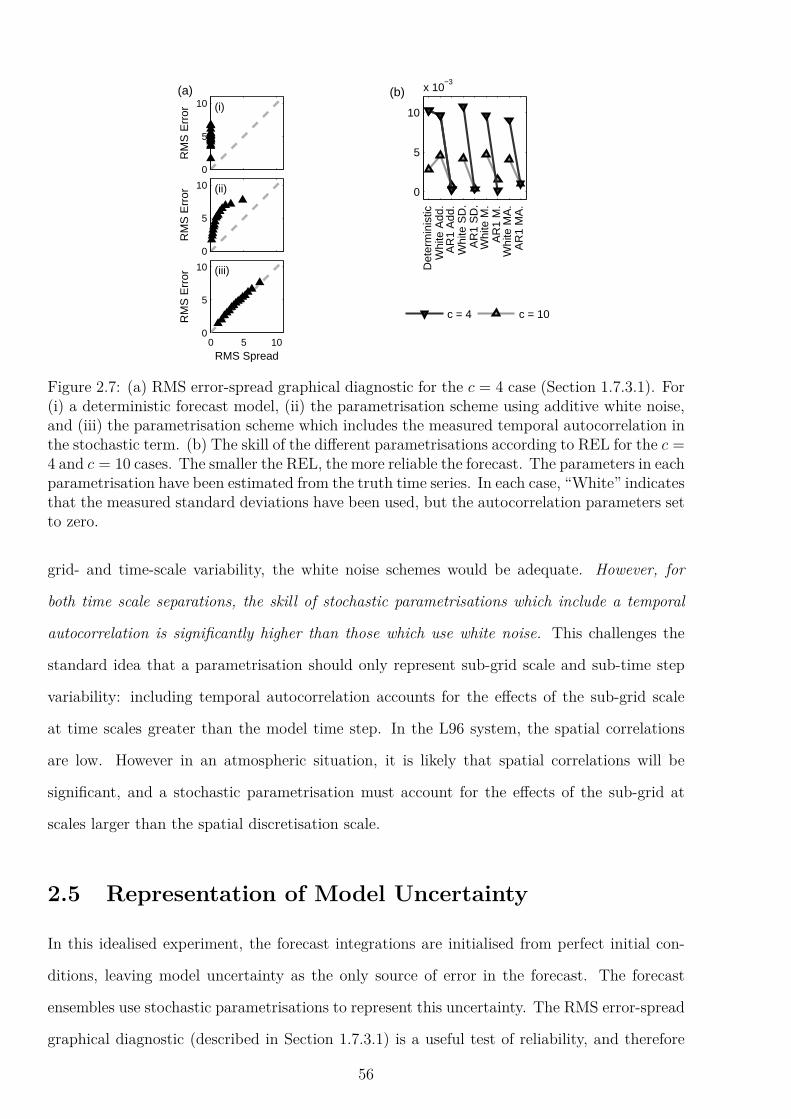
0
5
10
RM
S E
rror (i)
(a)
0
5
10R
MS
Err
or (ii)
0 5 100
5
10
RMS Spread
RM
S E
rror (iii)
0
5
10
x 10−3
Det
erm
inis
ticW
hite
Add
.A
R1
Add
.W
hite
SD
.A
R1
SD
.W
hite
M.
AR
1 M
.W
hite
MA
.A
R1
MA
.
(b)
c = 4 c = 10
Figure 2.7: (a) RMS error-spread graphical diagnostic for the c = 4 case (Section 1.7.3.1). For(i) a deterministic forecast model, (ii) the parametrisation scheme using additive white noise,and (iii) the parametrisation scheme which includes the measured temporal autocorrelation inthe stochastic term. (b) The skill of the different parametrisations according to REL for the c =4 and c = 10 cases. The smaller the REL, the more reliable the forecast. The parameters in eachparametrisation have been estimated from the truth time series. In each case, “White” indicatesthat the measured standard deviations have been used, but the autocorrelation parameters setto zero.
grid- and time-scale variability, the white noise schemes would be adequate. However, for
both time scale separations, the skill of stochastic parametrisations which include a temporal
autocorrelation is significantly higher than those which use white noise. This challenges the
standard idea that a parametrisation should only represent sub-grid scale and sub-time step
variability: including temporal autocorrelation accounts for the effects of the sub-grid scale
at time scales greater than the model time step. In the L96 system, the spatial correlations
are low. However in an atmospheric situation, it is likely that spatial correlations will be
significant, and a stochastic parametrisation must account for the effects of the sub-grid at
scales larger than the spatial discretisation scale.
2.5 Representation of Model Uncertainty
In this idealised experiment, the forecast integrations are initialised from perfect initial con-
ditions, leaving model uncertainty as the only source of error in the forecast. The forecast
ensembles use stochastic parametrisations to represent this uncertainty. The RMS error-spread
graphical diagnostic (described in Section 1.7.3.1) is a useful test of reliability, and therefore
56

a good indicator of how well the forecast model represents uncertainty. Figure 2.7(a) shows
this diagnostic for a selection of the parametrisation schemes tested for the c = 4 case. For a
well calibrated ensemble, the points should lie on the diagonal. A clear improvement over the
deterministic scheme is seen as first white, then red additive noise is included in the paramet-
risation scheme.
Visual forecast verification measures are limited when comparing many different models as
they do not give an unambiguous ranking of the performance of these models. Therefore, the
reliability component of the Brier Score (1.17), REL, is also considered. This is a scalar scoring
rule which tests the reliability of an ensemble forecast at predicting an event. The event is
defined to be “in the upper tercile of the climatological distribution”. The smaller the REL,
the closer the forecast probability is to the average observed frequency, the more reliable the
forecast.
The results are summarised in Figure 2.7(b). The REL score indicates that the different
AR(1) noise terms all perform similarly. A significant improvement is observed when tem-
poral autocorrelation is included in the parametrisation, particularly for the c = 4 case. This
improvement between white and red stochastic models is much greater than the difference
between deterministic and white stochastic models, whereas the RPSS indicated a similar im-
provement as first white then red noise schemes were tested. This indicates that while overall
forecast skill can be improved to a reasonable extent using a white noise stochastic scheme, for
reliable forecasts it is very important that the stochastic parametrisation includes temporally
correlated noise as this captures the behaviour of the unresolved sub-grid scale variables better.
2.6 Perturbed Parameter Ensembles in the Lorenz ’96
System
It is of interest to determine whether a perturbed parameter ensemble can also provide a
reliable measure of model uncertainty in the Lorenz ’96 system. The four measured parameters
(bmeas0 , bmeas
1 , bmeas2 , bmeas
3 ) defining the cubic polynomial are perturbed to generate a 40 member
ensemble. The skill of this representation of model uncertainty is evaluated as for the stochastic
parametrisations.
Following Stainforth et al. (2005), each of the four parameters is set to one of three values:
57

−15 −10 −5 0 5 10 15 20−20
−10
0
10
20
X
Sub
grid
Ten
denc
y, U
Udet
= − 0.000223 X3 − 0.00550 X2
+ 0.575 X − 0.198
(a)
−10 −5 0 5 10 15−20
−10
0
10
20
XS
ubgr
id T
ende
ncy,
U
Udet
= − 0.00235 X3 − 0.0136 X2
+ 1.30 X + 0.341
(b)
Figure 2.8: The ensemble of deterministic parametrisations used to represent model uncertaintyin the perturbed parameter ensemble (solid lines), compared to the measured sub-grid tendency,U , as a function of the grid scale variables, X (circles), for both the (a) c = 4 and (b) c = 10cases. The degree to which the parameters are perturbed has been estimated from the truthtime series in each case (S = 1).
c = 4 c = 10
bmeas0 -0.198 0.341σ(bsamp
0 ) 0.170 0.146bmeas
1 0.575 1.30σ(bsamp
1 ) 0.0464 0.0381bmeas
2 -0.00550 -0.136σ(bsamp
2 ) 0.00489 0.00901bmeas
3 -0.000223 -0.00235σ(bsamp
3 ) 0.000379 0.000650
Table 2.3: Measured parameters defining the cubic polynomial, (bmeas0 , bmeas
1 , bmeas2 , bmeas
3 ), andthe variability of these parameters, σ(bsamp
i ), calculated by sampling from the truth time series,for the c = 4 and c = 10 cases.
58

low (L), medium (M) or high (H). The degree to which the parameters should be varied
is estimated from the truth time series. The measured U(X) is split into sections 3 MTU
long, and a cubic polynomial fitted to each section. The measured variability in each of the
parameters is defined to be the standard deviation of the parameters fitted to each section
σ(bsampi ). The measured standard deviations are shown in Table 2.3. The low, medium and
high values of the parameters are given by:
L = bmeasi − Sσ(bsamp
i )
M = bmeasi
H = bmeasi + Sσ(bsamp
i ), (2.19)
where the scale factor, S, can be varied to test the sensitivity of the scheme. There are 34 = 81
possible permutations of the parameter settings, from which a subset of 40 permutations was
selected to sample the uncertainty. This allows for a fair comparison to be made with the
stochastic parametrisations, which also use a 40 member ensemble. The selected permutations
are shown in Table 2.4.
The same “truth” model is used as for the stochastic parametrisations, and the forecast
model is constructed in an analogous way: only the X variables are assumed resolved, and
the effects of the unresolved sub-grid scale Y variables are represented by an ensemble of
deterministic parametrisations:
Upp(Xk) = bp0 + bp
1Xk + bp2X
2k + bp
3X3k , (2.20)
where the values of the perturbed parameters, bpi , vary between ensemble members. The
scale factor, S, in (2.19) is varied to investigate the effect on the skill of the forecast. The
ensemble of deterministic parametrisations is shown in Figure 2.8 where the degree of parameter
perturbation has been measured from the truth time series (i.e. S = 1). The truncated model
is integrated using an adaptive second order Runge-Kutta scheme.
2.6.1 Weather Prediction Skill
The skill of the ensemble forecast is evaluated using the RPSS and IGNSS at a lead time of
0.6 model time units for both the c = 4 and c = 10 cases. The results are shown in Figure 2.9.
59

Selected PermutationsNumber b0 b1 b2 b3 Number b0 b1 b2 b3
1 H H H H 21 M M L H2 H H H L 22 M M L L3 H H M M 23 M L H M4 H H L H 24 M L M H5 H H L L 25 M L M L6 H M H M 26 M L L M7 H M M H 27 L H H H8 H M M L 28 L H H L9 H M L M 29 L H M M10 H L H H 30 L H L H11 H L H L 31 L H L L12 H L M M 32 L M H M13 H L L H 33 L M M H14 H L L L 34 L M M L15 M H H M 35 L M L M16 M H M H 36 L L H H17 M H M L 37 L L H L18 M H L M 38 L L M M19 M M H H 39 L L L H20 M M H L 40 L L L L
Table 2.4: Chosen permutations for the perturbed parameter experiment. H, M and L representthe High, Medium and Low settings respectively.
Scale Factor, S
(d) RPSS, c = 10
0.78
0.80
0.82
0.0 0.2 0.4 0.6 0.8 1.0 1.2 1.4 1.6 1.8 2.0
Scale Factor, S
(e) IGNSS, c = 10
−1
−0.
8
−0.
6
−0.
4
−0.
2
0 0.1
0.0 0.2 0.4 0.6 0.8 1.0 1.2 1.4 1.6 1.8 2.0
Scale Factor, S
(f) REL, c = 10
0.00
3
0.00
1
0.0 0.2 0.4 0.6 0.8 1.0 1.2 1.4 1.6 1.8 2.0
0.56
0.58
0.6 0.
62
0.64
0.66
0.68
Scale Factor, S
(a) RPSS, c = 4
0.0 0.2 0.4 0.6 0.8 1.0 1.2 1.4 1.6 1.8 2.0 2.2 2.4 2.6
−1
−1
−0.
8
−0.
6
−0.
4
−0.
2
00
0.1
Scale Factor, S
(b) IGNSS, c = 4
0.0 0.2 0.4 0.6 0.8 1.0 1.2 1.4 1.6 1.8 2.0 2.2 2.4 2.6
Scale Factor, S
(c) REL, c = 4
0.00
9
0.00
5
0.0 0.2 0.4 0.6 0.8 1.0 1.2 1.4 1.6 1.8 2.0 2.2 2.4 2.6
Figure 2.9: Weather forecasting skill scores for the perturbed parameter model as a functionof the scale factor, S. The skill of the c = 4 forecasts according to (a) RPSS, (b) IGNSS and(c) REL. The equivalent results for c = 10 are shown in (d)–(f). The contour interval is 0.01in (a) and (d), 0.1 in (b) and (e), and 0.001 in (c) and (f). The skill scores are calculated at alead time of 0.6 MTU in each case.
60

0 50
5
RM
S E
rror
RMS Spread0 5
0
5
RMS Spread0 5
0
5
RMS Spread
(b) c = 10
0 50
5
RMS Spread0 5
0
5
RMS Spread0 5
0
5
RMS Spread
0 5 100
5
10
RM
S E
rror
RMS Spread0 5 10
0
5
10
RMS Spread0 5 10
0
5
10
RMS Spread
(a) c = 4
0 5 100
5
10
RMS Spread0 5 10
0
5
10
RMS Spread0 5 10
0
5
10
RMS Spread
Increasing s
Increasing s
Figure 2.10: RMS Spread vs. RMS Error plots for the perturbed parameter ensemble as a func-tion of the scale factor, S. The separate figures correspond to S = [0.0, 0.4, 0.8, 1.2, 1.6, 2.0].
The measured parameter perturbations are indicated with a black cross in each case.
Both RPSS and IGNSS indicate that the measured perturbed parameter ensemble is signific-
antly less skilful than the stochastic ensemble for both the c = 4 and c = 10 case. Figures 2.9(c)
and (f) show the reliability component of the Brier Score calculated for the perturbed para-
meter ensembles. Comparing these figures with Figure 2.7(b), REL for the perturbed parameter
schemes is greater, indicating that the perturbed parameter ensemble forecasts are less reliable
than the stochastic parametrisation forecasts, and the ensemble is a poorer representation of
model uncertainty. The significance of the difference between skill scores for the measured
stochastic parametrisation schemes and the perturbed parameter schemes with the measured
perturbations (S = 1) are shown in Appendix A.
The reliability of the forecast ensemble is also considered using the RMS error-spread
diagnostic as a function of the scale factor (Figure 2.10). For small-scale factors, the ensemble
is systematically underdispersive for both the c = 4 and c = 10 cases. For larger scale
factors for the c = 10 case, the ensemble is systematically overdispersive for large errors,
and underdispersive for small errors. Comparing Figure 2.10 with Figure 2.7(a) shows that
none of the perturbed parameter ensembles are as reliable as the AR(1) additive stochastic
parametrisation, reflected in the poorer REL score for the perturbed parameter case.
61

2.7 Conclusion
Several different stochastic parametrisation schemes were investigated using the Lorenz ’96
(L96) system. All showed an improvement in weather forecasting skill over deterministic
parametrisations. This result is robust to error in measurement of the parameters — scanning
over parameter space indicated a wide range of parameter settings gave good skill scores.
Importantly, stochastic parametrisations have been shown to represent the uncertainty in a
forecast due to model deficiencies accurately, as demonstrated by an increase in the reliability
of the forecasts.
A significant improvement in the skill of the forecast models was observed when the
stochastic parametrisations included temporal autocorrelation in the noise term. This chal-
lenges the notion that a parametrisation scheme should only represent sub-grid scale (both
temporal and spatial) variability. The coupling of scales in a complex system means a success-
ful parametrisation must represent the effects of the sub-grid scale processes acting on spatial
and time scales greater than the truncation level.
Stochastic representations of model uncertainty are shown to outperform perturbed para-
meter ensembles in the L96 system. They have improved short term forecasting skill and are
more reliable than perturbed parameter ensembles.
The L96 system is an excellent tool for testing developments in stochastic parametrisations.
These ideas can now be applied to numerical weather prediction models and tested on the
atmosphere.
62

3
The Lorenz ’96 System:
Climatology and Regime Behaviour
I believe that the ultimate climatic models ... will be stochastic, i.e., random numbers
will appear somewhere in the time derivatives.
– Ed Lorenz, 1975
3.1 Introduction
There is no formal definition of climate. The climate of a region can be defined in terms of the
long term statistics of weather in that region, including both the mean and the variability. The
World Meteorological Organisation defines thirty years as a suitable period of time for calculat-
ing these statistics. The calculated “climate” will be sensitive to this selected period, especially
if the climate is not stationary. Lorenz (1997) proposes several definitions of climate motivated
by dynamical systems theory, including suggesting that “the climate [can be identified as] the
attractor of the dynamical system”. Whereas weather forecasting is considered to be an initial
value problem, climate is often considered to be a boundary condition problem (Bryson, 1997),
with climate change occurring in response to changes in the boundary conditions.
As well as being difficult to define, it is difficult to verify climate projections. Probabilistic
weather forecasts can be verified since many forecast-observation pairs are available to test the
statistics of the forecast. This is not possible for climate predictions as there is only one evolu-
tion of the climate, and we must wait many years for new data to become available. However,
63
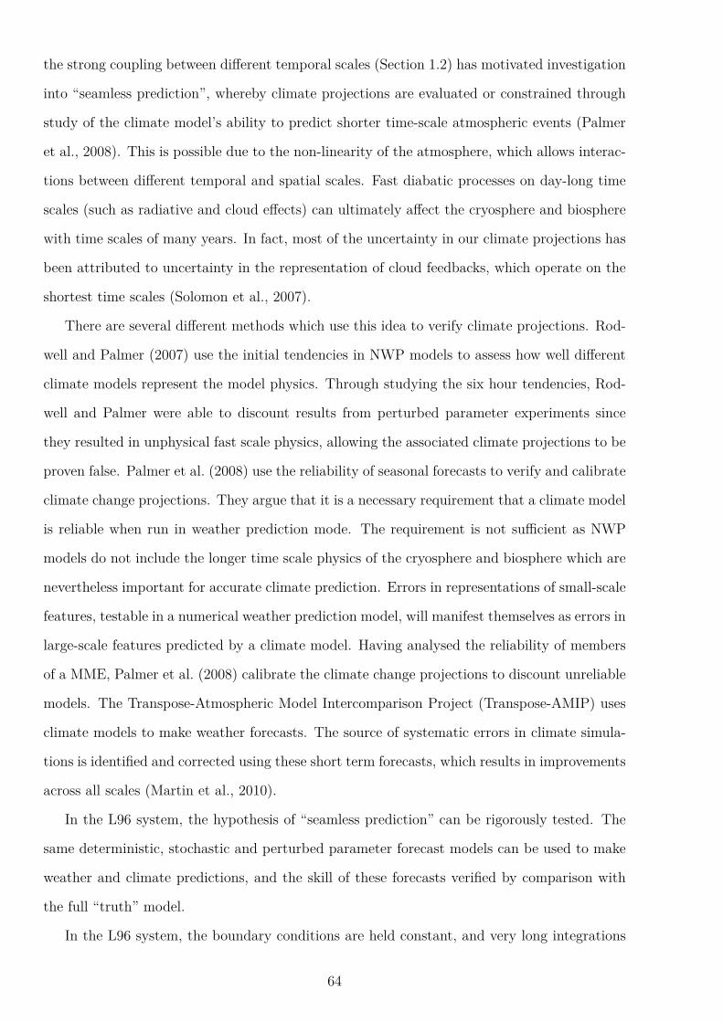
the strong coupling between different temporal scales (Section 1.2) has motivated investigation
into “seamless prediction”, whereby climate projections are evaluated or constrained through
study of the climate model’s ability to predict shorter time-scale atmospheric events (Palmer
et al., 2008). This is possible due to the non-linearity of the atmosphere, which allows interac-
tions between different temporal and spatial scales. Fast diabatic processes on day-long time
scales (such as radiative and cloud effects) can ultimately affect the cryosphere and biosphere
with time scales of many years. In fact, most of the uncertainty in our climate projections has
been attributed to uncertainty in the representation of cloud feedbacks, which operate on the
shortest time scales (Solomon et al., 2007).
There are several different methods which use this idea to verify climate projections. Rod-
well and Palmer (2007) use the initial tendencies in NWP models to assess how well different
climate models represent the model physics. Through studying the six hour tendencies, Rod-
well and Palmer were able to discount results from perturbed parameter experiments since
they resulted in unphysical fast scale physics, allowing the associated climate projections to be
proven false. Palmer et al. (2008) use the reliability of seasonal forecasts to verify and calibrate
climate change projections. They argue that it is a necessary requirement that a climate model
is reliable when run in weather prediction mode. The requirement is not sufficient as NWP
models do not include the longer time scale physics of the cryosphere and biosphere which are
nevertheless important for accurate climate prediction. Errors in representations of small-scale
features, testable in a numerical weather prediction model, will manifest themselves as errors in
large-scale features predicted by a climate model. Having analysed the reliability of members
of a MME, Palmer et al. (2008) calibrate the climate change projections to discount unreliable
models. The Transpose-Atmospheric Model Intercomparison Project (Transpose-AMIP) uses
climate models to make weather forecasts. The source of systematic errors in climate simula-
tions is identified and corrected using these short term forecasts, which results in improvements
across all scales (Martin et al., 2010).
In the L96 system, the hypothesis of “seamless prediction” can be rigorously tested. The
same deterministic, stochastic and perturbed parameter forecast models can be used to make
weather and climate predictions, and the skill of these forecasts verified by comparison with
the full “truth” model.
In the L96 system, the boundary conditions are held constant, and very long integrations
64

can be used to define the climate. We consider two definitions of “climate” in the L96 system.
The first is that the climate of L96 can be described as the pdf of the X variables calculated
over a sufficiently long time window. This will include information about both the mean and
the variability, as required for the conventional definition of climate outlined above. The second
definition will consider the presence and predictability of regime behaviour in the L96 system.
This is a dynamics-driven definition of climate as it includes information about the temporal
statistics of weather. It uncovers some of the characteristics of the system’s attractor, following
Lorenz’s definition of climate given above.
In Section 3.2, the forecast models outlined in Chapter 2 are evaluated according to their
skill at reproducing the pdf of the atmosphere. The “seamless prediction” hypothesis is tested
by comparing the climatological skill with the weather prediction skill, evaluated in Chapter 2.
In Section 3.3, atmospheric regime behaviour is introduced, and a subset of the L96 forecast
models are tested on their ability to reproduce the regime behaviour of the L96 system. For
each definition of climate, the performance of stochastic and perturbed parameter models will
be compared with the results from the full “truth” system.
3.2 Climatological Skill: Reproducing the pdf of the At-
mosphere
The climatology of the L96 system is defined to be the pdf of the X variables, averaged over
a long run (10,000 model time units ∼ 140 “atmospheric years”), and the forecast climatology
is defined in an analogous way. The skill at predicting the climatology can then be quantified
by measuring the difference between these two pdfs, which may be evaluated in several ways.
The Kolmogorov-Smirnov (KS) statistic, Dks, has been used in this context in several other
studies (Wilks, 2005; Kwasniok, 2012), where
Dks = maxXk
|P (Xk) −Q(Xk)| . (3.1)
65
0.004
0.006
0.008
0.004
φ
0.00
0
0.60
7
0.88
2
0.96
9
0.99
2
0.99
8
σ / σ
mea
s
(d) KL. Divergence, c = 10
0.0
0.5
1.0
1.5
2.0
2.5
0.03
0.038
φ
0.00
0
0.60
7
0.88
2
0.96
9
0.99
2
0.99
8
σ / σ
mea
s
(c) Hellinger Distance, c = 10
0.0
0.5
1.0
1.5
2.0
2.5
0.038
0.042
φ0.
000
0.60
7
0.88
2
0.96
9
0.99
3
0.99
8
σ / σ
mea
s
(a) Hellinger Distance, c = 4
0.034
0.0
0.5
1.0
1.5
2.0
2.5
0.006
0.008
φ
0.00
0
0.60
7
0.88
2
0.96
9
0.99
3
0.99
8
σ / σ
mea
s
(b) KL. Divergence, c = 4
0.0
0.5
1.0
1.5
2.0
2.5
Figure 3.1: Comparing the Hellinger distance and the Kullback-Leibler divergence as measuresof climatological skill. The measures are shown for the additive AR(1) noise parametrisation,as a function of the tuneable parameters, for both (a) and (b) the c = 4 case, and (c) and (d)the c = 10 case. The crosses indicate the measured parameters.
Here P is the forecast cumulative pdf, and Q is the verification cumulative pdf. A second
measure, the Hellinger distance, DHell, was also calculated for each forecast model:
D2Hell(p, q) =
1
2
∫ (√
p(x) −√
q(x))2
dx, (3.2)
where p(x) is the forecast pdf, and q(x) is the verification pdf (Pollard, 2002). Similarly, the
Kullback-Leibler (KL) divergence (Dkl), is defined as
Dkl(p, q) =∫
p(x)ln
(
p(x)
q(x)
)
dx. (3.3)
This measure is motivated by information theory (Kullback and Leibler, 1951), and is equi-
valent to the relative entropy between the two distributions (Section 1.7.1.3). For all these
measures, the smaller the measure, the better the match between forecast and verification
climatologies.
The Hellinger distance was found to be a much smoother measure of climatological skill
than the KS statistic as it integrates over the whole pdf. Therefore, the KS statistic has
66

0.03
0.038
σ1 / (σ
1)meas
0
.0
0
.5
1
.0
1
.5
2
.0
2
.5
σ 0 / (σ
0) mea
s
(a) AR1 SD, c = 4
0.0
0.5
1.0
1.5
2.0
2.5
0.03
0.038
φ
0.00
0
0.60
7
0.88
2
0.96
9
0.99
3
0.99
8
σ / σ
mea
s
(b) M, c = 4
0.0
0.5
1.0
1.5
2.0
2.5
0.03
0.038
σm
/ (σm
)meas
0
.0
0
.5
1
.0
1
.5
2
.0
2
.5
σ a / (σ
a) mea
s
(c) AR1 MA, c = 4
0.0
0.5
1.0
1.5
2.0
2.5
0.03
0.038
σ1 / (σ
1)meas
0
.0
0
.5
1
.0
1
.5
2
.0
2
.5
σ 0 / (σ
0) mea
s
(a) AR(1) SD, c = 10
0.034
0.034
0.0
0.5
1.0
1.5
2.0
2.5
φ
0.00
0
0.60
7
0.88
2
0.96
9
0.99
3
0.99
8
σ / σ
mea
s
(b) M, c = 10
0.038
0.03
0.034
0.0
0.5
1.0
1.5
2.0
2.5
0.03
0.03
σm
/ (σm
)meas
0
.0
0
.5
1
.0
1
.5
2
.0
2
.5
σ a / (σ
a) mea
s
(c) AR(1) MA, c = 10
0.0
0.5
1.0
1.5
2.0
2.5
Figure 3.2: The climatological skill of different stochastic parametrisations for the c = 4 andc = 10 cases, as a function of the tuneable parameters in each parametrisation. The crossesindicate the measured parameters in each case. For the SD and MA cases, φ is set to φmeas. TheHellinger distance was calculated between the truth and forecast probability density function(pdf) of the X variables. The smaller the Hellinger distance, the better the forecast pdf.
not been considered further here. Figure 3.1 shows that the Hellinger distance and Kullback-
Leibler divergence give very similar results, so for these reasons only the Hellinger distance will
be considered. Pollard (2002) shows that the two measures are linked, so this similarity is not
surprising.
The Hellinger distance is evaluated for the different stochastic parametrisations for the two
cases, c = 4 and c = 10. Figures 3.1 and 3.2 shows the results for c = 4 and c = 10 when the
tuneable parameters were varied as for the weather skill scores (Section 2.4). The climatology
of the c = 10 case is more skilful than for the c = 4 case, as indicated by smaller Hellinger
distances. The larger time scale separation for the c = 10 case is easier to parametrise, so the
forecast models perform better than for the c = 4 case. The peak of skill is shifted for the c = 4
case compared to the c = 10 case, towards parametrisation schemes with larger magnitude
noise. Qualitatively, the shape of the plots is similar to those for the equivalent weather skill
scores. This suggests that if a parametrisation performs well in weather forecasting mode, it
performs well at simulating the climate. The peak is shifted up and to the right compared to
the RPSS, but is in a similar position to IGNSS and REL.
67

0.03
0.035
0.04
0.045
Hel
linge
r D
ista
nce
Det
erm
inis
ticW
hite
Add
.A
R1
Add
.W
hite
SD
.A
R1
SD
.W
hite
M.
AR
1 M
.W
hite
MA
.A
R1
MA
.
c = 4 c = 10
Figure 3.3: The Hellinger distance for the different parametrisations is compared for the c = 4and c = 10 cases. The smaller the Hellinger distance, the better the climatological “skill”.The parameters in each parametrisation have been estimated from the truth time series. Ineach case, “White” indicates that the measured standard deviations have been used, but theautocorrelation parameters set to zero.
The climatological skill for the different parametrisations is summarised in Figure 3.3. As
for the weather forecasting skill, a significant improvement in the climatological skill is observed
when temporal autocorrelation is included in the parametrisations. This is demonstrated in
Appendix A.2, which shows the significance of the difference between the parametrisation
schemes tested when white or red noise is used. The white noise climatologies do not show a
significant improvement over the deterministic climatology for both the c = 4 and c = 10 case.
The red noise schemes are all significantly better than both the deterministic and white noise
stochastic parametrisation schemes, with the red multiplicative scheme performing significantly
better than all schemes for both the c = 4 and c = 10 case.
The climatological skill, as measured by the Hellinger distance, can be compared to the
weather skill scores using scatter diagrams (Figure 3.4). This is of interest, as the seamless
prediction paradigm suggests that climate models could be verified by evaluating the model in
weather forecasting mode. Figures 3.4(a) and 3.4(d) show the relationship between RPSS and
the Hellinger distance. For the c = 10 case, there appears to be a strong negative correlation
between the two. However, the peak in RPSS is offset slightly from the minimum in Hellinger
distance giving two branches in the scatter plot. The c = 4 case can be interpreted as being
positioned at the joining point of the two branches, and shows how using the RPSS as a method
to verify a model’s climatological skill could be misleading.
Figures 3.4(b) and 3.4(e) compare IGNSS with the Hellinger distance. The upper branch in
68
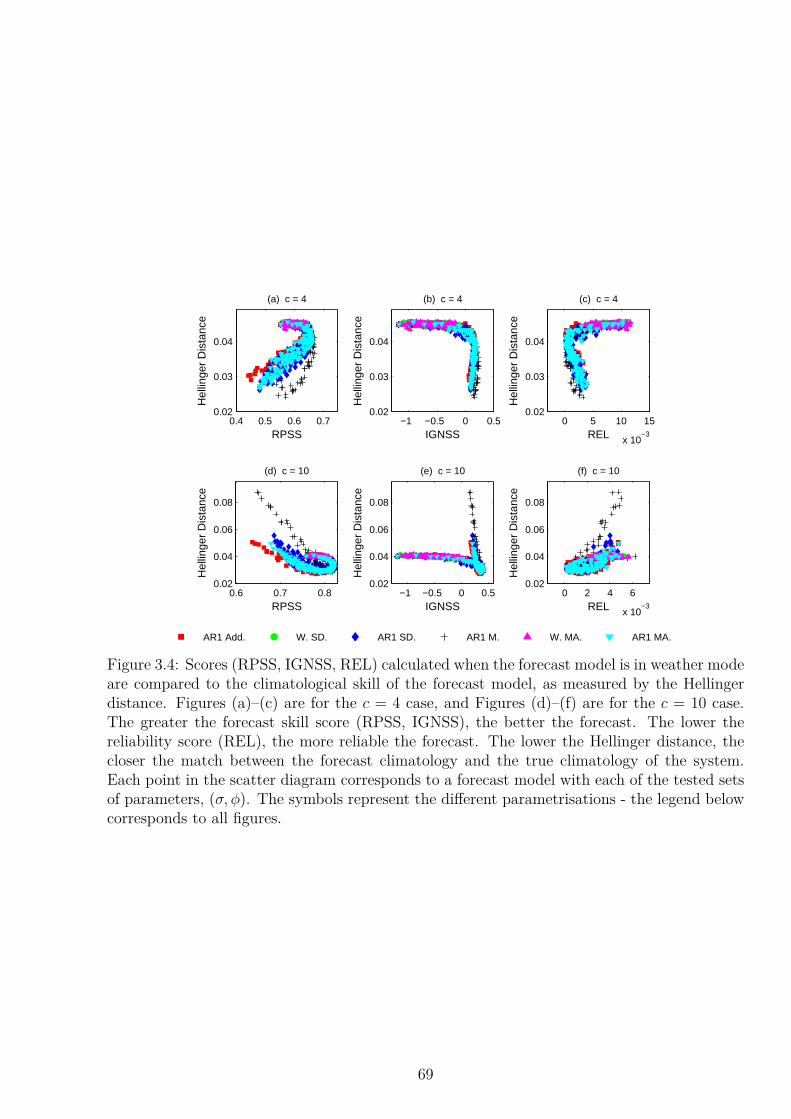
0.6 0.7 0.80.02
0.04
0.06
0.08
Hel
linge
r D
ista
nce
RPSS
(d) c = 10
AR1 Add. W. SD. AR1 SD. AR1 M. W. MA. AR1 MA.
−1 −0.5 0 0.50.02
0.04
0.06
0.08
Hel
linge
r D
ista
nce
IGNSS
(e) c = 10
0 2 4 6
x 10−3
0.02
0.04
0.06
0.08H
ellin
ger
Dis
tanc
e
REL
(f) c = 10
0.4 0.5 0.6 0.70.02
0.03
0.04
Hel
linge
r D
ista
nce
RPSS
(a) c = 4
−1 −0.5 0 0.50.02
0.03
0.04
Hel
linge
r D
ista
nce
IGNSS
(b) c = 4
0 5 10 15
x 10−3
0.02
0.03
0.04
Hel
linge
r D
ista
nce
REL
(c) c = 4
Figure 3.4: Scores (RPSS, IGNSS, REL) calculated when the forecast model is in weather modeare compared to the climatological skill of the forecast model, as measured by the Hellingerdistance. Figures (a)–(c) are for the c = 4 case, and Figures (d)–(f) are for the c = 10 case.The greater the forecast skill score (RPSS, IGNSS), the better the forecast. The lower thereliability score (REL), the more reliable the forecast. The lower the Hellinger distance, thecloser the match between the forecast climatology and the true climatology of the system.Each point in the scatter diagram corresponds to a forecast model with each of the tested setsof parameters, (σ, φ). The symbols represent the different parametrisations - the legend belowcorresponds to all figures.
69

(e) corresponds to the large magnitude high temporal autocorrelation parametrisations which
have a high IGNSS, but a poor climatological skill. This makes IGN unsuitable as an evaluation
method for use in seamless prediction.
Figures 3.4(c) and 3.4(f) show the results for REL. For the c = 10 case, there is a strong
correlation between REL and the Hellinger distance. For the c = 4 case, a small Hellinger
distance is conditional on having a small value for REL, but a small REL does not guarantee
a small Hellinger distance. This indicates that reliability in weather forecasting mode is a
necessary but not a sufficient requirement of a good climatological forecast, as was suggested
by Palmer et al. (2008). The results indicate that REL is a suitable score for use in seamless
prediction. It is not surprising that the REL is well suited for this task, as it is particularly
sensitive to the reliability of an ensemble, which is the characteristic of a weather forecast
which is important for climate prediction (Palmer et al., 2008). The other weather skill scores
studied put too much weight on resolution to be used for this purpose.
3.2.1 Perturbed Parameter Ensemble
The climatology of the perturbed parameter ensemble was evaluated for each value of the scale
parameter, ‘S’, which determines the degree to which the parameters are perturbed following
(2.19). The climatology of the perturbed parameter ensemble must include contributions from
each of the 40 ensemble members. Therefore, the climatology is defined as the pdf of the X
variables, averaged over the same total number of model time units as the stochastic paramet-
risations (10,000); each of the 40 ensemble members is integrated for 250 model time units.
The Hellinger distance between the truth and forecast climatologies can then be calculated as
a function of the scale factor (Figure 3.5).
For the c = 10 case, the climatology of the measured perturbed parameter ensemble is
significantly worse than all red noise stochastic parametrisations (see Appendix A.2). This is
as predicted by the “seamless prediction” paradigm; the perturbed parameter ensembles are
less reliable than the stochastic parametrisations, and so predict a less accurate climatology.
However, for the c = 4 case, the pdf of the measured perturbed parameter ensemble is not
significantly different to the red noise stochastic parametrisation schemes; reliability is not
sufficient for a good climatological forecast according to the Hellinger distance.
70
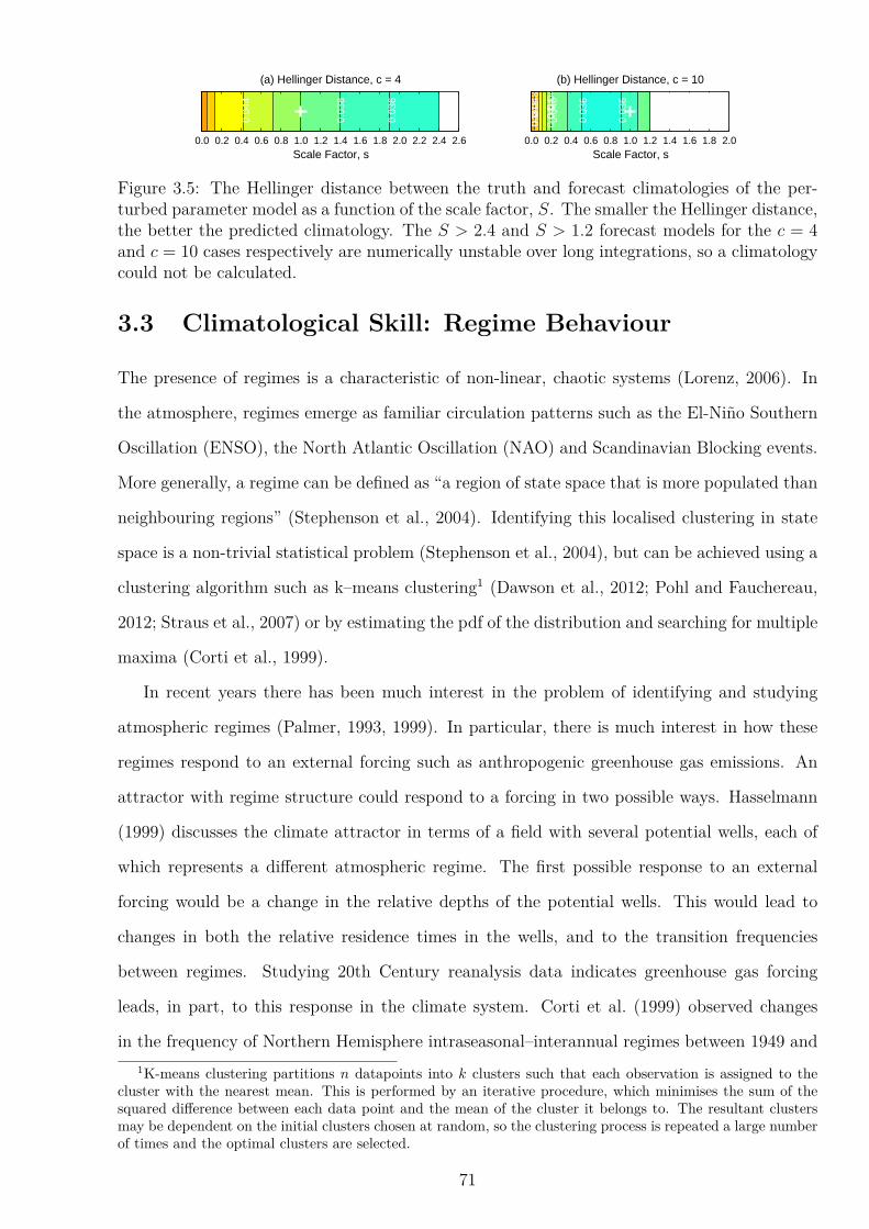
0.04
0.04
0.040.
048
0.04
80.
048
Scale Factor, s
(b) Hellinger Distance, c = 10
0.03
6
0.03
6
0.04
0
0.0 0.2 0.4 0.6 0.8 1.0 1.2 1.4 1.6 1.8 2.0Scale Factor, s
(a) Hellinger Distance, c = 4
0.03
6
0.03
8
0.04
4
0.0 0.2 0.4 0.6 0.8 1.0 1.2 1.4 1.6 1.8 2.0 2.2 2.4 2.6
Figure 3.5: The Hellinger distance between the truth and forecast climatologies of the per-turbed parameter model as a function of the scale factor, S. The smaller the Hellinger distance,the better the predicted climatology. The S > 2.4 and S > 1.2 forecast models for the c = 4and c = 10 cases respectively are numerically unstable over long integrations, so a climatologycould not be calculated.
3.3 Climatological Skill: Regime Behaviour
The presence of regimes is a characteristic of non-linear, chaotic systems (Lorenz, 2006). In
the atmosphere, regimes emerge as familiar circulation patterns such as the El-Nino Southern
Oscillation (ENSO), the North Atlantic Oscillation (NAO) and Scandinavian Blocking events.
More generally, a regime can be defined as “a region of state space that is more populated than
neighbouring regions” (Stephenson et al., 2004). Identifying this localised clustering in state
space is a non-trivial statistical problem (Stephenson et al., 2004), but can be achieved using a
clustering algorithm such as k–means clustering1 (Dawson et al., 2012; Pohl and Fauchereau,
2012; Straus et al., 2007) or by estimating the pdf of the distribution and searching for multiple
maxima (Corti et al., 1999).
In recent years there has been much interest in the problem of identifying and studying
atmospheric regimes (Palmer, 1993, 1999). In particular, there is much interest in how these
regimes respond to an external forcing such as anthropogenic greenhouse gas emissions. An
attractor with regime structure could respond to a forcing in two possible ways. Hasselmann
(1999) discusses the climate attractor in terms of a field with several potential wells, each of
which represents a different atmospheric regime. The first possible response to an external
forcing would be a change in the relative depths of the potential wells. This would lead to
changes in both the relative residence times in the wells, and to the transition frequencies
between regimes. Studying 20th Century reanalysis data indicates greenhouse gas forcing
leads, in part, to this response in the climate system. Corti et al. (1999) observed changes
in the frequency of Northern Hemisphere intraseasonal–interannual regimes between 1949 and
1K-means clustering partitions n datapoints into k clusters such that each observation is assigned to thecluster with the nearest mean. This is performed by an iterative procedure, which minimises the sum of thesquared difference between each data point and the mean of the cluster it belongs to. The resultant clustersmay be dependent on the initial clusters chosen at random, so the clustering process is repeated a large numberof times and the optimal clusters are selected.
71

1994, though the structure of the regimes remained unchanged over this time period.
The second possible response to an external forcing is a change in regime properties, such
as centroid location and number of regimes (i.e. the position and number of potential wells). In
addition to observing changes in frequency of regimes over the time period 1948–2002, Straus
et al. (2007) observe this second type of response in the reanalysis data; the structure of the
Pacific trough regime is statistically significantly different at the end of the time period than
at the beginning.
The importance of regimes in observed trends over the past 50–100 years indicates that in
order to predict anthropogenic climate change, our climate models must be able to accurately
represent natural circulation regimes, their statistics and variability. Dawson et al. (2012) show
that while NWP models are able to capture the regime behaviour of the climate system with
reasonable accuracy, the same model run at climate resolution does not show any statistically
significant regime structure. However, the model used in this study has no representation of
model uncertainty; a single deterministic forecast is made from each starting date.
It is now well established that representing model uncertainty as well as initial condition
uncertainty is important for reliable weather forecasts (Ehrendorfer, 1997). Many possible
methods for representing model uncertainty have been discussed in Section 1.3. It is possible
that including a representation of model uncertainty could enable the simulator to explore
larger regions of the climate attractor, including other flow regimes. This section seeks to
investigate the effect of including representations of model uncertainty on the regime beha-
viour of a simulator. A deterministic parametrisation scheme will be compared to stochastic
parametrisation approaches and a perturbed parameter ensemble (please refer to Chapter 2
for experimental details). A simple chaotic model of the atmosphere, the L96 system, will be
used to study the predictability of regime changes (Lorenz, 1996, 2006).
3.3.1 Data and Methods
The Lorenz (1996) simplified model of the atmosphere was used in this investigation, as de-
scribed in Chapter 2. Firstly, it needs to be established whether the L96 two–scale model ex-
hibits regime behaviour. Lorenz (2006) carried out a series of experiments using the one-scale
Lorenz ’96 system (hereafter L96 1D), which describes the evolution of the L96 Xk variables,
72

Figure 3.6: The time series of total energy for the L96 1D system, where total energy is definedas E = 1
2
∑X2
k . The labels [4.95–5.25] indicate the value of the forcing, F , in (3.4). Takenfrom Lorenz (2006) (Fig. 3).
73

0 20 40 60 80 100 120 140 160 180 200
100
200
300
Time / MTU.T
otal
Ene
rgy
Figure 3.7: The time series of total energy for the L96 system, c = 4 case, where total energy isdefined as E = 1
2
∑X2
k . Total energy is not conserved as the system is forced and dissipative.The time series for total energy does not appear to show regime behaviour for the c = 4 casewith forcing F = 20.
without the influence of the smaller scale Yj variables (Lorenz, 1996):
dXk
dt= −Xk−1(Xk−2 −Xk+1) −Xk + F k = 1, ..., K (3.4)
Lorenz defines a dynamical system as having regime behaviour if:
1. The phase space of the dynamical system has two separate regions, A and B.
2. Both transitions A–B and B–A are observed.
3. For both modes, the average length of time between transitions must be long compared
to some other significant oscillation of the system.
He performed extended numerical runs and examined the resultant time series of total energy.
E =1
2
K∑
k=1
X2k (3.5)
Figure 3.6 shows the time series for the L96 1D system for different values of the forcing
parameter, F . From his criteria, Lorenz identified regimes in the time series for F = 5.05−5.25.
Figure 3.7 and Figure 3.8(a) show the time series of total energy for the c = 4 and c = 10
cases for the L96 system respectively. The c = 4 case does not appear to have regimes as
defined by Lorenz (2006) for F = 20. However, the c = 10 case shows drops in the total energy
of the system which persist for a few model time units, which could indicate the presence of
regimes. The time series for c = 10 looks qualitatively similar to the series for F = 5.25 in
Figure 3.6, for the L96 1D system.
Lorenz also considers the spatial distribution of the X variables as a test for the presence of
regimes. Figure 3.9 (a) shows profiles of the L96 system Xk at 6 hour intervals taken from 60
MTU after the start of the dataset in Figure 3.8, when the total energy of the system tends to
74

0 20 40 60 80 100 120 140 160 180 200
100
150
200
Time / MTU.
Tot
al E
nerg
y
(a)
0 20 40 60 80 100 120 140 160 180 200−20
−10
0
10
20
Cov
aria
nce
diag
nost
ic
Time / MTU.
(b)
0 20 40 60 80 100 120 140 160 180 200
B
A
Reg
ime
Time / MTU.
(c)
Figure 3.8: (a) The time series of total energy for the L96, c = 10, F = 20 case, where totalenergy is defined as E = 1
2
∑X2
k . (b) The covariance diagnostic evaluated for the data shown in(a). If the diagnostic is positive, a wave–2 pattern dominates the behaviour of the X variables,whereas if it is negative, a wave–1 pattern is dominant. See text for details. (c) The same dataset, interpreted in terms of two regimes — A and B — defined using the covariance diagnostic.If the diagnostic is positive, the system is interpreted as being in Regime A.
be higher with large oscillations. Figure 3.9 (b) shows profiles from 50 MTU after the start of
the dataset, when the total energy of the system has dropped to a lower, more quiescent state.
The two sets of profiles are different: since these two samples are characterised by physically
different states, it is reasonable to interpret them as coming from two different regimes.
The difference in structure between the two regimes is most clearly revealed by consideration
of the covariance matrix of the X variables, shown in Figure 3.10. It is convenient to define
Regimes A and B in terms of this covariance matrix C, calculated using samples of the time
series 1 MTU long, where C(m,n) represents the covariance between Xm and Xn:
Regime = A ⇐⇒ (C(1, 5) + C(2, 6) + C(3, 7) + C(4, 8)) > 0
Regime = B ⇐⇒ (C(1, 5) + C(2, 6) + C(3, 7) + C(4, 8)) < 0 (3.6)
In other words, the system is defined to be in Regime A if opposite X variables are in phase
for K = 8, and in Regime B if opposite X variables are out of phase. The time series of this
“covariance diagnostic” and the resultant identified regimes are shown in Figure 3.8 (b) and
75

1 2 3 4 5 6 7 8X
k
0
1
2
(b)
1 2 3 4 5 6 7 8X
k
0
1
2
(a)
Figure 3.9: Profiles of the K = 8 X variables for the L96 c = 10 case. The profiles are takenfrom (a) 60 MTU and (b) 50 MTU after the start of the time series shown in Figure 3.8. Thelabelling on the Y-axis indicates the number of “atmospheric days” since the first profile. Theprofiles from Regime A show a wave–2 type behaviour, while those from Regime B show adominant wave–1 pattern.
−10
−10 −10
0
0
0
0
0
0
10
10
100
0
0
0
0
0
−10
−10
−10−10 20
20
−10 −10
10
0
0 10
30
0
0
Xm
Xn
(a)
1 2 3 4 5 6 7 81
2
3
4
5
6
7
8
−10
−10
−10
−10
0
0 0
0
0
10
10
10
10
10
10
−10
−1020
20
0
0
−20
−2030
Xm
Xn
(b)
1 2 3 4 5 6 7 81
2
3
4
5
6
7
8
Figure 3.10: The covariance matrix, C(m,n), for the covariance between Xm and Xn calculatedfrom a 1 MTU sample, (a) 60 MTU and (b) 50 MTU after the start of the time series shownin Figure 3.8. (a) The dominant feature is a wave–2 pattern, with the ‘opposite’ X variablesin phase with each other. (b) The dominant feature is a wave–1 pattern, with the ‘opposite’X variables out of phase with each other.
0 10 20 30 400
0.02
0.04
0.06
0.08
0.1
(a)
Duration / MTU
Fre
quen
cy D
ensi
ty
0 2 4 6 8 100
0.05
0.1
0.15
0.2
0.25
0.3
0.35
0.4
0.45(b)
Duration / MTU
Fre
quen
cy D
ensi
ty
Figure 3.11: The probability distribution function (pdf) for the duration of (a) Regime A and(b) Regime B. Regime A events are observed to be longer lasting on average than Regime Bevents.
76

1 2 3 4 5 6 7 8
−0.5
0
0.5
X
Mag
nitu
de
EOF 1 EOF 2 EOF 3 EOF 4
Figure 3.12: The first four Empirical Orthogonal Functions (EOFs) calculated from the c = 10truth time series. Due to the symmetry of the system, the EOFs correspond to the leadingharmonics.
(c) respectively.
Lorenz’s third criterion for regimes requires their duration to be longer than some other
significant oscillation of the system. In the L96 system for the c = 10 case, the dominant
oscillation of the X variables has a time period of approximately 0.5 MTU. Figure 3.11 shows
a pdf of the duration of each regime. The average duration of Regime A is 5.08 MTU, and the
average duration of Regime B is 2.06 MTU. The average duration of both regimes is greater
than 0.5 MTU, so we can conclude that, for the c = 10 case, the L96 system does indeed
exhibit regime behaviour, and is a suitable model for use in this investigation.
The predictability of the regime behaviour of the L96 system, c = 10 case, will be studied
using the same techniques used for atmospheric data. Firstly, it has been suggested that the
time series should be temporally smoothed to help identify the regimes (Straus et al., 2007;
Stephenson et al., 2004). For example, consider the well–known Lorenz (1963) system (the
“butterfly attractor”): the system clearly has two regimes corresponding to the two lobes of
the attractor, but these regimes are only apparent in a pdf of the system if the time series is
first temporally averaged (Corti et al., 1999; Stephenson et al., 2004)2. In the L96 system, the
modal residence time in Regime B is ∼ 0.4 MTU (Figure 3.11), so a running time average over
0.4 MTU will be used to smooth the time series.
When studying atmospheric data sets, the dimensionality of the problem is usually reduced
using an empirical orthogonal function (EOF) analysis on the temporally smoothed data series
2The time series must not be too heavily smoothed as this will cause the pdf to tend towards a Gaussiandistribution (following the central limit theorem).
77

(Straus et al., 2007). Due to the symmetry of the L96 system, Figure 3.12 shows that the leading
EOFs of the L96 system are simply the dominant harmonics. The first two EOFs are degenerate,
and are π4
out of phase wavenumber two oscillations, i.e. are in phase quadrature. The third
and fourth EOFs are similarly in phase quadrature, and are π2
out of phase wavenumber one
oscillations. Consideration of Figure 3.12 shows that EOF1 and EOF2 are likely to dominate
in Regime A, whereas EOF3 and EOF4 dominate in Regime B. The principal components
(PCs) were calculated for each EOF. Due to the degeneracies of the EOFs, the magnitude of
the principal component vectors, ||[PC1, PC2]|| and ||[PC3, PC4]||, will be considered and the
pdf of the system plotted in this space.3 The corresponding eigenvalues show that EOF1 and
EOF2 account for 68.7% of the variance, while EOF3 and EOF4 account for a further 14.4%.
3.3.2 The True Attractor
The full set of c = 10 L96 equations is integrated forward for 10,000 MTU ∼ 140 “atmospheric
years” to ensure the attractor is fully sampled. The time series is temporally smoothed with
a running average over 0.4 MTU. For comparison, the raw, unsmoothed time series is also
considered. An EOF decomposition is carried out on each of the truth time series (raw and
smoothed), and the PCs calculated. The dimensionality of the space is further reduced by
considering only the magnitude of the PC vectors [PC1, PC2] and [PC3, PC4] as a function
of time. The state vector pdf for the full “truth” model is shown in Figure 3.13 for (a)
the unsmoothed time series and (b) the smoothed time series. Temporally smoothing the
time series helps to identify the two regimes. The maximum of the pdf is located at large
[PC1, PC2] and small [PC3, PC4], corresponding to the more common wave–2 “Regime A”
state of the system. However, in (b) the pdf is elongated away from this maximum towards
large [PC3, PC4] and small [PC1, PC2], where there is a small but distinct subsidiary peak;
this corresponds to the less common “Regime B”. Figure 3.13(a) does not have a distinct second
peak, so does not indicate the presence of regimes.
Figures 3.13(c) and (d) show the mean residence time of trajectories within local areas of
phase space. For each point in PC space, a circular region with radius R is defined, and the
3This is equivalent to considering complex EOFs, which are used to capture propagating modes. A Hilberttransform is applied to the time series X to calculate H(X), which includes information about the first derivativeof the data, and indicates the presence of the orthogonal sine/cosine signals necessary for a propagating signal.A standard EOF analysis is then performed for the modified time series: X + H(X). In this study, EOF1 andEOF2 together represent the first complex EOF, and EOF3 and EOF4 represent the second complex EOF.
78

average residence time of trajectories within that region is calculated, following Frame et al.
(2013). Here R = 2, and the displayed circle indicates the size of the region for comparison. For
both (c) the unsmoothed and (d) the smoothed time series, two regions of high residence time
can be identified. The longest residence times occur at large [PC1, PC2] and small [PC3, PC4],
corresponding to Regime A. There is a further peak in residence time at large [PC3, PC4]
and small [PC1, PC2], corresponding to Regime B. These two distinct peaks provide further
evidence for the regime nature of the L96 system: there are two regions in phase space which
the system preferentially occupies for extended periods of time, and transitions between these
regions are more rapid. This diagnostic confirms that Regime A is more persistent than Regime
B, as expected from Figure 3.11.
Figures 3.13(e) and (f) show the mean velocity of the system’s motion through phase space.
The colour indicates mean speed, and arrows indicate mean direction. A region with radius 0.5
is defined centred on each point in phase space, and the net displacement of trajectories starting
within this region is calculated over 0.05 MTU. The average magnitude and average direction
of displacement is then calculated. Both Figures (e) and (f) show two centres of rotation in
phase space corresponding to the two regimes. On average, trajectories circle these centres,
resulting in persistent conditions (cf. the Lorenz ’63 ‘butterfly attractor’). The structure of
the flow field is somewhat different for the smoothed time series — the second centre is less
clearly defined, but coincides with a maximum in the average magnitude of displacement.
In fact, trajectories are observed to oscillate vertically about this centre during a persistent
Regime B phase, resulting in the large average magnitude, but small average displacement
vector. Nevertheless, both Figures 3.13(e) and (f) provide conclusive evidence of the existence
of regimes in the L96 system, which can be detected in both the raw and smoothed data.
3.3.3 Simulating the Attractor
Having demonstrated that the full L96 system exhibits regime behaviour, the skill of each of
the truncated L96 forecast models at reproducing this regime behaviour will be evaluated.
Each forecast model is integrated forward for 10,000 MTU as for the full L96 system. For
the perturbed parameter experiment, each of the 40 deterministic models is integrated for
250 MTU. While regime behaviour can be detected in both the raw and smoothed truth time
series, the results in Section 3.3.2 indicate that it is easier to detect the presence of regimes in
79

(a)
|| [PC 1, PC 2] ||
|| [P
C 3
, PC
4] |
|
0 5 10 150
5
10
15
0
0.005
0.01
0.015
0.02
0.025
0.03(b)
|| [PC 1, PC 2] ||
|| [P
C 3
, PC
4] |
|
0 5 100
2
4
6
8
10
12
0
0.02
0.04
0.06
0.08
(c)
|| [PC 1, PC 2] ||
|| [P
C 3
, PC
4] |
|
0 5 10 150
5
10
15
0
0.05
0.1
(d)
|| [PC 1, PC 2] ||
|| [P
C 3
, PC
4] |
|
0 5 100
2
4
6
8
10
12
0.05
0.1
0.15
0.2
0.25
0.3
0.35
0.4
(e)
|| [PC 1, PC 2] ||
|| [P
C 3
, PC
4] |
|
0 5 10 150
5
10
15
0
1
2
3
4(f)
|| [PC 1, PC 2] ||
|| [P
C 3
, PC
4] |
|
0 5 100
2
4
6
8
10
12
0
0.5
1
1.5
2
Figure 3.13: Regime characteristics of the full L96 system. Both the raw and temporallysmoothed time series are considered, where the smoothing is a running average over 0.4MTU. Each diagnostic is shown in the space of pairs of leading EOFs, [EOF1, EOF2] and[EOF3, EOF4]. See text for details. (a) Raw and (b) smoothed pdfs. (c) Raw and (d)smoothed mean residence times (MTU): the mean length of time a trajectory remains within 2units of each location. A circle of radius two is indicated. (e) Raw and (f) smoothed magnitude(colour) and orientation (arrows) of the average displacement in phase space over 0.05MTU ,averaged over trajectories passing within 0.5 units of each position in phase space.
80
the smoothed time series pdf, as was suggested by Straus et al. (2007). Therefore, the time
series are temporally smoothed with a running average over 0.4 MTU. The four leading order
truth EOFs are used to calculate the PCs of the forecast models to ensure a fair comparison
(Corti et al., 1999). The dimensionality of the space is further reduced by considering only the
magnitude of the PC vectors [PC1, PC2] and [PC3, PC4] as a function of time (equivalent
to considering the first two complex EOFs). The state vector pdfs for each of the forecast
models considered are shown in Figure 3.14; the pdf for the full “truth” model has also been
reproduced for ease of comparison.
Panel (a) in Figure 3.14 corresponds to the full “truth” equations (1.6), reproduced from
Figure 3.13, and shows two distinct peaks corresponding to the two regimes, A and B. None of
the forecast models are able to accurately capture the second subsidiary peak, corresponding
to Regime B. The white noise stochastic models and the deterministic (DET) parametrisation
scheme all put too little weight on this area of phase space. However, the AR(1) stochastic
models show a large improvement — Regime B is explored more frequently than by the determ-
inistic or white stochastic models, though not as frequently as by the full truth system. The
attractor of the perturbed parameter model, Figure 3.14(c), shows a distinct peak for Regime
B, unlike the other forecast models. However, the attractor has a very different structure to
that for the truth time series — Regime B is visited too frequently.
In fact, it is surprising how reasonable the perturbed parameter attractor looks! It consists
of an average of 40 constituent members, shown in Figure 3.15. The contour colours are
consistent with Figure 3.14. Many of the 40 different perturbed parameter ensemble members
show vastly different regime behaviour to the true attractor. While some ensemble members (for
example, numbers 8, 13, 18 and 38) look reasonable, many spend all their time in Regime A
and do not explore Regime B at all (for example, numbers 1–4, etc), while some predominantly
inhabit Regime B (e.g. numbers 5, 37, 39). Perturbed parameter ensembles are often used for
climate prediction. However, if individual members only explore one region of the true climate
attractor, how can the effect of forcing on the frequency of different regimes be established?
For ease of comparison, the 2D Figure 3.14 has been decomposed into two, 1D pdfs for
each of the forecast models (Figure 3.16). The Kolmogorov-Smirnov Statistic (3.1), Dks, and
Hellinger distance (3.2), DHell, have been calculated as measures of the difference between the
true pdf and the forecast pdf for each case. For both Dks and DHell, the smaller the measure,
81

(a) TRU
|| [PC 1, PC 2] ||
|| [P
C 3
, PC
4] |
|
0 5 10 150
2
4
6
8
10
0
0.02
0.04
0.06
0.08
(b) DET
|| [PC 1, PC 2] ||
|| [P
C 3
, PC
4] |
|
0 5 10 150
2
4
6
8
10(c) PP
|| [PC 1, PC 2] ||
|| [P
C 3
, PC
4] |
|
0 5 10 150
2
4
6
8
10
(d) WA
|| [PC 1, PC 2] ||
|| [P
C 3
, PC
4] |
|
0 5 10 150
2
4
6
8
10(e) AR1A
|| [PC 1, PC 2] ||
|| [P
C 3
, PC
4] |
|
0 5 10 150
2
4
6
8
10
(f) WM
|| [PC 1, PC 2] ||
|| [P
C 3
, PC
4] |
|
0 5 10 150
2
4
6
8
10(g) AR1M
|| [PC 1, PC 2] ||
|| [P
C 3
, PC
4] |
|
0 5 10 150
2
4
6
8
10
Figure 3.14: Ability of different parametrisation models to reproduce the true attractor (topleft). The pdf of the state vector for the c = 10 L96 system is plotted in the space of pairs ofleading EOFs. See text for details. Six different forecasting models are shown. (b) Determ-inistic parametrisation scheme; (c) perturbed parameter scheme; additive stochastic paramet-risation with (d) white and (e) AR(1) noise; multiplicative stochastic parametrisation with (f)white and (g) AR(1) noise. The degree of perturbation of the perturbed parameters, and thestandard deviation and autocorrelation in the stochastic parametrisations have been estimatedfrom the truth time series (see Chapter 2 for more details). The same EOFs determined fromthe full truth data set are used in each panel, and the colour of the contours is also consistent.
82
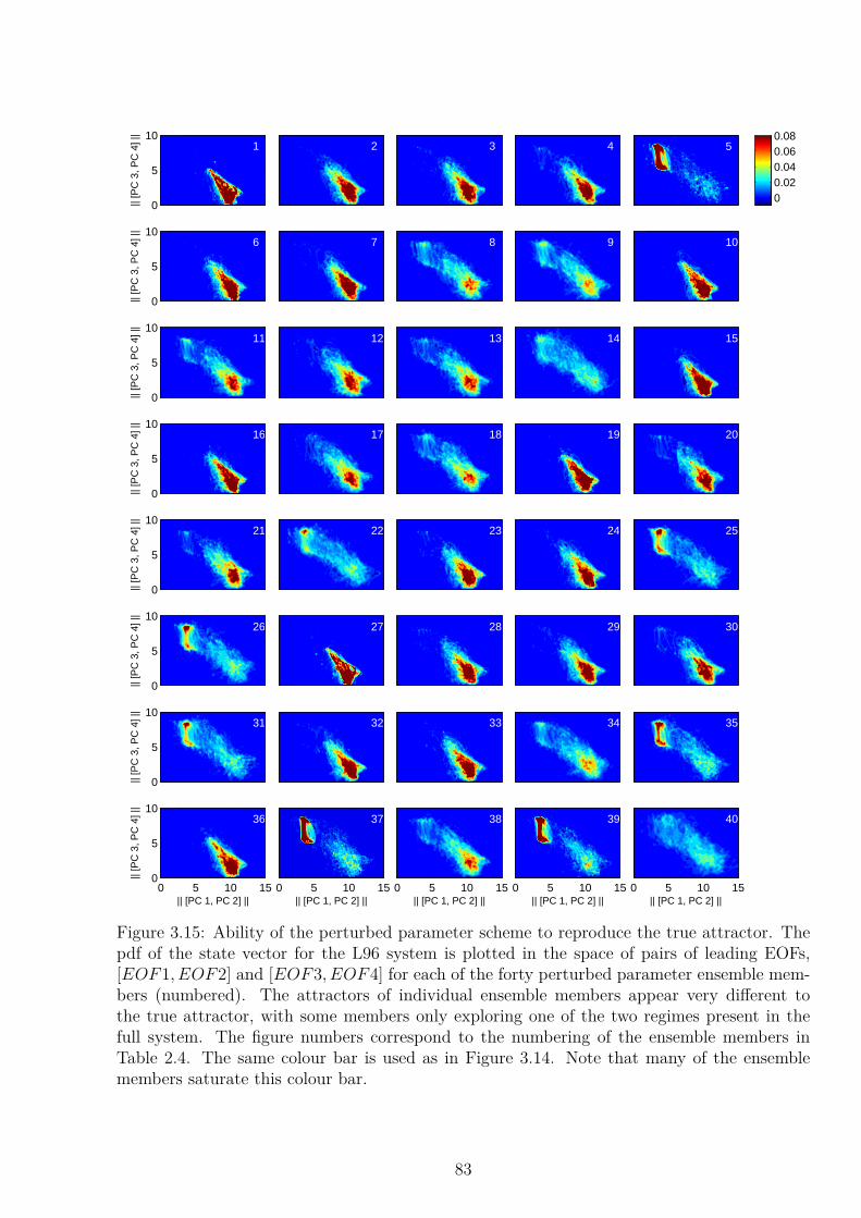
|| [P
C 3
, PC
4] |
|1
0
5
102 3 4
5
00.020.040.060.08
|| [P
C 3
, PC
4] |
|
6
0
5
107 8 9 10
|| [P
C 3
, PC
4] |
|
11
0
5
1012 13 14 15
|| [P
C 3
, PC
4] |
|
16
0
5
1017 18 19 20
|| [P
C 3
, PC
4] |
|
21
0
5
1022 23 24 25
|| [P
C 3
, PC
4] |
|
26
0
5
1027 28 29 30
|| [P
C 3
, PC
4] |
|
31
0
5
1032 33 34 35
|| [PC 1, PC 2] ||
|| [P
C 3
, PC
4] |
|
36
0 5 10 150
5
10
|| [PC 1, PC 2] ||
37
0 5 10 15|| [PC 1, PC 2] ||
38
0 5 10 15|| [PC 1, PC 2] ||
39
0 5 10 15|| [PC 1, PC 2] ||
40
0 5 10 15
Figure 3.15: Ability of the perturbed parameter scheme to reproduce the true attractor. Thepdf of the state vector for the L96 system is plotted in the space of pairs of leading EOFs,[EOF1, EOF2] and [EOF3, EOF4] for each of the forty perturbed parameter ensemble mem-bers (numbered). The attractors of individual ensemble members appear very different tothe true attractor, with some members only exploring one of the two regimes present in thefull system. The figure numbers correspond to the numbering of the ensemble members inTable 2.4. The same colour bar is used as in Figure 3.14. Note that many of the ensemblemembers saturate this colour bar.
83

0 5 10 150
0.05
0.1
0.15
0.2
0.25
0.3
|| [PC1, PC2] ||
Pro
babi
lity
Den
sity
(a)
0 2 4 6 8 100
0.05
0.1
0.15
0.2
0.25
0.3
|| [PC3, PC4] ||
Pro
babi
lity
Den
sity
(b)
TRU DET AR1 A AR1 M PP
Figure 3.16: Ability of different parametrisation models to reproduce two of the dimensions ofthe true attractor, shown as two 1–dimensional plots. The pdf of the state vector for the L96system is plotted for (a) the magnitude of [PC1, PC2] and (b) the magnitude of [PC3, PC4].Four different forecasting models are shown on each panel (coloured lines) together with thatfor the truth data. White noise, whether additive or multiplicative, is indistinguishable fromthe deterministic case, so has not been shown.
Parametrisation[PC1,PC2] [PC3,PC4]Dks Dhell Dks Dhell
Deterministic 0.083 0.125 0.112 0.117White Additive Stochastic 0.084 0.125 0.114 0.118AR(1) Additive Stochastic 0.037 0.062 0.049 0.055White Multiplicative Stochastic 0.083 0.121 0.110 0.115AR(1) Multiplicative Stochastic 0.040 0.052 0.028 0.035Perturbed Parameters 0.072 0.110 0.040 0.048
Table 3.1: The skill of different parametrisation schemes at reproducing the structure of theTruth attractor along each of two directions defined by the dominant EOFs. The Kolmogorov-Smirnov distance Dks, and Hellinger distance Dhell, are used to measure the similarity betweenthe true and forecast pdfs. The smaller each of these measures, the closer the forecast pdf isto the true pdf. The best forecast model according to each measure is shown in red.
84

the closer the forecast is to the true pdf. The results are shown in Table 3.1. The AR(1)
multiplicative stochastic forecast is the most skilful for each case according to the Hellinger
distance. The AR(1) additive scheme also scores well for both cases, and is the most skilful
representation of [PC1, PC2] according to the Kolmogorov-Smirnov distance. The perturbed
parameter ensemble greatly improves over the deterministic and white stochastic forecasts
for the [PC3, PC4] case, but does not greatly improve over the deterministic scheme for the
[PC1, PC2] pdf.
However, a perturbed parameter ensemble must be interpreted carefully. Since each member
of the ensemble is a physically distinct model of the system, the forecast climatology of each
member should be assessed individually. The 1D pdfs of [PC1, PC2] and [PC3, PC4] were
calculated for each ensemble member, and the Hellinger distance between the forecast and true
pdfs evaluated for each case. For comparison, the deterministic and stochastic forecasts were
also split into 40 sections, each 250 MTU long, and the Hellinger distance evaluated for each
section as for the perturbed parameter ensemble. This allows the effect of sampling error to be
considered. The distribution of Hellinger distances for each case is shown in Figure 3.17. The
spread of skill is largest for the perturbed parameter ensemble, with some members showing
very poor climatologies, while others are more skilful. The white additive and multiplicative
schemes do not show a significant difference from the deterministic forecast, while the AR1
additive and AR1 multiplicative schemes are consistently better than the other schemes.
3.3.4 Simulating Regime Statistics
While reproducing the pdf of the true system is important for capturing regime behaviour, it is
also necessary for a forecast model to represent the temporal characteristics of the regimes well.
This is evaluated using the distribution of persistence of each regime (Dawson et al., 2012; Pohl
and Fauchereau, 2012; Frame et al., 2013), and will be considered using two different techniques.
Firstly, the behaviour of the system in PC space is used to examine the temporal character-
istics of the system. The mean residence time of trajectories in phase space is calculated. For
each point in PC space, a circular region with radius R is defined, and the average residence
time of trajectories within that region is calculated, as for Figure 3.13(c) and (d). Figure 3.18
shows the mean residence time of trajectories when R = 2 PC units, and Figure 3.19 shows the
same diagnostic when R = 4 PC units. For each case, the circle in panel (a) indicates the size
85

DET WA AR1A WM AR1M PP0
0.1
0.2
0.3
0.4
0.5
Forecast Scheme
[PC1, PC2](a)
Dis
trib
utio
n of
Hel
linge
r D
ista
nces
DET WA AR1A WM AR1M PP0
0.1
0.2
0.3
0.4
Forecast Scheme
[PC3, PC4](b)
Dis
trib
utio
n of
Hel
linge
r D
ista
nces
Figure 3.17: The distribution of Hellinger distance calculated for the difference between fore-cast and observed EOF climatologies. The pdf for the magnitude of (a) [PC1, PC2] and (b)[PC3, PC4] is calculated. For the deterministic and stochastic models, the time series is splitinto 40 sections, 250 MTU long, and the pdfs calculated for each. For the perturbed parameterensemble, the pdfs are calculated for each ensemble member separately. The Hellinger distancebetween each forecast pdf and the true pdf is evaluated, and the distribution of Hellinger dis-tance represented by a box and whisker plot. The median value is marked by a horizontal redline. The 25th and 75th percentiles are indicated by the edges of the box, and the whiskersextend to the minimum and maximum value in each case, unless there are outliers, which aremarked by a red cross. An outlier is defined as a value smaller than 1.5 times the inter–quartilerange (IQR) below the lower quartile, or greater than 1.5 IQR above the upper quartile.
of the region. For both R = 2 and R = 4, two regions of comparatively high residence time
can be identified in the truth simulation shown in panel (a). The longest residence times occur
at large [PC1, PC2] and small [PC3, PC4], corresponding to Regime A. There is a smaller
peak in residence time at large [PC3, PC4] and small [PC1, PC2], corresponding to Regime
B. Figures 3.18 (a) and 3.19 (a) are qualitatively similar, except that the peaks have a more
equal depth for the R = 2 case than for the R = 4 case.
The forecast models are able to capture the temporal characteristics of the true system. They
show two distinct peaks in residence time of approximately the correct magnitude. However,
there are subtle differences between the different forecast models. In Figure 3.18, the DET, PP,
WA and WM forecast models have regimes that are too persistent — the two peaks in residence
time are too high, particularly for Regime A. The red noise stochastic schemes perform better,
with the AR1M scheme capturing the average residence time for Regime B particularly well.
In Figure 3.19, all models predict too high residence times for Regime A. However, the AR1M
scheme performs the best, with a good representation of residence times in the tail of the pdf,
and a lower and more accurate peak residence time for Regime A.
86

(a) TRU
|| [PC 1, PC 2] ||
|| [P
C 3
, PC
4] |
|
0 5 10 150
2
4
6
8
10
0
0.1
0.2
0.3
0.4
0.5
(b) DET
|| [PC 1, PC 2] ||
|| [P
C 3
, PC
4] |
|
0 5 10 150
2
4
6
8
10
(c) PP
|| [PC 1, PC 2] ||
|| [P
C 3
, PC
4] |
|
0 5 10 150
2
4
6
8
10
(d) WA
|| [PC 1, PC 2] ||
|| [P
C 3
, PC
4] |
|
0 5 10 150
2
4
6
8
10
(e) AR1A
|| [PC 1, PC 2] ||
|| [P
C 3
, PC
4] |
|
0 5 10 150
2
4
6
8
10
(f) WM
|| [PC 1, PC 2] ||
|| [P
C 3
, PC
4] |
|
0 5 10 150
2
4
6
8
10
(g) AR1M
|| [PC 1, PC 2] ||
|| [P
C 3
, PC
4] |
|
0 5 10 150
2
4
6
8
10
Figure 3.18: Mean residence time in model time units. The mean length of time trajectoriesremain within 2 units of each position in PC space. A circle of radius 2 units is shown forcomparison in panel (a).
87

(a) TRU
|| [PC 1, PC 2] ||
|| [P
C 3
, PC
4] |
|
0 5 10 150
2
4
6
8
10
0
1
2
3
4
5
(b) DET
|| [PC 1, PC 2] ||
|| [P
C 3
, PC
4] |
|
0 5 10 150
2
4
6
8
10
(c) PP
|| [PC 1, PC 2] ||
|| [P
C 3
, PC
4] |
|
0 5 10 150
2
4
6
8
10
(d) WA
|| [PC 1, PC 2] ||
|| [P
C 3
, PC
4] |
|
0 5 10 150
2
4
6
8
10
(e) AR1A
|| [PC 1, PC 2] ||
|| [P
C 3
, PC
4] |
|
0 5 10 150
2
4
6
8
10
(f) WM
|| [PC 1, PC 2] ||
|| [P
C 3
, PC
4] |
|
0 5 10 150
2
4
6
8
10
(g) AR1M
|| [PC 1, PC 2] ||
|| [P
C 3
, PC
4] |
|
0 5 10 150
2
4
6
8
10
Figure 3.19: Mean residence time in model time units. The mean length of time trajectoriesremain within 4 units of each position in PC space. A circle of radius 4 units is shown forcomparison in panel (a).
88

As for the pdf of the state vector, it is important to recall that the PP ensemble consists
of 40 physically distinct representations of the system. The residence time pdfs are plotted for
each perturbed parameter ensemble member in Figure 3.20 for the R = 2 case. The individual
ensemble members have vastly different temporal characteristics. Some members show very
persistent regimes with very few transitions, and some (e.g. 8, 13) indicate the presence of a
third regime. The same colour scale is used as for Figure 3.18, but has saturated for several
panels. For example, the maximum residence time of Regime A for ensemble member 1 is 1.08
MTU, which is more than double the maximum residence time observed in the full system.
Similarly, the maximum residence time of Regime B for ensemble member 5 is 2.04 MTU,
more than six times greater than that observed for Regime B in the full system. Considered
individually, the PP ensemble members are a poor representation of the regime behaviour of
the true system.
The second technique used to study the regime statistics uses the definition of Regimes
A and B given by (3.6). The definition is used to determine the regime at each time step,
and the pdf of persistence of each regime calculated as for Figure 3.11. Figure 3.21 compares
the persistence pdfs for the full L96 system with that of the truncated forecast models. The
AR(1) stochastic parametrisation schemes (red and magenta lines) improve significantly over
the white stochastic schemes (blue and cyan) and the deterministic scheme (green) — the
distribution of regime durations more closely matches the true distribution for the AR(1) noise
cases. The proportion of time spent in each regime also improves (Table 3.2); the deterministic
and white noise schemes visit Regime B too rarely, whereas the proportion of time spent in
Regime B by the AR(1) stochastic schemes is close to the truth.
The perturbed parameter scheme (grey lines) appears to perform very well. Table 3.2
shows that averaged over all ensemble members, the proportion of time spent in each regime
very accurately represents the true system. Figure 3.21 shows that the frequency and duration
of the modal persistence match the truth time series well for both Regime A and Regime B.
However, this figure is misleading. The tail of the perturbed parameter pdf extends well beyond
the X–axis limit for both Figures (a) and (b), as some ensemble members showed very persistent
regimes with only rare transitions, as indicated in Figure 3.20. The members with only one or
two transitions only contribute one or two persistence values to the data set, so affect the modal
height and position very little. Nevertheless, it is interesting to see how, while each individual
89

|| [P
C 3
, PC
4] |
|
1
0
5
10 2 3 4
5
0
0.2
0.4
|| [P
C 3
, PC
4] |
|
6
0
5
10 7 8 9 10
|| [P
C 3
, PC
4] |
|
11
0
5
10 12 13 14 15
|| [P
C 3
, PC
4] |
|
16
0
5
10 17 18 19 20
|| [P
C 3
, PC
4] |
|
21
0
5
10 22 23 24 25
|| [P
C 3
, PC
4] |
|
26
0
5
10 27 28 29 30
|| [P
C 3
, PC
4] |
|
31
0
5
10 32 33 34 35
|| [PC 1, PC 2] ||
|| [P
C 3
, PC
4] |
|
36
0 100
5
10
|| [PC 1, PC 2] ||
37
0 10|| [PC 1, PC 2] ||
38
0 10|| [PC 1, PC 2] ||
39
0 10|| [PC 1, PC 2] ||
40
0 10
Figure 3.20: Mean residence time in model time units for each member of the perturbedparameter ensemble. The mean length of time trajectories remain within 2 units of eachposition in PC space. The figure numbers correspond to the numbering of the ensemblemembers in Table 2.4.
90

0 10 20 30 400
0.02
0.04
0.06
0.08
0.1
(a)
Duration / MTU
Fre
quen
cy D
ensi
ty
Regime A
TRU DET W A AR1 A W M AR1 M PP
0 2 4 6 8 100
0.1
0.2
0.3
0.4
0.5
(b)
Duration / MTU
Fre
quen
cy D
ensi
ty
Regime B
Figure 3.21: Predicting the distribution of persistence of (a) Regime A and (b) Regime B. Thetrue distribution is shown in black, and the six different forecast models shown as colouredlines.
ensemble member represents the regime statistics relatively poorly, when averaged together they
perform very well. A perturbed parameter ensemble where the selected parameters vary in
time would allow each ensemble member to sample the parameter uncertainty, allowing each
individual ensemble member to capture the regime behaviour. Such a stochastically perturbed
parameter ensemble is tested in the ECMWF NWP model in Chapter 5.
As before, it is helpful to consider the climatology of each perturbed parameter ensemble
member separately. The Hellinger distance between the truth and each perturbed parameter
persistence pdf was calculated. For comparison, the deterministic and stochastic forecasts
were split into 40 sections as before, and the pdfs of persistence calculated for each section.
Figure 3.22 shows the distribution of Hellinger distance for each of the forecast schemes. The
white additive and white multiplicative schemes improve slightly over the deterministic scheme
— the median Hellinger distance improves in each case, though the spread in skill also increases.
The AR(1) stochastic schemes are significantly more skilful at predicting the regime statistics
than both the deterministic and white stochastic schemes, with consistently higher skill. The
skill of the perturbed parameter ensemble shows the greatest variability. While the median
score is only slightly greater than the median for the deterministic ensemble, some perturbed
parameter ensemble members score a Hellinger distance of one, indicating the forecast and
truth distributions are mutually exclusive.
91
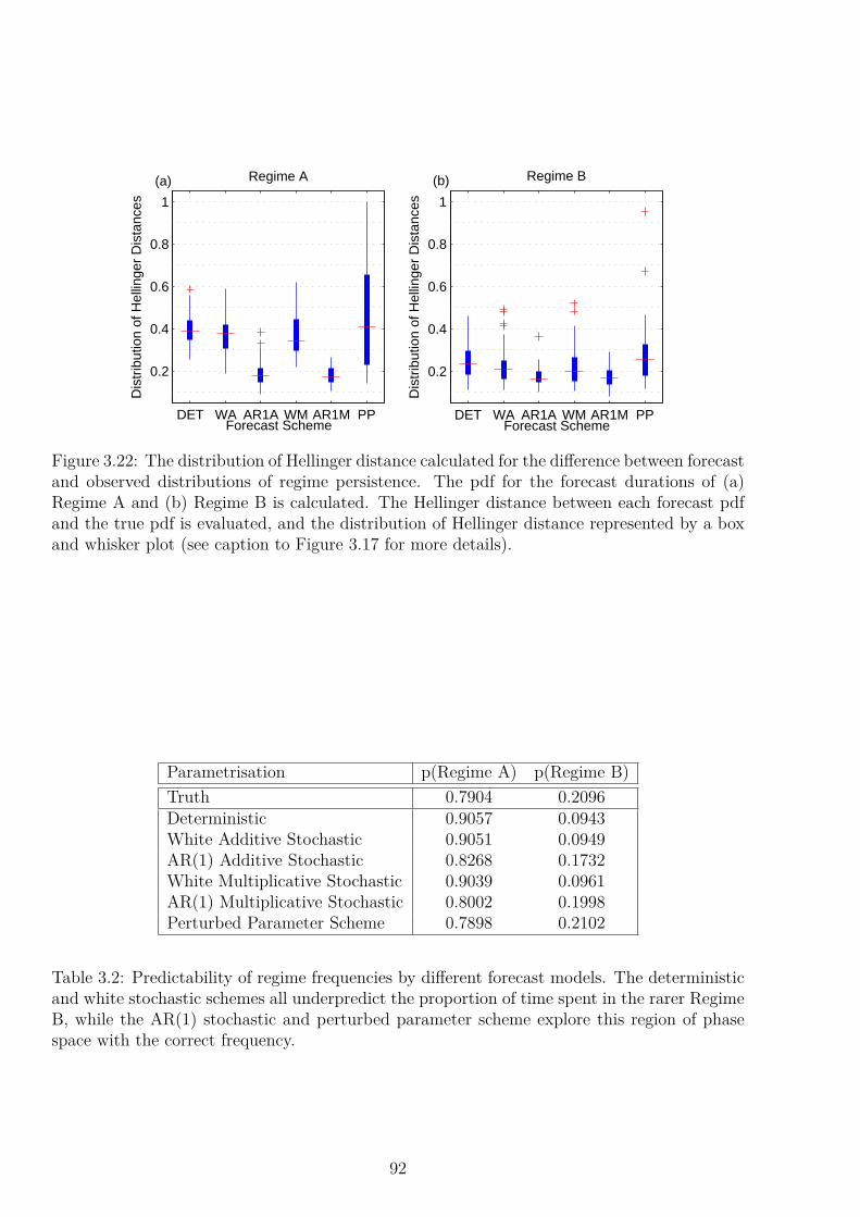
DET WA AR1A WM AR1M PP
0.2
0.4
0.6
0.8
1
Forecast Scheme
Regime A
Dis
trib
utio
n of
Hel
linge
r D
ista
nces
(a)
DET WA AR1A WM AR1M PP
0.2
0.4
0.6
0.8
1
Forecast Scheme
Regime B
Dis
trib
utio
n of
Hel
linge
r D
ista
nces
(b)
Figure 3.22: The distribution of Hellinger distance calculated for the difference between forecastand observed distributions of regime persistence. The pdf for the forecast durations of (a)Regime A and (b) Regime B is calculated. The Hellinger distance between each forecast pdfand the true pdf is evaluated, and the distribution of Hellinger distance represented by a boxand whisker plot (see caption to Figure 3.17 for more details).
Parametrisation p(Regime A) p(Regime B)
Truth 0.7904 0.2096Deterministic 0.9057 0.0943White Additive Stochastic 0.9051 0.0949AR(1) Additive Stochastic 0.8268 0.1732White Multiplicative Stochastic 0.9039 0.0961AR(1) Multiplicative Stochastic 0.8002 0.1998Perturbed Parameter Scheme 0.7898 0.2102
Table 3.2: Predictability of regime frequencies by different forecast models. The deterministicand white stochastic schemes all underpredict the proportion of time spent in the rarer RegimeB, while the AR(1) stochastic and perturbed parameter scheme explore this region of phasespace with the correct frequency.
92
3.4 Conclusion
The same stochastic parametrisation schemes presented in Chapter 2 are tested for their ability
to reproduce the climate of the Lorenz ’96 (L96) system. Two definitions of climate are
considered. The first defines the climate to be the pdf of the X variables, and the difference
between the forecast and true climate is evaluated using the Hellinger distance. According
to this measure, including white noise into the parametrisation scheme does not significantly
improve the climatology over that of a deterministic parametrisation scheme. This result is
observed for all noise models tested in both the c = 4 and c = 10 L96 cases. However, a
large, highly significant improvement in skill is observed when temporally autocorrelated noise
is used in the stochastic parametrisation schemes for both the c = 4 and c = 10 case.
It was found that the climatological skill of the forecast models is correlated with the
performance of the forecast model in weather prediction mode, in particular, with the reliability
of short-range forecasts. The correlation between the short term predictive skill of the forecast
model and its ability to reproduce the climatology of the L96 system provides support for
the “Seamless Prediction” paradigm. This provides a method of verifying climate predictions:
the climate model can be evaluated in weather forecasting mode to indicate the potential for
climatological skill.
The climate of the perturbed parameter forecast models described in Chapter 2 was also
tested. For the c = 10 case, the measured perturbed parameter model showed an improved
climatology over the deterministic and white noise stochastic models, but a significantly poorer
climatology than the red noise stochastic models, when the climate of the L96 system is defined
as the pdf of the X variables. However, for the c = 4 case, the perturbed parameter model
is not significantly different to any of the red noise stochastic models, and has a significantly
improved climatology over the deterministic and white noise schemes.
Regime behaviour, commonly observed in the atmosphere, is also observed in the L96
system. It is argued that the L96 system has two regimes for c = 10 and F = 20 — the
system is in Regime A 79% of the time, while the less common Regime B occurs 21% of
the time. The regime behaviour of this system makes it a useful testbed for analysing the
ability of different forecast models to reproduce regime behaviour. Three types of models were
considered: a deterministic parametrisation scheme, stochastic parametrisation schemes with
additive or multiplicative noise, and a perturbed parameter ensemble.
93

Each forecasting scheme was tested on its ability to reproduce the attractor of the full
system, defined in a reduced space based on an EOF decomposition of the truth time series.
None of the forecast models accurately capture the less common Regime B, though a significant
improvement is observed over the deterministic parametrisation when a temporally correlated
stochastic parametrisation is used instead. The stochastic parametrisation enables the system
to explore a larger portion of the attractor, in the same way in which a ball–bearing in a
potential well will explore around its equilibrium position when subjected to a random forcing.
The regime statistics describing the persistence of the regimes and their frequency of occurrence
were also improved for the stochastic parametrisations with AR(1) noise compared to the
deterministic scheme, and multiplicative noise was found to be particularly skilful.
The attractor for the perturbed parameter ensemble improves on that forecast by the
deterministic or white additive schemes; it shows a distinct peak in the attractor corresponding
to Regime B, though this peak is more pronounced than in the truth attractor. The ensemble
is also very skilful at forecasting the correct statistics for the regime behaviour of the system.
However, the 40 constituent members of the perturbed parameter ensemble differ greatly from
the true attractor, with many only showing one dominant regime with very rare transitions.
It is interesting that, while each individual ensemble member models the regime behaviour
poorly, when averaged together, the ensemble performs very well.
Using regime behaviour to study the climate of a system provides considerably more in-
formation than studying the pdf of the system. The pdf of the perturbed parameter ensemble,
while not as skilful as the red noise stochastic parametrisations, shows skill for the c = 10 case.
The pdfs of individual ensemble members are also all skilful, with a mean Hellinger distance
of 0.06 ± 0.03 (not shown) — all perturbed parameter ensemble members have a reasonable
pdf. However, the regime behaviour of the individual perturbed parameter ensemble members
varies widely. In order to correctly simulate the statistics of the weather (for example, the dur-
ation of blocking events over Europe), a climate simulator must accurately represent regime
behaviour. It is therefore important that climate models are explicitly tested on this ability.
The results presented here indicate that while the average of a perturbed parameter ensemble
performs well, individual ensemble members are at risk of failing this test.
94

4
Evaluation of Ensemble Forecast
Uncertainty: The Error-Spread Score
It is far better to foresee even without certainty than not to foresee at all.
– Henri Poincare
4.1 Introduction
The first and arguably most important lesson in any experimental physics course is that a
physicist must quantify the uncertainty in his or her measurement or prediction. Firstly, this
allows for comparison of measurement with theory: a theory can only be discounted if it predicts
a value outside of the “error bars” of a measurement. Additionally, a theory does not necessarily
predict a single value. For example, for the famous experiment in which electrons are fired one
at a time through a double-slit, the theory of quantum mechanics predicts the probability of
an electron striking a screen behind the slit at any given point. The statistical reliability of
the forecast pdf can only be verified by repeated measurements which then provide evidence
for the validity of the theory; many individual electrons were passed through the double slit,
and an interference pattern observed as predicted (Donati et al., 1973).
The same lesson is valid in the atmospheric sciences. A weather or climate prediction
should include an estimate of the uncertainty of the prediction. In weather forecasting, En-
semble Prediction Systems (EPS) are commonly used to give an estimate of error in a forecast;
the ensemble of forecasts is assumed to sample the full forecast uncertainty. As outlined in
95

Section 1.3, there are two main sources of uncertainty which must be represented in a weather
forecast, initial condition uncertainty and model uncertainty (Palmer, 2001).
Having attempted to represent the errors in our prediction, the accuracy of the forecast pdf
must be verified. In the same way that Donati et al. (1973) measured the location of many
electrons, many forecast-observation (or -verification) pairs must be used to evaluate how well
the forecast ensemble represents uncertainty. Ideally, the ensemble forecast should behave like
a random sample from the forecast pdf (the hypothetical pdf representing the uncertainty in
the forecast). The consistency condition is that the verification also behaves like a sample from
that pdf (Anderson, 1997; Wilks, 2006). If this condition is fulfilled, the ensemble is perfectly
capturing the uncertainty in the forecast.
In this chapter, techniques for evaluation of the predicted uncertainty in a forecast are
considered in the context of predicting the weather. In Section 4.2, the problems with current
methods of forecast verification are discussed, and the need for a new scoring rule, the Error-
spread Score, is motivated, which is defined in Section 4.3. The new Error-spread Score is shown
to be proper in Section 4.4, and in Section 4.5 the decomposition of the score into reliability,
resolution and uncertainty components is discussed. In Section 4.6 the Error-spread Score is
tested and compared to existing diagnostics using forecasts made in the Lorenz ’96 system. In
Section 4.7 the Error-spread Score is tested using operational ensemble forecasts from ECMWF.
The decomposition of the score is evaluated for the ECMWF forecasts in Section 4.8, which
gives a more complete understanding of the new score. Finally, in Section 4.9 the score is
used to evaluate forecasts made using the ECMWF seasonal forecasting system, and some
conclusions are drawn in Section 4.10.
4.2 Evaluation of Ensemble Forecasts
Section 1.7 outlined some of the different methods commonly used for forecast verification.
All the methods discussed are sensitive to the two properties which a probabilistic forecast
must have to be useful: reliability and resolution. Graphical forecast diagnostics provide a
comprehensive summary of the forecast, including an indication of reliability and resolution.
However, they do not produce an unambiguous ranking of forecasts, so it is difficult to use them
to compare many models. Scoring rules are useful as they provide a quantitative indication of
forecast skill, allowing many different forecasts to be compared. Brocker (2009) showed that all
96

strictly proper scores can be explicitly decomposed into a component which tests reliability and
a component which tests resolution. The decomposition also includes a third term, uncertainty,
which depends only on the statistics of the observations.
Currently, many scoring rules used for forecast verification, such as the Continuous Ranked
Probability Score, CRPS (Wilks, 2006), and the Ignorance Score, IGN (Roulston and Smith,
2002), require an estimate of the full forecast pdf. This is usually achieved using kernel smooth-
ing estimates or by fitting the parameters in some predetermined distribution, both of which
require certain assumptions about the forecast pdf to be made. Alternatively, the pdf must be
discretised in some way, such as for the Brier Score, BS and Ranked Probability Score, RPS
(Wilks, 2006), which were both originally designed for multi-category forecasts. On the other
hand, the RMS error-spread graphical diagnostic used in Chapter 2 is an attractive verifica-
tion tool as it does not require an estimation of the full forecast pdf, and instead is calculated
using the raw ensemble forecast data. However, being a graphical diagnostic, it is very difficult
to compare many forecast models using this tool (for example, comparing the many differ-
ent forecasts generated by changing the tunable parameters in a stochastic parametrisation
scheme).
A new scoring rule is proposed designed for ensemble forecasts of continuous variables,
that is particularly sensitive to the reliability of a forecast and which seeks to summarise the
RMS error-spread graphical diagnostic. In a similar way to the RMS error-spread graphical
diagnostic, it is formulated with respect to moments of the forecast distribution, and not
using the full distribution itself. These moments may be calculated directly from the ensemble
forecast, provided it has sufficient members for an accurate estimate to be made. The new
score proposed does not require the forecast to be discretised, and acknowledges the inability
of the forecaster to fully specify a probability distribution for a variable due to the amount
of information needed to estimate the distribution. This limitation has been recognised by
other authors and forms the basis for the development of Bayes Linear Statistics (Goldstein
and Wooff, 2007).
The new score will be compared with a number of existing proper scores: the Brier Score,
BS (1.14), the reliability component of the Brier Score, REL (1.17), the Ranked Probability
Score, RPS (1.20) and the Ignorance Score, IGN (1.21). Each score is converted into a Skill
Score by comparison with a reference forecast following (1.12).
97

4.3 The Error-Spread Score
Consider two distributions. Q(X) is the truth probability distribution function for variable X
which has moments mean, µ, variance, σ2, skewness, γ, and kurtosis1, β, defined in the usual
way:
µ = E[X], (4.1)
σ2 = E[(X − µ)2], (4.2)
γ = E
[(X − µ
σ
)3]
, (4.3)
β = E
[(X − µ
σ
)4]
, (4.4)
where E[·] denotes the expectation of the variable. The probabilistic forecast issued is denoted
P (X), with mean, m, variance, s2, skewness, g, and kurtosis, b, defined in the same way.
The perfect probabilistic forecast will have moments equal to those of the truth distribution:
m = µ, s2 = σ2, g = γ, and b = β, etc.
The proposed Error-spread Score, ES, is written
ES = (s2 − e2 − esg)2, (4.5)
where the difference between the verification, z, and the ensemble mean, m, is the error in the
ensemble mean,
e = m− z, (4.6)
and the verification, z, follows the truth probability distribution, Q. The mean value of
the score is calculated over many forecast-verification pairs, both from different grid point
locations and from different starting dates. A smaller average value of the score indicates a
better forecast.
The first two terms in the square of the right hand side of (4.5) are motivated by the error-
spread relationship (1.26): for a reliable ensemble, it is expected that the ensemble variance,
s2, will give an estimate of the expected squared error in the ensemble mean, e2 (Leutbecher,
1Note that kurtosis is used not excess kurtosis. The kurtosis of the normal distribution, βN = 3.
98
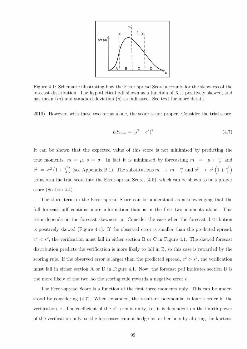
A B C D
m
s
X
pdf (X)
Figure 4.1: Schematic illustrating how the Error-spread Score accounts for the skewness of theforecast distribution. The hypothetical pdf shown as a function of X is positively skewed, andhas mean (m) and standard deviation (s) as indicated. See text for more details.
2010). However, with these two terms alone, the score is not proper. Consider the trial score,
EStrial = (s2 − e2)2 (4.7)
It can be shown that the expected value of this score is not minimised by predicting the
true moments, m = µ, s = σ. In fact it is minimised by forecasting m = µ + γσ2
and
s2 = σ2(
1 + γ2
4
)
(see Appendix B.1). The substitutions m → m+ gs2
and s2 → s2(
1 + g2
4
)
transform the trial score into the Error-spread Score, (4.5), which can be shown to be a proper
score (Section 4.4).
The third term in the Error-spread Score can be understood as acknowledging that the
full forecast pdf contains more information than is in the first two moments alone. This
term depends on the forecast skewness, g. Consider the case when the forecast distribution
is positively skewed (Figure 4.1). If the observed error is smaller than the predicted spread,
e2 < s2, the verification must fall in either section B or C in Figure 4.1. The skewed forecast
distribution predicts the verification is more likely to fall in B, so this case is rewarded by the
scoring rule. If the observed error is larger than the predicted spread, e2 > s2, the verification
must fall in either section A or D in Figure 4.1. Now, the forecast pdf indicates section D is
the more likely of the two, so the scoring rule rewards a negative error e.
The Error-spread Score is a function of the first three moments only. This can be under-
stood by considering (4.7). When expanded, the resultant polynomial is fourth order in the
verification, z. The coefficient of the z4 term is unity, i.e. it is dependent on the fourth power
of the verification only, so the forecaster cannot hedge his or her bets by altering the kurtosis
99

of the forecast distribution. The first term with a non-constant coefficient is the z3 term,
indicating that skewness is the first moment of the true distribution which interacts with the
forecaster’s prediction. The forecast skewness is therefore important, and should appear in the
proper score. If the score were based on higher powers, for example motivated from (sn − en)2,
the highest-order moment required would be the (2n− 1)st moment2.
4.4 Propriety of the Error-Spread Score
A scoring rule must be proper in order to be a useful measure of forecast skill. The ES can
not be strictly proper as it is only a function of the moments of the forecast distribution — a
pdf with the same moments as the true pdf will score equally well. However, it is important
to confirm that the ES is a proper score.
To test for propriety, we calculate the expected value of the score, assuming the verification
follows the truth distribution (refer to Appendix B.2 for the full derivation).
E [ES] =(
(σ2 − s2) + (µ−m)2 − sg(µ−m))2
+ σ2 (2(µ−m) + (σγ − sg))2 + σ4(β − γ2 − 1) (4.8)
In order to be proper, the expected value of the scoring rule must be minimised when
the truth distribution is forecast. Appendix B.2 confirms that the truth distribution falls
at a stationary point of the score, and that this stationary point is a minimum. Therefore,
the scoring rule is proper, though not strictly proper, and is optimised by issuing the truth
distribution. Appendix B.2 also includes a second test of propriety, from Brocker (2009).
4.5 Decomposition of the Error-Spread Score
It is useful to decompose a score into its constituent components, reliability and resolution, as
it gives insight into the source of skill of a forecast. It allows the user to identify the strengths of
one forecasting system over another. Importantly, it indicates the characteristics of the forecast
which require improvement, providing focus for future research efforts. Many of the existing
scoring rules have been decomposed into their constituent components. The BS (Brier, 1950)
2Scores based on the magnitude of the error were also considered, for example, (|s| − |e|)2, but a proper
score could not be found.
100

has been decomposed in several ways (e.g. Sanders, 1963; Murphy, 1973, 1986). Similarly,
the CRPS can be decomposed into two parts scoring reliability and resolution/uncertainty
(Hersbach, 2000). Todter and Ahrens (2012) show that a generalisation of IGN can also be
decomposed into reliability, resolution and uncertainty components. In each of these cases, the
decomposition allows the source of skill in a forecast to be identified.
It is desirable to be able to decompose the ES into its constituent components as has been
carried out for the BS and CRPS. Appendix B.3 shows that the ES score, as a proper score,
can be decomposed into a reliability, resolution and uncertainty component:
ES =1
n
I∑
i=1
J∑
j=1
Ni,j
(s2i − e2
i,j)2
︸ ︷︷ ︸
a
+
(
sigje2i,j +Gi,j
)2
e2i,j
︸ ︷︷ ︸
b
− 1
n
I∑
i=1
J∑
j=1
Ni,j
(e2i,j − e2)2
︸ ︷︷ ︸
c
+ e2i,j
G2
i,j
e2i,j
− G
e2
2
︸ ︷︷ ︸
d
+1
n
n∑
k=1
(e2 − e2k)2 + e2
k
(
G
e2
)2
− 2e3k
G
e2
︸ ︷︷ ︸
e
. (4.9)
The first term evaluates the reliability of the forecast. This has two components, a and
b, which test the reliability of the ensemble spread and the reliability of the ensemble shape
respectively. Term a is the squared difference between the forecast variance and the observed
mean square error for that forecast variance. For a reliable forecast, these terms should be
equal (Leutbecher and Palmer, 2008; Leutbecher, 2010). The smaller the term a, the more
reliable the forecast spread. Term b is the squared difference between the measured shape
factor, Gi,j, and the expression the shape factor takes if the ensemble spread and skew are
accurate, −sigje2i,j (B.41). If the forecast skewness, or ‘shape’, of the probability distribution
is a good indicator of the skewed uncertainty in the forecast distribution, this term will be
small. For both terms a and b, the sum is weighted by the number of forecast-verification
pairs in each bin, Ni,j.
The second term evaluates the resolution of the forecast. This also has two components, c
and d, testing the resolution of the predicted spread and the resolution of the predicted shape
respectively. Both terms evaluate how well the forecasting system is able to distinguish between
101
situations with different forecast uncertainty characteristics. Term c is the squared difference
between the mean square error in each bin and the climatological mean squared error. If the
forecast has high resolution, the spread of the forecast should separate predictions into cases
with low uncertainty (low mean square error), and those with high uncertainty (high mean
square error), resulting in a large value for term c. If the forecast spread does not indicate
the expected error in the forecast, term c will be small as all binned mean squared errors
will be close to the climatological value. Therefore a large absolute value of term c indicates
high resolution in the predicted spread. This is subtracted when calculating the Error-spread
Score, contributing to the low value of ES for a skilful forecast. Similarly, term d indicates the
resolution of the skewness or shape of the ensemble forecast, evaluating the squared difference
between the binned and climatological shape factors. If this term is large, the forecast has
successfully distinguished between situations with different degrees of skewness in the forecast
uncertainty: it has high shape resolution. Again, for both terms c and d, the sum is weighted
by the number of forecast-verification pairs in each bin.
The last term, e, is the uncertainty in the forecast, which is not a function of the binning
process. It depends only on the measured climatological error distribution, compared to the
individual measurements. Nevertheless, unlike for the Brier score decomposition, this term
is not independent of the forecast system, and instead provides information about the error
characteristics of the forecast system: a system with larger errors on average will have a larger
uncertainty term. The term is reduced by reducing the mean square error in the forecast.
4.6 Testing the Error-Spread Score: Evaluation of Fore-
casts in the Lorenz ’96 System
The experiments carried out in the L96 simplified model of the atmosphere described in
Chapter 2 can be used to test the ES. Forecasts made using the additive stochastic paramet-
risation scheme are evaluated at a lead time of 0.9 model time units (∼ 4.5 atmospheric days).
The other experimental details are identical to Chapter 2, including the details of the paramet-
risation scheme, and the number of ensemble members. The tunable parameters in the forecast
model, the magnitude of the noise term (σn) and the temporal autocorrelation of the noise
term (φ), are varied, and the forecasts for each evaluated using three techniques. Figure 4.2(a)
102
shows the graphical error-spread diagnostic (Section 1.7.3.1). The forecast-verification pairs
are binned according to the variance of the forecast. The average variance in each bin is plot-
ted against the mean square error in each bin. For a reliable forecast system, these points
should lie on the diagonal (Leutbecher and Palmer, 2008). Figure 4.2(b) shows the reliability
component of the Brier Score, REL (1.17), where the “event” was defined as “the Xk variable
is in the top third of its climatological distribution”. Figure 4.2(c) shows the new Error-spread
Skill Score (ESS), which is calculated with respect to the climatological forecast.
The difficulty of analysing many forecasts using a graphical method can now be appreciated.
Trends can easily be identified in Figure 4.2(a), but the best set of parameter settings is hard
to identify. The stochastic forecasts with small magnitude noise (low σn) are under-dispersive.
The error in the ensemble mean is systematically larger than the spread of the ensemble, i.e.
they are overconfident. However, the stochastic parametrisations with very persistent, large
magnitude noise (large σn, large φ) are over dispersive and under-confident. Figure 4.2(b)
shows REL evaluated for each parameter setting, which is small for a reliable forecast. It
scores highly those forecasts where the variance matches the mean square error, such that
the points in (a) lie on the diagonal. The ESS is a proper score, and is also sensitive to the
resolution of the forecast. It rewards well calibrated forecasts, but also those which have a
small error. The peak of the ESS in Figure 4.2(c) is shifted down compared to REL, and it
penalises the large σn, large φ models for the increase in error in their forecasts. The ESS
summarises Figure 4.2(a), and shows a sensitivity to both reliability and resolution as required
of a proper score.
4.7 Testing the Error-Spread Score: Evaluation of Medium-
Range Forecasts
The ESS was tested using ten day operational forecasts made with the ECMWF EPS. The
EPS uses a spectral atmospheric model, the Integrated Forecasting System (IFS) (described in
detail in Section 5.2). The EPS is operationally run out to day ten with a horizontal triangular
truncation of T6393, with 62 vertical levels, and uses persisted sea surface temperature (SST)
3The IFS is a spectral model, and resolution is indicated by the wave number at which the model is truncated.For comparison, a spectral resolution of T639 corresponds to 30 km resolution, or a 0.28o latitude/longitudegrid at the equator.
103

0 20 400
20
40
MS Spread
MS
Err
or
0 20 40 0 20 40 0 20 40 0 20 40 0 20 40
0
20
400
20
400
20
400
20
400
20
40(a)
0.0010.003
0.003
0.005
0.005
0.001
0.007
0.009
0.003
φ
σ / σ
mea
s
0.00
0
0.60
7
0.88
2
0.96
9
0.99
3
0.99
8
(b)
0.0
0.5
1.0
1.5
2.0
2.50.760.780.8
0.82
0.840.860.88
0.9
0.9
0.9
0.92
0.92
0.920.94
0.94
0.94
φ
σ / σ
mea
s
0.00
0
0.60
7
0.88
2
0.96
9
0.99
3
0.99
8
(c)
0.0
0.5
1.0
1.5
2.0
2.5
0.607 0.882 0.969 0.993 0.9980.000φ
2.5
2.0
1.5
1.0
0.5
0.0
σ / σm
Figure 4.2: (a) The Mean Square (MS) Error-Spread diagnostic, (b) the Reliability componentof the Brier Score and (c) the Error-spread Skill Score, evaluated for forecasts of the L96 systemusing an additive stochastic parametrisation scheme. In each figure, moving Left–Right theautocorrelation of the noise in the forecast model, φ, increases. Moving Bottom–Top, thestandard deviation of the noise, σn, increases. The individual figures in (a) correspond todifferent values of (φ, σm). The bottom row of figures in (a) are blank because deterministicforecasts cannot be analysed using the MS Error-Spread diagnostic: there is no forecast spreadto condition the binning on.
104

0 4.5 9 13.5 18 22.5289
290
291
292
293
294
295
Longitude
T 8
50
(a) EPS: 4oN
0 4.5 9 13.5 18 22.5289
290
291
292
293
294
295
Longitude
(b) DD: 4oN
13.3 20 26.7 33.3 40 46.7
250
260
270
280
290
300
Longitude
(c) EPS: 53oN
13.3 20 26.7 33.3 40 46.7
250
260
270
280
290
300
Longitude
(d) DD: 53oN
Figure 4.3: The 4DVar analyses (black) of temperature at 850 hPa (T850) are compared tothe ten-day ensemble forecasts (grey) at 11 longitudes at 4oN for (a) the EPS and (b) the DDsystem, and at 11 longitudes at 53oN for (c) the EPS and (d) the DD system. The forecastsare initialised on 19th April 2012 for all cases. The horizontal black dashed lines correspondto the deciles of the climatological distribution of T850 at this latitude.
anomalies instead of a dynamical ocean model. The 50 member ensemble samples initial con-
dition uncertainty using the EDA system (Isaksen et al., 2010). The perturbations prescribed
by the EDA system are combined with perturbations from the leading singular vectors to
define an ensemble which represents the initial condition uncertainty well (Buizza et al., 2008).
The EPS system uses stochastic parametrisations to represent uncertainty in the forecast due
to model deficiencies. The 50 ensemble members differ as each uses a different seed for the
stochastic parametrisation schemes. Two stochastic parametrisation schemes are used: SPPT
(Section 1.4.3.1) and SKEB (Section 1.4.3.2).
Ten day forecasts are considered, initialised from 30 dates between April 14th and Septem-
ber 15th 2012, and separated from each other by five days. The high resolution 4D variational
(4DVar) analysis (T1279, 16 km) is used for verification. Both forecast and verification fields
are truncated to T159 (125 km) before verification. Forecasts of temperature at 850 hPa (T850
— approximately 1.5 km above ground level) are considered, and the ES evaluated as a function
of latitude.
For comparison, a perfect statistical probabilistic forecast is generated based on the high
resolution T1279 operational deterministic forecast. This is defined in an analogous way to
the idealised hypothetical forecasts in Leutbecher (2010). The error between the deterministic
forecast and the 4DVar analysis is computed for each ten day forecast, and the errors grouped
as a function of latitude. Each deterministic forecast is then dressed by adding a 50 member
ensemble of errors to the deterministic forecast, where the errors are drawn from this latit-
udinally dependent distribution. The error distribution does not include spatial or temporal
correlations. This dressed deterministic (DD) ensemble can be considered a “perfect statist-
ical” forecast as the error distribution is correct if averaged over all time. However, the error
105

0 1 2 30
1
2
3
RMS Spread
RM
S E
rror
(a)
0.2 0.4 0.6 0.8 1 1.20.2
0.4
0.6
0.8
1
1.2
RMS Spread
RM
S E
rror
(b)
2 4 61
2
3
4
5
6
RMS Spread
RM
S E
rror
(c)
Figure 4.4: RMS error-spread plot for forecasts made using the EPS (pale grey) and the DDsystem (dark grey). Ten day forecasts of T850 are considered for latitudes between (a) 18oSand 10oS, (b) 0oN and 8oN , and (c) 50oN and 60oN . The ensemble forecasts are sorted andbinned according to their forecast spread. The standard deviation of the error in the ensemblemean in each bin is plotted against the RMS spread for each bin. For a reliable ensemble,these should lie on the diagonal shown (Leutbecher and Palmer, 2008).
distribution is static: it does not vary from day to day as the predictability of the atmospheric
flow varies. A useful score should distinguish between this perfect statistical forecast and the
dynamic probabilistic forecasts made using the EPS.
An example ten day forecast using these two systems is shown in Figure 4.3 for 11 longitudes
close to the equator, and for 11 longitudes at mid-latitudes. The flow dependency of the
EPS is evident — the spread of the ensemble varies with position giving an indication of the
uncertainty in the forecast. The spread of the DD ensemble varies slightly, indicating the
sampling error for a 50 member ensemble.
Figure 4.4 shows the RMS error-spread diagnostic for three different latitude bands. On
average, the DD is perfectly reliable — the mean of the scattered points lies on the diagonal
for each case considered. However, the spread of the forecast does not indicate the error in the
ensemble mean. In contrast, the EPS forecasts contain information about the expected error
in the ensemble mean. The spread of the ESS is well calibrated, though at latitudes close to
the equator it is slightly under-dispersive (Figure 4.4(b)). At a lead time of ten days, the RMS
error between the deterministic forecast and the verification is higher than the RMS error in
the ensemble mean for the lower resolution EPS. This difference is greatest at mid-latitudes,
and can be observed in Figure 4.4(c).
Figure 4.5 shows the skill of the EPS forecasts calculated using three different proper
scores: ES, RPS and IGN. For each, the smaller the score, the better the forecast. The BS
was also calculated, but the results were very similar to the RPS and so are not shown here.
All scores agree that the skill of the EPS forecast is lower in mid-latitudes than at ±20o.
However, they disagree as to the skill of the forecast near the equator. The RPS and IGN
106

−80 −60 −40 −20 0 20 40 60 800
1
2
3
4
5
6
Latitude
Sco
reFigure 4.5: Forecasting skill of the EPS as a function of latitude using the ES (solid); IGNcalculated following Roulston and Smith (2002) (dot-dash), for ten events defined with respectto the deciles of the climatology; RPS dash, for ten events defined with respect to the decilesof the climatology. The ten day forecasts are compared with the 4DVar analysis for T850 andaveraged over 30 initial dates in Summer 2012. The scores have been scaled to allow them tobe displayed on the same axes: the ES by a factor of 1
300, and the RPS by a factor of 5.
indicate a reduced skill at the equator, whereas ES indicates a higher skill there than at mid-
latitudes. The cause of this difference is that at the equator the climatological variability is
much smaller than at midlatitudes, so the climatological deciles are closer together. This affects
the scores conditioned on the climatological percentiles (RPS, IGN), which do not account for
the spacing of the bins. At the equator, even if the forecast mean and verification are separated
by several bins, the magnitude of the error is actually small. It seems unreasonable to penalise
forecasts twice near the equator when calculating a skill score — the first time from the closer
spaced bins, and the second time by calculating the skill score with respect to a more skilful
climatological forecast. The ES score is not conditioned on the climatological percentiles, so
is not susceptible to this. It rewards forecasts made close to the equator for their small RMS
error when compared to forecasts made at other latitudes.
Figure 4.6 shows skill scores for the EPS forecast calculated with reference to the DD
forecast, using three different proper scores, ESS, RPSS and IGNSS. In each case, the skill
score SS is related to the score for the EPS, SEPS, and for the DD, SDD by:
SS = 1 − SEP S
SDD
. (4.10)
The higher the skill score, the better the scoring rule is able to distinguish between the dynamic
probabilistic forecast made using the EPS, and the statistical forecast using the DD ensemble.
107
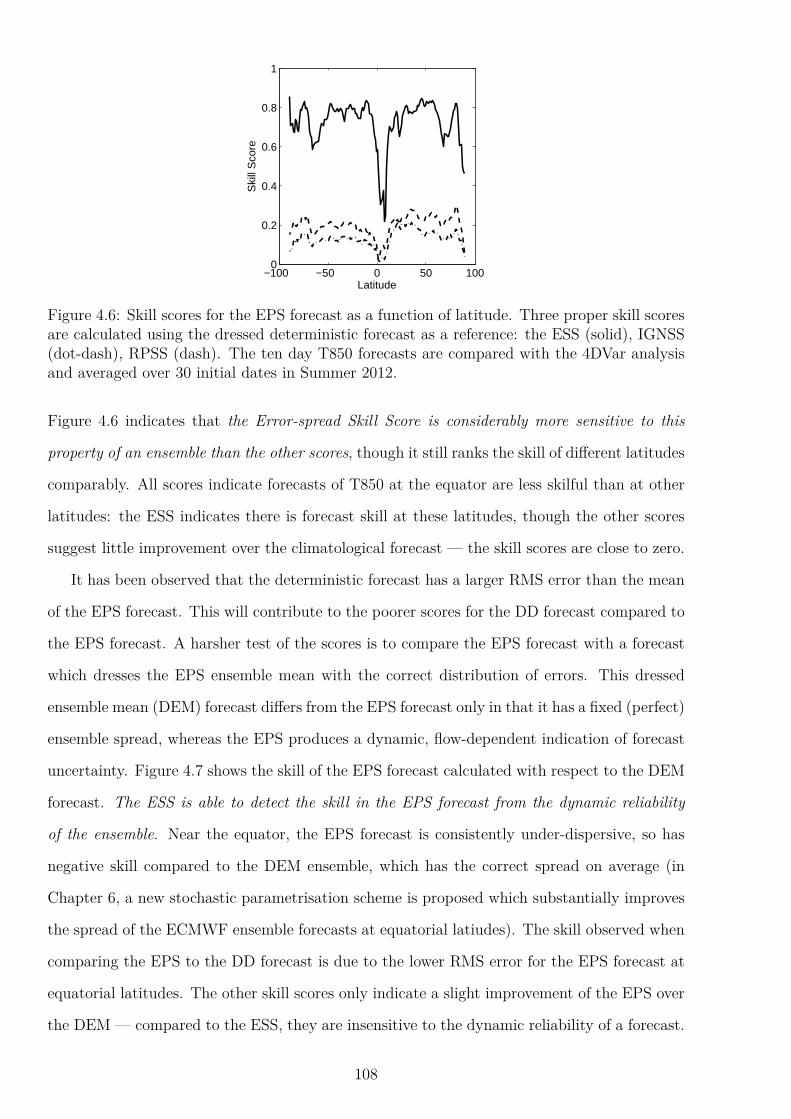
−100 −50 0 50 1000
0.2
0.4
0.6
0.8
1
Latitude
Ski
ll S
core
Figure 4.6: Skill scores for the EPS forecast as a function of latitude. Three proper skill scoresare calculated using the dressed deterministic forecast as a reference: the ESS (solid), IGNSS(dot-dash), RPSS (dash). The ten day T850 forecasts are compared with the 4DVar analysisand averaged over 30 initial dates in Summer 2012.
Figure 4.6 indicates that the Error-spread Skill Score is considerably more sensitive to this
property of an ensemble than the other scores, though it still ranks the skill of different latitudes
comparably. All scores indicate forecasts of T850 at the equator are less skilful than at other
latitudes: the ESS indicates there is forecast skill at these latitudes, though the other scores
suggest little improvement over the climatological forecast — the skill scores are close to zero.
It has been observed that the deterministic forecast has a larger RMS error than the mean
of the EPS forecast. This will contribute to the poorer scores for the DD forecast compared to
the EPS forecast. A harsher test of the scores is to compare the EPS forecast with a forecast
which dresses the EPS ensemble mean with the correct distribution of errors. This dressed
ensemble mean (DEM) forecast differs from the EPS forecast only in that it has a fixed (perfect)
ensemble spread, whereas the EPS produces a dynamic, flow-dependent indication of forecast
uncertainty. Figure 4.7 shows the skill of the EPS forecast calculated with respect to the DEM
forecast. The ESS is able to detect the skill in the EPS forecast from the dynamic reliability
of the ensemble. Near the equator, the EPS forecast is consistently under-dispersive, so has
negative skill compared to the DEM ensemble, which has the correct spread on average (in
Chapter 6, a new stochastic parametrisation scheme is proposed which substantially improves
the spread of the ECMWF ensemble forecasts at equatorial latiudes). The skill observed when
comparing the EPS to the DD forecast is due to the lower RMS error for the EPS forecast at
equatorial latitudes. The other skill scores only indicate a slight improvement of the EPS over
the DEM — compared to the ESS, they are insensitive to the dynamic reliability of a forecast.
108
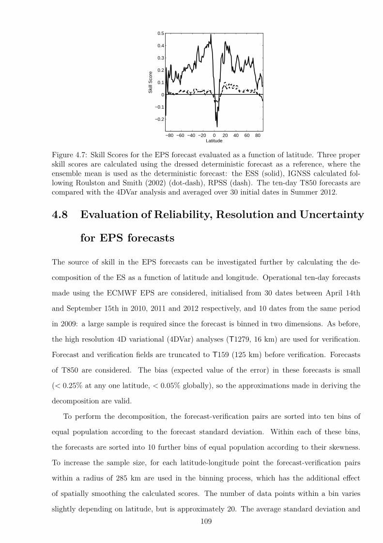
−80 −60 −40 −20 0 20 40 60 80
−0.2
−0.1
0
0.1
0.2
0.3
0.4
0.5
Latitude
Ski
ll S
core
Figure 4.7: Skill Scores for the EPS forecast evaluated as a function of latitude. Three properskill scores are calculated using the dressed deterministic forecast as a reference, where theensemble mean is used as the deterministic forecast: the ESS (solid), IGNSS calculated fol-lowing Roulston and Smith (2002) (dot-dash), RPSS (dash). The ten-day T850 forecasts arecompared with the 4DVar analysis and averaged over 30 initial dates in Summer 2012.
4.8 Evaluation of Reliability, Resolution and Uncertainty
for EPS forecasts
The source of skill in the EPS forecasts can be investigated further by calculating the de-
composition of the ES as a function of latitude and longitude. Operational ten-day forecasts
made using the ECMWF EPS are considered, initialised from 30 dates between April 14th
and September 15th in 2010, 2011 and 2012 respectively, and 10 dates from the same period
in 2009: a large sample is required since the forecast is binned in two dimensions. As before,
the high resolution 4D variational (4DVar) analyses (T1279, 16 km) are used for verification.
Forecast and verification fields are truncated to T159 (125 km) before verification. Forecasts
of T850 are considered. The bias (expected value of the error) in these forecasts is small
(< 0.25% at any one latitude, < 0.05% globally), so the approximations made in deriving the
decomposition are valid.
To perform the decomposition, the forecast-verification pairs are sorted into ten bins of
equal population according to the forecast standard deviation. Within each of these bins,
the forecasts are sorted into 10 further bins of equal population according to their skewness.
To increase the sample size, for each latitude-longitude point the forecast-verification pairs
within a radius of 285 km are used in the binning process, which has the additional effect
of spatially smoothing the calculated scores. The number of data points within a bin varies
slightly depending on latitude, but is approximately 20. The average standard deviation and
109

skewness are calculated for each bin, as are the average error characteristics required by (4.9).
The EPS is compared with the dressed ensemble mean (DEM) forecast described above.
The decomposition of the ES should distinguish between this perfect statistical forecast and
the dynamic probabilistic forecasts made using the EPS, and identify in what way the dynamic
probabilistic forecast improves over the perfect statistical case.
Figure 4.8(a) shows the forecasting skill of the EPS evaluated using the ES. The lower the
value of the score, the better the forecast. A strong latitudinal dependency in the value of the
score is observed, with better scores found at low latitudes. This can be attributed largely
to the climatological variability, which is strongly latitudinally dependent. At high latitudes
variability is greater, the mean square error is larger so the ES is larger. This is explained in
more detail in Section 4.7 above. Figure 4.8(b) shows the forecasting skill of the EPS evaluated
using the ES, where the ES has been calculated using the decomposition described in (4.9).
The results are similar to using the raw ES, confirming the decomposition is valid. The small
observed differences can be attributed to two causes. Firstly, the decomposition assumes that
spread and skew are discrete variables constant within a bin, which is not true. Secondly, the
decomposition uses neighbouring forecast-verification pairs to increase the sample size for the
binning process, which is not necessary when the ES is evaluated using (4.5). Figure 4.8(c)
shows the Error-spread Skill Score (ESS) calculated for the EPS with reference to the DEM
forecasts following (4.10). A positive value of the skill score indicates an improvement over
the DEM forecast whereas a negative value indicates the DEM forecast was more skilful. The
results overwhelmingly indicate the EPS is more skilful than the DEM, with positive scores
over much of the globe. The highest skill is found in two bands north and south of the equator
in the western Pacific Ocean. There are some small regions with negative skill over equatorial
land regions and over the equatorial east Pacific. It is these regions which are responsible for
the negative ESS at low latitudes in Figure 4.7.
To investigate the source of skill in the EPS compared to the DEM forecast, the decom-
position of the ES was calculated for both sets of forecasts. Figure 4.9 shows the reliability,
resolution and uncertainty terms calculated for the EPS (left hand column) and DEM (centre
column) forecasts. Visually, the plots in the two columns look similar. Comparing Figure 4.9(a)
and (b) indicates that the reliability term tends to be smaller for the EPS across much of the
tropics, and comparing (d) and (e) shows that the resolution term tends to be smaller for
110
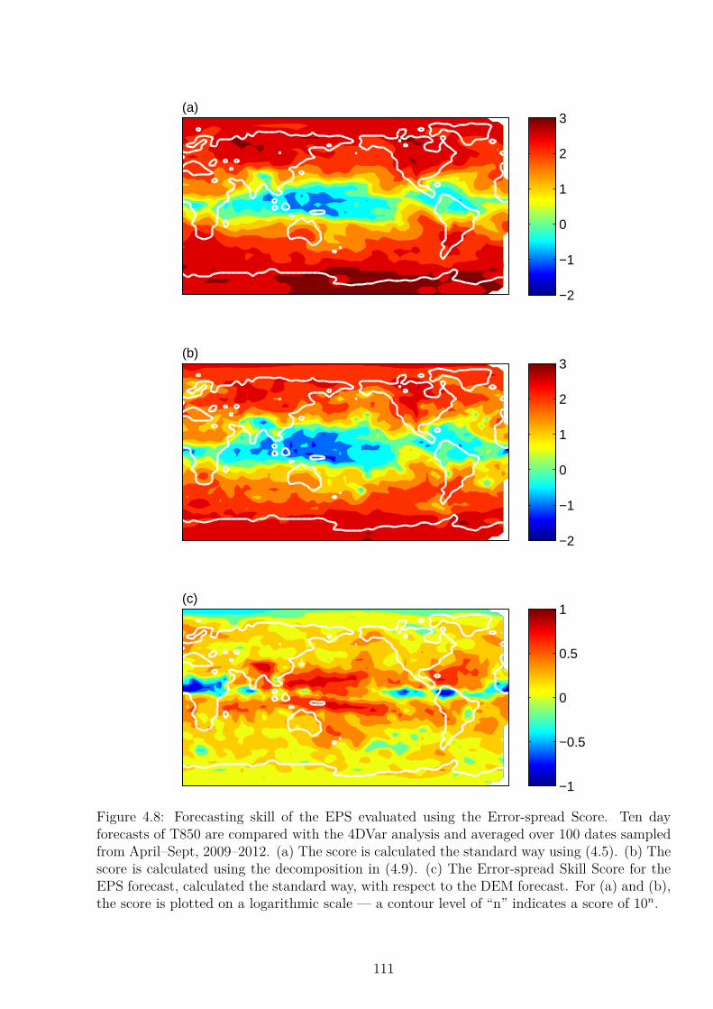
(a)
−2
−1
0
1
2
3
(b)
−2
−1
0
1
2
3
(c)
−1
−0.5
0
0.5
1
Figure 4.8: Forecasting skill of the EPS evaluated using the Error-spread Score. Ten dayforecasts of T850 are compared with the 4DVar analysis and averaged over 100 dates sampledfrom April–Sept, 2009–2012. (a) The score is calculated the standard way using (4.5). (b) Thescore is calculated using the decomposition in (4.9). (c) The Error-spread Skill Score for theEPS forecast, calculated the standard way, with respect to the DEM forecast. For (a) and (b),the score is plotted on a logarithmic scale — a contour level of “n” indicates a score of 10n.
111

the DEM. The uncertainty term, shown in (g) and (h), is similar for the EPS and DEM. In
Figure 4.9(b), the method of construction of the DEM forecast results in a strong horizontal
banding across much of the equatorial Pacific Ocean. The standard deviation of the DEM
forecast is constant as a function of longitude, and the error characteristics are similar, so the
reliability term is approximately constant.
To ease comparison, Figures 4.9 (c), (f) and (i) show the skill score calculated for the EPS
forecasts with reference to the DEM forecasts for the reliability, resolution and uncertainty
components of the ES respectively. Figure 4.9(c) shows the ES reliability skill score. High skill
scores indicate the EPS is more reliable than the DEM. Very high skill scores of greater than
0.8 are found in two bands north and south of the equator in the western Pacific Ocean, with
lower positive scores observed over much of the Pacific Ocean. This indicates that the high
skill in these regions, as indicated by the ESS, is largely attributable to an improvement in the
reliability of the forecast.
At polar latitudes and in the south east Pacific, the reliability skill score is negative, indic-
ating the DEM is more reliable than the EPS. However in these regions, Figure 4.9(f) shows a
ES resolution skill score that is large and negative. Because resolution contributes negatively
to the total score, a large value of resolution is desirable and negative values of the resolution
skill score indicate skill in the EPS forecast. At polar latitudes and in the south-east Pacific,
the EPS forecasts have more resolution than the DEM forecasts. Therefore, despite their low
reliability at these latitudes, the overall ESS indicates an improvement over the DEM. The
improvement in ES in these regions can be attributed to an improvement in resolution of the
forecast. At low latitudes, the resolution of the EPS is similar to that of the DEM.
Figure 4.9(i) shows the ES uncertainty skill score. This is zero over much of the globe,
indicating the EPS and DEM forecasts have very similar uncertainty characteristics. This is
as expected, since the forecast error characteristics are near identical. The small deviations
from zero can be attributed to sampling: the sample distribution of errors used to dress the
deterministic forecast does not necessarily have a mean of zero.
The ES decomposition has indicated in what ways the EPS forecast is more skilful than the
DEM forecast, and has also highlighted regions of concern. It is of interest to see if this skill
is reflected in other diagnostic tools. The calibration of the second moment of the ensemble
forecast can be evaluated by constructing RMS error-spread diagrams, which test whether
112

(a)
−2
−1
0
1
2
3
(b)
(d)
(e)
(g)
(h)
(c)
−1
−0.5
0
0.5
1
(f)
(i)
Figure 4.9: Source of forecasting skill evaluated using the ESS, comparing the EPS and DEMforecasts. See text for more details. The reliability component of (a) the EPS forecasts and(b) the DEM forecasts. (c) The reliability skill score: positive values indicate the EPS is morereliable than the DEM forecast. The resolution component of (d) the EPS forecasts and (e)the DEM forecasts. (f) The resolution skill score: negative values indicate the EPS has moreresolution than the DEM forecast. The uncertainty component of (g) the EPS forecasts and(h) the DEM forecasts. (i) The uncertainty skill score: positive values indicate the EPS haslower uncertainty than the DEM forecast. The colourbar in (a) also corresponds to figures (b),(d-e) and (g-h). The colourbar in (c) also corresponds to figures (f) and (i). In (a-b), (d-e)and (g-h), the components of the score are plotted on a logarithmic scale — a contour level of“n” indicates a score of 10n.
113
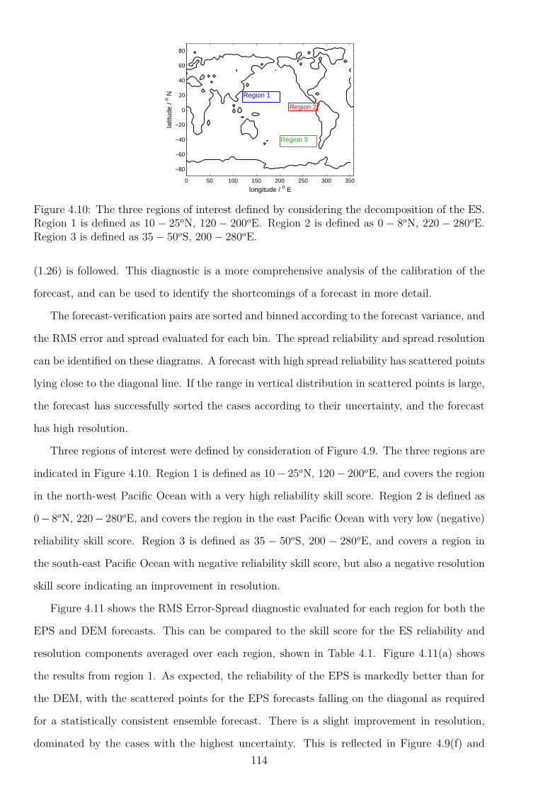
Region 1
Region 2
Region 3
longitude / o E
latit
ude
/ o N
0 50 100 150 200 250 300 350
−80
−60
−40
−20
0
20
40
60
80
Figure 4.10: The three regions of interest defined by considering the decomposition of the ES.Region 1 is defined as 10 − 25oN, 120 − 200oE. Region 2 is defined as 0 − 8oN, 220 − 280oE.Region 3 is defined as 35 − 50oS, 200 − 280oE.
(1.26) is followed. This diagnostic is a more comprehensive analysis of the calibration of the
forecast, and can be used to identify the shortcomings of a forecast in more detail.
The forecast-verification pairs are sorted and binned according to the forecast variance, and
the RMS error and spread evaluated for each bin. The spread reliability and spread resolution
can be identified on these diagrams. A forecast with high spread reliability has scattered points
lying close to the diagonal line. If the range in vertical distribution in scattered points is large,
the forecast has successfully sorted the cases according to their uncertainty, and the forecast
has high resolution.
Three regions of interest were defined by consideration of Figure 4.9. The three regions are
indicated in Figure 4.10. Region 1 is defined as 10 − 25oN, 120 − 200oE, and covers the region
in the north-west Pacific Ocean with a very high reliability skill score. Region 2 is defined as
0 − 8oN, 220 − 280oE, and covers the region in the east Pacific Ocean with very low (negative)
reliability skill score. Region 3 is defined as 35 − 50oS, 200 − 280oE, and covers a region in
the south-east Pacific Ocean with negative reliability skill score, but also a negative resolution
skill score indicating an improvement in resolution.
Figure 4.11 shows the RMS Error-Spread diagnostic evaluated for each region for both the
EPS and DEM forecasts. This can be compared to the skill score for the ES reliability and
resolution components averaged over each region, shown in Table 4.1. Figure 4.11(a) shows
the results from region 1. As expected, the reliability of the EPS is markedly better than for
the DEM, with the scattered points for the EPS forecasts falling on the diagonal as required
for a statistically consistent ensemble forecast. There is a slight improvement in resolution,
dominated by the cases with the highest uncertainty. This is reflected in Figure 4.9(f) and
114

0 1 20
0.5
1
1.5
2
RMS Spread
RM
S E
rror
(a)
0 1 20
0.5
1
1.5
2
RMS Spread
RM
S E
rror
(b)
1 2 3 4 51
2
3
4
5
RMS Spread
RM
S E
rror
(c)
Figure 4.11: RMS Error-Spread plot for forecasts made using the EPS (pale grey) and theDEM system (dark grey). Ten day forecasts of T850 are considered for three regions: (a)region 1: 10 − 25oN , 120 − 200oE, (b) region 2: 0 − 8oN , 220 − 280oE and (c) region 3:35 − 50oS, 200 − 280oE. The ensemble forecasts are sorted and binned according to theirforecast spread. The RMS error in each bin is plotted against the RMS spread for each bin.For a reliable ensemble, these should lie on the diagonal shown (Leutbecher and Palmer, 2008)
Region RELSS RESSS1 0.81 -0.482 -0.72 -0.393 -0.93 -1.19
Table 4.1: Skill scores for the reliability and resolution components of the ES (RELSS andRESSS respectively) for the ECMWF EPS forecast compared to the DEM forecast, for eachof the three regions defined in the text.
Table 4.1, which show an improvement in the region on average.
In Figure 4.11(b), the results are shown for region 2. The reliability of the EPS forecast
is indeed poorer than for the DEM forecast; the ensemble is consistently under-dispersive.
However, the figure indicates an improvement in resolution in this region. This improvement
can be traced to a tongue of very low resolution skill score extending north west from the
Peruvian coast, visible in Figure 4.9(f).
Figure 4.11(c) shows the results for region 3. As for region 2, the EPS forecast is less reliable
than the DEM forecast being somewhat underdisersive, though the difference is less great than
in region 2. The resolution of the EPS forecast is better than for the DEM forecast, as expected
from the ES decomposition. The ES decomposition has correctly identified regions of interest
for the ECMWF EPS which have particularly high or low skill with respect to the reliability or
resolution of the forecast. Investigating these regions further using more complete, graphical
tests of statistical consistency, can then indicate in what way the forecast is unreliable or has
poor resolution.
115

0 0.5 10
0.5
1 Month 1 : M
RMS Spread
RM
S E
rror
(a)
0 0.5 10
0.5
1Month 2−4: JJA
RMS Spread
RM
S E
rror
(b)
0 0.5 10
0.5
1Month 5−7: SON
RMS Spread
RM
S E
rror
(c)
0 0.5 10
0.5
1 Month 1 : N
RMS Spread
RM
S E
rror
(d)
0 0.5 10
0.5
1Month 2−4: DJF
RMS Spread
RM
S E
rror
(e)
0 0.5 10
0.5
1Month 5−7: MAM
RMS Spread
RM
S E
rror
(f)
Figure 4.12: RMS error-spread diagnostic for System 4 seasonal forecasts of SST initialised in(a–c) May and (d–e) November. Forecasts of the average SST over each season are considered,and compared to reanalysis. The upright dark grey triangles are for the Nino 3.4 region, theinverted mid-grey triangles are for the Equatorial Indian Ocean region, and the light greycircles are for the North Pacific region, where the regions are defined in the text. To increasethe sample size for this diagnostic, the unaveraged fields of SSTs in each region are used insteadof their regionally average value.
4.9 Application to Seasonal Forecasts
Having confirmed that the Error-spread Score is a proper score, sensitive to both reliability
and resolution, but that is particularly sensitive to the reliability of a forecast, the score can
be used to evaluate forecasts made with the ECMWF seasonal forecasting system, System 4.
In System 4, the IFS has a horizontal resolution of T255 (∼ 80 km grid) with 91 levels in the
vertical. The IFS is coupled to the ocean model, Nucleus for European Modelling of the Ocean
(NEMO), and a 51 member ensemble forecast is produced out to a lead time of seven months.
The forecasts are initialised from 1st May and 1st November for the period 1981–2010. These
seasonal forecasts were provided by Antje Weisheimer (ECMWF, University of Oxford).
Three regions are selected for this case study: the Nino 3.4 (N3.4) region is defined as
5oS−5oN , 120−170oW , the equatorial Indian Ocean (EqIO) region is defined as 10oS−10oN ,
50 − 70oE, and the North Pacific (NPac) region is defined as 30 − 50oN , 130 − 180oW . The
monthly and areally averaged SST anomaly forecasts are calculated for a given region, and
compared to the analysis averaged over that region. The forecasts made with System 4 are
compared to two reference forecasts. The climatological forecast is generated by calculating
the mean, standard deviation and skewness of the areally averaged reanalysis SST for each
116

M J J A S O N0
0.5
1
Month
ES
(a)
M J J A S O N0
0.02
0.04
0.06
Month
ES
(c)
M J J A S O N0
0.05
0.1
Month
ES
(e)
N D J F M A M0
0.5
1
Month
ES
(b)
N D J F M A M0
0.02
0.04
0.06
Month
ES
(d)
N D J F M A M0
0.05
0.1
Month
ES
(f)
Figure 4.13: The ES score as a function of lead time for forecasts of monthly averaged seasurface temperatures, averaged over each region. In each panel, the solid line with circlemarkers corresponds to the System 4 forecast, the solid line is for the climatological forecast,and the dashed line is for the persistence forecast. Panels (a)–(b) are for the Nino 3.4 region,(c)–(d) are for the Equatorial Indian Ocean region, and (e)–(f) are for the North Pacific region.The left (right) hand column is for forecasts initialised in May (November).
region over the 30 year time period considered. This forecast is therefore perfectly reliable,
though has no resolution. A persistence forecast is also generated. The mean of the persistence
forecast is set to the average reanalysis SST for the month prior to the start of the forecast (e.g.
April for the May initialised forecasts). The mean is calculated separately for each year, and
analysis increments calculated as the difference between the SST reanalysis and the starting
SST. The standard deviation and skewness of the analysis increments are calculated and used
for the persistence forecast.
Figure 4.12 shows the RMS error-spread diagnostic for each region calculated for each
season. The spread of the forecasts for each region gives a good indication of the expected
error in the forecast. However, it is difficult to identify which region has the most skilful
forecasts: the EqIO has the smallest error on average, but the forecast spread does not vary
greatly from the climatological spread. In contrast, the errors in the forecasts for the N3.4
region and the NPac region are much larger, but the spread of the ensemble also has a greater
degree of flow dependency.
Figure 4.13 shows the average ES score calculated for each region for the System 4 ensemble
forecasts (solid line with circles), for the climatological forecast (solid line) and for the persist-
117

ence forecast (dashed line) for the May and November start dates respectively. The System 4
forecasts for the EqIO (panels (c) and (d)) have the lowest (best) ES for the forecast period
for both start dates. However, this region shows little variability, so the climatological and
persistence forecasts are also very skilful. In the NPac region (panels (e) and (f)), variations
in SST are much greater, but show little long term signal: the ensemble is unable to forecast
the observed variations, so the ES is higher in this region. The climatological and persistence
forecasts are also poorer due to the high variability. System 4 forecasts for the N3.4 region also
have a high ES. However, the climatological and persistence forecasts score very poorly, and
have considerably higher ES than System 4 at all lead times for the May initialised forecasts,
and at some lead times for the November initialised cases. This indicates that there is consid-
erable skill in the System 4 forecasts for the N3.4 region: they contain significant information
over that in the climatological or persistence forecasts. For the November start date, the per-
sistence forecast is most skilful at short lead times though very poor at long lead times, and
the climatological forecast is most skilful for the longest lead times but very poor at short lead
times. The System 4 forecasts perform well throughout the time window.
Consideration of Figure 4.13 also indicates how the ES balances scoring reliability and
resolution in a forecast. Since the climatological and persistence forecasts are perfectly reliable
by construction, the difference in their scores is due to resolution. Figure 4.14 shows the spread
of each reference forecast as a function of lead time for all regions and both start dates. The
skill of the reference forecasts as indicated by Figure 4.13 can be seen to be directly linked
to their spread: the ES scores a reliable forecast with narrow spread as better than a reliable
forecast with large spread. The strong seasonal dependency of the variability of SSTs in the
N3.4 region explains the high skill of the climatological forecast for March–May, but low skill
at other times.
Figure 4.13 shows that the ES detects considerable skill in System 4 forecasts when com-
pared to the climatological or persistence forecasts, but that this skill is dependent on the
region under consideration and the time of year. The skill in the forecasts indicates that the
full forecast pdf gives a reliable estimate of the uncertainty in the ensemble mean, and varies
according to the predictability of the atmospheric flow.
118

M J J A S O N0.20.40.60.8
11.2
Month
σ
(a)
N D J F M A M0.20.40.60.8
11.2
Month
σ
(b)
M J J A S O N0.20.40.60.8
11.2
Month
σ
(c)
N D J F M A M0.20.40.60.8
11.2
Month
σ
(d)
M J J A S O N0.20.40.60.8
11.2
Month
σ(e)
N D J F M A M0.20.40.60.8
11.2
Month
σ
(f)
Figure 4.14: The standard deviation of the climatological (solid line) and persistence (dashedline) reference forecasts for SST, as a function of forecast lead time. The forecasts werecalculated using the analysis data over the time period analysed, 1981–2010. Panels (a)–(b) are for the Nino 3.4 region, (c)–(d) are for the Equatorial Indian Ocean region, and (e)–(f)are for the North Pacific region. The left (right) hand column is for forecasts initialised in May(November).
4.10 Conclusion
A new proper score, the Error-spread Score (ES), has been proposed for evaluation of ensemble
forecasts of continuous variables. It is unique as it is formulated purely with respect to moments
of the ensemble forecast distribution, instead of using the full distribution itself. This means
that the full forecast pdf does not need to be estimated or stored. It is suitable for evaluation of
continuous forecasts, and does not require the discretisation of the forecast using bins, as is the
case for the categorical Brier and Ranked Probability Scores. The score is designed to evaluate
how well a forecast represents uncertainty: is the forecast able to distinguish between cases
where the atmospheric flow is very predictable from those where the flow is unpredictable? A
well calibrated probabilistic forecast that represents uncertainty is essential for decision making,
and therefore has high value to the user of the forecast. The ES is particularly sensitive to
testing this requirement.
In a similar manner to other proper scores, the ES can be decomposed into reliability,
resolution and uncertainty components. The ES reliability component evaluates the reliability
of the forecast spread and skewness. This term is small if the forecast and verification are
119

statistically consistent, and the moments of the ensemble forecast are a good indication of the
statistical characteristics of the verification. Similarly, the ES resolution component evaluates
the resolution of the forecast spread and shape. This term contributes negatively to the ES,
so a large resolution term is desirable. This term is large if the spread and skewness of the
ensemble forecast vary according to the state of the atmosphere and the predictability of the
atmospheric flow. The spread of a forecast system with high ES resolution separates forecast
situations with high uncertainty (large mean square error) from those with low uncertainty. The
ES uncertainty component depends only on the measured (climatological) error distribution,
and is independent of the forecast spread or skewness. A forecast system with larger errors on
average will have a larger (poorer) uncertainty component.
The ESS was tested using forecasts made in the Lorenz ’96 system, and was found to
be sensitive to both reliability and resolution as expected. The score was also tested using
forecasts made with the ECMWF IFS. The score indicates that EPS forecasts, which have
a dynamic representation of model uncertainty, are considerably more skilful than a dressed
deterministic ensemble which does not have a flow dependent probability distribution. Existing
scores are not particularly sensitive to this characteristic of probabilistic forecasts. The ES
decomposition attributed the improvement in skill at low latitudes to an improvement in
reliability, whereas the skill at higher latitudes was due to an improvement in resolution. The
ES decomposition was used to highlight a number of regions of interest for the EPS, and the
RMS error-spread diagnostic was calculated for these regions. The results were as expected
from the ES decomposition, but also indicated in what way the forecast was reliable or showed
resolution. The decomposition shown in this chapter is therefore a useful tool for analysing
the source of skill in ensemble forecasts, and for identifying regions which can be investigated
further using more comprehensive graphical diagnostic tools.
The ESS was used to evaluate the skill of seasonal forecasts made using the ECMWF
System 4 model. The score indicates significant skill in the System 4 forecasts of the Nino
3.4 region, as the ensemble is able to capture the flow-dependent uncertainty in the ensemble
mean. The results indicate that the ESS is a useful forecast verification tool due to its ease of
use, computational cheapness and sensitivity to desirable properties of ensemble forecasts.
120

5
Experiments in the IFS:
Perturbed Parameter Ensembles
But as the cool and dense Air, by reason of its greater Gravity, presses upon the hot
and rarified, ’tis demonstrated that this latter must ascend in a continued stream as
fast as it Rarifies
– Edmund Halley, 1686
5.1 Introduction
In Chapters 2 and 3, the impact of perturbed parameter and stochastic representations of model
uncertainty on forecasts in the L96 system was considered. The results from that simple system
indicated that the best stochastic parametrisations produced more skilful forecasts than the
perturbed parameter schemes. However, the perturbed parameter ensembles were skilful in
forecasting the weather of the system, and performed better than many of the sub-optimal
stochastic schemes, such as those which used white noise. This chapter will extend the earlier
work in the Lorenz ’96 system by comparing the performance of a stochastic and perturbed
parameter representation of model uncertainty in the ECMWF convection scheme. Convection
is generally acknowledged to be the parametrisation to which weather and climate models
are most sensitive (Knight et al., 2007), and it is therefore imperative that the uncertainty
originating in the parametrisation of convection is well represented.
In Section 5.2, the ECMWF model, the Integrated Forecasting System (IFS), is described,
121

and its parametrisation schemes are outlined. In Section 5.3, a generalisation to SPPT is
formulated which allows the stochastic perturbations to the convection tendency to be turned
off and replaced with alternative schemes. Section 5.4 describes the perturbed parameter
representations of model uncertainty which have been developed for this study. In Section 5.5,
the experimental procedure and verification techniques are described, and results are presented
in Section 5.6. In Section 5.7, the results are discussed and some conclusions are drawn.
5.2 The Integrated Forecasting System
The IFS is the operational global weather forecasting model developed and operated by
ECMWF. The following description refers to model version CY37R2, and the configuration
which was operational in 2011. The IFS comprises several components (Anderson and Persson,
2013; ECMWF, 2012). The atmospheric general circulation model consists of diagnostic
equations describing the physical relationship between pressure, density, temperature and
height, together with prognostic equations describing the time evolution of horizontal wind
speed (zonal, U, and meridional, V), temperature (T), humidity (q), and surface pressure. The
model dynamical equations describe the evolution of the resolved-scale variables, while the ef-
fect of sub-grid scale processes is included using physically motivated, but statistically derived,
parametrisation schemes. The atmospheric model contains a number of these parametrisation
schemes, which will be discussed further in Section 5.2.1. Each scheme operates independently
on each atmospheric vertical column. Two stochastic parametrisation schemes can be used to
represent model uncertainty: SPPT (Section 1.4.3.1) and SKEB (Section 1.4.3.2).
The atmospheric model is numerically integrated using a semi-Lagrangian advection scheme
combined with a semi-implicit time integration scheme. Together, these provide stability and
accuracy, enabling the use of larger time steps to reduce integration time. Horizontally, the IFS
is a dual spectral/grid-point model. The dynamical variables are represented in spectral space
to aid the calculation of horizontal derivatives and the time-stepping scheme. The physical
parametrisations are spatially localised, so are implemented in grid-point space on a reduced
Gaussian grid. The model then converts back and forth between grid-point and spectral space.
Vertically, the atmospheric model is discretised using sigma co-ordinates. This is a hybrid
co-ordinate system; near the surface, the sigma levels follow the orographic contours whereas
higher in the atmosphere the sigma levels follow surfaces of constant pressure.
122

Physics Parametrisation Scheme AbbreviationRadiation RDTTTurbulence and Gravity Wave Drag TGWDNon-orographic Gravity Wave Drag NOGWConvection CONVLarge Scale Water Processes LSWP
Table 5.1: Physical parametrisation schemes in the IFS atmospheric model
The atmospheric model is coupled to a land surface model — the H-TESSEL scheme
(Hydrology-Tiled ECMWF Scheme for Surface Exchange over Land). The land within each
grid box is represented by up to six different types of surface, with which the atmosphere
exchanges water and energy. The atmospheric model is also coupled to an ocean wave
model called “WAM”. The coupling allows the exchange of energy between wind and waves
in both directions. Persisted SST anomalies are used out to day ten; the atmosphere and the
ocean are coupled through exchanges of heat, momentum and mass.
Data assimilation is used to calculate the starting conditions for the IFS forecasts. The
four-dimensional variational data assimilation (4DVar) system combines information from ob-
servations with the physical description of the atmosphere contained in the model. This gen-
erates a physically reasonable estimate of the state of the atmosphere. However, this method
produces no flow-dependent estimate of the uncertainty in the analysis. To estimate this, an
ensemble of data assimilations (EDA) is generated: ten equally likely analyses are calculated at
a resolution of T399 (Isaksen et al., 2010). They differ from each other due to the introduction
of small perturbations in the observations and SST, as well as perturbations from SPPT.
Operationally, the model is used to produce both a high resolution deterministic forecast
and a lower resolution ensemble forecast out to a lead time of fifteen days. The deterministic
model is run at a spectral resolution of T1279 (16 km) with 91 levels in the vertical and a time
step of 10 minutes. A single forecast is made using unperturbed initial conditions from the
4DVar system, without the SPPT and SKEB parametrisation schemes in the forecast model.
The EPS is operationally run with a spectral resolution of T639 (30 km) and 62 vertical levels,
and with a time step of 20 minutes. The ensemble has fifty perturbed members and one
control member. Initial condition uncertainty is sampled using the EDA system, combined
with perturbations from the leading singular vectors. The stochastic parametrisations are
activated to sample model uncertainty.
123
5.2.1 Parametrisation Schemes in the IFS
There are five main parametrisation schemes in the IFS, shown in Table 5.1. The physics tend-
encies from these five schemes are combined with the dynamical tendencies using a technique
called “fractional stepping” (Wedi, 1999). The schemes are called sequentially, and schemes
called later use updated variables. This has the disadvantage of introducing intermediate time
steps (hence “fractional stepping”) at which the tendencies are updated by each parametrisa-
tion scheme in turn. However, it has the advantage of ensuring a balance between the different
physical parametrisation schemes.
The first scheme to be called is the radiation scheme (RDTT), including both a long- and
short-wave radiation calculation. The full radiation scheme is very expensive, so it is calcu-
lated on a coarser grid than the other parametrisation schemes, and the resultant tendencies
interpolated to the required resolution. Furthermore, the scheme is not run at every time step:
for the high resolution forecast, it is run once an hour, and for the EPS it is run once every
three hours. The radiation scheme interacts with clouds: incoming short wave radiation is
reflected by clouds, and the clouds emit long wave radiation. Since 2007, the Monte Carlo
Independent Column Approximation (McICA) approach has been used to account for clouds.
The grid box is divided into a number of sub-columns, each of which has a cloud fraction of ‘0’
or ‘1’ at each vertical level. Instead of calculating the sum over all columns in a grid box and
over all radiation intervals (which would be prohibitively expensive), a Monte Carlo approach
is used whereby the radiative transfer calculation is performed for a single randomly selected
sub column only. This will introduce unbiased random errors into the solution.
The second scheme called accounts for vertical exchange of energy, momentum and moisture
due to turbulence and gravity wave drag (TGWD). The scheme accounts for turbulent exchange
between the surface and the lowest atmospheric levels. Atmospheric momentum is also affected
by sub-grid scale orography. Orography exerts a drag on the atmospheric flow both from
blocking the flow in the lowest levels, and due to reflection and absorption of gravity waves.
The third scheme is the non-orographic gravity wave drag scheme (NOGW). Non-orographic
gravity waves are generated by convection, the jet stream and frontogenesis. They are par-
ticularly important in the stratosphere and mesosphere, where they contribute to driving the
Brewer-Dobson circulation, and the quasi-biennial and semi-annual oscillations.
The convection parametrisation (CONV) is based on the mass-flux scheme of Tiedtke
124

(1989). The scheme describes three types of convective cloud: deep, shallow and mid-level. The
convective clouds in a column are represented by a pair of entraining and detraining plumes
of a given convective type, which describe updraft and downdraft processes respectively1. The
choice of convective type determines certain properties of the cloud (such as the entrainment
formulation). The mass flux at cloud base for deep convection is estimated by assuming that
deep convection acts to reduce convectively available potential energy (CAPE) over some spe-
cified (resolution dependent) time scale. Mid-level convection occurs at warm fronts. The
mass flux at cloud base is set to be the large scale vertical mass flux at that level. For shallow
convection, the mass flux at cloud base is derived by assuming that the moist static energy in
the sub-cloud layer is in equilibrium.
Finally, the large scale water processes (LSWP, or “cloud”) scheme contains the prognostic
equations for cloud liquid water, cloud ice, rain, snow and cloud fraction. It builds on the
scheme of Tiedtke (1993), but is a more complete description, including more prognostic vari-
ables and an improved representation of mixed phase clouds. Whereas the convection scheme
calculates the effect of unresolved convective clouds, the cloud scheme calculates the impact of
clouds which are resolved by the model. This means that the same cloud could be represented
by a different parametrisation scheme if the resolution of the model changed.
The IFS also contains parametrisations of methane oxidation and ozone chemistry. The
tendencies from these schemes do not affect the variable tendencies perturbed by SPPT, so
the schemes will not be considered further here.
5.3 Uncertainty in Convection: Generalised SPPT
The operational SPPT scheme addresses model uncertainty in the IFS due to the physics
parametrisation schemes by perturbing the physics tendencies using multiplicative noise; the
word ‘tendency’ refers to the change in a variable over a time step. SPPT perturbs the sum
of the parametrisation tendencies:
T =∂X
∂t= D +K + (1 + e)
5∑
i=1
Pi. (5.1)
1Entrainment is the mixing of dry environmental air into the moist convective plume, while detrainment isthe reverse.
125

where T is the total tendency in X. D is the tendency from the dynamics, K is horizontal
diffusion, Pi is the tendency from the ith physics scheme in Table 5.1, and e is the zero mean
random perturbation. The scheme perturbs the tendency for four variables: T , U , V and q.
Each variable tendency is perturbed using the same random number field. The perturbation
field is generated using a spectral pattern generator. The pattern at each time step is the sum
of three independent random fields with horizontal correlation scales of 500, 1000 and 2000 km.
These fields are evolved in time using an AR(1) process on time scales of 6 hours, 3 days and
30 days respectively, and the fields have standard deviations of 0.52, 0.18 and 0.06 respectively.
It is expected that the smallest scale (500 km and 6 hours) will dominate at a 10 day lead time
— the larger scale perturbations are important for monthly and seasonal forecasts.
SPPT does not distinguish between the different parametrisation schemes. However, the
parametrisation schemes likely have very different error characteristics, so this assumption may
not be valid. In particular, this chapter considers alternative, perturbed parameter represent-
ations of model uncertainty in convection. In order to test a perturbed parameter scheme in
convection, it is necessary to be able to ‘switch off’ the SPPT perturbations for the convection
parametrisation tendency. A generalised version of SPPT was developed for this chapter, build-
ing on earlier work by Alfons Callado Pallares (AEMET)2. In this scheme, the multiplicative
noise is applied separately to the tendencies from each physics parametrisation scheme,
T = D +K +5∑
i=1
(1 + ei)Pi, (5.2)
where the stochastic field, ei, for the convection tendency can be set to zero. In order to detect
an improvement in the representation of uncertainty in the convection scheme, the uncertainty
in the other four schemes must be well represented. In this experiment, SPPT is used to
represent uncertainty in the other four schemes, applying the same stochastic perturbation to
each scheme. The stochastic perturbations are three-scale fields with the same characteristics
as used in operational SPPT. The SKEB scheme (Section 1.4.3.2) represents a process that is
otherwise missing from the model, so will be used in these experiments.
The results of Chapters 2 and 3 indicate that a multiplicative stochastic parametrisation
scheme is a skilful representation of model uncertainty in the Lorenz ’96 system. Using SPPT
2See Section 1.9 for an outline of the code changes to the IFS which have been incorporated from CalladoPallares, and the changes which have been developed as part of this thesis.
126

to represent convective uncertainty is therefore a good benchmark when testing the perturbed
parameter schemes outlined below. The Lorenz ’96 system also indicated that multiplicative
and additive noise stochastic schemes produced skilful forecasts. It would be interesting to test
an additive noise scheme in addition to SPPT for the convective tendencies. Additive noise
represents uncertainty in the convection tendency when the deterministic tendency is zero. This
uncertainty could be due to the model discretisation, or from errors in the formulation of the
convection parametrisation scheme which cannot be captured by a multiplicative noise scheme.
However, additive noise schemes will not be investigated further here. Implementing an additive
noise scheme in the IFS is problematic in the context of convection (Martin Leutbecher, pers.
comm., 2013). The deterministic convection parametrisation acts to vertically redistribute heat
and moisture in the atmosphere, drying some levels, and moistening by an equivalent amount
at others. A multiplicative noise term does not disrupt this balance. However, an additive
term would disrupt this balance, and developing and implementing an additive scheme which
preserves the balance is outside the scope of this thesis.
5.4 Perturbed Parameter Approach to Uncertainty in
Convection
5.4.1 Perturbed Parameters and the EPPES
When developing a parametrisation scheme, parameters are introduced to represent physical
processes within the scheme. For example, in the entraining plume model of convection, the
degree to which dry environmental air is turbulently mixed into the plume is assumed to be
proportional to the inverse of the radius of the plume, with the constant of proportionality
defined to be the entrainment coefficient. This is a simplification of the true processes involved
in the convective cloud, and because of this and the sparsity of the required environmental
data, physical parameters such as the entrainment coefficient are poorly constrained. However,
the evolution of convective clouds and the resultant effects on weather and ultimately global
climate are very sensitive to these parameters, and to the entrainment coefficient in particular
(Sanderson et al., 2008). Because of this, perturbed parameter models have been proposed to
represent the uncertainty in predictions due to the uncertainty in these parameters.
In a perturbed parameter ensemble, the values of a selected set of parameters are sampled
127

from a distribution representing the uncertainty in their values, and each ensemble member is
assigned a different set of parameters. These parameters are fixed globally and for the dur-
ation of the integration. The parameter distribution is usually determined through “expert
elicitation” whereby scientists with the required knowledge and experience of using the para-
metrisation suggest upper and lower bounds for the parameter (Stainforth et al., 2005). No
information about the relationships between parameters is included in the ensemble, though
unrealistic simulations can be removed from the ensemble later (Stainforth et al., 2005).
The poorly constrained nature of these physical parameters can have adverse effects on
high-resolution deterministic integrations. Tuning the many hundreds of parameters in atmo-
spheric models is a difficult, lengthy, costly process, usually performed by hand. An attractive
alternative is the use of a Bayesian parameter estimation approach. This seeks to provide the
probability distribution of parameters given the data, and provides a framework for using new
data from forecasts and observations to update prior knowledge or beliefs about the parameter
distribution (Beck and Arnold, 1977). One specific proposed technique is the Ensemble Pre-
diction and Parameter Estimation System (EPPES) (Jarvinen et al., 2012; Laine et al., 2012),
which runs on–line in conjunction with an operational ensemble forecasting system. At the
start of each forecast, a set of parameter values for each ensemble member is sampled from the
parameters’ joint distribution. The joint distribution is updated by evaluating the likelihood
function for the forecast and observations after the verifying observations are available. Note
that this may be many days after the forecast was initialised, so other perturbed parameter en-
semble forecasts will have been initialised in the meantime. In this way, the EPPES approach
differs from a Markov Chain Monte Carlo method, which updates the parameter distribution
before each new draw.
My collaborators, Peter Bechtold (ECMWF), Pirkka Ollinaho (Finnish Meteorological In-
stitute) and Heikki Jarvinen (University of Helsinki), have used this approach with the IFS to
better constrain four of the parameters in the convection scheme: ENTRORG, ENTSHALP,
DETRPEN, RPRCON:
• ENTRORG represents organised entrainment for positively buoyant deep convection,
with a default value of 1.75 × 10⁻³ m−1.
• ENTSHALP × ENTRORG represents shallow entrainment, and the default value for
ENTSHALP is 2.
128

• DETRPEN is the average detrainment rate for penetrative convection, and has a default
value of 0.75 × 10⁻⁴ m−1.
• RPRCON is the coefficient for determining the conversion rate from cloud water to rain,
and has a default value of 1.4 × 10⁻³.
The likelihood function used was the geopotential height at 500 hPa for a ten day forecast.
The resultant optimised value of each parameter was used in the high resolution deterministic
forecast model, and many of the verification metrics were found to improve when compared to
using the default values (Pirkka Ollinaho, pers. comm., 2013). This is very impressive, since
the operational version of the IFS is already a highly tuned system.
The EPPES approach also produces a full joint pdf for the chosen parameters. Since
Gaussianity is assumed, this takes the form of a covariance matrix for the four parameters.
This information is useful for model tuning as it can reveal parameter correlations, and can
therefore be used to identify redundant parameters. However, the joint pdf also gives an
indication of the uncertainty in the parameters. I have been provided with this information,
which I have used to develop a perturbed parameter representation of uncertainty for the
ECMWF convection scheme.
5.4.2 Method
The EPPES approach was used to determine the posterior distribution of four parameters in
the ECMWF convection scheme at T159. This was calculated in terms of a mean vector, M(i)
and covariance matrix with elements Σi,j, where i = 1 represents ENTRORG, i = 2 represents
ENTSHALP, i = 3 represents DETRPEN, and i = 4 represents RPRCON.
M =
0.182804e− 02
0.214633e+ 01
0.778274e− 04
0.151285e− 02
129
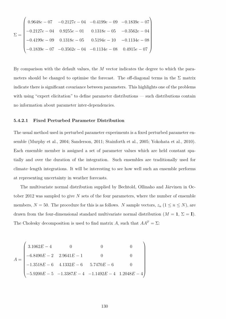
Σ =
0.9648e− 07 −0.2127e− 04 −0.4199e− 09 −0.1839e− 07
−0.2127e− 04 0.9255e− 01 0.1318e− 05 −0.3562e− 04
−0.4199e− 09 0.1318e− 05 0.5194e− 10 −0.1134e− 08
−0.1839e− 07 −0.3562e− 04 −0.1134e− 08 0.4915e− 07
By comparison with the default values, the M vector indicates the degree to which the para-
meters should be changed to optimise the forecast. The off-diagonal terms in the Σ matrix
indicate there is significant covariance between parameters. This highlights one of the problems
with using “expert elicitation” to define parameter distributions — such distributions contain
no information about parameter inter-dependencies.
5.4.2.1 Fixed Perturbed Parameter Distribution
The usual method used in perturbed parameter experiments is a fixed perturbed parameter en-
semble (Murphy et al., 2004; Sanderson, 2011; Stainforth et al., 2005; Yokohata et al., 2010).
Each ensemble member is assigned a set of parameter values which are held constant spa-
tially and over the duration of the integration. Such ensembles are traditionally used for
climate–length integrations. It will be interesting to see how well such an ensemble performs
at representing uncertainty in weather forecasts.
The multivariate normal distribution supplied by Bechtold, Ollinaho and Jarvinen in Oc-
tober 2012 was sampled to give N sets of the four parameters, where the number of ensemble
members, N = 50. The procedure for this is as follows. N sample vectors, zn (1 ≤ n ≤ N), are
drawn from the four-dimensional standard multivariate normal distribution (M = 1, Σ = I).
The Cholesky decomposition is used to find matrix A, such that AAT = Σ:
A =
3.1062E − 4 0 0 0
−6.8490E − 2 2.9641E − 1 0 0
−1.3518E − 6 4.1332E − 6 5.7470E − 6 0
−5.9200E − 5 −1.3387E − 4 −1.1492E − 4 1.2048E − 4
130

The samples from the standard multivariate distribution are transformed to samples from the
correct parameter distribution, xn, using the transformation:
xn = M + Azn (5.3)
Two types of fixed perturbed parameter ensemble are considered here. The first uses the
same fifty sets of four parameters for all starting dates (“TSCP”). Sampling of the parameters
is performed offline: Latin hypercube sampling is used to define fifty percentiles at which
to sample the standard multivariate normal distribution, before (5.3) is used to transform to
parameter space. This technique ensures the joint distribution is fully explored. The covariance
of the resultant sample is checked against the EPPES covariance matrix; 10,000 iterations found
a sample whose covariance matrix differed by less than 5% from the true matrix. The sampled
parameter values are shown in Table 5.2. The second type of fixed perturbed parameter
ensemble uses N new sets of parameters for each initial condition (“TSCPr”). This sampling
is performed online, and the samples are not optimised. However, when forecasts from many
starting conditions are taken together, the ensemble is sufficient to fully sample the joint pdf.
5.4.2.2 Stochastically Varying Perturbed Parameter Distribution
Khouider and Majda (2006) recognise that a problem with many deterministic parametrisation
schemes is the presence of parameters that are “nonphysically kept fixed/constant and spatially
homogeneous”. An alternative to the fixed perturbed parameter ensemble described above is a
stochastically varying perturbed parameter ensemble (“TSCPv”) where the parameter values
are varied spatially and temporally following the EPPES distribution. However, the EPPES
technique contains no information about the correct spatial and temporal scales on which to
vary the parameters. Since the likelihood function is evaluated at day ten of the forecast, the
set of parameters must perform well over this time window to produce a skilful forecast; this
indicates that ten days could be a suitable temporal scale. The likelihood function evaluates
the skill of the forecast using the geopotential height at 500 hPa. The likelihood function
will therefore focus on the midlatitudes, where the geopotential height has high variability. A
suitable spatial scale could therefore be ∼ 1000 km. The SPPT spectral pattern generator is
a suitable technique for stochastically varying the parameters in the convection scheme. It
generates a spatially and temporally correlated field of random numbers.
131
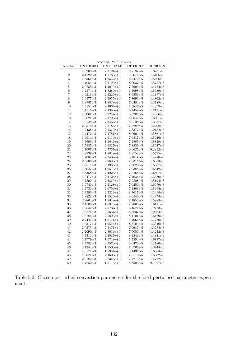
Selected PermutationsNumber ENTRORG ENTSHALP DETRPEN RPRCON
1 1.8203e-3 2.3121e+0 8.7197e-5 1.3731e-32 2.4122e-3 1.7785e+0 6.8076e-5 1.5406e-33 1.6561e-3 1.9652e+0 6.8473e-5 1.6606e-34 1.1054e-3 2.4199e+0 8.0037e-5 1.5757e-35 2.0785e-3 1.4016e+0 7.5603e-5 1.4454e-36 1.7574e-3 1.8280e+0 6.4998e-5 1.6689e-37 1.9311e-3 2.2220e+0 8.9559e-5 1.1177e-38 1.6377e-3 2.4955e+0 7.8693e-5 1.4802e-39 1.8987e-3 1.9838e+0 7.6484e-5 1.3189e-310 1.5554e-3 2.4064e+0 7.5846e-5 1.4879e-311 1.4116e-3 2.1398e+0 6.7459e-5 1.7171e-312 1.5061e-3 2.2247e+0 8.3208e-5 1.4336e-313 1.9821e-3 2.3726e+0 8.0642e-5 1.3901e-314 1.9148e-3 2.3462e+0 8.5138e-5 1.3017e-315 2.0575e-3 2.3785e+0 7.5289e-5 1.4298e-316 1.2438e-3 2.2379e+0 7.3377e-5 1.9182e-317 1.4471e-3 2.1781e+0 8.0664e-5 1.5861e-318 1.6914e-3 2.6139e+0 7.6817e-5 1.5926e-319 1.3696e-3 1.9646e+0 7.4865e-5 1.8839e-320 1.5985e-3 2.0827e+0 7.8839e-5 1.8027e-321 2.1007e-3 2.7757e+0 9.9625e-5 9.2852e-422 1.9999e-3 1.8012e+0 7.8752e-5 1.5595e-323 1.7084e-3 2.2402e+0 8.1817e-5 1.4210e-324 2.5506e-3 2.0698e+0 7.2315e-5 1.6063e-325 1.8514e-3 2.1935e+0 7.3820e-5 1.6587e-326 1.8047e-3 1.9516e+0 7.9388e-5 1.6842e-327 1.8358e-3 2.1223e+0 7.5268e-5 1.6807e-328 1.9477e-3 2.1125e+0 7.7636e-5 1.3370e-329 1.7890e-3 2.3366e+0 7.9808e-5 1.5194e-330 1.6740e-3 2.1128e+0 7.6250e-5 1.6079e-331 1.7733e-3 2.0756e+0 7.1866e-5 1.8394e-332 2.3390e-3 2.5212e+0 8.4617e-5 1.1419e-333 1.8828e-3 1.9526e+0 8.0540e-5 1.4474e-334 2.2864e-3 1.8812e+0 7.4853e-5 1.5983e-335 2.1500e-3 1.5878e+0 7.2808e-5 1.6111e-336 1.9647e-3 2.6737e+0 8.4574e-5 1.2773e-337 1.5776e-3 2.5651e+0 8.6837e-5 1.2864e-338 1.6185e-3 2.5899e+0 8.1101e-5 1.3479e-339 2.2445e-3 1.6171e+0 6.7066e-5 1.7770e-340 1.5317e-3 1.9515e+0 8.3194e-5 1.3346e-341 2.0375e-3 2.2471e+0 7.9687e-5 1.3254e-342 2.2090e-3 2.3014e+0 7.0050e-5 1.4242e-343 1.7413e-3 2.2027e+0 8.2246e-5 1.4821e-344 2.1779e-3 1.6718e+0 5.7394e-5 1.6127e-345 1.4782e-3 2.5573e+0 9.0479e-5 1.2180e-346 2.1244e-3 1.9506e+0 7.9765e-5 1.3744e-347 1.3171e-3 1.8954e+0 8.4434e-5 1.6384e-348 1.8671e-3 2.1600e+0 7.8113e-5 1.5982e-349 2.0184e-3 2.2348e+0 7.7212e-5 1.4772e-350 1.7250e-3 1.6116e+0 6.8595e-5 2.1027e-3
Table 5.2: Chosen perturbed convection parameters for the fixed perturbed parameter experi-ment.
132

In this experiment the standard SPPT settings were used in the pattern generator. A three
scale composite pattern is used which has the same spatial and temporal correlations as used
in SPPT. The standard deviations of these independent patterns are 0.939 (smallest scale),
0.325 and 0.108 (largest scale) to give a total standard deviation of 1. These settings vary the
parameters faster and on smaller spatial scales than the scales to which EPPES is sensitive,
as estimated above. However it will still be useful as a first test, and when combined with
the fixed perturbed parameter ensemble (varying on an ∞ spatial and temporal scale), it can
provide bounds on the skill of such a representation of model uncertainty.
The SPPT pattern generator is used to generate four independent composite fields with
mean 0 and standard deviation 1. The correct covariance structure is introduced using the
transformation matrix, A: xi,j,t = M + Azi,j,t, where the indices i, j refer to latitude and
longitude and t refers to time. The parameters do not vary as a function of height since the
convection parametrisation is applied columnwise in the model. The resultant four covarying
fields are used to define the values of the four convection parameters as a function of position
and time.
5.5 Experimental Procedure
Parameter estimation was carried out with the EPPES system using IFS model version CY37R3
for 45 dates between 12 May 2011 and 8 August 2011, with forecasts initialised every 48
hours. The same model version is used here for consistency. Different initial dates to those
used to estimate the joint pdfs must be selected (an out of sample test), but taken from the
same time of the year since the EPPES estimated pdfs may be seasonally dependent. In
order to detect improvements in the model uncertainty representation, it is important that
initial condition uncertainty is well represented in the ensemble forecast. The best technique
possible will be used, which for the IFS involves using hybrid EDA/singular vector estimates
for the perturbations. The initial dates used must be after June 2010, when the EDA system
became operational. The selected dates for the hindcasts are therefore from Summer 2012.
The parametrisation schemes will be tested at T159 (1.125◦) using a fifty member ensemble
forecast. The schemes are tested using ten-day hindcasts initialised every five days between
14 April and 6 September 2012 (30 dates in total). Persistent SSTs are used instead of a
dynamical ocean. The high-resolution ECMWF 4DVar analysis is used for verification.
133

Other Four Tendencies: SPPTConvection: Zero TSCZConvection: SPPT TSCSConvection: Perturbed Parameters (constant) TSCPConvection: Perturbed Parameters (resampled) TSCPrConvection: Perturbed Parameters (varying) TSCPv
Table 5.3: Proposed experiments for investigating the representation of uncertainty in theECMWF convection parametrisation scheme.
Five experiments are proposed to investigate the representation of model uncertainty in
the convection scheme in the IFS (Table 5.3). In each experiment, the uncertainty in the other
four parametrisation tendencies (radiation, turbulence and gravity wave drag, non-orographic
gravity wave drag, large scale water processes) is represented by SPPT (“TS”). In the first
experiment, there is no representation of uncertainty in the convection tendency (“CZ”). In
the second, SPPT is used to represent uncertainty in the convection tendency (“CS” — equi-
valent to the operational SPPT parametrisation scheme). In the final three, uncertainty in
the convection tendency is represented by a static perturbed parameter ensemble, with and
without resampling of parameters for different start dates (“CPr” and “CP” respectively), and
by a stochastically varying perturbed parameter ensemble (“CPv”).
In order to compare the different representations of convection model uncertainty, the SPPT
scheme must correctly account for uncertainty in the other four tendencies. Therefore verific-
ation will be performed in a two stage process. Firstly, the calibration of the ensemble will
be checked in a region with little uncertainty due to convection, i.e., where there is little con-
vective activity. The five experiments in Table 5.3 should perform very similarly in this region
as they have the same representation of uncertainty in the other four tendencies. Secondly,
a region where convection is the dominant process will be selected to test the different un-
certainty schemes. Given that model uncertainty has been accounted for in the other four
parametrisations using SPPT, and that a region has been selected where the model uncer-
tainty is dominated by deep convection, a scheme which accurately represents uncertainty in
deep convection will give a reliable forecast in this region, and any detected improvements
in forecast skill can be attributed to an improvement in representation of uncertainty in the
convection scheme.
134

0 30 60 90 120 150 180 210 240 270 300 330 360−90
−60
−30
0
30
60
90
longitude / o E
latit
ude
/ o N
(a)
0 30 60 90 120 150 180 210 240 270 300 330 360−90
−60
−30
0
30
60
90
longitude / o E
latit
ude
/ o N
(b)
0
0.1
0.2
0.3
0.4
0.5
0.6
Figure 5.1: Convection diagnostic (colour) derived from the IFS tendencies calculated as partof the YOTC project (see text for details). (a) Regions where the diagnostic is close to zero(bounded by grey boxes), indicating there is little convection. (b) Regions where the diagnosticis large (bounded by grey box), indicating convection is the dominant process.
5.5.1 Definition of Verification Regions
The regions of interest are defined using the Year of Tropical Convection (YOTC) dataset from
ECMWF. YOTC was a joint WCRP and World Weather Research Programme/The Observing-
System Research and Predictability Experiment (WWRP/THORPEX) project which aimed
to focus research efforts on the problem of organised tropical convection. The ECMWF YOTC
dataset consists of high resolution analysis and forecast data for May 2008 — April 2010. In
particular, the IFS parametrisation tendencies were archived at every time step out to a lead
time of ten days.
The 24-hour cumulative temperature tendencies at 850 hPa for each parametrisation scheme
are used. Forecasts initialised from 30 dates between 14 April and 6 September 2009 are selec-
ted, with subsequent start dates separated by five days. To identify regions where convection is
the dominant process, the ratio between the magnitude of the convective tendency and the sum
of the magnitudes of all tendencies is calculated, and is shown in Figure 5.1. This diagnostic
135

can be used to define regions where there is little convection (the ratio is close to zero) or
where convection dominates (the ratio greater than 0.5). Since the forecasting skill of the IFS
is strongly latitudinally dependent, both the regions with little convection and with significant
convection are defined in the tropics (25◦S–25◦N). Both regions are approximately the same
size, and cover areas of both land and sea. Any differences in the forecast verification between
these two regions will be predominantly due to convection.
5.5.2 Chosen Diagnostics
Four variables of interest have been selected which will be used to verify the forecasts. Tem-
perature and zonal wind at 850 hPa (T850 and U850 respectively), correspond to fields at
approximately 1.5 km altitude, and falls above the boundary layer in many places. The geopo-
tential height at 500 hPa (Z500) is a standard ECMWF diagnostic variable. It is particularly
useful in the extra-tropics where it shows characteristic features corresponding to low and high
pressure weather systems. The zonal wind at 200 hPa (U200) is particularly interesting when
considering convection. This is because 200 hPa falls close to the tropopause, where deep
convection is capped. Convective outflow often occurs at this level, which can be detected in
U200.
For each variable, the impact of the schemes will be evaluated using a number of the
diagnostics described in Chapter 1:
• Bias (Section 1.7.2.1)
• RMSE compared to RMS spread (Section 1.7.3.1)
• RMS error-spread graphical diagnostic (Section 1.7.3.1)
• Forecast skill scores: RPSS, IGNSS, ESS (Sections 1.7.1.2 and 1.7.1.3, and Chapter 4
respectively)
In convecting regions, precipitation (PPT) and total column water vapour (TCWV) will also
be considered. PPT is a parametrised product of the convection and large scale water processes
parametrisation schemes, so an improvement to the convection scheme should be detectable by
studying this variable. The convection scheme effectively redistributes and removes moisture
from the atmosphere, so an improvement in TCWV could be indicative of an improvement in
the convection scheme.
136

0 50 100 150 200
−0.3
−0.25
−0.2
−0.15
−0.1
−0.05
0
0.05
lead time / hrs
% B
ias
(a)(a)(a)(a)(a) T 850
0 50 100 150 200
−2
0
2
4
6
8
10
lead time / hrs
% B
ias
(b)(b)(b)(b)(b) U 850
0 50 100 150 200−0.2
−0.15
−0.1
−0.05
0
0.05
lead time / hrs
% B
ias
(c)(c)(c)(c)(c) Z 500
0 50 100 150 200
−10
−8
−6
−4
−2
0
2
lead time / hrs
% B
ias
(d)(d)(d)(d)(d) U 200
Figure 5.2: Percentage forecast bias in tropical regions with little convection as a function oftime for (a) T850, (b) U850, (c) Z500 and (d) U200. Results are shown for the five experiments:black — TSCZ; blue — TSCS; red — TSCP; magenta — TSCPr; green — TSCPv. The biasis calculated as described in the text, and given as a percentage of the root mean square of theanalysis in the region of interest. The red line is obscured by the magenta line in each figure.
5.6 Verification of Forecasts
5.6.1 Verification in Non-Convecting Regions
Firstly, the impact of the different representations of model uncertainty will be considered in
the non-convecting regions defined in Figure 5.1(a). Figure 5.2 shows the percentage bias of
forecasts, calculated following (1.24), for regions of little convection. This is a useful diagnostic,
as it can indicate the presence of systematic errors in a forecast. A small change is observed
in the bias when different uncertainty schemes are used, and in particular the TSCPv scheme
(green) performs well for all variables considered. As expected, the TSCP and TSCPr schemes
(red and magenta respectively) perform similarly — the bias in the ensemble mean is unaffected
by whether the parameter perturbations are resampled for each initial condition. For U850,
Z500 and U200, the TSCZ scheme (black) outperforms the TSCS scheme (blue), a result which
will be discussed in Section 5.7.
The impact of the uncertainty schemes on the calibration of the ensemble can be summarised
by evaluating the RMS error in the ensemble mean and the RMS ensemble spread as a function
of time within the region of interest, which should be equal for a well calibrated ensemble.
137

0 50 100 150 200
1
1.5
2
lead time / hrs
RM
S
(a) T 850
0 50 100 150 200
1.5
2
2.5
3
3.5
lead time / hrs
RM
S
(b) U 850
0 50 100 150 20020
40
60
80
100
120
140
160
lead time / hrs
RM
S
(c) Z 500
0 50 100 150 200
2
3
4
5
6
7
8
lead time / hrs
RM
S
(d) U 200
Figure 5.3: Temporal evolution of root mean square ensemble spread (dashed lines) and rootmean square error (solid lines) for regions with little convection for (a) T850, (b) U850, (c)Z500 and (d) U200. Results are shown for the five experiments: black — TSCZ; blue — TSCS;red — TSCP; magenta — TSCPr; green — TSCPv. The grey curves indicate the results forthe operational (T639) EPS forecasts for comparison. The red line is obscured by the magentaline in each figure.
Figure 5.3 shows this diagnostic for the regions with little convection. Forecasts are observed
to be slightly under-dispersive for all variables. The underdispersion is large for Z500, but is
small for the other variables (note that the y-axes do not start at zero). For comparison, the
RMS spread and error curves are also shown for operational ensemble forecasts at T639 (grey).
At this higher resolution the ensemble spread is similar, but the RMSE is smaller. The low
resolution (T159) used in the five test experiments is responsible for the higher RMSE and
therefore contributes to the under-dispersive nature of the ensemble.
A more comprehensive understanding of the calibration of the ensemble can be gained by
considering the RMS error-spread diagnostic. The forecast-verification pairs are collected for
each spatial point in the region of interest for each starting condition. These pairs are ordered
according to their forecast variance, and divided into 30 equally populated bins. The RMS
spread and RMSE are evaluated for each bin and displayed on scatter plots. Figure 5.4 shows
this diagnostic for regions with little convection at lead times of one, three and ten days.
The scattered points should lie on the one-to-one diagonal, shown in black, for a statistically
consistent ensemble following (1.26). The diagnostic indicates a large degree of flow-dependent
spread in the ensemble forecasts, with scattered points lying close to the one-to-one line. The
138

T850 forecasts are particularly well calibrated, and the spread of the U850 and U200 forecasts
are also a skilful indicator of the expected error for all five experiments. The Z500 forecasts
show little flow dependency at short lead times, but improve when the longer ten-day forecasts
are considered. As expected, the results from the five experiments are very similar, and show
moderately under-dispersive but otherwise well calibrated forecasts.
5.6.2 Verification in Convecting Regions
The previous section indicates that the model uncertainty in the other four tendencies is suffi-
ciently well represented by SPPT. This section considers forecasts for the strongly convecting
regions defined in Figure 5.1(b) to evaluate the impact of the new uncertainty schemes. Fig-
ure 5.5 shows the percentage bias for forecasts of T850, U850, Z500 and U200 in this region
for the five different schemes considered. The bias is similar for all schemes; no one scheme is
systematically better or worse than the others.
Figure 5.6 shows the RMS error and spread as a function of time averaged over all cases
for all points within the region of interest. The RMS error in the forecast is similar for all
experiments — the perturbed parameter ensembles have not resulted in an increase in error
over the operational scheme, except for a slight increase for T850. However, the fixed perturbed
parameter ensemble (red/magenta) has resulted in an increase in spread over the operational
TSCS forecast (blue). This is especially large for T850, where the observed increase is 25%
at long lead times. Interestingly, the TSCZ ‘deterministic convection’ forecasts of T850 also
result in an increase in ensemble spread over TSCS. This is a counter-intuitive result, as it is
expected that using a stochastic parametrisation would increase the spread of the ensemble.
This result will be discussed in Section 5.7, and motivates the experiments carried out in
Chapter 6. For comparison, the results for the operational EPS are also shown in grey. As
is the case in regions with little convection, some of the ensemble under-dispersion at T159 is
due to an increased forecast RMSE compared to the operational T639 forecasts, though the
forecasts are under-dispersive at both resolutions.
Figure 5.7 shows the RMS error-spread graphical diagnostic for the five forecast models in
regions with significant convection. The impact of the different schemes is slight. However,
there is a larger difference than in regions with little convection (see Figure 5.4). All schemes
remain well calibrated, and do not show large increases in error compared to the operational
139

0 1 20
0.5
1
1.5
2
2.5
Forecast Spread
RM
SE
(a)
0 1 2 30
1
2
3
Forecast SpreadR
MS
E
(b)
0 2 40
1
2
3
4
Forecast Spread
RM
SE
(c)
0 1 20
0.5
1
1.5
2
2.5
Forecast Spread
RM
SE
(d)
0 1 2 30
1
2
3
4
Forecast Spread
RM
SE
(e)
0 2 40
1
2
3
4
5
Forecast SpreadR
MS
E
(f)
0 20 400
20
40
60
Forecast Spread
RM
SE
(g)
0 20 40 60 800
50
100
Forecast Spread
RM
SE
(h)
0 100 2000
100
200
300
Forecast Spread
RM
SE
(i)
0 2 40
1
2
3
4
Forecast Spread
RM
SE
(j)
0 2 4 60
2
4
6
8
Forecast Spread
RM
SE
(k)
0 5 100
2
4
6
8
10
Forecast Spread
RM
SE
(l)
Figure 5.4: Root mean square error-spread diagnostic for tropical regions with little convec-tion for (a)–(c) T850, (d)–(f) U850, (g)–(i) Z500 and (j)–(l) U200, at lead times of 1 day (firstcolumn), 3 days (second column) and 10 days (third column) for each variable. Results areshown for the five experiments: black — TSCZ; blue — TSCS; red — TSCP; magenta —TSCPr; green — TSCPv. For a well calibrated ensemble, the scattered points should lie onthe one-to-one diagonal shown in black.
140

0 50 100 150 200−0.2
−0.15
−0.1
−0.05
0
0.05
lead time / hrs
% B
ias
T 850(a)(a)(a)(a)(a)
0 50 100 150 200−20
−15
−10
−5
0
lead time / hrs
% B
ias
U 850(b)(b)(b)(b)(b)
0 50 100 150 200−0.25
−0.2
−0.15
−0.1
−0.05
0
lead time / hrs
% B
ias
Z 500(c)(c)(c)(c)(c)
0 50 100 150 2000
5
10
15
20
lead time / hrs
% B
ias
U 200(d)(d)(d)(d)(d)
Figure 5.5: Percentage forecast bias in tropical regions with significant convection as afunction of time for (a) T850, (b) U850, (c) Z500 and (d) U200. Results are shown for thefive experiments: black — TSCZ; blue — TSCS; red — TSCP; magenta — TSCPr; green —TSCPv. The bias is calculated as described in the text, and given as a percentage of the rootmean square of the analysis in the region of interest. The red line is obscured by the magentaline in each figure.
0 50 100 150 2000.3
0.4
0.5
0.6
0.7
0.8
0.9
lead time / hrs
RM
S
(a) T 850
0 50 100 150 200
1
1.5
2
2.5
3
3.5
lead time / hrs
RM
S
(b) U 850
0 50 100 150 200
50
100
150
lead time / hrs
RM
S
(c) Z 500
0 50 100 150 200
2
3
4
5
6
7
lead time / hrs
RM
S
(d) U 200
Figure 5.6: Temporal evolution of root mean square ensemble spread (dashed lines) and rootmean square error (solid lines) for regions with significant convection for (a) T850, (b)U850, (c) Z500 and (d) U200. Results are shown for the five experiments: black — TSCZ;blue — TSCS; red — TSCP; magenta — TSCPr; green — TSCPv. The grey curves indicatethe results for the operational (T639) EPS forecasts for comparison. The red line is obscuredby the magenta line in each figure.
141

TSCS forecasts. The fixed perturbed parameter schemes (red and magenta) have larger spread
than the other schemes, which is most apparent for T850 in Figures 5.7(a–c). TSCS (blue)
has the most under-dispersive ensemble at long lead times, though is better calibrated than
the other experiments at short lead times. The TSCPv experiment has intermediate spread,
improving on TSCS but under-dispersive compared to the TSCP experiments.
The skill of the forecasts is evaluated using the RPS, IGN and ES as a function of lead
time, and the skill scores evaluated with respect to the climatological forecast for the con-
vecting region. The results are shown in Figure 5.8 for each variable of interest. There is
no significant difference between the TSCP and TSCPr forecasts according to the skill scores.
The TSCP/TSCPr schemes score highly for a range of variables according to each score: they
perform significantly better than the other forecasts for T850 according to RPSS and IGNSS,
for U850 according to IGNSS and ESS, and for Z500 according to all scores (see Appendix A
for details of significance testing). For U200, the TSCS forecasts are significantly better than
the other forecasts, and the TSCZ forecasts are significantly poorer. However for the other
variables, TSCS performs comparatively poorly, and often produces significantly the worst
forecasts. This is probably due to the poorer forecast ensemble spread.
5.6.2.1 Precipitation Forecasts
The impact of the different model uncertainty schemes on forecasts of convective precipitation
is a good indicator of improvement in the convection scheme. However, it is difficult to verify
precipitation forecasts as measurements of precipitation are not assimilated into the IFS using
the 4DVar or EDA systems, unlike T, U and Z. One option is to use short-range high resolution
(T1279) deterministic forecasts for verification. However, there are known problems with spin-
up for accumulated fields like precipitation — the model takes a few time steps to adjust to
the initial conditions (Kaallberg, 2011). Instead, the Global Precipitation Climatology Project
(GPCP) dataset is used for verification of precipitation forecasts. The GPCP, established by
the WCRP, combines information from a large number of satellite and ground based sources
to estimate the global distribution of precipitation. The data set used here is the One-Degree
Daily (1DD) product (Huffman et al., 2001), which has been conservatively re-gridded onto a
T159 reduced Gaussian grid to allow comparison with the IFS forecasts.
Figure 5.9 shows the RMS error-spread diagnostic for convective precipitation. All forecasts
142

0.2 0.4 0.6 0.8 1 1.2
0.2
0.4
0.6
0.8
1
1.2
Forecast Spread
RM
SE
(a)
0.2 0.4 0.6 0.8 1 1.2 1.4
0.5
1
1.5
Forecast Spread
RM
SE
(b)
0.5 1 1.5
0.5
1
1.5
2
Forecast Spread
RM
SE
(c)
0.5 1 1.5 2 2.50.5
1
1.5
2
2.5
3
Forecast Spread
RM
SE
(d)
1 2 3
1
2
3
4
Forecast Spread
RM
SE
(e)
1 2 3 4 51
2
3
4
5
6
Forecast Spread
RM
SE
(f)
20 40 60
20
40
60
80
Forecast Spread
RM
SE
(g)
20 40 60 80 100
50
100
150
200
Forecast Spread
RM
SE
(h)
50 100 150
50
100
150
200
250
Forecast Spread
RM
SE
(i)
1 2 3 4 51
2
3
4
5
Forecast Spread
RM
SE
(j)
2 4 6
2
3
4
5
6
Forecast Spread
RM
SE
(k)
2 4 6 8 102
4
6
8
10
Forecast Spread
RM
SE
(l)
Figure 5.7: Root mean square error-spread diagnostic for tropical regions with significantconvection for (a)–(c) T850, (d)–(f) U850, (g)–(i) Z500 and (j)–(l) U200, at lead times of1 day (first column), 3 days (second column) and 10 days (third column) for each variable.Results are shown for the five experiments: black — TSCZ; blue — TSCS; red — TSCP;magenta — TSCPr; green — TSCPv. For a well calibrated ensemble, the scattered pointsshould lie on the one-to-one diagonal shown in black.
143
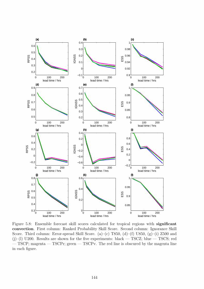
0 100 200
0.2
0.3
0.4
0.5
0.6
lead time / hrs
RP
SS
(a)(a)(a)(a)(a)
0 100 200−0.1
0
0.1
0.2
0.3
0.4
lead time / hrs
IGN
SS
(b)(b)(b)(b)(b)
0 100 2000.9
0.92
0.94
0.96
0.98
1
lead time / hrs
ES
S
(c)(c)(c)(c)(c)
0 100 200
0.5
0.6
0.7
0.8
0.9
lead time / hrs
RP
SS
(d)(d)(d)(d)(d)
0 100 200
0.2
0.3
0.4
0.5
0.6
0.7
lead time / hrs
IGN
SS
(e)(e)(e)(e)(e)
0 100 200
0.8
0.85
0.9
0.95
1
lead time / hrsE
SS
(f)(f)(f)(f)(f)
0 100 200
−0.2
0
0.2
0.4
0.6
lead time / hrs
RP
SS
(g)(g)(g)(g)(g)
0 100 200
−0.6
−0.4
−0.2
0
0.2
0.4
lead time / hrs
IGN
SS
(h)(h)(h)(h)(h)
0 100 200−0.2
0
0.2
0.4
0.6
0.8
lead time / hrs
ES
S
(i)(i)(i)(i)(i)
0 100 2000.3
0.4
0.5
0.6
0.7
0.8
lead time / hrs
RP
SS
(j)(j)(j)(j)(j)
0 100 2000
0.2
0.4
0.6
lead time / hrs
IGN
SS
(k)(k)(k)(k)(k)
0 100 200
0.85
0.9
0.95
1
lead time / hrs
ES
S
(l)(l)(l)(l)(l)
Figure 5.8: Ensemble forecast skill scores calculated for tropical regions with significantconvection. First column: Ranked Probability Skill Score. Second column: Ignorance SkillScore. Third column: Error-spread Skill Score. (a)–(c) T850, (d)–(f) U850, (g)–(i) Z500 and(j)–(l) U200. Results are shown for the five experiments: black — TSCZ; blue — TSCS; red— TSCP; magenta — TSCPr; green — TSCPv. The red line is obscured by the magenta linein each figure.
144

0 0.005 0.010
0.005
0.01
0.015
Forecast Spread
RM
SE
(a)
0 0.005 0.010
0.005
0.01
0.015
Forecast Spread
RM
SE
(b)
0 0.005 0.01 0.0150
0.005
0.01
0.015
Forecast Spread
RM
SE
(c)
Figure 5.9: RMS error-spread diagnostic for cumulative convective precipitation for the 24 hourwindow before a lead time of (a) 1 day, (b) 3 days and (c) 10 days. The diagnostic is calculatedfor tropical regions with significant convection. Results are shown for the five experiments:black — TSCZ; blue — TSCS; red — TSCP; magenta — TSCPr; green — TSCPv. For a wellcalibrated ensemble, the scattered points should lie on the one-to-one diagonal shown in black.
are under-dispersive, and the different uncertainty schemes have only a slight impact on the
calibration of the ensemble. Figure 5.10(b) indicates more clearly the impact of the different
schemes on the ensemble spread and error. On average, the TSCZ scheme is significantly the
most under-dispersive and has a significantly larger RMSE. The two stochastic schemes, TSCS
and TSCPv, have significantly the smallest error. TSCS has significantly the largest spread at
short lead times, and TSCP and TSCPr have significantly the largest spread at later lead times.
Figure 5.10(a) shows the bias in forecasts of convective precipitation. The stochastic schemes,
TSCS and TSCPv, have the smallest bias over the entire forecasting window. Figures 5.10(c)–
(e) show the forecast skill scores for convective precipitation. TSCS is significantly the best
between days three and five according to RPS and ES. TSCZ is significantly the poorest
according to RPS, but the other schemes score very similarly. ES and IGN also score TSCZ as
significantly the worst at early lead times, but at later lead times, no one scheme is significantly
different to the others.
It is important for a model to capture the spatial and temporal characteristics of precip-
itation. The global frequency distribution of rain rate (in mm/day) was considered for the
different forecast models and compared to the GPCP 1DD dataset. The results are shown
in Figure 5.11. All five forecast models perform similarly well, and no one model performs
particularly well or poorly compared to the others. All forecasts under-predict the proportion
of low rain rates and over predict the proportion of high rain rates when compared to the
GPCP data set (grey), but overall predict the distribution of rain rates well.
The spatial distribution of cumulative precipitation (convective plus large scale) was also
145
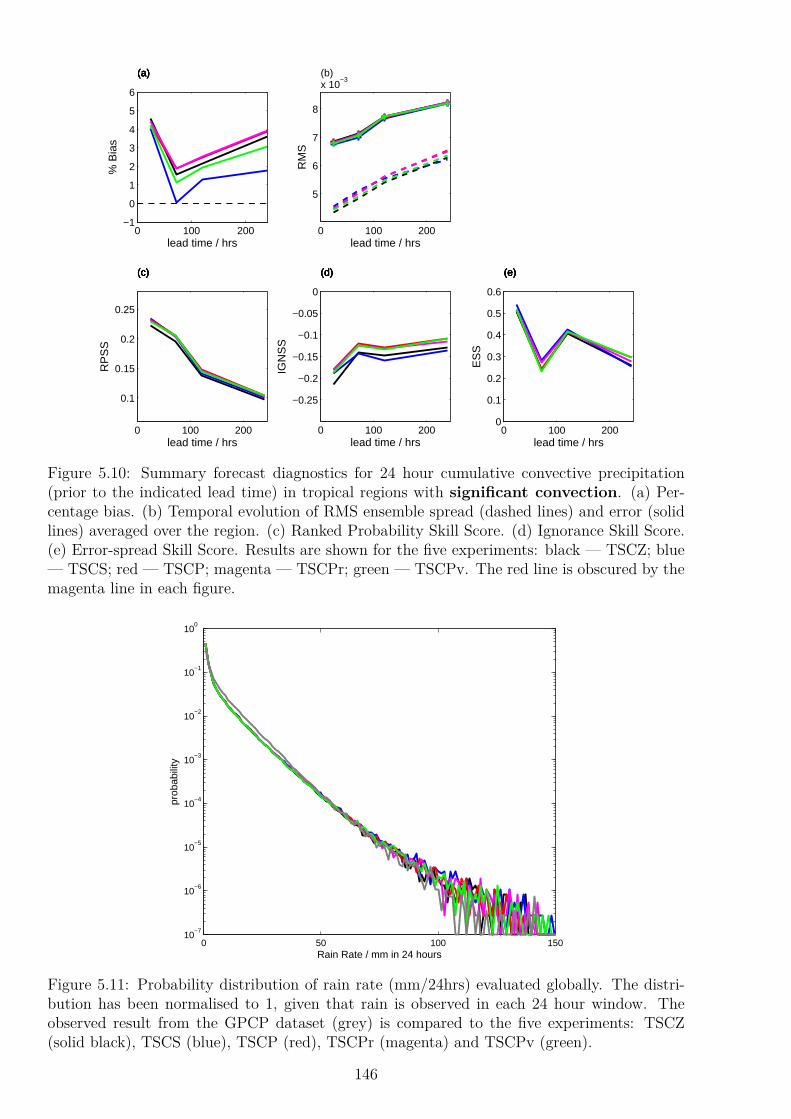
0 100 200−1
0
1
2
3
4
5
6
lead time / hrs
% B
ias
(a)(a)(a)(a)(a)
0 100 200
5
6
7
8
x 10−3
lead time / hrs
RM
S
(b)
0 100 200
0.1
0.15
0.2
0.25
lead time / hrs
RP
SS
(c)(c)(c)(c)(c)
0 100 200
−0.25
−0.2
−0.15
−0.1
−0.05
0
lead time / hrs
IGN
SS
(d)(d)(d)(d)(d)
0 100 2000
0.1
0.2
0.3
0.4
0.5
0.6
lead time / hrs
ES
S
(e)(e)(e)(e)(e)
Figure 5.10: Summary forecast diagnostics for 24 hour cumulative convective precipitation(prior to the indicated lead time) in tropical regions with significant convection. (a) Per-centage bias. (b) Temporal evolution of RMS ensemble spread (dashed lines) and error (solidlines) averaged over the region. (c) Ranked Probability Skill Score. (d) Ignorance Skill Score.(e) Error-spread Skill Score. Results are shown for the five experiments: black — TSCZ; blue— TSCS; red — TSCP; magenta — TSCPr; green — TSCPv. The red line is obscured by themagenta line in each figure.
0 50 100 15010
−7
10−6
10−5
10−4
10−3
10−2
10−1
100
Rain Rate / mm in 24 hours
prob
abili
ty
Figure 5.11: Probability distribution of rain rate (mm/24hrs) evaluated globally. The distri-bution has been normalised to 1, given that rain is observed in each 24 hour window. Theobserved result from the GPCP dataset (grey) is compared to the five experiments: TSCZ(solid black), TSCS (blue), TSCP (red), TSCPr (magenta) and TSCPv (green).
146

considered for the different forecast models. All schemes performed equally well (not shown).
When compared to the GPCP data, all showed too much precipitation over the ocean, and in
particular forecast intensities of rain in the intertropical and South Pacific convergence zones
that were higher than observed. The results were indistinguishable by eye — the difference
between forecast and observations is far greater than the differences between different forecasts.
5.6.2.2 Total Column Water Vapour
The impact of the different model uncertainty schemes on forecasts of total column water
vapour (TCWV) is also a good indicator of improvement in the convection scheme. Figure 5.12
shows the RMS error-spread diagnostic for TCWV. The forecasts for this variable are poorly
calibrated when compared to convective precipitation. The RMSE is systematically larger
than the spread, and the slope of the scattered points is too shallow. This shallow slope
indicates that the forecasting system is unable to distinguish between cases with low and high
predictability for this variable — the expected error in the ensemble mean is poorly predicted
by the ensemble spread. The different forecast schemes show a larger impact than for forecasts
of precipitation — the TSCS model produces forecasts which are under-dispersive compared
to the other forecasts. Figure 5.13 shows (a) the bias, (b) the RMSE and spread as a function
of time, and (c)–(e) the forecast skill scores for each experiment. Figure (b) shows that the
TSCPv forecasts have significantly the largest spread at lead times of 24 hours and greater. The
TSCS forecasts have significantly the smallest spread at later lead times, but also significantly
the largest error at all lead times. Figure 5.13 (a) shows the bias is also largest for the TSCS
forecasts, and Figure 5.13 (c–e) indicates the skill is the lowest.
An early version of SPPT was found to dry out the tropics, and resulted in a decrease in
TCWV of approximately 10% (Martin Leutbecher, pers. comm., 2013). This was corrected in a
later version. It is possible that TCWV could be sensitive to the proposed perturbed parameter
representations of model uncertainty. The average TCWV between 20◦N and 20◦S is averaged
over all start dates separately for each ensemble member, and is shown in Figure 5.14. Initially,
all experiments show a drying of the tropics of approximately 0.5 kgm−2 over the first 12 hours,
indicating a spin-up period in the model. The TSCZ, TSCS and TSCPv forecasts then stabilise.
However, each ensemble member in the TSCP model has vastly different behaviour, with some
showing systematic drying, and others showing systematic moistening over the ten day forecast.
147

1 2 3 4 5
1
2
3
4
5
Forecast Spread
RM
SE
(a)
(a)
2 4 6
1
2
3
4
5
6
7
Forecast SpreadR
MS
E(b)
(b)
2 4 6 8
2
4
6
8
Forecast Spread
RM
SE
(c)
(c)
Figure 5.12: RMS error-spread diagnostic for total column water vapour for lead times of(a) 1 day, (b) 3 days and (c) 10 days. The diagnostic is calculated for tropical regions withsignificant convection. Results are shown for the five experiments: black — TSCZ; blue —TSCS; red — TSCP; magenta — TSCPr; green — TSCPv. For a well calibrated ensemble,the scattered points should lie on the one-to-one diagonal shown in black.
0 50 100 150 200
−2.5
−2
−1.5
−1
lead time / hrs
% B
ias
(a)(a)(a)(a)(a)
0 50 100 150 200
2
3
4
5
6
lead time / hrs
RM
S
(b)
0 50 100 150 2000.1
0.2
0.3
0.4
0.5
0.6
0.7
lead time / hrs
RP
SS
(c)(c)(c)(c)(c)
0 50 100 150 200−0.2
−0.1
0
0.1
0.2
0.3
lead time / hrs
IGN
SS
(d)(d)(d)(d)(d)
0 50 100 150 200
0.65
0.7
0.75
0.8
0.85
0.9
0.95
lead time / hrs
ES
S
(e)(e)(e)(e)(e)
Figure 5.13: Summary forecast diagnostics for total column water vapour in tropical regionswith significant convection. (a) Percentage bias. (b) Temporal evolution of RMS ensemblespread (dashed lines) and error (solid lines) averaged over the region. (c) Ranked ProbabilitySkill Score (d) Ignorance Skill Score. (e) Error-spread Skill Score. Results are shown for thefive experiments: black — TSCZ; blue — TSCS; red — TSCP; magenta — TSCPr; green —TSCPv. The red line is obscured by the magenta line in each figure.
148

0 50 100 150 20038.5
39
39.5
40
40.5
41(a)
Lead Time/ hrsA
vera
ge T
CW
V/ k
gm−
20 50 100 150 200
38.5
39
39.5
40
40.5
41(b)
Lead Time/ hrs
Ave
rage
TC
WV
/ kgm
−2
0 50 100 150 20038.5
39
39.5
40
40.5
41(c)
Lead Time/ hrs
Ave
rage
TC
WV
/ kgm
−2
0 50 100 150 20038.5
39
39.5
40
40.5
41(d)
Lead Time/ hrs
Ave
rage
TC
WV
/ kgm
−2
0 50 100 150 20038.5
39
39.5
40
40.5
41(e)
Lead Time/ hrs
Ave
rage
TC
WV
/ kgm
−2
Figure 5.14: Average total column water vapour (TCWV) between 20◦S and 20◦N as a functionof time. The spatial average is calculated for each ensemble member averaged over all startdates, and the averages for each of the fifty ensemble members are shown. Results are shownfor the five experiments: (a) TSCZ, (b) TSCS, (c) TSCP, (d) TSCPr and (e) TSCPv.
The TSCPr model does not show this behaviour to the same extent. Figure 5.15 shows an
alternative diagnostic. The TCWV is averaged over the region. The average and standard
deviation of this diagnostic is calculated over all ensemble members and start dates. The
average TCWV is similar for all experiments. The standard deviation initially decreases for all
experiments. However, at longer lead times, the standard deviation increases for both TSCP
and TSCPr, indicating differing trends in TCWV for different ensemble members for both
experiments.
5.7 Discussion and Conclusion
The results presented above show that the perturbed parameter schemes have a positive impact
on the IFS, though the impact is relatively small. Introducing the TSCP/TSCPr schemes
149
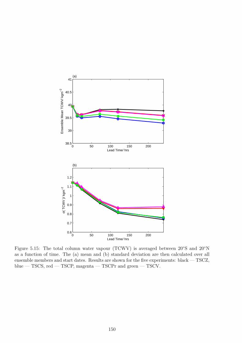
0 50 100 150 20038.5
39
39.5
40
40.5
41(a)
Lead Time/ hrs
Ens
embl
e M
ean
TC
WV
/ kgm
−2
0 50 100 150 2000.6
0.7
0.8
0.9
1
1.1
1.2
(b)
Lead Time/ hrs
σ( T
CW
V )
/ kgm
−2
Figure 5.15: The total column water vapour (TCWV) is averaged between 20◦S and 20◦Nas a function of time. The (a) mean and (b) standard deviation are then calculated over allensemble members and start dates. Results are shown for the five experiments: black — TSCZ,blue — TSCS, red — TSCP, magenta — TSCPr and green — TSCV.
150

(defined in Table 5.3) does not lead to increased bias in T850, U850, Z500 or U200, indicating
that systematic errors in these fields have not increased. An increase in ensemble spread is
observed when the perturbed parameter schemes are used to represent uncertainty in convection
instead of SPPT, and the TSCP/TSCPr forecasts have significantly the largest spread for
T850, U850 and Z500 forecasts, which Figure 5.7 indicates is flow-dependent. The perturbed
parameter schemes produce significantly the most skilful forecasts of T850, U850 and Z500 as
ranked by the RPSS, IGNSS and ESS.
These results indicate that using a fixed perturbed parameter ensemble instead of SPPT
improves the representation of uncertainty in convection. However, the fixed perturbed para-
meter ensembles remain under-dispersive. While an increase in spread is observed when the
perturbed parameter schemes are used to represent uncertainty in convection compared to
SPPT, a substantial proportion of this increase is also observed in Figure 5.6 when SPPT is
switched off for the convection scheme (this counter-intuitive result is analysed in Chapter 6).
Since SPPT is switched off for convection in TSCP and TSCPr, this indicates that the para-
meter perturbations are contributing only slightly to the spread of the ensemble, and much of the
spread increase can be attributed to this decoupling of the convection scheme from SPPT (see
Section 6.5 for further experiments which confirm this “decoupling” hypothesis). The small
impact of the perturbed parameter scheme indicates that such schemes are not fully capturing
the uncertainty in the convection scheme at weather forecasting time scales. This is surprising
as the parameter uncertainty has been explicitly measured and used to develop the scheme.
The TSCPv scheme had a positive impact on the skill of the weather forecasts, and sig-
nificantly improved over the TSCZ and TSCS forecasts for many diagnostics. The impact
on spread and skill was smaller than the static perturbed parameter schemes. It is possible
that the parameter perturbations vary on too fast a time scale for a significant impact to be
observed — if the parameters varied more slowly, a larger, cumulative effect could be observed
in the forecasts. It would be interesting to test the TSCPv scheme using a longer correlation
time scale to test this hypothesis.
The two types of perturbed parameter scheme presented here represent fundamentally dif-
ferent error models. Fixed perturbed parameter schemes are based on the ansatz that there
exists some optimal (or “correct”) value of the parameters in the deterministic parametrisa-
tion scheme. Even using EPPES, the optimal parameters cannot be known with certainty,
151

so a perturbed parameter ensemble samples from a set of likely parameter values. The fixed
perturbed parameter ensembles tested in this chapter were under-dispersive, and did not fully
capture the uncertainty in the forecasts. This indicates that fixed parameter uncertainty is
not the only source of model uncertainty, and that fixed perturbed parameter ensembles cannot
be used alone to represent model uncertainty in an atmospheric simulation. While parameter
uncertainty could account for systematic errors in the forecast, the results indicate that some
component of the error cannot be captured by a deterministic uncertainty scheme. In par-
ticular, perturbed parameter ensembles are unable to represent structural uncertainty due to
the choices made when developing the parametrisation scheme, and a different approach is
required to represent uncertainties due to the bulk formula assumption.
The second error model recognises that in atmospheric modelling there is not necessarily a
“correct” value for the parameters in the physics parametrisation schemes. Instead there exists
some optimal distribution of the parameters in a physical scheme. Since in many cases the
parameters in the physics schemes have no direct physical interpretation, but represent a group
of interacting processes, it is likely that their optimal value may vary from day to day, or from
grid box to grid box, or on larger scales they may be seasonally or latitudinally dependent.
A stochastically perturbed parameter ensemble represents this parameter uncertainty. The
stochastically perturbed parameter scheme also underestimated the error in the forecasts. Even
generalised to allow varying parameters, parameter uncertainty is not the only source of model
uncertainty in weather forecasts. Not all sub-grid scale processes can be accurately represented
using a statistical parametrisation scheme, and some forecast errors cannot be represented
using the phase space of the parametrised tendencies.
The EPPES indicated that the uncertainty in the convection parameters was moderate, and
smaller than expected (Heikki Jarvinen, pers. comm., 2013). The results presented here also
indicate larger parameter perturbations could be necessary to capture the uncertainty in the
forecast from the convection scheme. However, the average tropical total column water vapour
indicates that even these moderate perturbations are sufficient for biases to develop in this field
over the ten day forecast period. The ensemble members with different sets of parameters have
vastly different behaviours, with some showing a systematic drying and others a systematic
moistening in this region. This is very concerning. The second diagnostic presented indicates
that TSCPr also has the problem of systematic drying or moistening for individual ensemble
152

members depending on the model parameters, and suggests that this is a fundamental prob-
lem with using a fixed perturbed parameter ensemble. The fact that this problem develops
noticeably over a ten day window indicates that this could be a serious problem in climate
prediction, where longer forecasts could result in even larger biases developing. This result
supports the conclusions made in Chapter 3 in the context of L96, where individual perturbed
parameter ensemble members were observed to have vastly different regime behaviour. The
TSCPv forecasts did not develop biases in this way, as the parameter sets for each ensemble
member varied over the course of the forecast, which did not allow these biases to develop.
Therefore, stochastically varying perturbed parameter ensembles could be an attractive way
of including parameter uncertainty into weather and climate forecasts.
A particularly interesting and counter-intuitive result is that removing the stochastic per-
turbations from the convection tendency resulted in an increase in forecast spread for some
variables. This is observed for T850, U850 and TCWV in both regions considered, and for
Z500 and U200 in non-convecting regions. SPPT perturbs the sum of the physics tendencies.
It does not represent uncertainty in individual tendencies, but assumes uncertainty is propor-
tional to the total tendency. The increase in spread for TSCZ forecasts compared to TSCS
forecasts suggests that convection could act to reduce the sum of the tendencies, resulting in a
smaller SPPT perturbation. This is as expected from the formulation of the parametrisation
schemes in the IFS, and will be discussed further in Section 6.1. Perturbing each physics tend-
ency independently would allow for an estimation of the uncertainty in each physics scheme,
potentially improving the overall representation of model uncertainty. This is the subject of
the next chapter.
Despite the reduced spread, the TSCS scheme outperforms the TSCZ scheme according
to other forecast diagnostics. The error in T850 forecasts is reduced using the TSCS scheme,
reflected by higher skill scores for this variable, and TSCS is significantly more skilful than
TSCZ at lead times of up to 3 days for U850 and Z500. Additionally, TSCS results in an
increase of spread for U200 and convective precipitation compared to TSCZ. At this point, it
is important to remember that the parametrisation tendencies are not scalar quantities, but are
vectors of values corresponding to the tendency at different vertical levels, and that SPPT uses
the same stochastic perturbation field at each vertical level3. The convection parametrisation
3The perturbation is constant vertically except for tapering in the boundary layer and the stratosphere.
153

scheme is sensitive to the vertical distribution of temperature and humidity, and it is possible
that the tendencies output by the convection parametrisation scheme act to damp or excite
the scheme at subsequent time steps. Therefore perturbing the convective (vector) tendency
using SPPT could lead to an increased variability in convective activity between ensemble
members through amplification of this excitation process. Since both U200 and convective
precipitation are directly sensitive to the convection parametrisation scheme, these variables
are able to detect this increased variability, and show an increased ensemble spread as a result.
In fact, TSCS has significantly the most skilful forecasts out of all five experiments between
days three and ten for U200, and between days three and five for convective precipitation.
T850, U850 and Z500 are less sensitive to convection than U200 and precipitation. Since in
general the total perturbed tendency is reduced for TSCS compared to TSCZ, this could lead
to the reduction in ensemble spread observed for these variables.
The experiments presented in this chapter have used the IFS at a resolution of T159. This
is significantly lower than the operational resolution of T639. Nevertheless, the experiments
give a good indication of what the impact of the different schemes would be on the skill of
the operational resolution IFS. In Chapter 6, results are presented for T159 experiments which
were repeated at T639; the same trends can be observed at the higher resolution. Therefore,
the low resolution runs presented in this chapter can be used to indicate the expected results of
the models at T639, and can suggest whether it would be interesting to run further experiments
at higher resolution.
154

6
Experiments in the IFS:
Independent SPPT
The only relevant test of the validity of a hypothesis is comparison of prediction with
experience.
– Milton Friedman, 1953
6.1 Motivation
The generalised stochastically perturbed parametrisation tendencies (SPPT) scheme developed
in the previous chapter allowed the SPPT perturbation to be switched off for the convection
tendency and replaced with a perturbed parameter scheme. However, it also enables one
to perturb the five IFS physics schemes with independent random fields. In the operational
SPPT, the uncertainty is assumed to be proportional to the total net tendency, whereas this
generalisation to SPPT assumes that the errors from the different parametrisation schemes
are uncorrelated, and that the uncertainty in the forecast is proportional to the individual
tendencies.
The standard deviation of the perturbed tendency, σtend, using operational SPPT is given
by
σ2tend = σ2
n
(5∑
i=1
Pi
)2
, (6.1)
where σn is the standard deviation of the noise perturbation and Pi is the parametrised tend-
ency from the ith physics scheme. This can be compared to the standard deviation using
155

independent SPPT (SPPTi):
σ2tend =
5∑
i=1
(
σ2i P
2i
)
. (6.2)
If the physics tendencies tend to act in opposite directions, SPPTi will acknowledge the large
uncertainty in the individual tendencies and will increase the forecast ensemble spread.
A priori, it is not known whether SPPT or SPPTi is the more physically plausible error
model for the IFS, though it is very unlikely that uncertainties in the different processes are
precisely correlated, as modelled by SPPT. However, the different physics schemes in the
IFS have been developed in tandem, and are called sequentially in the IFS to maintain a
balance. For example, the cloud and convection schemes model two halves of the same set of
atmospheric processes, as described in Section 5.2.1. The convection parametrisation scheme
represents the warming due to moist convection, but the cloud scheme calculates the cooling
due to evaporation of cloudy air that has been detrained from the convective plume. This
means that the net tendency from the two schemes is smaller than each individual tendency,
and SPPT represents a correspondingly small level of uncertainty. SPPTi could be beneficial
in this case, as it is able to represent the potentially large errors in each individual tendency.
On the other hand, if the two schemes have been closely tuned to each other, potentially with
compensating errors, decoupling the two schemes by using independent perturbations could
reduce the forecast skill and introduce errors into the forecasts.
The impact of using SPPTi in the IFS will be tested in this chapter. As a first attempt,
each independent random number field will have the same characteristics as the field used
operationally in SPPT, i.e. each of the five independent fields is itself a composite of three
independent fields with differing temporal and spatial correlations and magnitudes (see Sec-
tion 5.3). A series of experiments is carried out in the IFS. Four experiments are considered
to investigate the impact of the SPPTi scheme, and are detailed in Table 6.1. The impact of
the operational SKEB scheme is also considered as a benchmark. The same resolution, start
dates and lead time were used as in Chapter 5.
Firstly, the impact of SPPTi on global diagnostics is presented in Section 6.2. In Sec-
tion 6.3, the impact of the SPPTi scheme in the tropics is considered, including differences
between behaviour of the scheme in the tropical regions with significant and little convection
which were defined in Chapter 5. The impact of the scheme on the skill of convection dia-
gnostics is presented in Section 6.4. A series of experiments are described in Section 6.5, which
156

Experiment Abbreviation SPPT SPPTi SKEBTSCS ON OFF OFFTSCS + SKEB ON OFF ONTSCSi OFF ON OFFTSCSi + SKEB OFF ON ON
Table 6.1: The four experiments and their abbreviations considered in this chapter to investig-ate the impact of independent SPPT over operational SPPT. The impact of the SKEB schemeis also considered for comparison. See Table 5.3 for an explanation of the abbreviations.
aim to increase understanding of the mechanisms by which SPPTi impacts the ensemble. In
Section 6.6, the results from experiments at operational T639 resolution are presented. In
Section 6.7, the results are discussed and some conclusions are drawn.
6.2 Global Diagnostics
The representations of model uncertainty considered in Chapter 5 focused on the convection
scheme only, so the different schemes were verified in the tropics where convection is most
active. The SPPTi scheme discussed in this chapter affects all parametrisation schemes, so
has a global impact. It is therefore important to evaluate the impact of the scheme on global
forecasts. The global bias, calculated following (1.24) is shown as a percentage in Figure 6.1.
Globally, the bias is small for each variable considered. However, for all variables, implementing
the SPPTi scheme results in an increase in global bias. The impact is particularly large for
U200, where the global bias has more than doubled in magnitude. The impact of SKEB
(comparing blue with cyan, and red with magenta) is considerably smaller than the impact of
the SPPTi scheme (comparing the warm and cool pairs of lines).
Figure 6.2 shows the temporal evolution of the RMS ensemble spread and error respectively,
for each experiment considered, averaged over each standard ECMWF region: the northern
extra-tropics is defined as north of 25◦N , the southern extra-tropics is defined as south of 25◦S,
and the tropics is defined as 25◦S − 25◦N . In the northern and southern extra-tropics (first
and third columns respectively), the impact of SPPTi on the ensemble spread is comparable
to, but slightly smaller than, the impact of SKEB, and all experiments have under-dispersive
forecasts. The different schemes have little impact on the RMSE. However in the tropics (centre
column), SPPTi has a significant positive impact on the spread of the ensemble forecasts. The
impact is significantly larger than that of SKEB, and corrects the under-dispersive forecasts for
157

0 50 100 150 200
−0.2
−0.15
−0.1
−0.05
0
lead time / hrs
% B
ias
(a)(a)(a)(a) T 850
0 50 100 150 200
−1.2
−1
−0.8
−0.6
−0.4
−0.2
0
0.2
lead time / hrs
% B
ias
(b)(b)(b)(b) U 850
0 50 100 150 200
−0.15
−0.1
−0.05
0
lead time / hrs
% B
ias
(c)(c)(c)(c) Z 500
0 50 100 150 2000
0.5
1
1.5
2
2.5
3
lead time / hrs
% B
ias
(d)(d)(d)(d) U 200
Figure 6.1: Global forecast bias as a function of time for (a) T850, (b) U850, (c) Z500 and (d)U200. Results are shown for the four experiments: blue — TSCS; cyan — TSCS + SKEB; red— TSCSi; magenta — TSCSi + SKEB. The bias is calculated as described in the text, andgiven as a percentage of the root mean square of the verification in the region of interest.
T850, U850 and U200. While SPPTi has a larger impact on the spread of Z500 forecasts than
SKEB, the ensembles remain under-dispersive. A small impact on the RMSE is observed —
the T850 and Z500 errors are slightly increased and the U850 and U200 errors slightly reduced
by the SPPTi scheme. These results are very positive, and indicate the potential of the SPPTi
scheme.
Figure 6.2 indicates that SPPTi has the largest impact in the tropics. Figure 6.3 shows
the skill of the forecasts in this region evaluated using the RPSS, IGNSS and ESS for the four
variables of interest. IGNSS indicates an improvement of skill for all variables when SPPTi is
implemented. This is as expected from Figure 6.2: IGNSS strongly penalises under-dispersive
ensemble forecasts, so reducing the degree of under-dispersion results in an improved score.
RPSS and ESS indicate a slight improvement in skill for the U850 and U200 forecasts, but a
slight reduction in skill for the T850 and Z500 forecasts when the SPPTi scheme is used. This
could be due to the increase in root mean square error observed for these variables, linked to
the increase in bias observed in Figure 6.1. The IFS is such a highly tuned forecast model that
it would be very surprising if a newly proposed scheme resulted in an improvement in skill for
all variables in all areas. Before operationally implementing a new scheme, the scheme would
158

0 100 200
1
1.5
2
2.5
3
3.5
lead time / hrs
RM
S(a)
0 100 2000.6
0.8
1
1.2
1.4
1.6
lead time / hrs
RM
S
(b)
0 100 200
1
2
3
4
lead time / hrs
RM
S
(c)
0 100 2001
2
3
4
5
lead time / hrs
RM
S
(d)
0 100 200
1.5
2
2.5
3
3.5
lead time / hrs
RM
S(e)
0 100 200
2
4
6
8
lead time / hrs
RM
S
(f)
0 100 200
200
400
600
lead time / hrs
RM
S
(g)
0 100 200
50
100
150
200
lead time / hrs
RM
S
(h)
0 100 200
200
400
600
800
1000
lead time / hrs
RM
S(i)
0 100 200
2
4
6
8
10
lead time / hrs
RM
S
(j)
0 100 2002
4
6
8
lead time / hrs
RM
S
(k)
0 100 200
2
4
6
8
10
12
lead time / hrs
RM
S
(l)
Figure 6.2: Temporal evolution of the RMS ensemble spread (dashed lines) and RMSE (solidlines) for each standard ECMWF region. First column: northern extra-tropics, north of 25N.Second column: tropics, 25S–25N. Third column: southern extra-tropics, south of 25S. (a)–(c)T850, (d)–(f) U850, (g)–(i) Z500 and (j)–(l) U200. Results are shown for the four experiments:blue — TSCS; cyan — TSCS + SKEB; red — TSCSi; magenta — TSCSi + SKEB.
159

need to be tuned, and the model re-calibrated to account for the effects of the new scheme.
However, the significant improvement in spread observed in the tropics is sufficient to merit
further investigation.
6.3 Effect of Independent SPPT in Tropical Areas
What is the cause of the improved spread in the tropics when the SPPTi scheme is implemen-
ted? As in Chapter 5, let us consider areas in the tropics where there is little convection, and
areas where convection is the dominant process. The regions defined in Section 5.5.1 will be
used as before.
The percentage bias as a function of lead time is shown for areas of little convection in
Figure 6.4. The SPPTi forecasts have a larger bias at lead times greater than 24 hrs for T850
than for operational SPPT, and similar bias characteristics for Z500. However, U850 and U200
both show a reduction in the forecast bias when the SPPTi scheme is used compared to the
operational SPPT scheme. Figure 6.5 shows the same diagnostic for regions with significant
convection. The results are similar for T850 and Z500. U850 shows a slight improvement,
but U200 indicates that SPPTi results in a small increase in bias. For operational SPPT,
the negative bias in non-convecting regions cancels the positive bias in convecting regions to
produce a small globally averaged bias. The SPPTi scheme has effectively reduced the negative
bias in non-convecting regions, but has not had a large impact on the bias in convecting regions,
resulting in the large increase in magnitude of the bias observed for global U200 in Figure 6.1(d).
Considering regionally averaged bias can be misleading due to compensating errors.
Figures 6.6 and 6.7 show the evolution of the RMSE (solid lines) and RMS spread (dashed
lines) for the tropical regions with little convection and with significant convection respectively.
The operational SPPT ensembles (blue lines) are under-dispersive at all times, for all variables,
in both regions. The under-dispersion is greater in regions with significant convection. Includ-
ing SKEB (cyan lines) does not significantly increase the spread of the ensemble.
In regions with little convection, using SPPTi results in a moderately large correction to
this under-dispersion, approximately halving the difference between spread and error for T850,
U850 and U200 when compared to the operational runs. The impact is larger than the impact
of including SKEB. The impact on spread is smaller for Z500, but still positive.
For regions with significant convection, the improvement in spread is greater than in regions
160

0 100 200
0.5
0.6
0.7
0.8
lead time / hrs
RP
SS
(a)(a)(a)(a)
0 100 2000.2
0.3
0.4
0.5
0.6
lead time / hrs
IGN
SS
(b)(b)(b)(b)
0 100 2000.95
0.96
0.97
0.98
0.99
1
lead time / hrs
ES
S
(c)(c)(c)(c)
0 100 200
0.4
0.5
0.6
0.7
0.8
lead time / hrs
RP
SS
(d)(d)(d)(d)
0 100 2000
0.2
0.4
0.6
lead time / hrs
IGN
SS
(e)(e)(e)(e)
0 100 200
0.8
0.85
0.9
0.95
1
lead time / hrs
ES
S
(f)(f)(f)(f)
0 100 200
0.2
0.4
0.6
0.8
lead time / hrs
RP
SS
(g)(g)(g)(g)
0 100 200
−0.2
0
0.2
0.4
lead time / hrs
IGN
SS
(h)(h)(h)(h)
0 100 200
0.8
0.85
0.9
0.95
1
lead time / hrs
ES
S
(i)(i)(i)(i)
0 100 200
0.6
0.7
0.8
0.9
lead time / hrs
RP
SS
(j)(j)(j)(j)
0 100 2000.2
0.4
0.6
0.8
lead time / hrs
IGN
SS
(k)(k)(k)(k)
0 100 2000.92
0.94
0.96
0.98
1
lead time / hrs
ES
S
(l)(l)(l)(l)
Figure 6.3: Ensemble forecast skill scores calculated for the tropics (25S–25N). First column:Ranked Probability Skill Score. Second column: Ignorance Skill Score. Third column: Error-spread Skill Score. (a)–(c) T850, (d)–(f) U850, (g)–(i) Z500 and (j)–(l) U200. Results are shownfor the four experiments: blue — TSCS; cyan — TSCS + SKEB; red — TSCSi; magenta —TSCSi + SKEB.
161

0 50 100 150 200
−0.3
−0.25
−0.2
−0.15
−0.1
−0.05
0
0.05
lead time / hrs
% B
ias
(a)(a)(a)(a) T 850
0 50 100 150 200
−2
0
2
4
6
8
10
lead time / hrs
% B
ias
(b)(b)(b)(b) U 850
0 50 100 150 200−0.2
−0.15
−0.1
−0.05
0
0.05
lead time / hrs
% B
ias
(c)(c)(c)(c) Z 500
0 50 100 150 200
−10
−8
−6
−4
−2
0
2
lead time / hrs
% B
ias
(d)(d)(d)(d) U 200
Figure 6.4: Percentage forecast bias in tropical regions with little convection as a function oftime for (a) T850, (b) U850, (c) Z500 and (d) U200. Results are shown for the four experiments:blue — TSCS; cyan — TSCS + SKEB; red — TSCSi; magenta — TSCSi + SKEB. The biasis calculated as described in the text, and given as a percentage of the root mean square of theverification in the region of interest.
0 50 100 150 200−0.2
−0.15
−0.1
−0.05
0
0.05
lead time / hrs
% B
ias
T 850(a)(a)(a)(a)
0 50 100 150 200−20
−15
−10
−5
0
lead time / hrs
% B
ias
U 850(b)(b)(b)(b)
0 50 100 150 200−0.25
−0.2
−0.15
−0.1
−0.05
0
lead time / hrs
% B
ias
Z 500(c)(c)(c)(c)
0 50 100 150 2000
5
10
15
20
lead time / hrs
% B
ias
U 200(d)(d)(d)(d)
Figure 6.5: As for Figure 6.4, except for tropical regions with significant convection.
162

0 50 100 150 200
1
1.2
1.4
1.6
1.8
2
2.2
2.4
lead time / hrs
RM
S
(a) T 850
0 50 100 150 200
1.5
2
2.5
3
3.5
lead time / hrs
RM
S
(b) U 850
0 50 100 150 200
40
60
80
100
120
140
160
180
lead time / hrs
RM
S(c) Z 500
0 50 100 150 200
2
3
4
5
6
7
8
lead time / hrs
RM
S
(d) U 200
Figure 6.6: Temporal evolution of RMS ensemble spread (dashed lines) and RMSE (solid lines)for tropical regions with little convection for (a) T850, (b) U850, (c) Z500 and (d) U200.Results are shown for the four experiments: blue — TSCS; cyan — TSCS + SKEB; red —TSCSi; magenta — TSCSi + SKEB.
of little convection, whereas the improvement due to SKEB remains small. The spread of the
ensembles closely matches the RMSE, and is slightly over-dispersive for U850. Moreover,
the temporal evolution of the spread has an improved profile for T850, U850 and U200. For
operational SPPT, the increase in spread is a fairly linear function of time, whereas for SPPTi,
there is an initial period of rapid spread increase, followed by a reduction in rate, which closely
matches the observed error growth. Figures 6.6 and 6.7 also indicate that it is the convectively
active regions that are primarily responsible for the observed increase in RMSE for T850 and
Z500 for the SPPTi experiments. This increase in error is a concern.
The RMS error-spread graphical diagnostic gives more information about the calibration
of the forecast, testing whether the ensemble is able to skilfully indicate flow dependent uncer-
tainty. Figures 6.8 and 6.9 show this diagnostic for tropical regions with little and significant
convection respectively, for each variable of interest, at lead times of 1, 3 and 10 days. In both
regions, Z500 is comparatively poorly forecast by the model. The error-spread relationship
is weakly captured, and the ensemble spread is a poor predictor of the expected error in the
ensemble mean. For the other variables, ensemble spread is a good predictor of RMSE in both
regions.
163

0 50 100 150 200
0.4
0.5
0.6
0.7
0.8
0.9
lead time / hrs
RM
S
(a) T 850
0 50 100 150 2001
1.5
2
2.5
3
3.5
lead time / hrs
RM
S
(b) U 850
0 50 100 150 200
40
60
80
100
120
140
160
180
lead time / hrs
RM
S
(c) Z 500
0 50 100 150 2002
3
4
5
6
7
lead time / hrs
RM
S
(d) U 200
Figure 6.7: As for Figure 6.6, except for tropical regions with significant convection.
For the regions with little convection in Figure 6.8, the ensembles appear fairly well cal-
ibrated, and SPPTi has a small positive effect. The largest effect is seen at a lead time of
10 days for U200, where the operational SPPT ensemble was most under-dispersive. For the
regions with significant convection shown in Figure 6.9, forecasts show a large improvement.
The increase in spread of the ensembles is state dependent: for most cases, the increase in
spread results in an improved one-to-one relationship. One exception is Figure 6.9(e), where
the slope of the SPPTi scattered points is too shallow. It is interesting to note that the increase
in RMSE for the T850 forecasts appears to occur predominantly for small error forecasts. This
results in a flat tail to Figures 6.9(a)–(c) at small RMSE and spread, instead of a uniform in-
crease in error across all forecasts. This tail appears to be unique to T850 out of the variables
considered, visible at all lead times, and only in regions where convection dominates.
Figures 6.10 and 6.11 show the skill of the forecasts in regions of little and significant
convection respectively, according to the RPSS, IGNSS and ESS. The skill scores for these
two regions effectively summarise Figures 6.8 and 6.9, and provide more information as to the
source of skill observed in 6.3. In particular:
• The poorer RPSS and ESS for SPPTi in the tropics for T850 (Figure 6.3) is mainly due
to poorer forecast skill in convecting regions, though a small reduction in skill in non-
convecting regions is also observed. The significant improvement in IGNSS in this region
164

0 1 20
0.5
1
1.5
2
2.5
Forecast Spread
RM
SE
(a)
0 1 2 30
1
2
3
Forecast Spread
RM
SE
(b)
0 2 40
1
2
3
4
Forecast Spread
RM
SE
(c)
0 1 20
0.5
1
1.5
2
2.5
Forecast Spread
RM
SE
(d)
0 1 2 30
1
2
3
4
Forecast Spread
RM
SE
(e)
0 2 40
1
2
3
4
5
Forecast Spread
RM
SE
(f)
0 20 400
20
40
60
Forecast Spread
RM
SE
(g)
0 20 40 60 800
50
100
Forecast Spread
RM
SE
(h)
0 100 2000
100
200
300
Forecast Spread
RM
SE
(i)
0 2 40
1
2
3
4
Forecast Spread
RM
SE
(j)
0 2 4 60
2
4
6
8
Forecast Spread
RM
SE
(k)
0 5 100
2
4
6
8
10
Forecast Spread
RM
SE
(l)
Figure 6.8: RMS error-spread diagnostic for tropical regions with little convection for (a)–(c) T850, (d)–(f) U850, (g)–(i) Z500 and (j)–(l) U200, at lead times of 1, 3 and 10 days foreach variable (first, second and third columns respectively). Results are shown for the fourexperiments: blue — TSCS; cyan — TSCS + SKEB; red — TSCSi; magenta — TSCSi +SKEB. The one-to-one diagonal is shown in black.
165

0 0.5 10
0.5
1
Forecast Spread
RM
SE
(a)
0 0.5 1 1.50
0.5
1
1.5
Forecast Spread
RM
SE
(b)
0 0.5 1 1.50
0.5
1
1.5
2
Forecast Spread
RM
SE
(c)
0 1 2 30
1
2
3
Forecast Spread
RM
SE
(d)
0 2 40
1
2
3
4
Forecast Spread
RM
SE
(e)
0 2 4 60
2
4
6
Forecast Spread
RM
SE
(f)
0 20 40 600
20
40
60
80
Forecast Spread
RM
SE
(g)
0 50 1000
50
100
150
200
Forecast Spread
RM
SE
(h)
0 100 2000
50
100
150
200
250
Forecast Spread
RM
SE
(i)
0 2 40
1
2
3
4
5
Forecast Spread
RM
SE
(j)
0 2 4 60
2
4
6
Forecast Spread
RM
SE
(k)
0 5 100
2
4
6
8
10
Forecast Spread
RM
SE
(l)
Figure 6.9: As for Figure 6.8, except for tropical regions with significant convection.
166

0 100 2000.4
0.5
0.6
0.7
0.8
lead time / hrs
RP
SS
(a)(a)(a)(a)
0 100 2000.1
0.2
0.3
0.4
0.5
0.6
lead time / hrs
IGN
SS
(b)(b)(b)(b)
0 100 200
0.9
0.95
1
lead time / hrs
ES
S
(c)(c)(c)(c)
0 100 2000.2
0.3
0.4
0.5
0.6
0.7
lead time / hrs
RP
SS
(d)(d)(d)(d)
0 100 2000
0.1
0.2
0.3
0.4
lead time / hrs
IGN
SS
(e)(e)(e)(e)
0 100 2000.4
0.6
0.8
1
lead time / hrs
ES
S
(f)(f)(f)(f)
0 100 2000.2
0.4
0.6
0.8
lead time / hrs
RP
SS
(g)(g)(g)(g)
0 100 200−0.2
0
0.2
0.4
0.6
lead time / hrs
IGN
SS
(h)(h)(h)(h)
0 100 2000.75
0.8
0.85
0.9
0.95
1
lead time / hrs
ES
S
(i)(i)(i)(i)
0 100 200
0.5
0.6
0.7
0.8
0.9
lead time / hrs
RP
SS
(j)(j)(j)(j)
0 100 200
0.2
0.4
0.6
0.8
lead time / hrs
IGN
SS
(k)(k)(k)(k)
0 100 2000.8
0.85
0.9
0.95
1
lead time / hrs
ES
S
(l)(l)(l)(l)
Figure 6.10: Ensemble forecast skill scores calculated for tropical regions with little convec-tion. First column: Ranked Probability Skill Score. Second column: Ignorance Skill Score.Third column: Error-spread Skill Score. (a)–(c) T850, (d)–(f) U850, (g)–(i) Z500 and (j)–(l)U200. Results are shown for the four experiments: blue — TSCS; cyan — TSCS + SKEB;red — TSCSi; magenta — TSCSi + SKEB.
167
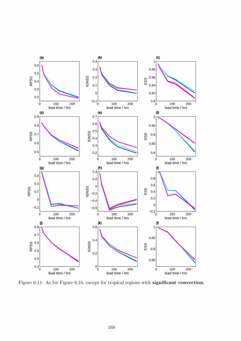
0 100 200
0.2
0.3
0.4
0.5
0.6
lead time / hrs
RP
SS
(a)(a)(a)(a)
0 100 200−0.1
0
0.1
0.2
0.3
0.4
lead time / hrs
IGN
SS
(b)(b)(b)(b)
0 100 2000.9
0.92
0.94
0.96
0.98
1
lead time / hrs
ES
S
(c)(c)(c)(c)
0 100 200
0.5
0.6
0.7
0.8
0.9
lead time / hrs
RP
SS
(d)(d)(d)(d)
0 100 200
0.2
0.3
0.4
0.5
0.6
0.7
lead time / hrs
IGN
SS
(e)(e)(e)(e)
0 100 200
0.8
0.85
0.9
0.95
1
lead time / hrs
ES
S
(f)(f)(f)(f)
0 100 200
−0.2
0
0.2
0.4
0.6
lead time / hrs
RP
SS
(g)(g)(g)(g)
0 100 200
−0.6
−0.4
−0.2
0
0.2
0.4
lead time / hrs
IGN
SS
(h)(h)(h)(h)
0 100 200−0.2
0
0.2
0.4
0.6
0.8
lead time / hrs
ES
S
(i)(i)(i)(i)
0 100 2000.3
0.4
0.5
0.6
0.7
0.8
lead time / hrs
RP
SS
(j)(j)(j)(j)
0 100 2000
0.2
0.4
0.6
lead time / hrs
IGN
SS
(k)(k)(k)(k)
0 100 200
0.85
0.9
0.95
1
lead time / hrs
ES
S
(l)(l)(l)(l)
Figure 6.11: As for Figure 6.10, except for tropical regions with significant convection.
168
indicates an improvement in ensemble spread as observed, so it is likely this reduction in
RPSS and ESS is due to the increased RMSE and the flat tail observed in the RMSE-
spread diagnostic plots.
• The significantly improved RPSS and ESS for SPPTi for U850 is due to improved skill in
convecting regions. The improvements in IGNSS involve contributions from both regions.
• Z500 is not a particularly informative field to study in the tropics as it is very flat and
featureless. IGNSS indicates negative skill for lead times greater than 3 days, and RPSS
and ESS also indicate little skill for this variable.
• The improvement of RPSS and IGNSS for U200 in the tropics is mostly due to an
improved forecast skill in the regions with little convection. This improvement was clearly
visible in the RMSE-spread scatter diagrams. A small but significant improvement in
skill in convecting regions is also observed, especially at later lead times.
6.4 Convection Diagnostics
The impact of SPPTi is largest in regions with significant convection. To investigate if this
is an indication that convection is modelled better by this scheme, the convection diagnostics
discussed in Chapter 5 will be considered here, evaluated for tropical regions with significant
convection.
6.4.1 Precipitation
Firstly, the skill of forecasting convective precipitation is considered. Convective precipitation
is calculated by the convection scheme, and is not directly perturbed by SPPT. Therefore any
impact of SPPTi on forecasting this variable indicates a feedback mechanism: the convection
physics scheme is responding to the altered atmospheric state. As in Chapter 5, the GPCP data
set is used for verification of precipitation. Figure 6.12 shows the RMS error-spread diagnostic
for convective precipitation. It indicates that operational SPPT is under-dispersive for this
variable, and that SPPTi results in an improved spread in forecast convective precipitation at
all lead times. Figure 6.13 shows (a) the bias, (b) the RMSE and spread as a function of time,
and (c)–(e) the forecast skill scores for convective precipitation. The bias in the convective
169

0 0.005 0.010
0.005
0.01
0.015
Forecast Spread
RM
SE
(a)
0 0.005 0.01 0.0150
0.005
0.01
0.015
Forecast SpreadR
MS
E
(b)
0 0.005 0.01 0.0150
0.005
0.01
0.015
Forecast Spread
RM
SE
(c)
Figure 6.12: RMS error-spread diagnostic for cumulative convective precipitation for the 24hour window before a lead time of (a) 1 day, (b) 3 days and (c) 10 days. The diagnostic iscalculated for tropical regions with significant convection. Results are shown for the fourexperiments: blue — TSCS; cyan — TSCS + SKEB; red — TSCSi; magenta — TSCSi +SKEB. The one-to-one diagonal is shown in black.
0 100 200
0
2
4
6
8
lead time / hrs
% B
ias
(a)(a)(a)(a)
0 100 2004
5
6
7
8
x 10−3
lead time / hrs
RM
S
(b)
0 100 200
0.1
0.15
0.2
0.25
lead time / hrs
RP
SS
(c)(c)(c)(c)
0 100 200
−0.25
−0.2
−0.15
−0.1
−0.05
0
lead time / hrs
IGN
SS
(d)(d)(d)(d)
0 100 2000.1
0.2
0.3
0.4
0.5
0.6
0.7
lead time / hrs
ES
S
(e)(e)(e)(e)
Figure 6.13: Summary forecast diagnostics for 24 hour cumulative convective precipitation intropical regions with significant convection. (a) Percentage bias. (b) Temporal evolutionof RMS ensemble spread (dashed lines) and error (solid lines) averaged over the region. (c)Ranked Probability Skill Score (d) Ignorance Skill Score. (e) Error-spread Skill Score. Resultsare shown for the four experiments: blue — TSCS; cyan — TSCS + SKEB; red — TSCSi;magenta — TSCSi + SKEB
170

precipitation forecasts is higher for SPPTi than for SPPT, but all other diagnostics indicate
that the SPPTi forecasts are more skilful than the operational SPPT forecasts.
The skill of the precipitation forecasts can also be evaluated by considering the spatial
distribution of cumulative precipitation (convective plus large-scale) for the different forecast
models. The average 24-hour cumulative precipitation is shown for the GPCP data set in
Figure 6.14. The difference between the forecast and GPCP fields is shown in Figure 6.15 for
each of the four experiments in Table 6.1. Blue indicates the forecast has too little precipitation
whereas red indicates too much precipitation. Figures (a) and (b) show the results for the
operational SPPT scheme, with and without SKEB respectively. The results are very similar.
Both show too much precipitation across the oceans. Figures (c) and (d) show the results for
the SPPTi scheme, with and without SKEB respectively. Again, including SKEB has little
impact, but including the SPPTi scheme has slightly increased the amount of precipitation
over the oceans, as indicated earlier by the increase in bias in Figure 6.13(a). Using SPPTi
does not result in a significant change in the spatial distribution of rain.
The skill of the precipitation forecasts can also be evaluated by considering the global
frequency distribution of rain rate for the different forecast models and comparing to the
observed rain rate distribution in the GPCP dataset. This is shown in Figure 6.16. All four
forecast models perform well, though all underestimate the proportion of low rain rates and
overestimate the proportion of high rain rates. The operational SPPT scheme is closer to the
observations at mid to high rain rates, and the SPPTi scheme is marginally better at low rain
rates. Importantly, the diagnostic does not flag up any major concerns for the new SPPTi:
when SPPT was originally being developed, such a diagnostic showed that very high rain rates
occurred at a significantly inflated frequency, which led to alterations to the SPPT scheme
(Martin Leutbecher, pers. comm., 2013).
6.4.2 Total Column Water Vapour
Secondly, the skill of forecasting total column water vapour (TCWV) is considered, to which
the convection scheme is sensitive. Figure 6.17 shows the RMS error-spread diagnostic for
TCWV. As observed in Section 5.6.2.2, forecasts for this variable are poorly calibrated for
all experiments. They have a systematically too large RMSE, and the RMS error-spread
diagnostic has a shallow slope. Nevertheless, the SPPTi scheme increases the spread of the
171
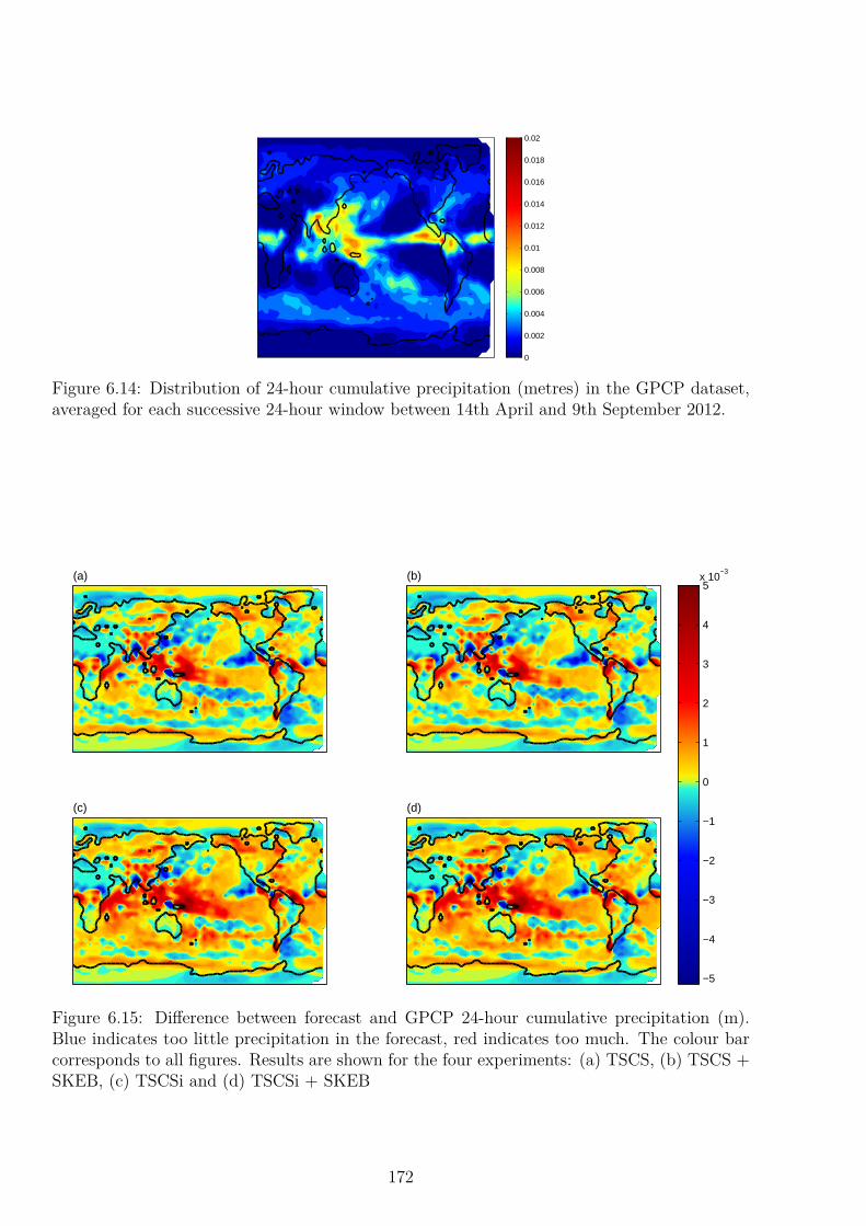
0
0.002
0.004
0.006
0.008
0.01
0.012
0.014
0.016
0.018
0.02
Figure 6.14: Distribution of 24-hour cumulative precipitation (metres) in the GPCP dataset,averaged for each successive 24-hour window between 14th April and 9th September 2012.
(a) (b)
(c)
(d)
−5
−4
−3
−2
−1
0
1
2
3
4
5x 10
−3
Figure 6.15: Difference between forecast and GPCP 24-hour cumulative precipitation (m).Blue indicates too little precipitation in the forecast, red indicates too much. The colour barcorresponds to all figures. Results are shown for the four experiments: (a) TSCS, (b) TSCS +SKEB, (c) TSCSi and (d) TSCSi + SKEB
172

0 50 100 15010
−7
10−6
10−5
10−4
10−3
10−2
10−1
100
Rain Rate / mm in 24 hours
prob
abili
ty
Figure 6.16: Probability distribution of rain rate (mm/12hrs) evaluated globally. The distri-bution has been normalised to 1, given that rain is observed in each 12 hour window. Theobserved result from the GPCP dataset (grey) are compared to TSCS (blue), TSCS + SKEB(cyan), TSCSi (red) and TSCSi + SKEB (magenta) forecasts.
ensemble compared to the operational scheme, improving the calibration. Figure 6.18 shows (a)
the bias, (b) the RMSE and spread as a function of time, and (c)–(e) the forecast skill scores for
TCWV. These diagnostics indicate a significant improvement in forecast skill of TCWV when
SPPTi is used. The forecast bias is reduced, the RMS spread is increased without increasing
the RMSE, and the RPSS, IGNSS and ESS all indicate higher skill.
It is possible that SPPTi could result in significant changes of TCWV in the tropics as
was observed for the perturbed parameter experiments in Chapter 5, so this must be checked.
Figure 6.19 shows the average TCWV between 20◦S and 20◦N (calculated as described in
Section 5.6.2.2). This will diagnose if using SPPTi results in a systematic drying or moistening
of the tropics. All experiments show an initial spin-down period where the tropics dry by
0.5 kgm−2 over the first 12 hours, before stabilising. The operational SPPT forecasts in figures
(a) and (b) show a slight drying over the 240 hour forecast window, whereas the SPPTi forecasts
in figures (c) and (d) have a more constant average TCWV. All four experiments show stable
results.
173

1 2 3 4 5
1
2
3
4
5
Forecast Spread
RM
SE
(a)
(a)
2 4 61
2
3
4
5
6
7
Forecast SpreadR
MS
E(b)
(b)
2 4 6 8
2
4
6
8
Forecast Spread
RM
SE
(c)
(c)
Figure 6.17: RMS error-spread diagnostic for TCWV for lead times of (a) 1 day, (b) 3 days and(c) 10 days. The diagnostic is calculated for tropical regions with significant convection.Results are shown for the four experiments: blue — TSCS; cyan — TSCS + SKEB; red —TSCSi; magenta — TSCSi + SKEB. The one-to-one diagonal is shown in black.
0 50 100 150 200
−2.5
−2
−1.5
−1
lead time / hrs
% B
ias
(a)(a)(a)(a)
0 50 100 150 200
2
3
4
5
6
lead time / hrs
RM
S
(b)
0 50 100 150 2000.1
0.2
0.3
0.4
0.5
0.6
0.7
lead time / hrs
RP
SS
(c)(c)(c)(c)
0 50 100 150 200−0.2
−0.1
0
0.1
0.2
0.3
lead time / hrs
IGN
SS
(d)(d)(d)(d)
0 50 100 150 200
0.65
0.7
0.75
0.8
0.85
0.9
0.95
lead time / hrs
ES
S
(e)(e)(e)(e)
Figure 6.18: Summary forecast diagnostics for TCWV in tropical regions with significantconvection. (a) Percentage bias. (b) Temporal evolution of RMS ensemble spread (dashedlines) and error (solid lines) averaged over the region. (c) Ranked Probability Skill Score (d)Ignorance Skill Score. (e) Error-spread Skill Score. Results are shown for the four experiments:blue — TSCS; cyan — TSCS + SKEB; red — TSCSi; magenta — TSCSi + SKEB
174

0 50 100 150 20038.5
39
39.5
40
40.5(a)
Lead Time/ hrsA
vera
ge T
CW
V/ k
gm−
20 50 100 150 200
38.5
39
39.5
40
40.5(b)
Lead Time/ hrs
Ave
rage
TC
WV
/ kgm
−2
0 50 100 150 20038.5
39
39.5
40
40.5(c)
Lead Time/ hrs
Ave
rage
TC
WV
/ kgm
−2
0 50 100 150 20038.5
39
39.5
40
40.5(d)
Lead Time/ hrsA
vera
ge T
CW
V/ k
gm−
2
Figure 6.19: Average TCWV between 20◦S and 20◦N as a function of time. The spatial averageis calculated for each ensemble member averaged over all start dates, and the averages for eachof the fifty ensemble members are shown. Results are shown for the four experiments: (a)TSCS, (b) TSCS + SKEB, (c) TSCSi, and (d) TSCSi + SKEB.
6.5 Individually Independent SPPT
Independent SPPT assumes that the errors associated with different physics schemes are un-
correlated. It also has the effect of decoupling the physics schemes in the IFS: the random
patterns are introduced after all calculations have been made so each physics scheme does not
have the opportunity to react to the modified tendencies from the other schemes. The results
presented in this chapter show that this assumption results in a large increase of spread, partic-
ularly in convecting regions, and for U200 in non-convecting regions. To probe further into the
mechanisms of SPPTi, a series of five experiments was carried out. In each experiment, just
one of the five physics schemes was perturbed with an independent random number field to the
other four (Table 6.2). These “individually independent SPPT” experiments should indicate
the degree to which a particular physics scheme should have an independent error distribution
from the others. In particular, these experiments aim to answer the following questions:
1. Is it decoupling one particular scheme from the others that results in the large increase
in spread, or is it important that all schemes are treated independently?
2. Does decoupling one particular scheme result in the increased error observed for T850?
175
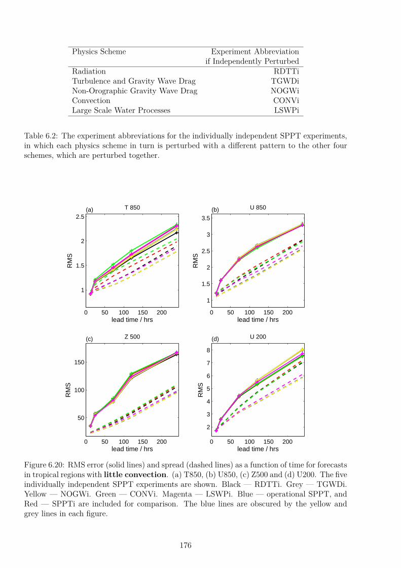
Physics Scheme Experiment Abbreviationif Independently Perturbed
Radiation RDTTiTurbulence and Gravity Wave Drag TGWDiNon-Orographic Gravity Wave Drag NOGWiConvection CONViLarge Scale Water Processes LSWPi
Table 6.2: The experiment abbreviations for the individually independent SPPT experiments,in which each physics scheme in turn is perturbed with a different pattern to the other fourschemes, which are perturbed together.
0 50 100 150 200
1
1.5
2
2.5
lead time / hrs
RM
S
(a) T 850
0 50 100 150 200
1
1.5
2
2.5
3
3.5
lead time / hrs
RM
S
(b) U 850
0 50 100 150 200
50
100
150
lead time / hrs
RM
S
(c) Z 500
0 50 100 150 200
2
3
4
5
6
7
8
lead time / hrs
RM
S
(d) U 200
Figure 6.20: RMS error (solid lines) and spread (dashed lines) as a function of time for forecastsin tropical regions with little convection. (a) T850, (b) U850, (c) Z500 and (d) U200. The fiveindividually independent SPPT experiments are shown. Black — RDTTi. Grey — TGWDi.Yellow — NOGWi. Green — CONVi. Magenta — LSWPi. Blue — operational SPPT, andRed — SPPTi are included for comparison. The blue lines are obscured by the yellow andgrey lines in each figure.
176

Figure 6.20 shows the RMSE in the ensemble mean and RMS ensemble spread as a function
of time for each of the five individually independent SPPT experiments in regions with little
convection. The results for SPPT and SPPTi are also shown for comparison. The largest
impact is observed for U200, where both CONVi and RDTTi show the same spread increase
as SPPTi. This indicates that it is decoupling these two schemes which results in the large
spread increase observed for U200 when SPPTi is used instead of SPPT. For the other variables
considered, the impact of each individually independent scheme is more moderate, though in
each case CONVi and RDTTi result in the largest increase in spread. For T850, RDTTi also
results in a reduction in RMSE when compared to forecasts which use the operational SPPT
scheme.
Apart from for U200, SPPTi has the largest impact in regions with significant convection.
Figure 6.21 shows the RMSE and RMS spread as a function of time in these regions. CONVi
has the largest impact for each variable — perturbing the convection tendencies independently
from the other schemes results in an increase of ensemble spread equal to or greater than
independently perturbing all physics schemes. This supports the results from Chapter 5, in
which it was observed that decoupling the convection scheme by not perturbing its tendencies
resulted in an increase in spread. The next most influential scheme is radiation. For Z500 and
U200, perturbing this scheme independently also results in an increase of ensemble spread equal
to SPPTi. A large impact is also seen for U850 and T850. For the variables at 850 hPa, LSWPi
has a large impact. This is especially true at short lead times, when the impact is greater than
that of radiation. Using independent random fields for TGWDi (grey) and NOGWi (yellow)
has little impact on the ensemble spread — their RMSE and RMS spread are almost identical
to those from the operational SPPT forecasts. This is probably because these two schemes
act mainly in the boundary layer (TGWD) or in the middle atmosphere (NOGW), away from
the variables of interest. Additionally, the stochastic perturbations to these schemes will be
tapered, which will further reduce the impact of SPPTi.
Figure 6.21 also indicates which schemes contribute to the observed increase/decrease in
RMSE for SPPTi in regions with significant convection. For T850, SPPTi resulted in an
increase in RMSE. This same increase is observed for CONVi, and to a lesser extent for the
LSWPi forecasts. For the other variables, CONVi shows a similar RMSE to operational SPPT.
It is interesting to note that the RDTTi experiment does not result in an increase in error for
177

0 50 100 150 200
0.4
0.5
0.6
0.7
0.8
0.9
lead time / hrs
RM
S
(a) T 850
0 50 100 150 2001
1.5
2
2.5
3
3.5
4
lead time / hrs
RM
S
(b) U 850
0 50 100 150 200
40
60
80
100
120
140
160
180
lead time / hrs
RM
S
(c) Z 500
0 50 100 150 2002
3
4
5
6
7
lead time / hrs
RM
S
(d) U 200
Figure 6.21: RMS error (solid lines) and spread (dashed lines) as a function of time for forecastsin tropical regions with significant convection. (a) T850, (b) U850, (c) Z500 and (d) U200.The five individually independent SPPT experiments are shown. Black — RDTTi. Grey —TGWDi. Yellow — NOGWi. Green — CONVi. Magenta — LSWPi. Blue — operationalSPPT, and Red — SPPTi are included for comparison. The blue lines are obscured by theyellow and grey lines in each figure. The black solid line in (a) is obscured by the grey solidline.
178

T850, but does give a substantial increase in spread. The RDTTi experiment also performs
well for U850 and Z500, with an increase in spread and no increase in error observed for both
variables. For U200, the RDTTi scheme results in a decrease in error. These results imply
that much of the spread increase observed with SPPTi could be achieved by perturbing radiation
independently from the other physics schemes, which will not result in the increase in RMSE
for T850.
Figure 6.22 shows the RMS error-spread diagnostic at a lead time of ten days for the
individually independent experiments in regions with significant convection. This diagnostic
confirms that both CONVi (green) and RDTTi (black) produce forecasts with a similar degree
of spread to SPPTi (red). Furthermore, these individually independent schemes improve the
one-to-one relationship between RMSE and RMS spread. Figure 6.22(a) shows the results
for T850, including the increased error for predictable situations. The inset figure shows the
region of interest in more detail, indicated by the grey rectangle. LSWPi results in a significant
increase of error and a flatter ‘tail’. CONVi also results in an increase of error for the smallest
forecast spread cases, giving an upward ‘hook’ in the scatter diagnostic at smallest spreads.
This indicates poorly calibrated forecasts: the forecast spread does not correctly indicate the
error in the ensemble mean, and forecasts with the smallest spreads of between 0.4 and 0.5◦C
consistently have a higher error than those with spreads between 0.5 and 0.6◦C. The results
for RDTTi are positive, showing an increase in spread but no associated increase in error.
Figure 6.23 shows the skill of the individually independent SPPT forecasts in regions with
significant convection, as indicated by the RPSS, IGNSS and ESS. Overall, the RDTTi forecasts
are more skilful than forecasts from any other scheme. In fact, RDTTi is more skilful than
SPPT for T850, whereas SPPTi was less skilful than SPPT for this variable. RDTTi also
performs well for the other variables considered, and has skill equal to or better than the
SPPTi scheme in most cases.
6.6 High Resolution Experiments
Due to limitations in computer resources, the experiments presented above ran the IFS at a
relatively low resolution of T159. The question then arises: does SPPTi have the same impact
when the model is run at the operational resolution of T639? I am grateful to Sarah-Jane Lock
(ECMWF), who ran two experiments on my behalf to test SPPTi at operational resolution.
179

0.5 1 1.5 2
0.5
1
1.5
2
Forecast Spread
RM
SE
(a)
1 2 3 4 5 6
1
2
3
4
5
6
Forecast Spread
RM
SE
(b)
50 100 150
50
100
150
200
250
Forecast Spread
RM
SE
(c)
2 4 6 8 102
4
6
8
10
Forecast Spread
RM
SE
(d)
Figure 6.22: RMS error-spread diagnostic for tropical regions with significant convection for(a) T850, (b) U850, (c) Z500 and (d) U200, at a lead times of 10 days. The five individuallyindependent SPPT experiments are shown (triangles): Black — RDTTi, Grey — TGWDi,Yellow — NOGWi, Green — CONVi, and Magenta — LSWPi. For comparison, the operationalSPPT (blue circles) and SPPTi (red circles) are also shown. The one-to-one diagonal is shownin black. The tiled figure in (a) is a close up of the region indicated by the grey rectangle.
180
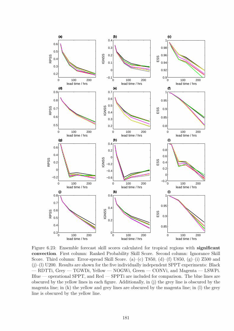
0 100 200
0.2
0.3
0.4
0.5
0.6
lead time / hrs
RP
SS
(a)(a)(a)(a)(a)(a)(a)
0 100 200−0.1
0
0.1
0.2
0.3
0.4
lead time / hrs
IGN
SS
(b)(b)(b)(b)(b)(b)(b)
0 100 2000.9
0.92
0.94
0.96
0.98
1
lead time / hrs
ES
S
(c)(c)(c)(c)(c)(c)(c)
0 100 200
0.5
0.6
0.7
0.8
0.9
lead time / hrs
RP
SS
(d)(d)(d)(d)(d)(d)(d)
0 100 200
0.2
0.3
0.4
0.5
0.6
0.7
lead time / hrs
IGN
SS
(e)(e)(e)(e)(e)(e)(e)
0 100 200
0.8
0.85
0.9
0.95
1
lead time / hrs
ES
S
(f)(f)(f)(f)(f)(f)(f)
0 100 200
−0.2
0
0.2
0.4
0.6
lead time / hrs
RP
SS
(g)(g)(g)(g)(g)(g)(g)
0 100 200
−0.6
−0.4
−0.2
0
0.2
0.4
lead time / hrs
IGN
SS
(h)(h)(h)(h)(h)(h)(h)
0 100 200−0.2
0
0.2
0.4
0.6
0.8
lead time / hrs
ES
S
(i)(i)(i)(i)(i)(i)(i)
0 100 2000.3
0.4
0.5
0.6
0.7
0.8
lead time / hrs
RP
SS
(j)(j)(j)(j)(j)(j)(j)
0 100 2000
0.2
0.4
0.6
lead time / hrs
IGN
SS
(k)(k)(k)(k)(k)(k)(k)
0 100 200
0.85
0.9
0.95
1
lead time / hrs
ES
S
(l)(l)(l)(l)(l)(l)(l)
Figure 6.23: Ensemble forecast skill scores calculated for tropical regions with significantconvection. First column: Ranked Probability Skill Score. Second column: Ignorance SkillScore. Third column: Error-spread Skill Score. (a)–(c) T850, (d)–(f) U850, (g)–(i) Z500 and(j)–(l) U200. Results are shown for the five individually independent SPPT experiments: Black— RDTTi, Grey — TGWDi, Yellow — NOGWi, Green — CONVi, and Magenta — LSWPi.Blue — operational SPPT, and Red — SPPTi are included for comparison. The blue lines areobscured by the yellow lines in each figure. Additionally, in (j) the grey line is obscured by themagenta line; in (k) the yellow and grey lines are obscured by the magenta line; in (l) the greyline is obscured by the yellow line.
181
Ten-day ensemble hindcasts were initialised every five days between 14 April and 18 June
2012 (14 dates in total). The ensembles have 20 members instead of the operational 50. The
two experiments repeated at T639 were “SPPT” and “SPPTi”. A subset of twenty ensemble
members is taken from the operational forecasts for these dates to produce equivalent “SPPT
+ SKEB” forecasts for comparison.
6.6.1 Global Diagnostics
Figure 6.24 shows the RMSE and RMS spread for each of the standard ECMWF global regions
as a function of time for the variables of interest. At this higher resolution, the spread of the
forecasts is well calibrated in the extra-tropics (first and third column). SPPTi has little
impact here, so the ensembles remain well calibrated. In the tropics, the T639 forecasts are
under-dispersive. Here, SPPTi results in a significant increase in spread, and has a larger
impact on ensemble spread than the operational SKEB scheme. These results are similar to
those at T159, shown in Figure 6.2. The key difference between T159 and T639 is that the
operational T639 forecasts are better calibrated than the equivalent T159 forecasts. This means
that when SPPTi is implemented at T639, the ensemble forecasts become over-dispersive for
some variables (e.g. U850). There is also a significant increase in RMSE for T850 and Z500
forecasts at T639. The impact of SPPTi on U200 forecasts is an good match between the
ensemble spread and RMS error in the ensemble mean.
It is important to note that for T850, U850 and U200, the ensemble spread is greater than
the RMSE at a lead time of 12 hours for all experiments. This is indicative of inflation of initial
condition uncertainty to compensate for an incomplete representation of model uncertainty.
Because the ensembles are under-dispersive at longer lead times, the initial condition perturb-
ations have been artificially inflated to increase the ensemble spread. In fact, in the IFS, the
initial condition perturbations calculated by the EDA system are combined with singular vec-
tor perturbations before they are used. If SPPT is replaced by SPPTi, this artificial inflation
could be removed, and the raw initial condition uncertainty estimated by the EDA system used
instead. The temporal evolution of the ensemble spread for forecasts of U850 closely matches
the evolution of the RMSE (Figure 6.24(e)), and if the initial condition perturbations were
to be reduced to the raw EDA output, the results here indicate that SPPTi could produce a
forecast that is well calibrated at all lead times for this variable. It would also be interesting
182

0 100 200
1
2
3
4
lead time / hrs
RM
S(a)
0 100 2000.6
0.8
1
1.2
1.4
1.6
lead time / hrs
RM
S
(b)
0 100 200
1
2
3
4
lead time / hrs
RM
S
(c)
0 100 2001
2
3
4
5
6
lead time / hrs
RM
S
(d)
0 100 200
1.5
2
2.5
3
3.5
lead time / hrs
RM
S(e)
0 100 200
2
4
6
lead time / hrs
RM
S
(f)
0 100 200
200
400
600
800
lead time / hrs
RM
S
(g)
0 100 200
50
100
150
lead time / hrs
RM
S
(h)
0 100 200
200
400
600
800
1000
lead time / hrs
RM
S(i)
0 100 200
2
4
6
8
10
lead time / hrs
RM
S
(j)
0 100 2002
4
6
8
lead time / hrs
RM
S
(k)
0 100 200
2
4
6
8
10
12
lead time / hrs
RM
S
(l)
Figure 6.24: Temporal evolution of RMS ensemble spread (dashed lines) and RMSE (solidlines) for each standard ECMWF region. First column: northern extra-tropics, north of 25N.Second column: tropics, 25S–25N. Third column: southern extra-tropics, south of 25S. (a)–(c) T850, (d)–(f) U850, (g)–(i) Z500 and (j)–(l) U200. Results are shown for the three T639experiments: blue — TSCS; cyan — TSCS + SKEB; red — TSCSi.
183

to test using SPPTi in the EDA system, as it is possible that using SPPTi will impact the
initial condition uncertainty estimated using the EDA.
6.6.2 Verification in the Tropics
As at T159, SPPTi has the largest impact in the tropics. To investigate the source of the
increased spread, the forecasts will be verified in areas in the tropics where there is little
convection, and in areas where convection is the dominant process. The areas considered will
be those defined in Section 5.5.1. Results are shown in Figures 6.25 and 6.26 for regions with
little and significant convection respectively. The operational forecasts are under-dispersive
in both regions. As at T159, the under-dispersion is more severe in regions with significant
convection. For both regions, SPPTi has the effect of significantly increasing the ensemble
spread, whereas the impact of SKEB is more moderate. However, SPPTi also increases the
RMSE for T850 and Z500 forecasts in both regions, and results in a slight increase of RMSE
for U850 and U200 forecasts in convecting regions. In non-convecting regions, SPPTi results
in a slight reduction in RMSE for U850 and U200. The improved temporal evolution of the
ensemble spread identified above is observed in convecting regions, but not in non-convecting
regions. As at T159, the difference in behaviour between convecting and non-convecting regions
indicates that it is convection, and its interactions with other physical processes, that is the key
mechanism by which SPPTi affects the ensemble.
Figures 6.27 and 6.28 show the RMS error-spread graphical diagnostic at a lead time of
ten days for the three T639 experiments for regions with little and significant convection
respectively. The forecasts have been binned into 14 bins instead of 30 to ensure the population
of each bin is the same as before, and is a sufficiently large sample to estimate the statistics. The
impact of SPPTi is small in regions with little convection, though the spread error relationship
is improved slightly for U850. The average spread of forecasts is also improved for U200, but
the flow dependent calibration is poor — the scattered points do not follow the one-to-one
line. In regions of significant convection, the impact is greater. For T850 and Z500 there is an
improved error-spread relationship when SPPTi is used instead of SPPT. The spread of the
ensemble forecasts has increased, and the forecasts continue to give a flow-dependent indication
of uncertainty in the forecast. However, for T850, an increase in RMSE is observed. Unlike at
T159, this increase in RMSE occurs for all forecast spreads, not just for the small spread and
184
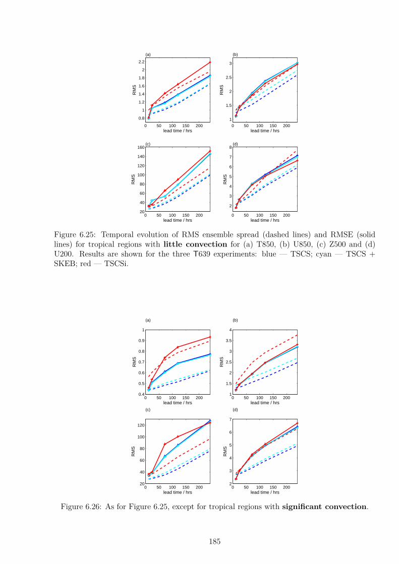
0 50 100 150 200
0.8
1
1.2
1.4
1.6
1.8
2
2.2
lead time / hrsR
MS
(a)
0 50 100 150 200
1
1.5
2
2.5
3
lead time / hrs
RM
S
(b)
0 50 100 150 20020
40
60
80
100
120
140
160
lead time / hrs
RM
S
(c)
0 50 100 150 200
2
3
4
5
6
7
8
lead time / hrsR
MS
(d)
Figure 6.25: Temporal evolution of RMS ensemble spread (dashed lines) and RMSE (solidlines) for tropical regions with little convection for (a) T850, (b) U850, (c) Z500 and (d)U200. Results are shown for the three T639 experiments: blue — TSCS; cyan — TSCS +SKEB; red — TSCSi.
0 50 100 150 2000.4
0.5
0.6
0.7
0.8
0.9
1
lead time / hrs
RM
S
(a)
0 50 100 150 2001
1.5
2
2.5
3
3.5
4
lead time / hrs
RM
S
(b)
0 50 100 150 20020
40
60
80
100
120
lead time / hrs
RM
S
(c)
0 50 100 150 2002
3
4
5
6
7
lead time / hrs
RM
S
(d)
Figure 6.26: As for Figure 6.25, except for tropical regions with significant convection.
185

1 2 3
0.5
1
1.5
2
2.5
3
3.5
Forecast SpreadR
MS
E
(a)
1 2 3 4 5
1
2
3
4
5
Forecast Spread
RM
SE
(b)
50 100 150 200
50
100
150
200
250
Forecast Spread
RM
SE
(c)
2 4 6 8 10 122
4
6
8
Forecast Spread
RM
SE
(d)
Figure 6.27: RMS error-spread diagnostic for tropical regions with little convection for (a)T850, (b) U850, (c) Z500 and (d) U200, at a lead times of 10 days for each variable. Resultsare shown for the three T639 experiments: blue — TSCS; cyan — TSCS + SKEB; red —TSCSi. The one-to-one diagonal is shown in black.
error cases. For U850, SPPTi also increases the spread of the forecasts, but by too great an
amount. For U200, the SPPTi results follow a shallower slope than the SPPT forecast results.
This indicates a reduced degree of flow-dependent predictability, though this is not a problem
at earlier lead times (not shown).
Figures 6.29 and 6.30 show the skill of the ensemble forecasts in regions with little and
significant convection respectively. Despite the improvement in spread, the SPPTi forecasts
tend to score poorly due to an associated increase in RMSE. The SPPTi forecasts are more
skilful than the SPPT forecasts for U850 and U200 in non-convecting regions, and for Z500 at
long lead times in convecting regions according to all skill scores.
6.7 Discussion and Conclusion
SPPTi results in a significant increase of spread for all variables at all lead times. In the extra-
tropics, the ensemble forecasts are well calibrated at T639, and moderately under-dispersive
at T159. The impact of SPPTi is small in these regions. At T159, a small increase in ensemble
spread is observed correcting for the under-dispersion, and at T639 the impact is smaller, and
the ensemble forecasts remain well calibrated. The impact of SPPTi is similar to SKEB in
these regions. In the tropics, forecasts made with SPPT are significantly under-dispersive at
186

0.5 1 1.5
0.5
1
1.5
2
Forecast Spread
RM
SE
(a)
2 4 6
1
2
3
4
5
Forecast Spread
RM
SE
(b)
50 100 150
50
100
150
200
Forecast Spread
RM
SE
(c)
2 4 6 8 10
2
4
6
8
10
Forecast Spread
RM
SE
(d)
Figure 6.28: As for Figure 6.27, except for tropical regions with significant convection.
both T159 and T639. SPPTi has a large beneficial impact in these regions. The forecast
spread is significantly larger than when SPPT is used, and the impact is considerably larger
than the impact of SKEB. This is observed at both T159 and T639. SPPTi produces skilful,
flow-dependent estimates of forecast uncertainty, having a larger impact on forecasts that were
more under-dispersive when using SPPT.
The impact of SPPTi in tropical regions with significant convection (Figure 6.7) is consider-
ably greater than in tropical regions with little convection (Figure 6.6) for T850 and U850, and
to a lesser extent, for Z500. This indicates that convection, together with its interactions with
other physics schemes, is a key process by which SPPTi impacts the ensemble. Equation (6.2)
indicates that the forecast uncertainty represented by SPPTi will only be greater than SPPT
for regions where the model tendencies act in opposite directions, i.e., where the individual
tendencies are large but the net tendency is small. In tropical regions with significant con-
vection, this is indeed the case for the IFS. The convection scheme parametrises the effect of
convective latent heating on the atmosphere. This scheme interacts directly with the large
scale water processes (clouds) scheme: water detrained from the convective plume acts as a
source of water for clouds in the LSWP scheme, which then calculates the effect of evaporative
cooling on the atmosphere (ECMWF, 2012). This interaction means that a warming due to
convection tends to be associated with a cooling from the cloud scheme. The opposing nature
of these tendencies results in the significant increase in ensemble spread associated with SPPTi
187
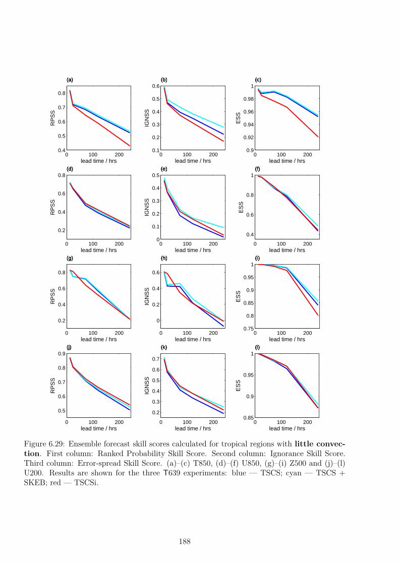
0 100 2000.4
0.5
0.6
0.7
0.8
lead time / hrs
RP
SS
(a)(a)(a)
0 100 2000.1
0.2
0.3
0.4
0.5
0.6
lead time / hrs
IGN
SS
(b)(b)(b)
0 100 2000.9
0.92
0.94
0.96
0.98
1
lead time / hrs
ES
S
(c)(c)(c)
0 100 200
0.2
0.4
0.6
0.8
lead time / hrs
RP
SS
(d)(d)(d)
0 100 2000
0.1
0.2
0.3
0.4
0.5
lead time / hrs
IGN
SS
(e)(e)(e)
0 100 200
0.4
0.6
0.8
1
lead time / hrs
ES
S
(f)(f)(f)
0 100 200
0.2
0.4
0.6
0.8
lead time / hrs
RP
SS
(g)(g)(g)
0 100 200
0
0.2
0.4
0.6
lead time / hrs
IGN
SS
(h)(h)(h)
0 100 2000.75
0.8
0.85
0.9
0.95
1
lead time / hrs
ES
S
(i)(i)(i)
0 100 200
0.5
0.6
0.7
0.8
0.9
lead time / hrs
RP
SS
(j)(j)(j)
0 100 200
0.2
0.3
0.4
0.5
0.6
0.7
lead time / hrs
IGN
SS
(k)(k)(k)
0 100 2000.85
0.9
0.95
1
lead time / hrs
ES
S
(l)(l)(l)
Figure 6.29: Ensemble forecast skill scores calculated for tropical regions with little convec-tion. First column: Ranked Probability Skill Score. Second column: Ignorance Skill Score.Third column: Error-spread Skill Score. (a)–(c) T850, (d)–(f) U850, (g)–(i) Z500 and (j)–(l)U200. Results are shown for the three T639 experiments: blue — TSCS; cyan — TSCS +SKEB; red — TSCSi.
188

0 50 100 150 2000.2
0.3
0.4
0.5
0.6
0.7
lead time / hrs
RP
SS
(a)(a)(a)
0 50 100 150 2000
0.1
0.2
0.3
0.4
lead time / hrsIG
NS
S
(b)(b)(b)
0 50 100 150 2000.9
0.92
0.94
0.96
0.98
1
lead time / hrs
ES
S
(c)(c)(c)
0 50 100 150 2000.5
0.6
0.7
0.8
lead time / hrs
RP
SS
(d)(d)(d)
0 50 100 150 2000.2
0.3
0.4
0.5
0.6
0.7
lead time / hrs
IGN
SS
(e)(e)(e)
0 50 100 150 2000.85
0.9
0.95
1
lead time / hrsE
SS
(f)(f)(f)
0 50 100 150 200
0.2
0.4
0.6
0.8
lead time / hrs
RP
SS
(g)(g)(g)
0 50 100 150 200−0.2
0
0.2
0.4
lead time / hrs
IGN
SS
(h)(h)(h)
0 50 100 150 2000.4
0.6
0.8
1
lead time / hrs
ES
S
(i)(i)(i)
0 50 100 150 200
0.4
0.5
0.6
0.7
0.8
lead time / hrs
RP
SS
(j)(j)(j)
0 50 100 150 2000
0.2
0.4
0.6
lead time / hrs
IGN
SS
(k)(k)(k)
0 50 100 150 2000.85
0.9
0.95
1
lead time / hrs
ES
S
(l)(l)(l)
Figure 6.30: As for Figure 6.29, except for tropical regions with significant convection.
189
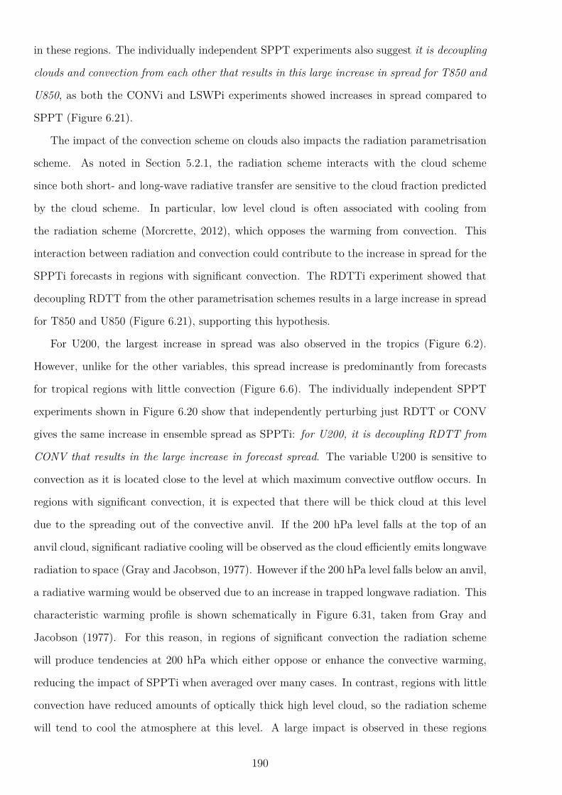
in these regions. The individually independent SPPT experiments also suggest it is decoupling
clouds and convection from each other that results in this large increase in spread for T850 and
U850, as both the CONVi and LSWPi experiments showed increases in spread compared to
SPPT (Figure 6.21).
The impact of the convection scheme on clouds also impacts the radiation parametrisation
scheme. As noted in Section 5.2.1, the radiation scheme interacts with the cloud scheme
since both short- and long-wave radiative transfer are sensitive to the cloud fraction predicted
by the cloud scheme. In particular, low level cloud is often associated with cooling from
the radiation scheme (Morcrette, 2012), which opposes the warming from convection. This
interaction between radiation and convection could contribute to the increase in spread for the
SPPTi forecasts in regions with significant convection. The RDTTi experiment showed that
decoupling RDTT from the other parametrisation schemes results in a large increase in spread
for T850 and U850 (Figure 6.21), supporting this hypothesis.
For U200, the largest increase in spread was also observed in the tropics (Figure 6.2).
However, unlike for the other variables, this spread increase is predominantly from forecasts
for tropical regions with little convection (Figure 6.6). The individually independent SPPT
experiments shown in Figure 6.20 show that independently perturbing just RDTT or CONV
gives the same increase in ensemble spread as SPPTi: for U200, it is decoupling RDTT from
CONV that results in the large increase in forecast spread. The variable U200 is sensitive to
convection as it is located close to the level at which maximum convective outflow occurs. In
regions with significant convection, it is expected that there will be thick cloud at this level
due to the spreading out of the convective anvil. If the 200 hPa level falls at the top of an
anvil cloud, significant radiative cooling will be observed as the cloud efficiently emits longwave
radiation to space (Gray and Jacobson, 1977). However if the 200 hPa level falls below an anvil,
a radiative warming would be observed due to an increase in trapped longwave radiation. This
characteristic warming profile is shown schematically in Figure 6.31, taken from Gray and
Jacobson (1977). For this reason, in regions of significant convection the radiation scheme
will produce tendencies at 200 hPa which either oppose or enhance the convective warming,
reducing the impact of SPPTi when averaged over many cases. In contrast, regions with little
convection have reduced amounts of optically thick high level cloud, so the radiation scheme
will tend to cool the atmosphere at this level. A large impact is observed in these regions
190
Figure 6.31: Typical radiation induced temperature changes in the tropics for a clear skyregion compared to a ‘disturbance’ region with thick high cloud cover. Taken from Gray andJacobson (1977).
when the opposing CONV and RDTT tendencies are decoupled using SPPTi. Decoupling the
convective and radiative temperature tendencies affects the horizontal temperature gradients
at 200 hPa, which could then affect the zonal wind speed at that level1.
Considering the YOTC tendencies at 200 hPa provides support for this hypothesised mech-
anism. Figure 6.32 shows the 24 hr temperature tendencies of RDTT, CONV and LSWP at
200 hPa, averaged over 30 start dates between 14 April and 6 September 2009. Each scattered
point represents the tendency from two schemes at a particular location. Figure (a) shows that
in regions of significant convection, while the temperature tendencies are consistently positive,
radiation tendencies can be either positive or negative. In regions with little convection, the
convective tendencies remain positive on average, but the radiative tendencies are negative on
average.
The impact of SPPTi on U200 could also be indicative of an improved variability of con-
vection in the IFS. The upper level wind field is sensitive to waves generated remotely by
convective systems (Stensrud, 2013). The improvement in ensemble spread and reduction in
error is most apparent at a lead time of ten days (Figure 6.8), which could suggest that this
improvement is due to a remote source. Other diagnostics indicate that convection is better
represented when SPPTi is used instead of SPPT. The skill of convective precipitation forecasts
at T159 improve at all lead times when SPPTi is used; forecasts show an improved ensemble
spread and a slight reduction in RMSE, though the wet bias of the model is also increased.
Forecasts of TCWV show a significant improvement when SPPTi is used. The bias is reduced,
1The RDTT parametrisation scheme directly affects the atmospheric temperature only, so the observedimpact of RDTTi on U indicates a feedback mechanism
191

−5 0 5
−2
0
2
∆ T (CONV)∆
T (
RD
TT
)
(a)
−2 0 2 4−2
0
2
∆ T (LSWP)
∆ T
(R
DT
T)
(b)
−5 0 5
−2
0
2
4
∆ T (CONV)
∆ T
(LS
WP
)(c)
Figure 6.32: The 24-hour cumulative temperature tendencies at 200 hPa taken from the YOTCdata set for the RDTT, CONV and LSWP parametrisation schemes. The tendencies havebeen averaged over 30 dates between 14 April and 6 September 2009, with subsequent startdates separated by five days. The scattered points represent pairs of parametrised tendenciesfrom different spatial locations sampled over: the entire globe (grey); regions with significantconvection (red); regions with little convection (blue). The regions are those defined in Section5.5.1. Figure (a) compares the RDTT and CONV tendencies; (b) compares the RDTT andLSWP tendencies; (c) compares the LSWP and CONV tendencies.
and the spread of the forecasts improves significantly.
The increase in ensemble spread is certainly beneficial. However, is it physically reasonable
to decouple the parametrisation schemes in this way? As described in Section 5.2.1, the IFS
calls the parametrisation schemes sequentially to ensure balance between the different physics
schemes. Additionally, the different schemes in the IFS have been tuned to each other, possibly
with compensating errors. An increase of forecast error could be expected on decoupling the
schemes. This is indeed the case when SPPTi is implemented, and an increase in forecast bias
is observed for many variables. Maintaining balance is particularly important for the cloud
and convection parametrisation schemes as they represent two halves of the same process,
and because the division of labour between the two schemes is primarily dependent on model
resolution (ECMWF, 2012). The convection scheme is in balance with the cloud scheme:
the net deterministic tendency for the two schemes is close to zero. It is plausible that the
increase in RMSE in the SPPTi, CONVi and LSWPi experiments, most noticeably for T850
and Z500, could be attributed to the decoupling of the cloud and convection schemes, which
could remove this balance. At T159, the increase in RMSE for T850 only occurs for predictable
forecast situations with small forecast spread. It is possible that the CONV and LSWP schemes
192

have been tuned to be very accurate for these specific cases, so decoupling the two schemes
by introducing SPPTi has a detrimental effect on the forecast accuracy. This explanation is
supported by the results of the CONVi experiment — the RMS error-spread diagnostic for this
experiment had an upward ‘hook’ at small spreads, indicating a significant increase in error
for previously accurate forecast situations. At T639, Figure 6.28(a) indicates that the increase
in RMSE for T850 forecasts occurs uniformly across forecast cases. It is interesting that the
high resolution model behaves differently to the low resolution model, but further experiments
are required to diagnose the cause.
Despite the increase in forecast error, SPPTi clearly has some merit. It skilfully increases
the ensemble spread in under-dispersive regions, which tend to be those with significant convec-
tion. The resultant ensemble spread evolves in a very similar way to the RMSE — the scheme
appears to represent the uncertainty in the forecast very accurately. In the extra-tropics,
forecasts remain well calibrated and SPPTi has little effect. Hermanson (2006) considers the
difference between parametrised IFS tendencies at T799 and at T95, using the T799 integration
as a proxy for “truth”. He calculates a histogram for the sum of the temperature tendencies
from clouds and convection for each model. Both peaks were centred at between -1 and 0K/day.
However, the T95 model was observed to have a narrower, taller peak in the histogram than
the T799 model. This indicates that the lower resolution version of the IFS is underestimating
the variability of the sum of the cloud and convective tendencies — the low resolution model is
too balanced. It would be interesting to perform similar experiments using the current model
to test this balance hypothesis. If it is the case that the convection and cloud schemes are
too balanced, this could justify the use of SPPTi, and explain the source of the increased
skill, especially for the convection diagnostics. It would also be interesting to perform further
experiments using SPPTi — it is possible that using a common base pattern for the CONV
and LSWP perturbations and applying independent patterns to a smaller degree would be
beneficial, retaining a large degree of the balance between convection and clouds, but allowing
ensemble members to explore the slightly off-balance scenarios observed by Hermanson (2006)
in the higher resolution model.
The RDTTi experiment also merits further investigation as it resulted in a significant im-
provement in ensemble spread when tested at T159, but with no associated increase in RMSE.
In fact, RDDTi resulted in a reduction of error for U200 in regions with little convection, which
193

is also observed for forecasts using SPPTi in this region — the bias for U200 is reduced in re-
gions with little convection. The reduction in RMSE indicates that the stochastic perturbations
to CONV and RDTT should be uncorrelated. The radiation scheme is affected by the convec-
tion scheme through the cloud parametrisation. However, this coupling between radiation and
clouds is through a Monte-Carlo calculation (the McICA scheme), so unless the cloud fractions
are systematically wrong, the correlation between the error from the cloud scheme and the
error from the radiation scheme should be reduced. The independent pattern approach could
therefore be a physically reasonable model for the errors between the convection and radiation
tendencies. It would be interesting to test the RDTTi scheme at T639 to see if a reduction in
RMSE is observed and if the forecast skill is improved at operational resolution.
In conclusion, modifying the SPPT scheme to allow independent perturbations to the para-
metrised tendencies has a significant positive impact on the spread of the ensemble forecasts
at T159 resolution. The improvement in ensemble spread was also observed at T639, though
this was accompanied by an increase in RMSE for some variables. Nevertheless, ECMWF is
very interested in performing further experiments using the SPPTi scheme to test its potential
for use in the operational EPS.
194

7
Conclusion
It seems to me that the condition of confidence or otherwise forms a very important
part of the prediction, and ought to find expression. It is not fair to the forecaster that
equal weight be assigned to all his predictions and the usual method tends to retard
that public confidence which all practical meteorologists desire to foster.
– W. Ernest Cooke, 1906
Reliability is a necessary property of forecasts for them to be useful to decision makers for
risk assessment, as described in Chapter 1 (Zhu et al., 2002). In order to produce reliable prob-
abilistic weather forecasts, it is important to account for all sources of error in atmospheric
models. In the case of weather prediction, the two main sources of error arise from initial
condition uncertainty and model uncertainty (Slingo and Palmer, 2011). There has been much
interest in recent years in using stochastic parametrisations to represent model uncertainty
in atmospheric models (Buizza et al., 1999; Lin and Neelin, 2002; Craig and Cohen, 2006;
Khouider and Majda, 2006; Palmer et al., 2009; Bengtsson et al., 2013). Stochastic paramet-
risations have been shown to correct under-dispersive ensemble spread and improve the overall
skill of the forecasts. However, there has been little research in explicitly testing the skill of
stochastic parametrisations at representing model uncertainty — existing stochastic schemes
have been tested in situations where there is also initial condition uncertainty, so it is hard
to determine to what degree the representation of initial condition uncertainty accounts for
model uncertainty, and vice versa. Additionally, there has been little research into the impact
of stochastic schemes on climate prediction. However, research into the ‘seamless prediction’
paradigm states that in order to predict the climate skilfully, a model should be skilful at
195

predicting shorter time scale events. This ansatz can be used to evaluate and improve climate
models (Rodwell and Palmer, 2007; Palmer et al., 2008; Martin et al., 2010).
This study has tested stochastic parametrisations for their ability to represent model un-
certainty skilfully in atmospheric models, and thereby to produce reliable, flow-dependent
probabilistic forecasts. The main aims were:
1. To explicitly test stochastic parametrisations as a way of representing model uncertainty
in atmospheric models. An idealised set up in the Lorenz’96 system allows the initial
conditions to be known exactly, leaving model uncertainty as the only source of error in
the forecast.
2. To test stochastic parametrisations for their ability to simulate the climate of a model.
Is it true that, following the seamless prediction paradigm, a model which is unreliable
in predicting the weather is likely to be unreliable in predicting the climate?
For both of these, the skill of stochastic parametrisation schemes is compared to perturbed
parameter schemes. These are commonly used as deterministic representations of uncertainty
in climate models. The final aim is:
3. To use the lessons learned in a simple system to test and develop stochastic and per-
turbed parameter representations of model uncertainty for use in an operational weather
forecasting model.
The main findings of this thesis are summarised below.
Stochastic parametrisations are a skilful way of representing model uncertainty in
weather forecasts.
It is important to represent model uncertainty in weather forecasts: the forecasts in the L96
system, described in Chapter 2, showed a significant improvement in skill when a represent-
ation of model uncertainty was included in the forecast model compared to the deterministic
forecasts. The stochastic parametrisation schemes produced the most skilful forecasts. More
importantly, the best stochastic parametrisation scheme, using multiplicative AR(1) noise, was
shown to be reliable, i.e., the ensemble was able to capture the uncertainty in the forecast due
to limitations in the forecast model. This indicates that stochastic parametrisations are a
skilful approach for representing model uncertainty in weather forecasts.
196
Using the L96 system to test stochastic parametrisations was advantageous because it
allowed initial condition uncertainty to be removed, leaving only model uncertainty. This is not
the case for the experiments using the IFS. Nevertheless, the new independent SPPT scheme
presented in Chapter 6 seems to be a skilful way of representing model uncertainty in the IFS,
improving the reliability of the ensemble forecasts, though resulting in too much spread for
some variables. However, the results at T639 indicate that initial condition perturbations are
routinely over-inflated to correct for the lack of spread generated by the operational stochastic
parametrisation schemes. The proposed SPPTi scheme could make inflation of initial condition
perturbations unnecessary in the IFS.
The perturbed parameter ensemble forecasts tested in the L96 system were more skilful
than a single deterministic forecast with no representation of model uncertainty, but they
were not as skilful as the best stochastic schemes (Chapter 2). This is despite estimating the
degree of parameter perturbation from the truth time series. The same result was obtained in
Chapter 5 when perturbed parameter ensembles were tested in the IFS — a relatively small
impact on forecast skill was observed, despite estimating the uncertainty in the parameters
using a Bayesian approach. This indicates that parameter uncertainty is not the only source
of model uncertainty in atmospheric models. In fact, assumptions and approximations made
when constructing the parametrisation scheme also result in errors which cannot be represented
by varying uncertain parameters. The stochastically perturbed parameter scheme tested in
the IFS also had a small positive impact on skill. However, the temporal and spatial noise
correlations were not estimated or tuned for this scheme, and the standard SPPT values were
used instead. It is likely that the optimal noise parameters would be different for a perturbed
parameter scheme than for SPPT, and using measured noise parameters could result in further
improvement in the forecast skill.
It is important to represent short time-scale model uncertainty in climate forecasts.
Stochastic parametrisations are a skilful way of doing this.
In Chapter 3, the L96 forecast model climatology showed a significant improvement over the
deterministic forecast model when stochastic parametrisations were used to represent model
uncertainty. The climate pdf simulated by the stochastic models was a better estimate of the
truth pdf than that simulated by the deterministic model. The improvement in climatology
197

was particularly clear when considering the regime behaviour of the L96 system. The determ-
inistic forecast was unable to explore both regimes, and did not capture the variability of the
‘truth’ model. The stochastic forecast model performed significantly better, and was able to
capture both the proportion of time spent in each regime, and the regime transition time scales.
Studying the regime behaviour of a system provides much more information than comparing
the pdfs: this verification technique should be used when testing climate models.
The perturbed parameter ensembles were also tested on their ability to simulate the climate
of the L96 system. As each ensemble member is a physically distinct model of the system,
ensemble members should be treated independently. The average perturbed parameter pdf is
significantly more skilful than the deterministic pdf, though less skilful than the best stochastic
schemes. Each individual ensemble member also produces a skilful pdf. The perturbed para-
meter model was tested on its ability to simulate regime behaviour in the L96 system. While
the average of the ensemble members performed well, individual ensemble members varied
widely. Many performed very poorly and only explored one regime. A similar result was ob-
served in the IFS in Chapter 5, when forecasts with the perturbed parameter ensemble were
considered. Over the ten day forecast time window, significant trends in tropical total column
water vapour were observed, with some ensemble members systematically drying and others
systematically moistening. Over a climate length integration, it is possible that these biases
would continue to grow. The stochastically perturbed parameter ensemble did not develop
these biases, so this could be a better way of representing parameter uncertainty in climate
models.
The results presented provide some support for the ‘seamless prediction’ paradigm: the
climatological skill of the forecast models was related to their skill at predicting the weather.
The results suggest that it is a necessary but not sufficient condition that a skilful climate
model produce reliable short range forecasts.
Skilful stochastic parametrisations should have a realistic representation of the
model error
In Chapters 2 and 3, a significant improvement in weather and climate forecast skill for the
L96 system was observed when the stochastic parametrisation schemes included temporally
correlated (red) noise. This more accurately reflects the true sub-grid scale forcing from the
198

Y variables, which shows high temporal autocorrelation. In the atmosphere, it is likely that
the error in the sub-grid scale tendency (the difference between the parametrised and true
tendencies) also has a high degree of temporal and spatial correlation, which a stochastic
parametrisation scheme should represent.
In the L96 system, the more realistic c = 4 case further demonstrates the importance
of realistically representing noise in a stochastic parametrisation scheme: the more accurate
stochastic representations of the sub-grid scale forcing (the SD, M and MA schemes — see
Chapter 2 for more details) produced significantly more skilful weather forecasts than the
simple additive noise case. This is also the case for both the pdf and regime definitions of
climate considered.
In the IFS, it is not realistic to assume that the errors arising from different parametrisation
schemes are perfectly correlated, and relaxing this assumption in Chapter 6 was found to result
in a significant improvement in forecast reliability. However, it is unlikely that the errors
from different parametrisation schemes are completely uncorrelated, so measuring the degree
of correlation would be an important step for producing a realistic representation of model
uncertainty in the IFS.
Stochastic ensemble forecasts contain information about flow-dependent model
uncertainty, which is absent from statistically generated ensembles.
A new proper score, the Error-spread Score (ES), was proposed in Chapter 4, suitable for evalu-
ation of ensemble forecasts. The score is particularly sensitive to the dynamic (flow-dependent)
reliability of ensemble forecasts, and detects a large improvement in skill for ensemble forecasts
compared to a statistically generated ‘dressed deterministic’ forecast. The decomposition of
the score indicates that the stochastic EPS forecasts have improved reliability over much of
the tropics compared to a statistical approach, and also have an improved resolution. The
ES detects skill in probabilistic seasonal forecasts of sea surface temperature in the Nino 3.4
region compared to both climatological and persistence forecasts.
The skill of ensemble forecasts at predicting flow-dependent uncertainty is also reflected
in an improved RMS error-spread scatter plot: the forecast model can distinguish between
predictable and unpredictable days, and correctly predicts the error in the ensemble mean.
The stochastic parametrisations tested in the L96 system (Chapter 2), and the SPPTi scheme
199

tested in the IFS (Chapter 6) both showed improvements using this diagnostic.
Limitations of Work and Future Research
It is important to consider the limitations of this study when drawing conclusions. These
limitations also suggest interesting or constructive research projects which could extend the
work presented in this thesis.
The L96 model was designed to be a simple model of the atmosphere, with desirable prop-
erties including fully chaotic behaviour and interaction between variables of different scales.
However, it is a very simple model, and so has limitations. It is only possible to test statist-
ically derived parametrisation schemes in the context of this model as opposed to those with
a more physical basis. This is true for both the deterministic and stochastic parametrisation
schemes analysed in this study. Nevertheless, the L96 system has many benefits. It allows
idealised experiments to be carried out, in which initial condition uncertainty can be removed.
It is also cheap to run, which allows the generation of a very large truth data set, so that the
parameters in the deterministic and stochastic schemes can be accurately determined. It also
allows large forecast-verification data sets and very long climate runs to be produced, giving
statistically significant results.
In Chapter 3, the L96 model was shown to have two distinct regimes, similar to regimes
observed in the atmosphere. However, in the L96 system, one regime is much weaker than
the other, and describes only 20% of the time series. This is dissimilar to what is observed
in the atmosphere. For example, four distinct weather regimes are observed in the North
Atlantic in winter, each accounting for between 21.0%−29.2% of the time series — a relatively
even split between the four regimes (Dawson et al., 2012). Nevertheless, the weaker regime in
the L96 system is sufficiently robust to appear in several diagnostics, for both the smoothed
and unsmoothed time series, and the different representations of model uncertainty tested in
this study had a noticeable impact on simulating the regime behaviour. It would be very
interesting to further this work by considering atmospheric models. Recent work indicates
that stochastic parametrisations can improve the representation of regimes in the IFS (Andrew
Dawson, pers. comm., 2013), but there has been no work considering the representation of
regimes by perturbed parameter ensembles. We have carried out preliminary experiments
testing the regime behaviour of the climateprediction.net ‘Weather at Home’ data set, which
200
looks like an interesting route for further investigation.
The proposed ES is an attractive score as it uses the raw ensemble output to verify the
forecasts, and it is suitable for continuous forecasts. It is also sensitive to the ‘dynamic re-
liability’ of the forecast, which other scores seem insensitive to. However, it is only suitable
for ensemble forecasts with a sufficiently large number of members. This is because of the
need to calculate the third order moment of the ensemble, which is particularly sensitive to
sampling errors. Poor estimates of the ensemble skewness can result in erroneously large values
of the score. The ES decomposition provides useful information about the source of skill in the
forecast, as well as aiding an understanding of how the score works. However, this requires a
very large forecast-verification sample because of the need to bin the forecast-verification pairs
in two dimensions. This makes it unsuitable for small or preliminary studies where only a few
dates may be tested. Nevertheless, ECMWF have expressed an interest in including the ES
in their operational verification suite, which I will implement over the next few months. This
will provide a very large data set which I can use to test the score further, which should help
provide a more complete understanding of the score’s strengths and weaknesses.
In Chapter 5, precipitation is an important variable to consider for verification. It is pro-
duced by the convection scheme, so studying precipitation should detect improvements in the
parametrisation of convection. However, verification of precipitation is difficult as measure-
ments of precipitation are not assimilated into the IFS using the 4DVar or EDA systems. In
Chapter 5, the GPCP data set was used for verification which includes information from both
satellites and rain gauges. This data set is likely to contain errors, particularly in small scale
features, which have not been accounted for when verifying the IFS forecasts. It is likely that
the regridding process (from a one-degree to a T159 reduced Gaussian grid) introduces addi-
tional errors. Spatially averaging the GPCP and forecast fields before verification, e.g. to a
T95 grid, should reduce this error, and will be considered in future work.
The main limitation of the experiments carried out in the IFS stem from the low resolution
of the forecasts. Using a resolution of T159 is computationally affordable, but has a grid point
spacing four times larger than the operational T639 resolution. While the T639 forecasts in
Chapter 6 showed similar trends to the T159 forecasts, it is apparent that the operational T639
forecasts are better calibrated than the T159 forecasts. This makes it hard to analyse the T159
forecasts, which are significantly under-dispersive, and which amplify the need to increase the
201

forecast spread in the tropics. At T159, the SPPTi scheme results in a well calibrated ensemble,
while at T639, it results in a significantly over-dispersive ensemble forecast for some variables.
Future research will focus on repeating experiments of interest at operational resolution. In
particular, it will be interesting to test the RDDTi scheme, as well as testing a common base
pattern for the CONV and LSWP tendencies. Additionally, it will be interesting to consider
ensemble forecasts using a reduced initial condition perturbation, specifically, we propose to
use the raw EDA output to provide the initial condition perturbations. This could be a
more realistic representation of initial condition uncertainty, and could improve the spread-
error relationship when used in conjunction with SPPTi. This work is already scheduled to
be done in collaboration with ECWMF. The ultimate aim is to improve the SPPTi scheme,
reducing the forecast RMSE while maintaining the improvement in reliability, such that it can
be incorporated into a future cycle of the IFS.
The results from the L96 system motivate the importance of including accurate spatial
and temporal correlations in a stochastic parametrisation scheme. However, this correlation
structure has never been studied in a weather forecasting model, and an arbitrary structure is
currently imposed in the SPPT scheme. An interesting research direction will be to use coarse
graining experiments to physically derive this correlation structure, before implementing it in
the ECMWF model. This could significantly increase the skill of the forecast, while increasing
our understanding of the limitations of parametrisation schemes.
The key assumption in the formulation of SPPT is that one can treat uncertainty from
each parametrisation scheme in the same way. In contrast, the SPPTi scheme assumes that
the different parametrisation schemes have independent errors, but that multiplicative noise
is still a good approach. There has been no research, to my knowledge, which addresses the
interaction of uncertainties from different physics schemes, yet it is particularly important that
this is understood if a move is made away from schemes such as SPPT which represent overall
uncertainty, to using different representations for different schemes. To address this, I propose
to use a series of coarse graining experiments, which use high resolution simulations (where,
to a large extent, parametrisation schemes are not required) to evaluate how the uncertainties
from each parametrisation scheme interact, and how SPPT and/or SPPTi should be adapted
if uncertainties from different parametrisation schemes must be treated independently.
Finally, the results from the L96 system indicate that stochastic parametrisations could
202

be a powerful tool for improving a model’s climatology. It would be useful to perform ex-
periments which could provide further proof whether stochastic parametrisation in climate
models is a direction worth pursuing. Firstly, it would be interesting to carry out a series
of experiments using the ECMWF model at longer lead times of one month. At these time
scales, initial condition uncertainty becomes less important, and the climatology of the fore-
cast model becomes significant. The seamless prediction paradigm proposes that the skill of
the stochastic and perturbed parameter schemes at monthly time scales is linked to their skill
at weekly time scales: these experiments would test this hypothesis. Furthermore, perturbed
parameter experiments have traditionally been used in climate prediction, whereas stochastic
parametrisations have remained confined to weather forecasts. The consideration of monthly
forecasts, where validation is possible, will indicate which scheme could produce the most re-
liable estimates of anthropogenic climate change, which cannot otherwise be tested. I would
then move on to apply the insights gained from these experiments to seasonal forecasting. Ac-
curate representation of model uncertainty is crucial at seasonal time scales, and the reliability
of seasonal forecasts can be tested through comparison with observations. Because of this,
seasonal forecasts provide an excellent way of testing stochastic parametrisations before they
are implemented in climate models.
The results presented in this study indicate that stochastic parametrisations are a skil-
ful approach to representing model uncertainty in atmospheric simulators. The reliability
of weather forecasts can be improved by using stochastic parametrisation schemes, provided
these schemes are designed to represent the model error accurately, for example, by using
spatially and temporally correlated noise. Furthermore, stochastic schemes have the potential
to improve a model’s climatology; testing and development of stochastic parametrisations in
climate models should be an important focus for future research. With further development of
physically-based stochastic parametrisation schemes, we could have the potential to produce
the reliable, flow-dependent, probabilistic forecasts required by users for decision making.
203

204

Appendix A
Skill Score Significance Testing
A.1 Weather Forecasts in the Lorenz ‘96 System
In order to state with confidence that one parametrisation is better than another, it is necessary
to know how significantly different one skill score is from another. The simple Monte-Carlo
technique used here evaluates how significant the difference is between two skill scores, assuming
the null hypothesis that the two parametrisations have equal skill.
Take the situation when the significance of the difference between two Skill Scores (SS)
must be evaluated. Consider two vectors, A and B, which contain the values of the skill score
evaluated for each forecast-verification pair for forecast models A and B respectively. The skill
score for the forecast model is the average of these individual scores. The vectors are each of
length n, corresponding to the number of forecast-verification pairs considered.
If the forecasts have equal skill, the elements of A and B are interchangeable, and any
apparent difference in skill of forecast system A over B is due to chance. Therefore, the
elements of A and B were pairwise shuffled 4000 times, and the skill of the shuffled vector
forecasts calculated. The difference in skill score, D = SS(A) − SS(B) is calculated, and
the probability of occurrence of the measured D assuming the null hypothesis is evaluated.
The significance of the difference between the skill of the forecast models tested in the L96
system is calculated following the method above. The details of the different models, and the
skill of the models at short term forecasts in the L96 system are presented in Chapter 2.
The following tables contain the proportion of shuffled forecast skill scores with a smaller
difference, D, than that measured (to two decimal places). For the RPSS and IGNSS, if the
proportion is greater than 0.95, andDmeas is positive, forecast A is considered to be significantly
205

W A AR1 A W SD AR1 SD W M AR1 M W MA AR1 MA PPDet. 1.00 1.00 1.00 1.00 1.00 1.00 1.00 1.00 1.00W A ⋆ 1.00 0.00 1.00 0.94 1.00 0.56 1.00 1.00AR1 A ⋆ 0.00 1.00 0.00 1.00 0.00 1.00 0.00W SD ⋆ 1.00 1.00 1.00 1.00 1.00 1.00AR1 SD ⋆ 0.00 1.00 0.00 0.95 0.00W M ⋆ 1.00 0.07 1.00 1.00AR1 M ⋆ 0.00 0.00 0.00W MA ⋆ 1.00 1.00AR1 MA ⋆ 0.00
Table A.1: Significance values for improvement of [column heading] parametrisation (C) over[row heading] parametrisation (R), calculated for the RPSS for the c = 4 case. Blue indicatesC is significantly more skilful than R at the 95% significance level, while red indicates R issignificantly more skilful than C.
W A AR1 A W SD AR1 SD W M AR1 M W MA AR1 MA PPDet. 1.00 1.00 1.00 1.00 1.00 1.00 1.00 1.00 1.00W A ⋆ 1.00 0.00 1.00 1.00 1.00 0.07 1.00 1.00AR1 A ⋆ 0.00 0.88 0.00 1.00 0.00 0.88 0.12W SD ⋆ 1.00 1.00 1.00 0.97 1.00 1.00AR1 SD ⋆ 0.00 0.98 0.00 0.55 0.04W M ⋆ 1.00 0.00 1.00 1.00AR1 M ⋆ 0.00 0.03 0.00W MA ⋆ 1.00 1.00AR1 MA ⋆ 0.03
Table A.2: As for Table A.1, except the significance of difference in RPSS for the c = 10 case.
more skilful than forecast B (at the 95% level), and is coloured blue in Tables A.1–A.4. If the
proportion is less than 0.05, and Dmeas is negative, forecast A is considered to be significantly
worse than forecast B, and is coloured red.
For REL a smaller value indicates improved reliability. Therefore if the proportion is less
than 0.05, and Dmeas is negative, forecast A is considered to be significantly more skilful than
forecast B (at the 95% level), and is coloured blue in Tables A.5–A.6. If the proportion is
greater than 0.95, and Dmeas is positive, forecast A is considered to be significantly worse than
forecast B, and is coloured red.
A.2 Simulated Climate in the Lorenz ‘96 System
The significance of the difference between two climatological pdfs is calculated using a similar
Monte-Carlo technique. The details of the forecast models are presented in Chapter 2, and
206
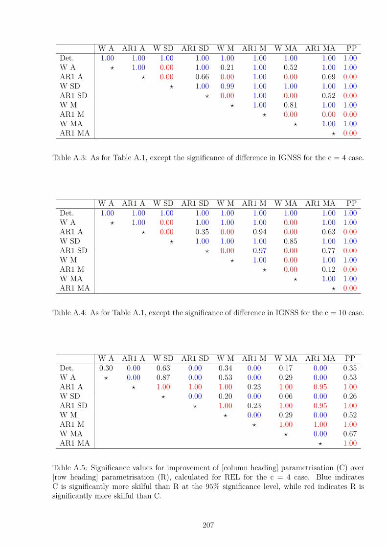
W A AR1 A W SD AR1 SD W M AR1 M W MA AR1 MA PPDet. 1.00 1.00 1.00 1.00 1.00 1.00 1.00 1.00 1.00W A ⋆ 1.00 0.00 1.00 0.21 1.00 0.52 1.00 1.00AR1 A ⋆ 0.00 0.66 0.00 1.00 0.00 0.69 0.00W SD ⋆ 1.00 0.99 1.00 1.00 1.00 1.00AR1 SD ⋆ 0.00 1.00 0.00 0.52 0.00W M ⋆ 1.00 0.81 1.00 1.00AR1 M ⋆ 0.00 0.00 0.00W MA ⋆ 1.00 1.00AR1 MA ⋆ 0.00
Table A.3: As for Table A.1, except the significance of difference in IGNSS for the c = 4 case.
W A AR1 A W SD AR1 SD W M AR1 M W MA AR1 MA PPDet. 1.00 1.00 1.00 1.00 1.00 1.00 1.00 1.00 1.00W A ⋆ 1.00 0.00 1.00 1.00 1.00 0.00 1.00 1.00AR1 A ⋆ 0.00 0.35 0.00 0.94 0.00 0.63 0.00W SD ⋆ 1.00 1.00 1.00 0.85 1.00 1.00AR1 SD ⋆ 0.00 0.97 0.00 0.77 0.00W M ⋆ 1.00 0.00 1.00 1.00AR1 M ⋆ 0.00 0.12 0.00W MA ⋆ 1.00 1.00AR1 MA ⋆ 0.00
Table A.4: As for Table A.1, except the significance of difference in IGNSS for the c = 10 case.
W A AR1 A W SD AR1 SD W M AR1 M W MA AR1 MA PPDet. 0.30 0.00 0.63 0.00 0.34 0.00 0.17 0.00 0.35W A ⋆ 0.00 0.87 0.00 0.53 0.00 0.29 0.00 0.53AR1 A ⋆ 1.00 1.00 1.00 0.23 1.00 0.95 1.00W SD ⋆ 0.00 0.20 0.00 0.06 0.00 0.26AR1 SD ⋆ 1.00 0.23 1.00 0.95 1.00W M ⋆ 0.00 0.29 0.00 0.52AR1 M ⋆ 1.00 1.00 1.00W MA ⋆ 0.00 0.67AR1 MA ⋆ 1.00
Table A.5: Significance values for improvement of [column heading] parametrisation (C) over[row heading] parametrisation (R), calculated for REL for the c = 4 case. Blue indicatesC is significantly more skilful than R at the 95% significance level, while red indicates R issignificantly more skilful than C.
207

W A AR1 A W SD AR1 SD W M AR1 M W MA AR1 MA PPDet. 0.94 0.00 0.94 0.00 0.95 0.055 0.90 0.00 0.43W A ⋆ 0.00 0.33 0.00 0.51 0.00 0.28 0.00 0.04AR1 A ⋆ 1.00 1.00 1.00 0.96 1.00 0.73 1.00W SD ⋆ 0.00 0.65 0.00 0.42 0.00 0.09AR1 SD ⋆ 1.00 0.96 1.00 0.73 1.00W M ⋆ 0.00 0.27 0.00 0.03AR1 M ⋆ 1.00 0.04 0.98W MA ⋆ 0.00 0.09AR1 MA ⋆ 1.00
Table A.6: As for Table A.5, except the significance of difference in REL for the c = 10 case.
the skill of the different models at simulating the climate of the L96 system is presented in
Chapter 3.
The significance of the difference between the two climatological vectors XA and XB must
be evaluated. Each vector samples 10, 000MTU with a resolution of 0.05MTU . Firstly, each
vector is divided into sections 50MTU long. These sections are pairwise shuffled to create two
new climatological vectors, XP and XQ. The Hellinger distance between each shuffled vector
and the true climatological vector is analysed following (3.2) to give Dhell(XP) and Dhell(XQ)
respectively. The difference, D = Dhell(XP) − Dhell(XQ) is calculated. This is repeated 2000
times, and the distribution of D compared to the improvement in Hellinger distance between
the original XA and XB, Dtru = Dhell(XA) − Dhell(XB), where each Hellinger distance is
calculated by comparing to the true climatological distribution. The proportion of D smaller
than Dtru is calculated and shown in Tables A.7 and A.8.
The smaller the value of Dhell the better the simulation of the true climatology. Therefore,
if Dtru is negative, A has a better representation of the true climatology than B. In this case,
if less than 5% of the distribution of D is smaller (more negative) than Dtrue, the climate of A
is significantly better than B at the 95% significance level, and is coloured blue in Tables A.7
and A.8. Conversely, if Dtru is positive and the proportion of D smaller than Dtru is 0.95 or
greater, the climate of A is significantly worse than the climate of B, and the proportion is
coloured red in Tables A.7 and A.8.
208

W A AR1 A W SD AR1 SD W M AR1 M W MA AR1 MA PPDet. 0.34 0.00 0.26 0.00 0.40 0.00 0.56 0.00 0.00White A. ⋆ 0.00 0.39 0.00 0.56 0.00 0.70 0.00 0.00AR1 A. ⋆ 1.00 0.05 1.00 0.00 1.00 0.031 0.026White SD. ⋆ 0.00 0.67 0.00 0.79 0.00 0.00AR1 SD. ⋆ 1.00 0.005 1.00 0.39 0.26White M. ⋆ 0.00 0.65 0.00 0.00AR1 M. ⋆ 1.00 0.99 0.91White MA. ⋆ 0.00 0.00AR1 MA. ⋆ 0.32
Table A.7: Significance values for improvement of the climatology of [column heading] para-metrisation over [row heading] parametrisation, calculated for the Hellinger Distance for the c= 4 case. “0” indicates that R is better than C with a likelihood of less than 1/2000, while “1”indicates a likelihood of greater than 1999/2000. Blue indicates C is significantly more skilfulthan R at the 95% significance level, while red indicates R is significantly more skilful than C.
W A AR1 A W SD AR1 SD W M AR1 M W MA AR1 MA PPDet. 0.99 0.00 0.46 0.00 0.44 0.00 0.39 0.00 0.00White A. ⋆ 0.00 0.045 0.00 0.011 0.00 0.003 0.00 0.00AR1 A. ⋆ 1.00 0.38 1.00 0.0065 1.00 0.28 1.00White SD. ⋆ 0.00 0.47 0.00 0.42 0.00 0.00AR1 SD. ⋆ 1.00 0.013 1.00 0.39 1.00White M. ⋆ 0.00 0.45 0.00 0.0005AR1 M. ⋆ 1.00 0.96 1.00White MA. ⋆ 0.00 0.00AR1 MA. ⋆ 1.00
Table A.8: As for Table A.7, except for the c = 10 case.
209

A.3 Skill Scores for the IFS
It is necessary to calculate the significance of the difference between the skill of the different
IFS model versions to establish if a significant improvement has been made. The technique
described in Section A.1 is used. As for the L96 system, the score vectors will be pairwise
shuffled. This is because the difference between the skill of forecast system A under predict-
able flow conditions and under unpredictable flow conditions is likely to be greater than the
difference between forecast system A and B for the same conditions. It is therefore important
that each shuffled vector contains the same ratio of predictable to unpredictable cases as for
the un-shuffled cases.
When considering forecasts made using the IFS, it is important to consider spatial cor-
relations as well as temporal correlation. A time series of the thirty initial conditions was
constructed, and the spatial correlation estimated as a function of horizontal displacement
for the tropical region with significant convection. Figure A.1 shows the correlation for each
variable of interest. The time series show significant spatial correlation out to large horizontal
separations. For synoptic scales of 1,500–2,000km, the correlations are less than 0.5 for all vari-
ables, except Z500, which varies on larger spatial scales. This corresponds to a longitudinal
separation of approximately 15◦ at the equator. Therefore, to preserve the spatial correlation
in the dataset to a large degree, the skill scores for each forecast will be split into blocks
15◦ × 15◦ in size which will then be treated independently. The tropical region with significant
convection is split into sixteen blocks, for forecasts starting from 30 initial dates. There are
therefore 480 blocks of scores in total which are pairwise shuffled using the method described
in Section A.1.
A.3.1 Experiments in the IFS
The significance of the difference between the RPS is calculated for experiments using the
IFS. The results for IGN and ES are similar, so are not shown for brevity. For each figure,
each row of figures corresponds to a different variable. Each column corresponds to a different
experiment of interest. The figure shows the likelihood that the experiment of interest had
a significantly higher (poorer) score than each of the other four experiments. A likelihood
of greater than 0.95 indicates the experiment of interest is significantly worse than the other
experiment. A likelihood of less than 0.05 indicates the experiment of interest is significantly
210

0 500 1000 1500 2000 2500 3000 3500 4000
0
0.1
0.2
0.3
0.4
0.5
0.6
0.7
0.8
0.9
1
Spatial Separation / km
Cor
rela
tion
Figure A.1: Spatial correlation between initial condition time series for T850 (red), U850(green), U200 (magenta), Z500 (black), TCWV (blue) and PPT(cyan). The correlation iscalculated by the initial condition time series at some spatial separation. This was calculatedfor all points within the tropical region of significant convection defined in Figure 5.1(b) as afunction of spatial separation.
better than the other experiment. The other experiments (to which we are comparing) are
distinguished by the colour of the symbols
Figure A.2 shows the results for the stochastic and perturbed parameter experiments from
Chapter 5: TSCZ, TSCS, TSCP, TSCPr, and TSCPv.
Figure A.3 shows the results for the independent SPPT experiments from Chapter 6: TSCS,
TSCS + SKEB, TSCSi and TSCSi + SKEB.
Figure A.4 shows the results for the individually independent SPPT experiments from
Chapter 6: TSCS, TSCSi, RDDTi, TGWDi, NOGWi, CONVi, and LSWPi.
Figure A.5 shows the results for the T639 independent SPPT experiments from Chapter 6:
TSCS, TSCS + SKEB, and TSCSi.
For example: either Figure A.2 (k) or (l) can be used to ascertain the significance of the
difference between the RPS for Z500 for the TSCZ and TSCS experiments of Chapter 5. In
figure (k), the line with blue crosses indicates that TSCZ was significantly less skilful than
TSCS at short lead times, that there was no significant difference at a lead time of 120 hrs,
and that at 240 hrs, TSCZ was significantly more skilful. In figure (l), the line with black
crosses gives the same information.
211

0 100 2000
0.5
1
sign
ifica
nce
T 850
TS CZ (a)
0 100 2000
0.5
1
sign
ifica
nce
U 850
(f)
0 100 2000
0.5
1
sign
ifica
nce
Z 500
(k)
0 100 2000
0.5
1
sign
ifica
nce
U 200
(p)
0 100 2000
0.5
1
sign
ifica
nce
PPT
(u)
0 100 2000
0.5
1
lead time / hrs
sign
ifica
nce
TCWV
(z)
0 100 2000
0.5
1
TS CS (b)
0 100 2000
0.5
1(g)
0 100 2000
0.5
1(l)
0 100 2000
0.5
1(q)
0 100 2000
0.5
1(v)
0 100 2000
0.5
1
lead time / hrs
(1)
0 100 2000
0.5
1
TS CP (c)
0 100 2000
0.5
1(h)
0 100 2000
0.5
1(m)
0 100 2000
0.5
1(r)
0 100 2000
0.5
1(w)
0 100 2000
0.5
1
lead time / hrs
(2)
0 100 2000
0.5
1
TS CPr(d)
0 100 2000
0.5
1(i)
0 100 2000
0.5
1(n)
0 100 2000
0.5
1(s)
0 100 2000
0.5
1(x)
0 100 2000
0.5
1
lead time / hrs
(3)
0 100 2000
0.5
1
TS CPv(e)
0 100 2000
0.5
1(j)
0 100 2000
0.5
1(o)
0 100 2000
0.5
1(t)
0 100 2000
0.5
1(y)
0 100 2000
0.5
1
lead time / hrs
(4)
Figure A.2: Significance of difference between RPS for each pair of experiments in Chapter 5:TSCZ (black), TSCS (blue), TSCP (red), TSCPr (magenta) and TSCPv (green). Each columncorresponds to a different experiment of interest, and the four plotted lines are the significanceof the difference between that experiment and the other four, indicated by colour of markers.A value of less than 0.05 indicates the experiment of interest significantly improves on theother experiment, and a value of greater than 0.95 indicates it is significantly poorer.
212

0 100 2000
0.5
1
sign
ifica
nce
T 850
TSCS (a)
0 100 2000
0.5
1
sign
ifica
nce
U 850
(e)
0 100 2000
0.5
1
sign
ifica
nce
Z 500
(i)
0 100 2000
0.5
1
sign
ifica
nce
U 200
(m)
0 100 2000
0.5
1
sign
ifica
nce
PPT
(q)
0 100 2000
0.5
1
lead time / hrs
sign
ifica
nce
TCWV
(u)
0 100 2000
0.5
1
TSCS + SKEB (b)
0 100 2000
0.5
1(f)
0 100 2000
0.5
1(j)
0 100 2000
0.5
1(n)
0 100 2000
0.5
1(r)
0 100 2000
0.5
1
lead time / hrs
(v)
0 100 2000
0.5
1
TSCSi (c)
0 100 2000
0.5
1(g)
0 100 2000
0.5
1(k)
0 100 2000
0.5
1(o)
0 100 2000
0.5
1(s)
0 100 2000
0.5
1
lead time / hrs
(w)
0 100 2000
0.5
1
TSCSi + SKEB(d)
0 100 2000
0.5
1(h)
0 100 2000
0.5
1(l)
0 100 2000
0.5
1(p)
0 100 2000
0.5
1(t)
0 100 2000
0.5
1
lead time / hrs
(x)
Figure A.3: As for Figure A.2, except for each pair of experiments in Chapter 6: TSCS (blue),TSCS + SKEB (cyan), TSCSi (red), and TSCSi + SKEB (magenta).
213

0 100 2000
0.5
1
sign
ifica
nce
T 850
TSCS
0 100 2000
0.5
1
sign
ifica
nce
U 850
0 100 2000
0.5
1
sign
ifica
nce
Z 500
0 100 2000
0.5
1
lead time / hrs
sign
ifica
nce
U 200
0 100 2000
0.5
1
TSCSi
0 100 2000
0.5
1
0 100 2000
0.5
1
0 100 2000
0.5
1
lead time / hrs
0 100 2000
0.5
1
RDDTi
0 100 2000
0.5
1
0 100 2000
0.5
1
0 100 2000
0.5
1
lead time / hrs
0 100 2000
0.5
1
TGWDi
0 100 2000
0.5
1
0 100 2000
0.5
1
0 100 2000
0.5
1
lead time / hrs
0 100 2000
0.5
1
NOGWi
0 100 2000
0.5
1
0 100 2000
0.5
1
0 100 2000
0.5
1
lead time / hrs
0 100 2000
0.5
1
CONVi
0 100 2000
0.5
1
0 100 2000
0.5
1
0 100 2000
0.5
1
lead time / hrs
0 100 2000
0.5
1
LSWPi
0 100 2000
0.5
1
0 100 2000
0.5
1
0 100 2000
0.5
1
lead time / hrs
Figure A.4: As for Figure A.2, except for each pair of ‘individually independent’ experiments in Chapter 6: TSCS (blue), TSCSi (red), RDDTi(black), TGWDi (grey), NOGWi (yellow), CONVi (green), and LSWPi (magenta).
214
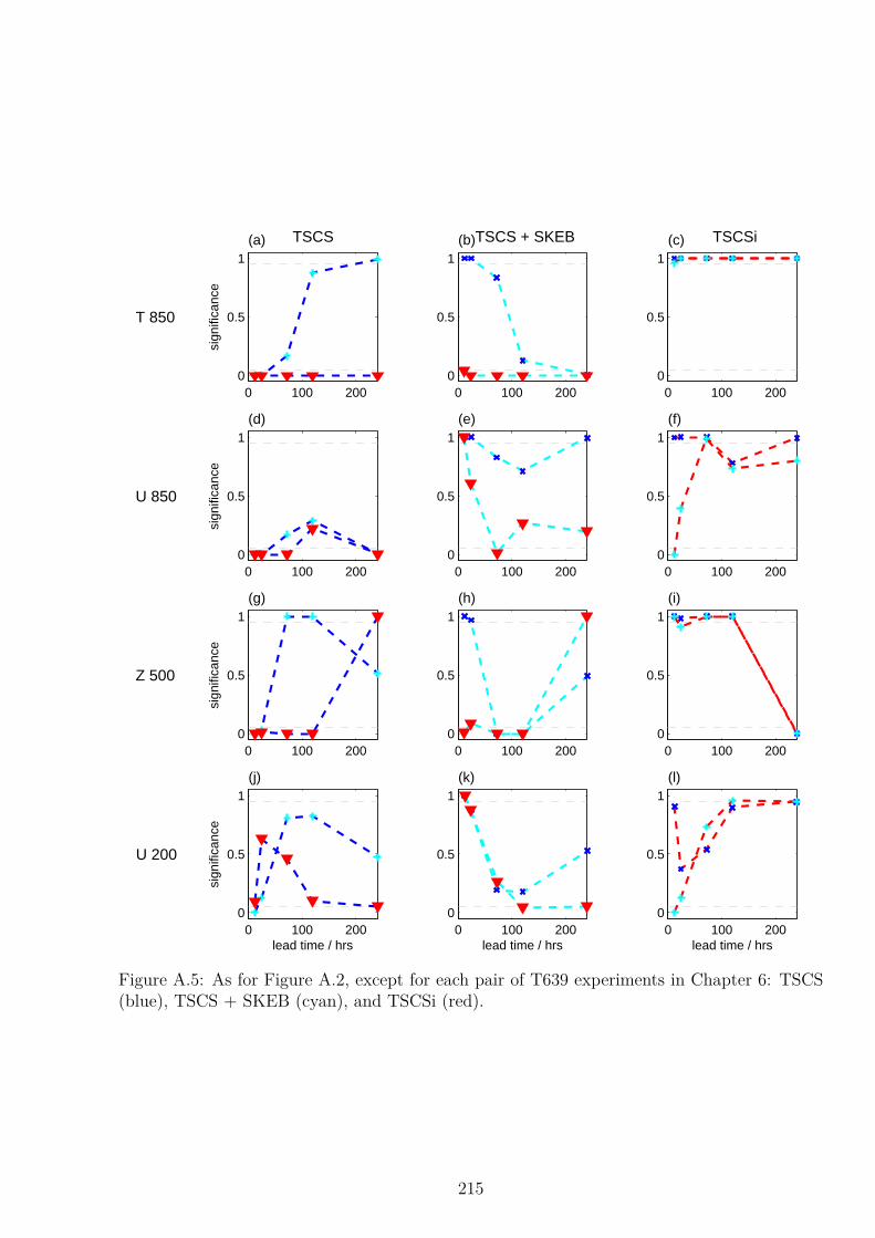
0 100 2000
0.5
1
sign
ifica
nce
T 850
TSCS (a)
0 100 2000
0.5
1
sign
ifica
nce
U 850
(d)
0 100 2000
0.5
1
sign
ifica
nce
Z 500
(g)
0 100 2000
0.5
1
lead time / hrs
sign
ifica
nce
U 200
(j)
0 100 2000
0.5
1
TSCS + SKEB(b)
0 100 2000
0.5
1(e)
0 100 2000
0.5
1(h)
0 100 2000
0.5
1
lead time / hrs
(k)
0 100 2000
0.5
1
TSCSi (c)
0 100 2000
0.5
1(f)
0 100 2000
0.5
1(i)
0 100 2000
0.5
1
lead time / hrs
(l)
Figure A.5: As for Figure A.2, except for each pair of T639 experiments in Chapter 6: TSCS(blue), TSCS + SKEB (cyan), and TSCSi (red).
215

216

Appendix B
The Error-spread Score: A Proper
Score
B.1 Derivation of the Form of the Error-Spread Score
The starting point when deriving the Error-spread Score is spread-error relationship; the ex-
pected squared error of the ensemble mean can be related to the expected ensemble vari-
ance according to (1.26) by assuming the ensemble members and the truth are independently
identically distributed random variables with variance σ2 (Leutbecher, 2010). Consider the
trial Error-spread score,
EStrial = (s2 − e2)2 (B.1)
Expanding out the brackets, and expressing the error, e, in terms of the forecast ensemble
mean, m and the verification, z:
EStrial = s4 − 2s2(m− z)2 + (m− z)4
= (s4 − 2s2m2 +m4) + z(4s2m− 4m3) + z2(4m2 − 2s2 + 2m2) − 4mz3 + z4 (B.2)
217
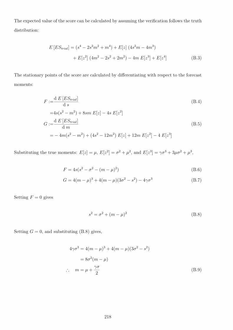
The expected value of the score can be calculated by assuming the verification follows the truth
distribution:
E [EStrial] = (s4 − 2s2m2 +m4) + E[z] (4s2m− 4m3)
+ E[z2] (4m2 − 2s2 + 2m2) − 4m E[z3] + E[z4] (B.3)
The stationary points of the score are calculated by differentiating with respect to the forecast
moments:
F :=d E [EStrial]
d s(B.4)
=4s(s2 −m2) + 8sm E[z] − 4s E[z2]
G :=d E [EStrial]
d m(B.5)
= − 4m(s2 −m2) + (4s2 − 12m2) E[z] + 12m E[z2] − 4 E[z3]
Substituting the true moments: E[z] = µ, E[z2] = σ2 + µ2, and E[z3] = γσ3 + 3µσ2 + µ3,
F = 4s(s2 − σ2 − (m− µ)2) (B.6)
G = 4(m− µ)3 + 4(m− µ)(3σ2 − s2) − 4γσ3 (B.7)
Setting F = 0 gives
s2 = σ2 + (m− µ)2 (B.8)
Setting G = 0, and substituting (B.8) gives,
4γσ3 = 4(m− µ)3 + 4(m− µ)(3σ2 − s2)
= 8σ2(m− µ)
∴ m = µ+γσ
2(B.9)
218
Substituting (B.9) into (B.8) gives,
s2 = σ2 +(
µ+γσ
2− µ
)2
= σ2
(
1 +γ2
4
)
(B.10)
Therefore, the trial Error-spread Score is not optimised if the mean and standard deviation of
the true distribution are forecast. Instead of issuing his or her true belief, (m, s), the forecaster
should predict a distribution with mean mhedged = m + gs2
and inflated standard deviation,
s2hedged = s2
(
1 + g2
4
)
in order to maximise their expected score.
To prevent a forecaster from hedging the forecast in this way, the substitution m → m+ gs2
and s2 → s2(
1 + g2
4
)
can be made in the trial Error-spread score:
EStrial :=(
s2 − (m− z)2)2
(B.11)
→ ES :=
(
s2
(
1 +g2
4
)
−(
m+gs
2− z
)2)2
ES =(s2 − e2 − esg)2 (B.12)
B.2 Confirmation of Propriety of the Error-spread Score
It is important to confirm that the Error-spread score is proper. Firstly, expand out the
brackets:
ES = (s2 − (m− z)2 − (m− z)sg)2 (B.13)
= (s2 −m2 + 2zm− z2 −msg + zsg)2
= (s4 − 2m2s2 − 2ms3g +m2s2g2 + 2m3sg +m4)
+ z(4ms2 + 2s3g − 4m2sg − 4m3 − 2ms2g2 − 2m2sg)
+ z2(−2s2 + 2m2 + 2msg + 4m2 + 4msg + s2g2)
+ z3(−4m− 2sg) + z4 (B.14)
Calculate the expectation of the score assuming the verification, z, follows the truth distri-
219
bution (equations 4.2–4.4).
E [ES] = (s4 − 2m2s2 − 2ms3g +m2s2g2 + 2m3sg +m4)
+ E [z] (4ms2 + 2s3g − 4m2sg − 4m3 − 2ms2g2 − 2m2sg)
+ E[
z2]
(−2s2 + 2m2 + 2msg + 4m2 + 4msg + s2g2)
+ E[
z3]
(−4m− 2sg) + E[
z4]
(B.15)
But
E [z] = µ, (B.16)
E[
z2]
= σ2 + µ2, (B.17)
E[
z3]
= σ3γ + 3µσ2 + µ3, (B.18)
E[
z4]
= σ4β + 4µσ3γ + 6µ2σ2 + µ4. (B.19)
Therefore
E [ES] = (s4 − 2m2s2 − 2ms3g +m2s2g2 + 2m3sg +m4)
+ µ(4ms2 + 2s3g − 4m2sg − 4m3 − 2ms2g2 − 2m2sg)
+ (σ2 + µ2)(−2s2 + 2m2 + 2msg + 4m2 + 4msg + s2g2)
+ (σ3γ + 3µσ2 + µ3)(−4m− 2sg)
+ σ4β + 4µσ3γ + 6µ2σ2 + µ4 (B.20)
Expanding and re-factorising, it can be shown that
E [ES] =(
(σ2 − s2) + (µ−m)2 − sg(µ−m))2
+ σ2 (2(µ−m) + (σγ − sg))2 + σ4(β − γ2 − 1) (B.21)
In order to be proper, the expected value of the scoring rule must be minimised when the
“truth” distribution is forecast. Let us test this here.
220

Differentiating with respect to m:
dE[ES]
dm= 2
(
(σ2 − s2) + (µ−m)2 − sg(µ−m))
(sg − 2(µ−m))
− 4σ2 (2(µ−m) + (σγ − sg)) (B.22)
= 0 at optimum.
Differentiating with respect to s:
dE[ES]
d s= 2
(
(σ2 − s2) + (µ−m)2 − sg(µ−m))
(−2s− g(µ−m))
− 2σ2g (2(µ−m) + (σγ − sg)) (B.23)
= 0 at optimum.
Differentiating with respect to g:
dE[ES]
d g= −2s(µ−m)
(
(σ2 − s2) + (µ−m)2 − sg(µ−m))
− 2σ2s (2(µ−m) + (σγ − sg)) (B.24)
= 0 at optimum.
Since d E[ES]d v
= 0 for v = m, s, g, the “truth” distribution corresponds to a stationary point of
the score. The Hessian of the score is given by
H = 2σ2
γ2 + 4 0 2σ
0 γ2 + 4 σγ
2σ σγ σ2
,
which has three eigenvalues ≥ 0. This stationary point is a minimum as required.
Additionally, a score, S is proper if, for any two probability densities P (x) and Q(x)
(Brocker, 2009),∫
S[P (x), z]Q(z) dz ≥∫
S[Q(x), z]Q(z) dz. (B.25)
where the integral is over the possible verifications, z. This criterion can be tested for the
Error-spread score. The term on the left of (B.25) is the expectation of ES calculated earlier
221

if we identify P (x) with the issued forecast and Q(x) with the “truth” distribution.
∫
S[P (x), z]Q(z) =(
(σ2 − s2) + (µ−m)2 − sg(µ−m))2
+ σ2 (2(µ−m) + (σγ − sg))2 + σ4(β − γ2 − 1) (B.26)
Similarly,
∫
S[Q(x), z]Q(z) = σ4(β − γ2 − 1) (B.27)
Therefore,
∫
S[P (x), z]Q(z) dz −∫
S[Q(x), z]Q(z)
=(
(σ2 − s2) + (µ−m)2 − sg(µ−m))2
+ σ2 (2(µ−m) + (σγ − sg))2
≥ 0 ∀ m, s and g. (B.28)
The Error-spread score is a proper score.
B.3 Decomposition of the Error-spread Score
In this decomposition, the error between the verification and the ensemble mean, (m − z), is
discussed as if it were the verification. Consider that the forecast can be transformed to centre
it on the origin, and the same transformation can be used on the verification. The statistics of
the measured error are unchanged, and will have an expected value of zero if the forecast was
unbiased, i.e. the mean of the forecast and the mean of the truth distribution are identical.
This assumption is used in the following — the error can now be thought of as the verification
as its value depends only on the measured true state of the atmosphere, assuming the forecast
ensemble mean is perfectly accurate.
Assume that the predicted spread, sk, can only take I discrete values si where i = (1, . . . , I).
Assume the predicted skewness, gk, can only take J discrete values gj where j = (1, . . . , J).
Bin the measured errors, ek, according to the predicted spread, si, and the predicted skewness,
222

gj. Defining
n =I∑
i=1
J∑
j=1
Ni,j, (B.29)
e2i,j =
1
Ni,j
∑
k∈Ni,j
e2k ≈ E[e2
k]k∈Ni,j
, (B.30)
and
e2 =1
n
n∑
k=1
e2k =
1
n
I∑
i=1
J∑
j=1
Ni,je2i,j ≈ E[e2
k], (B.31)
where n is the total number of forecast-verification pairs and Ni,j is defined as the number of
forecast-verification pairs in bin (i, j). e2i,j is the average squared error in each bin and e2 is
the climatological error, both of which represent the sample estimates of the expected value
of these errors. The binning is conditioned on the forecast spread and skew only as, for the
reasons given above, the forecast mean is unimportant if the forecast is unbiased.
The Error-Spread score can be rewritten as a sum over the IJ bins as
ES =1
n
n∑
k=1
(s2k − e2
k − ekskgk)2
=1
n
I∑
i=1
J∑
j=1
∑
k∈Ni,j
(s2i − e2
k − eksigj)2
=1
n
I∑
i=1
J∑
j=1
∑
k∈Ni,j
(s2i − e2
k)2
︸ ︷︷ ︸
A
−2eksigj(s2i − e2
k) + e2ks
2i g
2j
︸ ︷︷ ︸
B
(B.32)
Consider the first term, A, evaluating the spread of the forecast:
A =1
n
I∑
i=1
J∑
j=1
∑
k∈Ni,j
(s2i − e2
k)2 (B.33)
=1
n
I∑
i=1
J∑
j=1
Ni,j(s2i )
2 − 2s2i
∑
k∈Ni,j
e2k +
∑
k∈Ni,j
(e2k)2
.
Here it has been recognised that si is a discrete variable, constant within a bin, so can be moved
outside the summation term. Using the definitions of e2i,j and e2, the square is completed twice
223

to give:
A =1
n
I∑
i=1
J∑
j=1
Ni,j
(
s2i − e2
i,j
)2 − 1
n
I∑
i=1
J∑
j=1
Ni,j
(
e2i,j − e2
)2(B.34)
+1
n
I∑
i=1
J∑
j=1
Ni,j(e2)2 − 2Ni,je2i,j e
2 +∑
k∈Ni,j
(e2k)2
.
Recalling the definition of e2i,j, and from Eq. B.30
∑Ii=1
∑Jj=1 Ni,j(e2)2 = n(e2)2 =
∑nk=1(e
2)2,
A =1
n
I∑
i=1
J∑
j=1
Ni,j
(
s2i − e2
i,j
)2 − 1
n
I∑
i=1
J∑
j=1
Ni,j
(
e2i,j − e2
)2
+1
n
n∑
k=1
(e2)2 − 2
ne2
I∑
i=1
J∑
j=1
∑
k∈Ni,j
e2k +
1
n
I∑
i=1
J∑
j=1
∑
k∈Ni,j
(e2k)2. (B.35)
Since the ek have not been sorted according to spread and skew, the multiple summation terms
can be replaced by a summation over k:
A =1
n
I∑
i=1
J∑
j=1
Ni,j
(
s2i − e2
i,j
)2 − 1
n
I∑
i=1
J∑
j=1
Ni,j
(
e2i,j − e2
)2+
1
n
n∑
k=1
(
e2 − e2k
)2(B.36)
The first term, A, has been decomposed into a sum of squared terms.
Consider the second term, B, which evaluates the shape of the forecast. This can be written
in terms of the expectation of the moments of the error ek:
B =1
n
I∑
i=1
J∑
j=1
∑
k∈Ni,j
(
−2eksigj(s2i − e2
k) + e2ks
2i g
2j
)
=1
n
I∑
i=1
J∑
j=1
−2Ni,js3i gjE[ek]
k∈Ni,j
+ 2Ni,jsigjE[e3k]
k∈Ni,j
+Ni,js2i g
2jE[e2
k]k∈Ni,j
(B.37)
Assume E[ek]k∈Ni,j
= 0. This is equivalent to assuming there is no systematic bias in the forecast
(note that in the decomposition of A, this assumption was not required). The bias of a
forecasting system should be checked before this decomposition is applied, and the forecast
debiased if necessary. With the assumption of no bias, using Eq. B.47,
E[e3k]
k∈Ni,j
= γ
(
E[e2k]
k∈Ni,j
− (E[ek]k∈Ni,j
)2
)3/2
+ 3E[ek]k∈Ni,j
E[e2k]
k∈Ni,j
+ 2(E[ek]k∈Ni,j
)3
= γ
(
E[e2k]
k∈Ni,j
)3/2
(B.38)
224

where γ is the observed (“true”) skewness of the error distribution. Define the measured shape
factor,
Gi,j =1
Ni,j
∑
k∈Ni,j
e3k ≈ E[e3
k]k∈Ni,j
, (B.39)
which is approximately equal to the third moment of the error distribution in each bin, estim-
ated using a finite sample size. Define also the climatological shape factor,
G =1
n
I∑
i=1
J∑
j=1
Ni,jGi,j =1
n
n∑
k=1
e3k. (B.40)
From Eq. 1.26 and Eq. B.38 it can be shown that if our forecast standard deviation, si, and
skewness, gj are accurate, the measured shape factor should obey
Gi,j = −sigje2i,j. (B.41)
where the negative sign arises because the verification has a negative sign in the definition of
error, m− z, so that gj = −γ for an accurate forecast. B can be written in terms of the shape
factor, Gi,j as
B =1
n
I∑
i=1
J∑
j=1
Ni,js2i g
2j e
2i,j + 2Ni,jsigjGi,j
=1
n
I∑
i=1
J∑
j=1
Ni,j
(
sigje2i,j +Gi,j
)2
e2i,j
− 1
n
I∑
i=1
J∑
j=1
Ni,j
G2i,j
e2i,j
. (B.42)
Completing the square by adding and subtracting Ni,j
(
2Gi,jG
e2− e2
i,j
(G
e2
)2)
B =1
n
I∑
i=1
J∑
j=1
Ni,j
(
sigje2i,j +Gi,j
)2
e2i,j
− 1
n
I∑
i=1
J∑
j=1
Ni,je2i,j
Gi,j
e2i,j
− G
e2
2
+1
n
n∑
k=1
e2k
(
G
e2
)2
− 2e3k
G
e2
. (B.43)
225

Combining with Eq. B.36, the ES score can be decomposed into
ES =1
n
I∑
i=1
J∑
j=1
Ni,j
(s2i − e2
i,j)2
︸ ︷︷ ︸
a
+
(
sigje2i,j +Gi,j
)2
e2i,j
︸ ︷︷ ︸
b
− 1
n
I∑
i=1
J∑
j=1
Ni,j
(e2i,j − e2)2
︸ ︷︷ ︸
c
+ e2i,j
Gi,j
e2i,j
− G
e2
2
︸ ︷︷ ︸
d
+1
n
n∑
k=1
(e2 − e2k)2 + e2
k
(
G
e2
)2
− 2e3k
G
e2
︸ ︷︷ ︸
e
(B.44)
Term a tests the reliability of the ensemble spread, and b the reliability of the ensemble
shape. Term c tests the resolution of the predicted spread and d the resolution of the predicted
shape. The last term is the uncertainty in the forecast, which is not a function of the binning
process.
B.4 Mathematical Properties of Moments
For a random variable X which is drawn from a probability distribution, P(X), the moments
of the distribution are defined as follows. The mean, µ:
µ = E[X], (B.45)
The variance, σ2:
σ2 = E[(X − µ)2]
= E[X2] − µ2, (B.46)
The skewness, γ:
γ = E
[(X − µ
σ
)3]
=1
σ3
(
E[X3] − 3µσ2 − µ3)
, (B.47)
226

Bibliography
E. Anderson and A. Persson. User guide to ECMWF forecast products. ECMWF, Shinfield
Park, Reading, RG2 9AX, U.K., 1.1 edition, July 2013.
J. L. Anderson. The impact of dynamical constraints on the selection of initial conditions
for ensemble predictions: Low-order perfect model results. Mon. Weather Rev., 125(11):
2969–2983, 1997.
A Arakawa and W. H. Schubert. Interaction of a cumulus cloud ensemble with the large scale
environment, part I. J. Atmos. Sci., 31(3):674–701, 1974.
H. M. Arnold, I. M. Moroz, and T. N. Palmer. Stochastic parameterizations and model uncer-
tainty in the Lorenz’96 system. Phil. Trans. R. Soc. A, 371(1991), 2013.
J. V. Beck and K. J. Arnold. Parameter estimation in engineering and science. Wiley, New
York, USA, 1977.
L. Bengtsson, M. Steinheimer, P. Bechtold, and J.-F. Geleyn. A stochastic parametrization
for deep convection using cellular automata. Q. J. Roy. Meteor. Soc., 139(675):1533–1543,
2013.
J. Berner, G. J. Shutts, M. Leutbecher, and T. N. Palmer. A spectral stochastic kinetic energy
backscatter scheme and its impact on flow dependent predictability in the ECMWF ensemble
prediction system. J. Atmos. Sci., 66(3):603–626, 2009.
J. Berner, T. Jung, and T. N. Palmer. Systematic model error: The impact of increased
horizontal resolution versus improved stochastic and deterministic parameterizations. J.
Climate, 25(14):4946–4962, 2012.
N. E. Bowler, A. Arribas, K. R. Mylne, K. B. Robertson, and S. E. Beare. The MOGREPS
short-range ensemble prediction system. Q. J. Roy. Meteor. Soc., 134(632):703–722, 2008.
227

G. W. Brier. Verification of forecasts expressed in terms of probability. Mon. Weather Rev.,
78(1):1–3, 1950.
J. Brocker. Reliability, sufficiency, and the decomposition of proper scores. Q. J. Roy. Meteor.
Soc., 135(643):1512–1519, 2009.
J. Brocker, D. Engster, and U. Parlitz. Probabilistic evaluation of time series models: A
comparison of several approaches. Chaos, 19(4), 2009.
T. A. Brown. Probabilistic forecasts and reproducing scoring systems. Technical report, RAND
Corporation, Santa Monica, California, June 1970.
R. A. Bryson. The paradigm of climatology: An essay. B. Am. Meteorol. Soc., 78(3):449–455,
1997.
R. Buizza. Horizontal resolution impact on short- and long-range forecast error. Q. J. Roy.
Meteor. Soc., 136(649):1020–1035, 2010.
R. Buizza and T. N. Palmer. The singular-vector structure of the atmospheric global circula-
tion. J. Atmos. Sci., 52(9):1434–1456, 1995.
R. Buizza, M. Miller, and T. N. Palmer. Stochastic representation of model uncertainties in the
ECMWF ensemble prediction system. Q. J. Roy. Meteor. Soc., 125(560):2887–2908, 1999.
R. Buizza, M. Leutbecher, and L. Isaksen. Potential use of an ensemble of analyses in the
ecmwf ensemble prediction system. Q. J. Roy. Meteor. Soc., 134(637):2051–2066, 2008.
B. G. Cohen and G. C. Craig. Fluctuations in an equilibrium convective ensemble. part II:
Numerical experiments. J. Atmos. Sci., 63(8):2005–2015, 2006.
S. Corti, F. Molteni, and T. N. Palmer. Signature of recent climate change in frequencies of
natural atmospheric circulation regimes. Nature, 398(6730):799–802, 1999.
G. C. Craig and B. G. Cohen. Fluctuations in an equilibrium convective ensemble. part I:
Theoretical formulation. J. Atmos. Sci., 63(8):1996–2004, 2006.
D. Crommelin and E. Vanden-Eijnden. Subgrid-scale parametrisation with conditional Markov
chains. J. Atmos. Sci., 65(8):2661–2675, 2008.
228

A. Dawson, T. N. Palmer, and S. Corti. Simulating regime structures in weather and climate
prediction models. Geophys. Res. Let., 39(21):L21805, 2012.
T. DelSole. Predictability and information theory. part I: Measures of predictability. J. Atmos.
Sci., 61(20):2425–2440, 2004.
F. J. Doblas-Reyes, A. Weisheimer, N. Keenlyside, M. McVean, J. M. Murphy, P. Rogel,
D. Smith, and T. N. Palmer. Addressing model uncertainty in seasonal and annual dynamical
ensemble forecasts. Q. J. Roy. Meteor. Soc., 135(644):1538–1559, 2009.
O. Donati, G. F. Missiroli, and G. Pozzi. An experiment on electron interference. Am. J.
Phys., 41(5):639–644, 1973.
J. Dorrestijn, D. T. Crommelin, A. P. Siebesma, and H. J. J. Jonker. Stochastic parameter-
ization of shallow cumulus convection estimated from high-resolution model data. Theor.
Comp. Fluid Dyn., 27(1–2):133–148, 2012.
J. Dorrestijn, D. T. Crommelin, J. A. Biello, and S. J. Boing. A data-driven multi-cloud model
for stochastic parametrization of deep convection. Phil. Trans. R. Soc. A, 371(1991), 2013.
ECMWF. IFS documentation CY37r2. ECMWF, Shinfield Park, Reading, RG2 9AX, U.K.,
2012. http://www.ecmwf.int/research/ifsdocs/CY37r2/.
M. Ehrendorfer. Predicting the uncertainty of numerical weather forecasts: a review. Meteorol.
Z., 6(4):147–183, 1997.
T. H. A. Frame, J. Methven, S. L. Gray, and M. H. P. Ambaum. Flow-dependent predictability
of the North-Atlantic jet. Geophys. Res. Let., 40(10):2411–2416, 2013.
Y. Frenkel, A. J. Majda, and B. Khouider. Using the stochastic multicloud model to improve
tropical convective parametrisation: A paradigm example. J. Atmos. Sci., 69(3):1080–1105,
2012.
N. Gershenfeld, B. Schoner, and E. Metois. Cluster-weighted modelling for time-series analysis.
Nature, 397(6717):329–332, 1999.
T. Gneiting and A. E. Raftery. Strictly proper scoring rules, prediction, and estimation. J.
Am. Stat. Assoc., 102(477):359–378, 2007.
229

M. Goldstein and D. Wooff. Bayes Linear Statistics, Theory and Methods. Wiley, Chichester,
UK, 2007.
W. M. Gray and R. W. Jr. Jacobson. Diurnal variation of deep cumulus convection. Mon.
Weather Rev., 105(9):1171–1188, 1977.
E. Halley. An historical account of the trade winds, and monsoons, observable in the seas
between and near the tropicks, with an attempt to assign the phisical cause of the said
winds. Phil. Trans., 16(183):153–168, 1686.
J. A. Hansen and C. Penland. Efficient approximation techniques for integrating stochastic
differential equations. Mon. Weather Rev., 134(10):3006–3014, 2006.
J. A. Hansen and C. Penland. On stochastic parameter estimation using data assimilation.
Physica D, 230(1–2):88–98, 2007.
K. Hasselmann. Climate change — linear and nonlinear signatures. Nature, 398(6730):755–756,
1999.
L. Hermanson. Stochastic Physics: A Comparative Study of Parametrized Temperature Tend-
encies in a Global Atmospheric Model. PhD thesis, University of Reading, 2006.
H. Hersbach. Decomposition of the continuous ranked probability score for ensemble prediction
systems. Weather Forecast., 15(6):559–570, 2000.
P. Hess and H. Brezowsky. Katalog der grosswetterlagen Europas. Berichte des Deutschen
Wetterdienstes in der US-Zone, 33:39, 1952.
P. Houtekamer, M. Charron, H. Mitchell, and G. Pellerin. Status of the global EPS at envir-
onment canada. In Workshop on Ensemble Prediction, 7–9 November 2007, pages 57–68,
Shinfield Park, Reading, 2007. ECMWF.
P. L Houtekamer, L. Lefaivre, and J. Derome. A system simulation approach to ensemble
prediction. Mon. Weather Rev., 124(6):1225–1242, 1996.
G. J. Huffman, R. F. Adler, M. M. Morrissey, D. T. Bolvin, S. Curtis, R. Joyce, B. McGavock,
and J. and Susskind. Global precipitation at one-degree daily resolution from multisatellite
observations. J. Hydrometeor., 2(1):36–50, 2001.
230
L. Isaksen, M. Bonavita, R. Buizza, M. Fisher, J. Haseler, M. Leutbecher, and L. Raynaud.
Ensemble of data assimilations at ECMWF. Technical Report 636, European Centre for
Medium-Range Weather Forecasts, Shinfield park, Reading, 2010.
C. Jakob. Accelerating progress in global atmospheric model development through improved
parameterizations. B. Am. Meteorol. Soc., 91(7):869–875, 2010.
H. Jarvinen, M. Laine, A. Solonen, and H. Haario. Ensemble prediction and parameter estim-
ation system: the concept. Q. J. Roy. Meteor. Soc., 138(663):281–288, 2012.
P. Kaallberg. Forecast drift in ERA-Interim. ERA Report Series 10, European Centre for
Medium-Range Weather Forecasts, Shinfield park, Reading, 2011.
R. J. Keane and R. S. Plant. Large-scale length and time-scales for use with stochastic con-
vective parametrization. Q. J. Roy. Meteor. Soc., 138(666):1150–1164, 2012.
B. Khouider and A. J. Majda. A simple multicloud parameterization for convectively coupled
tropical waves. part I: Linear analysis. J. Atmos. Sci., 63(4):1308–1323, 2006.
B. Khouider and A. J. Majda. A simple multicloud parameterization for convectively coupled
tropical waves. part II: Nonlinear simulations. J. Atmos. Sci., 64(2):381–400, 2007.
B. Khouider, A. J. Majda, and M. A. Katsoulakis. Coarse-grained stochastic models for tropical
convection and climate. P. Natl. Acad. Sci. U.S.A., 100(21):11941–11946, 2003.
B. Khouider, J. Biello, and A. J. Majda. A stochastic multicloud model for tropical convection.
Commun. Math. Sci., 8(1):187–216, 2010.
C. G. Knight, S. H. E. Knight, N. Massey, T. Aina, C Christensen, D. J. Frame, J. A. Kettlebor-
ough, A. Martin, S. Pascoe, B. Sanderson, D. A. Stainforth, and M. R. Allen. Association of
parameter, software, and hardware variation with large-scale behavior across 57,000 climate
models. P. Natl. Acad. Sci. U.S.A., 104(30):12259–12264, 2007.
R. H. Kraichnan and D. Montgomery. Two-dimensional turbulence. Rep. Prog. Phys., 43:
547–619, 1980.
S. Kullback and R. A. Leibler. On information and sufficiency. Ann. Math. Stat., 22(1):79–86,
1951.
231
F. Kwasniok. Data-based stochastic subgrid-scale parametrisation: an approach using cluster-
weighted modelling. Phil. Trans. R. Soc. A, 370(1962):1061–1086, 2012.
M. Laine, A. Solonen, H. Haario, and H. Jarvinen. Ensemble prediction and parameter estim-
ation system: the method. Q. J. Roy. Meteor. Soc., 138(663):289–297, 2012.
L. A. Lee, K. S. Carslaw, K. J. Pringle, and G. W. Mann. Mapping the uncertainty in global
CCN using emulation. Atmos. Chem. Phys., 12(20):9739–9751, 2012.
M. Leutbecher. Diagnosis of ensemble forecasting systems. In Seminar on Diagnosis of Fore-
casting and Data Assimilation Systems, 7 - 10 September 2009, pages 235–266, Shinfield
Park, Reading, 2010. ECMWF.
M. Leutbecher and T. N. Palmer. Ensemble forecasting. J. Comput. Phys., 227(7):3515–3539,
2008.
J. W.-B. Lin and J. D. Neelin. Influence of a stochastic moist convective parametrisation on
tropical climate variability. Geophys. Res. Let., 27(22):3691–3694, 2000.
J. W.-B. Lin and J. D. Neelin. Considerations for stochastic convective parameterization. J.
Atmos. Sci., 59(5):959–975, 2002.
J. W.-B. Lin and J. D. Neelin. Towards stochastic deep convective parameterization in general
circulation models. Geophys. Res. Let., 30(4), 2003.
E. N. Lorenz. Deterministic nonperiodic flow. J. Atmos. Sci., 20(2):130–141, 1963.
E. N. Lorenz. Predictability; does the flap of a butterfly’s wings in Brazil set off a tornado in
Texas? In American Association for the Advancement of Science, 139th Meeting, December
1972.
E. N. Lorenz. Predictability — a problem partly solved. In Proceedings, Seminar on Predict-
ability, 4-8 September 1995, volume 1, pages 1–18, Shinfield Park, Reading, 1996. ECMWF.
E. N. Lorenz. Climate is what you expect. eaps4.mit.edu/research/Lorenz/publications, 1997.
52pp.
E. N. Lorenz. Regimes in simple systems. J. Atmos. Sci., 63(8):2056–2073, 2006.
232
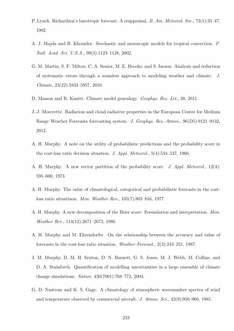
P. Lynch. Richardson’s barotropic forecast: A reappraisal. B. Am. Meteorol. Soc., 73(1):35–47,
1992.
A. J. Majda and B. Khouider. Stochastic and mesoscopic models for tropical convection. P.
Natl. Acad. Sci. U.S.A., 99(3):1123–1128, 2002.
G. M. Martin, S. F. Milton, C. A. Senior, M. E. Brooks, and S. Ineson. Analysis and reduction
of systematic errors through a seamless approach to modeling weather and climate. J.
Climate, 23(22):5933–5957, 2010.
D. Masson and R. Knutti. Climate model genealogy. Geophys. Res. Let., 38, 2011.
J.-J. Morcrette. Radiation and cloud radiative properties in the European Centre for Medium
Range Weather Forecasts forecasting system. J. Geophys. Res.-Atmos., 96(D5):9121–9132,
2012.
A. H. Murphy. A note on the utility of probabilistic predictions and the probability score in
the cost-loss ratio decision situation. J. Appl. Meteorol., 5(4):534–537, 1966.
A. H. Murphy. A new vector partition of the probability score. J. Appl. Meteorol., 12(4):
595–600, 1973.
A. H. Murphy. The value of climatological, categorical and probabilistic forecasts in the cost-
loss ratio situatiuon. Mon. Weather Rev., 105(7):803–816, 1977.
A. H. Murphy. A new decomposition of the Brier score: Formulation and interpretation. Mon.
Weather Rev., 114(12):2671–2673, 1986.
A. H. Murphy and M. Ehrendorfer. On the relationship between the accuracy and value of
forecasts in the cost-loss ratio situation. Weather Forecast., 2(3):243–251, 1987.
J. M. Murphy, D. M. H. Sexton, D. N. Barnett, G. S. Jones, M. J. Webb, M. Collins, and
D. A. Stainforth. Quantification of modelling uncertainties in a large ensemble of climate
change simulations. Nature, 430(7001):768–772, 2004.
G. D. Nastrom and K. S. Gage. A climatology of atmospheric wavenumber spectra of wind
and temperature observed by commercial aircraft. J. Atmos. Sci., 42(9):950–960, 1985.
233
F. Nebeker. Calculating the Weather: Meteorology in the 20th Century. Academic Press, Inc.,
San Diego, California, U.S.A., 1995.
A. Oort and J. Yienger. Observed interannual variability in the Hadley circulation and its
connection to ENSO. J. Climate, 9(11):2751–2767, 1996.
T. N. Palmer. A nonlinear dynamical perpective on climate change. Weather, 48(10):314–326,
1993.
T. N. Palmer. A nonlinear dynamical perpective on climate prediction. J. Climate, 12(2):
575–591, 1999.
T. N Palmer. A nonlinear dynamical perspective on model error: A proposal for non-local
stochastic-dynamic parametrisation in weather and climate prediction models. Q. J. Roy.
Meteor. Soc., 127(572):279–304, 2001.
T. N Palmer. The economic value of ensemble forecasts as a tool for risk assessment: From
days to decades. Q. J. Roy. Meteor. Soc., 128(581):747–774, 2002.
T. N. Palmer. Towards the probabilistic earth-system simulator: A vision for the future of
climate and weather prediction. Q. J. Roy. Meteor. Soc., 138(665):841–861, 2012.
T. N. Palmer, A. Alessandri, U. Andersen, P. Cantelaube, M. Davey, P. Delecluse, M. Deque,
E. Dıez, F. J. Doblas-Reyes, H. Feddersen, R. Graham, S. Gualdi, J.-F. Gueremy, R. Haged-
orn, M. Hoshen, N. Keenlyside, M. Latif, A. Lazar, E. Maisonnave, V. Marletto, A. P.
Morse, B. Orfila, P Rogel, J.-M. Terres, and M. C. Thomson. Development of a European
multimodel ensemble system for seasonal-to-interannual prediction (DEMETER). B. Am.
Meteorol. Soc., 85(6):853–872, 2004.
T. N. Palmer, F. J. Doblas-Reyes, A. Weisheimer, and M. J. Rodwell. Towards seamless pre-
diction: Calibration of climate change projections using seasonal forecasts. B. Am. Meteorol.
Soc., 89(4):459–470, 2008.
T. N. Palmer, R. Buizza, F. Doblas-Reyes, T. Jung, M. Leutbecher, G. J. Shutts, M. Stein-
heimer, and A. Weisheimer. Stochastic parametrization and model uncertainty. Technical
Report 598, European Centre for Medium-Range Weather Forecasts, Shinfield park, Read-
ing, 2009.
234

C. Pennell and T. Reichler. On the effective number of climate models. J. Climate, 24(9):
2358–2367, 2011.
K. Peters, C. Jakob, L. Davies, B. Khouider, and A. J. Majda. Stochastic behavior of tropical
convection in observations and a multicloud model. J. Atmos. Sci., 2013. In press.
R. S. Plant and G. C. Craig. A stochastic parameterization for deep convection based on
equilibrium statistics. J. Atmos. Sci., 65(1):87–104, 2008.
B. Pohl and N. Fauchereau. The southern annular mode seen through weather regimes. J.
Climate, 25(9):3336–3354, 2012.
D. Pollard. A User’s Guide to Measure Theoretic Probability. Cambridge University Press,
Cambridge, U.K. and New York, NY, U.S.A., 2002.
L. Ricciardulli and R. R. Garcia. The excitation of equatorial waves by deep convection in the
NCAR community climate model (CCM3). J. Atmos. Sci., 57(21):3461–3487, 2000.
D. S. Richardson. Measures of skill and value of ensemble prediction systems, their interre-
lationship and the effect of ensemble size. Q. J. Roy. Meteor. Soc., 127(577):2473–2489,
2001.
L. F. Richardson. Weather Prediction by Numerical Process. Cambridge University Press, The
Edinburgh Building, Cambridge, CB2 8RU, England, 2nd edition, 2007.
M. J. Rodwell and T. N. Palmer. Using numerical weather prediction to assess climate models.
Q. J. Roy. Meteor. Soc., 133(622):129–146, 2007.
J. Rougier, D. M. H. Sexton, J. M. Murphy, and D. Stainforth. Analyzing the climate sensitivity
of the HadSM3 climate model using ensembles from different but related experiments. J.
Climate, 22:3540–3557, 2009.
M. S. Roulston and L. A. Smith. Evaluating probabilistic forecasts using information theory.
Mon. Weather Rev., 130(6):1653–1660, 2002.
M. S. Roulston and L. A. Smith. The boy who cried wolf revisited: The impact of false alarm
intolerance on cost-loss scenarios. Weather Forecast., 19(2):391–397, 2004.
F. Sanders. On subjective probability forecasting. J. Appl. Meteorol., 2(2):191–201, 1963.
235

B. M. Sanderson. A multimodel study of parametric uncertainty in predictions of climate
response to rising greenhouse gas concentrations. J. Climate, 24(5):1362–1377, 2011.
B. M. Sanderson, C. Piani, W. J. Ingram, D. A. Stone, and M. R. Allen. Towards constraining
climate sensitivity by linear analysis of feedback patterns in thousands of perturbed-physics
GCM simulations. Clim. Dynam., 30(2–3):175–190, 2008.
G. Shutts. A kinetic energy backscatter algorithm for use in ensemble prediction systems. Q.
J. Roy. Meteor. Soc., 131(612):3079–3102, 2005.
G. J. Shutts. Stochastic backscatter in the unified model. Met Office Scientific Advisory
Committee Paper 14.5, U.K. Met Office, FitzRoy Road, Exeter, 2009.
G. J. Shutts and M. E. B. Gray. A numerical modelling study of the geostrophic adjustment
process following deep convection. Q. J. Roy. Meteor. Soc., 120(519):1145–1178, 1994.
G. J. Shutts and T. N. Palmer. Convective forcing fluctuations in a cloud-resolving model:
Relevance to the stochastic parameterization problem. J. Climate, 20(2):187–202, 2007.
J. Slingo and T. N. Palmer. Uncertainty in weather and climate prediction. Phil. Trans. R.
Soc. A, 369(1956), 2011.
S. Solomon, D. Qin, M. Manning, Z. Chen, M. Marquis, K. B. Averyt, Tignor M., and H. L.
Miller. Summary for policymakers. In Climate Change 2007: The Physical Science Basis.
Contribution of Working Group I to the Fourth Assessment Report of the Intergovernmental
Panel on Climate Change, Cambridge, United Kingdom and New York, NY, USA, 2007.
Cambridge University Press.
D. A Stainforth, T. Aina, C. Christensen, M. Collins, N. Faull, D. J. Frame, J. A. Kettlebor-
ough, S. Knight, A. Martin, J. M. Murphy, C. Piani, D. Sexton, L. A. Smith, R. A Spicer,
A. J. Thorpe, and M. R Allen. Uncertainty in predictions of the climate response to rising
levels of greenhouse gases. Nature, 433(7024):403–406, 2005.
D. J. Stensrud. Upscale effects of deep convection during the North American monsoon. J.
Atmos. Sci., 70(9):2681–2695, 2013.
236
D. J. Stensrud, J.-W. Bao, and T. T. Warner. Using initial condition and model physics
perturbations in short-range ensemble simulations of mesoscale convective systems. Mon.
Weather Rev., 128(7):2077–2107, 2000.
E. M. Stephens, T. L. Edwards, and D. Demeritt. Communicating probabilistic information
from climate model ensembles — lessons from numerical weather prediction. WIREs: Clim.
Change, 3(5):409–426, 2012.
D. B. Stephenson, A. Hannachi, and A. O’Neill. On the existence of multiple climate regimes.
Q. J. Roy. Meteor. Soc., 130(597):583–605, 2004.
D. M. Straus, S. Corti, and F. Molteni. Circulation regimes: Chaotic variability versus sst-
forced predictability. J. Climate, 20(10):2251–2272, 2007.
K. E. Taylor, R. J. Stouffer, and G. A. Meehl. An overview of CMIP5 and the experiment
design. B. Am. Meteorol. Soc., 93(4):485–498, 2012.
M. Tiedtke. A comprehensive mass flux scheme for cumulus parameterization in large-scale
models. Mon. Weather Rev., 117(8):1779–1800, 1989.
M. Tiedtke. Representation of clouds in large-scale models. Mon. Weather Rev., 121(11):
3040–3061, 1993.
J. Todter and B. Ahrens. Generalisation of the ignorance score: Continuous ranked version
and its decomposition. Mon. Weather Rev., 140(6):2005–2017, 2012.
N. P. Wedi. The numerical coupling of the physical parametrizations to the “dynamical”
equations in a forecast model. Technical Report 274, European Centre for Medium-Range
Weather Forecasts, Shinfield park, Reading, 1999.
A. P. Weigel, M. A. Liniger, and C. Appenzeller. Can multi-model combination really enhance
the prediction skill of probabilistic ensemble forecasts? Q. J. Roy. Meteor. Soc., 134(630):
241–260, 2008.
A. Weisheimer, T. N. Palmer, and F. J. Doblas-Reyes. Assessment of representations of model
uncertainty. Geophys. Res. Let., 38, 2011.
237

D. S. Wilks. Effects of stochastic parametrizations in the Lorenz ’96 system. Q. J. Roy. Meteor.
Soc., 131(606):389–407, 2005.
D. S. Wilks. Statistical Methods in the Atmospheric Sciences, volume 91 of International
Geophysics Series. Elsevier, second edition, 2006.
K.-M. Xu, A. Arakawa, and S. K. Krueger. The macroscopic behavior of cumulus ensembles
simulated by a cumulus ensemble model. J. Atmos. Sci., 49(24):2402–2420, 1992.
T. Yokohata, M. J. Webb, M. Collins, K. D. Williams, M. Yoshimori, J. C. Hargreaves, and
J. D. Annan. Structural similarities and differences in climate responses to CO2 increase
between two perturbed physics ensembles. J. Climate, 23(6):1392–1410, 2010.
Y. Zhu, Z. Toth, R. Wobus, D. Richardson, and K. Mylne. The economic value of ensemble-
based weather forecasts. B. Am. Meteorol. Soc., 83(1):73–83, 2002.
238