Stochastic optimization, multivariate numerical integration andQuasi-Monte Carlo methods

W. Romisch

Humboldt-University BerlinInstitute of Mathematics

www.math.hu-berlin.de/~romisch

Chemnitzer Mathematisches Colloquium, TU Chemnitz, 29.6.2017

Introduction and overview

• Stochastic optimization: Mathematics of decision making under uncertainty.

• Two-stage stochastic optimization is a standard problem. But, the evaluation

of the objective of such models is #P-hard (Hanasusanto-Kuhn-Wiesemann 16).

• Computational methods for solving stochastic optimization problems require

a discretization of the underlying probability distribution induced by a nu-

merical integration scheme for computing expectations.

• Standard approach: Variants of Monte Carlo (MC) methods. However, MC

methods are extremely slow and may require enormous sample sizes.

• On the other hand, it is known that numerical integration is strongly polyno-

mially tractable for integrands belonging to weighted tensor product mixed

Sobolev spaces if the weights satisfy certain condition (Sloan-Wozniakowski 98).

• Moreover, the optimal order of convergence of numerical integration in such

spaces can essentially be achieved by certain randomized Quasi-Monte Carlo

methods (Sloan-Kuo-Joe 02, Kuo 03).

• Typical integrands in two-stage stochastic programming can be approximated

by functions from mixed Sobolev spaces if their effective dimension is low.

Application: Mean-Risk Electricity Portfolio Management

(Eichhorn-Romisch-Wegner 05, Eichhorn-Heitsch-Romisch 10)

Linear two-stage stochastic programming models

Consider a linear program with stochastic parameters of the form

min〈c, x〉 : x ∈ X, T (ξ)x = h(ξ),where ξ : Ω → Ξ is a random vector defined on a probability space (Ω,F ,P),

c ∈ Rm, Ξ and X are polyhedral subsets of Rd and Rm, respectively, and the

r ×m-matrix T (·) and vector h(·) ∈ Rr are affine functions of ξ.

Idea: Introduce a recourse variable y ∈ Rm, recourse costs q(·) ∈ Rm as affine

function of ξ, a fixed recourse r×m-matrix W , a polyhedral cone Y ⊆ Rm, and

solve the second-stage or recourse program

min〈q(ξ), y〉 : y ∈ Y,Wy = h(ξ)− T (ξ)x.Define the optimal recourse costs

Q(x, ξ) := Φ(q(ξ), h(ξ)− T (ξ)x) = inf〈q(ξ), y〉 : y ∈ Y,Wy = h(ξ)− T (ξ)xand add the expected recourse costs E[Q(x, ξ)] (depending on the first-stage

decision x) to the original objective and consider the two-stage program

min〈c, x〉 + E[Q(x, ξ)] : x ∈ X

.

Structural properties of two-stage models

We consider the infimum function Φ(·, ·) of the parametrized linear (second-

stage) program, namely,

Φ(u, t) = inf〈u, y〉 : Wy = t, y ∈ Y

((u, t) ∈ Rm × Rr)

= sup〈t, z〉 : W>z − u ∈ Y ∗

((u, t) ∈ D ×W (Y ))

D =u ∈ Rm : z ∈ Rr : W>z − u ∈ Y ∗

6= ∅

where W> denotes the transposed of the recourse matrix W and Y ? the polar

cone of Y and we used linear programming duality.

Theorem: (Walkup-Wets 69)

The function Φ(·, ·) is finite and continuous on the polyhedral cone D×W (Y ).

Furthermore, the function Φ(u, ·) is piecewise linear convex on W (Y ) for fixed

u ∈ D, and Φ(·, t) is piecewise linear concave on D for fixed t ∈ W (Y ).

There exists a decompostion of D × W (Y ) into polyhedral cones Kj, j =

1, . . . , `, and m× r matrices Cj such that

Φ(u, t) = maxj=1,...,`

〈Cju, t〉.

Assumptions:

(A1) relatively complete recourse: for any (ξ, x) ∈ Ξ×X ,

h(ξ)− T (ξ)x ∈ W (Y );

(A2) dual feasibility: q(ξ) ∈ D holds for all ξ ∈ Ξ.

(A3) finite second order moment:∫

Ξ ‖ξ‖2P (dξ) <∞.

Note that (A1) is satisfied if W (Y ) = Rd (complete recourse). In general, (A1)

and (A2) impose a condition on the support of P .

Proposition: (Wets 74)

Assume (A1) and (A2). Then the deterministic equivalent of the two-stage

model represents a convex program (with linear constraints) if the integrals∫Ξ Φ(q(ξ), h(ξ)−T (ξ)x)P (dξ) are finite for all x ∈ X . For the latter it suffices

to assume (A3).

An element x ∈ X minimizes the convex two-stage program if and only if

0 ∈∫

Ξ

∂Q(x, ξ)P (dξ) + NX(x) ,

∂Q(x, ξ) = c− T (ξ)> arg maxz∈Rr,W>z−q(ξ)∈Y ?

〈z, h(ξ)− T (ξ)x〉.

Complexity of two-stage stochastic programs

The two papers Dyer-Stougie 06, Hanasusanto-Kuhn-Wiesemann 16 consider the following

second-stage optimal value function

Q(α, β, ξ)= maxξ>y − βz : y ≤ αz, y ∈ Rd

+, z ∈ [0, 1]

= maxξ>α− β, 0,

where α ∈ Rd+ and β ∈ R+ are parameters and the random vector ξ is uniformly

distributed in [0, 1]d. Starting with the identity

maxγ − β, 0 = γ −∫ β

0

1lγ≥tdt

we find for the expected recourse function

E[Q(α, β, ξ)] = E[α>ξ]−∫ β

0

E[

1lα>ξ≥t

]dt

=1

2α>e− β +

∫ β

0

VolP (α, t)dt

∂E[Q(α, β, ξ)]

∂β= VolP (α, β)− 1 ,

where P (α, β) = z ∈ [0, 1]d : α>z ≤ β is the knapsack polytope and

e = (1, . . . , 1)> ∈ Rd.

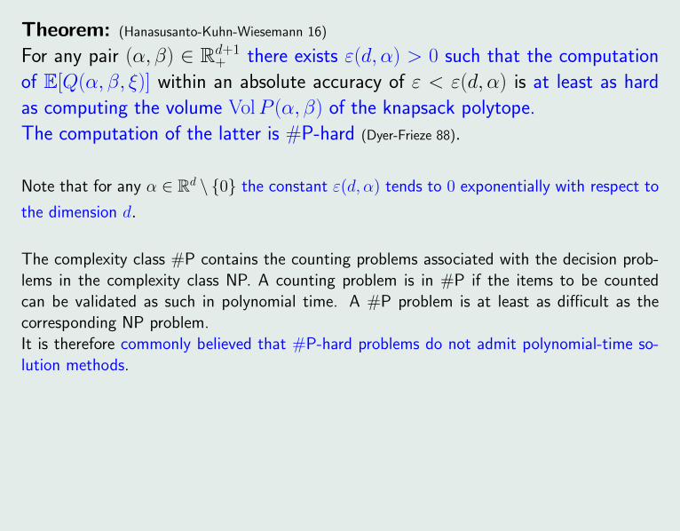
Theorem: (Hanasusanto-Kuhn-Wiesemann 16)

For any pair (α, β) ∈ Rd+1+ there exists ε(d, α) > 0 such that the computation

of E[Q(α, β, ξ)] within an absolute accuracy of ε < ε(d, α) is at least as hard

as computing the volume VolP (α, β) of the knapsack polytope.

The computation of the latter is #P-hard (Dyer-Frieze 88).

Note that for any α ∈ Rd \ 0 the constant ε(d, α) tends to 0 exponentially with respect to

the dimension d.

The complexity class #P contains the counting problems associated with the decision prob-lems in the complexity class NP. A counting problem is in #P if the items to be countedcan be validated as such in polynomial time. A #P problem is at least as difficult as thecorresponding NP problem.It is therefore commonly believed that #P-hard problems do not admit polynomial-time so-lution methods.

Note also that the function

f (ξ) = maxξ>α− β, 0 (ξ ∈ [0, 1]d)

is not of bounded variation in the sense of Hardy and Krause if d > 2 (Owen 05)

and does not have mixed Sobolev derivatives on [0, 1]d.

But, both properties are particularly relevant for the application of Quasi-Monte

Carlo methods for numerical integration.

For general linear two-stage stochastic programs, the second-stage optimal value

function Φ(q(·), h(·)− T (·)x) is continuous and piecewise linear-quadratic on Ξ

if (A1) and (A2) is satisfied. It holds

Φ(q(ξ), h(ξ)− T (ξ)x) = maxj=1,...,`

(Cjq(ξ))>(h(ξ)− T (ξ)x) ((x, ξ) ∈ X × Ξ),

for some ` ∈ N and r ×m-matrices Cj, j = 1, . . . , `. The latter correspond to

some decomposition of D ×W (Y ) into ` polyhedral cones.

Discrete approximations of two-stage models

Replace the (original) probability measure P by measures Pn having (finite) dis-

crete support ξ1, . . . , ξn (n ∈ N), i.e.,

Pn =

n∑i=1

wiδξi,

and insert it into the infinite-dimensional stochastic program:

min〈c, x〉 +

n∑i=1

wi〈q(ξi), yi〉 : x ∈ X, yi ∈ Y, i = 1, . . . , n,

Wy1 +T (ξ1)x = h(ξ1)

Wy2 +T (ξ2)x = h(ξ2). . . ... = ...

Wyn +T (ξn)x = h(ξn)Hence, we arrive at an (often) large scale block-structured linear program which

is solvable in polynomial time and allows for specific decomposition methods.

(Ruszczynski-Shapiro 2003, Kall-Mayer 2005 (2010))

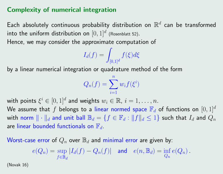
Complexity of numerical integration

Each absolutely continuous probability distribution on Rd can be transformed

into the uniform distribution on [0, 1]d (Rosenblatt 52).

Hence, we may consider the approximate computation of

Id(f ) =

∫[0,1]d

f (ξ)dξ

by a linear numerical integration or quadrature method of the form

Qn(f ) =

n∑i=1

wif (ξi)

with points ξi ∈ [0, 1]d and weights wi ∈ R, i = 1, . . . , n.

We assume that f belongs to a linear normed space Fd of functions on [0, 1]d

with norm ‖ · ‖d and unit ball Bd = f ∈ Fd : ‖f‖d ≤ 1 such that Id and Qn

are linear bounded functionals on Fd.

Worst-case error of Qn over Bd and minimal error are given by:

e(Qn) = supf∈Bd|Id(f )−Qn(f )| and e(n,Bd) = inf

Qne(Qn) .

(Novak 16)

It is known that due to the convexity and symmetry of Bd linear algorithms are

optimal among nonlinear and adaptive ones (Bakhvalov 71, Novak 88).

The information complexity n(ε,Bd) is the minimal number of function values

which is needed that the worst-case error is at most ε, i.e.,

n(ε,Bd) = minn : ∃Qn such that e(Qn) ≤ ε

Of course, the behavior of n(ε,Bd) as function of (ε, d) depends heavily on Fd.

Numerical integration is said to

be polynomially tractable if there exist constants C > 0 q ≥ 0, p > 0 such that

n(ε,Bd) ≤ Cdqε−p ,

be strongly polynomially tractable if there exist constants C > 0, p > 0 such

that

n(ε,Bd) ≤ Cε−p ,

have the curse of dimension if there exist c > 0, ε0 > 0 and γ > 0 such that

n(ε,Bd) ≥ c(1 + γ)d for all ε ≤ ε0 and for infinitely many d ∈ N.

Randomized algorithms:

A randomized quadrature algorithm is denoted by (Q(ω))ω∈Ω and considered on

a probability space (Ω,F ,P).. We assume that Q(ω) is a quadrature algorithm

for each ω and that it depends on ω in a measurable way. Let n(f, ω) denote

the number of evaluations of f ∈ Fd needed to perform Q(ω)f . The number

n(Q) = supf∈Bd

∫Ω

n(f, ω)P(dω)

is called the cardinality of the randomized algorithm Q and

eran(Q) = supf∈Bd

(∫Ω

|Idf −Q(ω)f |2 P(dω))1

2

the error of Q. The minimal error of randomized algorithms is

eran(n,Bd) = inferan(Q) : n(Q) ≤ n .By construction it is clear that eran(n,Bd) ≤ e(n,Bd) holds.

Standard Monte Carlo (MC) method Q based on n i.i.d. samples: (Mathe 95)

eran(Q) = (1 +√n)−1 ≤ n−

12

if Bd is the unit ball of Fd = Lp([0, 1]d) for 2 ≤ p <∞.

Example:Consider the Banach space Fd = Cr([0, 1]d) (r ∈ N) with the norm

‖f‖r,d = max|α|≤r‖Dαf‖∞,

where α = (α1, . . . , αd) ∈ Nd0 and Dαf denotes the mixed partial derivative of

order |α| =∑d

i=1 αi, i.e.,

Dαf (ξ) =∂|α|f

∂ξα11 · · · ∂ξαdd

(ξ) .

It is long known (Bakhvalov 59) that there exist constants Cr,d, cr,d > 0 such that

cr,d n− rd ≤ e(n,Bd) ≤ Cr,d n

− rd .

But, surprisingly it was shown only recently that the numerical integration on

Cr([0, 1]d) suffers from the curse of dimension (Hinrichs-Novak-Ullrich-Wozniakowski 14).

For the tensor product mixed Sobolev space

W(r,...,r)2,mix ([0, 1]d) = f : [0, 1]d → R : Dαf ∈ L2([0, 1]d) if ‖α‖∞ ≤ r

it is known that e(n,Bd) = O(n−r(log n)(d−1)

2 ) (Frolov 76, Bykovskii 85).

We consider the linear space W 12,γ([0, 1]) of all absolutely continuous functions

on [0, 1] with derivatives belonging to L2([0, 1]) and the weighted inner product

〈f, g〉γ =

∫ 1

0

f (x)dx

∫ 1

0

g(x)dx +1

γ

∫ 1

0

f ′(x)g′(x)dx.

Then the weighted tensor product mixed Sobolev space

W(1,...,1)2,γ,mix([0, 1]d) =

d⊗j=1

W 12,γj

([0, 1])

is equipped with the inner product

〈g, g〉γ =∑u⊆D

γ−1u

∫[0,1]|u|

(∫[0,1]d−|u|

∂|u|

∂tug(t)dt−u

)(∫[0,1]d−|u|

∂|u|

∂tug(t)dt−u

)dtu ,

where D = 1, . . . , d, the weights γi are positive and γu is given in product form γu =∏

i∈u γi

for u ⊆ D, where γ∅ = 1. For u ⊆ D we use the notation |u| for its cardinality, −u for D \ uand tu for the |u|-dimensional vector with components tj for j ∈ u.

Theorem: (Sloan-Wozniakowski 98, Sloan-Wang-Wozniakowski 04)

Numerical integration is strongly polynomially tractable on W(1,...,1)2,γ,mix([0, 1]d) if

∞∑j=1

γj <∞ .

Monte Carlo sampling

Monte Carlo methods are based on drawing independent identically distributed

(i.i.d.) Ξ-valued random samples ξ1(·), . . . , ξn(·), . . . (defined on some probabil-

ity space (Ω,A,P)) from an underlying probability distribution P (on Ξ) such

that

Qn(ω)(f ) =1

n

n∑i=1

f (ξi(ω)),

i.e., Qn(·) is a random functional, and it holds

limn→∞

Qn(ω)(f ) =

∫Ξ

f (ξ)P (dξ) = E(f ) P-almost surely

for every real continuous and bounded function f on Ξ.

If P has a finite moment of order r ≥ 1, the error estimate

E

[∣∣∣∣∣1nn∑i=1

f (ξi(ω))− E(f )

∣∣∣∣∣r]≤ E [(f − E(f ))r]

nr−1

is valid.

(Shapiro-Dentcheva-Ruszczynski 2009 (2014))

Hence, the mean square convergence rate is

‖Qn(ω)(f )− E(f )‖L2 = σ(f )n−12 ,

where σ2(f ) = E[(f − E(f ))2

]is assumed to be finite.

Advantages:

(i) MC sampling works for (almost) all integrands.

(ii) The machinery of probability theory is available.

(iii) The convergence rate does not depend on d.

Deficiencies: (Niederreiter 92)

(i) There exist ’only’ probabilistic error bounds.

(ii) Possible regularity of the integrand does not improve the rate.

(iii) Generating (independent) random samples is difficult.

Practically, iid samples are approximately obtained by pseudo random number

generators as uniform samples in [0, 1]d and later transformed to more general

sets Ξ and distributions P .

Good pseudo random number generator: Mersenne Twister (Matsumoto-Nishimura 98)

Quasi-Monte Carlo methods

The basic idea of Quasi-Monte Carlo (QMC) methods is to use deterministic

points that are (in some way) uniformly distributed in [0, 1]d and to consider the

approximate computation of

Id(f ) =

∫[0,1]d

f (ξ)dξ

by a QMC algorithm with (non-random) points ξi, i = 1, . . . , n, from [0, 1]d:

Qn(f ) =1

n

n∑i=1

f (ξi)

The uniform distribution property of point sets may be defined in terms of the

so-called Lp-discrepancy of ξ1, . . . , ξn for 1 ≤ p ≤ ∞

dp,n(ξ1, . . . , ξn) =(∫

[0,1]d|disc(ξ)|pdξ

)1p, disc(ξ) :=

d∏j=1

ξj −1

n

n∑i=1

1l[0,ξ)(ξi) .

There exist sequences (ξi) in [0, 1]d such that for all δ ∈ (0, 12]

d∞,n(ξ1, . . . , ξn) = O(n−1(log n)d) or d∞,n(ξ1, . . . , ξn) ≤ C(d, δ)n−1+δ .

Randomly shifted lattice rules

We consider the randomized Quasi-Monte Carlo method

Qn(ω)(f ) =1

n

n∑i=1

f((i− 1)

ng +4(ω)

),

where 4 is a random vector with uniform distribution on [0, 1]d.

Theorem:Let n be prime, Bd be the unit ball in W (1,...,1)

2,γ,mix([0, 1]d). Then g ∈ Zd can be

constructed component-by-component such that for any δ ∈ (0, 12] there exists a

constant C(δ) > 0 and the randomized minimal error allows the estimate

eran(Qn,Bd) ≤ C(δ)n−1+δ ,

where the constant C(δ) increases when δ decreases, but does not depend on

the dimension d if the sequence (γj) satisfies the condition

∞∑j=1

γ1

2(1−δ)j <∞ (e.g. γj = 1

j3).

(Sloan-Kuo-Joe 02, Kuo 03, Nuyens-Cools 06)

ANOVA decomposition and effective dimension

We consider a multivariate function f : Rd → R and intend to compute the

mean of f (ξ), i.e.

E[f (ξ)] = Id,ρ(f ) =

∫Rdf (ξ1, . . . , ξd)ρ(ξ1, . . . , ξd)dξ1 · · · dξd ,

where ξ is a d-dimensional random vector with density

ρ(ξ) =

d∏k=1

ρk(ξk) (ξ ∈ Rd).

We are interested in a representation of f consisting of 2d terms

f (ξ) = f0 +

d∑i=1

fi(ξi) +

d∑i,j=1i<j

fij(ξi, ξj) + · · · + f12···d(ξ1, . . . , ξd).

The previous representation can be more compactly written as

(∗) f (ξ) =∑u⊆D

fu(ξu) ,

where D = 1, . . . , d and ξu contains only the components ξj with j ∈ u and

belongs to R|u|. Here, |u| denotes the cardinality of u.

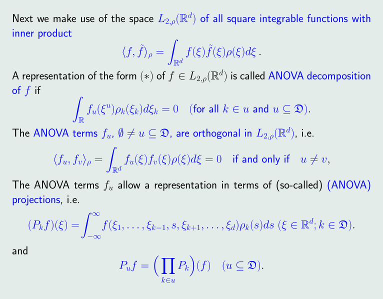
Next we make use of the space L2,ρ(Rd) of all square integrable functions with

inner product

〈f, f〉ρ =

∫Rdf (ξ)f (ξ)ρ(ξ)dξ .

A representation of the form (∗) of f ∈ L2,ρ(Rd) is called ANOVA decomposition

of f if ∫Rfu(ξ

u)ρk(ξk)dξk = 0 (for all k ∈ u and u ⊆ D).

The ANOVA terms fu, ∅ 6= u ⊆ D, are orthogonal in L2,ρ(Rd), i.e.

〈fu, fv〉ρ =

∫Rdfu(ξ)fv(ξ)ρ(ξ)dξ = 0 if and only if u 6= v,

The ANOVA terms fu allow a representation in terms of (so-called) (ANOVA)

projections, i.e.

(Pkf )(ξ) =

∫ ∞−∞f (ξ1, . . . , ξk−1, s, ξk+1, . . . , ξd)ρk(s)ds (ξ ∈ Rd; k ∈ D).

and

Puf =(∏k∈u

Pk

)(f ) (u ⊆ D).

Then it holds (Kuo-Sloan-Wasilkowski-Wozniakowski 10):

fu =(∏j∈u

(I − Pj))P−u(f ) = P−u(f ) +

∑v(u

(−1)|u|−|v|P−v(f ) ,

Consider the variances of f and fu

σ2(f ) = ‖f − Id,ρ(f )‖22,ρ und σ2

u(f ) = ‖fu‖22,ρ

and obtain

σ2(f ) = ‖f‖2L2− (Id,ρ(f ))2 =

∑∅6=u⊆D

σ2u(f ) .

For small ε ∈ (0, 1) (e.g. ε = 0.01)

dS(ε) = mins ∈ D :

∑|u|≤s

σ2u(f )

σ2(f )≥ 1− ε

is called effective (superposition) dimension of f and it holds

(+)∥∥∥f − ∑

|u|≤dS(ε)

fu

∥∥∥2,ρ≤√εσ(f ) ,

i.e., the function f is approximated by a truncated ANOVA decomposition which contains

all ANOVA terms fu such that |u| ≤ dS(ε). If f is nonsmooth and the ANOVA terms fu,

|u| ≤ dS(ε), are smoother than f , the estimate (+) means an approximate smoothing of f .

ANOVA decomposition of two-stage integrands

Assumptions: (A1) and (A2)(A3) P has fourth order absolute moments.

(A4) P has a density of the form ρ(ξ) =∏d

i=1 ρi(ξi) (ξ ∈ Rd) with continuous

marginal densities ρi, i ∈ D.

(A5) For each x ∈ X all common faces of adjacent convex polyhedral sets

Ξj(x) = ξ ∈ Ξ : (q(ξ), h(ξ)− T (ξ)x) ∈ Kj (j = 1, . . . , `)

do not parallel any coordinate axis, where the polyhedral cones Kj,j = 1, . . . , `, decompose dom Φ = D ×W (Y ) (geometric condition).

Theorem: Let x ∈ X , assume (A1)–(A5) and f = f (x, ·) be the two-stage

integrand. Then the second order truncated ANOVA decomposition of f

f (2) :=∑|u|≤2

fu where f = f (2) +

d∑|u|=3

fu

belongs to W(1,...,1)2,ρ,mix (Rd) if all marginal densities ρk, k ∈ D, belong to C1(R).

Remark: The second order truncated ANOVA decomposition f (2) is a good

approximation of f if the effective superposition dimension dS(ε) is at most 2.

Conclusions

• The approximate computation of the objective of linear two-stage stochastic

programs with fixed recourse with a sufficiently high accuracy is #P-hard.

• The numerical integration on weighted tensor product mixed Sobolev spaces

on [0, 1]d is strongly polynomially tractable if the weights satisfy a suitable

condition.

• Randomly shifted lattice rules attain the optimal order of convergence on

such spaces if the weights satisfy a slightly stronger condition. Hence, such

methods are superior to Monte Carlo methods and reduce the sample sizes

from n to almost√n.

• The second order ANOVA decomposition of two-stage integrands belongs to

a mixed Sobolev space on Rd if the marginal densities are in C1 and represent

a good L2,ρ(Rd) approximation if the effective superposition dimension dS(ε)

of the integrands is at most two. It is conjectured that this result extends to

higher effective dimensions.

References:

M. Dyer and L. Stougie: Computational complexity of stochastic programming problems, Mathematical Pro-gramming 106 (2006), 423–432.

J. Dick, F. Y. Kuo and I. H. Sloan: High-dimensional integration – the Quasi-Monte Carlo way, Acta Numerica22 (2013), 133–288.

G. A. Hanasusanto, D. Kuhn and W. Wiesemann: A comment on ”computational complexity of stochasticprogramming problems”, Mathematical Programming 159 (2016), 557–569.

A. Hinrichs, E. Novak, M. Ullrich and H. Wozniakowski: The curse of dimensionality for numerical integrationof smooth functions, Mathematics of Computation 83 (2014), 2853–2863.

F. Y. Kuo: Component-by-component constructions achieve the optimal rate of convergence in weighted Ko-robov and Sobolev spaces, Journal of Complexity 19 (2003), 301–320.

F. Y. Kuo, I. H. Sloan, G. W. Wasilkowski, H. Wozniakowski: On decomposition of multivariate functions,Mathematics of Computation 79 (2010), 953–966.

H. Leovey and W. Romisch: Quasi-Monte Carlo methods for linear two-stage stochastic programming problems,Mathematical Programming 151 (2015), 315–345.

E. Novak: Some results on the complexity of numerical integration, in Monte Carlo and Quasi-Monte CarloMethods (R. Cools and D. Nuyens eds.), Springer, 2016.

A. B. Owen: The dimension distribution and quadrature test functions, Statistica Sinica 13 (2003), 1–17.

A. Ruszczynski and A. Shapiro (Eds.): Stochastic Programming, Handbooks in Operations Research and Man-agement Science, Volume 10, Elsevier, Amsterdam 2003.

I. H. Sloan and H. Wozniakowski: When are Quasi Monte Carlo algorithms efficient for high-dimensional inte-gration, Journal of Complexity 14 (1998), 1–33.

I. H. Sloan, F. Y. Kuo and S. Joe: Constructing randomly shifted lattice rules in weighted Sobolev spaces, SIAMJournal Numerical Analysis 40 (2002), 1650–1665.