stochastic calculus for finance - michigan state...
TRANSCRIPT
Stochastic Calculus for Finance
Albert Cohen
Actuarial Sciences ProgramDepartment of Mathematics
Department of Statistics and ProbabilityA336 Wells Hall
Michigan State UniversityEast Lansing MI
[email protected]@stt.msu.edu
Albert Cohen (MSU) STT 888: Stochastic Calculus for Finance MSU 2016 1 / 249

Course Information
Syllabus to be posted on class page in first week of classes
Homework assignments will posted there as well
Page can be found athttps://www.stt.msu.edu/Academics/ClassPages/
Albert Cohen (MSU) STT 888: Stochastic Calculus for Finance MSU 2016 2 / 249
Course Information
Many examples within these slides are used with kind permission ofProf. Dmitry Kramkov, Dept. of Mathematics, Carnegie MellonUniversity.
Course Textbook: Stochastic Calculus for Finance (Springer Finance.)
Some examples here will be similar to those practice questionspublicly released by the SOA. Please note the SOA owns thecopyright to these questions.
This book will be our reference, and some questions for assignmentswill be chosen from it. Copyright for all questions used from this bookbelongs to Springer.
From time to time, we will also follow the format of Marcel Finan’s ADiscussion of Financial Economics in Actuarial Models: A Preparationfor the Actuarial Exam MFE/3F. Some proofs from there will bereferenced as well. Please find these notes here
Albert Cohen (MSU) STT 888: Stochastic Calculus for Finance MSU 2016 3 / 249
What are financial securities?
Traded Securities - price given by market.
For example:
StocksCommodities
Non-Traded Securities - price remains to be computed.
Is this always true?
We will focus on pricing non-traded securities.
Albert Cohen (MSU) STT 888: Stochastic Calculus for Finance MSU 2016 4 / 249
How does one fairly price non-traded securities?
By eliminating all unfair prices
Unfair prices arise from Arbitrage Strategies
Start with zero capitalEnd with non-zero wealth
We will search for arbitrage-free strategies to replicate the payoff of anon-traded security
This replication is at the heart of the engineering of financial products
Albert Cohen (MSU) STT 888: Stochastic Calculus for Finance MSU 2016 5 / 249
More Questions
Existence - Does such a fair price always exist?
If not, what is needed of our financial model to guarantee at least onearbitrage-free price?
Uniqueness - are there conditions where exactly one arbitrage-freeprice exists?
Albert Cohen (MSU) STT 888: Stochastic Calculus for Finance MSU 2016 6 / 249
And What About...
Does the replicating strategy and price computed reflect uncertaintyin the market?
Mathematically, if P is a probabilty measure attached to a series ofprice movements in underlying asset, is P used in computing theprice?
Albert Cohen (MSU) STT 888: Stochastic Calculus for Finance MSU 2016 7 / 249

Notation
Forward Contract:
A financial instrument whose initial value is zero, and whose finalvalue is derived from another asset. Namely, the difference of thefinal asset price and forward price:
V (0) = 0,V (T ) = S(T )− F (1)
Value at end of term can be negative - buyer accepts this in exchangefor no premium up front
Albert Cohen (MSU) STT 888: Stochastic Calculus for Finance MSU 2016 8 / 249
Notation
Interest Rate:
The rate r at which money grows. Also used to discount the valuetoday of one unit of currency one unit of time from the present
V (0) =1
1 + r,V (1) = 1 (2)
Albert Cohen (MSU) STT 888: Stochastic Calculus for Finance MSU 2016 9 / 249
Notation
Interest Rate:
The rate r at which money grows. Also used to discount the valuetoday of one unit of currency one unit of time from the present
V (0) =1
1 + r,V (1) = 1 (2)
Albert Cohen (MSU) STT 888: Stochastic Calculus for Finance MSU 2016 9 / 249
An Example of Replication
Forward Exchange Rate: There are two currencies, foreign anddomestic:
SBA = 4 is the spot exchange rate - one unit of B is worth SB
A of Atoday (time 0)
rA = 0.1 is the domestic borrow/lend rate
rB = 0.2 is the foreign borrow/lend rate
Compute the forward exchange rate FBA . This is the value of one unit
of B in terms of A at time 1.
Albert Cohen (MSU) STT 888: Stochastic Calculus for Finance MSU 2016 10 / 249
An Example of Replication: Solution
At time 1, we deliver 1 unit of B in exchange for FBA units of domestic
currency A.
This is a forward contract - we pay nothing up front to achieve this.
Initially borrow some amount foreign currency B, in foreign market togrow to one unit of B at time 1. This is achieved by the initial
amountSBA
1+rB(valued in domestic currency)
Invest the amountFBA
1+rAin domestic market (valued in domestic
currency)
Albert Cohen (MSU) STT 888: Stochastic Calculus for Finance MSU 2016 11 / 249
An Example of Replication: Solution
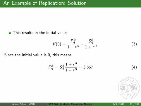
This results in the initial value
V (0) =FBA
1 + rA−
SBA
1 + rB(3)
Since the initial value is 0, this means
FBA = SB
A
1 + rA
1 + rB= 3.667 (4)
Albert Cohen (MSU) STT 888: Stochastic Calculus for Finance MSU 2016 12 / 249
An Example of Replication: Solution
This results in the initial value
V (0) =FBA
1 + rA−
SBA
1 + rB(3)
Since the initial value is 0, this means
FBA = SB
A
1 + rA
1 + rB= 3.667 (4)
Albert Cohen (MSU) STT 888: Stochastic Calculus for Finance MSU 2016 12 / 249
Outline1 Discrete Multiperiod Model
ArbitrageRisk Neutral ProbabilityAmerican OptionsExotic OptionsValuation via Simulation
2 Continuous Model-Ito CalculusBrownian MotionBSMExamplesOptions on FuturesPath Dependent Options
3 Advanced TopicsHeat EquationGeneral Solution of Heat EquationApplication to B-S-M PDE
4 Continuous Model-ProbabilityExpected ValuesApplication of Option GreeksAlbert Cohen (MSU) STT 888: Stochastic Calculus for Finance MSU 2016 13 / 249
Discrete Probability Space
Let us define an event as a point ω in the set of all possible outcomes Ω.This includes the events ”The stock doubled in price over two tradingperiods” or ”the average stock price over ten years was 10 dollars”.
In our initial case, we will consider the simple binary spaceΩ = H,T for a one-period asset evolution. So, given an initialvalue S0, we have the final value S1(ω), with
S1(H) = uS0,S1(T ) = dS0 (5)
with d < 1 < u. Hence, a stock increases or decreases in price,according to the flip of a coin.
Let P be the probability measure associated with these events:
P[H] = p = 1− P[T ] (6)
Albert Cohen (MSU) STT 888: Stochastic Calculus for Finance MSU 2016 14 / 249
Arbitrage
Assume that S0(1 + r) > uS0
Where is the risk involved with investing in the asset S ?
Assume that S0(1 + r) < dS0
Why would anyone hold a bank account (zero-coupon bond)?
Lemma Arbitrage free ⇒ d < 1 + r < u
Albert Cohen (MSU) STT 888: Stochastic Calculus for Finance MSU 2016 15 / 249
Arbitrage
Assume that S0(1 + r) > uS0
Where is the risk involved with investing in the asset S ?
Assume that S0(1 + r) < dS0
Why would anyone hold a bank account (zero-coupon bond)?
Lemma Arbitrage free ⇒ d < 1 + r < u
Albert Cohen (MSU) STT 888: Stochastic Calculus for Finance MSU 2016 15 / 249
Arbitrage
Assume that S0(1 + r) > uS0
Where is the risk involved with investing in the asset S ?
Assume that S0(1 + r) < dS0
Why would anyone hold a bank account (zero-coupon bond)?
Lemma Arbitrage free ⇒ d < 1 + r < u
Albert Cohen (MSU) STT 888: Stochastic Calculus for Finance MSU 2016 15 / 249
Arbitrage
Assume that S0(1 + r) > uS0
Where is the risk involved with investing in the asset S ?
Assume that S0(1 + r) < dS0
Why would anyone hold a bank account (zero-coupon bond)?
Lemma Arbitrage free ⇒ d < 1 + r < u
Albert Cohen (MSU) STT 888: Stochastic Calculus for Finance MSU 2016 15 / 249
Arbitrage
Assume that S0(1 + r) > uS0
Where is the risk involved with investing in the asset S ?
Assume that S0(1 + r) < dS0
Why would anyone hold a bank account (zero-coupon bond)?
Lemma Arbitrage free ⇒ d < 1 + r < u
Albert Cohen (MSU) STT 888: Stochastic Calculus for Finance MSU 2016 15 / 249
Derivative Pricing
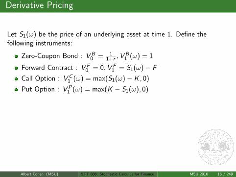
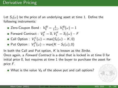
Let S1(ω) be the price of an underlying asset at time 1. Define thefollowing instruments:
Zero-Coupon Bond : V B0 = 1
1+r ,VB1 (ω) = 1
Forward Contract : V F0 = 0,V F
1 = S1(ω)− F
Call Option : V C1 (ω) = max(S1(ω)− K , 0)
Put Option : V P1 (ω) = max(K − S1(ω), 0)
In both the Call and Put option, K is known as the Strike.Once again, a Forward Contract is a deal that is locked in at time 0 forinitial price 0, but requires at time 1 the buyer to purchase the asset forprice F .
What is the value V0 of the above put and call options?
Albert Cohen (MSU) STT 888: Stochastic Calculus for Finance MSU 2016 16 / 249
Derivative Pricing
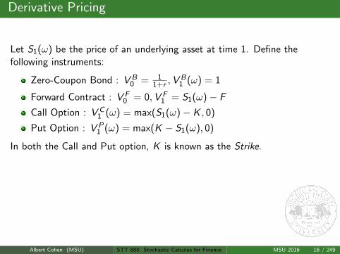
Let S1(ω) be the price of an underlying asset at time 1. Define thefollowing instruments:
Zero-Coupon Bond : V B0 = 1
1+r ,VB1 (ω) = 1
Forward Contract : V F0 = 0,V F
1 = S1(ω)− F
Call Option : V C1 (ω) = max(S1(ω)− K , 0)
Put Option : V P1 (ω) = max(K − S1(ω), 0)
In both the Call and Put option, K is known as the Strike.
Once again, a Forward Contract is a deal that is locked in at time 0 forinitial price 0, but requires at time 1 the buyer to purchase the asset forprice F .
What is the value V0 of the above put and call options?
Albert Cohen (MSU) STT 888: Stochastic Calculus for Finance MSU 2016 16 / 249
Derivative Pricing
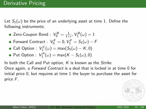
Let S1(ω) be the price of an underlying asset at time 1. Define thefollowing instruments:
Zero-Coupon Bond : V B0 = 1
1+r ,VB1 (ω) = 1
Forward Contract : V F0 = 0,V F
1 = S1(ω)− F
Call Option : V C1 (ω) = max(S1(ω)− K , 0)
Put Option : V P1 (ω) = max(K − S1(ω), 0)
In both the Call and Put option, K is known as the Strike.Once again, a Forward Contract is a deal that is locked in at time 0 forinitial price 0, but requires at time 1 the buyer to purchase the asset forprice F .
What is the value V0 of the above put and call options?
Albert Cohen (MSU) STT 888: Stochastic Calculus for Finance MSU 2016 16 / 249
Derivative Pricing
Let S1(ω) be the price of an underlying asset at time 1. Define thefollowing instruments:
Zero-Coupon Bond : V B0 = 1
1+r ,VB1 (ω) = 1
Forward Contract : V F0 = 0,V F
1 = S1(ω)− F
Call Option : V C1 (ω) = max(S1(ω)− K , 0)
Put Option : V P1 (ω) = max(K − S1(ω), 0)
In both the Call and Put option, K is known as the Strike.Once again, a Forward Contract is a deal that is locked in at time 0 forinitial price 0, but requires at time 1 the buyer to purchase the asset forprice F .
What is the value V0 of the above put and call options?
Albert Cohen (MSU) STT 888: Stochastic Calculus for Finance MSU 2016 16 / 249

Put-Call Parity
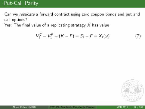
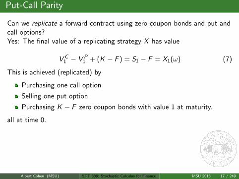
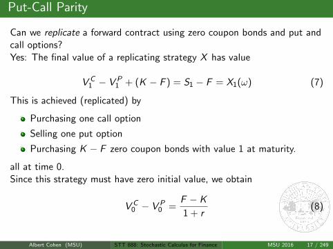
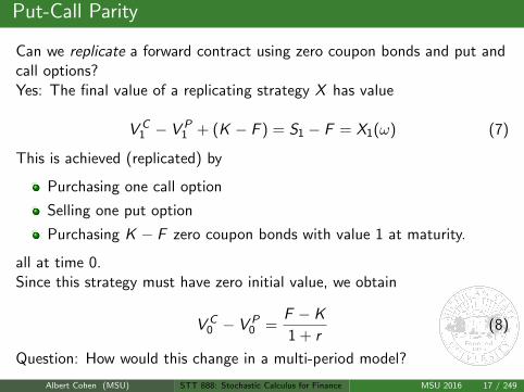
Can we replicate a forward contract using zero coupon bonds and put andcall options?
Yes: The final value of a replicating strategy X has value
V C1 − V P
1 + (K − F ) = S1 − F = X1(ω) (7)
This is achieved (replicated) by
Purchasing one call option
Selling one put option
Purchasing K − F zero coupon bonds with value 1 at maturity.
all at time 0.Since this strategy must have zero initial value, we obtain
V C0 − V P
0 =F − K
1 + r(8)
Question: How would this change in a multi-period model?
Albert Cohen (MSU) STT 888: Stochastic Calculus for Finance MSU 2016 17 / 249
Put-Call Parity
Can we replicate a forward contract using zero coupon bonds and put andcall options?Yes: The final value of a replicating strategy X has value
V C1 − V P
1 + (K − F ) = S1 − F = X1(ω) (7)
This is achieved (replicated) by
Purchasing one call option
Selling one put option
Purchasing K − F zero coupon bonds with value 1 at maturity.
all at time 0.
Since this strategy must have zero initial value, we obtain
V C0 − V P
0 =F − K
1 + r(8)
Question: How would this change in a multi-period model?
Albert Cohen (MSU) STT 888: Stochastic Calculus for Finance MSU 2016 17 / 249
Put-Call Parity
Can we replicate a forward contract using zero coupon bonds and put andcall options?Yes: The final value of a replicating strategy X has value
V C1 − V P
1 + (K − F ) = S1 − F = X1(ω) (7)
This is achieved (replicated) by
Purchasing one call option
Selling one put option
Purchasing K − F zero coupon bonds with value 1 at maturity.
all at time 0.Since this strategy must have zero initial value, we obtain
V C0 − V P
0 =F − K
1 + r(8)
Question: How would this change in a multi-period model?
Albert Cohen (MSU) STT 888: Stochastic Calculus for Finance MSU 2016 17 / 249
Put-Call Parity
Can we replicate a forward contract using zero coupon bonds and put andcall options?Yes: The final value of a replicating strategy X has value
V C1 − V P
1 + (K − F ) = S1 − F = X1(ω) (7)
This is achieved (replicated) by
Purchasing one call option
Selling one put option
Purchasing K − F zero coupon bonds with value 1 at maturity.
all at time 0.Since this strategy must have zero initial value, we obtain
V C0 − V P
0 =F − K
1 + r(8)
Question: How would this change in a multi-period model?
Albert Cohen (MSU) STT 888: Stochastic Calculus for Finance MSU 2016 17 / 249
General Derivative Pricing -One period model
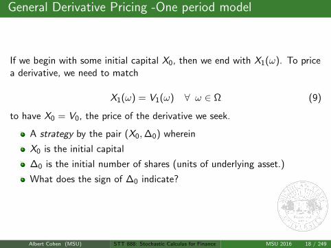
If we begin with some initial capital X0, then we end with X1(ω). To pricea derivative, we need to match
X1(ω) = V1(ω) ∀ ω ∈ Ω (9)
to have X0 = V0, the price of the derivative we seek.
A strategy by the pair (X0,∆0) wherein
X0 is the initial capital
∆0 is the initial number of shares (units of underlying asset.)
What does the sign of ∆0 indicate?
Albert Cohen (MSU) STT 888: Stochastic Calculus for Finance MSU 2016 18 / 249

Replicating Strategy
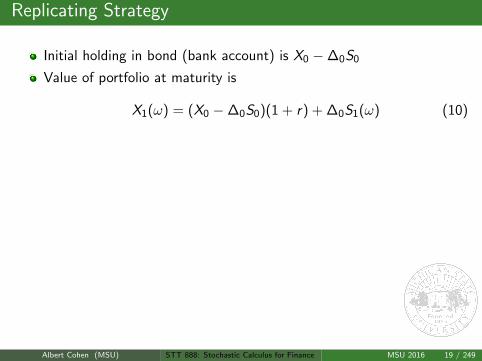
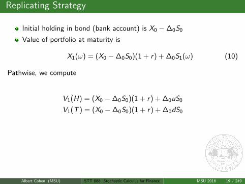
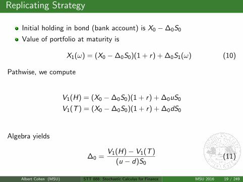
Initial holding in bond (bank account) is X0 −∆0S0
Value of portfolio at maturity is
X1(ω) = (X0 −∆0S0)(1 + r) + ∆0S1(ω) (10)
Pathwise, we compute
V1(H) = (X0 −∆0S0)(1 + r) + ∆0uS0
V1(T ) = (X0 −∆0S0)(1 + r) + ∆0dS0
Algebra yields
∆0 =V1(H)− V1(T )
(u − d)S0(11)
Albert Cohen (MSU) STT 888: Stochastic Calculus for Finance MSU 2016 19 / 249
Replicating Strategy
Initial holding in bond (bank account) is X0 −∆0S0
Value of portfolio at maturity is
X1(ω) = (X0 −∆0S0)(1 + r) + ∆0S1(ω) (10)
Pathwise, we compute
V1(H) = (X0 −∆0S0)(1 + r) + ∆0uS0
V1(T ) = (X0 −∆0S0)(1 + r) + ∆0dS0
Algebra yields
∆0 =V1(H)− V1(T )
(u − d)S0(11)
Albert Cohen (MSU) STT 888: Stochastic Calculus for Finance MSU 2016 19 / 249
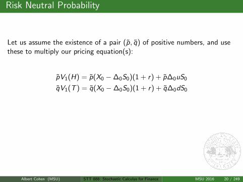
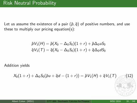
Risk Neutral Probability
Let us assume the existence of a pair (p, q) of positive numbers, and usethese to multiply our pricing equation(s):
pV1(H) = p(X0 −∆0S0)(1 + r) + p∆0uS0
qV1(T ) = q(X0 −∆0S0)(1 + r) + q∆0dS0
Addition yields
X0(1 + r) + ∆0S0(pu + qd − (1 + r)) = pV1(H) + qV1(T ) (12)
Albert Cohen (MSU) STT 888: Stochastic Calculus for Finance MSU 2016 20 / 249
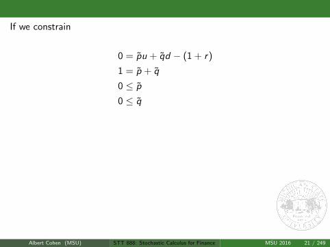
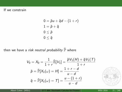
If we constrain
0 = pu + qd − (1 + r)
1 = p + q
0 ≤ p
0 ≤ q
then we have a risk neutral probability P where
V0 = X0 =1
1 + rE[V1] =
pV1(H) + qV1(T )
1 + r
p = P[X1(ω) = H] =1 + r − d
u − d
q = P[X1(ω) = T ] =u − (1 + r)
u − d
Albert Cohen (MSU) STT 888: Stochastic Calculus for Finance MSU 2016 21 / 249
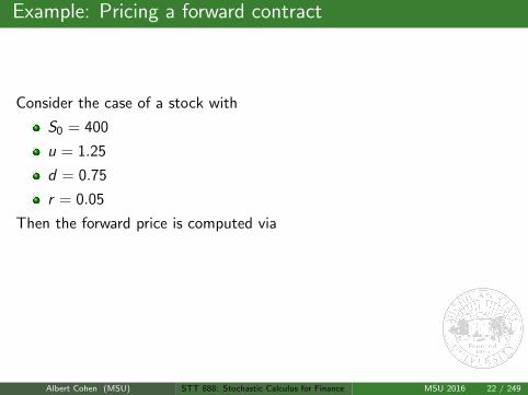
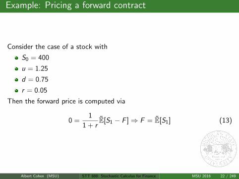
Example: Pricing a forward contract
Consider the case of a stock with
S0 = 400
u = 1.25
d = 0.75
r = 0.05
Then the forward price is computed via
0 =1
1 + rE[S1 − F ]⇒ F = E[S1] (13)
Albert Cohen (MSU) STT 888: Stochastic Calculus for Finance MSU 2016 22 / 249
Example: Pricing a forward contract
Consider the case of a stock with
S0 = 400
u = 1.25
d = 0.75
r = 0.05
Then the forward price is computed via
0 =1
1 + rE[S1 − F ]⇒ F = E[S1] (13)
Albert Cohen (MSU) STT 888: Stochastic Calculus for Finance MSU 2016 22 / 249
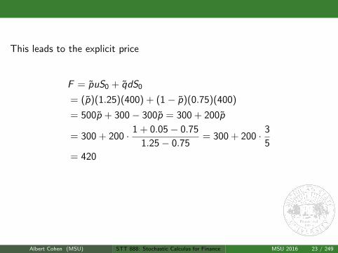
This leads to the explicit price
F = puS0 + qdS0
= (p)(1.25)(400) + (1− p)(0.75)(400)
= 500p + 300− 300p = 300 + 200p
= 300 + 200 · 1 + 0.05− 0.75
1.25− 0.75= 300 + 200 · 3
5
= 420
Homework Question: What is the price of a call option in the caseabove,with strike K = 375?
Albert Cohen (MSU) STT 888: Stochastic Calculus for Finance MSU 2016 23 / 249
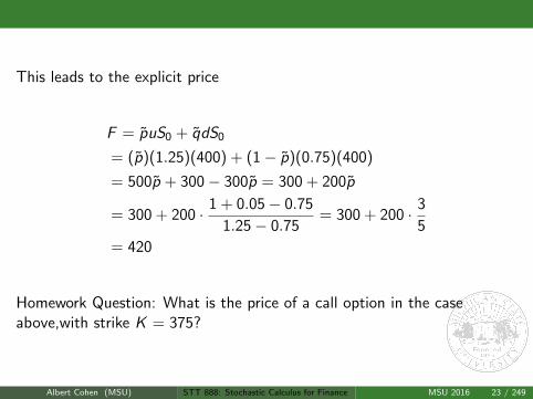
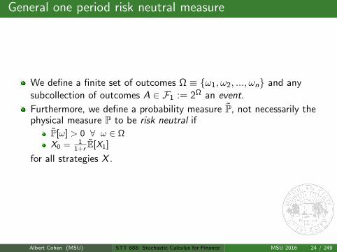
General one period risk neutral measure
We define a finite set of outcomes Ω ≡ ω1, ω2, ..., ωn and anysubcollection of outcomes A ∈ F1 := 2Ω an event.
Furthermore, we define a probability measure P, not necessarily thephysical measure P to be risk neutral if
P[ω] > 0 ∀ ω ∈ ΩX0 = 1
1+r E[X1]
for all strategies X .
Albert Cohen (MSU) STT 888: Stochastic Calculus for Finance MSU 2016 24 / 249
General one period risk neutral measure
The measure is indifferent to investing in a zero-coupon bond, or arisky asset X
The same initial capital X0 in both cases produces the same”‘average”’ return after one period.
Not the physical measure attached by observation, experts, etc..
In fact, physical measure has no impact on pricing
Albert Cohen (MSU) STT 888: Stochastic Calculus for Finance MSU 2016 25 / 249

Example: Risk Neutral measure for trinomial case
Assume that Ω = ω1, ω2, ω3 with
S1(ω1) = uS0
S1(ω2) = S0
S1(ω3) = dS0
Given a payoff V1(ω) to replicate, are we assured that a replicatingstrategy exists?
Albert Cohen (MSU) STT 888: Stochastic Calculus for Finance MSU 2016 26 / 249
Example: Risk Neutral measure for trinomial case
Assume that Ω = ω1, ω2, ω3 with
S1(ω1) = uS0
S1(ω2) = S0
S1(ω3) = dS0
Given a payoff V1(ω) to replicate, are we assured that a replicatingstrategy exists?
Albert Cohen (MSU) STT 888: Stochastic Calculus for Finance MSU 2016 26 / 249
Example: Risk Neutral measure for trinomial case
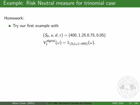
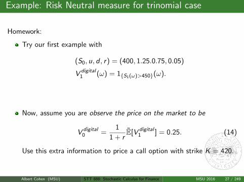
Homework:
Try our first example with
(S0, u, d , r) = (400, 1.25.0.75, 0.05)
V digital1 (ω) = 1S1(ω)>450(ω).
Now, assume you are observe the price on the market to be
V digital0 =
1
1 + rE[V digital
1 ] = 0.25. (14)
Use this extra information to price a call option with strike K = 420.
Albert Cohen (MSU) STT 888: Stochastic Calculus for Finance MSU 2016 27 / 249
Example: Risk Neutral measure for trinomial case
Homework:
Try our first example with
(S0, u, d , r) = (400, 1.25.0.75, 0.05)
V digital1 (ω) = 1S1(ω)>450(ω).
Now, assume you are observe the price on the market to be
V digital0 =
1
1 + rE[V digital
1 ] = 0.25. (14)
Use this extra information to price a call option with strike K = 420.
Albert Cohen (MSU) STT 888: Stochastic Calculus for Finance MSU 2016 27 / 249
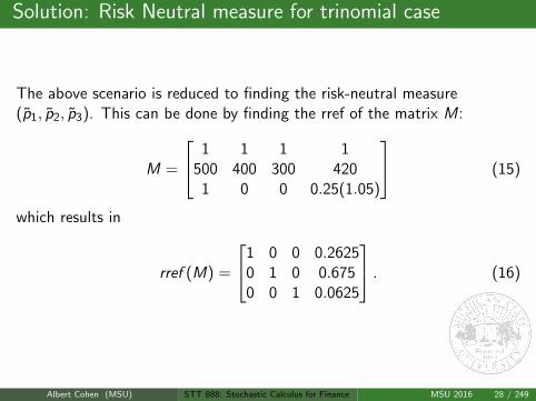
Solution: Risk Neutral measure for trinomial case
The above scenario is reduced to finding the risk-neutral measure(p1, p2, p3). This can be done by finding the rref of the matrix M:
M =
1 1 1 1500 400 300 420
1 0 0 0.25(1.05)
(15)
which results in
rref (M) =
1 0 0 0.26250 1 0 0.6750 0 1 0.0625
. (16)
Albert Cohen (MSU) STT 888: Stochastic Calculus for Finance MSU 2016 28 / 249
Solution: Risk Neutral measure for trinomial case
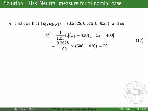
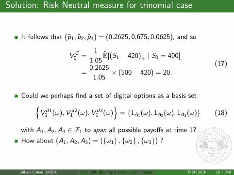
It follows that (p1, p2, p3) = (0.2625, 0.675, 0.0625), and so
V C0 =
1
1.05E[(S1 − 420)+ | S0 = 400]
=0.2625
1.05× (500− 420) = 20.
(17)
Could we perhaps find a set of digital options as a basis setV d1
1 (ω),V d21 (ω),V d3
1 (ω)
= 1A1(ω), 1A2(ω), 1A3(ω) (18)
with A1,A2,A3 ∈ F1 to span all possible payoffs at time 1?
How about (A1,A2,A3) = (ω1 , ω2 , ω3) ?
Albert Cohen (MSU) STT 888: Stochastic Calculus for Finance MSU 2016 29 / 249
Solution: Risk Neutral measure for trinomial case
It follows that (p1, p2, p3) = (0.2625, 0.675, 0.0625), and so
V C0 =
1
1.05E[(S1 − 420)+ | S0 = 400]
=0.2625
1.05× (500− 420) = 20.
(17)
Could we perhaps find a set of digital options as a basis setV d1
1 (ω),V d21 (ω),V d3
1 (ω)
= 1A1(ω), 1A2(ω), 1A3(ω) (18)
with A1,A2,A3 ∈ F1 to span all possible payoffs at time 1?
How about (A1,A2,A3) = (ω1 , ω2 , ω3) ?
Albert Cohen (MSU) STT 888: Stochastic Calculus for Finance MSU 2016 29 / 249
Exchange one stock for another
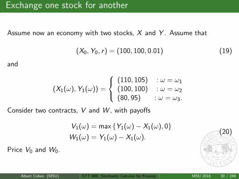
Assume now an economy with two stocks, X and Y . Assume that
(X0,Y0, r) = (100, 100, 0.01) (19)
and
(X1(ω),Y1(ω)) =
(110, 105) : ω = ω1
(100, 100) : ω = ω2
(80, 95) : ω = ω3.
Consider two contracts, V and W , with payoffs
V1(ω) = max Y1(ω)− X1(ω), 0W1(ω) = Y1(ω)− X1(ω).
(20)
Price V0 and W0.
Albert Cohen (MSU) STT 888: Stochastic Calculus for Finance MSU 2016 30 / 249
Exchange one stock for another
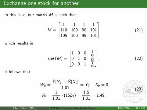
In this case, our matrix M is such that
M =
1 1 1 1110 100 80 101105 100 95 101
(21)
which results in
rref (M) =
1 0 0 310
0 1 0 610
0 0 1 110
. (22)
It follows that
W0 =E[Y1]− E[X1]
1.01= Y0 − X0 = 0
V0 =1
1.01· (15p3) =
1.5
1.01= 1.49.
(23)
Albert Cohen (MSU) STT 888: Stochastic Calculus for Finance MSU 2016 31 / 249
Existence of Risk Neutral measure
Let P be a probability measure on a finite space Ω. The following areequivalent:
P is a risk neutral measure
For all traded securities S i , S i0 = 1
1+r E[S i
1
]Proof: Homework (Hint: One direction is much easier than others. Also,strategies are linear in the underlying asset.)
Albert Cohen (MSU) STT 888: Stochastic Calculus for Finance MSU 2016 32 / 249
Existence of Risk Neutral measure
Let P be a probability measure on a finite space Ω. The following areequivalent:
P is a risk neutral measure
For all traded securities S i , S i0 = 1
1+r E[S i
1
]
Proof: Homework (Hint: One direction is much easier than others. Also,strategies are linear in the underlying asset.)
Albert Cohen (MSU) STT 888: Stochastic Calculus for Finance MSU 2016 32 / 249
Existence of Risk Neutral measure
Let P be a probability measure on a finite space Ω. The following areequivalent:
P is a risk neutral measure
For all traded securities S i , S i0 = 1
1+r E[S i
1
]Proof: Homework (Hint: One direction is much easier than others. Also,strategies are linear in the underlying asset.)
Albert Cohen (MSU) STT 888: Stochastic Calculus for Finance MSU 2016 32 / 249
Complete Markets
A market is complete if it is arbitrage free and every non-traded asset canbe replicated.
Fundamental Theorem of Asset Pricing 1: A market is arbitrage freeiff there exists a risk neutral measure
Fundamental Theorem of Asset Pricing 2: A market is complete iffthere exists exactly one risk neutral measure
Proof(s): We will go over these in detail later!
Albert Cohen (MSU) STT 888: Stochastic Calculus for Finance MSU 2016 33 / 249
Optimal Investment for a Strictly Risk Averse Investor
Assume a complete market, with a unique risk-neutral measure P.
Characterize an investor by her pair (x ,U) of initial capital x ∈ X andutility function U : X → R+.
Assume U ′(x) > 0.
Assume U ′′(x) < 0.
Define the Radon-Nikodym derivative of P to P as the randomvariable
Z (ω) :=P(ω)
P(ω). (24)
Note that Z is used to map expectations under P to expectationsunder P: For any random variable X , it follows that
E[X ] = E[ZX ]. (25)
Albert Cohen (MSU) STT 888: Stochastic Calculus for Finance MSU 2016 34 / 249
Optimal Investment for a Strictly Risk Averse Investor
A strictly risk-averse investor now wishes to maximize her expected utilityof a portfolio at time 1, given initial capital at time 0:
u(x) := maxX1∈Ax
E[U(X1)]
Ax := all portfolio values at time 1 with initial capital x .(26)
Albert Cohen (MSU) STT 888: Stochastic Calculus for Finance MSU 2016 35 / 249
Optimal Investment for a Strictly Risk Averse Investor
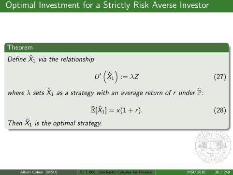
Theorem
Define X1 via the relationship
U ′(
X1
):= λZ (27)
where λ sets X1 as a strategy with an average return of r under P:
E[X1] = x(1 + r). (28)
Then X1 is the optimal strategy.
Albert Cohen (MSU) STT 888: Stochastic Calculus for Finance MSU 2016 36 / 249
Optimal Investment for a Strictly Risk Averse Investor
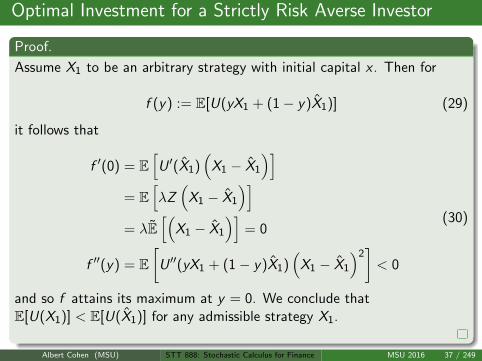
Proof.
Assume X1 to be an arbitrary strategy with initial capital x . Then for
f (y) := E[U(yX1 + (1− y)X1)] (29)
it follows that
f ′(0) = E[U ′(X1)
(X1 − X1
)]= E
[λZ(
X1 − X1
)]= λE
[(X1 − X1
)]= 0
f ′′(y) = E[
U ′′(yX1 + (1− y)X1)(
X1 − X1
)2]< 0
(30)
and so f attains its maximum at y = 0. We conclude thatE[U(X1)] < E[U(X1)] for any admissible strategy X1.
Albert Cohen (MSU) STT 888: Stochastic Calculus for Finance MSU 2016 37 / 249
Optimal Investment: Example
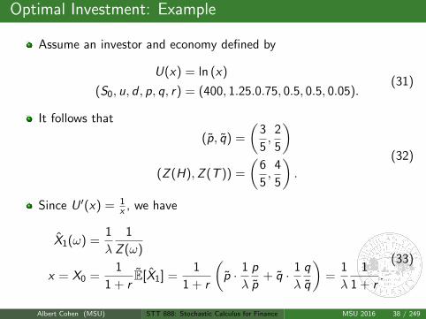
Assume an investor and economy defined by
U(x) = ln (x)
(S0, u, d , p, q, r) = (400, 1.25.0.75, 0.5, 0.5, 0.05).(31)
It follows that
(p, q) =
(3
5,
2
5
)(Z (H),Z (T )) =
(6
5,
4
5
).
(32)
Since U ′(x) = 1x , we have
X1(ω) =1
λ
1
Z (ω)
x = X0 =1
1 + rE[X1] =
1
1 + r
(p · 1
λ
p
p+ q · 1
λ
q
q
)=
1
λ
1
1 + r.
(33)
Albert Cohen (MSU) STT 888: Stochastic Calculus for Finance MSU 2016 38 / 249
Optimal Investment: Example
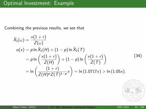
Combining the previous results, we see that
X1(ω) =x(1 + r)
Z (ω)
u(x) = p ln X1(H) + (1− p) ln X1(T )
= p ln
(x(1 + r)
Z (H)
)+ (1− p) ln
(x(1 + r)
Z (T )
)= ln
((1 + r)
Z (H)pZ (T )1−p x
)= ln (1.0717x) > ln (1.05x).
(34)
Albert Cohen (MSU) STT 888: Stochastic Calculus for Finance MSU 2016 39 / 249
Optimal Investment: Example
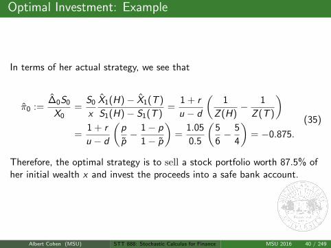
In terms of her actual strategy, we see that
π0 :=∆0S0
X0=
S0
x
X1(H)− X1(T )
S1(H)− S1(T )=
1 + r
u − d
(1
Z (H)− 1
Z (T )
)=
1 + r
u − d
(p
p− 1− p
1− p
)=
1.05
0.5
(5
6− 5
4
)= −0.875.
(35)
Therefore, the optimal strategy is to sell a stock portfolio worth 87.5% ofher initial wealth x and invest the proceeds into a safe bank account.
Albert Cohen (MSU) STT 888: Stochastic Calculus for Finance MSU 2016 40 / 249
Optimal Investment: Example
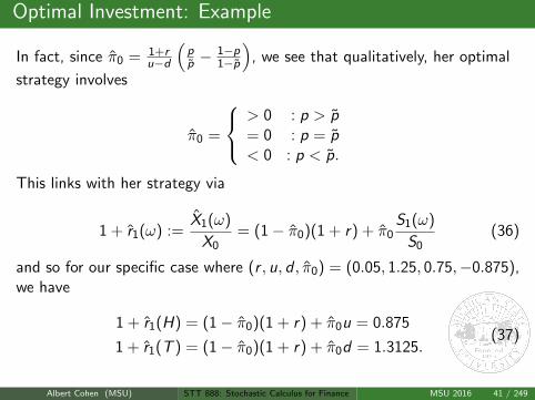
In fact, since π0 = 1+ru−d
(pp −
1−p1−p
), we see that qualitatively, her optimal
strategy involves
π0 =
> 0 : p > p= 0 : p = p< 0 : p < p.
This links with her strategy via
1 + r1(ω) :=X1(ω)
X0= (1− π0)(1 + r) + π0
S1(ω)
S0(36)
and so for our specific case where (r , u, d , π0) = (0.05, 1.25, 0.75,−0.875),we have
1 + r1(H) = (1− π0)(1 + r) + π0u = 0.875
1 + r1(T ) = (1− π0)(1 + r) + π0d = 1.3125.(37)
Albert Cohen (MSU) STT 888: Stochastic Calculus for Finance MSU 2016 41 / 249
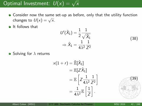
Optimal Investment: U(x) =√x
Consider now the same set-up as before, only that the utility functionchanges to U(x) =
√x .
It follows that
U ′(X1) =1
2
1√X1
⇒ X1 =1
4λ2
1
Z 2
(38)
Solving for λ returns
x(1 + r) = E[X1]
= E[Z X1]
= E[
Z1
4λ2
1
Z 2
]=
1
4λ2E[
1
Z
].
(39)
Albert Cohen (MSU) STT 888: Stochastic Calculus for Finance MSU 2016 42 / 249
Optimal Investment: U(x) =√x
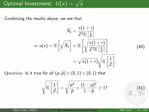
Combining the results above, we see that
X1 =x(1 + r)
Z 2E[
1Z
]⇒ u(x) = E
[√X1
]= E
[√x(1 + r)
Z 2E[
1Z
]]
=√
x(1 + r)
√E[
1
Z
].
(40)
Question: Is it true for all (p, p) ∈ (0, 1)× (0, 1) that√E[
1
Z
]=
√p2
p+
(1− p)2
1− p≥ 1? (41)
Albert Cohen (MSU) STT 888: Stochastic Calculus for Finance MSU 2016 43 / 249
Optimal Betting at the Omega Horse Track!
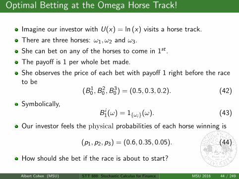
Imagine our investor with U(x) = ln (x) visits a horse track.
There are three horses: ω1, ω2 and ω3.
She can bet on any of the horses to come in 1st .
The payoff is 1 per whole bet made.
She observes the price of each bet with payoff 1 right before the raceto be
(B10 ,B
20 ,B
30 ) = (0.5, 0.3, 0.2). (42)
Symbolically,B i
1(ω) = 1ωi(ω). (43)
Our investor feels the physical probabilities of each horse winning is
(p1, p2, p3) = (0.6, 0.35, 0.05). (44)
How should she bet if the race is about to start?
Albert Cohen (MSU) STT 888: Stochastic Calculus for Finance MSU 2016 44 / 249
Optimal Betting at the Omega Horse Track!
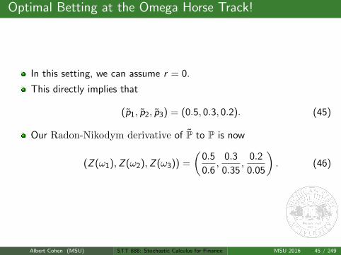
In this setting, we can assume r = 0.
This directly implies that
(p1, p2, p3) = (0.5, 0.3, 0.2). (45)
Our Radon-Nikodym derivative of P to P is now
(Z (ω1),Z (ω2),Z (ω3)) =
(0.5
0.6,
0.3
0.35,
0.2
0.05
). (46)
Albert Cohen (MSU) STT 888: Stochastic Calculus for Finance MSU 2016 45 / 249
Optimal Betting at the Omega Horse Track!
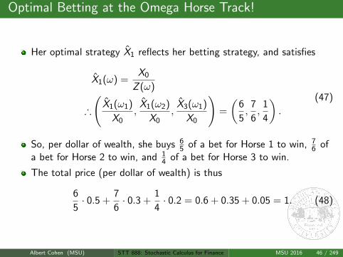
Her optimal strategy X1 reflects her betting strategy, and satisfies
X1(ω) =X0
Z (ω)
∴
(X1(ω1)
X0,
X1(ω2)
X0,
X3(ω1)
X0
)=
(6
5,
7
6,
1
4
).
(47)
So, per dollar of wealth, she buys 65 of a bet for Horse 1 to win, 7
6 ofa bet for Horse 2 to win, and 1
4 of a bet for Horse 3 to win.
The total price (per dollar of wealth) is thus
6
5· 0.5 +
7
6· 0.3 +
1
4· 0.2 = 0.6 + 0.35 + 0.05 = 1. (48)
Albert Cohen (MSU) STT 888: Stochastic Calculus for Finance MSU 2016 46 / 249
Dividends
What about dividends? How do they affect the risk neutral pricing ofexchange and non-exchange traded assets? What if they are paid atdiscrete times? Continuously paid?
Recall that if dividends are paid continuously at rate δ, then 1 share attime 0 will accumulate to eδT shares upon reinvestment of dividends intothe stock until time T .
It follows that to deliver one share of stock S with initial price S0 at timeT , only e−δT shares are needed. Correspondingly,
Fprepaid = e−δTS0
F = erT e−δTS0 = e(r−δ)TS0.(49)
Albert Cohen (MSU) STT 888: Stochastic Calculus for Finance MSU 2016 47 / 249
Dividends
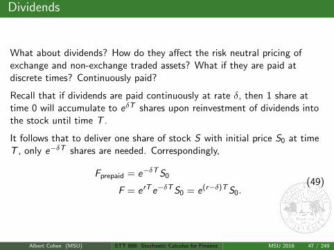
What about dividends? How do they affect the risk neutral pricing ofexchange and non-exchange traded assets? What if they are paid atdiscrete times? Continuously paid?
Recall that if dividends are paid continuously at rate δ, then 1 share attime 0 will accumulate to eδT shares upon reinvestment of dividends intothe stock until time T .
It follows that to deliver one share of stock S with initial price S0 at timeT , only e−δT shares are needed. Correspondingly,
Fprepaid = e−δTS0
F = erT e−δTS0 = e(r−δ)TS0.(49)
Albert Cohen (MSU) STT 888: Stochastic Calculus for Finance MSU 2016 47 / 249
Binomial Option Pricing w/ cts Dividends and Interest
Over a period of length h, interest increases the value of a bond by afactor erh and dividends the value of a stock by a factor of eδh.
Once again, we compute pathwise,
V1(H) = (X0 −∆0S0)erh + ∆0eδhuS0
V1(T ) = (X0 −∆0S0)erh + ∆0eδhdS0
and this results in the modified quantities
∆0 = e−δhV1(H)− V1(T )
(u − d)S0
p =e(r−δ)h − d
u − d
q =u − e(r−δ)h
u − d
Albert Cohen (MSU) STT 888: Stochastic Calculus for Finance MSU 2016 48 / 249
Binomial Option Pricing w/ cts Dividends and Interest
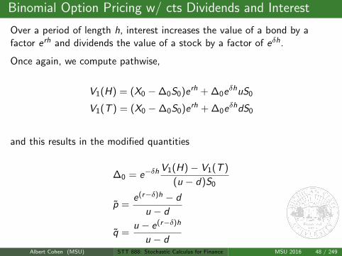
Over a period of length h, interest increases the value of a bond by afactor erh and dividends the value of a stock by a factor of eδh.
Once again, we compute pathwise,
V1(H) = (X0 −∆0S0)erh + ∆0eδhuS0
V1(T ) = (X0 −∆0S0)erh + ∆0eδhdS0
and this results in the modified quantities
∆0 = e−δhV1(H)− V1(T )
(u − d)S0
p =e(r−δ)h − d
u − d
q =u − e(r−δ)h
u − dAlbert Cohen (MSU) STT 888: Stochastic Calculus for Finance MSU 2016 48 / 249
Binomial Models w/ cts Dividends and Interest
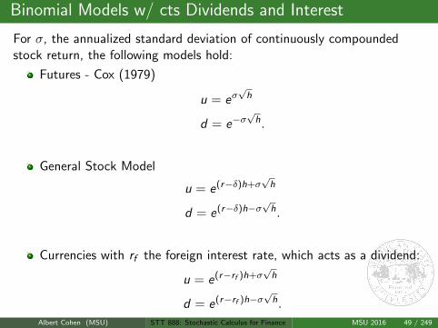
For σ, the annualized standard deviation of continuously compoundedstock return, the following models hold:
Futures - Cox (1979)
u = eσ√h
d = e−σ√h.
General Stock Model
u = e(r−δ)h+σ√h
d = e(r−δ)h−σ√h.
Currencies with rf the foreign interest rate, which acts as a dividend:
u = e(r−rf )h+σ√h
d = e(r−rf )h−σ√h.
Albert Cohen (MSU) STT 888: Stochastic Calculus for Finance MSU 2016 49 / 249
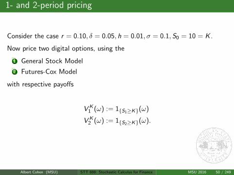
1- and 2-period pricing
Consider the case r = 0.10, δ = 0.05, h = 0.01, σ = 0.1,S0 = 10 = K .
Now price two digital options, using the
1 General Stock Model
2 Futures-Cox Model
with respective payoffs
V K1 (ω) := 1S1≥K(ω)
V K2 (ω) := 1S2≥K(ω).
Albert Cohen (MSU) STT 888: Stochastic Calculus for Finance MSU 2016 50 / 249
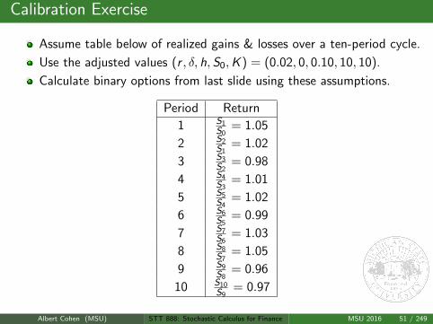
Calibration Exercise
Assume table below of realized gains & losses over a ten-period cycle.
Use the adjusted values (r , δ, h,S0,K ) = (0.02, 0, 0.10, 10, 10).
Calculate binary options from last slide using these assumptions.
Period Return
1 S1S0
= 1.05
2 S2S1
= 1.02
3 S3S2
= 0.98
4 S4S3
= 1.01
5 S5S4
= 1.02
6 S6S5
= 0.99
7 S7S6
= 1.03
8 S8S7
= 1.05
9 S9S8
= 0.96
10 S10S9
= 0.97
Albert Cohen (MSU) STT 888: Stochastic Calculus for Finance MSU 2016 51 / 249
Calibration Exercise: Linear Approximation
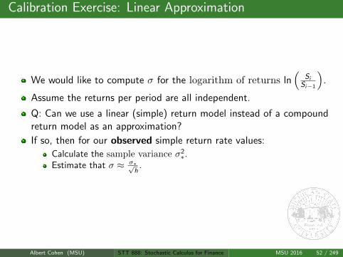
We would like to compute σ for the logarithm of returns ln(
SiSi−1
).
Assume the returns per period are all independent.
Q: Can we use a linear (simple) return model instead of a compoundreturn model as an approximation?
If so, then for our observed simple return rate values:
Calculate the sample variance σ2∗.
Estimate that σ ≈ σ∗√h
.
Albert Cohen (MSU) STT 888: Stochastic Calculus for Finance MSU 2016 52 / 249
Calibration Exercise: Linear Approximation
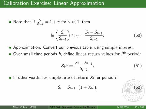
Note that if SiSi−1
= 1 + γ for γ 1, then
ln
(Si
Si−1
)≈ γ =
Si − Si−1
Si−1. (50)
Approximation: Convert our previous table, using simple interest.
Over small time periods h, define linear return values for i th period:
Xih :=Si − Si−1
Si−1. (51)
In other words, for simple rate of return Xi for period i :
Si = Si−1 · (1 + Xih). (52)
Albert Cohen (MSU) STT 888: Stochastic Calculus for Finance MSU 2016 53 / 249
Calibration Exercise: Linear Approximation
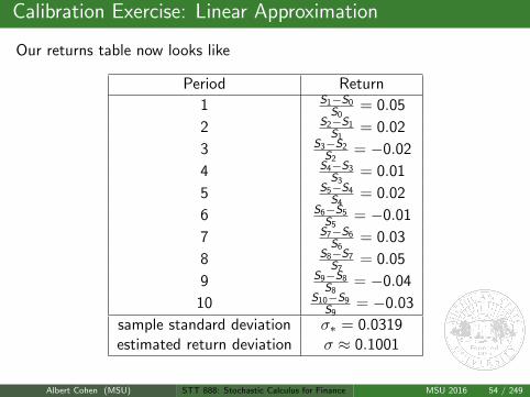
Our returns table now looks like
Period Return
1 S1−S0S0
= 0.05
2 S2−S1S1
= 0.02
3 S3−S2S2
= −0.02
4 S4−S3S3
= 0.01
5 S5−S4S4
= 0.02
6 S6−S5S5
= −0.01
7 S7−S6S6
= 0.03
8 S8−S7S7
= 0.05
9 S9−S8S8
= −0.04
10 S10−S9S9
= −0.03
sample standard deviation σ∗ = 0.0319estimated return deviation σ ≈ 0.1001
Albert Cohen (MSU) STT 888: Stochastic Calculus for Finance MSU 2016 54 / 249
Calibration Exercise: Linear Approximation
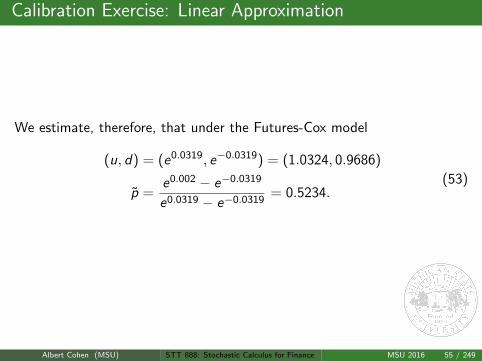
We estimate, therefore, that under the Futures-Cox model
(u, d) = (e0.0319, e−0.0319) = (1.0324, 0.9686)
p =e0.002 − e−0.0319
e0.0319 − e−0.0319= 0.5234.
(53)
Albert Cohen (MSU) STT 888: Stochastic Calculus for Finance MSU 2016 55 / 249
Calibration Exercise: Linear Approximation
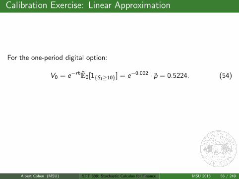
For the one-period digital option:
V0 = e−rhE0[1S1≥10] = e−0.002 · p = 0.5224. (54)
For the two-period digital option:
V0 = e−2rhE0[1S2≥10] = e−0.004 ·[p2 + 2pq
]= 0.7698. (55)
Albert Cohen (MSU) STT 888: Stochastic Calculus for Finance MSU 2016 56 / 249
Calibration Exercise: Linear Approximation
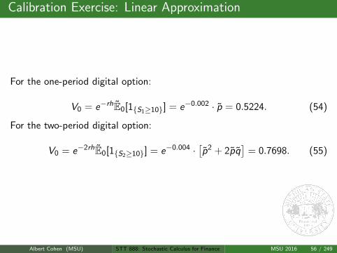
For the one-period digital option:
V0 = e−rhE0[1S1≥10] = e−0.002 · p = 0.5224. (54)
For the two-period digital option:
V0 = e−2rhE0[1S2≥10] = e−0.004 ·[p2 + 2pq
]= 0.7698. (55)
Albert Cohen (MSU) STT 888: Stochastic Calculus for Finance MSU 2016 56 / 249
Calibration Exercise: No Approximation
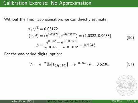
Without the linear approximation, we can directly estimate
σY√
h = 0.03172
(u, d) = (e0.03172, e−0.03172) = (1.0322, 0.9688)
p =e0.002 − e−0.03172
e0.03172 − e−0.03172= 0.5246.
(56)
For the one-period digital option:
V0 = e−rhE0[1S1≥10] = e−0.002 · p = 0.5236. (57)
For the two-period digital option:
V0 = e−2rhE0[1S2≥10] = e−0.004 ·[p2 + 2pq
]= 0.7721. (58)
Albert Cohen (MSU) STT 888: Stochastic Calculus for Finance MSU 2016 57 / 249
Calibration Exercise: No Approximation
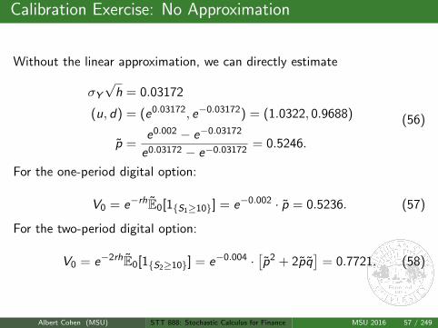
Without the linear approximation, we can directly estimate
σY√
h = 0.03172
(u, d) = (e0.03172, e−0.03172) = (1.0322, 0.9688)
p =e0.002 − e−0.03172
e0.03172 − e−0.03172= 0.5246.
(56)
For the one-period digital option:
V0 = e−rhE0[1S1≥10] = e−0.002 · p = 0.5236. (57)
For the two-period digital option:
V0 = e−2rhE0[1S2≥10] = e−0.004 ·[p2 + 2pq
]= 0.7721. (58)
Albert Cohen (MSU) STT 888: Stochastic Calculus for Finance MSU 2016 57 / 249
1- and 2-period pricing
We can solve for 2-period problems
on a case-by-case basis, or
by developing a general theory for multi-period asset pricing.
In the latter method, we need a general framework to carry out ourcomputations
Albert Cohen (MSU) STT 888: Stochastic Calculus for Finance MSU 2016 58 / 249
Risk Neutral Pricing Formula
Assume now that we have the ”regular assumptions” on our coin flipspace, and that at time N we are asked to deliver a path dependentderivative value VN . Then for times 0 ≤ n ≤ N, the value of thisderivative is computed via
Vn = e−rhEn [Vn+1] (59)
and so
X0 = E0 [XN ]
Xn :=Vn
enh.
(60)
Albert Cohen (MSU) STT 888: Stochastic Calculus for Finance MSU 2016 59 / 249
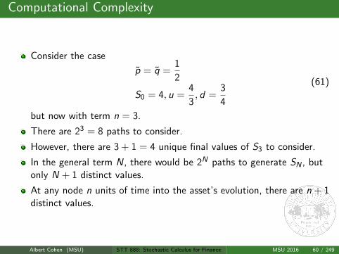
Computational Complexity
Consider the case
p = q =1
2
S0 = 4, u =4
3, d =
3
4
(61)
but now with term n = 3.
There are 23 = 8 paths to consider.
However, there are 3 + 1 = 4 unique final values of S3 to consider.
In the general term N, there would be 2N paths to generate SN , butonly N + 1 distinct values.
At any node n units of time into the asset’s evolution, there are n + 1distinct values.
Albert Cohen (MSU) STT 888: Stochastic Calculus for Finance MSU 2016 60 / 249
Computational Complexity
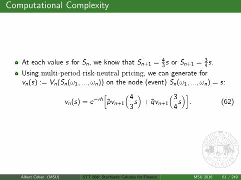
At each value s for Sn, we know that Sn+1 = 43 s or Sn+1 = 3
4 s.
Using multi-period risk-neutral pricing, we can generate forvn(s) := Vn(Sn(ω1, ..., ωn)) on the node (event) Sn(ω1, ..., ωn) = s:
vn(s) = e−rh[pvn+1
(4
3s)
+ qvn+1
(3
4s)]. (62)
Albert Cohen (MSU) STT 888: Stochastic Calculus for Finance MSU 2016 61 / 249
An Example:
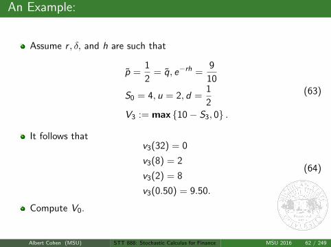
Assume r , δ, and h are such that
p =1
2= q, e−rh =
9
10
S0 = 4, u = 2, d =1
2V3 := max 10− S3, 0 .
(63)
It follows thatv3(32) = 0
v3(8) = 2
v3(2) = 8
v3(0.50) = 9.50.
(64)
Compute V0.
Albert Cohen (MSU) STT 888: Stochastic Calculus for Finance MSU 2016 62 / 249
Markov Processes
If we use the above approach for a more exotic option, say a lookbackoption that pays the maximum over the term of a stock, then we findthis approach lacking.
There is not enough information in the tree or the distinct values forS3 as stated. We need more.
Consider our general multi-period binomial model under P.
Definition We say that a process X is adapted if it depends only on thesequence of flips ω := (ω1, ..., ωn)
Definition We say that an adapted process X is Markov if for every0 ≤ n ≤ N − 1 and every function f (x) there exists another function g(x)such that
En [f (Xn+1)] = g(Xn). (65)
Albert Cohen (MSU) STT 888: Stochastic Calculus for Finance MSU 2016 63 / 249
Markov Processes
This notion of Markovity is essential to our state-dependent pricingalgorithm.
Indeed, our stock process evolves from time n to time n + 1, usingonly the information in Sn.
We can in fact say that for every f (s) there exists a g(s) such that
g(s) = En [f (Sn+1) | Sn = s] . (66)
In fact, that g depends on f :
g(s) = e−rh[pf(4
3s)
+ qf(3
4s)]. (67)
So, for any f (s) := VN(s), we can work our recursive algorithmbackwards to find the gn(s) := Vn(s) for all 0 ≤ n ≤ N − 1
Albert Cohen (MSU) STT 888: Stochastic Calculus for Finance MSU 2016 64 / 249
Markov Processes
Some more thoughts on Markovity:
Consider the example of a Lookback Option.
Here, the payoff is dependent on the realized maximumMn := max0≤i≤nSi of the asset.
Mn is not Markov by itself, but the two-factor process (Mn, Sn) is.Why?
Let’s generate the tree!
Homework Can you think of any other processes that are not Markov?
Albert Cohen (MSU) STT 888: Stochastic Calculus for Finance MSU 2016 65 / 249
Call Options on Zero-Coupon Bonds
Assume an economy where
One period is one year
The one year short term interest rate from time n to time n + 1 is rn.
The rate evolves via a stochastic process:
r0 = 0.02
rn+1 = Xrn
P[X = 2k ] =1
3for k ∈ −1, 0, 1 .
(68)
Albert Cohen (MSU) STT 888: Stochastic Calculus for Finance MSU 2016 66 / 249
Call Options on Zero-Coupon Bonds
Consider now a zero-coupon bond that matures in 3−years withcommon face and redemption value F = 100.
Also consider a call option on this bond that expires in 2−years withstrike K = 97.
Denote Bn and Cn as the bond and call option values, respectively.
Note that we iterate backwards from the values
B3(r) = 100
C2(r) = max B2(r)− 97, 0 .(69)
Compute (B0,C0).
Albert Cohen (MSU) STT 888: Stochastic Calculus for Finance MSU 2016 67 / 249
Call Options on Zero-Coupon Bonds
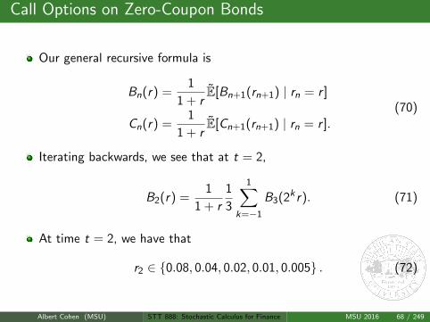
Our general recursive formula is
Bn(r) =1
1 + rE[Bn+1(rn+1) | rn = r ]
Cn(r) =1
1 + rE[Cn+1(rn+1) | rn = r ].
(70)
Iterating backwards, we see that at t = 2,
B2(r) =1
1 + r
1
3
1∑k=−1
B3(2k r). (71)
At time t = 2, we have that
r2 ∈ 0.08, 0.04, 0.02, 0.01, 0.005 . (72)
Albert Cohen (MSU) STT 888: Stochastic Calculus for Finance MSU 2016 68 / 249
Call Options on Zero-Coupon Bonds
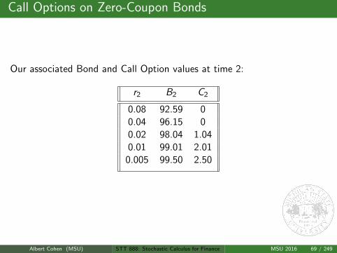
Our associated Bond and Call Option values at time 2:
r2 B2 C2
0.08 92.59 00.04 96.15 00.02 98.04 1.040.01 99.01 2.01
0.005 99.50 2.50
Albert Cohen (MSU) STT 888: Stochastic Calculus for Finance MSU 2016 69 / 249
Call Options on Zero-Coupon Bonds
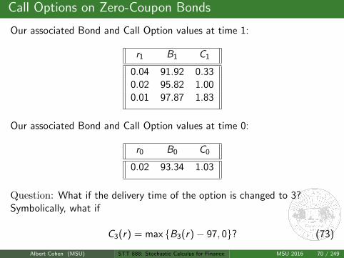
Our associated Bond and Call Option values at time 1:
r1 B1 C1
0.04 91.92 0.330.02 95.82 1.000.01 97.87 1.83
Our associated Bond and Call Option values at time 0:
r0 B0 C0
0.02 93.34 1.03
Question: What if the delivery time of the option is changed to 3?Symbolically, what if
C3(r) = max B3(r)− 97, 0? (73)
Albert Cohen (MSU) STT 888: Stochastic Calculus for Finance MSU 2016 70 / 249
Capital Structure Model
As an analyst for an investments firm, you are tasked with advisingwhether a company’s stock and/or bonds are over/under-priced.
You receive a quarterly report from this company on it’s return onassets, and have compiled a table for the last ten quarters below.
Today, just after the last quarter’s report was issued, you see that inbillions of USD, the value of the company’s assets is 10.
There are presently one billions shares of this company that are beingtraded.
The company does not pay any dividends.
Six months from now, the company is required to pay off a billionzero-coupon bonds. Each bond has a face value of 9.5.
Albert Cohen (MSU) STT 888: Stochastic Calculus for Finance MSU 2016 71 / 249
Capital Structure Model
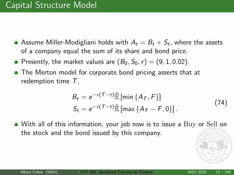
Assume Miller-Modigliani holds with At = Bt + St , where the assetsof a company equal the sum of its share and bond price.
Presently, the market values are (B0, S0, r) = (9, 1, 0.02).
The Merton model for corporate bond pricing asserts that atredemption time T ,
Bt = e−r(T−t)E [min AT ,F]St = e−r(T−t)E [max AT − F , 0] .
(74)
With all of this information, your job now is to issue a Buy or Sell onthe stock and the bond issued by this company.
Albert Cohen (MSU) STT 888: Stochastic Calculus for Finance MSU 2016 72 / 249
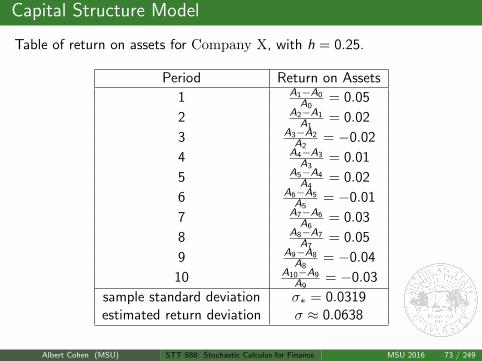
Capital Structure Model
Table of return on assets for Company X, with h = 0.25.
Period Return on Assets
1 A1−A0A0
= 0.05
2 A2−A1A1
= 0.02
3 A3−A2A2
= −0.02
4 A4−A3A3
= 0.01
5 A5−A4A4
= 0.02
6 A6−A5A5
= −0.01
7 A7−A6A6
= 0.03
8 A8−A7A7
= 0.05
9 A9−A8A8
= −0.04
10 A10−A9A9
= −0.03
sample standard deviation σ∗ = 0.0319estimated return deviation σ ≈ 0.0638
Albert Cohen (MSU) STT 888: Stochastic Calculus for Finance MSU 2016 73 / 249
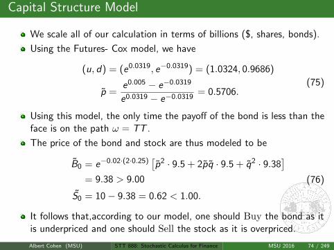
Capital Structure Model
We scale all of our calculation in terms of billions ($, shares, bonds).
Using the Futures- Cox model, we have
(u, d) = (e0.0319, e−0.0319) = (1.0324, 0.9686)
p =e0.005 − e−0.0319
e0.0319 − e−0.0319= 0.5706.
(75)
Using this model, the only time the payoff of the bond is less than theface is on the path ω = TT .
The price of the bond and stock are thus modeled to be
B0 = e−0.02·(2·0.25)[p2 · 9.5 + 2pq · 9.5 + q2 · 9.38
]= 9.38 > 9.00
S0 = 10− 9.38 = 0.62 < 1.00.
(76)
It follows that,according to our model, one should Buy the bond as itis underpriced and one should Sell the stock as it is overpriced.
Albert Cohen (MSU) STT 888: Stochastic Calculus for Finance MSU 2016 74 / 249
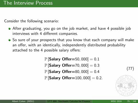
The Interview Process
Consider the following scenario:
After graduating, you go on the job market, and have 4 possible jobinterviews with 4 different companies.
So sure of your prospects that you know that each company will makean offer, with an identically, independently distributed probabilityattached to the 4 possible salary offers:
P [Salary Offer=50, 000] = 0.1
P [Salary Offer=70, 000] = 0.3
P [Salary Offer=80, 000] = 0.4
P [Salary Offer=100, 000] = 0.2.
(77)
Albert Cohen (MSU) STT 888: Stochastic Calculus for Finance MSU 2016 75 / 249

The Interview Process
Questions:
How should you interview?
Specifically, when should you accept an offer and cancel theremaining interviews?
How does your strategy change if you can interview as many times asyou like, but the distribution of offers remains the same as above?
Albert Cohen (MSU) STT 888: Stochastic Calculus for Finance MSU 2016 76 / 249

The Interview Process: Strategy
Some more thoughts...
At any time the student will know only one offer, which she can eitheraccept or reject.
Of course, if the student rejects the first three offers, than she has toaccept the last one.
So, compute the maximal expected salary for the student after thegraduation and the corresponding optimal strategy.
Albert Cohen (MSU) STT 888: Stochastic Calculus for Finance MSU 2016 77 / 249
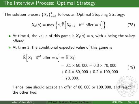
The Interview Process: Optimal Strategy
The solution process Xk4k=1 follows an Optimal Stopping Strategy:
Xk(s) = max
s, E[Xk+1 | kth offer = s
]. (78)
At time 4, the value of this game is X4(s) = s, with s being the salaryoffered.
At time 3, the conditional expected value of this game is
E[X4 | 3rd offer = s
]= E[X4]
= 0.1× 50, 000 + 0.3× 70, 000
+ 0.4× 80, 000 + 0.2× 100, 000
= 78, 000.
(79)
Hence, one should accept an offer of 80, 000 or 100, 000, and rejectthe other two.
Albert Cohen (MSU) STT 888: Stochastic Calculus for Finance MSU 2016 78 / 249
The Interview Process: Optimal Strategy
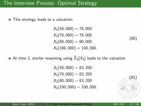
This strategy leads to a valuation:
X3(50, 000) = 78, 000
X3(70, 000) = 78, 000
X3(80, 000) = 80, 000
X3(100, 000) = 100, 000.
(80)
At time 2, similar reasoning using E2[X3] leads to the valuation
X2(50, 000) = 83, 200
X2(70, 000) = 83, 200
X2(80, 000) = 83, 200
X2(100, 000) = 100, 000.
(81)
Albert Cohen (MSU) STT 888: Stochastic Calculus for Finance MSU 2016 79 / 249
The Interview Process: Optimal Strategy
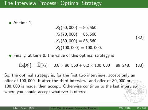
At time 1,X1(50, 000) = 86, 560
X1(70, 000) = 86, 560
X1(80, 000) = 86, 560
X1(100, 000) = 100, 000.
(82)
Finally, at time 0, the value of this optimal strategy is
E0[X1] = E[X1] = 0.8× 86, 560 + 0.2× 100, 000 = 89, 248. (83)
So, the optimal strategy is, for the first two interviews, accept only anoffer of 100, 000. If after the third interview, and offer of 80, 000 or100, 000 is made, then accept. Otherwise continue to the last interviewwhere you should accept whatever is offered.
Albert Cohen (MSU) STT 888: Stochastic Calculus for Finance MSU 2016 80 / 249

Review
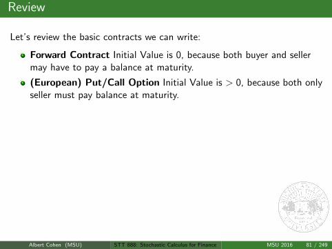
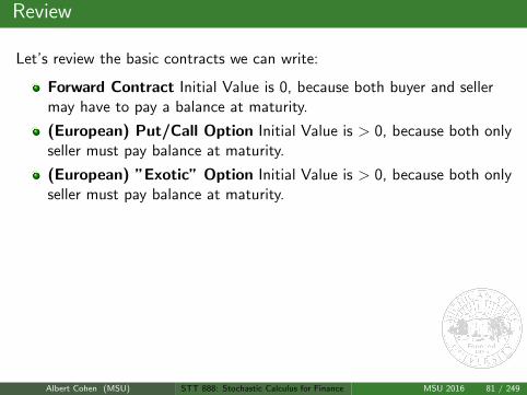
Let’s review the basic contracts we can write:
Forward Contract Initial Value is 0, because both buyer and sellermay have to pay a balance at maturity.
(European) Put/Call Option Initial Value is > 0, because both onlyseller must pay balance at maturity.
(European) ”Exotic” Option Initial Value is > 0, because both onlyseller must pay balance at maturity.
During the term of the contract, can the value of the contract ever fallbelow the intrinsic value of the payoff? Symbolically, does it ever occurthat
vn(s) < g(s) (84)
where g(s) is of the form of g(S) := max S − K , 0, in the case of a Calloption, for example.
Albert Cohen (MSU) STT 888: Stochastic Calculus for Finance MSU 2016 81 / 249

Review
Let’s review the basic contracts we can write:
Forward Contract Initial Value is 0, because both buyer and sellermay have to pay a balance at maturity.
(European) Put/Call Option Initial Value is > 0, because both onlyseller must pay balance at maturity.
(European) ”Exotic” Option Initial Value is > 0, because both onlyseller must pay balance at maturity.
During the term of the contract, can the value of the contract ever fallbelow the intrinsic value of the payoff? Symbolically, does it ever occurthat
vn(s) < g(s) (84)
where g(s) is of the form of g(S) := max S − K , 0, in the case of a Calloption, for example.
Albert Cohen (MSU) STT 888: Stochastic Calculus for Finance MSU 2016 81 / 249
Early Exercise
If σ = 0, and so uncertainty vanishes, then an investor would seek toexercise early if
rK > δS . (85)
If σ > 0, then the situation involves deeper analysis.
Whether solving a free boundary problem or analyzing a binomialtree, it is likely that a computer will be involved in helping theinvestor to determine the optimal exercise time.
Albert Cohen (MSU) STT 888: Stochastic Calculus for Finance MSU 2016 82 / 249

For Freedom! (we must charge extra...)
What happens if we write a contract that allows the purchaser to exercisethe contract whenever she feels it to be in her advantage? By allowing thisextra freedom, we must
Charge more than we would for a European contract that is exercisedonly at the term N.
Hedge our replicating strategy X differently, to allow for thepossibility of early exercise.
Albert Cohen (MSU) STT 888: Stochastic Calculus for Finance MSU 2016 83 / 249
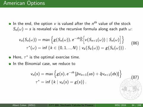
American Options
In the end, the option v is valued after the nth value of the stockSn(ω) = s is revealed via the recursive formula along each path ω:
vn(Sn(ω)) = max
g(Sn(ω)), e−rhE[v(Sn+1(ω)) | Sn(ω)
]τ∗(ω) = inf k ∈ 0, 1, ..,N | vk(Sk(ω)) = g(Sk(ω)) .
(86)
Here, τ∗ is the optimal exercise time.
In the Binomial case, we reduce to
vn(s) = max
g(s), e−rh [pvn+1(us) + qvn+1(ds)]
τ∗ = inf k | vk(s) = g(s) .(87)
Albert Cohen (MSU) STT 888: Stochastic Calculus for Finance MSU 2016 84 / 249
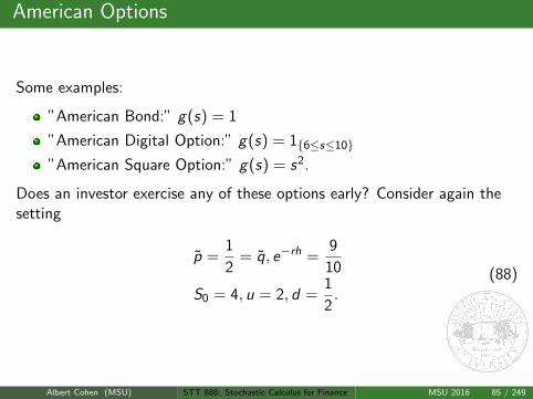
American Options
Some examples:
”American Bond:” g(s) = 1
”American Digital Option:” g(s) = 16≤s≤10
”American Square Option:” g(s) = s2.
Does an investor exercise any of these options early? Consider again thesetting
p =1
2= q, e−rh =
9
10
S0 = 4, u = 2, d =1
2.
(88)
Albert Cohen (MSU) STT 888: Stochastic Calculus for Finance MSU 2016 85 / 249
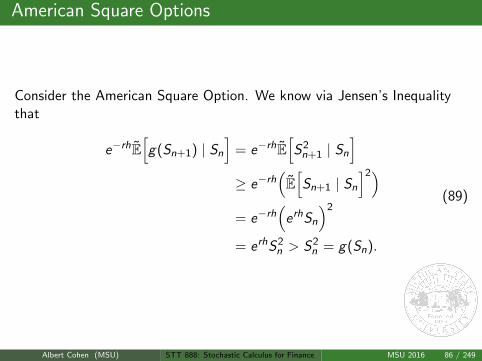
American Square Options
Consider the American Square Option. We know via Jensen’s Inequalitythat
e−rhE[g(Sn+1) | Sn
]= e−rhE
[S2n+1 | Sn
]≥ e−rh
(E[Sn+1 | Sn
]2)= e−rh
(erhSn
)2
= erhS2n > S2
n = g(Sn).
(89)
Albert Cohen (MSU) STT 888: Stochastic Calculus for Finance MSU 2016 86 / 249
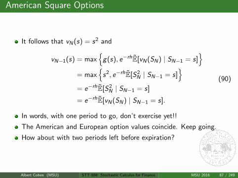
American Square Options
It follows that vN(s) = s2 and
vN−1(s) = max
g(s), e−rhE[vN(SN) | SN−1 = s]
= max
s2, e−rhE[S2N | SN−1 = s]
= e−rhE[S2
N | SN−1 = s]
= e−rhE[vN(SN) | SN−1 = s].
(90)
In words, with one period to go, don’t exercise yet!!
The American and European option values coincide. Keep going.
How about with two periods left before expiration?
Albert Cohen (MSU) STT 888: Stochastic Calculus for Finance MSU 2016 87 / 249
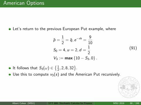
American Options
Let’s return to the previous European Put example, where
p =1
2= q, e−rh =
9
10
S0 = 4, u = 2, d =1
2V3 := max 10− S3, 0 .
(91)
It follows that S3(ω) ∈
12 , 2, 8, 32
.
Use this to compute v3(s) and the American Put recursively.
Albert Cohen (MSU) STT 888: Stochastic Calculus for Finance MSU 2016 88 / 249
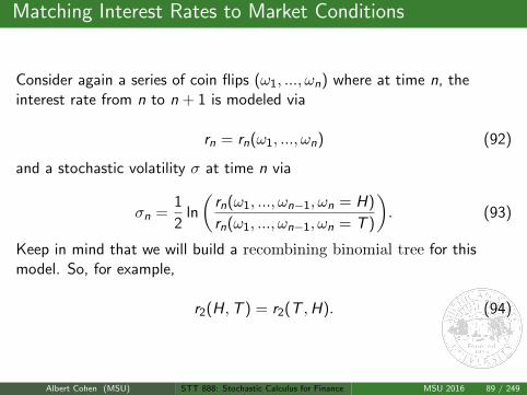
Matching Interest Rates to Market Conditions
Consider again a series of coin flips (ω1, ..., ωn) where at time n, theinterest rate from n to n + 1 is modeled via
rn = rn(ω1, ..., ωn) (92)
and a stochastic volatility σ at time n via
σn =1
2ln
(rn(ω1, ..., ωn−1, ωn = H)
rn(ω1, ..., ωn−1, ωn = T )
). (93)
Keep in mind that we will build a recombining binomial tree for thismodel. So, for example,
r2(H,T ) = r2(T ,H). (94)
Albert Cohen (MSU) STT 888: Stochastic Calculus for Finance MSU 2016 89 / 249
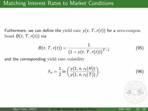
Matching Interest Rates to Market Conditions
Futhermore, we can define the yield rate y(t,T , r(t)) for a zero-couponbond B(t,T , r(t)) via
B(t,T , r(t)) =1
(1 + y(t,T , r(t)))T−t(95)
and the corresponding yield rate volatility
σn =1
2ln
(y(1, n, r1(H))
y(1, n, r1(T ))
). (96)
Albert Cohen (MSU) STT 888: Stochastic Calculus for Finance MSU 2016 90 / 249
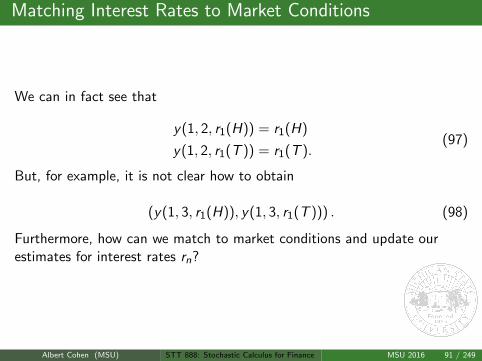
Matching Interest Rates to Market Conditions
We can in fact see that
y(1, 2, r1(H)) = r1(H)
y(1, 2, r1(T )) = r1(T ).(97)
But, for example, it is not clear how to obtain
(y(1, 3, r1(H)), y(1, 3, r1(T ))) . (98)
Furthermore, how can we match to market conditions and update ourestimates for interest rates rn?
Albert Cohen (MSU) STT 888: Stochastic Calculus for Finance MSU 2016 91 / 249
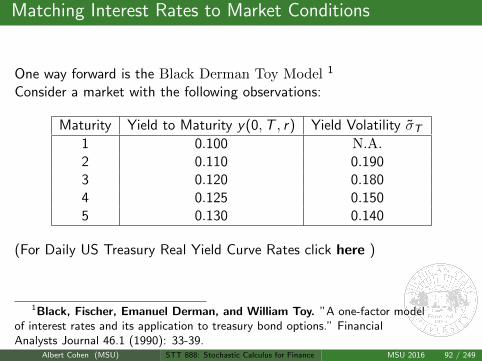
Matching Interest Rates to Market Conditions
One way forward is the Black Derman Toy Model 1
Consider a market with the following observations:
Maturity Yield to Maturity y(0,T , r) Yield Volatility σT1 0.100 N.A.2 0.110 0.1903 0.120 0.1804 0.125 0.1505 0.130 0.140
(For Daily US Treasury Real Yield Curve Rates click here )
1Black, Fischer, Emanuel Derman, and William Toy. ”A one-factor modelof interest rates and its application to treasury bond options.” FinancialAnalysts Journal 46.1 (1990): 33-39.
Albert Cohen (MSU) STT 888: Stochastic Calculus for Finance MSU 2016 92 / 249
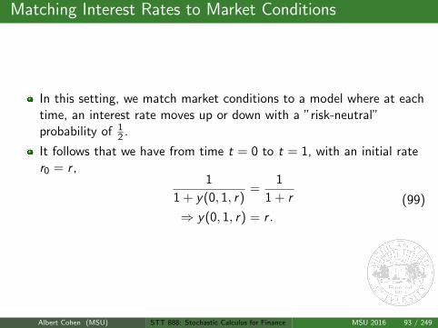
Matching Interest Rates to Market Conditions
In this setting, we match market conditions to a model where at eachtime, an interest rate moves up or down with a ”risk-neutral”probability of 1
2 .
It follows that we have from time t = 0 to t = 1, with an initial rater0 = r ,
1
1 + y(0, 1, r)=
1
1 + r
⇒ y(0, 1, r) = r .
(99)
Albert Cohen (MSU) STT 888: Stochastic Calculus for Finance MSU 2016 93 / 249
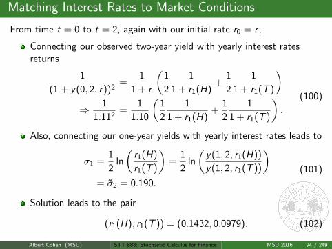
Matching Interest Rates to Market Conditions
From time t = 0 to t = 2, again with our initial rate r0 = r ,
Connecting our observed two-year yield with yearly interest ratesreturns
1
(1 + y(0, 2, r))2=
1
1 + r
(1
2
1
1 + r1(H)+
1
2
1
1 + r1(T )
)⇒ 1
1.112=
1
1.10
(1
2
1
1 + r1(H)+
1
2
1
1 + r1(T )
).
(100)
Also, connecting our one-year yields with yearly interest rates leads to
σ1 =1
2ln
(r1(H)
r1(T )
)=
1
2ln
(y(1, 2, r1(H))
y(1, 2, r1(T ))
)= σ2 = 0.190.
(101)
Solution leads to the pair
(r1(H), r1(T )) = (0.1432, 0.0979). (102)
Albert Cohen (MSU) STT 888: Stochastic Calculus for Finance MSU 2016 94 / 249
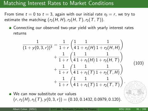
Matching Interest Rates to Market Conditions
From time t = 0 to t = 3, again with our initial rate r0 = r , we try toestimate the matching (r2(H,H), r2(H,T ), r2(T ,T )).
Connecting our observed two-year yield with yearly interest ratesreturns
1
(1 + y(0, 3, r))3=
1
1 + r
(1
4
1
1 + r1(H)
1
1 + r2(H,H)
)+
1
1 + r
(1
4
1
1 + r1(H)
1
1 + r2(H,T )
)+
1
1 + r
(1
4
1
1 + r1(T )
1
1 + r2(T ,H)
)+
1
1 + r
(1
4
1
1 + r1(T )
1
1 + r2(T ,T )
).
(103)
We can now substitute our values(r , r1(H), r1(T ), y(0, 3, r)) = (0.10, 0.1432, 0.0979, 0.120).
Albert Cohen (MSU) STT 888: Stochastic Calculus for Finance MSU 2016 95 / 249
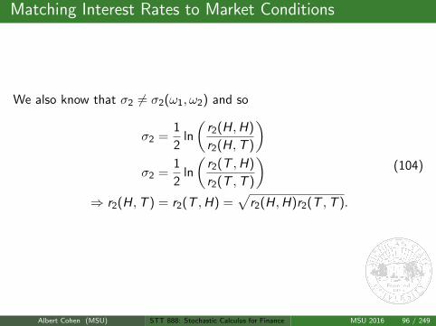
Matching Interest Rates to Market Conditions
We also know that σ2 6= σ2(ω1, ω2) and so
σ2 =1
2ln
(r2(H,H)
r2(H,T )
)σ2 =
1
2ln
(r2(T ,H)
r2(T ,T )
)⇒ r2(H,T ) = r2(T ,H) =
√r2(H,H)r2(T ,T ).
(104)
Albert Cohen (MSU) STT 888: Stochastic Calculus for Finance MSU 2016 96 / 249
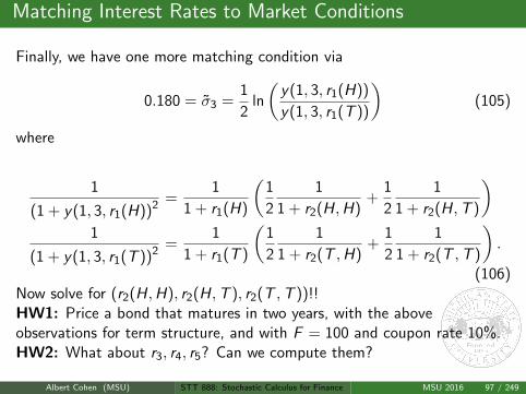
Matching Interest Rates to Market Conditions
Finally, we have one more matching condition via
0.180 = σ3 =1
2ln
(y(1, 3, r1(H))
y(1, 3, r1(T ))
)(105)
where
1
(1 + y(1, 3, r1(H))2=
1
1 + r1(H)
(1
2
1
1 + r2(H,H)+
1
2
1
1 + r2(H,T )
)1
(1 + y(1, 3, r1(T ))2=
1
1 + r1(T )
(1
2
1
1 + r2(T ,H)+
1
2
1
1 + r2(T ,T )
).
(106)Now solve for (r2(H,H), r2(H,T ), r2(T ,T ))!!HW1: Price a bond that matures in two years, with the aboveobservations for term structure, and with F = 100 and coupon rate 10%.HW2: What about r3, r4, r5? Can we compute them?
Albert Cohen (MSU) STT 888: Stochastic Calculus for Finance MSU 2016 97 / 249
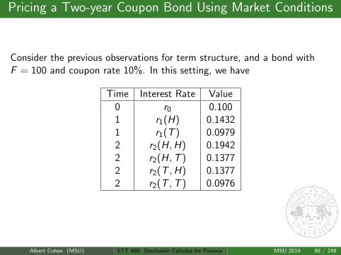
Pricing a Two-year Coupon Bond Using Market Conditions
Consider the previous observations for term structure, and a bond withF = 100 and coupon rate 10%. In this setting, we have
Time Interest Rate Value
0 r0 0.1001 r1(H) 0.14321 r1(T ) 0.09792 r2(H,H) 0.19422 r2(H,T ) 0.13772 r2(T ,H) 0.13772 r2(T ,T ) 0.0976
Albert Cohen (MSU) STT 888: Stochastic Calculus for Finance MSU 2016 98 / 249
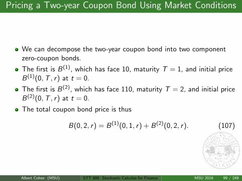
Pricing a Two-year Coupon Bond Using Market Conditions
We can decompose the two-year coupon bond into two componentzero-coupon bonds.
The first is B(1), which has face 10, maturity T = 1, and initial priceB(1)(0,T , r) at t = 0.
The first is B(2), which has face 110, maturity T = 2, and initial priceB(2)(0,T , r) at t = 0.
The total coupon bond price is thus
B(0, 2, r) = B(1)(0, 1, r) + B(2)(0, 2, r). (107)
Albert Cohen (MSU) STT 888: Stochastic Calculus for Finance MSU 2016 99 / 249
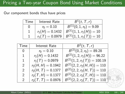
Pricing a Two-year Coupon Bond Using Market Conditions
Our component bonds thus have prices
Time Interest Rate B1(t,T , r)
0 r0 = 0.10 B(1)(0, 1, r0) = 9.09
1 r1(H) = 0.1432 B(1)(1, 1, r1(H)) = 10
1 r1(T ) = 0.0979 B(1)(1, 1, r1(T )) = 10
Time Interest Rate B2(t,T , r)
0 r0 = 0.10 B(2)(0, 2, r0) = 89.28
1 r1(H) = 0.1432 B(2)(1, 2, r1(H)) = 96.22
1 r1(T ) = 0.0979 B(2)(1, 2, r1(T )) = 100.19
2 r2(H,H) = 0.1942 B(2)(2, 2, r2(H,H)) = 110
2 r2(H,T ) = 0.1377 B(2)(2, 2, r2(H,T )) = 110
2 r2(T ,H) = 0.1377 B(2)(2, 2, r2(T ,H)) = 110
2 r2(T ,T ) = 0.0976 B(2)(2, 2, r2(T ,T )) = 110
Albert Cohen (MSU) STT 888: Stochastic Calculus for Finance MSU 2016 100 / 249
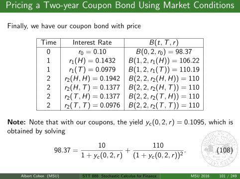
Pricing a Two-year Coupon Bond Using Market Conditions
Finally, we have our coupon bond with price
Time Interest Rate B(t,T , r)
0 r0 = 0.10 B(0, 2, r0) = 98.371 r1(H) = 0.1432 B(1, 2, r1(H)) = 106.221 r1(T ) = 0.0979 B(1, 2, r1(T )) = 110.192 r2(H,H) = 0.1942 B(2, 2, r2(H,H)) = 1102 r2(H,T ) = 0.1377 B(2, 2, r2(H,T )) = 1102 r2(T ,H) = 0.1377 B(2, 2, r2(T ,H)) = 1102 r2(T ,T ) = 0.0976 B(2, 2, r2(T ,T )) = 110
Note: Note that with our coupons, the yield yc(0, 2, r) = 0.1095, which isobtained by solving
98.37 =10
1 + yc(0, 2, r)+
110
(1 + yc(0, 2, r))2. (108)
Albert Cohen (MSU) STT 888: Stochastic Calculus for Finance MSU 2016 101 / 249
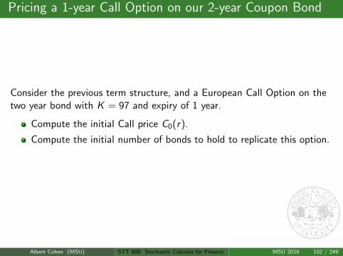
Pricing a 1-year Call Option on our 2-year Coupon Bond
Consider the previous term structure, and a European Call Option on thetwo year bond with K = 97 and expiry of 1 year.
Compute the initial Call price C0(r).
Compute the initial number of bonds to hold to replicate this option.
Albert Cohen (MSU) STT 888: Stochastic Calculus for Finance MSU 2016 102 / 249
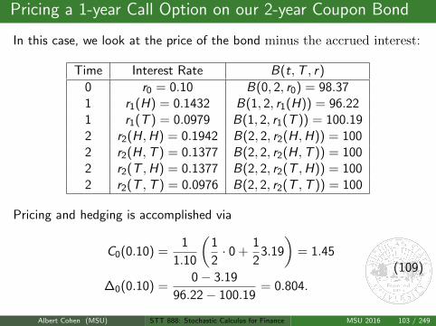
Pricing a 1-year Call Option on our 2-year Coupon Bond
In this case, we look at the price of the bond minus the accrued interest:
Time Interest Rate B(t,T , r)
0 r0 = 0.10 B(0, 2, r0) = 98.371 r1(H) = 0.1432 B(1, 2, r1(H)) = 96.221 r1(T ) = 0.0979 B(1, 2, r1(T )) = 100.192 r2(H,H) = 0.1942 B(2, 2, r2(H,H)) = 1002 r2(H,T ) = 0.1377 B(2, 2, r2(H,T )) = 1002 r2(T ,H) = 0.1377 B(2, 2, r2(T ,H)) = 1002 r2(T ,T ) = 0.0976 B(2, 2, r2(T ,T )) = 100
Pricing and hedging is accomplished via
C0(0.10) =1
1.10
(1
2· 0 +
1
23.19
)= 1.45
∆0(0.10) =0− 3.19
96.22− 100.19= 0.804.
(109)
Albert Cohen (MSU) STT 888: Stochastic Calculus for Finance MSU 2016 103 / 249
Asian Options
In times of high volatility or frequent trading, a company may want toprotect against large price movements over an entire time period, using anaverage. For example, if a company is looking at foreign exchange marketsor markets that may be subject to stock pinning due to large actors.
As an input, the average of an asset is used as an input against a strike,instead of the spot price.
There are two possibilities for the input in the discrete case: h = TN and
Arithmetic Average: IA(T ) := 1N
∑Nk=1 Skh .
Geometric Average: IG (T ) :=(
ΠNk=1Skh
) 1N
.
HW: Is there an ordering for IA, IG that is independent of T ?
Albert Cohen (MSU) STT 888: Stochastic Calculus for Finance MSU 2016 104 / 249
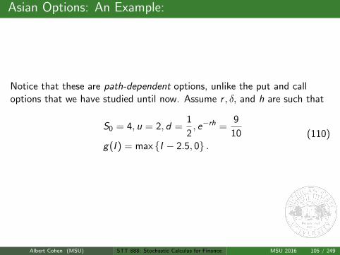
Asian Options: An Example:
Notice that these are path-dependent options, unlike the put and calloptions that we have studied until now. Assume r , δ, and h are such that
S0 = 4, u = 2, d =1
2, e−rh =
9
10g(I ) = max I − 2.5, 0 .
(110)
Albert Cohen (MSU) STT 888: Stochastic Calculus for Finance MSU 2016 105 / 249
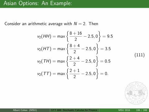
Asian Options: An Example:
Consider an arithmetic average with N = 2. Then
v2(HH) = max
8 + 16
2− 2.5, 0
= 9.5
v2(HT ) = max
8 + 4
2− 2.5, 0
= 3.5
v2(TH) = max
2 + 4
2− 2.5, 0
= 0.5
v2(TT ) = max
2 + 1
2− 2.5, 0
= 0.
(111)
Compute v0, assuming a European structure. How about an Americanstructure?
Albert Cohen (MSU) STT 888: Stochastic Calculus for Finance MSU 2016 106 / 249
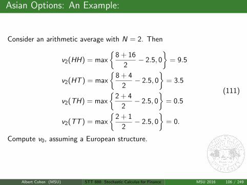
Asian Options: An Example:
Consider an arithmetic average with N = 2. Then
v2(HH) = max
8 + 16
2− 2.5, 0
= 9.5
v2(HT ) = max
8 + 4
2− 2.5, 0
= 3.5
v2(TH) = max
2 + 4
2− 2.5, 0
= 0.5
v2(TT ) = max
2 + 1
2− 2.5, 0
= 0.
(111)
Compute v0, assuming a European structure.
How about an Americanstructure?
Albert Cohen (MSU) STT 888: Stochastic Calculus for Finance MSU 2016 106 / 249
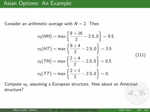
Asian Options: An Example:
Consider an arithmetic average with N = 2. Then
v2(HH) = max
8 + 16
2− 2.5, 0
= 9.5
v2(HT ) = max
8 + 4
2− 2.5, 0
= 3.5
v2(TH) = max
2 + 4
2− 2.5, 0
= 0.5
v2(TT ) = max
2 + 1
2− 2.5, 0
= 0.
(111)
Compute v0, assuming a European structure. How about an Americanstructure?
Albert Cohen (MSU) STT 888: Stochastic Calculus for Finance MSU 2016 106 / 249
Lognormality
Analyzing returns, we assume:
A probability space(
Ω,F ,P).
Our asset St(ω) has an associated return over any period (t, t + u)defined as
rt,u(ω) := ln
(St+u(ω)
St(ω)
). (112)
Albert Cohen (MSU) STT 888: Stochastic Calculus for Finance MSU 2016 107 / 249
Lognormality
Partition the interval [t,T ] into n intervals of length h = T−tn , then:
The return over the entire period can be taken as the sum of thereturns over each interval:
rt,T−t(ω) = ln
(ST (ω)
St(ω)
)=
n∑k=1
rtk ,h(ω)
tk = t + kh.
(113)
We model the returns as being independent and possessing a binomialdistribution.
Employing the Central Limit Theorem, it can be shown that asn→∞, this distribution approaches normality.
Albert Cohen (MSU) STT 888: Stochastic Calculus for Finance MSU 2016 108 / 249
Binomial Tree and Discrete Dividends
Another issue encountered in elementary credit and investment theoryis the case of different compounding and deposit periods.
This also occurs in the financial setting where a dividend is not paidcontinuously, but rather at specific times.
It follows that the dividend can be modeled as delivered in the middleof a binomial period, at time τ(ω) < T .
This view is due to Schroder and can be summarized as viewing theinherent value of St(ω) as the sum of a prepaid forward PF and thepresent value of the upcoming dividend payment D:
PFt(ω) = St(ω)− De−r(τ(ω)−t)
u = erh+σ√h
d = erh−σ√h.
(114)
Now, the random process that we model as having up and downmoves is PF instead of S .
Albert Cohen (MSU) STT 888: Stochastic Calculus for Finance MSU 2016 109 / 249
Back to the Continuous Time Case
Consider the case of a security whose binomial evolution is modeled as anup or down movement at the end of each day. Over the period of oneyear, this amounts to a tree with depth 365. If the tree is not recombining,then this amounts to 2365 branches. Clearly, this is too large to evaluatereasonably, and so an alternative is sought.
Whatever the alternative, the concept of replication must hold. This isthe reasoning behind the famous Black-Scholes-Merton PDE approach.
Albert Cohen (MSU) STT 888: Stochastic Calculus for Finance MSU 2016 110 / 249
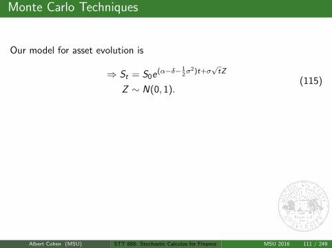
Monte Carlo Techniques
Our model for asset evolution is
⇒ St = S0e(α−δ− 12σ2)t+σ
√tZ
Z ∼ N(0, 1).(115)
Consider now the possibility of simulating the stock evolution bysimulating the random variable Z , or in fact an i.i.d. sequence
Z (i)
ni=1
.
For a European option with time expiry T , we can simulate the expirytime payoff mulitple times:
V(
S (i),T)
= G(
S (i))
= G(
S0e(α−δ− 12σ2)T+σ
√TZ (i)
). (116)
Albert Cohen (MSU) STT 888: Stochastic Calculus for Finance MSU 2016 111 / 249
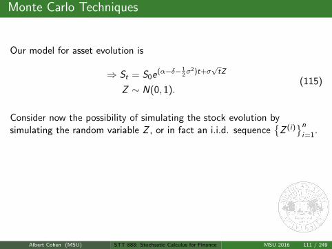
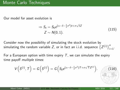
Monte Carlo Techniques
If we sample uniformly from our simulated values
V(
S (i),T)n
i=1we
can appeal to a sampling-convergence theorem with the appoximation
V (S , 0) = e−rT1
n
n∑i=1
V(
S (i),T). (117)
The challenge now is to simulate our lognormally distributed assetevolution.
One can simulate the value ST directly by one random variable Z , or amultiple of them to simulate the path of the evolution until T .
The latter method is necessary for Asian options.
Albert Cohen (MSU) STT 888: Stochastic Calculus for Finance MSU 2016 112 / 249
Monte Carlo Techniques
There are multiple ways to simulate Z . One way is to find a randomnumber U taken from a uniform distribution U[0, 1].
It follows that one can now map U → Z via inversion of the Nornal cdf N:
Z = N−1(U). (118)
It can be shown that in a sample, the standard deviation of the sampleaverage σsample is related to the standard deviation of an individual drawvia
σsample =σdraw√
n. (119)
If σdraw = σ, then we can see that we must increase our sample size by22k if we wish to cut our σsample by a factor of 2k .
Albert Cohen (MSU) STT 888: Stochastic Calculus for Finance MSU 2016 113 / 249
Brownian Motion
Consider a probability space (Ω,F ,P) and a process (Wt ,Ft) that lives onit, where Ft represents all the information about Wu0≤u≤t . Assumethat our pair satisfies, for s, t ≥ 0 and Aini=1 ⊆ F
P[W0 = 0] = 1
P[Wt ∈ dx ] = 1√2πt
e−x2
2t dx
P[limt→s Wt = Ws ] = 1
P[Wt+s −Ws ∈ A | Fs ] = P[Wt ∈ A] for all A ∈ FP[∩ni=1
Wti −Wti−1 ∈ Ai
] = Πn
i=1P[Wti −Wti−1 ∈ Ai ]
What’s so hard about that? Take a Z ∼ N(0, 1) and define
Xt =√
tZ (120)
Albert Cohen (MSU) STT 888: Stochastic Calculus for Finance MSU 2016 114 / 249
Quadratic Variation
Clearly, the last quantity, also known as independent increments, is whatmakes Brownian motion truly special. We can use this property to defineother, related properties. The first is the notion of quadratic variation.Simply put,
Wt+∆t −Wt ∼W∆t (121)
and so, for an i.i.d. N(0, 1) sequence Zini=1
n∑j=1
(Wtj+1 −Wtj
)2 ∼n∑
j=1
(Wtj+1−tj
)2
∼n∑
j=1
(√tj+1 − tjZj
)2
(122)
Albert Cohen (MSU) STT 888: Stochastic Calculus for Finance MSU 2016 115 / 249
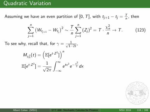
Quadratic Variation
Assuming we have an even partition of [0,T ], with tj+1 − tj = Tn , then
n∑j=1
(Wtj+1 −Wtj
)2 ∼ T
n
n∑j=1
(Zj)2 = T · χ
2n
n→ T . (123)
To see why, recall that, for γ = 1√1−2t
,
Mχ2n(t) =
(E[et·Z
2])n
E[et·Z2] =
1√2π
∫ ∞−∞
etx2e−
x2
2 dx
=1√2π
∫ ∞−∞
e− x2
2γ2 dx
=1√
1− 2t
⇒ Mχ2nn
(t) =1√
(1− 2 tn )n→ et = E[et·1].
(124)
Albert Cohen (MSU) STT 888: Stochastic Calculus for Finance MSU 2016 116 / 249
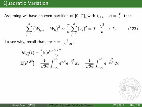
Quadratic Variation
Assuming we have an even partition of [0,T ], with tj+1 − tj = Tn , then
n∑j=1
(Wtj+1 −Wtj
)2 ∼ T
n
n∑j=1
(Zj)2 = T · χ
2n
n→ T . (123)
To see why, recall that, for γ = 1√1−2t
,
Mχ2n(t) =
(E[et·Z
2])n
E[et·Z2] =
1√2π
∫ ∞−∞
etx2e−
x2
2 dx =1√2π
∫ ∞−∞
e− x2
2γ2 dx
=1√
1− 2t
⇒ Mχ2nn
(t) =1√
(1− 2 tn )n→ et = E[et·1].
(124)
Albert Cohen (MSU) STT 888: Stochastic Calculus for Finance MSU 2016 116 / 249
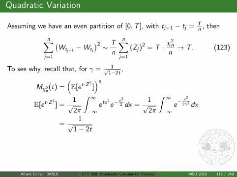
Quadratic Variation
Assuming we have an even partition of [0,T ], with tj+1 − tj = Tn , then
n∑j=1
(Wtj+1 −Wtj
)2 ∼ T
n
n∑j=1
(Zj)2 = T · χ
2n
n→ T . (123)
To see why, recall that, for γ = 1√1−2t
,
Mχ2n(t) =
(E[et·Z
2])n
E[et·Z2] =
1√2π
∫ ∞−∞
etx2e−
x2
2 dx =1√2π
∫ ∞−∞
e− x2
2γ2 dx
=1√
1− 2t
⇒ Mχ2nn
(t) =1√
(1− 2 tn )n→ et = E[et·1].
(124)
Albert Cohen (MSU) STT 888: Stochastic Calculus for Finance MSU 2016 116 / 249
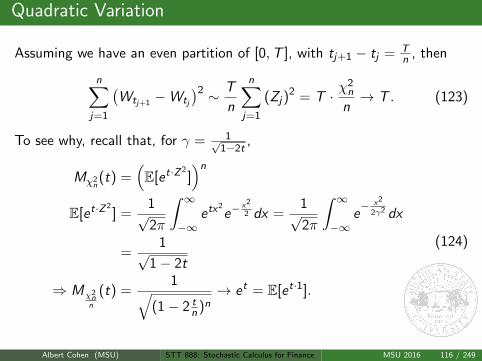
Quadratic Variation
Assuming we have an even partition of [0,T ], with tj+1 − tj = Tn , then
n∑j=1
(Wtj+1 −Wtj
)2 ∼ T
n
n∑j=1
(Zj)2 = T · χ
2n
n→ T . (123)
To see why, recall that, for γ = 1√1−2t
,
Mχ2n(t) =
(E[et·Z
2])n
E[et·Z2] =
1√2π
∫ ∞−∞
etx2e−
x2
2 dx =1√2π
∫ ∞−∞
e− x2
2γ2 dx
=1√
1− 2t
⇒ Mχ2nn
(t) =1√
(1− 2 tn )n→ et = E[et·1].
(124)
Albert Cohen (MSU) STT 888: Stochastic Calculus for Finance MSU 2016 116 / 249
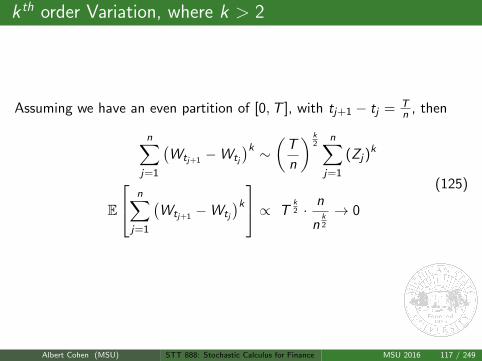
k th order Variation, where k > 2
Assuming we have an even partition of [0,T ], with tj+1 − tj = Tn , then
n∑j=1
(Wtj+1 −Wtj
)k ∼ (T
n
) k2
n∑j=1
(Zj)k
E
n∑j=1
(Wtj+1 −Wtj
)k ∝ Tk2 · n
nk2
→ 0
(125)
Albert Cohen (MSU) STT 888: Stochastic Calculus for Finance MSU 2016 117 / 249
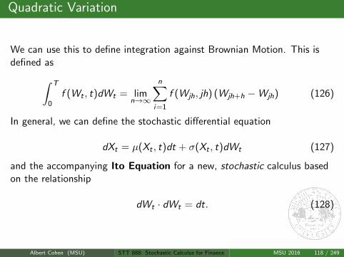
Quadratic Variation
We can use this to define integration against Brownian Motion. This isdefined as∫ T
0f (Wt , t)dWt = lim
n→∞
n∑i=1
f (Wjh, jh) (Wjh+h −Wjh) (126)
In general, we can define the stochastic differential equation
dXt = µ(Xt , t)dt + σ(Xt , t)dWt (127)
and the accompanying Ito Equation for a new, stochastic calculus basedon the relationship
dWt · dWt = dt. (128)
Albert Cohen (MSU) STT 888: Stochastic Calculus for Finance MSU 2016 118 / 249
Black-Scholes-Merton Analysis
Independent of the model for evolution of underlying asset, pricingmust be arbitrage-free
Achieve this via replication of derivative up to end of term of contract
Mathematical tools we require are now more involved than linearalgebra; namely Ito Calculus and Partial Differential Equations
To enable this analysis, assume the following for the model
∃ (Ω,F ,P) for which Wt is a standard Brownian motion.
dSt = St (µdt + σdWt), a Geometric Brownian Motion models theasset evolution
For a function f (x , t) ∈ C 2,1(R2 × R
)and Yt ≡ f (Wt , t), Ito
Calculus gives us:
dYt =(ft(Wt , t) + 1
2 fxx(Wt , t))
dt + fx(Wt , t)dWt
Albert Cohen (MSU) STT 888: Stochastic Calculus for Finance MSU 2016 119 / 249
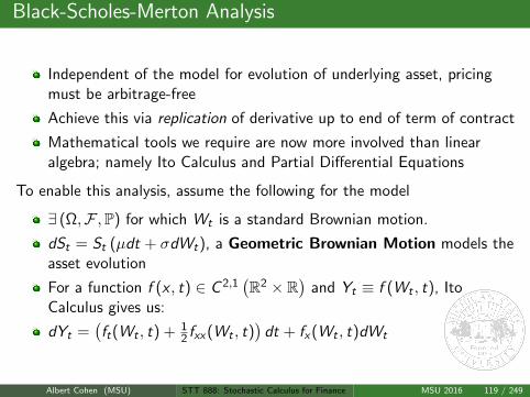
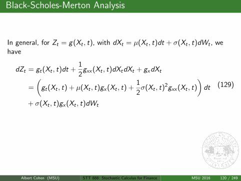
Black-Scholes-Merton Analysis
In general, for Zt = g(Xt , t), with dXt = µ(Xt , t)dt + σ(Xt , t)dWt , wehave
dZt = gt(Xt , t)dt +1
2gxx(Xt , t)dXtdXt + gxdXt
=
(gt(Xt , t) + µ(Xt , t)gx(Xt , t) +
1
2σ(Xt , t)2gxx(Xt , t)
)dt
+ σ(Xt , t)gx(Xt , t)dWt
(129)
Using the above assumptions, we arrive at the conclusion that we mustconstruct a portfolio Xt that matches the value Vt of the derivative wewish to price at all times t ≤ T , where T is the term of the contract.
Albert Cohen (MSU) STT 888: Stochastic Calculus for Finance MSU 2016 120 / 249
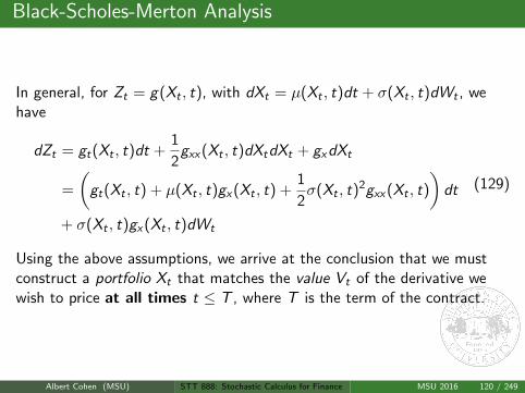
Black-Scholes-Merton Analysis
We match
dXt = dVt
XT = VT = G (ST )(130)
where G (S) is the payoff of the contract at time T if the value of theunderlying asset ST = S .
Albert Cohen (MSU) STT 888: Stochastic Calculus for Finance MSU 2016 121 / 249
Black-Scholes-Merton Analysis
We match
dXt = dVt
XT = VT = G (ST )(130)
where G (S) is the payoff of the contract at time T if the value of theunderlying asset ST = S .
Albert Cohen (MSU) STT 888: Stochastic Calculus for Finance MSU 2016 121 / 249
Black-Scholes-Merton Analysis
We match
dXt = dVt
XT = VT = G (ST )(130)
where G (S) is the payoff of the contract at time T if the value of theunderlying asset ST = S .
Albert Cohen (MSU) STT 888: Stochastic Calculus for Finance MSU 2016 121 / 249
Black-Scholes-Merton Analysis
To achieve this, we recognize that Xt = Vt ⇒ dXt = dVt and by theassumption V = V (St , t), Ito provides:
dXt = r (Xt −∆tSt) dt + ∆tdSt = r (Vt −∆tSt) dt + ∆tdSt
dVt =
(∂V
∂t(St , t) +
1
2σ2S2
t
∂2V
∂S2(St , t)
)dt +
∂V
∂S(St , t)dSt .
(131)
This is due to the fact that dSt = µStdt + σStdWt ⇒ (dSt)2 = σ2S2
t dt.
Albert Cohen (MSU) STT 888: Stochastic Calculus for Finance MSU 2016 122 / 249
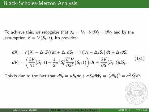
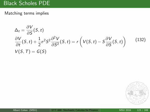
Black Scholes PDE
Matching terms implies
∆t =∂V
∂S(S , t)
∂V
∂t(S , t) +
1
2σ2S2∂
2V
∂S2(S , t) = r
(V (S , t)− S
∂V
∂S(S , t)
)V (S ,T ) = G (S)
(132)
This is the famous B-S-M PDE formulation for European option pricing,with payoff G (S). The question now - how do we solve it?!
Note:For dSt = µStdt + σStdWt , we have as the solution
St = Sue(µ− 12σ2)(t−u)+σ(Wt−Wu)
∼ Sue(µ− 12σ2)(t−u)+σWt−u
∼ Sue(µ− 12σ2)(t−u)+σ
√t−uZ .
(133)
Albert Cohen (MSU) STT 888: Stochastic Calculus for Finance MSU 2016 123 / 249
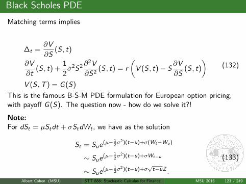
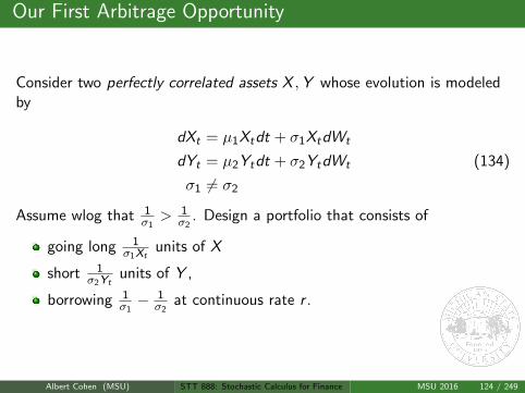
Our First Arbitrage Opportunity
Consider two perfectly correlated assets X ,Y whose evolution is modeledby
dXt = µ1Xtdt + σ1XtdWt
dYt = µ2Ytdt + σ2YtdWt
σ1 6= σ2
(134)
Assume wlog that 1σ1> 1
σ2. Design a portfolio that consists of
going long 1σ1Xt
units of X
short 1σ2Yt
units of Y ,
borrowing 1σ1− 1
σ2at continuous rate r .
Albert Cohen (MSU) STT 888: Stochastic Calculus for Finance MSU 2016 124 / 249
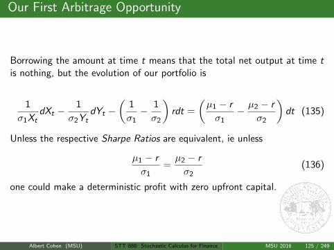
Our First Arbitrage Opportunity
Borrowing the amount at time t means that the total net output at time tis nothing, but the evolution of our portfolio is
1
σ1XtdXt −
1
σ2YtdYt −
(1
σ1− 1
σ2
)rdt =
(µ1 − r
σ1− µ2 − r
σ2
)dt (135)
Unless the respective Sharpe Ratios are equivalent, ie unless
µ1 − r
σ1=µ2 − r
σ2(136)
one could make a deterministic profit with zero upfront capital.
Albert Cohen (MSU) STT 888: Stochastic Calculus for Finance MSU 2016 125 / 249
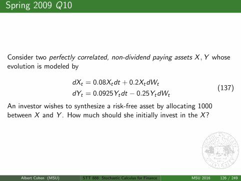
Spring 2009 Q10
Consider two perfectly correlated, non-dividend paying assets X ,Y whoseevolution is modeled by
dXt = 0.08Xtdt + 0.2XtdWt
dYt = 0.0925Ytdt − 0.25YtdWt(137)
An investor wishes to synthesize a risk-free asset by allocating 1000between X and Y . How much should she initially invest in the X ?
Albert Cohen (MSU) STT 888: Stochastic Calculus for Finance MSU 2016 126 / 249
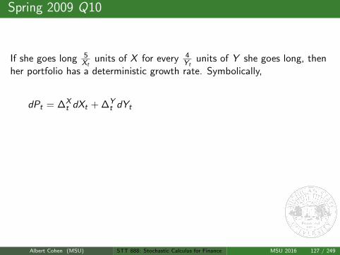
Spring 2009 Q10
If she goes long 5Xt
units of X for every 4Yt
units of Y she goes long, thenher portfolio has a deterministic growth rate. Symbolically,
dPt = ∆Xt dXt + ∆Y
t dYt
=5
Xt(0.08Xtdt + 0.2XtdWt) +
4
Yt(0.0925Ytdt − 0.25YtdWt)
= 0.77dt(138)
So, for every 9 units she spends initially, she has 5 invested in X . It followsthat if she spends 1000 initially, 5
9 · 1000 is invested in X to obtain a riskfree asset.
Albert Cohen (MSU) STT 888: Stochastic Calculus for Finance MSU 2016 127 / 249
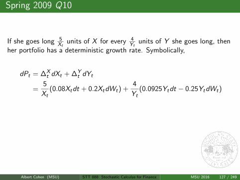
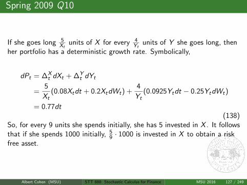
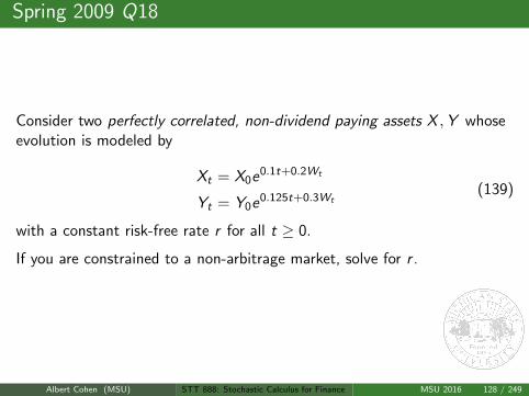
Spring 2009 Q18
Consider two perfectly correlated, non-dividend paying assets X ,Y whoseevolution is modeled by
Xt = X0e0.1t+0.2Wt
Yt = Y0e0.125t+0.3Wt(139)
with a constant risk-free rate r for all t ≥ 0.
If you are constrained to a non-arbitrage market, solve for r .
Albert Cohen (MSU) STT 888: Stochastic Calculus for Finance MSU 2016 128 / 249
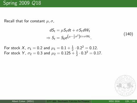
Spring 2009 Q18
Recall that for constant µ, σ,
dSt = µStdt + σStdWt
⇒ St = S0e(µ− 12σ2)t+σWt .
(140)
For stock X , σ1 = 0.2 and µ1 = 0.1 + 12 · 0.2
2 = 0.12.For stock Y , σ2 = 0.3 and µ2 = 0.125 + 1
2 · 0.32 = 0.17.
Since the two assets are perfectly correlated, their Sharpe ratios are equal:
µ1 − r
σ1=µ2 − r
σ2
⇒ r = 0.02.(141)
Albert Cohen (MSU) STT 888: Stochastic Calculus for Finance MSU 2016 129 / 249
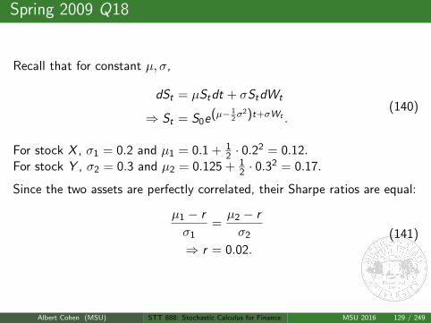
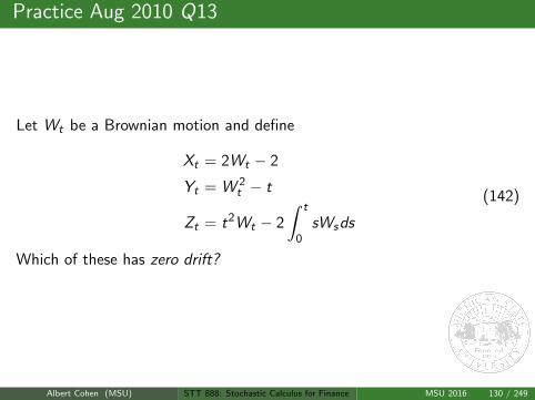
Practice Aug 2010 Q13
Let Wt be a Brownian motion and define
Xt = 2Wt − 2
Yt = W 2t − t
Zt = t2Wt − 2
∫ t
0sWsds
(142)
Which of these has zero drift?
Albert Cohen (MSU) STT 888: Stochastic Calculus for Finance MSU 2016 130 / 249
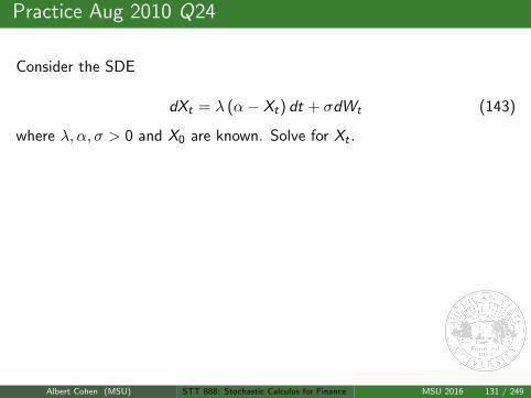
Practice Aug 2010 Q24
Consider the SDE
dXt = λ (α− Xt) dt + σdWt (143)
where λ, α, σ > 0 and X0 are known. Solve for Xt .
Answer:Using integrating factor eλt , we compute
d(
eλtXt
)= αλeλtdt + σeλtdWt
⇒ eλtXt − X0 = α(eλt − 1) + σ
∫ t
0eλsdWs
⇒ Xt = X0e−λt + α(1− e−λt) + σe−λt∫ t
0eλsdWs .
(144)
Bonus: Can we compute limt→∞ Xt in some meaningful way?
Albert Cohen (MSU) STT 888: Stochastic Calculus for Finance MSU 2016 131 / 249
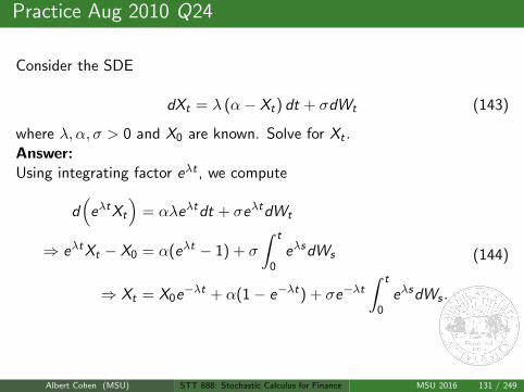
Practice Aug 2010 Q24
Consider the SDE
dXt = λ (α− Xt) dt + σdWt (143)
where λ, α, σ > 0 and X0 are known. Solve for Xt .Answer:Using integrating factor eλt , we compute
d(
eλtXt
)= αλeλtdt + σeλtdWt
⇒ eλtXt − X0 = α(eλt − 1) + σ
∫ t
0eλsdWs
⇒ Xt = X0e−λt + α(1− e−λt) + σe−λt∫ t
0eλsdWs .
(144)
Bonus: Can we compute limt→∞ Xt in some meaningful way?
Albert Cohen (MSU) STT 888: Stochastic Calculus for Finance MSU 2016 131 / 249
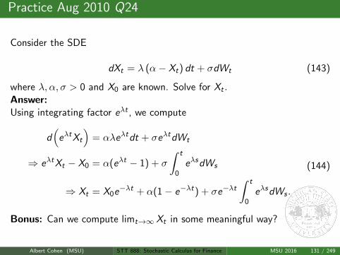
Practice Aug 2010 Q24
Consider the SDE
dXt = λ (α− Xt) dt + σdWt (143)
where λ, α, σ > 0 and X0 are known. Solve for Xt .Answer:Using integrating factor eλt , we compute
d(
eλtXt
)= αλeλtdt + σeλtdWt
⇒ eλtXt − X0 = α(eλt − 1) + σ
∫ t
0eλsdWs
⇒ Xt = X0e−λt + α(1− e−λt) + σe−λt∫ t
0eλsdWs .
(144)
Bonus: Can we compute limt→∞ Xt in some meaningful way?
Albert Cohen (MSU) STT 888: Stochastic Calculus for Finance MSU 2016 131 / 249
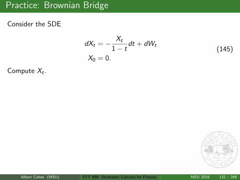
Practice: Brownian Bridge
Consider the SDE
dXt = − Xt
1− tdt + dWt
X0 = 0.(145)
Compute Xt .
Answer:Using integrating factor 1
1−t , we compute
d( Xt
1− t
)=
1
1− tdWt
⇒ Xt
1− t− X0 =
∫ t
0
1
1− sdWs
⇒ Xt = (1− t)
∫ t
0
1
1− sdWs .
(146)
Bonus: Can we compute limt→1 Xt in some meaningful way?
Albert Cohen (MSU) STT 888: Stochastic Calculus for Finance MSU 2016 132 / 249
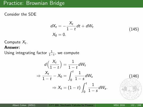
Practice: Brownian Bridge
Consider the SDE
dXt = − Xt
1− tdt + dWt
X0 = 0.(145)
Compute Xt .Answer:Using integrating factor 1
1−t , we compute
d( Xt
1− t
)=
1
1− tdWt
⇒ Xt
1− t− X0 =
∫ t
0
1
1− sdWs
⇒ Xt = (1− t)
∫ t
0
1
1− sdWs .
(146)
Bonus: Can we compute limt→1 Xt in some meaningful way?
Albert Cohen (MSU) STT 888: Stochastic Calculus for Finance MSU 2016 132 / 249
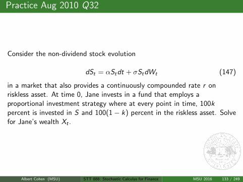
Practice Aug 2010 Q32
Consider the non-dividend stock evolution
dSt = αStdt + σStdWt (147)
in a market that also provides a continuously compounded rate r onriskless asset. At time 0, Jane invests in a fund that employs aproportional investment strategy where at every point in time, 100kpercent is invested in S and 100(1− k) percent in the riskless asset. Solvefor Jane’s wealth Xt .
Albert Cohen (MSU) STT 888: Stochastic Calculus for Finance MSU 2016 133 / 249
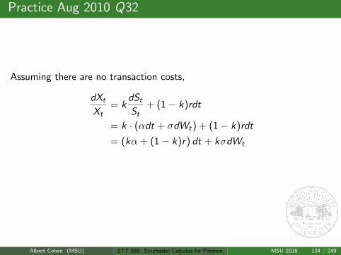
Practice Aug 2010 Q32
Assuming there are no transaction costs,
dXt
Xt= k
dSt
St+ (1− k)rdt
= k · (αdt + σdWt) + (1− k)rdt
= (kα + (1− k)r) dt + kσdWt
Xt = X0e(kα+(1−k)r− 12
(kσ)2)t+kσWt
(148)
Albert Cohen (MSU) STT 888: Stochastic Calculus for Finance MSU 2016 134 / 249
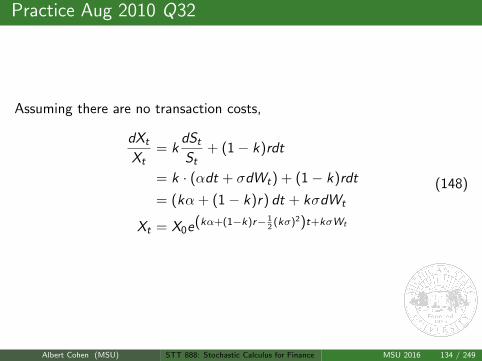
Practice Aug 2010 Q32
Assuming there are no transaction costs,
dXt
Xt= k
dSt
St+ (1− k)rdt
= k · (αdt + σdWt) + (1− k)rdt
= (kα + (1− k)r) dt + kσdWt
Xt = X0e(kα+(1−k)r− 12
(kσ)2)t+kσWt
(148)
Albert Cohen (MSU) STT 888: Stochastic Calculus for Finance MSU 2016 134 / 249
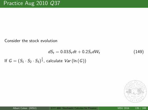
Practice Aug 2010 Q37
Consider the stock evolution
dSt = 0.03Stdt + 0.2StdWt (149)
If G = (S1 · S2 · S3)13 , calculate Var (ln (G ))
Albert Cohen (MSU) STT 888: Stochastic Calculus for Finance MSU 2016 135 / 249

Bonds, Forwards,Barriers
In any market, we have two basic assets that we use to price derivativeswith - a stock and a bond. Let’s see how these carry through to the BSMframework
If G (S) = 1 then at time T , one unit of bond (or currency) ispresented. What is the price at time 0?
If G (S) = Sa then at time T , one unit of stock (or asset) ispresented. What is the price at time 0?
If S0 = 50, and we agree to pay 1 unit of currency if the stock everhits 100, otherwise we pay nothing, what is the value of this financialinstrument at time 0?
By the BSM technology, we must find a solution to a PDE that satisfiesall conditions imposed by the definition of the contract we wish to price.For the first two cases above, there are only final time conditions.
Albert Cohen (MSU) STT 888: Stochastic Calculus for Finance MSU 2016 136 / 249
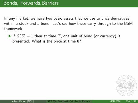
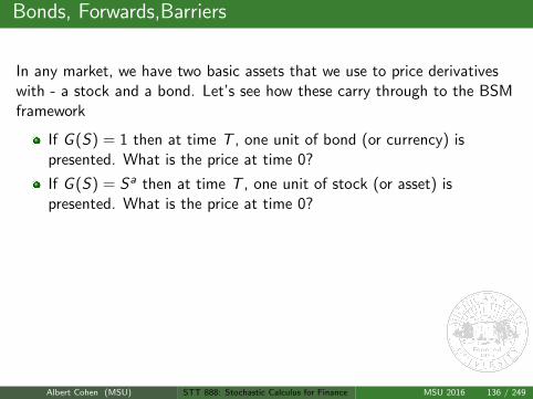
Bonds, Forwards,Barriers
For the case of presenting a unit of currency at time T , it is a fairassumption that the value V (S , t) should be independent of S , as thepayoff G (S) = 1 is.
Our resulting PDE is in fact an ODE for V (t):
V ′(t) = rV (t)
V (T ) = 1(150)
The solution of course is V (t) = e−r(T−t), which is the discountedvalue of one unit of currence T − t units of time in the future.
The hedging strategy is ∆ = ∂V∂S = 0, which means no stocks are held
to replicate this, and all the money taken at time t is invested inbuying e−r(T−t) units of bond.
Albert Cohen (MSU) STT 888: Stochastic Calculus for Finance MSU 2016 137 / 249
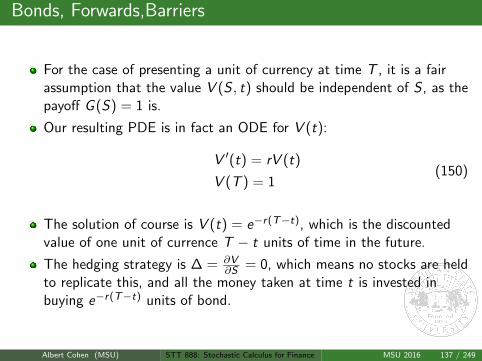
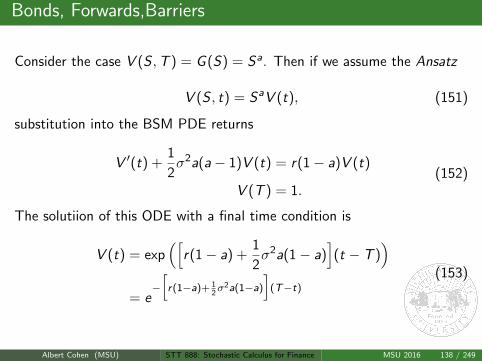
Bonds, Forwards,Barriers
Consider the case V (S ,T ) = G (S) = Sa. Then if we assume the Ansatz
V (S , t) = SaV (t), (151)
substitution into the BSM PDE returns
V ′(t) +1
2σ2a(a− 1)V (t) = r(1− a)V (t)
V (T ) = 1.(152)
The solutiion of this ODE with a final time condition is
V (t) = exp([
r(1− a) +1
2σ2a(1− a)
](t − T )
)= e
−[r(1−a)+ 1
2σ2a(1−a)
](T−t)
(153)
Albert Cohen (MSU) STT 888: Stochastic Calculus for Finance MSU 2016 138 / 249
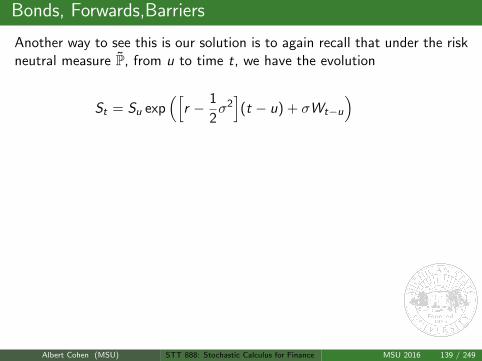
Bonds, Forwards,Barriers
Another way to see this is our solution is to again recall that under the riskneutral measure P, from u to time t, we have the evolution
St = Su exp([
r − 1
2σ2](t − u) + σWt−u
)
⇒ G (ST ) = SaT = Sa
t exp(
a[r − 1
2σ2](T − t) + aσWT−t
)⇒ V (S , t) = e−r(T−t)E[G (ST ) | St = S ]
= Sae−r(T−t)ea
[r− 1
2σ2
](T−t)
· E[eaσWT−t ]
= Sae−r(T−t)ea
[r− 1
2σ2
](T−t)
· e12a2σ2(T−t)
= Sae
[−r+ar− 1
2σ2a+ 1
2a2σ2
](T−t)
= Sae
[−r(1−a)− 1
2σ2a(1−a)
](T−t)
(154)
Albert Cohen (MSU) STT 888: Stochastic Calculus for Finance MSU 2016 139 / 249
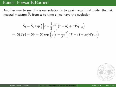
Bonds, Forwards,Barriers
Another way to see this is our solution is to again recall that under the riskneutral measure P, from u to time t, we have the evolution
St = Su exp([
r − 1
2σ2](t − u) + σWt−u
)⇒ G (ST ) = Sa
T = Sat exp
(a[r − 1
2σ2](T − t) + aσWT−t
)
⇒ V (S , t) = e−r(T−t)E[G (ST ) | St = S ]
= Sae−r(T−t)ea
[r− 1
2σ2
](T−t)
· E[eaσWT−t ]
= Sae−r(T−t)ea
[r− 1
2σ2
](T−t)
· e12a2σ2(T−t)
= Sae
[−r+ar− 1
2σ2a+ 1
2a2σ2
](T−t)
= Sae
[−r(1−a)− 1
2σ2a(1−a)
](T−t)
(154)
Albert Cohen (MSU) STT 888: Stochastic Calculus for Finance MSU 2016 139 / 249
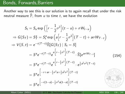
Bonds, Forwards,Barriers
Another way to see this is our solution is to again recall that under the riskneutral measure P, from u to time t, we have the evolution
St = Su exp([
r − 1
2σ2](t − u) + σWt−u
)⇒ G (ST ) = Sa
T = Sat exp
(a[r − 1
2σ2](T − t) + aσWT−t
)⇒ V (S , t) = e−r(T−t)E[G (ST ) | St = S ]
= Sae−r(T−t)ea
[r− 1
2σ2
](T−t)
· E[eaσWT−t ]
= Sae−r(T−t)ea
[r− 1
2σ2
](T−t)
· e12a2σ2(T−t)
= Sae
[−r+ar− 1
2σ2a+ 1
2a2σ2
](T−t)
= Sae
[−r(1−a)− 1
2σ2a(1−a)
](T−t)
(154)
Albert Cohen (MSU) STT 888: Stochastic Calculus for Finance MSU 2016 139 / 249

Bonds, Forwards,Barriers
In the last case, time is not explicitly given as a condition, meaning thatthe option is perpetual - only events to do with the the underlying stockvalue S will factor into the price of the contract. Hence, we have again asimpler ODE for V (S), but now with boundary conditions:
1
2σ2S2V ′′(S) = r
(V (S)− SV ′(S)
)V (0) = 0
V (100) = 1
(155)
General solution of this ODE is
V (S) = c1S + c2S−2rσ2 . (156)
Solution of this ODE with our boundary conditions leads to the closedform V (S) = 1
100 S , and so the specific price asked for is V (50) = 0.50
Albert Cohen (MSU) STT 888: Stochastic Calculus for Finance MSU 2016 140 / 249
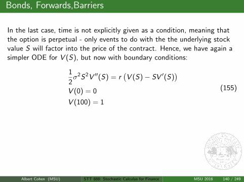
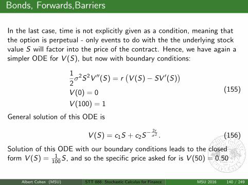
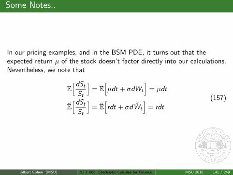
Some Notes..
In our pricing examples, and in the BSM PDE, it turns out that theexpected return µ of the stock doesn’t factor directly into our calculations.Nevertheless, we note that
E[dSt
St
]= E
[µdt + σdWt
]= µdt
E[dSt
St
]= E
[rdt + σdWt
]= rdt
(157)
Albert Cohen (MSU) STT 888: Stochastic Calculus for Finance MSU 2016 141 / 249
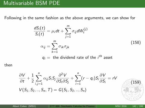
Multivariable BSM PDE
Following in the same fashion as the above arguments, we can show for
dSi (t)
Si (t)= µidt +
m∑j=1
σijdW(j)t
αij =m∑
k=1
σikσjk
qi = the dividend rate of the i th asset
(158)
then
∂V
∂t+
1
2
n∑i ,j=1
αijSiSj∂2V
∂Si∂Sj+
n∑i=1
(r − qi )Si∂V
∂Si= rV
V (S1,S2, ..,Sn,T ) = G (S1, S2, ..,Sn)
(159)
Albert Cohen (MSU) STT 888: Stochastic Calculus for Finance MSU 2016 142 / 249
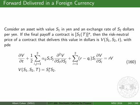
Forward Delivered in a Foreign Currency
Consider an asset with value S1 in yen and an exchange rate of S2 dollarsper yen. If the final payoff a contract is [S1(T )]a, then the risk-neutralprice of a contract that delivers this value in dollars is V (S1,S2, t), withpde
∂V
∂t+
1
2
2∑i ,j=1
αijSiSj∂2V
∂Si∂Sj+
2∑i=1
(r − qi )Si∂V
∂Si= rV
V (S1,S2,T ) = Sa1 S2.
(160)
Albert Cohen (MSU) STT 888: Stochastic Calculus for Finance MSU 2016 143 / 249
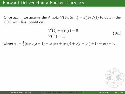
Forward Delivered in a Foreign Currency
Once again, we assume the Ansatz V (S1, S2, t) = Sa1 S2V (t) to obtain the
ODE with final condition:
V ′(t) + γV (t) = 0
V (T ) = 1,(161)
where γ := 12 (α11a(a− 1) + a(α12 + α21)) + a(r − q1) + (r − q2)− r .
It follows that
V (S1,S2, t) = Sa1 S2eγ(T−t). (162)
Note that for a = 1, our solution is
V (S1,S2, t) = S1S2er(T−t). (163)
Albert Cohen (MSU) STT 888: Stochastic Calculus for Finance MSU 2016 144 / 249
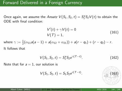

Options on Futures
It may be that it would be to an investor’s advantage to hold an optioncontract on an asset associated with the underlying (ie commodity, stock,etc...). One that is more liquid and involves lower transaction costsanyway than the one involving the actual asset.
One way to enable this liquidity is to write the contract on the associatedFuture or Forward contract. Recall that
F = Ser(T−t) (164)
and so
∂
∂S=
∂
∂F
∂F
∂S= er(T−t) ∂
∂F∂2
∂S2=
∂
∂S
(er(T−t) ∂
∂F
)= e2r(T−t) ∂
2
∂F 2
∂
∂t=
∂
∂t+
∂
∂F
∂F
∂t=
∂
∂t− rF
∂
∂F
(165)
Albert Cohen (MSU) STT 888: Stochastic Calculus for Finance MSU 2016 145 / 249
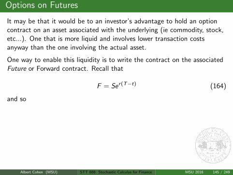
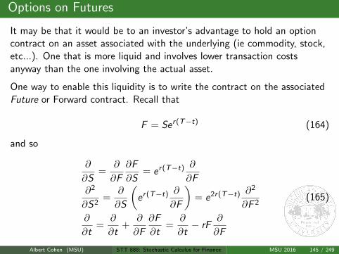
Options on Futures
The resulting B-S-M equation is
Vt +1
2σ2F 2VFF − rV = 0
V (F ,T ) = G (F )(166)
Question: How do we solve for V (F , t) ? Certainly, it is much closer toHeat equation than the original form of the B-S-M PDE.
Albert Cohen (MSU) STT 888: Stochastic Calculus for Finance MSU 2016 146 / 249
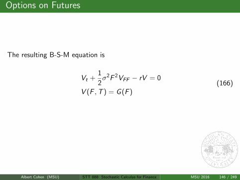
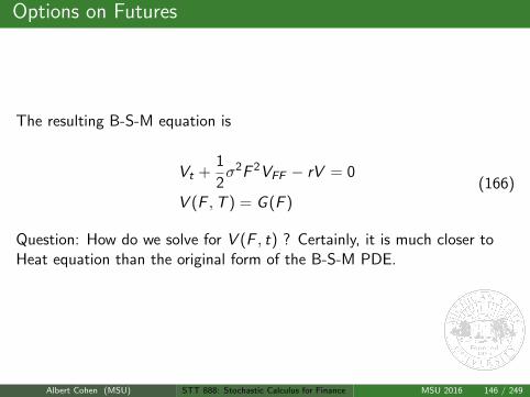
Path Dependent Options: Types and Technology
So far, we have mainly described the methodology for fairly pricing whatare known as Vanilla options,namely Puts, Calls and Forwards. These areonly time-dependent, in that the only event that the price is contingent onis the payoff at the end of the term, T .
A more exotic option would provide extra security by enabling thepurchaser to receive a payment contingent on an event related to theunderlying asset the option is written on. This event is most often the firsttime a stock price hits a certain theshold. However, the event could berelated to the average or running maximum of the stock price over a giventime window.
Albert Cohen (MSU) STT 888: Stochastic Calculus for Finance MSU 2016 147 / 249
Barrier Options
One of the initial examples of the B-S-M equation we were able to pricewas a perpetual barrier option. In that case, if a stock hit an upper barrierin its price, one dollar was paid to the option purchaser, otherwise theoption continues on.
In most cases, a time limit is put on such an option. What happens if wewish to put an extra barrier condition on an otherwise plain vanillaEuropean Call option?
Albert Cohen (MSU) STT 888: Stochastic Calculus for Finance MSU 2016 148 / 249

Recall: European Barrier Options
Consider now the case where an option is activated or deactivated,depending on whether or not the asset has reached a certain price level(barrier) before the option expires.
Hence, we have another path dependent option with the need for anothertracking variable. In this case, we can add the maximum or minimum ofthe asset over its path. They are knocked in or knocked out of action ifthe barrier is reached before expiry, depending on the contract design.
Albert Cohen (MSU) STT 888: Stochastic Calculus for Finance MSU 2016 149 / 249
Barrier Options: PDE Valuation
Consider a Down-and-Out Call Option:
∂V
∂t(S , t) +
1
2σ2S2∂
2V
∂S2(S , t) + r
(S∂V
∂S(S , t)− V (S , t)
)= 0
V (S ,T ) = (S − K )+
V (S , t) = 0 if S ≤ X
(167)
Albert Cohen (MSU) STT 888: Stochastic Calculus for Finance MSU 2016 150 / 249
Barrier Options
How do we solve such a PDE? Certainly, without this condition at X , wehave a solution of our plain Vanilla Call C (S , t). And, if X → 0, whatvalue should we should recover? Perhaps a modification of the solutionC (S , t) is a good place to start. With this in mind, we assume
V (S , t) = C (S , t)− B(S , t) (168)
where B(X , t) = C (X , t) and B(S , t) satisfies the same B-S-M PDE asthe European Call. This is reasonable assumption, as the B-S-M equationis linear.
Albert Cohen (MSU) STT 888: Stochastic Calculus for Finance MSU 2016 151 / 249
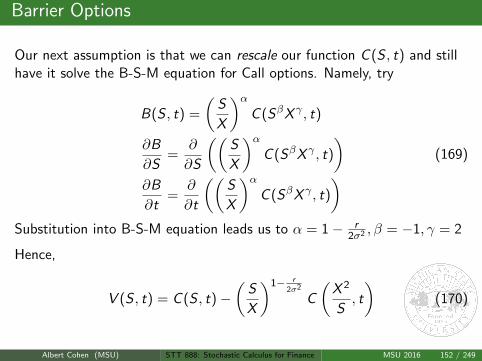
Barrier Options
Our next assumption is that we can rescale our function C (S , t) and stillhave it solve the B-S-M equation for Call options. Namely, try
B(S , t) =
(S
X
)αC (SβX γ , t)
∂B
∂S=
∂
∂S
((S
X
)αC (SβX γ , t)
)∂B
∂t=
∂
∂t
((S
X
)αC (SβX γ , t)
) (169)
Substitution into B-S-M equation leads us to α = 1− r2σ2 , β = −1, γ = 2
Hence,
V (S , t) = C (S , t)−(
S
X
)1− r2σ2
C
(X 2
S, t
)(170)
Albert Cohen (MSU) STT 888: Stochastic Calculus for Finance MSU 2016 152 / 249
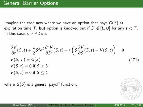
General Barrier Options
Imagine the case now where we have an option that pays G (S) atexpiration time T , but option is knocked out if St /∈ [L,U] for any t < T .In this case, our PDE is
∂V
∂t(S , t) +
1
2S2σ2∂
2V
∂S2(S , t) + r
(S∂V
∂S(S , t)− V (S , t)
)= 0
V (S ,T ) = G (S)
V (S , t) = 0 if S ≥ U
V (S , t) = 0 if S ≤ L
(171)
where G (S) is a general payoff function.
Albert Cohen (MSU) STT 888: Stochastic Calculus for Finance MSU 2016 153 / 249

Barrier Options
Once again, we can attempt a solution V (S , t) = A(t)B(S) and so weobtain:
A′(t)B(S) +1
2σ2A(t)S2B ′′(S) + r
(A(t)SB ′(S)− A(t)B(S)
)= 0
B(U) = 0
B(L) = 0
A(T )B(S) = G (S)
(172)
Modifications need to be made here if G (S) does not solve thecorresponding ODE for B(S).
Albert Cohen (MSU) STT 888: Stochastic Calculus for Finance MSU 2016 154 / 249
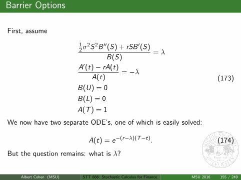
Barrier Options
First, assume
12σ
2S2B ′′(S) + rSB ′(S)
B(S)= λ
A′(t)− rA(t)
A(t)= −λ
B(U) = 0
B(L) = 0
A(T ) = 1
(173)
We now have two separate ODE’s, one of which is easily solved:
A(t) = e−(r−λ)(T−t). (174)
But the question remains: what is λ?
Albert Cohen (MSU) STT 888: Stochastic Calculus for Finance MSU 2016 155 / 249
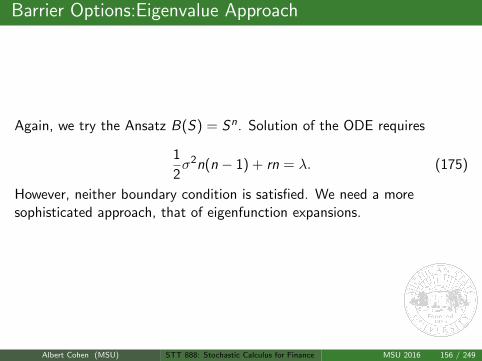
Barrier Options:Eigenvalue Approach
Again, we try the Ansatz B(S) = Sn. Solution of the ODE requires
1
2σ2n(n − 1) + rn = λ. (175)
However, neither boundary condition is satisfied. We need a moresophisticated approach, that of eigenfunction expansions.
Albert Cohen (MSU) STT 888: Stochastic Calculus for Finance MSU 2016 156 / 249
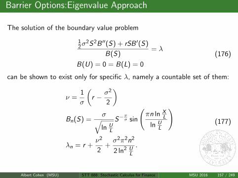
Barrier Options:Eigenvalue Approach
The solution of the boundary value problem
12σ
2S2B ′′(S) + rSB ′(S)
B(S)= λ
B(U) = 0 = B(L) = 0
(176)
can be shown to exist only for specific λ, namely a countable set of them:
ν =1
σ
(r − σ2
2
)Bn(S) =
σ√ln U
L
S−νσ sin
(πn ln X
L
ln UL
)
λn = r +ν2
2+σ2π2n2
2 ln2 UL
.
(177)
Albert Cohen (MSU) STT 888: Stochastic Calculus for Finance MSU 2016 157 / 249
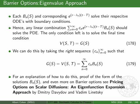
Barrier Options:Eigenvalue Approach
Each Bn(S) and corresponding e(r−λn)(t−T ) solve their respecitveODE’s with boundary conditions.
Hence, any linear combination∑∞
n=0 cne(r−λn)(t−T )Bn(S) shouldsolve the PDE. The only condition left is to solve the final timecondition
V (S ,T ) = G (S) (178)
We can do this by taking the right sequence cn∞n=0 such that
G (S) = V (S ,T ) =∞∑n=0
cnBn(S) (179)
For an explanation of how to do this, proof of the form of thesolutions Bn(S), and even more on Barrier options see PricingOptions on Scalar Diffusions: An Eigenfunction ExpansionApproach by Dmitry Davydov and Vadim Linetsky
Albert Cohen (MSU) STT 888: Stochastic Calculus for Finance MSU 2016 158 / 249
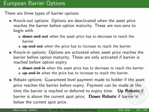
European Barrier Options
There are three types of barrier options:
Knock-out options: Options are deactivated when the asset pricereaches the barrier before option maturity. These are non-zero tobegin with.
down-and-out when the asset price has to decrease to reach thebarrier.up-and-out when the price has to increase to reach the barrier.
Knock-in options: Options are activated when asset price reaches thebarrier before option maturity. These are only activated if barrier isreached before option expiry.
down-and-in when the asset price has to decrease to reach the barrier.up-and-in when the price has to increase to reach the barrier.
Rebate options: Guaranteed level payment made to holder if the assetprice reaches the barrier before expiry. Payment can be made at thetime the barrier is reached or deferred to expiry time. Up Rebate ifbarrier is above the current spot price, Down Rebate if barrier isbelow the current spot price.
Albert Cohen (MSU) STT 888: Stochastic Calculus for Finance MSU 2016 159 / 249
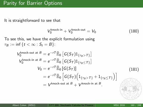
Parity for Barrier Options
It is straightforward to see that
V knock-in0 + V knock-out
0 = V0 (180)
To see this, we have the explicit formulation usingτB := inf t <∞ : St = B:
V knock-out at B0 = e−rT E0
[G (ST )1τB>T
]V knock-in at B
0 = e−rT E0
[G (ST )1τB≤T
]V0 = e−rT E0 [G (ST )]
= e−rT E0
[G (ST )
(1τB>T + 1τB≤T
)]= V knock-out at B + V knock-in at B .
(181)
Albert Cohen (MSU) STT 888: Stochastic Calculus for Finance MSU 2016 160 / 249
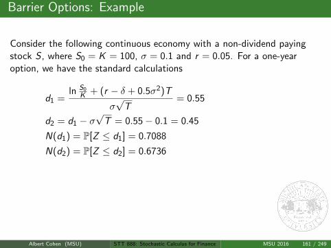
Barrier Options: Example
Consider the following continuous economy with a non-dividend payingstock S , where S0 = K = 100, σ = 0.1 and r = 0.05. For a one-yearoption, we have the standard calculations
d1 =ln S0
K + (r − δ + 0.5σ2)T
σ√
T= 0.55
d2 = d1 − σ√
T = 0.55− 0.1 = 0.45
N(d1) = P[Z ≤ d1] = 0.7088
N(d2) = P[Z ≤ d2] = 0.6736
⇒ V C0 = 100 · 0.7088− 100 · e−0.05 · 0.6736 = 6.805
⇒ V C ,knock-in at 990 = V C
0 = 6.805
⇒ V C ,knock-out at 990 = V C
0 − V C ,knock-in at 990 = 0.
(182)
Albert Cohen (MSU) STT 888: Stochastic Calculus for Finance MSU 2016 161 / 249
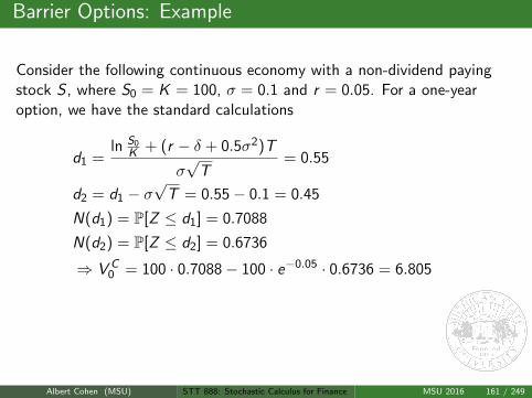
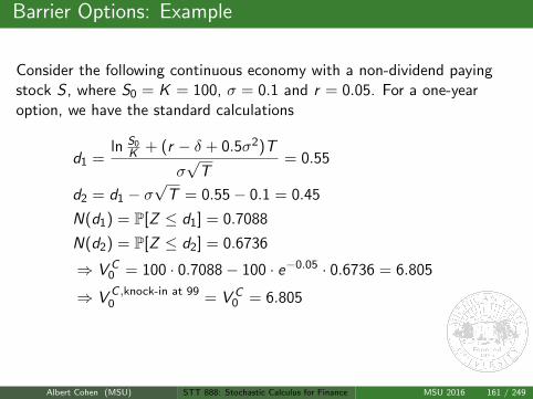
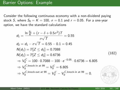
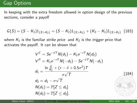
Gap Options
In keeping with the extra freedom allowed in option design of the previoussections, consider a payoff
G (S) = (S − K1)1S>K2 = (S − K2)1S>K2 + (K2 − K1)1S>K2 (183)
where K1 is the familiar strike price and K2 is the trigger price thatactivates the payoff. It can be shown that
V C = Se−δTN(d1)− K1e−rTN(d2)
V P = K1e−rTN(−d2)− Se−δTN(−d1)
d1 =ln S
K2+ (r − δ + 0.5σ2)T
σ√
T
d2 = d1 − σ√
T
N(d1) = P[Z ≤ d1]
N(d2) = P[Z ≤ d2].
(184)
Albert Cohen (MSU) STT 888: Stochastic Calculus for Finance MSU 2016 162 / 249
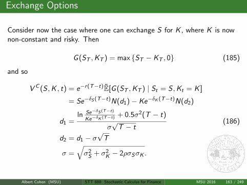
Exchange Options
Consider now the case where one can exchange S for K , where K is nownon-constant and risky. Then
G (ST ,KT ) = max ST − KT , 0 (185)
and so
V C (S ,K , t) = e−r(T−t)E[G (ST ,KT ) | St = S ,Kt = K ]
= Se−δS (T−t)N(d1)− Ke−δK (T−t)N(d2)
d1 =ln Se−δS (T−t)
Ke−δK (T−t) + 0.5σ2(T − t)
σ√
T − t
d2 = d1 − σ√
T
σ =√σ2S + σ2
K − 2ρσSσK .
(186)
Albert Cohen (MSU) STT 888: Stochastic Calculus for Finance MSU 2016 163 / 249
Asian Options:Options on Averages
Another useful example of a path dependent option that is commonlyemployed is the Asian option. As an example, an airline may only buy afinite supply of jet fuel every year, but use it continuously during the year.To guard itself against large price movements, the company may choose touse financial instruments with a fixed purchase date to avoid having tocontinuously hedge against the commodity price movements. We assumethat the asset evolves according to
dSt = µ(St , t)dt + σ(St , t)dWt (187)
on some fixed probability space (Ω,F ,P)
Albert Cohen (MSU) STT 888: Stochastic Calculus for Finance MSU 2016 164 / 249
Asian Options:Options on Averages
A common instrument used is a forward contract. However, this fixes theprice once the contract is signed. Another choice companies have is topurchase an Asian option that pays, at time T ,
max
(S − 1
T
∫ T
0Sudu, 0
)(188)
To be able to price this option at time t, two pieces of information arerequired:
St − the stock price
It :=
∫ t
0Sudu − the running integral of the stock price
(189)
Albert Cohen (MSU) STT 888: Stochastic Calculus for Finance MSU 2016 165 / 249
Asian Options:Options on Averages
Furthermore, we also require the differential form dIt :
dIt = Stdt. (190)
Albert Cohen (MSU) STT 888: Stochastic Calculus for Finance MSU 2016 166 / 249
Asian Options:Options on Averages
Furthermore, we also require the differential form dIt :
dIt = Stdt. (190)
Albert Cohen (MSU) STT 888: Stochastic Calculus for Finance MSU 2016 166 / 249
Asian Options:Options on Averages
With the triple of information (St , It , t), we can again construct aB-S-M portfolio replication argument.
On the one hand, we have the self-financing portfolio we construct,Xt using the underlying asset St and the riskless bank account:
dXt = r (Xt −∆St) dt + ∆tdSt . (191)
Albert Cohen (MSU) STT 888: Stochastic Calculus for Finance MSU 2016 167 / 249
Asian Options:Options on Averages
And on the other hand, we have the price of the contract Vt ≡ V (St , It , t)that satisfies Ito’s equation
dVt =
(∂V
∂t+
1
2σ(St , t)2∂
2V
∂S2
)dt +
∂V
∂SdSt +
∂V
∂IdIt
=
(∂V
∂t+
1
2σ(St , t)2∂
2V
∂S2+ St
∂V
∂I
)dt +
∂V
∂SdSt .
(192)
Albert Cohen (MSU) STT 888: Stochastic Calculus for Finance MSU 2016 168 / 249
Asian Options:Options on Averages
Matching terms once again, with the constraint that Vt = Xt , we obtain
∂V
∂t+
1
2σ(S , t)2∂
2V
∂S2+ S
∂V
∂I+ r
(S∂V
∂S− V
)= 0
V (S , I ,T ) = max
(S − I
T, 0
)∆ =
∂V
∂S
(193)
Albert Cohen (MSU) STT 888: Stochastic Calculus for Finance MSU 2016 169 / 249
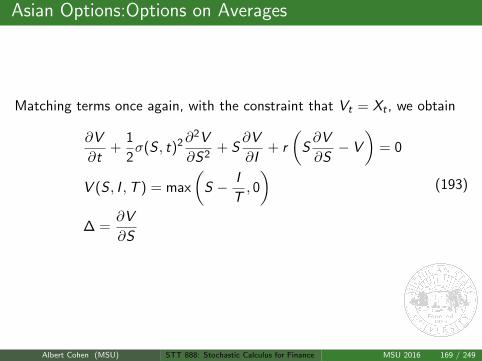
Asian Options:Options on Averages
Matching terms once again, with the constraint that Vt = Xt , we obtain
∂V
∂t+
1
2σ(S , t)2∂
2V
∂S2+ S
∂V
∂I+ r
(S∂V
∂S− V
)= 0
V (S , I ,T ) = max
(S − I
T, 0
)∆ =
∂V
∂S
(193)
Albert Cohen (MSU) STT 888: Stochastic Calculus for Finance MSU 2016 169 / 249
Asian Options:Similarity Solutions
This Asian option acts as a Call option contract, in that the strike Kis replaced by an average value over the path of the asset evolution.
But, the dimension of the PDE has increased by 1. This makes thesolution more difficult to obtain.
Still, we have the tools used in the solution of the heat equation andBarrier options, namely Similarity solutions.
We assume that
V (S , I , t) = S · H(R, t)
R ≡ I
S
V (S , I ,T ) = max
(S − I
T, 0
)= S ·max
(1− I
ST, 0
)= S ·max
(1− R
T, 0
)= S · H(R,T )
(194)
Albert Cohen (MSU) STT 888: Stochastic Calculus for Finance MSU 2016 170 / 249
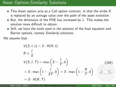
Asian Options:Similarity Solutions
Substitution into the B-S-M equation derived above returns
∂H
∂t+
1
2σ2R2∂
2H
∂R2+ (1− rR)
∂H
∂R= 0
H(R,T ) = max
(1− R
T, 0
) (195)
Albert Cohen (MSU) STT 888: Stochastic Calculus for Finance MSU 2016 171 / 249
Asian Options:Similarity Solutions
Substitution into the B-S-M equation derived above returns
∂H
∂t+
1
2σ2R2∂
2H
∂R2+ (1− rR)
∂H
∂R= 0
H(R,T ) = max
(1− R
T, 0
) (195)
Albert Cohen (MSU) STT 888: Stochastic Calculus for Finance MSU 2016 171 / 249
Asian Options:Similarity Solutions
For boundary conditions similar to those imposed on the European call, wesee that if R →∞, then it must be that S → 0, and so the value of theoption should be worthless:
H(∞, t) = 0 (196)
If R → 0, then assuming that all derivatives of H with respect to R arefinite, it is reasonable to return to the BSM equation to obtain
∂H
∂t(0, t) +
∂H
∂R(0, t) = 0 (197)
Use tools similiar to those used in explicit solution of original EuropeanCall option C (S , t) to solve this PDE.
Albert Cohen (MSU) STT 888: Stochastic Calculus for Finance MSU 2016 172 / 249
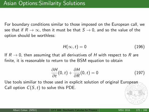
Lookback Options
Another exotic, path-dependent option that is studied is the Lookbackoption. This contract agrees to pay the investor the value
max (JT − ST , 0) (198)
where Jt ≡ max0≤u≤tSu
Such an option is valuable, as it helps to reduce the regret of an investorwho wishes to sell his asset S at its highest value over a window of time[0,T ].
Of course, only the actual asset S is traded in, not its maximum Jt at timet. It follows that our replicating portfolio Xt is constructed using S andthe bank account only.
Albert Cohen (MSU) STT 888: Stochastic Calculus for Finance MSU 2016 173 / 249
Lookback Options
Once again, our B-S-M replication argument returns
dXt = r (Xt −∆tSt) dt + ∆tdSt = r (Vt −∆tSt) dt + ∆tdSt
dVt =
(∂V
∂t+
1
2σ(St , t)2∂
2V
∂S2
)dt
+∂V
∂SdSt +
∂V
∂JdJt
=
(∂V
∂t+
1
2σ(St , t)2∂
2V
∂S2
)dt +
∂V
∂SdSt +
∂V
∂J1St=JtdSt
(199)
Albert Cohen (MSU) STT 888: Stochastic Calculus for Finance MSU 2016 174 / 249
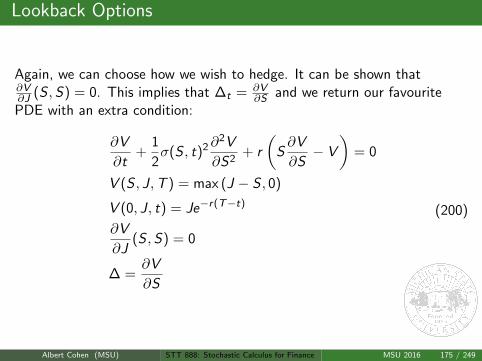
Lookback Options
Again, we can choose how we wish to hedge. It can be shown that∂V∂J (S ,S) = 0. This implies that ∆t = ∂V
∂S and we return our favouritePDE with an extra condition:
∂V
∂t+
1
2σ(S , t)2∂
2V
∂S2+ r
(S∂V
∂S− V
)= 0
V (S , J,T ) = max (J − S , 0)
V (0, J, t) = Je−r(T−t)
∂V
∂J(S ,S) = 0
∆ =∂V
∂S
(200)
Albert Cohen (MSU) STT 888: Stochastic Calculus for Finance MSU 2016 175 / 249
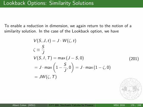
Lookback Options: Similarity Solutions
To enable a reduction in dimension, we again return to the notion of asimilarity solution. In the case of the Lookback option, we have
V (S , J, t) = J ·W (ζ, t)
ζ ≡ S
JV (S , I ,T ) = max (J − S , 0)
= J ·max
(1− S
J, 0
)= J ·max (1− ζ, 0)
= JW (ζ,T )
(201)
Albert Cohen (MSU) STT 888: Stochastic Calculus for Finance MSU 2016 176 / 249
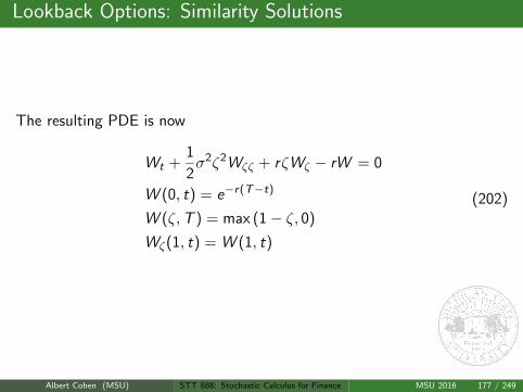
Lookback Options: Similarity Solutions
The resulting PDE is now
Wt +1
2σ2ζ2Wζζ + rζWζ − rW = 0
W (0, t) = e−r(T−t)
W (ζ,T ) = max (1− ζ, 0)
Wζ(1, t) = W (1, t)
(202)
Albert Cohen (MSU) STT 888: Stochastic Calculus for Finance MSU 2016 177 / 249
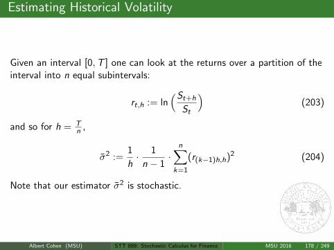
Estimating Historical Volatility
Given an interval [0,T ] one can look at the returns over a partition of theinterval into n equal subintervals:
rt,h := ln(St+h
St
)(203)
and so for h = Tn ,
σ2 :=1
h· 1
n − 1·
n∑k=1
(r(k−1)h,h)2 (204)
Note that our estimator σ2 is stochastic.
Albert Cohen (MSU) STT 888: Stochastic Calculus for Finance MSU 2016 178 / 249
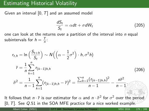
Estimating Historical Volatility
Given an interval [0,T ] and an assumed model
dSt
St= αdt + σdWt (205)
one can look at the returns over a partition of the interval into n equalsubintervals for h = T
n :
rt,h = ln(St+h
St
)∼ N
((α− 1
2σ2)· h, σ2h)
r =1
n
n∑k=1
r(k−1)h,h
σ2 =1
n − 1
n∑k=1
(r(k−1)h,h − r)2 =
∑nk=1(r(k−1)h,h)2
n − 1− nr 2
n − 1.
(206)
It follows that n · r is our estimator for α and n · σ2 for σ2 over the period[0,T ]. See Q.51 in the SOA MFE practice for a nice worked example.
Albert Cohen (MSU) STT 888: Stochastic Calculus for Finance MSU 2016 179 / 249
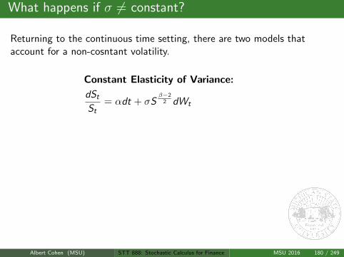
What happens if σ 6= constant?
Returning to the continuous time setting, there are two models thataccount for a non-cosntant volatility.
Constant Elasticity of Variance:
dSt
St= αdt + σS
β−22 dWt
Heston Model (Stochastic Volatility):
dSt
St= αdt +
√σtdWt
dσt = k · (σ(t)− σt)dt + σHdWt
dWt · dWt = ρdt.
(207)
Both lead to more mathematically complex solution techniques. However,empirical data suggests that they calibrate significantly better withobserved option data.
Albert Cohen (MSU) STT 888: Stochastic Calculus for Finance MSU 2016 180 / 249
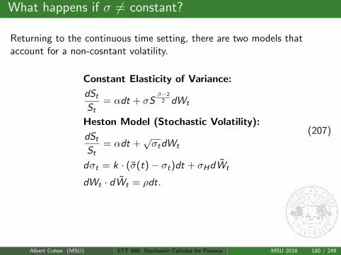
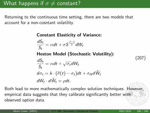
Interest Rate Derivatives
Consider a zero-coupon, non-defaultable bond that pays V (T ,T ) = 1 atexpiry date T . The risk-free rate is a function of time r(t).
The corresponding boundary value problem is (holding T fixed)
dV
V= r(t)dt
V (T ,T ) = 1.(208)
The solution is
V (t,T ) = e−∫ Tt r(s)ds . (209)
Albert Cohen (MSU) STT 888: Stochastic Calculus for Finance MSU 2016 181 / 249
Interest Rate Derivatives
Consider again a zero-coupon, non-defaultable bond that paysV (T ,T ) = 1 at expiry date T .
Now, the risk-free rate is a random variable indexed by time rt(ω) on a
probability space(
Ω,F ,P)
It follows that, if we have a related risk neutral measure P, then for astochastic process rt(ω), we expect the (martingale) solution
V (t,T ) = E[e−
∫ Tt rs(ω)ds
]. (210)
Albert Cohen (MSU) STT 888: Stochastic Calculus for Finance MSU 2016 182 / 249
Short Rate Model
For the evolution of interest rates r on(
Ω,F ,P)
, we can assume the
general model
drt = µ(rt , t)dt + σ(rt , t)dWt
dVt
Vt= α(rt , t)dt + σV (rt , t)dWt
(211)
Albert Cohen (MSU) STT 888: Stochastic Calculus for Finance MSU 2016 183 / 249
Short Rate Model
Consider now two bonds, one with expiry date T1 and the other withexpiry date T2. By the pricing formula
V (t,T1) = E[e−
∫ T1t rs(ω)ds
]V (t,T2) = E
[e−
∫ T2t rs(ω)ds
] (212)
where both are driven by the same Brownian motion W . It follows that,∀t, the Sharpe Ratios for bonds must be equal for any expiry date:
α(r , t)− r
σV (r , t)= λ(r , t) = Market Price of Risk . (213)
Albert Cohen (MSU) STT 888: Stochastic Calculus for Finance MSU 2016 184 / 249
Market Price of Risk
Recall from our initial discussion of equity models that under constant(µ, σ, r), the rate of return on a share of equity is
dSt
St= µdt + σdWt
= rdt + σdWt .
⇒ dWt = dWt +µ− r
σdt
= dWt + λdt
(214)
In words, the market price of risk, or Sharpe ratio, is the drift correctionthat allows us to transition from a Brownian motion under the physicalmeasure P to a Brownian motion under the risk-neutral measure P.
Albert Cohen (MSU) STT 888: Stochastic Calculus for Finance MSU 2016 185 / 249
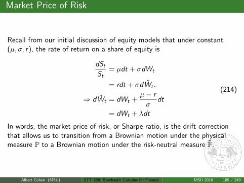
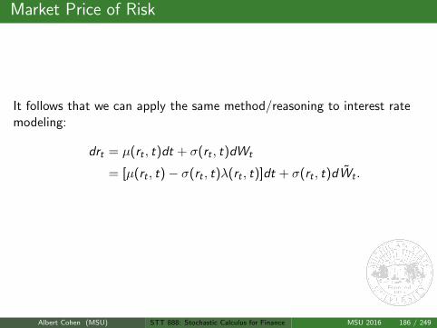
Market Price of Risk
It follows that we can apply the same method/reasoning to interest ratemodeling:
drt = µ(rt , t)dt + σ(rt , t)dWt
= [µ(rt , t)− σ(rt , t)λ(rt , t)]dt + σ(rt , t)dWt .
dWt = dWt + λ(rt , t)dt.
(215)
Albert Cohen (MSU) STT 888: Stochastic Calculus for Finance MSU 2016 186 / 249
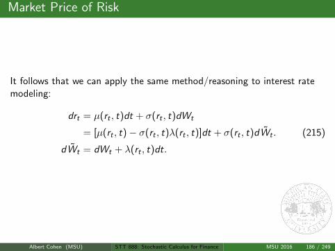
Market Price of Risk
It follows that we can apply the same method/reasoning to interest ratemodeling:
drt = µ(rt , t)dt + σ(rt , t)dWt
= [µ(rt , t)− σ(rt , t)λ(rt , t)]dt + σ(rt , t)dWt .
dWt = dWt + λ(rt , t)dt.
(215)
Albert Cohen (MSU) STT 888: Stochastic Calculus for Finance MSU 2016 186 / 249
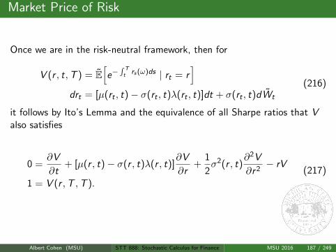
Market Price of Risk
Once we are in the risk-neutral framework, then for
V (r , t,T ) = E[e−
∫ Tt rs(ω)ds | rt = r
]drt = [µ(rt , t)− σ(rt , t)λ(rt , t)]dt + σ(rt , t)dWt
(216)
it follows by Ito’s Lemma and the equivalence of all Sharpe ratios that Valso satisfies
0 =∂V
∂t+ [µ(r , t)− σ(r , t)λ(r , t)]
∂V
∂r+
1
2σ2(r , t)
∂2V
∂r 2− rV
1 = V (r ,T ,T ).
(217)
Question: How do we determine the market price of risk λ?
Albert Cohen (MSU) STT 888: Stochastic Calculus for Finance MSU 2016 187 / 249
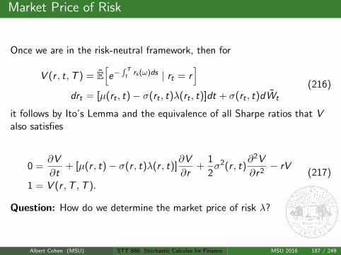
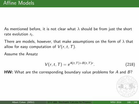
Affine Models
As mentioned before, it is not clear what λ should be from just the shortrate evolution rt .
There are models, however, that make assumptions on the form of λ thatallow for easy computation of V (r , t,T ).
Assume the Ansatz
V (r , t,T ) = eA(t,T )+B(t,T )r . (218)
HW: What are the corresponding boundary value problems for A and B?
Albert Cohen (MSU) STT 888: Stochastic Calculus for Finance MSU 2016 188 / 249
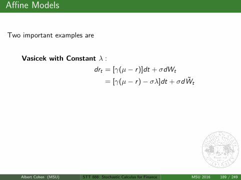
Affine Models
Two important examples are
Vasicek with Constant λ :
drt = [γ(µ− r)]dt + σdWt
= [γ(µ− r)− σλ]dt + σdWt
CIR with λ(r , t) =λ√
r
σ:
drt = [γ(µ− r)]dt + σ√
rtdWt
= [γ(µ− r)− λr ]dt + σ√
rtdWt .
(219)
HW: Solve the corresponding boundary value problems for A and B forboth the Vasicek and CIR models.
Albert Cohen (MSU) STT 888: Stochastic Calculus for Finance MSU 2016 189 / 249
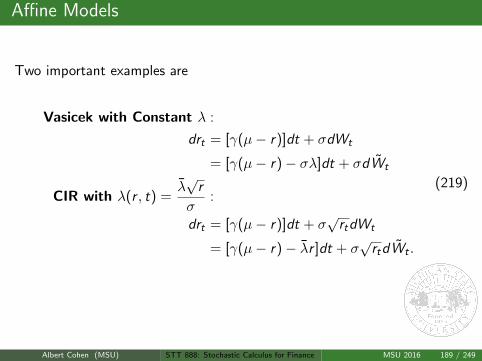
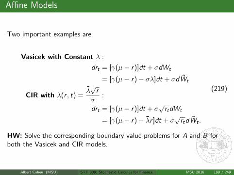
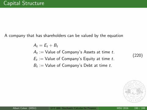
Capital Structure
A company that has shareholders can be valued by the equation
At = Et + Bt
At := Value of Company’s Assets at time t.
Et := Value of Company’s Equity at time t.
Bt := Value of Company’s Debt at time t.
(220)
Albert Cohen (MSU) STT 888: Stochastic Calculus for Finance MSU 2016 190 / 249
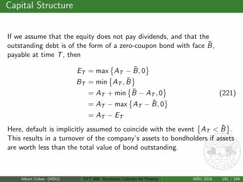
Capital Structure
If we assume that the equity does not pay dividends, and that theoutstanding debt is of the form of a zero-coupon bond with face B,payable at time T , then
ET = max
AT − B, 0
BT = min
AT , B
= AT + min
B − AT , 0
= AT −max
AT − B, 0
= AT − ET
(221)
Here, default is implicitly assumed to coincide with the event
AT < B
.This results in a turnover of the company’s assets to bondholders if assetsare worth less than the total value of bond outstanding.
Albert Cohen (MSU) STT 888: Stochastic Calculus for Finance MSU 2016 191 / 249
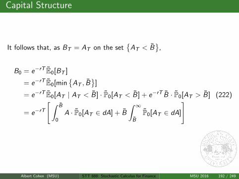
Capital Structure
It follows that, as BT = AT on the set
AT < B
,
B0 = e−rT E0[BT ]
= e−rT E0[min
AT , B
]
= e−rT E0[AT | AT < B] · P0[AT < B] + e−rT B · P0[AT > B]
= e−rT
[∫ B
0A · P0[AT ∈ dA] + B
∫ ∞B
P0[AT ∈ dA]
] (222)
Albert Cohen (MSU) STT 888: Stochastic Calculus for Finance MSU 2016 192 / 249
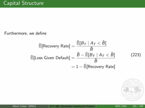
Capital Structure
Furthermore, we define
E[Recovery Rate] =E[BT | AT < B]
B
E[Loss Given Default] =B − E[BT | AT < B]
B
= 1− E[Recovery Rate]
(223)
Albert Cohen (MSU) STT 888: Stochastic Calculus for Finance MSU 2016 193 / 249
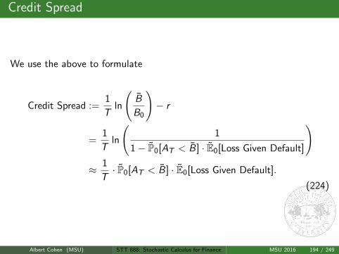
Credit Spread
We use the above to formulate
Credit Spread :=1
Tln
(B
B0
)− r
=1
Tln
(1
1− P0[AT < B] · E0[Loss Given Default]
)≈ 1
T· P0[AT < B] · E0[Loss Given Default].
(224)
Albert Cohen (MSU) STT 888: Stochastic Calculus for Finance MSU 2016 194 / 249
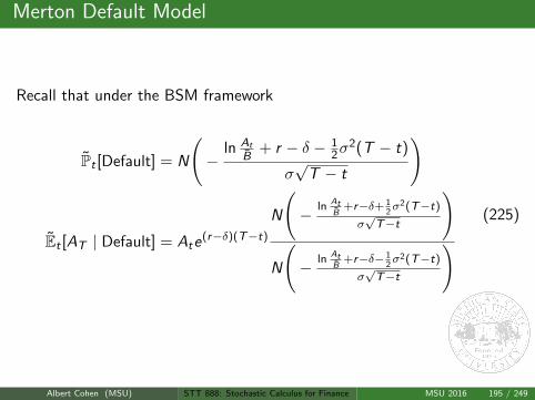
Merton Default Model
Recall that under the BSM framework
Pt [Default] = N
(−
ln At
B+ r − δ − 1
2σ2(T − t)
σ√
T − t
)
Et [AT | Default] = Ate(r−δ)(T−t)
N
(− ln At
B+r−δ+ 1
2σ2(T−t)
σ√T−t
)
N
(− ln At
B+r−δ− 1
2σ2(T−t)
σ√T−t
) (225)
Albert Cohen (MSU) STT 888: Stochastic Calculus for Finance MSU 2016 195 / 249
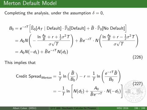
Merton Default Model
Completing the analysis, under the assumption δ = 0,
B0 = e−rT[E0[AT | Default] · P0[Default] + B · P0[No Default]
]= A0N
(−
ln A0
B+ r + 1
2σ2T
σ√
T
)+ Be−rT · N
(ln A0
B+ r − 1
2σ2T
σ√
T
)= A0N(−d1) + Be−rTN(d2)
(226)This implies that
Credit SpreadMerton =1
Tln( B
B0
)− r =
1
Tln
(e−rT B
B0
)
= − 1
Tln
[N(d2) +
A0
Be−rT· N(−d1)
] (227)
Q: What happens to the credit spread as T → 0 ?
Albert Cohen (MSU) STT 888: Stochastic Calculus for Finance MSU 2016 196 / 249
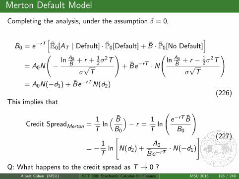
Merton Default Model
Completing the analysis, under the assumption δ = 0,
B0 = e−rT[E0[AT | Default] · P0[Default] + B · P0[No Default]
]= A0N
(−
ln A0
B+ r + 1
2σ2T
σ√
T
)+ Be−rT · N
(ln A0
B+ r − 1
2σ2T
σ√
T
)= A0N(−d1) + Be−rTN(d2)
(226)This implies that
Credit SpreadMerton =1
Tln( B
B0
)− r =
1
Tln
(e−rT B
B0
)
= − 1
Tln
[N(d2) +
A0
Be−rT· N(−d1)
] (227)
Q: What happens to the credit spread as T → 0 ?Albert Cohen (MSU) STT 888: Stochastic Calculus for Finance MSU 2016 196 / 249
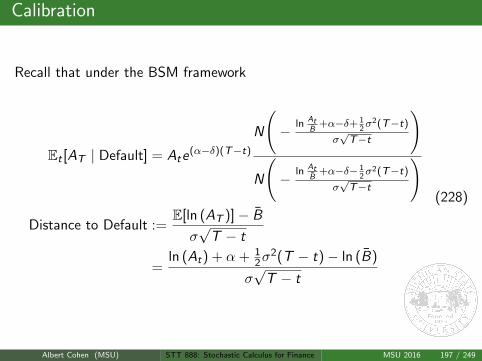
Calibration
Recall that under the BSM framework
Et [AT | Default] = Ate(α−δ)(T−t)
N
(− ln At
B+α−δ+ 1
2σ2(T−t)
σ√T−t
)
N
(− ln At
B+α−δ− 1
2σ2(T−t)
σ√T−t
)
Distance to Default :=E[ln (AT )]− B
σ√
T − t
=ln (At) + α + 1
2σ2(T − t)− ln (B)
σ√
T − t
(228)
Albert Cohen (MSU) STT 888: Stochastic Calculus for Finance MSU 2016 197 / 249
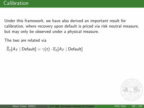
Calibration
Under this framework, we have also derived an important result forcalibration, where recovery upon default is priced via risk neutral measure,but may only be observed under a physical measure.
The two are related via
Et [AT | Default] = γ(t) · Et [AT | Default]
γ := e(r−α)(T−t)
N
(− ln At
B+r−δ+ 1
2σ2(T−t)
σ√T−t
)
N
(− ln At
B+r−δ− 1
2σ2(T−t)
σ√T−t
) N
(− ln At
B+α−δ− 1
2σ2(T−t)
σ√T−t
)
N
(− ln At
B+α−δ+ 1
2σ2(T−t)
σ√T−t
)(229)
Note that γ(t) = 1 for all 0 ≤ t ≤ T if α = r .
Albert Cohen (MSU) STT 888: Stochastic Calculus for Finance MSU 2016 198 / 249
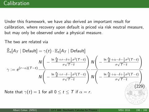

Solving the BSM PDE:
Lemma
Under a change of variables, solving the BSM PDE is equivalent to solvingthe Heat Equation
uτ = uxx
u(x , 0) = u0(x)(230)
ProofWe show this for a European Call - namely G (S) = (S − K )+ for somestrike K . Let us further write V (S , t) = C (S , t) to denote that we arelooking at a Call option. Our PDE is now
Ct +1
2σ2S2CSS + r (SCS − C ) = 0
C (0, t) = 0
limS→∞
C (S , t)
S= 1
C (S ,T ) = (S − K )+
Albert Cohen (MSU) STT 888: Stochastic Calculus for Finance MSU 2016 199 / 249
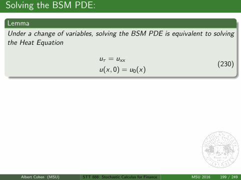
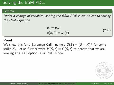
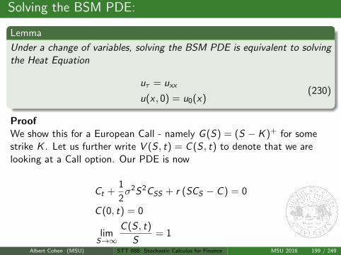
Solving the BSM PDE:
Lemma
Under a change of variables, solving the BSM PDE is equivalent to solvingthe Heat Equation
uτ = uxx
u(x , 0) = u0(x)(230)
ProofWe show this for a European Call - namely G (S) = (S − K )+ for somestrike K . Let us further write V (S , t) = C (S , t) to denote that we arelooking at a Call option. Our PDE is now
Ct +1
2σ2S2CSS + r (SCS − C ) = 0
C (0, t) = 0
limS→∞
C (S , t)
S= 1
C (S ,T ) = (S − K )+Albert Cohen (MSU) STT 888: Stochastic Calculus for Finance MSU 2016 199 / 249

Solving the BSM PDE:
Assume the change of variables
S = Kex
t = T − 1
2σ2τ
C (S , t) = Kv(x , τ)
(231)
and so
vτ = vxx +
(2r
σ2− 1
)vx −
2r
σ2v
Kv(x , 0) = max(Kex − K , 0)⇒ v(x , 0) = max(ex − 1, 0)
(232)
Furthermore, assume v(x , τ) = eαx+βτu(x , τ).
Albert Cohen (MSU) STT 888: Stochastic Calculus for Finance MSU 2016 200 / 249
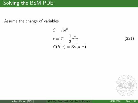
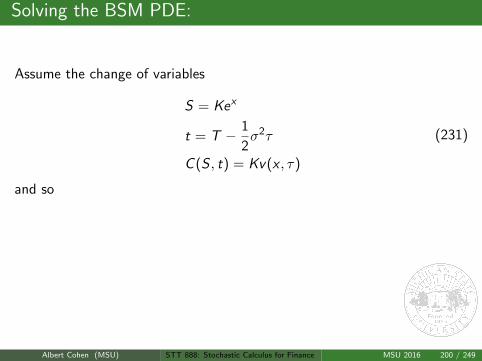
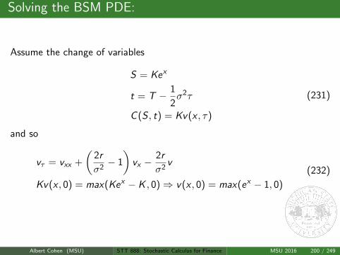
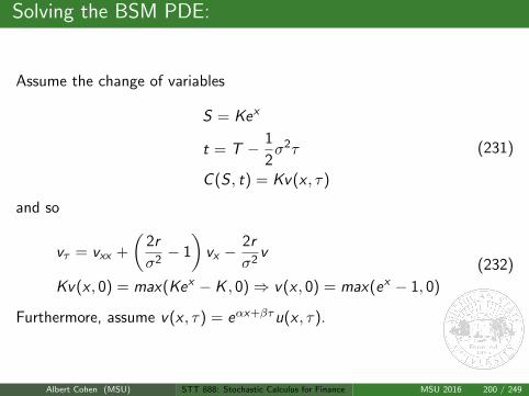
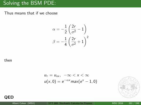
Solving the BSM PDE:
Thus means that if we choose
α = −1
2
(2r
σ2− 1
)β = −1
4
(2r
σ2+ 1
)2
then
uτ = uxx , −∞ < x <∞u(x , 0) = e−αxmax(ex − 1, 0)
QEDAlbert Cohen (MSU) STT 888: Stochastic Calculus for Finance MSU 2016 201 / 249

Solving the BSM PDE:
Question - How do we solve for u(x , τ)?
Answer - depends!
Try solving the following basic problem on the half real line:
uτ = uxx , x ≥ 0
u(0, τ) = 1
with the basic guess that we can reduce to an ordinary differentialequation via the transformation
ζ :=x√τ
(233)
and the solution u(x , τ) = U(ζ)
Albert Cohen (MSU) STT 888: Stochastic Calculus for Finance MSU 2016 202 / 249
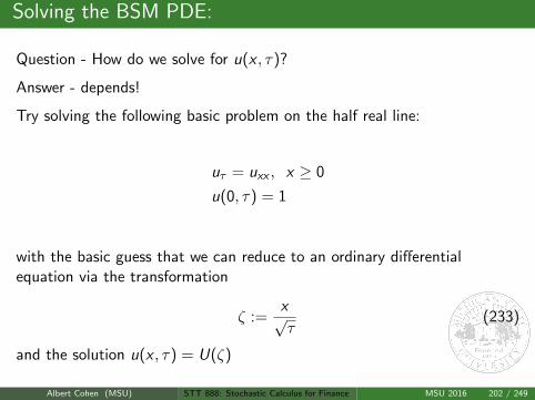

General Solution of Heat Equation
The resulting ODE is
U ′′(ζ) = −1
2ζU ′(ζ)
U(0) = 1
U(∞) = 0
which has solution
U(ζ) = C
∫ ζ
0e−
s2
4 ds + D (234)
which, upon satisfaction of the boundary conditions at 0 and ∞ leads to
U(ζ) =1√π
∫ ∞ζ
e−s2
4 ds ⇒ u(x , τ) =1√π
∫ ∞x√τ
e−s2
4 ds (235)
Albert Cohen (MSU) STT 888: Stochastic Calculus for Finance MSU 2016 203 / 249
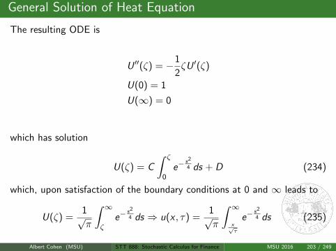

General Solution of Heat Equation
Again for the basic equation
uτ = uxx ∀x ∈ (−∞,∞) (236)
we look for solutions of the form
u(x , τ) =1√τ
U(ζ)
ζ :=x√τ
which leads to the ODE of the form
d
dζ
[U ′(ζ) +
1
2ζU(ζ)
]= 0 (237)
Albert Cohen (MSU) STT 888: Stochastic Calculus for Finance MSU 2016 204 / 249
General Solution of Heat Equation
Again for the basic equation
uτ = uxx ∀x ∈ (−∞,∞) (236)
we look for solutions of the form
u(x , τ) =1√τ
U(ζ)
ζ :=x√τ
which leads to the ODE of the form
d
dζ
[U ′(ζ) +
1
2ζU(ζ)
]= 0 (237)
Albert Cohen (MSU) STT 888: Stochastic Calculus for Finance MSU 2016 204 / 249
General Solution of Heat Equation
Again for the basic equation
uτ = uxx ∀x ∈ (−∞,∞) (236)
we look for solutions of the form
u(x , τ) =1√τ
U(ζ)
ζ :=x√τ
which leads to the ODE of the form
d
dζ
[U ′(ζ) +
1
2ζU(ζ)
]= 0 (237)
Albert Cohen (MSU) STT 888: Stochastic Calculus for Finance MSU 2016 204 / 249
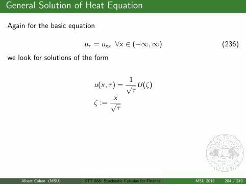
General Solution of Heat Equation
Again for the basic equation
uτ = uxx ∀x ∈ (−∞,∞) (236)
we look for solutions of the form
u(x , τ) =1√τ
U(ζ)
ζ :=x√τ
which leads to the ODE of the form
d
dζ
[U ′(ζ) +
1
2ζU(ζ)
]= 0 (237)
Albert Cohen (MSU) STT 888: Stochastic Calculus for Finance MSU 2016 204 / 249
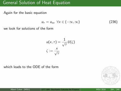
General Solution of Heat Equation
Again for the basic equation
uτ = uxx ∀x ∈ (−∞,∞) (236)
we look for solutions of the form
u(x , τ) =1√τ
U(ζ)
ζ :=x√τ
which leads to the ODE of the form
d
dζ
[U ′(ζ) +
1
2ζU(ζ)
]= 0 (237)
Albert Cohen (MSU) STT 888: Stochastic Calculus for Finance MSU 2016 204 / 249

General Solution of Heat Equation
Again for the basic equation
uτ = uxx ∀x ∈ (−∞,∞) (236)
we look for solutions of the form
u(x , τ) =1√τ
U(ζ)
ζ :=x√τ
which leads to the ODE of the form
d
dζ
[U ′(ζ) +
1
2ζU(ζ)
]= 0 (237)
Albert Cohen (MSU) STT 888: Stochastic Calculus for Finance MSU 2016 204 / 249

General Solution of Heat Equation
from which we take the fundamental solution
U(ζ) =1
2√π
e−ζ2
4
u(x , τ) =1
2√πτ
e−x2
4τ =: Γ(x , τ)
(238)
Now, consider the family of functions δε(x), parametrized by ε > 0, with
δε(x) :=1
2ε1[−ε,ε](x) (239)
It follows that
limε→0
∫ ∞−∞
δε(x)φ(x)dx = φ(0) (240)
for any reasonable function φ(x)
Albert Cohen (MSU) STT 888: Stochastic Calculus for Finance MSU 2016 205 / 249
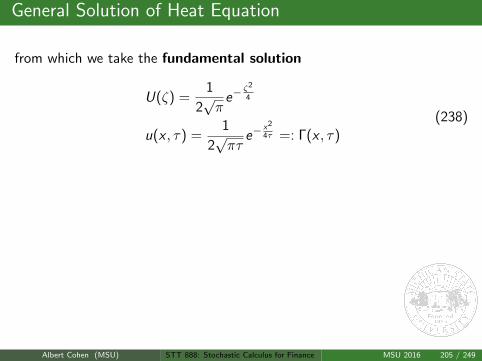
General Solution of Heat Equation
In general,
limε→0
∫ ∞−∞
δε(x − x0)φ(x)dx = φ(x0) (241)
We call the (weak) limit of δε(x) the Dirac delta δ(x), after the physicist.
Albert Cohen (MSU) STT 888: Stochastic Calculus for Finance MSU 2016 206 / 249
General Solution of Heat Equation
So, for any function u0(x), we have the relation
limε→0
∫ ∞−∞
δε(y − x)u0(y)dx = u0(x) (242)
It also follows that our fundamental solution Γ(x , τ)⇒ δ(x) as τ → 0.Since u(x , 0)” = ”δ(x) and Γ(x − s, τ) = Γ(s − x , τ) for fixed s, we have
∂
∂τ[u0(s)Γ(s − x , τ)] =
∂2
∂x2[u0(s)Γ(s − x , τ)]
u0(s)Γ(s − x , 0) = u0(s)δ(s − x)
(243)
Albert Cohen (MSU) STT 888: Stochastic Calculus for Finance MSU 2016 207 / 249
General Solution of Heat Equation
So, for any function u0(x), we have the relation
limε→0
∫ ∞−∞
δε(y − x)u0(y)dx = u0(x) (242)
It also follows that our fundamental solution Γ(x , τ)⇒ δ(x) as τ → 0.
Since u(x , 0)” = ”δ(x) and Γ(x − s, τ) = Γ(s − x , τ) for fixed s, we have
∂
∂τ[u0(s)Γ(s − x , τ)] =
∂2
∂x2[u0(s)Γ(s − x , τ)]
u0(s)Γ(s − x , 0) = u0(s)δ(s − x)
(243)
Albert Cohen (MSU) STT 888: Stochastic Calculus for Finance MSU 2016 207 / 249
General Solution of Heat Equation
So, for any function u0(x), we have the relation
limε→0
∫ ∞−∞
δε(y − x)u0(y)dx = u0(x) (242)
It also follows that our fundamental solution Γ(x , τ)⇒ δ(x) as τ → 0.Since u(x , 0)” = ”δ(x) and Γ(x − s, τ) = Γ(s − x , τ) for fixed s, we have
∂
∂τ[u0(s)Γ(s − x , τ)] =
∂2
∂x2[u0(s)Γ(s − x , τ)]
u0(s)Γ(s − x , 0) = u0(s)δ(s − x)
(243)
Albert Cohen (MSU) STT 888: Stochastic Calculus for Finance MSU 2016 207 / 249
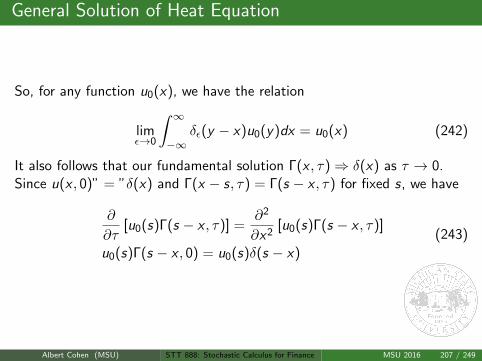

General Solution of Heat Equation
Since
u0(x) =
∫ ∞−∞
u0(s)δ(s − x)ds (244)
and u0(x)u(s − x , τ) is a solution of the PDE for all s, we have that
v(x , τ) =
∫ ∞−∞
u0(s)u(s − x , τ)ds
=
∫ ∞−∞
u0(s)1
2√πτ
e−(s−x)2
4τ ds
(245)
is a solution of
vτ = vxx
v(x , 0) = u0(x)(246)
Albert Cohen (MSU) STT 888: Stochastic Calculus for Finance MSU 2016 208 / 249
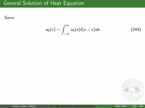
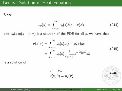
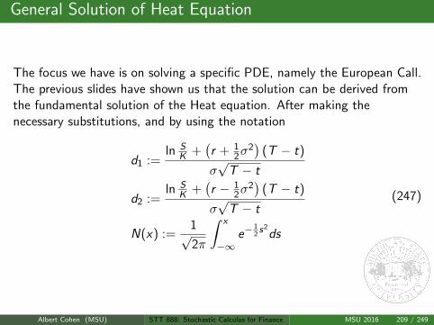
General Solution of Heat Equation
The focus we have is on solving a specific PDE, namely the European Call.The previous slides have shown us that the solution can be derived fromthe fundamental solution of the Heat equation. After making thenecessary substitutions, and by using the notation
d1 :=ln S
K +(r + 1
2σ2)
(T − t)
σ√
T − t
d2 :=ln S
K +(r − 1
2σ2)
(T − t)
σ√
T − t
N(x) :=1√2π
∫ x
−∞e−
12s2
ds
(247)
Albert Cohen (MSU) STT 888: Stochastic Calculus for Finance MSU 2016 209 / 249
General Solution of BSM PDE revisited
Then we have the closed form solution
C (S , t) = SN(d1)− Ke−r(T−t)N(d2) (248)
HW1: Can we use any theorems/ideas to use this work to find thecorresponding value of a European Put option without resorting to solvingthe associated PDE?
HW2: Prove that ∆C = ∂C∂S = N(d1)
HW3: Find the value of an option that pays 1 if the stock value is aboveK at time T , and 0 otherwise. Hint - use the above analysis!
Albert Cohen (MSU) STT 888: Stochastic Calculus for Finance MSU 2016 210 / 249
Black Scholes Pricing using Underlying Asset
In the next section, we will derive the following solutions to theBlack-Scholes PDE:
V C (S , t) = e−r(T−t)E [(ST − K )+ | St = S ]
= Se−δ(T−t)N(d1)− Ke−r(T−t)N(d2)
V P(S , t) = e−r(T−t)E [(K − ST )+ | St = S ]
= Ke−r(T−t)N(−d2)− Se−δ(T−t)N(−d1)
d1 =ln(
SK
)+ (r − δ + 1
2σ2)(T − t)
σ√
T − t
d2 = d1 − σ√
T − t
N(x) =1√2π
∫ x
−∞e−
z2
2 dz .
(249)
Notice that V C (S , t)− V P(S , t) = Se−δ(T−t) − Ke−r(T−t).Question: What underlying model of stock evolution leads to this value?How can we support such a probability measure?
Albert Cohen (MSU) STT 888: Stochastic Calculus for Finance MSU 2016 211 / 249
Normal Random Variables
We say that X is a Normal Random Variable with parameters µ, σ2 if
fX (x) =1√2πσ
e−(x−µ)2
2σ2 for −∞ < x <∞ (250)
Furthermore, we say that Z is a Standard Normal Random Variable if it isNormal with parameters µ = 0, σ = 1. Consider
z =x − µσ∫ ∞
−∞fX (x)dx =
∫ ∞−∞
1√2πσ
e−(x−µ)2
2σ2 dx
=
∫ ∞−∞
1√2π
e−(z)2
2 dz
=
∫ ∞−∞
fZ (z)dz
(251)
Albert Cohen (MSU) STT 888: Stochastic Calculus for Finance MSU 2016 212 / 249
Normal Random Variables
We user the notation X ∼ N(µ, σ2) and Z ∼ N(0, 1). By ourtransformation above, it can be seen that if Z ∼ N(0, 1), thenX = µ+ σ · Z ∼ N(µ, σ2). We can see this via
Φ(z) := FZ (z) = P[Z ≤ z ]
= P[X − µσ
≤ x − µσ
]
= P[X ≤ x ] =: FX (x)
1
σfZ
(x − µσ
)=
d
dxFZ (z)
=d
dxFX (x) = fX (x)
fZ (z) =1√2π
e−(z)2
2
(252)
Albert Cohen (MSU) STT 888: Stochastic Calculus for Finance MSU 2016 213 / 249
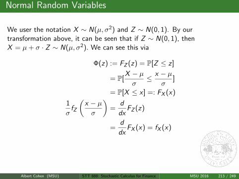
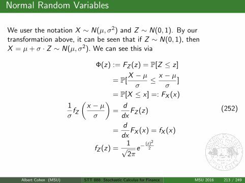
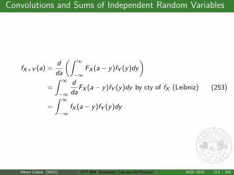
Convolutions and Sums of Independent Random Variables
fX+Y (a) =d
da
(∫ ∞−∞
FX (a− y)fY (y)dy
)=
∫ ∞−∞
d
daFX (a− y)fY (y)dy by cty of fX (Leibniz)
=
∫ ∞−∞
fX (a− y)fY (y)dy
(253)
Albert Cohen (MSU) STT 888: Stochastic Calculus for Finance MSU 2016 214 / 249
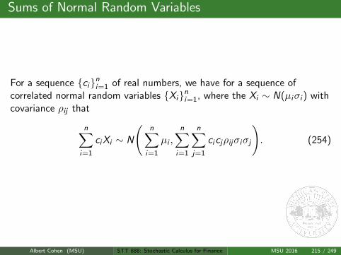
Sums of Normal Random Variables
For a sequence cini=1 of real numbers, we have for a sequence ofcorrelated normal random variables Xini=1, where the Xi ∼ N(µiσi ) withcovariance ρij that
n∑i=1
ciXi ∼ N
(n∑
i=1
µi ,
n∑i=1
n∑j=1
cicjρijσiσj
). (254)
Albert Cohen (MSU) STT 888: Stochastic Calculus for Finance MSU 2016 215 / 249
Lognormal Random Variables
We say that Y ∼ LN(µ, σ) is Lognormal if ln(Y ) ∼ N(µ, σ2).
As sums of normal random variables remain normal, products of lognormalrandom variables remain lognormal.
Recall that the moment-generating function ofX ∼ N(µ, σ2) ∼ µ+ σN(0, 1) is
MX (t) = E[etX ] = eµt+ 12σ2t2
(255)
If Y = eµ+σZ , then, it can be seen that
E[Y n] = E[enX ] = eµn+ 12σ2n2
(256)
and
fY (y) =1
σ√
2πyexp
(− (ln(y)− µ)2
2σ2
)(257)
Albert Cohen (MSU) STT 888: Stochastic Calculus for Finance MSU 2016 216 / 249
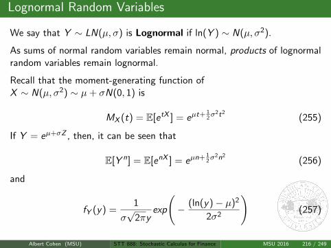
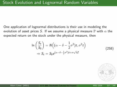
Stock Evolution and Lognormal Random Variables
One application of lognormal distributions is their use in modeling theevolution of asset prices S . If we assume a physical measure P with α theexpected return on the stock under the physical measure, then
ln
(St
S0
)= N
((α− δ − 1
2σ2)t, σ2t
)⇒ St = S0e(α−δ− 1
2σ2)t+σ
√tZ
(258)
Albert Cohen (MSU) STT 888: Stochastic Calculus for Finance MSU 2016 217 / 249
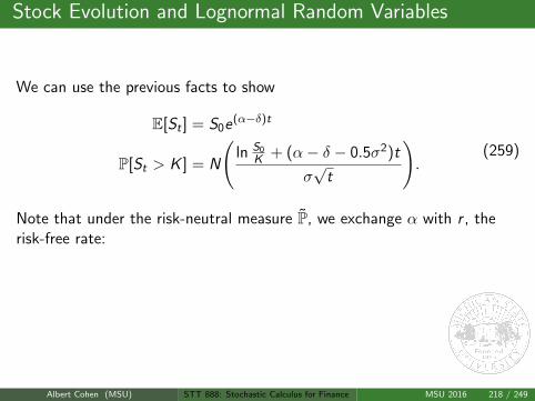
Stock Evolution and Lognormal Random Variables
We can use the previous facts to show
E[St ] = S0e(α−δ)t
P[St > K ] = N
(ln S0
K + (α− δ − 0.5σ2)t
σ√
t
).
(259)
Note that under the risk-neutral measure P, we exchange α with r , therisk-free rate:
E[St ] = S0e(r−δ)t
P[St > K ] = N(d2).(260)
Albert Cohen (MSU) STT 888: Stochastic Calculus for Finance MSU 2016 218 / 249
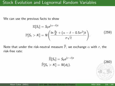
Stock Evolution and Lognormal Random Variables
The next challenge is to construct a process St that possesses the aboveproperties as well as continuity of paths.
Click here for a neat article relating actuarial reserving to option pricing!
Albert Cohen (MSU) STT 888: Stochastic Calculus for Finance MSU 2016 219 / 249
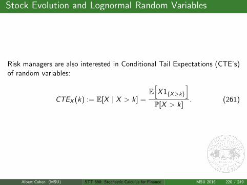
Stock Evolution and Lognormal Random Variables
Risk managers are also interested in Conditional Tail Expectations (CTE’s)of random variables:
CTEX (k) := E[X | X > k] =E[X 1X>k
]P[X > k]
. (261)
Albert Cohen (MSU) STT 888: Stochastic Calculus for Finance MSU 2016 220 / 249
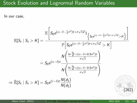
Stock Evolution and Lognormal Random Variables
In our case,
E[St | St > K ] =
E
[S0e(α−δ− 1
2σ2)t+σ
√tZ1
S0e(α−δ− 1
2σ2)t+σ
√tZ>K
]
P[S0e(α−δ− 1
2σ2)t+σ
√tZ > K
]
= S0e(α−δ)t
N
(ln
S0K
+(α−δ+0.5σ2)t
σ√t
)
N
(ln
S0K
+(α−δ−0.5σ2)t
σ√t
)
⇒ E[St | St > K ] = S0e(r−δ)t N(d1)
N(d2)(262)
Albert Cohen (MSU) STT 888: Stochastic Calculus for Finance MSU 2016 221 / 249
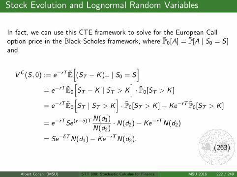
Stock Evolution and Lognormal Random Variables
In fact, we can use this CTE framework to solve for the European Calloption price in the Black-Scholes framework, where P0[A] = P[A | S0 = S ]and
V C (S , 0) := e−rT E[(ST − K )+ | S0 = S
]= e−rT E0
[ST − K | ST > K
]· P0[ST > K ]
= e−rT E0
[ST | ST > K
]· P0[ST > K ]− Ke−rT P0[ST > K ]
= e−rTSe(r−δ)T N(d1)
N(d2)· N(d2)− Ke−rTN(d2)
= Se−δTN(d1)− Ke−rTN(d2).(263)
Albert Cohen (MSU) STT 888: Stochastic Calculus for Finance MSU 2016 222 / 249
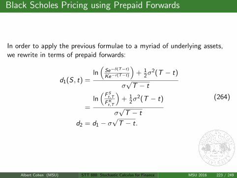
Black Scholes Pricing using Prepaid Forwards
In order to apply the previous formulae to a myriad of underlying assets,we rewrite in terms of prepaid forwards:
d1(S , t) =ln(Se−δ(T−t)
Ke−r(T−t)
)+ 1
2σ2(T − t)
σ√
T − t
=ln(F St,T
FKt,T
)+ 1
2σ2(T − t)
σ√
T − t
d2 = d1 − σ√
T − t.
(264)
Albert Cohen (MSU) STT 888: Stochastic Calculus for Finance MSU 2016 223 / 249
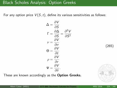
Black Scholes Analysis: Option Greeks
For any option price V (S , t), define its various sensitivities as follows:
∆ =∂V
∂S
Γ =∂∆
∂S=∂2V
∂S2
ν =∂V
∂σ
Θ =∂V
∂t
ρ =∂V
∂r
Ψ =∂V
∂δ.
(265)
These are known accordingly as the Option Greeks.
Albert Cohen (MSU) STT 888: Stochastic Calculus for Finance MSU 2016 224 / 249
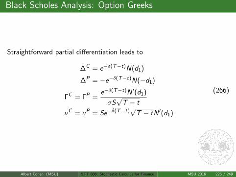
Black Scholes Analysis: Option Greeks
Straightforward partial differentiation leads to
∆C = e−δ(T−t)N(d1)
∆P = −e−δ(T−t)N(−d1)
ΓC = ΓP =e−δ(T−t)N ′(d1)
σS√
T − t
νC = νP = Se−δ(T−t)√
T − tN ′(d1)
(266)
Albert Cohen (MSU) STT 888: Stochastic Calculus for Finance MSU 2016 225 / 249
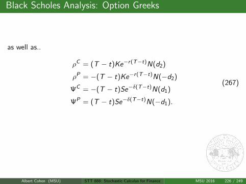
Black Scholes Analysis: Option Greeks
as well as..
ρC = (T − t)Ke−r(T−t)N(d2)
ρP = −(T − t)Ke−r(T−t)N(−d2)
ΨC = −(T − t)Se−δ(T−t)N(d1)
ΨP = (T − t)Se−δ(T−t)N(−d1).
(267)
What do the signs of the Greeks tell us?
HW: Compute Θ for puts and calls.
Albert Cohen (MSU) STT 888: Stochastic Calculus for Finance MSU 2016 226 / 249
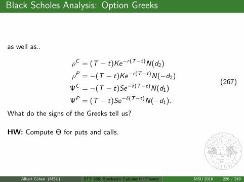
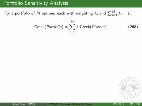
Portfolio Sensitivity Analysis
For a portfolio of M options, each with weighting λi and∑M
i=1 λi = 1:
Greek(Portfolio) =M∑i=1
λiGreek(i thasset). (268)
If P(i) is the price of a portfolio of income streams: P(i) =∑n
k=1 Pk(i).
⇒ D = −(1 + i) · P ′(i)
P(i)= −(1 + i) ·
∑nk=1 P ′k(i)
P(i)
= −(1 + i) ·n∑
k=1
P ′k(i)
P(i)= −(1 + i) ·
n∑k=1
Pk(i)
P(i)·
P ′k(i)
Pk(i)
=n∑
k=1
Dk · qk
(269)
and so the portfolio duration is the weighted average of the individualdurations. What if the interest rate i is a random variable itself?
Albert Cohen (MSU) STT 888: Stochastic Calculus for Finance MSU 2016 227 / 249
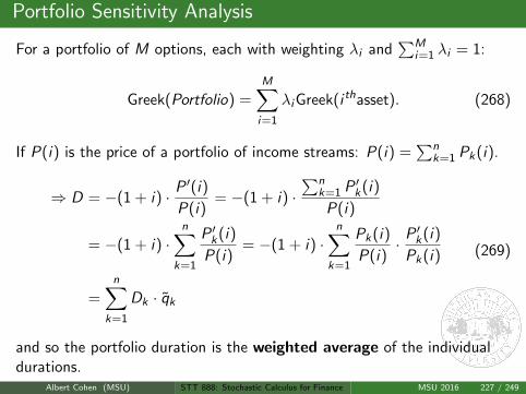
Portfolio Sensitivity Analysis
For a portfolio of M options, each with weighting λi and∑M
i=1 λi = 1:
Greek(Portfolio) =M∑i=1
λiGreek(i thasset). (268)
If P(i) is the price of a portfolio of income streams: P(i) =∑n
k=1 Pk(i).
⇒ D = −(1 + i) · P ′(i)
P(i)= −(1 + i) ·
∑nk=1 P ′k(i)
P(i)
= −(1 + i) ·n∑
k=1
P ′k(i)
P(i)= −(1 + i) ·
n∑k=1
Pk(i)
P(i)·
P ′k(i)
Pk(i)
=n∑
k=1
Dk · qk
(269)
and so the portfolio duration is the weighted average of the individualdurations.
What if the interest rate i is a random variable itself?
Albert Cohen (MSU) STT 888: Stochastic Calculus for Finance MSU 2016 227 / 249
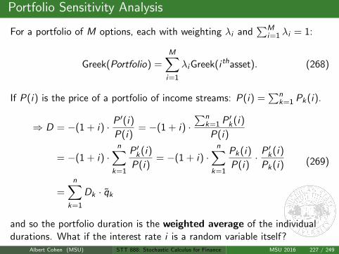
Portfolio Sensitivity Analysis
For a portfolio of M options, each with weighting λi and∑M
i=1 λi = 1:
Greek(Portfolio) =M∑i=1
λiGreek(i thasset). (268)
If P(i) is the price of a portfolio of income streams: P(i) =∑n
k=1 Pk(i).
⇒ D = −(1 + i) · P ′(i)
P(i)= −(1 + i) ·
∑nk=1 P ′k(i)
P(i)
= −(1 + i) ·n∑
k=1
P ′k(i)
P(i)= −(1 + i) ·
n∑k=1
Pk(i)
P(i)·
P ′k(i)
Pk(i)
=n∑
k=1
Dk · qk
(269)
and so the portfolio duration is the weighted average of the individualdurations. What if the interest rate i is a random variable itself?
Albert Cohen (MSU) STT 888: Stochastic Calculus for Finance MSU 2016 227 / 249
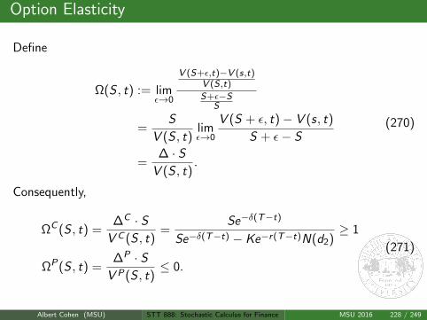
Option Elasticity
Define
Ω(S , t) := limε→0
V (S+ε,t)−V (s,t)V (S,t)
S+ε−SS
=S
V (S , t)limε→0
V (S + ε, t)− V (s, t)
S + ε− S
=∆ · S
V (S , t).
(270)
Consequently,
ΩC (S , t) =∆C · S
V C (S , t)=
Se−δ(T−t)
Se−δ(T−t) − Ke−r(T−t)N(d2)≥ 1
ΩP(S , t) =∆P · S
V P(S , t)≤ 0.
(271)
Albert Cohen (MSU) STT 888: Stochastic Calculus for Finance MSU 2016 228 / 249
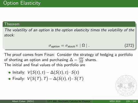
Option Elasticity
Theorem
The volatility of an option is the option elasticity times the volatility of thestock:
σoption = σstock× | Ω | . (272)
The proof comes from Finan: Consider the strategy of hedging a portfolioof shorting an option and purchasing ∆ = ∂V
∂S shares.The initial and final values of this portfolio are
Initally: V (S(t), t)−∆(S(t), t) · S(t)
Finally: V (S(T ),T )−∆(S(t), t) · S(T )
Albert Cohen (MSU) STT 888: Stochastic Calculus for Finance MSU 2016 229 / 249
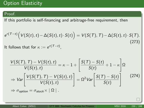
Option Elasticity
Proof.
If this portfolio is self-financing and arbitrage-free requirement, then
er(T−t)(
V (S(t), t)−∆(S(t), t) ·S(t))
= V (S(T ),T )−∆(S(t), t) ·S(T ).
(273)It follows that for κ := er(T−t),
V (S(T ),T )− V (S(t), t)
V (S(t), t)= κ− 1 +
[S(T )− S(t)
S(t)+ 1− κ
]Ω
⇒ Var
[V (S(T ),T )− V (S(t), t)
V (S(t), t)
]= Ω2Var
[S(T )− S(t)
S(t)
]⇒ σoption = σstock× | Ω | .
(274)
Albert Cohen (MSU) STT 888: Stochastic Calculus for Finance MSU 2016 230 / 249
Option Elasticity
If γ is the expected rate of return on an option with value V , α is theexpected rate of return on the underlying stock, and r is of course the riskfree rate, then the following equation holds:
γ · V (S , t) = α ·∆(S , t) · S + r ·(
V (S , t)−∆(S , t) · S). (275)
In terms of elasticity Ω, this reduces to
Risk Premium(Option) := γ − r = (α− r)Ω. (276)
Furthermore, we have the Sharpe Ratio for an asset as the ratio of riskpremium to volatility:
Sharpe(Stock) =(α− r)
σ=
(α− r)Ω
σΩ= Sharpe(Call). (277)
HW Sharpe Ratio for a put? How about elasticity for a portfolio ofoptions? Now read about Calendar Spreads, Implied Volatility, andPerpetual American Options.
Albert Cohen (MSU) STT 888: Stochastic Calculus for Finance MSU 2016 231 / 249
Example: Hedging
Under a standard framework, assume you write a 4− yr European Calloption a non-dividend paying stock with the following:
S0 = 10 = K
σ = 0.2
r = 0.02.
(278)
Calculate the initial number of shares of the stock for your hedgingprogram.
Albert Cohen (MSU) STT 888: Stochastic Calculus for Finance MSU 2016 232 / 249
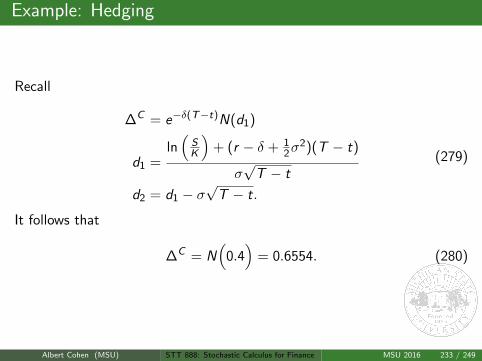
Example: Hedging
Recall
∆C = e−δ(T−t)N(d1)
d1 =ln(
SK
)+ (r − δ + 1
2σ2)(T − t)
σ√
T − t
d2 = d1 − σ√
T − t.
(279)
It follows that
∆C = N(
0.4)
= 0.6554. (280)
Albert Cohen (MSU) STT 888: Stochastic Calculus for Finance MSU 2016 233 / 249
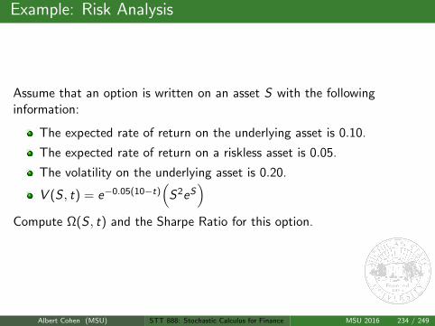
Example: Risk Analysis
Assume that an option is written on an asset S with the followinginformation:
The expected rate of return on the underlying asset is 0.10.
The expected rate of return on a riskless asset is 0.05.
The volatility on the underlying asset is 0.20.
V (S , t) = e−0.05(10−t)(
S2eS)
Compute Ω(S , t) and the Sharpe Ratio for this option.
Albert Cohen (MSU) STT 888: Stochastic Calculus for Finance MSU 2016 234 / 249
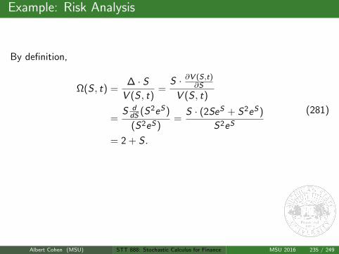
Example: Risk Analysis
By definition,
Ω(S , t) =∆ · S
V (S , t)=
S · ∂V (S,t)∂S
V (S , t)
=S d
dS (S2eS)
(S2eS)=
S · (2SeS + S2eS)
S2eS
= 2 + S .
(281)
Furthermore, since Ω = 2 + S ≥ 2, we have
Sharpe =0.10− 0.05
0.20= 0.25. (282)
Albert Cohen (MSU) STT 888: Stochastic Calculus for Finance MSU 2016 235 / 249
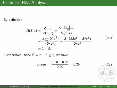
Example: Black Scholes Pricing
Consider a portfolio of options on a non-dividend paying stock S thatconsists of a put and a call, both with strike K = 5 = S0. What is the Γfor this option as well as the option value at time 0 if the time toexpiration is T = 4, r = 0.02, σ = 0.2.
In this case,
V = V C + V P
Γ =∂2
∂S2
(V C + V P
)= 2ΓC .
(283)
Albert Cohen (MSU) STT 888: Stochastic Calculus for Finance MSU 2016 236 / 249
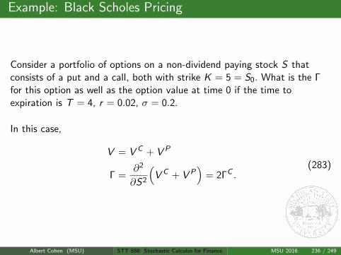
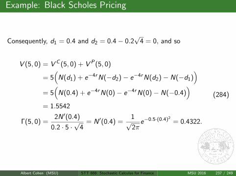
Example: Black Scholes Pricing
Consequently, d1 = 0.4 and d2 = 0.4− 0.2√
4 = 0, and so
V (5, 0) = V C (5, 0) + V P(5, 0)
= 5(
N(d1) + e−4rN(−d2)− e−4rN(d2)− N(−d1))
= 5(
N(0.4) + e−4rN(0)− e−4rN(0)− N(−0.4))
= 1.5542
Γ(5, 0) =2N ′(0.4)
0.2 · 5 ·√
4= N ′(0.4) =
1√2π
e−0.5·(0.4)2= 0.4322.
(284)
Albert Cohen (MSU) STT 888: Stochastic Calculus for Finance MSU 2016 237 / 249
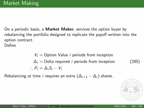
Market Making
On a periodic basis, a Market Maker, services the option buyer byrebalancing the portfolio designed to replicate the payoff written into theoption contract.Define
Vi = Option Value i periods from inception
∆i = Delta required i periods from inception
∴ Pi = ∆iSi − Vi
(285)
Rebalancing at time i requires an extra (∆i+1 −∆i ) shares.
Albert Cohen (MSU) STT 888: Stochastic Calculus for Finance MSU 2016 238 / 249
Market Making
On a periodic basis, a Market Maker, services the option buyer byrebalancing the portfolio designed to replicate the payoff written into theoption contract.Define
Vi = Option Value i periods from inception
∆i = Delta required i periods from inception
∴ Pi = ∆iSi − Vi = Cost of Strategy
(286)
Rebalancing at time i requires an extra (∆i+1 −∆i ) shares.
Albert Cohen (MSU) STT 888: Stochastic Calculus for Finance MSU 2016 239 / 249
Market Making
Define
∂Si = Si+1 − Si
∂Pi = Pi+1 − Pi
∂∆i = ∆i+1 −∆i
(287)
Then
∂Pi = Net Cash Flow = ∆i∂Si − ∂Vi − rPi
= ∆i∂Si − ∂Vi − r(
∆iSi − Vi
) (288)
Under what conditions is the Net Flow = 0?
Albert Cohen (MSU) STT 888: Stochastic Calculus for Finance MSU 2016 240 / 249
Market Making
For a continuous rate r , we can see that if ∆ := ∂V∂S , Pt = ∆tSt − Vt ,
dV := V (St + dSt , t + dt)− V (St , t)
≈ Θdt + ∆ · dSt +1
2Γ · (dSt)
2
⇒ dPt = ∆tdSt − dVt − rPtdt
≈ ∆tdSt −(
Θdt + ∆ · dSt +1
2Γ · (dSt)
2
)− r (∆tSt − Vt) dt
≈ −
(Θdt + r(∆St − V (St , t))dt +
1
2Γ · [dSt ]
2
).
(289)
Albert Cohen (MSU) STT 888: Stochastic Calculus for Finance MSU 2016 241 / 249
Market Making
If dt is small, but not infinitessimally small, then on a periodic basis giventhe evolution of St , the periodic jump in value from St → St + dSt may beknown exactly and correspond to a non-zero jump in Market Maker profitdPt .
If dSt · dSt = σ2S2t dt, then if we sample continuously and enforce a zero
net-flow, we retain the BSM PDE for all relevant (S , t):
∂V
∂t+ r(
S∂V
∂S− V
)+
1
2σ2S2∂
2V
∂S2= 0
V (S ,T ) = G (S) for final time payoff G (S).
(290)
Albert Cohen (MSU) STT 888: Stochastic Calculus for Finance MSU 2016 242 / 249
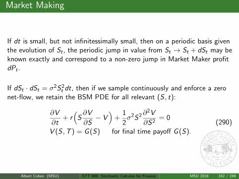
Note: Delta-Gamma Neutrality vs Bond Immunization
In an actuarial analysis of cashflow, a company may wish to immunizeits portfolio. This refers to the relationship between a non-zero valuefor the second derivative with respect to interest rate of the(deterministic) cashflow present value and the subsequent possibilityof a negative PV.
This is similar to the case of market maker with a non-zero Gamma.In the market makers cash flow, a move of dS in the stockcorresponds to a move 1
2 Γ(dS)2 in the portfolio value.
In order to protect against large swings in the stock causing non-lineareffects in the portfolio value, the market maker may choose to offsetpositions in her present holdings to maintain Gamma Neutrality or shewish to maintain Delta Neutrality, although this is only a linear effect.
Albert Cohen (MSU) STT 888: Stochastic Calculus for Finance MSU 2016 243 / 249
Option Greeks and Analysis - Some Final Comments
It is important to note the similarities between Market Making andActuarial Reserving. In engineering the portfolio to replicate thepayoff written into the contract, the market maker requires capital.
The idea of Black Scholes Merton pricing is that the portfolio shouldbe self-financing.
One should consider how this compares with the capital required byinsurers to maintain solvency as well as the possibility of obtainingreinsurance.
Albert Cohen (MSU) STT 888: Stochastic Calculus for Finance MSU 2016 244 / 249
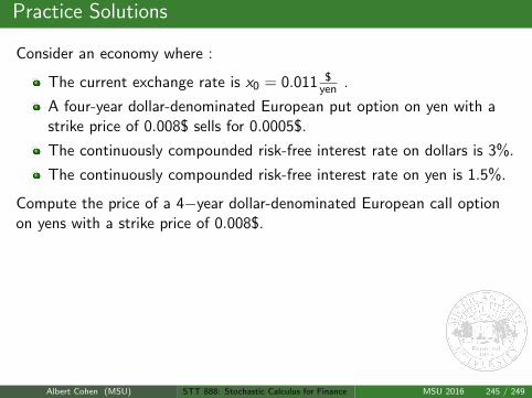
Practice Solutions
Consider an economy where :
The current exchange rate is x0 = 0.011 $yen .
A four-year dollar-denominated European put option on yen with astrike price of 0.008$ sells for 0.0005$.
The continuously compounded risk-free interest rate on dollars is 3%.
The continuously compounded risk-free interest rate on yen is 1.5%.
Compute the price of a 4−year dollar-denominated European call optionon yens with a strike price of 0.008$.
ANSWER: By put call parity, and the Black Scholes formula, with theasset S as the exchange rate, and the foreign risk-free rate rf = δ,
V C (x0, 0) = V P(x0, 0) + x0e−rf T − Ke−rT
= 0.0005 + 0.011e−0.015·4 − 0.008e−0.03·4
= 0.003764.
(291)
Albert Cohen (MSU) STT 888: Stochastic Calculus for Finance MSU 2016 245 / 249
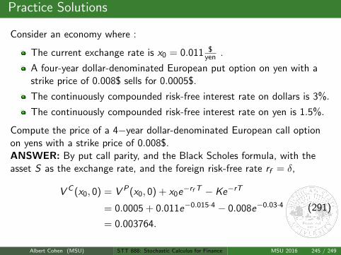
Practice Solutions
Consider an economy where :
The current exchange rate is x0 = 0.011 $yen .
A four-year dollar-denominated European put option on yen with astrike price of 0.008$ sells for 0.0005$.
The continuously compounded risk-free interest rate on dollars is 3%.
The continuously compounded risk-free interest rate on yen is 1.5%.
Compute the price of a 4−year dollar-denominated European call optionon yens with a strike price of 0.008$.ANSWER: By put call parity, and the Black Scholes formula, with theasset S as the exchange rate, and the foreign risk-free rate rf = δ,
V C (x0, 0) = V P(x0, 0) + x0e−rf T − Ke−rT
= 0.0005 + 0.011e−0.015·4 − 0.008e−0.03·4
= 0.003764.
(291)
Albert Cohen (MSU) STT 888: Stochastic Calculus for Finance MSU 2016 245 / 249
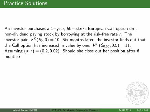
Practice Solutions
An investor purchases a 1−year, 50− strike European Call option on anon-dividend paying stock by borrowing at the risk-free rate r . Theinvestor paid V C (S0, 0) = 10. Six months later, the investor finds out thatthe Call option has increased in value by one: V C (S0.05, 0.5) = 11.Assuming (σ, r) = (0.2, 0.02). Should she close out her position after 6months?
ANSWER: Simply put, her profit if she closes out after 6 months is
11− 10e0.02 12 = 0.8995. (292)
So, yes, she should liquidate her position.
Albert Cohen (MSU) STT 888: Stochastic Calculus for Finance MSU 2016 246 / 249
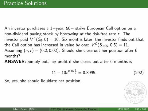
Practice Solutions
An investor purchases a 1−year, 50− strike European Call option on anon-dividend paying stock by borrowing at the risk-free rate r . Theinvestor paid V C (S0, 0) = 10. Six months later, the investor finds out thatthe Call option has increased in value by one: V C (S0.05, 0.5) = 11.Assuming (σ, r) = (0.2, 0.02). Should she close out her position after 6months?ANSWER: Simply put, her profit if she closes out after 6 months is
11− 10e0.02 12 = 0.8995. (292)
So, yes, she should liquidate her position.
Albert Cohen (MSU) STT 888: Stochastic Calculus for Finance MSU 2016 246 / 249
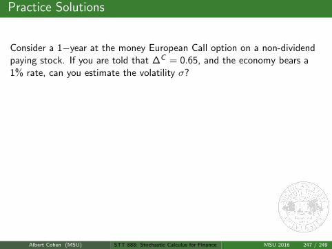
Practice Solutions
Consider a 1−year at the money European Call option on a non-dividendpaying stock. If you are told that ∆C = 0.65, and the economy bears a1% rate, can you estimate the volatility σ?
ANSWER: By definition,
∆C = e−δTN(d1) = N( r + 1
2σ2
σ
)= N
(0.01 + 12σ
2
σ
)= 0.65
⇒0.01 + 1
2σ2
σ= 0.385
⇒ σ ∈ 0.0269, 0.7431 .
(293)
More information is needed to choose from the two roots computed above.
Albert Cohen (MSU) STT 888: Stochastic Calculus for Finance MSU 2016 247 / 249
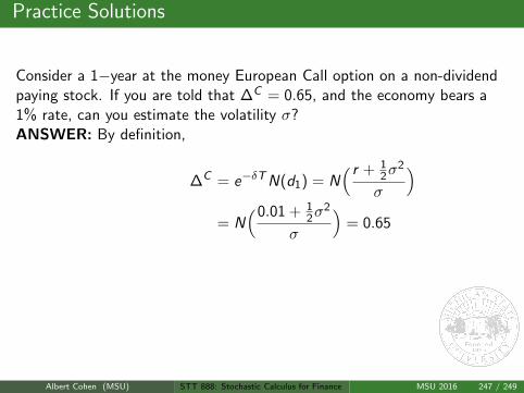
Practice Solutions
Consider a 1−year at the money European Call option on a non-dividendpaying stock. If you are told that ∆C = 0.65, and the economy bears a1% rate, can you estimate the volatility σ?ANSWER: By definition,
∆C = e−δTN(d1) = N( r + 1
2σ2
σ
)= N
(0.01 + 12σ
2
σ
)= 0.65
⇒0.01 + 1
2σ2
σ= 0.385
⇒ σ ∈ 0.0269, 0.7431 .
(293)
More information is needed to choose from the two roots computed above.
Albert Cohen (MSU) STT 888: Stochastic Calculus for Finance MSU 2016 247 / 249
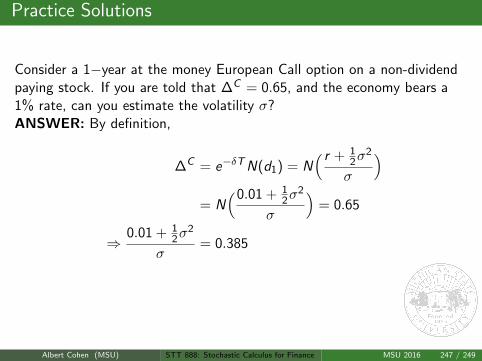
Practice Solutions
Consider a 1−year at the money European Call option on a non-dividendpaying stock. If you are told that ∆C = 0.65, and the economy bears a1% rate, can you estimate the volatility σ?ANSWER: By definition,
∆C = e−δTN(d1) = N( r + 1
2σ2
σ
)= N
(0.01 + 12σ
2
σ
)= 0.65
⇒0.01 + 1
2σ2
σ= 0.385
⇒ σ ∈ 0.0269, 0.7431 .
(293)
More information is needed to choose from the two roots computed above.
Albert Cohen (MSU) STT 888: Stochastic Calculus for Finance MSU 2016 247 / 249
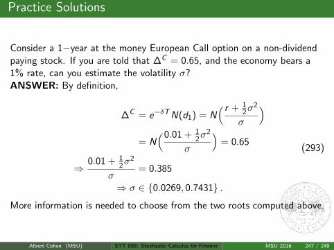
Practice Solutions
Consider a 1−year at the money European Call option on a non-dividendpaying stock. If you are told that ∆C = 0.65, and the economy bears a1% rate, can you estimate the volatility σ?ANSWER: By definition,
∆C = e−δTN(d1) = N( r + 1
2σ2
σ
)= N
(0.01 + 12σ
2
σ
)= 0.65
⇒0.01 + 1
2σ2
σ= 0.385
⇒ σ ∈ 0.0269, 0.7431 .
(293)
More information is needed to choose from the two roots computed above.
Albert Cohen (MSU) STT 888: Stochastic Calculus for Finance MSU 2016 247 / 249

Review
Are you comfortable with...
The definition of the Black-Scholes pricing formulae for Europeanputs and calls.
What are the Greeks? Given a specific option, could you compute theGreeks?
What is the Option Elasticity? How is it useful? How about theSharpe ratio of an option? Can you compute the Elasticity andSharpe ration of a given option?
Albert Cohen (MSU) STT 888: Stochastic Calculus for Finance MSU 2016 248 / 249
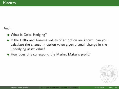
Review
And...
What is Delta Hedging?
If the Delta and Gamma values of an option are known, can youcalculate the change in option value given a small change in theunderlying asset value?
How does this correspond the Market Maker’s profit?
Albert Cohen (MSU) STT 888: Stochastic Calculus for Finance MSU 2016 249 / 249