SOME RECENT DEVELOPMENTS AND OPEN PROBLEMSIN SOLUTION METHODS FOR

MATHEMATICAL INVERSE PROBLEMS

Patricia K. Lamm – lamm@math.msu.eduDepartment of Mathematics, Michigan State University, East Lansing, MI 48824–1027USA. This work was supported in part by the National Science Foundation under con-tract number NSF DMS 9704899.

Abstract. The area of mathematical inverse problems is quite broad and involvesthe qualitative and quantitative analysis of a wide variety of physical models. Applica-tions include, for example, the problem of inverse heat conduction, image reconstruc-tion, tomography, the inverse scattering problem, and the determination of unknowncoefficients or boundary parameters appearing in partial differential equation models ofphysical phenomena.

We will survey some recent developments in the area of regularization methods formathematical inverse problems and indicate where further contributions are needed. Wewill discuss methods for which a primary goal is to avoid the oversmoothing of solutionsthat typically occurs when classical regularization schemes (such as Tikhonov regulariza-tion) are used. Oversmoothing is particularly troublesome in imaging and tomographicapplications, where it is of high priority to recover sharp or fine features of solutions. Wewill also explore the trend to design localized regularization methods which complementthe qualitative nature of a particular inverse problem (as opposed to the application of ageneric regularization method such as Tikhonov’s method). Local regularization methodstend to be more attractive in terms of numerical costs and implementation, but a numberof open questions remain in their theoretical analysis. Finally, we will discuss currentwork in the area of iterative solution methods, regularization schemes which have beensuccessfully applied to a number of important nonlinear inverse problems.

Key-words: mathematical inverse problems, regularization methods, iterative reg-ularization, local regularization methods, inverse heat conduction, imaging.

1. INTRODUCTION

The purpose of this paper is to survey some recent developments in the area ofregularization methods for mathematical inverse problems. In undertaking this taskit is difficult to avoid a certain amount of mathematical rigor. Nevertheless, becauseone goal of the paper is to try to explain some newer developments in mathematicalregularization theory to an audience which may not have the needed background coursesin operator theory or functional analysis, we will wherever possible try to use moreformal (less rigorous) explanations and to supplement the mathematical concepts belowwith examples. We will also take a few short-cuts in some definitions and statements ofthe theory in order to keep notation simplified and the level of mathematical expositionwithin reach of a more general audience. We do this with apologies to those readerswishing a more careful mathematical treatment of these topics (and who will recognizefairly quickly the short-cuts we have taken) and strongly encourage these readers toexplore the references given at the end of the paper.

Mathematically, an inverse problem is often expressed as the problem of finding u(a function, typically) which solves the operator equation

A(u) = f (1)

where f is an “idealized” data function. (Usually we require u ∈ X, a real Banach orreal Hilbert space, and we take f belonging to a real Hilbert space Y .) The operatorA may be linear or nonlinear, depending on the application; below we will give explicitdefinitions of A in the case of several important examples. If the data f is not in therange of A there is no possibility of a solution of (1), so typically we generalize theinverse problem and instead seek a solution u of the output least squares problem

J(u) = minu

J(u) (2)

whereJ(u)

def= ‖A(u)− f‖2

Y, (3)

for A the operator in (1) and for ‖·‖Y the norm used to measure data functions (i.e., thenorm on the Hilbert space Y ). For the latter, a common situation is where Y indicatesthe space of square-integrable functions on a given domain Ω; in this case, the norm‖ · ‖Y is defined via

‖A(u)− f‖2Y

=∫

Ω|A(u)(x)− f(x)|2 dx. (4)

It can be the case that there are many solutions of the output least squares problem;in this case, uniqueness can often be restored by seeking a minimum norm solution u ofthe least squares problem (see, e.g., [20, 28]).

An inverse problem is generally ill-posed in the sense that u does not depend continu-ously on f ; what this means in a practical setting is that whenever we only have in handan imprecise measurement f δ of the data (instead of the idealized f – in fact, this is thenormal situation due the usual presence of measurement error or computer round-offerror), then one cannot rely upon the solution uδ obtained by solving (1) (or (2)) using

2

the perturbed data f δ in place of f . That is, we generally have uδ far from u even if f δ

is close to f . Typically the presence of data error leads to highly oscillatory solutions,and this can only be avoided if a stabilization procedure or regularization method is used.

In what follows we give two examples of linear inverse problems, followed by oneexample of a nonlinear inverse problem; in each case we define the associated operatorA and we indicate what kind of finite-dimensional equations arise when discretizationmethods are applied to enable computer-based solution of each inverse problem.

Example 1. The inverse heat conduction problem (IHCP).The inverse heat conduction problem (IHCP), or sideways heat equation, is typicallystated as the problem of using internal temperature or temperature-flux measurementsto determine the unknown heat or heat flux source which is being applied at the surfaceof a solid. Temperature measurements are collected at various internal spatial locationsand monitored over the course of time, the final goal of which is to reconstruct a time-varying function representing the temperature history on the surface of the solid. TheIHCP occurs in numerous applied settings, for example, in the determination of thetemperature profile of the surface of a space vehicle during its re-entry into the earth’satmosphere [8].

As one example of the IHCP, consider the problem of recovering a heat sourceu = u(t) at the boundary x = 0 of an insulated semi-infinite bar on the non-negativex-axis. If u is known, the governing partial differential equation (for zero initial heatdistribution) is

wt(t, x) = wxx(t, x), 0 < x < ∞, 0 < t < T,

w(t, 0) = u(t), 0 < t < T,

w(0, x) = 0, 0 < x < ∞.

The direct problem associated with this model is that of determining w when u is known,while the inverse problem, (of interest in this paper) is the problem of using data, orinformation about w, to recover the “true” value u of the boundary function. Supposethat data is collected at the spatial location x = 1 (i.e., unperturbed measurements aregiven by f(t) ≡ w(t, 1) ∈ R for 0 < t < T ). Then it may be shown that the unknownsource u is the solution of an equation of the form (1), i.e., u solves

A(u)(t) = f(t), t ∈ [0, T ], (5)

where A is the (bounded linear) operator given by

A(u)(t) =∫ t

0k(t, t′)u(t′) dt′, t ∈ [0, T ], (6)

with the kernel k of convolution type, namely, k(t, s) = κ(t− s) where

κ(t) =1

2√

π t3/2e−1/4t, t ∈ [0, T ].

In this example, the operator equation is of the form of a first-kind integral equationof Volterra (or causal) type [10], with A in (6) a Volterra operator. By causal we mean

3

that the original problem has the property that, given t0 ∈ (0, T ), the solution u on theinterval [0, t0) is determined only from the values of f on that same interval; i.e., thesolution only depends on information from the past.

Given “suitable” data f , there is a unique solution of (5). However, most measureddata f δ is not sufficiently smooth to guarantee such a result.

Discretization of the IHCP:To solve this inverse problem in an applied setting, one discretizes (5) and implements acomputer-based solution strategy. One such discretization is a collocation approach, asdefined in the following. Let N ≥ 1 be a fixed integer and define ∆t = T/N , ti = i∆t,i = 1, . . . , N . We seek a piecewise constant solution uN (with discontinuities in uN

occurring only at ti, i = 1, . . . , N) for which the following N conditions hold:

A(uN )(ti) = f δ(ti), i = 1, . . . , N.

This leads to a matrix equationAuN = f δ (7)

where A is N × N , nonsingular, and lower triangular (due to the causal nature ofthe original operator A), f δ ∈ RN with f δ = (f δ(t1), . . . , f δ(tN ))>, and the entries inuN = (u1, . . . , uN )> corresponding to the values of the piecewise constant approximatesolution uN at the gridpoints ti, i = 1, . . . , N . (We note that in fact A and f δ alsodepend on N , but we simplify by only using N in the notation for uN and uN .) Formore details on this approximation see, for example, [42, 44].

An unregularized solution of the discretized IHCP is uN = A−1f δ. However, becausethe original IHCP is severely ill-posed the matrix A is badly ill-conditioned, meaningthat small errors occurring in the entries in f δ lead to dramatic (and unacceptable) er-rors appearing in the components of uN . Thus some sort of regularization/stabilizationmethod is needed for solution of either the infinite-dimensional or (discretized) finite-dimensional problem.

Example 2: Atmospheric imaging and image reconstruction [29].When a ground-based telescope is used to take an astronomical image, serious blurringcan occur due to the scattering of light waves through the atmosphere (due to atmo-spheric turbulances). A simple model of this image blurring can be written as (1), i.e.,as

A(u)(x, y) = f(x, y), (x, y) ∈ Ω, (8)

where u = u(x, y) represents the gray-values of the true image at the two-dimensionallocation (x, y) ∈ Ω, f = f(x, y) denotes the gray-values of the observed image (the“data”, as collected using the telescope), Ω is the (x, y)-region of the image, and theprocess of blurring or scattering is described via the (bounded, linear) operator A,

A(u)(x, y) =∫

Ωk(x−x′, y−y′) u(x′, y′) d(x′, y′), (x, y) ∈ Ω. (9)

The kernel k is known as a point spread function and is generally assumed to be given;see [29] for a description of the manner in which k may be determined in actual imagingapplications.

4

The reconstruction of the true image is an inverse problem; the task is to use thedata f (or more likely, a perturbation f δ of f) and the model equation (8) to recover anapproximation of the true image u. We note that, like the first example above, equation(8) is a first-kind linear integral equation but, in contrast to the IHCP, the operator Ain (9) is no longer of Volterra or causal type.

Discretization of the image reconstruction problem:A collocation approach may also be used to define discretizing equations for the imagereconstruction problem. The resulting matrix equation in this case is also of the form(7) where now the matrix A is no longer lower-triangular (because the operator A is notof Volterra type). In fact, the 2-dimensional nature of the image reconstruction problemgives that the matrix A is an N × N block matrix, with each block itself an N ×Nmatrix. The fact that the kernel k appearing in A in (9) is of convolution type meansthat A has additional structure in that each of its N2 blocks is a Toeplitz matrix (i.e.,the entries are unchanged along diagonals of the matrix) and the overall block matrixis block-Toeplitz (the blocks on each block-diagonal of the entire matrix are identical).See [29] for a complete description of this construction for an alternate approach (themidpoint method) that is nevertheless quite similar to collocation. In [29], it is notedthat quite commonly N ranges from 256 to 1024 and more; for N = 256 this means thatthe matrix A is quite large at 65536× 65536. Thus great care must be taken in devel-oping computational regularization strategies to solve the discrete image reconstructionproblem in order to ensure that the scale of the problem does not lead to unmanageablecomputational costs.

Example 3: A parameter estimation problem.Perhaps the most common way in which a nonlinear inverse problem arises is whenone wishes to determine an unknown (physical) coefficient appearing in an ordinaryor partial differential model, using data related to the solution of the model equation.We illustrate some features of the parameter estimation problem with the use of aparticularly simple example from [68] (with additional development from [28]) beforeturning to a more complicated example below. Suppose we are observing a populationof animals that propagates at the known rate of g(t) per year, but we do not know thedeath rate u (assumed constant) for these animals. We let w(t) denote the populationat time t, where w(0) = W , with W > 0 known. Then a simple growth model is

w′(t) + uw(t) = g(t), 0 < t < T, (10)w(0) = W, (11)

where our goal is to use observations of the size of the population at any given time torecover the constant death rate u. An application of the variation of constants formulagives us an explicit expression for the solution w of (10)–(11), given any constant valueof u; i.e., we may write w(t) = e−ut

[W +

∫ t0 e−usg(s) ds

], whenever u is given. If the

data function f = f(t) corresponds to measurements of w = w(t), the inverse problemproblem is then to solve

A(u)(t) = f(t), 0 ≤ t < T, (12)

5

for u, where

A(u)(t) = e−ut

[W +

∫ t

0e−usg(s) ds

], 0 ≤ t < T. (13)

It is clear that the operator A is nonlinear in u and that the parameter estimationproblem becomes a nonlinear inverse problem. Is is also obvious that if we are seeking aconstant-valued solution u of (12)–(13), then the inverse problem is severely overdeter-mined because (12) must hold for all t ∈ [0, 1] with the single constant u. To handle this,an output least squares approach is typically used instead so that we seek a constant-valued u minimizing

J(u) =∫ T

0|Au(t)− f(t)|2 dt (14)

over all feasible constants in R. With perturbed data f δ, we replace f by f δ in (14).

More complicated parameter estimation problems occur, for instance, when onewishes to determine variable coefficients representing unknown physical parameters ap-pearing in partial differential equations. For example, suppose we wish to model heatconduction in a semi-infinite bar on the nonnegative x-axis but the bar’s thermal prop-erties are unknown to us. Suppose we know the heat distribution g(t) at the boundaryx = 0 and we know that the initial temperature of the bar is 0. The model equationsfor the temperature w = w(t, x) are then

wt(t, x) = (u(x)wx(t, x))x, 0 < x < ∞, 0 < t < T, (15)w(t, 0) = g(t), 0 < t < T, (16)w(0, x) = 0, 0 < x < ∞, (17)

where u = u(x) is the unknown spatially-varying parameter representing the heat con-ductivity. If we are able to observe the internal temperature of the bar at location x = 1,our data f(t) would correspond to “ideal” observations of w(t, 1). Using measured val-ues f δ of the data f , the inverse problem is to approximate the “true” conductivityu = u(x). It would be difficult to write an explicit representation of A in this case,and in fact we usually avoid even attempting to define A explicitly in nonlinear inverseproblems; instead we take the output least squares approach of finding u solving

minu

J(u), (18)

where now

J(u) def= ‖w(·, 1)− f δ‖2Y

(19)

=∫ T

0

(w(t, 1)− f δ(t)

)2dt

where w = w(t, x;u) solves (15)–(17) for a given value of u. An iterative solution method(e.g., a gradient-based method) for this optimization problem would thus require solvingthe equations (15)–(17) for w(·, 1) every time that a new value of u is iteratively suppliedby the procedure.

6

Obviously, for nonlinear inverse problems, questions of existence and uniqueness ofsolutions are of great importance.

Discretization of the parameter estimation problem:Discretization of a parameter identification problem usually amounts to performing aminimization of a discrete form JN of the functional J in (18)–(19) over a set of finite-dimensional representations uN of the unknown function u. The discretization of Jis usually accomplished via a suitable discretization (finite difference or finite elementtechniques, etc.) of the partial differential equation system (15)–(17). The discreteoutput least squares problem is then to find uN solving

minuN

JN (uN ), (20)

forJN (uN ) = ‖wN − f δ‖2 (21)

where f δ is a discretization of the measured data f δ, wN = wN (uN ) is the solution ofthe discretized partial differential equation system (15)–(17) for a given value of uN , and‖·‖ denotes the usual Euclidean norm. See [4, 5, 6, 7, 43, 50, 51] for numerous examplesof discretizations of parameter estimation problems and for some theory regarding theirvalidity as approximations.

2. STABILIZED SOLUTION OF THE MATHEMATICAL INVERSEPROBLEM

Inverse problems, whether stated in the form of (1) or (2), are typically ill-posedproblems in the sense that solutions u, when they exist, need not be unique and need notdepend continuously on data f . The question of existence and uniqueness of solutionsis a very important one, but beyond the scope of this paper. In what follows we assumethe existence of a unique solution u and focus on the issue of continuous dependence ondata, which is also known as the issue of stability.

To discuss stability issues, we will assume as earlier that our “ideal” data is given by fbut that we are only able to obtain observed or measured data f δ, where ‖f − f δ‖Y ≤ δfor some δ > 0 small. In the absence of regularization a solution uδ of either (1) or (2)with f δ used in place of f , can generally be a very bad approximation of u. A regu-larization method should give us an alternate method of constructing an approximatesolution for which we are guaranteed the convergence of the regularized solution to uas the noise level δ converges to zero. That is, for suitably small δ, the regularizedapproximation should do a “reasonable” job of estimating u.

Among the many different regularization methods, perhaps the classic and most fa-miliar is the method of Tikhonov regularization. We briefly review some of the featuresof Tikhonov regularization below, and then turn to a second general class of regulariza-tion methods, iterative regularization methods.

2.1. Tikhonov regularization.

7

Tikhonov regularization takes the output least squares formulation (2) of the inverseproblem and adds a stabilizing term to the least squares functional J . More precisely,given measured data f δ and a selection of a parameter α > 0, Tikhonov regularizationprescribes a solution uδ

α of the new problem

minu

Jδα(u), (22)

forJδ

α(u)def= ‖A(u)− f δ‖2

Y+ α‖Lu‖2; (23)

here L is an operator used for stabilization (i.e., L is the identity, a differentiationoperator, etc.), and ‖ · ‖ is the norm on the range space for L. The idea of Tikhonovregularization is to penalize large values or large oscillations in potential solutions, whilestill asking that the matching of the model output A(u) to measured data f δ occur tosome degree. The parameter α, known as the Tikhonov regularization parameter, servesto coordinate the trade-off which is to occur between accuracy of the model-fitting andthe achievement of stability through the penalty term.

Numerous methods exist in the literature for determining the Tikhonov parameter αgiven noisy data f δ and an estimate of the noise level δ. In one approach, the Morozovdiscrepancy principle, the idea is to fix τ ≥ 1 and choose α = α(δ) so that

‖Auδα(δ) − f δ‖2

Y= τδ2. (24)

The theory of Tikhonov regularization for linear inverse problems (i.e., with A abounded linear operator) is very well developed, as is a theory for Tikhonov regulariza-tion coupled with the Morozov discrepancy principle. In the linear case these combinedresults guarantee the existence of a unique parameter α = α(δ) satisfying the discrep-ancy principle (24); further, if the Tikhonov problem (22)–(23) is then solved for uδ

α(δ)

using this parameter, we have that uδα(δ) converges to the “true” solution u as δ → 0. It

should be noted that convergence rates for Tikhonov regularization using the Morozovdiscrepancy principle are not optimal, and that other principles may be better suitedfor practical use [20].

Over the last 15 years, the theory of Tikhonov regularization has been systematicallyextended to nonlinear problems as well, although it can by no means be considered ascomplete; see, for example, [20, 63, 64, 65, 66], and the references therein (see also thereferences in [25]).

One problem with Tikhonov regularization that has been well-documented in the lit-erature is the problem of over-smoothing. This disadvantage of Tikhonov regularizationcan be described in the following way:

If the “true” solution u has discontinuities or corners (or other rough fea-tures), Tikhonov regularization tends to produce an overly smooth approxi-mation which can lead to the loss of such sharp features.

In applications such as the imaging example of this paper, over-smoothing means thatdetailed information in images can be lost entirely due to the regularization process.

In either the linear or nonlinear case, practical implementation of Tikhonov regu-larization usually takes one of two approaches, which we discuss in more detail below:

8

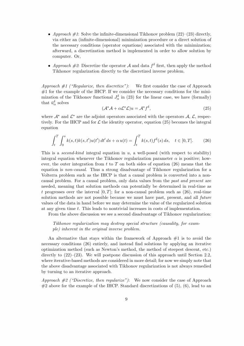
• Approach #1: Solve the infinite-dimensional Tikhonov problem (22)–(23) directly,via either an (infinite-dimensional) minimization procedure or a direct solution ofthe necessary conditions (operator equations) associated with the minimization;afterward, a discretization method is implemented in order to allow solution bycomputer. Or,

• Approach #2: Discretize the operator A and data f δ first, then apply the methodTikhonov regularization directly to the discretized inverse problem.

Approach #1 (“Regularize, then discretize”): We first consider the case of Approach#1 for the example of the IHCP. If we consider the necessary conditions for the mini-mization of the Tikhonov functional Jδ

α in (23) for the linear case, we have (formally)that uδ

α solves(A?A+ αL?L)u = A?f δ, (25)

where A? and L? are the adjoint operators associated with the operators A, L, respec-tively. For the IHCP and for L the identity operator, equation (25) becomes the integralequation∫ T

t

∫ s

0k(s, t)k(s, t′)u(t′) dt′ ds + α u(t) =

∫ T

tk(s, t)f δ(s) ds, t ∈ [0, T ]. (26)

This is a second-kind integral equation in u, a well-posed (with respect to stability)integral equation whenever the Tikhonov regularization parameter α is positive; how-ever, the outer integration from t to T on both sides of equation (26) means that theequation is non-causal. Thus a strong disadvantage of Tikhonov regularization for aVolterra problem such as the IHCP is that a causal problem is converted into a non-causal problem. For a causal problem, only data values from the past and present areneeded, meaning that solution methods can potentially be determined in real-time ast progresses over the interval [0, T ]; for a non-causal problem such as (26), real-timesolution methods are not possible because we must have past, present, and all futurevalues of the data in hand before we may determine the value of the regularized solutionat any given time t. This leads to nontrivial increases in costs of implementation.

From the above discussion we see a second disadvantage of Tikhonov regularization:

Tikhonov regularization may destroy special structure (causality, for exam-ple) inherent in the original inverse problem.

An alternative that stays within the framework of Approach #1 is to avoid thenecessary conditions (26) entirely, and instead find solutions by applying an iterativeoptimization method (such as Newton’s method, the method of steepest descent, etc.)directly to (22)–(23). We will postpone discussion of this approach until Section 2.2,where iterative-based methods are considered in more detail; for now we simply note thatthe above disadvantage associated with Tikhonov regularization is not always remediedby turning to an iterative approach.

Approach #2 (“Discretize, then regularize”): We now consider the case of Approach#2 above for the example of the IHCP. Standard discretizations of (5), (6), lead to an

9

equation of the form (7), where we recall that the N ×N matrix A is lower-triangular.If we now apply Tikhonov regularization directly to the discrete system (7), we solvethe finite-dimensional minimization problem

minu∈RN

‖Au− f δ‖2 + α‖u‖2

where we have again used the identity for the regularization operator, and where ‖ · ‖denotes the usual Euclidean norm. Now taking the approach of solving the necessaryconditions associated with the minimization problem, these conditions reduce to thematrix equation for the discrete Tikhonov solution uN,δ

α ,

(ATA + α I)u = AT f δ, (27)

where I is the N × N identity matrix. Even when we “discretize before regularizing”,we see evidence of how Tikhonov regularization may destroy special structure in prob-lems. The matrix A in the discrete IHCP (7) is lower-triangular allowing for sequentialsolution techniques, while the governing matrix (ATA + α I) in (27) is a full matrixrequiring far more expensive solution techniques.

We now turn to a second common form of regularization for inverse problems,namely, iterative regularization.

2.2 Iterative regularization.

Tikhonov regularization may not always be an attractive alternative for nonlinearinverse problems. One of the difficulties in the nonlinear case is that the functional Jδ

α in(23) is no longer strictly convex (in contrast to the linear case), leading to the possibilityof multiple local minima. In addition, it is generally not computationally feasible tofind any of the minima of (23) in the nonlinear case (see [20, 25] and the referencestherein). These difficulties make an alternative class of regularization methods, iterativeregularization methods, extremely attractive for nonlinear problems. We should mentionthat iterative regularization methods can also be very competitive methods for linearinverse problems.

In iterative regularization, one picks an initial guess u0 (a function, if we have notyet discretized the inverse problem) for the unknown solution u, and then one iterativelyconstructs updated approximations via a scheme like

un+1 = Un(un; f δ), n = 0, 1, . . . ,

where f δ is the usual measured data and Un is determined by the particular iterativeprocess. For even the best iterative methods one does not want to let the iterationparameter n to get too large because this may cause the noise in f δ to be amplifiedto the point where the results are no longer reliable. The regularization parameterassociated with iterative regularization is thus the (f δ, δ)-dependent stopping point ofthe iterative sequence, and an important part of the mathematical theory is in thedevelopment of stopping criteria for terminating the iteration. (Alternatively, one mayimplement regularization via a coordination of the iterative scheme with some other

10

form of regularization, such as the process of applying a gradient-like iterative proceduredirectly to the minimization of a Tikhonov functional.)

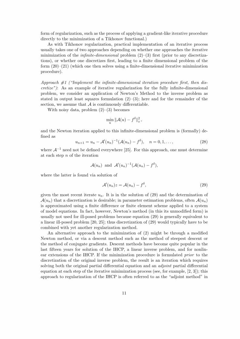
As with Tikhonov regularization, practical implementation of an iterative processusually takes one of two approaches depending on whether one approaches the iterativeminimization of the infinite-dimensional problem (2)–(3) first (prior to any discretiza-tions), or whether one discretizes first, leading to a finite dimensional problem of theform (20)–(21) (which one then solves using a finite-dimensional iterative minimizationprocedure).

Approach #1 (“Implement the infinite-dimensional iteration procedure first, then dis-cretize”): As an example of iterative regularization for the fully infinite-dimensionalproblem, we consider an application of Newton’s Method to the inverse problem asstated in output least squares formulation (2)–(3); here and for the remainder of thesection, we assume that A is continuously differentiable.

With noisy data, problem (2)–(3) becomes

minu‖A(u)− f δ‖2

Y,

and the Newton iteration applied to this infinite-dimensional problem is (formally) de-fined as

un+1 = un −A′(un)−1(A(un)− f δ), n = 0, 1, . . . , (28)

where A−1 need not be defined everywhere [25]. For this approach, one must determineat each step n of the iteration

A(un) and A′(un)−1(A(un)− f δ),

where the latter is found via solution of

A′(un)z = A(un)− f δ, (29)

given the most recent iterate un. It is in the solution of (29) and the determination ofA(un) that a discretization is desirable; in parameter estimation problems, often A(un)is approximated using a finite difference or finite element scheme applied to a systemof model equations. In fact, however, Newton’s method (in this its unmodified form) isusually not used for ill-posed problems because equation (29) is generally equivalent toa linear ill-posed problem [20, 25]; thus discretization of (29) would typically have to becombined with yet another regularization method.

An alternative approach to the minimization of (2) might be through a modifiedNewton method, or via a descent method such as the method of steepest descent orthe method of conjugate gradients. Descent methods have become quite popular in thelast fifteen years for solution of the IHCP, a linear inverse problem, and for nonlin-ear extensions of the IHCP. If the minimization procedure is formulated prior to thediscretization of the original inverse problem, the result is an iteration which requiressolving both the original partial differential equation and an adjoint partial differentialequation at each step of the iterative minimization process (see, for example, [2, 3]); thisapproach to regularization of the IHCP is often referred to as the “adjoint method” in

11

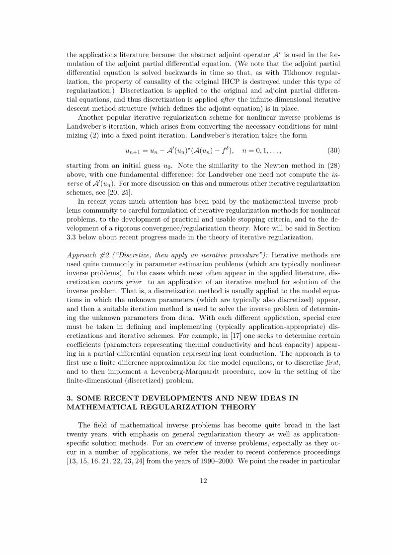
the applications literature because the abstract adjoint operator A? is used in the for-mulation of the adjoint partial differential equation. (We note that the adjoint partialdifferential equation is solved backwards in time so that, as with Tikhonov regular-ization, the property of causality of the original IHCP is destroyed under this type ofregularization.) Discretization is applied to the original and adjoint partial differen-tial equations, and thus discretization is applied after the infinite-dimensional iterativedescent method structure (which defines the adjoint equation) is in place.

Another popular iterative regularization scheme for nonlinear inverse problems isLandweber’s iteration, which arises from converting the necessary conditions for mini-mizing (2) into a fixed point iteration. Landweber’s iteration takes the form

un+1 = un −A′(un)?(A(un)− f δ), n = 0, 1, . . . , (30)

starting from an initial guess u0. Note the similarity to the Newton method in (28)above, with one fundamental difference: for Landweber one need not compute the in-verse of A′(un). For more discussion on this and numerous other iterative regularizationschemes, see [20, 25].

In recent years much attention has been paid by the mathematical inverse prob-lems community to careful formulation of iterative regularization methods for nonlinearproblems, to the development of practical and usable stopping criteria, and to the de-velopment of a rigorous convergence/regularization theory. More will be said in Section3.3 below about recent progress made in the theory of iterative regularization.

Approach #2 (“Discretize, then apply an iterative procedure”): Iterative methods areused quite commonly in parameter estimation problems (which are typically nonlinearinverse problems). In the cases which most often appear in the applied literature, dis-cretization occurs prior to an application of an iterative method for solution of theinverse problem. That is, a discretization method is usually applied to the model equa-tions in which the unknown parameters (which are typically also discretized) appear,and then a suitable iteration method is used to solve the inverse problem of determin-ing the unknown parameters from data. With each different application, special caremust be taken in defining and implementing (typically application-appropriate) dis-cretizations and iterative schemes. For example, in [17] one seeks to determine certaincoefficients (parameters representing thermal conductivity and heat capacity) appear-ing in a partial differential equation representing heat conduction. The approach is tofirst use a finite difference approximation for the model equations, or to discretize first,and to then implement a Levenberg-Marquardt procedure, now in the setting of thefinite-dimensional (discretized) problem.

3. SOME RECENT DEVELOPMENTS AND NEW IDEAS INMATHEMATICAL REGULARIZATION THEORY

The field of mathematical inverse problems has become quite broad in the lasttwenty years, with emphasis on general regularization theory as well as application-specific solution methods. For an overview of inverse problems, especially as they oc-cur in a number of applications, we refer the reader to recent conference proceedings[13, 15, 16, 21, 22, 23, 24] from the years of 1990–2000. We point the reader in particular

12

to the excellent volume [15] (which appeared in the year 2000) containing surveys ofnumerous types of solution methods for inverse problems. Each paper in that referencewas selected, according to the editors, because it typified “a new or promising methodthat could have impact on a wide variety of inverse problems” [15].

Below we highlight three areas of new development in the area of mathematical reg-ularization theory for inverse problems.

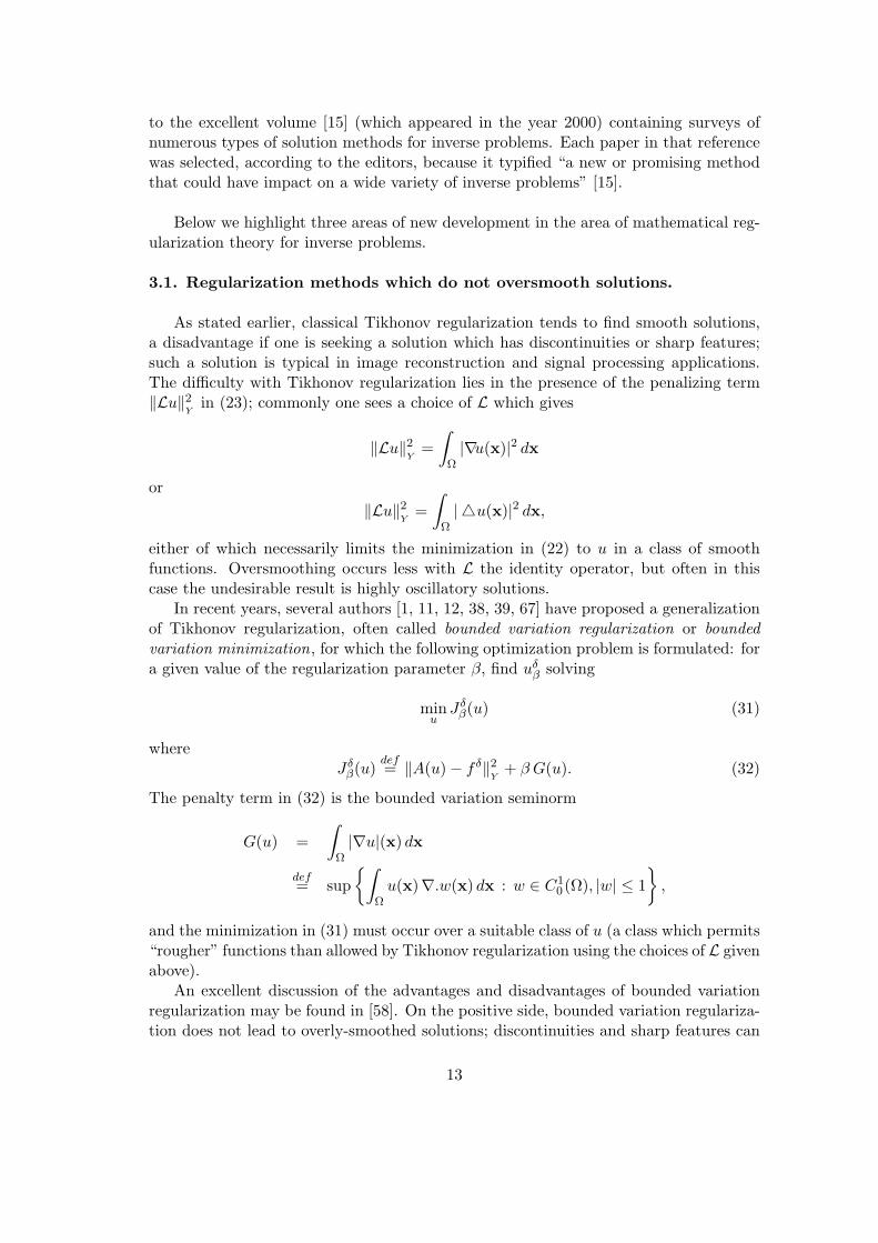
3.1. Regularization methods which do not oversmooth solutions.

As stated earlier, classical Tikhonov regularization tends to find smooth solutions,a disadvantage if one is seeking a solution which has discontinuities or sharp features;such a solution is typical in image reconstruction and signal processing applications.The difficulty with Tikhonov regularization lies in the presence of the penalizing term‖Lu‖2

Yin (23); commonly one sees a choice of L which gives

‖Lu‖2Y

=∫

Ω|∇u(x)|2 dx

or‖Lu‖2

Y=

∫Ω| 4u(x)|2 dx,

either of which necessarily limits the minimization in (22) to u in a class of smoothfunctions. Oversmoothing occurs less with L the identity operator, but often in thiscase the undesirable result is highly oscillatory solutions.

In recent years, several authors [1, 11, 12, 38, 39, 67] have proposed a generalizationof Tikhonov regularization, often called bounded variation regularization or boundedvariation minimization, for which the following optimization problem is formulated: fora given value of the regularization parameter β, find uδ

β solving

minu

Jδβ(u) (31)

whereJδ

β(u)def= ‖A(u)− f δ‖2

Y+ β G(u). (32)

The penalty term in (32) is the bounded variation seminorm

G(u) =∫

Ω|∇u|(x) dx

def= sup

∫Ω

u(x)∇.w(x) dx : w ∈ C10 (Ω), |w| ≤ 1

,

and the minimization in (31) must occur over a suitable class of u (a class which permits“rougher” functions than allowed by Tikhonov regularization using the choices of L givenabove).

An excellent discussion of the advantages and disadvantages of bounded variationregularization may be found in [58]. On the positive side, bounded variation regulariza-tion does not lead to overly-smoothed solutions; discontinuities and sharp features can

13

be captured by the process. Two disadvantages are that the regularization does not sta-bilize the problem in the bounded variation norm, and (of great importance to practicalimplementation) the penalty term in Jδ

β is not differentiable. The latter problem leadsto nontrivial difficulties in that one may not use standard (differentiable) optimizationpackages to solve the minimization problem; as a result, numerical implementation iscostly and slow speed of convergence is a factor. Thus, although the recent idea ofbounded variation regularization appears to be an attractive way to solve inverse prob-lems when solutions are not smooth, the method comes equipped with some distinctdisadvantages that must be handled in some manner.

To obtain the same success in capturing sharp features of solutions as bounded vari-ation regularization without some of the down sides of that method, different strategieshave taken (for example) by Coleman, Dobson, Li, Liu, Santosa, and others, to dealdirectly with the nondifferentiable cost functional, applying either an affine scaling ap-proach or a quadratic programming strategy (see the references in [19]). A differentpoint of view has been taken by Vogel, Dobson, Oman, and others, in which Jδ

β in (32)is altered slightly in order to restore differentiability of the cost functional and thus toallow for implementation of effective differentiable computational methods (see, e.g.,[1]). An improvement (which also unifies some of the previous ideas) has been found re-cently in [58]. We do not detail the formulation of this approach here because it is quitetechnical; nevertheless the results seem to be applicable to many problems of interestin applications.

We note that an alternative approach to the problem of finding “rough” solutions ofinverse problems may also be found in some of the local regularization methods givenin Section 3.2 below. These approaches take a more classical formulation, via classicalTikhonov regularization, but they allow the use of a variable Tikhonov regularizationparameter. That is, instead of using α a constant in (22)–(23), these methods allow forα to vary with the spatial location x, as x ranges over the domain Ω of the solution.This approach allows for more regularization (i.e., smoothness) in some regions of thesolution and less regularization (i.e., roughness) in others. This certainly allows for oneto find some sharp features of solutions, but does not presently allow for the recoveryof discontinuities.

3.2. Localized regularization methods.

Another new development in the mathematical theory of regularization is that oflocalized regularization methods which have been primarily studied for linear inverseproblems. The advantages of such methods are generally that special structures of theoriginal inverse problem can often be preserved, leading to savings in implementationand computational costs. For example, while Tikhonov regularization destroys thecausal nature of Volterra problems such as the IHCP (as discussed above), the localregularization methods developed in [14, 42, 44, 45, 46, 48, 49, 52, 53] do not havethis problem. Local regularization of equation (1) is based on a decomposition of theoperator A and the data f into “local” and “nonlocal” parts. Then regularization isapplied to problem of inverting the local part of A only. Because space is limited, wewill present only a brief idea of local regularization methods here; in particular, we willfocus mainly on local regularization methods for a Volterra inverse problem such as the

14

IHCP.We recall that the “true” solution u of the IHCP solves an equation of the form∫ t

0k(t, s)u(s) ds = f(t), t ∈ [0, T ]. (33)

To motivate the ideas of local regularization, we let r > 0 be a small fixed constant andassume that equation (33) actually holds on an extended domain [0, T + r] (which canalways be accomplished by simply decreasing the size of T slightly). Then u satisfies∫ t+ρ

0k(t + ρ, s)u(s) ds = f(t + ρ), t ∈ [0, T ], ρ ∈ [0, r],

or, splitting the integral at t and making a change of integration variable,∫ t

0k(t + ρ, s)u(s) ds +

∫ ρ

0k(t + ρ, t + s)u(t + s) ds = f(t + ρ), t ∈ [0, T ], ρ ∈ [0, r].

For each t ∈ [0, T ], the ρ variable serves to advance the equation slightly into the future.One way to consolidate this future information is to integrate both sides of the equationwith respect to ρ, i.e.,∫ t

0

∫ r

0k(t+ρ, s) dρ u(s) ds +

∫ r

0

∫ ρ

0k(t+ρ, t+s)u(t+s) ds dρ (34)

=∫ r

0f(t + ρ) dρ, t ∈ [0, T ],

where we have made a change of order of integration in the first integral above. (It isworth remarking that a more general approach, not detailed here, is to integrate withrespect to a Borel measure η = η(ρ); this approach generates an entire class of localregularization methods [44].)

We note that the true solution u satisfies equation (34); when f is replaced byf δ, a regularized form of this equation is needed and we obtain this new equation byreplacing u(t + s) by u(t) in the second integral term. That is, for fixed t, it is as if uis (temporarily) assumed to be constant on the small local interval [t, t + r]; the lengthr of this local interval becomes the regularization parameter. The “local regularizationequation” which results is given by∫ t

0k(t, s; r)u(s) ds + a(t; r) u(t) = f δ(t; r), t ∈ [0, T ], (35)

where

a(t; r) :=∫ r

0

∫ ρ

0k(t + ρ, t + s) ds dρ, (36)

k(t, s; r) :=∫ r

0k(t + ρ, s) dρ, (37)

f δ(t; r) :=∫ r

0f δ(t + ρ) dρ. (38)

15

We may regularize further by adding penalty term to (35), i.e.,∫ t

0k(t, s; r)u(s) ds + [a(t; r) + α(t)]u(t) = f δ(t; r), t ∈ [0, T ], (39)

where α = α(t) is a nonnegative penalty function. The t-dependence of α allows forvariable regularization, that is, more regularization at some locations t in the domain[0, T ] and less at other locations. See [52, 53] for more discussion on this additional regu-larization parameter and for some numerical examples involving variable regularizationparameters.

A regularization theory for this method was developed in [44] (for convolution ker-nels) and [52] (for nonconvolution kernels) provided that the kernel k satisfies k ∈ C1

with k(t, t) 6= 0 for t ∈ [0, T + r]. Under these conditions, a choice of the regularizationparameter r = r(δ) may be made which guarantees r(δ) → 0, and

uδ(·; r(δ)) → u as δ → 0, (40)

where uδ solves equation (35) for the given value of r(δ). In the case of equation (39),a similar statement about convergence of the solution of that equation may be made,for a choice of r = r(δ) and α = α(t, δ).

Further convergence results (for more general kernels k) may be found in [14, 42,44, 45, 46, 48, 49, 52, 53]; convergence results for discretizations of (35) and (39) maybe found in [42] and [53]. We note also that a special case of this local regularizationmethod has been successfully used in a number of practical applications, including over30 years of use by practitioners solving the IHCP [8]. In the applications, this methodis often known as “Beck’s method” and is named after its developer, J. V. Beck. Wenote that the IHCP is a particularly difficult Volterra example from the standpoint ofill-posedness, and that none of the existing convergence theory on local regularizationapplies to the IHCP.

For the above example, the ideas of local regularization are used to transform an ill-posed first-kind Volterra equation into a well-posed second-kind Volterra equation, muchlike Tikhonov regularization was shown to do for the IHCP. In contrast to Tikhonov reg-ularization, which requires all future values of the data in order to be able to constructan approximate solution at time t (i.e., the Tikhonov equation is very non-causal), thelocal regularization method only uses a very small amount of future information foreach t. This means that implementation has the potential to be carried out in “nearreal-time”. In fact, it can be shown that discretization of equations associated withTikhonov regularization takes O(N3) multiplies, while the local regularization methodtakes only O(1

2N2) multiplies, a considerable savings in cost; both estimates of cost arefor the general nonconvolution Volterra problem [47].

Local regularization can also be extended to problems like the image reconstructionproblem. In this case the operator A is not of Volterra type and an alternate localapproach (the description of which is too long for this paper) is used. In the non-Volterra case, an iterative solution method must be combined with the method of localregularization; if the number of iterations is small, then local regularization of non-Volterra problems can be a savings over standard Tikhonov regularization for suchproblems [47].

16

As stated earlier, another feature of local regularization is the capability for allowingvariable regularization parameters. We have already seen how the additional regular-ization parameter α can vary with respect to the independent variable. In addition, theparameter r above could be variable instead of a fixed constant, allowing for more orless regularization at a given location in the domain. See [48, 52, 53] for a theory basedon the use of variable regularization parameters, and for examples which illustrate howa regularization parameter may be selected using a variable discrepancy principle.

There remain a number of open questions and problems associated with the theoryof local regularization. For the Volterra problem, there is a serious limitation on thetypes of kernels k for which a mathematical convergence/regularization theory may beproven. As indicated earlier, the kernel k associated with the IHCP does not fall withinthe class of such kernels. Numerical evidence in [60] indicates that stability may notin fact be present for a certain class of kernels, although lack of stability has not beenactually proven. It is evident that more work is needed to modify local regularizationmethods so that a mathematical convergence/regularization theory may be developedfor a large class of kernels k.

Another open problem concerns the development of a theory (perhaps involvinga classical discrepancy principle) for the selection of local regularization parameters rand α. Although numerical examples exist for selection of such variable regularizationparameters [52, 53] no theoretical results are available at the present time.

Finally, we note that the local regularization method presented here is by no meansthe only possibility for a localized regularization approach. For example, we mentionthe theory of mollification (see, e.g., [54, 55, 56, 57] and see [41] for shortcomings of thisapproach for general Volterra problems), and also the work on distributional approxi-mations of Nashed and Scherzer in [58].

3.3. Progress on iterative regularizations methods for nonlinear inverseproblems.

As indicated above, iterative methods for the solution of nonlinear inverse problemsare typically in the form of

un+1 = Un(un; f), n = 0, 1, . . . , (41)

in the case where one has “ideal” data f , and in the case of perturbed data f δ (where‖f − f δ‖Y ≤ δ for some δ > 0), we have the iteration

uδn+1 = Un(uδ

n; f δ), n = 0, 1, . . . .

In both cases above, an initial guess u0 must be supplied by the user, while Un isprovided by the particular iterative method and depends in large part on A and itsproperties. For a given iterative procedure, the mathematical theory of this iteration asa regularization method for an inverse problem usually entails the following:

(a) Determination of conditions on the operator A which guarantee convergence ofun to u in the case where “ideal” data f is used in the iterative process;

17

(b) Definition of a stopping criteria for the iteration in the case of perturbed data f δ;that is, given δ and f δ, we only iterate for n = 0, 1, . . . n, where n = n(δ, f δ). Forthis selection of n, the mathematical theory should show that n(δ, f δ) →∞ and

uδn(δ,fδ) → u (42)

as δ → 0, i.e., that the iteration method with stopping criteria is a regularizationmethod; and

(c) Determination of conditions on the operator A for which a convergence rate maybe given for the convergence in (42).

In the excellent survey [25], Engl and Scherzer detail the progress made in (a)–(c)above for a number of important iteration methods which are of great practical usein nonlinear inverse problems appearing widely in applications. In particular, muchdevelopment in the last few years has taken place in advancing the theory of Landweberiteration for nonlinear inverse problems. Convergence of the Landweber iteration wasshown in [62] using the fact that the operator Un for Landweber iteration can be writtenindependent of n, i.e., Un = U , where for ideal data,

U(u) = u−A′(u)?(A(u)− f).

This means that the iteration in (41) can be viewed as a fixed point iteration, for whichfixed point theory may be used to derive weak convergence of the iteration dependingon assumptions on U . In [31], a convergence theory was developed which makes use ofstructure of the operator A (rather than U); in fact, proofs of (a)–(c) may be found inthat reference, with the stopping criteria in (b) developed using a discrepancy principle.The iteration is to be stopped after n steps where n = n(δ, f δ) satisfies the following

‖A(uδn)− f δ‖ ≤ τδ < ‖A(uδ

n)− f δ‖, 0 ≤ n < n,

for τ a positive number depending on the properties of A [25, 31]. The convergencerate (in (c)) found in [31] requires conditions on A which are generally too restrictivefor strongly smoothing operators; alternative convergence rate results (for more generaloperators) may be found in [18].

A theory for the iterative method of steepest descent and the method of minimalerror (see [25]) has also been developed for nonlinear inverse problems. In [59, 61], parts(a) and (b) were proven, while in [59], convergence rates in (c) were proven.

We have limited our discussion here to progress made on the Landweber, steepestdescent, and minimal error iterations. For a more complete discussion of these methods,and for progress made in the mathematical analysis of other iterations, such as Newton’sMethod, Modified and Inexact Newton Methods (Levenberg-Marquardt, Gauss-Newton,etc.), the reader is referred to [25].

One of the present shortcomings of the theory for iterative regularization is that con-ditions on A needed to prove (a)–(c) are difficult to verify in practice. These conditionshave been analyzed for some particular applications [20, 25]. For example, one may findan analysis of certain assumptions needed for the Landweber theory in [30, 32, 35, 36, 37](for inverse scattering problems), in [33] (for inverse potential problems), in [9, 31] (for

18

parameter estimation in ordinary differential equations), in [40] (for parameter estima-tion in a hyperbolic partial differential equation), and in [34] (for the determination ofa discontinuity in a conductivity in an elliptic equation), to name a few applications.Because of the importance of having precise statements of convergence such as (a)–(c)in every instance in which an iteration is applied, it is clear that more work is neededon the development of assumptions on A which may be proven for a wider set of appli-cations, and for a larger class of iterative schemes that are commonly in use.

4. CONCLUSION

In this paper we have reviewed some of the new developments in the theory of mathe-matical regularization for inverse problems, indicating briefly where some of this theorycurrently falls short. Numerous open problems in these and other theoretical areasmean that there will be an rich source of research problems in the area of mathematicalregularization theory for many years to come.

References

[1] Acar, R., and Vogel, C. R., 1994, Analysis of bounded variation penalty methodsfor ill-posed problems, Inverse Problems, Vol 10, pp 1217–1229.

[2] Alifanov, O. M., 1994, Inverse Heat Transfer Problems, Spring-Verlag, Berlin.

[3] Alifanov, O. M., Artyukhin, E. A., and Rumyantsev, S. V., 1988, Extreme methodsof solving ill-posed problems, Nauka, Moscow.

[4] Banks, H. T., Kareiva, P., and Lamm, P., 1985, Estimation techniques for transportequations, Springer Lecture Notes in Biomathematics (Capasso, V., et al, editors),vol. 57, Springer, New York, pp 428–438.

[5] Banks, H. T., Kareiva, P., and Lamm, P. K., 1985, Modeling insect dispersal and es-timating parameters when mark-release techniques may cause initial disturbances,J. Math. Biology, Vol 22, pp 259–277.

[6] Banks, H. T., and Kunisch, K., 1989, Estimation Techniques for Distributed Pa-rameter Systems, Birkhauser, Boston.

[7] Banks, H. T, Lamm, P. K., and Armstrong, E. S., 1986, Spline-based distributedsystem identification with application to large space antennas, AIAA J. GuidanceControl and Dynamics, Vol 9, pp 304–311.

[8] Beck, J. V., Blackwell, B., and St. Clair, Jr., C. R., 1985, Inverse heat conduction,Wiley-Interscience, New York.

[9] Binder, A., Hanke, M., and Scherzer, O., 1996, On the Landweber iteration fornonlinear ill-posed problems, J. Inverse Ill-Posed Problems, Vol 4, pp 381–389.

[10] Cannon, J. R., 1984, The One-Dimensional Heat Equation, in The Encyclopediaof Mathematics and its Applications, Volume 23, Addison-Wesley, Reading, MA.

19

[11] Chambolle, A., and Lions, P.-L., 1997, Image recovery via total variation mini-mization and related problems, Numer. Math., Vol 76, pp 167–188.

[12] Chavent, G., and Kunisch, K., 1997, Regularization of linear least squares prob-lems by total bounded variation, ESAIM: Control, Optimisation, and Calculus ofVariations, Vol 2, pp 359–376.

[13] Chavent, G., and Sabatier, P. C. (editors), 1997, Inverse Problems of Wave Prop-agation and Diffraction, Springer, Berlin.

[14] Cinzori, A. C., and Lamm, P. K., 2000, Future polynomial regularization of first-kind Volterra operators, SIAM J. Num. Anal., Vol 37, pp 949–979.

[15] Colton, D., Engl, H. W., Louis, A. K., McLaughlin, J. R., and Rundell, W. (ed-itors), 2000, Surveys on Solution Methods for Inverse Problems, Springer, Wien,New York.

[16] Colton, D., Ewing, R., and Rundell, W. (editors), 1990, Inverse Problems in PartialDifferential Equations, SIAM, Philadelphia.

[17] De Carvalho, G., Silva Neto, A. J., 1999, An inverse analysis for polymers thermalproperties estimation, Proc. 3rd International Conference on Inverse Problems inEngineering: Theory and Practice, Port Ludlow, WA, USA.

[18] Deuflhard, P., Engl, H. W., and Scherzer, O., 1998, A convergence analysis ofiterative methods for the solution of nonlinear ill-posed problems under affinelyinvariant conditions, Inverse Problems, Vol 14, pp 1081–1106.

[19] Dobson, D. C., and Santosa, F., 1996, Recovery of blocky images from noisy andblurred data, SIAM J. Applied Math., Vol 56, pp 1181–1198.

[20] Engl, H. W., Hanke, M., and Neubauer, A., 1996, Regularization of inverse prob-lems, Kluwer Academic Publishers Group, Dordrecht.

[21] Engl, H. W., Louis, A. K., and Rundell, W. (editors), 1996, Inverse Problems inGeophysical Applications, SIAM, Philadelphia.

[22] Engl, H. W., Louis, A. K., and Rundell, W. (editors), 1996, Inverse Problems inMedical Imaging and Nondestructive Testing, Springer, Wien, New York.

[23] Engl, H. W., and McLaughlin, J. R. (editors), 1994, Inverse Problems and OptimalDesign in Industry, B. G. Teubner, Stuttgart.

[24] Engl, H. W., and Rundell, W. (editors), 1995, Inverse Problems in Diffusion Pro-cesses, SIAM, Philadelphia.

[25] Engl, H. W., and Scherzer, O., 2000, Convergence rates results for iterative methodsfor solving nonlinear ill-posed problems, Surveys on Solution Methods for InverseProblems (Colton, et al, editors), Springer, Vienna, pp 1–34.

[26] Gripenberg, G., Londen, S.-O., and Staffans, O., 1990, Volterra integral and func-tional equations, Cambridge University Press, Cambridge-New York.

20

[27] Groetsch, C. W., 1993, Inverse Problems in the Mathematical Sciences, Vieweg,Wiesbaden.

[28] Groetsch, C. W., 1984, The Theory of Tikhonov Regularization for Fredholm Equa-tions of the First Kind, Pitman, Boston.

[29] Hanke, M. , 2000, Iterative Regularization Techniques in Image Reconstruction,Surveys on Solution Methods for Inverse Problems, (Colton, D., et al, editors),Springer, Vienna, pp 35–52.

[30] Hanke, M., Hettlich, F., and Scherzer, O., 1995, The Landweber iteration for aninverse scattering problem, Proceedings of the 1995 Design Engineering TechnicalConferences (Wang, et al, editors), Vibration Control, Analysis, and Identification,Vol 3, Part C, ASME, New York, pp 909–915.

[31] Hanke, M., Neubauer, A., Scherzer, O., 1995, A convergence analysis of Landweberiteration for nonlinear ill-posed problems, Numer. Math., Vol 72, pp 21–37.

[32] Hettlich, F., 1996, An iterative method for the inverse scattering problem fromsound-hard obstacles, Z. Angew. Math. Mech., Vol 76, pp 165–168.

[33] Hettlich, F., and Rundell, W., 1996, Iterative methods for the reconstruction of aninverse potential problem, Inverse Problems, Vol 12, pp 251–266.

[34] Hettlich, F., and Rundell, W., 1998, The determination of a discontinuity in aconductivity from a single boundary measurement, Inverse Problems, Vol 14, pp67–82.

[35] Hohage, T., 1999, Convergence rates of a regularized Newton method in sound-hardinverse scattering, SIAM J. Numer. Analysis, Vol 36, pp 125-142.

[36] Hohage, T., 1997, Logarithmic convergence rates of the iteratively regularizedGauss-Newton method for an inverse potential and an inverse scattering problem,Inverse Problems, Vol 13, pp 1279–1300.

[37] Hohage, T., and Schormann, C., 1998, A Newton-type method for a transmissionproblem in inverse scattering, Inverse Problems, Vol 14, pp 1207–1228.

[38] Ito, K., and Kunisch, K., An active set strategy based on the augmented Lagrangianformulation for image restoration, preprint.

[39] Ito, K., and Kunisch, K., Augmented Lagrangian methods for nonsmooth convexoptimization in Hilbert spaces, preprint.

[40] Kabanikhin, S., Kowar, R., and Scherzer, O., 1998, On the Landweber iteration forthe solution of a parameter identification problem in a hyperbolic partial differentialequation of second order, J. Inv. Ill-Posed Problems, Vol 6, pp 403–430.

[41] Lamm, P. K., 2000, A survey of regularization methods for first-kind Volterraequations, Surveys on Solution Methods for Inverse Problems, (Colton, D., et al,editors), Springer, Vienna, pp 53–82.

21

[42] Lamm, P. K., 1996, Approximation of ill-posed Volterra problems via predictor-corrector regularization methods, SIAM J. Applied Math., Vol 56, pp 524– 541.

[43] Lamm, P. K., 1987, Estimation of discontinuous coefficients in parabolic systems:applications to reservoir simulation, SIAM J. Control and Optimization, Vol 25,pp 18–37.

[44] Lamm, P. K., 1995, Future-sequential regularization methods for ill-posed Volterraequations. Applications to the inverse heat conduction problem, J. Math. Anal.Appl., Vol 195, No. 2, pp 469–494.

[45] Lamm, P. K., 1995, On the Local Regularization of Inverse Problems of VolterraType, Proceedings of the 1995 Design Engineering Technical Conferences (Wang, etal, editors), Vibration Control, Analysis, and Identification, Vol 3, Part C, ASME,New York.

[46] Lamm, P. K., 1997, Regularized inversion of finitely smoothing Volterra operators:predictor-corrector regularization methods, Inverse Problems, Vol 13, pp 375 – 402.

[47] Lamm, P. K., 2001, Variable smoothing local regularization methods for first-kindintegral equations, preprint.

[48] Lamm, P. K., 1999, Variable-smoothing regularization methods for inverse prob-lems, Theory and Practice of Control and Systems (Tornambe, A., et al, editors),World Scientific.

[49] Lamm, P. K., and Elden, L., 1997, Numerical solution of first-kind Volterra equa-tions by sequential Tikhonov regularization, SIAM J. Numerical Anal., Vol 34, pp1432–1450.

[50] Lamm, P. K., and Murphy, K. A., 1988, Estimation of discontinuous coefficientsand boundary parameters for hyperbolic systems, Quarterly Appl. Math., Vol 46,pp 1–22.

[51] Lamm, P. K., and Rosen, I. G., 1991, An approximation theory for the estimationof parameters in degenerate Cauchy problems, J. Math. Analysis and Appl., Vol162, pp 13–48.

[52] Lamm, P. K., and Scofield, T. L, 2001, Local regularization methods for the stabi-lization of ill-posed Volterra problems, to appear in Numer. Funct. Anal. Opt..

[53] Lamm, P. K., and Scofield, T. L, 2000, Sequential predictor-corrector methods forthe variable regularization of Volterra inverse problems, Inverse Problems, Vol 16,pp 373–399.

[54] Louis, A. K., 1996, Approximate inverse for linear and some nonlinear problems,Inverse Problems, Vol 12, No 2, pp 175–190.

[55] Louis, A. K., 1997, Application of the approximate inverse to 3D X-ray CT andultrasound tomography, Inverse Problems in Medical Imaging and NondestructiveTesting (Oberwolfach, 1996) Springer, Vienna, pp. 120–133.

22

[56] Louis, A. K., 1999, A unified approach to regularization methods for linear ill-posedproblems, Inverse Problems, Vol 15, pp 489–498.

[57] Murio, D. A., 1993, The mollification method and the numerical solution of ill-posed problems, John Wiley & Sons, Inc., New York.

[58] Nashed, M. Z., and Scherzer, O., 1998, Least squares and bounded variation regu-larization with nondifferentiable functionals, Numer. Funct. Anal. Opt., Vol 19, pp873–901.

[59] Neubauer, A., and Scherzer, O., 1995, A convergence rate result for a steepestdescent method and a minimal error method for the solution of nonlinear ill-posedproblems, Z. Anal. Anwend., Vol 14, 369–377.

[60] Ring, W., and Prix, J., 2000, Sequential predictor–corrector regularization methodsand their limitations, Inverse Problems, Vol 16, No 3, pp 619–634.

[61] Scherzer, O., 1996, A convergence analysis of a method of steepest descent anda two-step algorithm for nonlinear ill-posed problems, Numer. Funct. Anal. Opti-mization, Vol 17, pp 197–214.

[62] Scherzer, O., 1995, Convergence criteria of iterative methods based on Landweberiteration for solving nonlinear problems, J. Math. Anal. Appl., Vol 194, pp 911–933.

[63] Tanana, V. P., 1997, Methods for Solution of Nonlinear Operator Equations, VSP,Utrecht.

[64] Tikhonov, A. N., and Arsenin, V. Y, (John, F., translation editor), 1977, Solutionsof Ill-Posed Problems, John Wiley & Sons, Washington, D.C..

[65] Tikhonov, A. N., Goncharsky, A., Stepanov, V., and Yagola, A., 1995, NumericalMethods for the Solution of Ill-Posed Problems, Kluwer, Dordrecht.

[66] Vasin, V. V., and Ageev, A. L. , 1995, Ill-Posed Problems with A-Priori Informa-tion, VSP, Utrecht.

[67] Vogel, C., and Oman, M., 1996, Iterative methods for total variation denoising,SIAM J. Sci. Computing, Vol 17, pp 227–238.

[68] Wing, G. W., 1991, A Primer on Integral Equations of the First Kind, SIAM,Philadelphia.

23