Stochastic E�ects;Application in Nuclear PhysicsOleg Mazonka

�Swierk, February 11, 2000

.

Stochastic E�ects; Application in Nuclear Physics(February 11, 2000)Stochastic e�ects in nuclear physics refer to the study of the dynamics of nuclearsystems evolving under stochastic equations of motion. In this dissertation werestrict our attention to classical scattering models. We begin with introduc-tion of the model of nuclear dynamics and deterministic equations of evolution.We apply a Langevin approach | an additional property of the model, whichre ects the statistical nature of low energy nuclear behaviour. We then concen-trate our attention on the problem of calculating tails of distribution functions,which actually is the problem of calculating probabilities of rare outcomes.Two general strategies are proposed. Results and discussions follow. Finallyin the appendix we consider stochastic e�ects in nonequilibrium systems. Afew exactly solvable models are presented. For one model we show explicitlythat stochastic behaviour in a microscopic description can lead to ordered col-lective e�ects on the macroscopic scale. Two others are solved to con�rm thepredictions of the uctuation theorem.

i

ii ContentsContentsI. Introduction : : : : : : : : : : : : : : : : : : : : : : : : : : : : : : : : : : : : : : : : : : : : : : : : : : : : : : : : : : : : : : : : : : : : : :11. Introductory concepts : : : : : : : : : : : : : : : : : : : : : : : : : : : : : : : : : : : : : : : : : : : : : : : : : : : : : : : 1Fluctuations in classical description of Heavy Ion dynamics : : : : : : : : : : : : : : : : : 1Fluctuation-dissipation theorem : : : : : : : : : : : : : : : : : : : : : : : : : : : : : : : : : : : : : : : : : : : : 3Probabilities of rare events : : : : : : : : : : : : : : : : : : : : : : : : : : : : : : : : : : : : : : : : : : : : : : : : : 32. Outline of chapters : : : : : : : : : : : : : : : : : : : : : : : : : : : : : : : : : : : : : : : : : : : : : : : : : : : : : : : : : : 3II. Model of nuclear dynamics : : : : : : : : : : : : : : : : : : : : : : : : : : : : : : : : : : : : : : : : : : : : : : : : : : : : : : :51. Introduction : : : : : : : : : : : : : : : : : : : : : : : : : : : : : : : : : : : : : : : : : : : : : : : : : : : : : : : : : : : : : : : : :52. Shape parameterization : : : : : : : : : : : : : : : : : : : : : : : : : : : : : : : : : : : : : : : : : : : : : : : : : : : : : :53. Kinetic and potential energies; shell corrections : : : : : : : : : : : : : : : : : : : : : : : : : : : : : : :7Kinetic energy : : : : : : : : : : : : : : : : : : : : : : : : : : : : : : : : : : : : : : : : : : : : : : : : : : : : : : : : : : : : : 7Potential energy : : : : : : : : : : : : : : : : : : : : : : : : : : : : : : : : : : : : : : : : : : : : : : : : : : : : : : : : : : : 8Shell e�ects : : : : : : : : : : : : : : : : : : : : : : : : : : : : : : : : : : : : : : : : : : : : : : : : : : : : : : : : : : : : : : : :94. Equations of motion : : : : : : : : : : : : : : : : : : : : : : : : : : : : : : : : : : : : : : : : : : : : : : : : : : : : : : : : 10Generic deterministic equation : : : : : : : : : : : : : : : : : : : : : : : : : : : : : : : : : : : : : : : : : : : : 10Dissipation : : : : : : : : : : : : : : : : : : : : : : : : : : : : : : : : : : : : : : : : : : : : : : : : : : : : : : : : : : : : : : : 115. Fluctuations : : : : : : : : : : : : : : : : : : : : : : : : : : : : : : : : : : : : : : : : : : : : : : : : : : : : : : : : : : : : : : : :12Fokker-Planck equation : : : : : : : : : : : : : : : : : : : : : : : : : : : : : : : : : : : : : : : : : : : : : : : : : : : 12Derivation of uctuating force : : : : : : : : : : : : : : : : : : : : : : : : : : : : : : : : : : : : : : : : : : : : :13Di�usion term for Fermi particles : : : : : : : : : : : : : : : : : : : : : : : : : : : : : : : : : : : : : : : : : 15Langevin approach : : : : : : : : : : : : : : : : : : : : : : : : : : : : : : : : : : : : : : : : : : : : : : : : : : : : : : : :16Implementation of the Langevin equation : : : : : : : : : : : : : : : : : : : : : : : : : : : : : : : : : :186. Additional topics : : : : : : : : : : : : : : : : : : : : : : : : : : : : : : : : : : : : : : : : : : : : : : : : : : : : : : : : : : : 19Exchange of particles : : : : : : : : : : : : : : : : : : : : : : : : : : : : : : : : : : : : : : : : : : : : : : : : : : : : : 19Dissipative uctuations : : : : : : : : : : : : : : : : : : : : : : : : : : : : : : : : : : : : : : : : : : : : : : : : : : : 20Parameterization of the potential : : : : : : : : : : : : : : : : : : : : : : : : : : : : : : : : : : : : : : : : : :20III. Computation of small probabilities : : : : : : : : : : : : : : : : : : : : : : : : : : : : : : : : : : : : : : : : : : : : :241. Introduction : : : : : : : : : : : : : : : : : : : : : : : : : : : : : : : : : : : : : : : : : : : : : : : : : : : : : : : : : : : : : : : :24The probability : : : : : : : : : : : : : : : : : : : : : : : : : : : : : : : : : : : : : : : : : : : : : : : : : : : : : : : : : : :242. Polymer method : : : : : : : : : : : : : : : : : : : : : : : : : : : : : : : : : : : : : : : : : : : : : : : : : : : : : : : : : : : :25Polymer analogy : : : : : : : : : : : : : : : : : : : : : : : : : : : : : : : : : : : : : : : : : : : : : : : : : : : : : : : : : :25Action : : : : : : : : : : : : : : : : : : : : : : : : : : : : : : : : : : : : : : : : : : : : : : : : : : : : : : : : : : : : : : : : : : : :25Metropolis sweeps : : : : : : : : : : : : : : : : : : : : : : : : : : : : : : : : : : : : : : : : : : : : : : : : : : : : : : : : 25Computation of work : : : : : : : : : : : : : : : : : : : : : : : : : : : : : : : : : : : : : : : : : : : : : : : : : : : : : 26Advantages and disadvantages of the polymer method : : : : : : : : : : : : : : : : : : : : : 273. Examples : : : : : : : : : : : : : : : : : : : : : : : : : : : : : : : : : : : : : : : : : : : : : : : : : : : : : : : : : : : : : : : : : : 28Analytically solvable model : : : : : : : : : : : : : : : : : : : : : : : : : : : : : : : : : : : : : : : : : : : : : : : 28

Contents iiiSimpli�ed model of HIC : : : : : : : : : : : : : : : : : : : : : : : : : : : : : : : : : : : : : : : : : : : : : : : : : : 304. Importance Sampling Method : : : : : : : : : : : : : : : : : : : : : : : : : : : : : : : : : : : : : : : : : : : : : : :32Langevin dynamics : : : : : : : : : : : : : : : : : : : : : : : : : : : : : : : : : : : : : : : : : : : : : : : : : : : : : : : 33Importance sampling : : : : : : : : : : : : : : : : : : : : : : : : : : : : : : : : : : : : : : : : : : : : : : : : : : : : : 34Biasing Langevin trajectories : : : : : : : : : : : : : : : : : : : : : : : : : : : : : : : : : : : : : : : : : : : : : :35Langevin action : : : : : : : : : : : : : : : : : : : : : : : : : : : : : : : : : : : : : : : : : : : : : : : : : : : : : : : : : : 35Compensation for modi�cations : : : : : : : : : : : : : : : : : : : : : : : : : : : : : : : : : : : : : : : : : : : 37E�ciency gain : : : : : : : : : : : : : : : : : : : : : : : : : : : : : : : : : : : : : : : : : : : : : : : : : : : : : : : : : : : : 375. Application of ISM: practical matters : : : : : : : : : : : : : : : : : : : : : : : : : : : : : : : : : : : : : : : 39Calculating weights : : : : : : : : : : : : : : : : : : : : : : : : : : : : : : : : : : : : : : : : : : : : : : : : : : : : : : : 39Cut-o� : : : : : : : : : : : : : : : : : : : : : : : : : : : : : : : : : : : : : : : : : : : : : : : : : : : : : : : : : : : : : : : : : : : 40D depending on x : : : : : : : : : : : : : : : : : : : : : : : : : : : : : : : : : : : : : : : : : : : : : : : : : : : : : : : : 40Multidimensionality : : : : : : : : : : : : : : : : : : : : : : : : : : : : : : : : : : : : : : : : : : : : : : : : : : : : : : :40Inertial motion : : : : : : : : : : : : : : : : : : : : : : : : : : : : : : : : : : : : : : : : : : : : : : : : : : : : : : : : : : : 41Dissipative motion : : : : : : : : : : : : : : : : : : : : : : : : : : : : : : : : : : : : : : : : : : : : : : : : : : : : : : : : 42Elimination of degenerate directions : : : : : : : : : : : : : : : : : : : : : : : : : : : : : : : : : : : : : : :42Extension to the non-Marcovian case : : : : : : : : : : : : : : : : : : : : : : : : : : : : : : : : : : : : : :436. Examples : : : : : : : : : : : : : : : : : : : : : : : : : : : : : : : : : : : : : : : : : : : : : : : : : : : : : : : : : : : : : : : : : : 44Schematic model : : : : : : : : : : : : : : : : : : : : : : : : : : : : : : : : : : : : : : : : : : : : : : : : : : : : : : : : : :44Exactly solvable model : : : : : : : : : : : : : : : : : : : : : : : : : : : : : : : : : : : : : : : : : : : : : : : : : : : :46IV. Calculations : : : : : : : : : : : : : : : : : : : : : : : : : : : : : : : : : : : : : : : : : : : : : : : : : : : : : : : : : : : : : : : : : : :49Introduction : : : : : : : : : : : : : : : : : : : : : : : : : : : : : : : : : : : : : : : : : : : : : : : : : : : : : : : : : : : : : : : : : : 49Units and constants : : : : : : : : : : : : : : : : : : : : : : : : : : : : : : : : : : : : : : : : : : : : : : : : : : : : : : :491. Fusion probabilities : : : : : : : : : : : : : : : : : : : : : : : : : : : : : : : : : : : : : : : : : : : : : : : : : : : : : : : : :492. Cross sections : : : : : : : : : : : : : : : : : : : : : : : : : : : : : : : : : : : : : : : : : : : : : : : : : : : : : : : : : : : : : : 513. Calculation of small probabilities : : : : : : : : : : : : : : : : : : : : : : : : : : : : : : : : : : : : : : : : : : : 54V. Summary and conclusions : : : : : : : : : : : : : : : : : : : : : : : : : : : : : : : : : : : : : : : : : : : : : : : : : : : : : : 56VI. Appendix: Solvable models : : : : : : : : : : : : : : : : : : : : : : : : : : : : : : : : : : : : : : : : : : : : : : : : : : : : 581. Introduction : : : : : : : : : : : : : : : : : : : : : : : : : : : : : : : : : : : : : : : : : : : : : : : : : : : : : : : : : : : : : : : :582. Feynman's ratchet and pawl : : : : : : : : : : : : : : : : : : : : : : : : : : : : : : : : : : : : : : : : : : : : : : : : 58Introduction : : : : : : : : : : : : : : : : : : : : : : : : : : : : : : : : : : : : : : : : : : : : : : : : : : : : : : : : : : : : : : 58Zero external load : : : : : : : : : : : : : : : : : : : : : : : : : : : : : : : : : : : : : : : : : : : : : : : : : : : : : : : : 59Nonzero external load : : : : : : : : : : : : : : : : : : : : : : : : : : : : : : : : : : : : : : : : : : : : : : : : : : : : :65The system as heat engine and refrigerator : : : : : : : : : : : : : : : : : : : : : : : : : : : : : : : : 68Linear Response : : : : : : : : : : : : : : : : : : : : : : : : : : : : : : : : : : : : : : : : : : : : : : : : : : : : : : : : : : 71Summary : : : : : : : : : : : : : : : : : : : : : : : : : : : : : : : : : : : : : : : : : : : : : : : : : : : : : : : : : : : : : : : : :74Explicit expressions : : : : : : : : : : : : : : : : : : : : : : : : : : : : : : : : : : : : : : : : : : : : : : : : : : : : : : :753. The piston model : : : : : : : : : : : : : : : : : : : : : : : : : : : : : : : : : : : : : : : : : : : : : : : : : : : : : : : : : : :76Introduction : : : : : : : : : : : : : : : : : : : : : : : : : : : : : : : : : : : : : : : : : : : : : : : : : : : : : : : : : : : : : : 76The model : : : : : : : : : : : : : : : : : : : : : : : : : : : : : : : : : : : : : : : : : : : : : : : : : : : : : : : : : : : : : : : :76The main result : : : : : : : : : : : : : : : : : : : : : : : : : : : : : : : : : : : : : : : : : : : : : : : : : : : : : : : : : : 77Fluctuation theorem relation : : : : : : : : : : : : : : : : : : : : : : : : : : : : : : : : : : : : : : : : : : : : : : 79Derivation : : : : : : : : : : : : : : : : : : : : : : : : : : : : : : : : : : : : : : : : : : : : : : : : : : : : : : : : : : : : : : : : 804. Dragged harmonic oscillator : : : : : : : : : : : : : : : : : : : : : : : : : : : : : : : : : : : : : : : : : : : : : : : : 81Introduction : : : : : : : : : : : : : : : : : : : : : : : : : : : : : : : : : : : : : : : : : : : : : : : : : : : : : : : : : : : : : : 81

iv ContentsIntroduce and solve the model : : : : : : : : : : : : : : : : : : : : : : : : : : : : : : : : : : : : : : : : : : : : 82Energy conservation and entropy generation : : : : : : : : : : : : : : : : : : : : : : : : : : : : : : : 85Transient and steady-state uctuation theorems : : : : : : : : : : : : : : : : : : : : : : : : : : : 85Detailed uctuation theorem : : : : : : : : : : : : : : : : : : : : : : : : : : : : : : : : : : : : : : : : : : : : : : 87Generalization : : : : : : : : : : : : : : : : : : : : : : : : : : : : : : : : : : : : : : : : : : : : : : : : : : : : : : : : : : : : 89Nonequilibrium work relation for free energy di�erences : : : : : : : : : : : : : : : : : : : :89Explicit expressions : : : : : : : : : : : : : : : : : : : : : : : : : : : : : : : : : : : : : : : : : : : : : : : : : : : : : : :91

I. IntroductionIn conventional nonequilibrium physics one studies how a system, which is in thermalequilibrium with a large heat bath, responds to a small change in the external parameterslike magnetic �eld, pressure etc. The situation in heavy-ion collisions(HIC) is quite dif-ferent and in a way unique. A closed microscopic system without contact to an externalbath evolves irreversibly in time from a pure state, at the beginning, to a mixture ofstates as seen by a highly incomplete measurements. From a generalized point of viewone may regard all degrees of freedom other then the collective ones as the \heat bath"which absorbs information and thus produces the entropy. However, one should keep inmind that this \heat bath" depends on the choice of macroscopic variables and on theirdynamical evolution. Furthermore, di�erent stages of equilibration may be achieved be-cause the colliding nuclei are pulled apart by electric and centrifugal forces before themacroscopic variables can equilibrate. The great variety of dissipative phenomena seen inheavy-ion collisions together with the challenge of statistical physics far from equilibriumhas aroused the interest of a big community of physicists.The subject of this thesis are stochastic models and stochastic models in nuclearphysics | low energy nuclear collision systems which evolve under stochastic equations.Most of the focus will be on methods of calculating small probabilities, although at theend we touch on the more or less related topic of random walk dynamics as a fundamentalstudy of stochastic e�ects.This introductory chapter is divided into two sections. The �rst is a thumbnail sketchof concepts related to stochastic e�ects in general as well as to dissipative dynamics. Thepurpose here is to place into context the topics covered in this thesis, and to introducenotation and terminology. The second part of this introduction provides brief outlines ofchapters 2,3,4 and 5, the main part of the thesis.1. Introductory conceptsFluctuations in classical description of Heavy Ion dynamics. One of thegoals of this thesis is the incorporation of statistical uctuations into a description ofHeavy Ion(HI) dynamics. As we emphasize, and as has been realized independently byothers [1], such uctuations play an important role in processes | such as the creationof super-heavy elements by fusion | with very small cross sections.At the classical level, a quantitative description of such uctuations may be achievedwith a Fokker-Planck equation. However, this equation does not translate immediately1

2 Introductioninto a semi-classically valid description of the corresponding quantal problem: quantal(Fermi-Dirac) statistics leads to a suppression of uctuations, which does not vanish inthe semi-classical limit. The problem thus is one of providing a semi-classical descriptionof uctuations which is consistent with the fermionic nature of nucleons.It has been realized that a semi-classical Fokker-Planck equation which obeys Fermi-Dirac statistics can be derived, with a simple modi�cation of the relationship betweenthe dissipative and the di�usive terms in the equation. The \trick" involves replacing theclassical one-body density of states with the quantal many-body density, which containsthe relevant quantal statistics.From our quantal Fokker-Planck equation, a Langevin description of HI dynamics(with uctuations included), suitable for implementation in numerical simulations, is eas-ily derived.We have tested this approach by starting with a schematic model of HI collisions [2],then adding the stochastic forces, and �nally simulating the resulting dynamics numeri-cally. From these simulations we were able to obtain an excitation function for fusion, insymmetric collisions. Our next step was to apply the same procedure to a more realisticmodel [3], and to include asymmetric collisions. This allowed us to produce excitationfunctions and distributions of experimentally observed quantities, which could then becompared directly with experimental data.The derivation of a quantally valid, semi-classical Fokker-Planck (or Langevin) de-scription of nuclear dissipation, is not the end of the story. As mentioned, statistical uctuations are expected to play an important role precisely in processes for which theinteresting outcome { e.g. fusion of superheavy elements { occurs with very low prob-ability. In such situations, direct numerical simulation of the process does not providea realistic method of attacking the problem: if the probability of fusion is of the order,say, 10�10, then prohibitively many simulations would be needed to accurately assess thecross-section.We have developed new methods of getting around this problem, and have obtainedvery encouraging results. Our approach makes use of a one-to-one correspondence betweenthe statistical distributions of Langevin trajectories, and the thermal distribution of so-called \directed polymers". This analogy was pointed out more than �fty years ago byChandrasekhar [4], and provides a powerful formalism for analyzing relative probabilitiesof Langevin trajectories.One of the methods involves adding an extra, non-physical force acting on the nuclearcollective degrees of freedom, in our numerical Langevin simulations. This force is chosenso as to increase the probability for fusion by orders of magnitude, enabling us to obtaingood statistics from a reasonable number of simulations; then we analytically correctfor the inclusion of this unphysical force, thus �nally obtaining the desired cross-section.We have tested this method in di�erent models and have obtained fusion probabilities insituations where they are extremely small. We have found that we could get good statisticswith far fewer simulations than is needed to accurately extract the fusion probability bydirect Langevin simulation.In a related method, we constrain the Langevin trajectory to end in a desired regionof a con�guration space (e.g. describing fusion), then we apply methods developed in thecontext of physical chemistry [5] to sample the distribution of these constrained trajecto-

2. Outline of chapters 3ries. From this distribution | making use of the analogy between Langevin trajectoriesand directed polymers | we are �nally able to extract the desired information (fusionprobability).Such methods have not been applied before to study the collective nuclear dynamics,and become an indispensable tool in the development of practical numerical codes forstudying low-energy nuclear processes with very small cross-sections.Fluctuation-dissipation theorem . The Fluctuation-dissipation theorem (FDT)is one of the most fundamental results of nonequilibrium statistical mechanics. The very�rst example of it, the well-known Einstein relation, was obtained long before FDT wasformulated. The signi�cance of FDT is the fact that it relates two di�erent macroscopicphenomena, uctuation and dissipation, to the same microscopic origin. When going toa macroscopic description, microscopic uctuations turn into macroscopic uctuations onthe one hand, and friction in macroscopic coordinates on the other. Friction redistributesthe energy of the collective motion to the microscopic degrees of freedom. The connec-tion between dissipation and macroscopic uctuations is then derived from a microscopicdescription, under the condition that the physical system is continually evolving toward astate of equilibrium. This condition is essentially a statement of the Second Law. In otherwords, having de�ned the dissipation mechanism we strictly determine the character of uctuations by requiring consistency with the Second Law. To simulate the stochasticnoise we use white Wiener noise The choice is not arbitrary because the friction in linearform leads to white noise uctuation, i.e. having no memory. Such a choice of relation be-tween dissipation and uctuations is a classical example of relation for Brownian particle,however the concept of Brownian motion is far beyond the concept of Brownian particle.Probabilities of rare events. The evolution of stochastic systems can by presentedas bunch (family) of trajectories. With rare events we understand a number of �nal statesof the system corresponding to a de�nite physical outcome, which happens rarely eitheramong the ensemble of systems or with a big number of repetitions of evolution of thesystem. For example, motion of the Brownian particle con�ned in two-well potential canbe considered like a stochastic trajectory for �nite period of time. The probability to passover the barrier from one well to the other can be small enough to be estimated directly.2. Outline of chaptersIn chapter II we �rst describe the model ( [3,6]), which we will use in numerical calcula-tions for comparing with realistic experimental data. We start from the parameterizationof nuclear shapes and the de�nitions of kinetic and potential energies within this param-eterization. The description is constrained by 3 geometrical collective coordinates, andone corresponding to charge asymmetry. In calculating the potential energy we take intoaccount the shell e�ects in a phenomenological form proposed by Myers and Swiatecki[61], [8]. Next we introduce equations of motion, which are in fact the Lagrange-Rayleighequations. The motion in two collective coordinates is assumed to be over damped dueto the fact that the inertia terms in equations are much smaller then the dissipativeones. The dissipation mechanism is taken as one-body dissipation described by two basicformulae: the window and wall formula.

4 IntroductionThen we present the details of incorporating stochastic e�ects into the model. Namely,what kind of uctuations have to be included in the deterministic equations of motion.FDT says that the uctuation force has to be taken in a form of white Wiener noise,since the Rayleigh's dissipation function has a quadratic form. The only quantity to bedetermined is the covariance matrix (di�usion tensor). We �nd the relation between thisquantity and the dissipation tensor using the concept of equilibrium state.The next chapter is devoted to the problem of calculation small probabilities. First wedescribe the polymer method. This method allows us to deal with a stochastic trajectorylike a polymer on potential surface, extracting useful information from such an analogy.Two examples follow: an exactly solvable problem and a schematic model of HIC. Anothermethod based on importance sampling of Langevin trajectories (ISM), can be applied aswell for calculation small probabilities. We describe the theory of this method in detail,including e�ciency analysis. In the next section we discuss the practical matters ofapplication of the method. Again the same two examples are presented to show how ISMworks.Chapter IV consists mainly of results obtained from the study of the model presentedin chapter II using the ISM and compared with real experimental data. Discussion andconclusions are made in there.In the appendix we present three highly idealized, but exactly solvable, models ofthermodynamical systems far from equilibrium. The �rst one is a microscopic heat engine(also shown to be working as a refrigerator). Actually it is the discrete analog of Feynman'sratchet and pawl in which the macroscopic directed motion is explicitly driven by atemperature di�erence between two reservoirs. Two other models were considered tocon�rm the predictions of the Fluctuation Theorem , | a number of structurally relatedtheoretical results derived in the �eld of nonequilibrium statistical mechanics in recentyears [89{91,82,92{95].

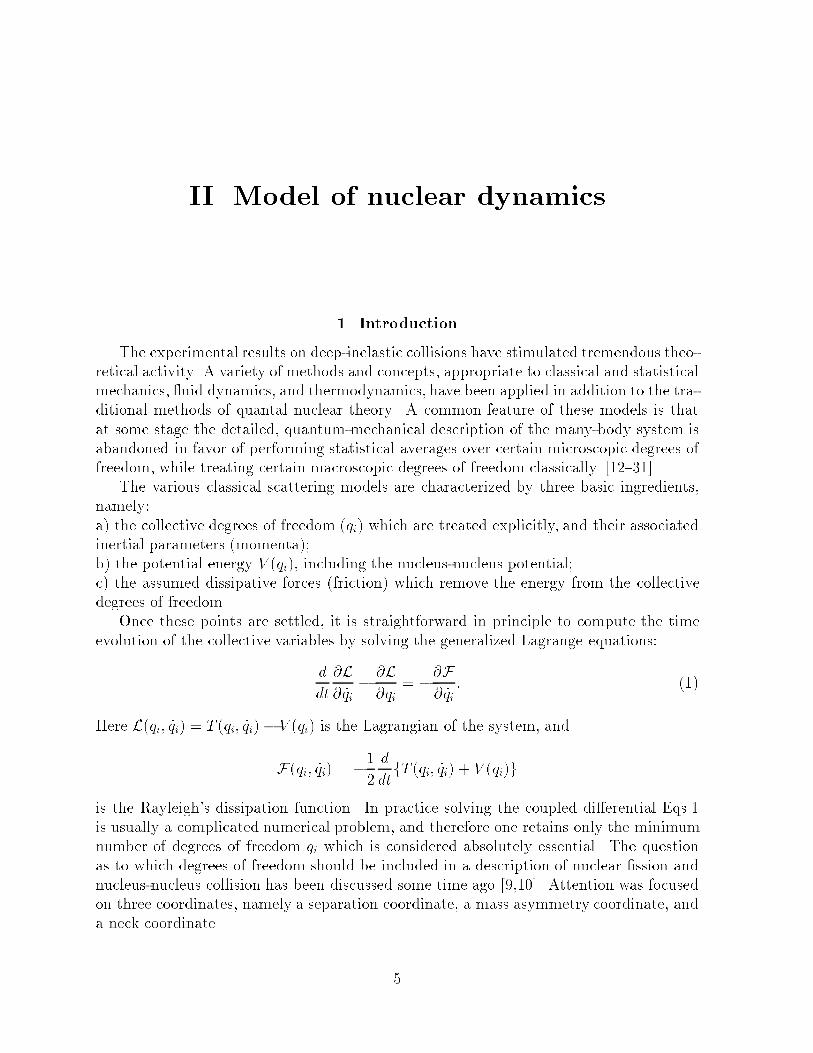
II. Model of nuclear dynamics1. IntroductionThe experimental results on deep-inelastic collisions have stimulated tremendous theo-retical activity. A variety of methods and concepts, appropriate to classical and statisticalmechanics, uid dynamics, and thermodynamics, have been applied in addition to the tra-ditional methods of quantal nuclear theory. A common feature of these models is thatat some stage the detailed, quantum-mechanical description of the many-body system isabandoned in favor of performing statistical averages over certain microscopic degrees offreedom, while treating certain macroscopic degrees of freedom classically. [12{31]The various classical scattering models are characterized by three basic ingredients,namely:a) the collective degrees of freedom (qi) which are treated explicitly, and their associatedinertial parameters (momenta);b) the potential energy V (qi), including the nucleus-nucleus potential;c) the assumed dissipative forces (friction) which remove the energy from the collectivedegrees of freedom.Once these points are settled, it is straightforward in principle to compute the timeevolution of the collective variables by solving the generalized Lagrange equations:ddt @L@ _qi � @L@qi = �@F@ _qi : (1)Here L(qi; _qi) = T (qi; _qi)� V (qi) is the Lagrangian of the system, andF(qi; _qi) = �12 ddtfT (qi; _qi) + V (qi)gis the Rayleigh's dissipation function. In practice solving the coupled di�erential Eqs.1is usually a complicated numerical problem, and therefore one retains only the minimumnumber of degrees of freedom qi which is considered absolutely essential. The questionas to which degrees of freedom should be included in a description of nuclear �ssion andnucleus-nucleus collision has been discussed some time ago [9,10]. Attention was focusedon three coordinates, namely a separation coordinate, a mass asymmetry coordinate, anda neck coordinate. 5

6 II. Model of nuclear dynamicsR

1l1 2l

r

2RFig 2.1 Parameterization of the nuclear shape(prescission shape). r is the distance betweencenters of spheres, R1 and R2 are their radii, andl1 and l2 are the widths of their segments beinginside the neck.max

θθFig 2.2 Window opening, | � = sin �sin �max .2. Shape parameterizationHere we brie y outline the shape parameterization of two colliding nuclei, which al-ready has been introduced in [7] and used in [3] and [6].The axially symmetric shapes of �xed volume consists of two generally unequal spheresmodi�ed by a smoothly �tted portion of a third quadratic surface of revolution. A set ofdimensionless degrees of freedom specifying the con�guration are the following (Fig 2.1and 2.2): 1) distance variable � = r=(R1 + R2);2) neck variable � = (l1 + l2)=(R1 + R2); (2)3) asymmetry variable � = (R1 �R2)=(R1 + R2):In the above, r is the distance between the centers of the spheres, whose radii are R1 andR2. The quantities l1, l2 are the distances from the inner tips of the two spheres to therespective junction points with the middle quadratic surface of revolution. The naturalboundaries of the con�gurational space (�, �, �) turn out to be given by [7]:� � j�j; �1 � � � 1; 2 � (1 + ��1)j�j � � � maxf0; 1� �g: (3)As may be readily veri�ed, the upper boundary for � corresponds to egg-like shapes forwhich the middle quadratic has just covered up completely the smaller sphere. At thelower boundary we have separated spheres for � = 0 and portions of intersecting spheres(without any middle quadratic surface) for � = 1 � �. At scission the center quadraticdegenerates into a cone, which implies �sc = 1 � ��1sc .In addition to the macroscopic variables (�, �, �) there are three rotational degrees offreedom (�1; �2; �rel) and three angular velocities (!1; !2; !rel) connected with the rotationof sphere 1 and sphere 2 and the rotation of the shape as a whole.As a parameter, which controls the transition from separate nuclei to compound nu-cleus, we introduce the window opening parameter � (Fig 2.2):� = sin �sin �max : (4)

3. Kinetic and potential energies; shell corrections 7λ

0 1

1

2 3

∆ = 0.3

ρFig 2.3 Shapes in (�; �)-space are shown for the �xed parameter � = 0:3. The straight line� + � = 1 corresponds to two intersecting spheres. There are no shapes under that line. Anotherline � = 1 � ��1 is the scission line. Con�gurations below this line are two separated fragments.The third line is upper boundary � = 2 � j�j(1 + ��1), which corresponds to the situation whensmaller of the spheres is enclosed by the neck. Con�gurations above this line consist of the part ofone sphere and the part of ellipsoid, which is the neck.3. Kinetic and potential energies; shell correctionsKinetic energy. The collective kinetic energy of gas or liquid is given byT = 12 Z �d(r) [u(r)]2 d3r = 12�d Zshape[u(r)]2 d3r; (5)where �d(r) is the matter density and u(r) the collective velocity at position r. In ourcase the matter density is uniformly distributed within the shape and zero outside. Thevelocity �eld u(r) has to be chosen in accordance with the collective degrees of freedom.The time-dependent changes of the shape result in a collective ow which rearrangethe matter to maintain a uniform density distribution. The boundary condition is thatthe velocity component normal to the surface is equal to the normal component of thesurface velocity. The assumption of incompressible irrotational ow together with theboundary condition de�ne uniquely the whole velocity �eld and thereby the kinetic en-ergy for the shape degrees of freedom. However, the solution of the resulting Laplaceequation is numerically too costly for practical applications. So it is convenient to use theWerner-Wheeler approximation [59]. It has been found that in the dynamical trajectorycalculations the motion in the � direction was invariably overdamped to such an extentthat the component of the inertia tensor Mij associated with � could be safely neglected.The kinetic energy is then reduced to the formT = 12M�� _�2 + M�� _� _� + 12M�� _�2: (6)

8 II. Model of nuclear dynamicsThe matrix element M�� of the mass tensor for two separated spheres is exactly thereduced mass.In the rotational degrees of freedom the kinetic energy is equal to:Tr = 12(Irel!2rel + I1!21 + I2!22); (7)where I1 and I2 are the rigid moments of inertia of sphere 1 and 2, respectively andIrel = Itot � I1 � I2 where Itot is the rigid moment of inertia of the whole system. Twospheres can rotate independently from the relative rotation, but due to the tangentialfriction, after some time all the frequencies !rel, !1 and !2 are more or less equal and thebody rotates as a rigid one.The mass tensor is calculated from Eq.5 and equal to (see, for example, [65])M%& = �d� Z �12B%B& + P 2A%A&� dz %; & = �; �;�; (8)where P = �� is the equation of the nuclear surface in cylindrical coordinates (��; z; �), andA% = � 1P 2 Z z @P 2@% dz0 � �V0 Z @P 2@% z00 dz00; (9)B% = �12 1P 2 @P 2@z Z z @P 2@% dz0 + @P 2@% : (10)V0 is the total volume of the systemV0 = � Z P 2 dz (11)Moments of inertia are given byItot = Irel + I1 + I2; (12)Itot = �d� Z �12P 4 + p2z2� dz � �d�2V0 �Z P 2z dz�2 ; (13)I1;2 = �d 4�15R51;2: (14)Potential energy. The potential energy of the shape under question is calculatedas a sum of the nuclear part and the Coulomb part. The nuclear part using a doublefolding procedure developed by Krappe, Nix and Sierk [60] can be written as:Vn = � Cs8�2r20a3 ZZ �1a � 2�� exp(��=a) d3r d3r0; (15)

3. Kinetic and potential energies; shell corrections 9where � = jr� r0j, Cs = as(1 � ksI2) and I = (N � Z)=A. The parameters r0, a, as andks are taken from the �t done in [60]. For axially symmetric shapes formula 15 reducesto the three dimensional integral of the following type:Vn = Cs4�r20 ZZZ 2 � "��a�2 + 2�a + 2# exp(��=a)! P2(z; z0)P2(z0; z)�4 dz dz0 d� ; (16)where P2(z; z0) = P (z) P (z)� P (z0) cos �� dPdz (z � z0)! ;�2 = P (z)2 + P (z0)2 � 2P (z)P (z0) cos � + (z � z0)2:A similar procedure has to be done in calculating the Coulomb part of the potentialwhich for an axially symmetric shape can be written as:Vc = �3 �z�z0 ZZZ P2(z; z0)P2(z0; z)� dz dz0 d�; (17)where �z and �z0 are the charge densities.Shell e�ects. The e�ect of shell structure on the nuclear deformation energyhas been understood in broad outline since the sixties and, in more quantitative detail,with the advent of the Strutinsky shell correction method. This macroscopic-microscopicmethod has provided useful insights into the role of shell e�ects. It has also served asthe basis for relatively accurate extrapolations into new domains of the periodic tableand nuclear deformations, complementing self-consistent calculations of the Hartree-Focktype.The importance of shell e�ects in the fusion of nuclei was demonstrated experimentallyas an enhanced fusion probability when using Pb or Pb-like targets from the transuranicregion. Shell e�ects are included in calculations in a phenomenological form proposedby Myers and Swiatecki [61], [8]. In that approach the shell correction S0(N;Z) to thepotential energy is written in the formS0(N;Z) = (5:8MeV) FN + FZ(A=2)2=3 � 0:325A1=3! ; (18)where FN = qN(N �Ni�1)� 35(N5=3 �N5=3i�1)with qN = 35N5=3i �N5=3i�1Ni �Ni�1 :Here Ni�1 and Ni correspond to the numbers of closed shell neutrons and N is the actualnumber of neutrons between Ni�1 and Ni for a system of mass A. The same formulas forFZ and qZ describe the shell e�ect for protons. For neutron and proton numbers N andZ corresponding to closed shells Ni�1 and Zi�1 the shell e�ect is strongest and is equal toS0(N = Ni�1; Z = Zi�1) = �5:8 � 0:325A1=3: (19)

10 II. Model of nuclear dynamicsFor example, in the case of 208Pb this gives about -11.2 MeV.The above shell correction S0(N;Z) refers to spherical shapes. For deformed shapesthe shell correction is attenuated according to [61], [8]:S(N;Z) = S0(N;Z) 1� 2dist2a2 ! exp �dist2a2 ! ; (20)where dist2 = Z d4� (r(�; �) �R0)2and r(�; �) is the radius vector describing the given shape and R0 is the radius of theequivalent sphere.One remaining problem is how to interpolate in a smooth way between the sum ofthe shell corrections S1 and S2 of the colliding nuclei in the entrance channel and theshell correction Sc of the compound shape. We adopted an interpolation in terms of thedegree of communication between the two nuclei as speci�ed by the \window opening"parameter � of [7], de�ned by Eq.4S = (1� �)(S1 + S2) + �Sc: (21)For separated shapes (below the scission line) alpha is equal to zero and we have onlyS1 + S2. When the neck loses its concavity at � = 1 the shell correction is equal to thecompound nucleus shell correction Sc, and this is used for convex shapes with � > 1.Here we do not consider that shell corrections attenuate with growing temperature aswas done in [62]. 4. Equations of motionIn this section we introduce the dynamical deterministic equations of motion.Generic deterministic equation. The system is described by the classicalRayleigh-Lagrange equations 1 with the following ingredients:L = 12 _qM _q � V (q) (22a)F = 12 _q� _q; (22b)where M is the mass tensor and � the dissipation tensor. If one de�nesx � q_q ! ; v � _q�M�1( _M + �) � @qV (q) ! ; (23)where @q is the gradient operator, then Eq.1 can be rewritten as_x = v: (24)We call Eq.24 a generic deterministic equation to distinguish it from stochastic equationof motion where the stochastic noise term is added.

4. Equations of motion 11In our case the quantities q form the set of the macroscopic variables q =(�; �;�;�Z; �; �1; �2). The �rst three are the shape parameters, the last three are rota-tional degrees of freedom and �Z is an additional degree of freedom, charge asymmetry,equal to Z1=31 �Z1=32Z1=31 +Z1=32 . We consider the motion in � and �Z directions to be overdamped.So altogether there are �ve second order and two �rst order di�erential equations.Dissipation. The tensor � in Eq.22b is a dissipation tensor, which can be foundafter de�ning the mechanism of the energy dissipation. We restrict ourselves to one-bodydissipation [11], arising from collisions of independent particles with the moving boundaryof the nucleus. In the one-body dissipation model [11], the energy ow from collectiveto intrinsic motion is attributed to the interaction of individual nucleons with the mean�eld produced by all nucleons in the system. In a simpli�ed picture this interaction maybe viewed as mediated by collisions between nucleons and a moving container wall, or bythe passage of nucleons from one fragment to the other through a window.There are two limiting cases in which two di�erent simple formulas for the rate of thedissipated energy can be derived. The �rst one is so called the mononuclear regime whenthe system of colliding ions can be considered as a monosystem with a thick neck. Inthat case the gas of nucleons can be considered as a relaxed Fermi gas and the rate of theenergy dissipation is given by the following wall formula [11]:_Ewall = �m�v I dS ( _n�D)2; (25)where �m is the mass density of nucleons, �v is their average speed (equal to three quartersof the Fermi velocity in the Fermi gas model), dS is an element of nuclear surface, _n is thenormal velocity of walls and D is the overall drift velocity of the gas of nucleons ensuringthe invariance of Eq.25 against translations and rotations.In the second limiting case, the dinuclear regime, when two ions are either separatedor connected by a thin neck, Eq.25 can not be applied as we are dealing with two Fermigases separated by the collective velocity. In that case the so-called \wall plus window"formula can be applied and it reads as follows:_Ew+w = �m�v Z1 dS ( _n�D1)2 + �m�v Z2 dS ( _n �D2)2 + 14�m�vSw(u2t + 2u2r) + 169 �m�vSw _V 21 :(26)The �rst two terms correspond to the wall formula (Eq.25) but are calculated for eachfragment separately with drift velocities D1 and D2 for each of the gases. The third termis associated with the dissipation due to the exchange of particles through the windowof the area Sw. The components of the relative velocity of two fragments ut and urcorrespond to the velocities parallel and perpendicular to the window. The last termin Eq.26 corresponds to the dissipative resistance against the asymmetry changes [63],[64] with _V1 being the rate of the change of the volume of fragment 1. Eqs.25 and 26express the rate of the dissipated energy in the two limiting cases of the mononuclear anddinuclear regimes. In general when the situation is in between these two limiting cases asmooth transition between formulas 25 and 26 is used [3]:

12 II. Model of nuclear dynamics_E = f _Ewall + (1� f) _Ew+w (27)with a form factor f going to 1 for sphere or spheroid like shapes and to 0 at scission.Eq.27 is the additional dynamical equation which can be added to the generic deter-ministic equation (24) describing the evolution of the collective coordinates.There is another equation, for the time derivative of the di�erence in the excitationenergies of both parts of the nuclear system:ddt(E�1 � E�2) = _E1 wall � _E2 wall + 2T0 _S21; (28)where �rst two terms are de�ned in previous subsection and the last one is due to thetemperature feedback with T0 = (T1 + T2)=2 being the average temperature of the �rstand second fragment. _S21 is the entropy ux taken from Feldmeier [65].5. FluctuationsIn this section we present how to introduce uctuations into deterministic equationsof motion as well as how to connect their magnitudes to dissipation in speci�c situations.Fokker-Planck equation. Let Q and q denote collective and intrinsic degreesof freedom, and P and p their associated momenta correspondingly. Assume an inertiaM for the collective coordinate, and m for the internal 1. Hamiltonian dynamics for anensemble of trajectories F (Q;P; q; p; t) can be described by the Liouville equation:@F@t = LF; (29)where L = � PM @@Q + @H@Q @@P � pm @@q + @H@q @@p;and H is the Hamiltonian of the system.If we want to describe the system by only collective variables, we follow the distributionf(Q;P; t) = R dq dp F (Q;P; q; p; t). The equation for f(Q;P; t) can easily be found:@f@t = � PM @f@Q + @@P *@H@Q+ f! : (30)We used here that @2@p @qH = 0, F ! 0 when Q or P !�1 and de�nitionh�i � R dq dp (�) F (Q;P; q; p; t)R dq dp F (Q;P; q; p; t)Now we would like Eq.30 not to depend on F . Let us consider Q to be slow parametersand assume that the evolution of the fast variables q under H is chaotic and ergodic when1We will deal with this variables as if they were one-value quantities. Generally speaking, theyare not, but the generalization can be achieved easily.

5. Fluctuations 13Q is held �xed. We also assume that the time required for the Hamiltonian H to changesigni�cantly is much bigger then the Lyapunov time associated with the fast chaos. Sothe last term in Eq.30 contains information about the average drift and di�usion in the Pdirection. The average drift could be in the form of a conservative force, @V (Q)@Q , plus aterm caused by coupling to the internal degrees of freedom, G, which (we will show later)is a dissipative term. Then Eq.30 takes the Fokker-Planck form:@f@t = lf + @@P (Gf) + 12 @2@P 2 (Df); (31)where l = � PM @@Q + @V@Q @@Pis the Liouville operator.Now let us take an initial distribution which is uniform on a single energy shell in thefull phase space (slow + fast degrees). We will call this distribution FU(Q;P; q; p), wherethe subscript U speci�es the total energy:FU(Q;P; q; p) = �[U �H(Q;P; q; p)]; (32)Under time evolution, the distribution FU will not change (Liouville's theorem): LFU = 0.When we project out the fast degrees of freedom, we get:fU (Q;P ) = Z dq dp �[U �H(Q;P; q; p)]: (33)But if we view the slow degrees of freedom as "parameters" which determine the Hamilto-nian for the fast degrees, then the right side of Eq.33 just represents the density of statesof the fast degrees, when the slow ones are "frozen" at (Q;P ). So: fU (Q;P ) = � , where� is the density of energy states in Eq.31 above. Now we demand that the Fokker-Plankequation (31) has the property that fU is invariant with time, because FU is invariantwith time [46]. Due to the fact that lfU = 0 we �nd:@@P (G�) + 12 @2@P 2 (D�) = 0;and G = � 12� @@P (D�): (34)Hence one can rewrite the Eq.31:@f@t = lf + 12 @@P "�D @@P f�!# : (35)This Fokker-Planck equation is analogous to the energy di�usion equation derived byC.Jarzynski [48{51].

14 II. Model of nuclear dynamicsDerivation of uctuating force. In the absence of coupling of the collectivemotion to the internal degrees of freedom of the nucleus, the evolution in (Q;P )-space isgoverned by the following deterministic, conservative equations of motion:dQdt = PM ; dPdt = �dVdQ: (36)An ensemble of trajectories evolving under these equations may then be described bya phase space density f(Q;P; t) which evolves according to the Liouville equation:@f@t = � PM @f@Q + dVdQ @f@P : (37)When we allow for coupling to the internal nucleonic degrees of freedom, then thelatter act as a kind of a heat bath, exerting both a dissipative and a uctuating force onthe collective degree of freedom. The e�ects of these forces may by described by addinga term to the evolution equation for f , which now becomes a Fokker-Planck equation:@f@t = � PM @f@Q + dVdQ @f@P + 12 @@P "�D @@P f�!# : (38)Here, � denotes the density of states for the nucleonic degrees of freedom, and D isa momentum di�usion coe�cient. The form of the last term in Eq.38 is determined bydetailed balance. This last term may be easily rewritten as follows:last term = � @@P " 12� @@P (�D)f# + 12 @2@P 2 (Df) = � @@P (Ffricf) + 12 @2@P 2 (Df); (39)where Ffric � �G = 12� @@P (�D): (40)The quantity Ffric plays the role of a momentum drift term, that is, an average forceresulting from the coupling to the nucleonic "heat bath". We now show explicitly thatFfric has the form of a frictional force.The total energy of the collective + internal degrees of freedom may be written as:E = P 22M + V (Q) + E�; (41)where E� is the excitation energy of the internal degrees of freedom. Since the totalenergy E is conserved, we can treat the excitation energy E� as a function of Q and P -E� = E�(Q;P ) - which implies that, for �xed Q,@@P = � PM @@E� : (42)We can then write the average force, Ffric, exerted by the internal degrees of freedomon the collective degree, as:

5. Fluctuations 15Ffric = � 12� @@E� (�D) PM = � _Q; (43)where _Q � dQ=dt = P=M , and = 12� @@E� (�D): (44)Eq.43 reveals us that Ffric is indeed a friction-like force, whereas Eq.44 is a uctuation-dissipation relation between the friction coe�cient , and the momentum di�usion coef-�cient D.Since the nucleonic degrees of freedom form a many-particle system, the density ofstates �(E�) grows very rapidly, as a function of excitation energy E�. (Roughly, � �epE.) Thus, for su�ciently large excitation energy, the derivative appearing in Eq.44 maybe dominated by the derivative of �, i. e. we may treat D as a constant and with thisapproximation, we get � D2 @@E� ln � = D2T ; (45)where T is the temperature of the nucleus. Equation 45 is a version of the Einsteinrelation, originally derived for Brownian motion.The Fokker-Planck approach outlined above is appropriate for the description of anensemble of trajectories in the collective coordinate phase space. In a numerical simulationof a single trajectory, we take a Langevin approach instead. Then the equations of motionfor the trajectory look like the following:dQdt = PM ; dPdt = �dVdQ + Ffric + ~Ffluc: (46)Here, Ffric = � _Q is computed, for instance, with the wall formula [11], whereas~Ffluc is a rapidly uctuating stochastic force. This stochastic force is responsible forthe momentum di�usion described by the coe�cient D(Q;P ). The force ~Ffluc may besimulated numerically, by repeatedly giving the collective momentum a random kick, �P ,i. e. a discontinuous change in the collective momentum. The value of �P is chosenrandomly from a Gaussian distribution, with a mean value and variance given by:�P = 0 (47)(�P )2 = D �t (48)where �t is the (small) time step between kicks.The same result (Eq.45) one can obtain using only Lagrange and Langevin equationsand not incorporating ensemble distribution equations as shown in [57].Di�usion term for Fermi particles. In the more general case, where we do nottreat D as a constant, equation 44 may be inverted to yield the following expression forthe momentum di�usion term, in terms, of the friction coe�cient:

16 II. Model of nuclear dynamicsD = 2� Z E�0 dE � : (49)The wall formula for one-body dissipation gives the rate of energy transfer from thecollective to the nucleonic degrees of freedom as:dE�dt = ��v I da _n2; (50)where � is the mass density of the nucleus, �v is the average speed of nucleons, and the�nal factor on the right side is an integral, over the surface of the nucleus, of the square ofthe normal outward velocity of a surface element. For a given surface element, _n can bewritten as _Q @n=@Q, where (@n=@Q) dQ gives the normal outward displacement of thesurface element accompanying an in�nitesimal change dQ in the value of the collectivecoordinate. Since the rate at which energy is dissipated is equal to _Q2(= �Ffric _Q),we get, after dividing both sides of 50 by _Q2, the following expression for the frictioncoe�cient: = ��v I da @n@Q!2 � �v � I(Q): (51)(Note that �v, the average nucleonic speed, is a function of excitation energy.) We thenhave the following expression for the momentum di�usion coe�cient:D = 2I� Z E�0 dE ��v: (52)We treat D as a function of both Q (since I depends on Q), and P (since the excitationenergy is determined from P , for a given Q).If the excitation energy satis�es two conditions: 1) E� � "FA1=3 and 2) E�� "FA�1then it is appropriate to use the formula for level density of Fermi gas [54]:� = 61=412 g0(g0E�)5=4 exp8<:2 �26 g0E�!1=29=; ; (53)where g0 � g("F ) � 32 A"F is a sum (protons and neutrons) of the density of one-particlelevels on the Fermi surface and "F is the Fermi energy. The temperature is given by:T�1 = 1� @�@E� = �54E��1 + �26 g0E�!1=2 (54)Supposing that �v does not change too much with growing E� one obtains:D = 8I�vE� ��1 + �1=4 exp ���1=2�Er� ���1=4�� ; (55)where � = 2�23 g0E� and function Er� is the imaginary error function de�ned as: Er�(x) =2p� Z x0 et2dt.

5. Fluctuations 17Langevin approach. Let x(t) be an evolution trajectory of a system governed bydeterministic rule _x = v(x; t). If stochasticity of the system is taken into account thenlet �(x; t) be a white Wiener noise 2. with a mean value being zero: h�(x; t)i = 0 andcovariance h�(x; t) �(x; t+ s)i = D(x; t)�(s);where D is the covariance matrix and the sign corresponds to matrix multiplication.An ensemble of systems is de�ned by distribution function f(x; t). We consider quantitiesx; v; �; @x � @@x to be vectors and D a matrix. Then the system can be described by 4possible equations (@t � @@t):Deterministic dynamics Stochastic Wiener noise process1) generic deterministic equation 3) Langevin equation_x = v _x = v + �2) Liouville-like�) equation 4) Fokker-Planck equation@tf = �@x(vf) @tf = �@x(vf) + 12@2xx(Df)�) This equation is exactly Liouville's only in case of nondissipative Newtonian dynamics.In this subsection we would like to argue why we choose Langevin approach for studythe dynamical system.The �rst two approaches are completely deterministic. They allow us to certain esti-mate properties of the system. For example, given a model of colliding nuclei, one cancalculate extra-push, extra-extra-push energies, averages of excitation energy, nucleonstransfer and so on. However, they do not give a probabilistic description of what weobserve in experiments. Therefore we use the probabilistic approach, which allows us todeal with distributions and ensembles. This is accomplished with the random force in theLangevin equation or di�usive term in the Fokker-Plank equation (FPE)3.2We use the term \white Wiener noise" to point out that the stochastic noise has no timememory and is described by Wiener di�erential [68]; which means that in equation dx = v dt +� dW the following is satis�ed h�t�t+si � �(s) and dW 2 = dt and h�ni = 0, when n > 2.3It is worthwhile to note that there are two interpretations of the Langevin equation and, hence,two types of FPE. One is Ito's representation, where it is assumed that ddt� = @@t�. The otherone is Stratonovich's, where ddt� = @@t� + _x @@x� [56] . Klimontovich [58] distinguishes yet the\kinetic form" of FPE.

18 II. Model of nuclear dynamicsIn previous subsections we used the FPE to establish the uctuation-dissipation rela-tion from the condition of detailed balance [55]. But in practical implementation (numer-ical calculations) the use of the FPE is problematic because the dynamical descriptiondemands a parameterization of the distribution. And the number of parameters growsexponentially with the dimensionality of the phase space (x-space). For instance, in thesame model of heavy-ion collisions, the con�gurational space is of dimensionality 4; con-sider 2 directions to be overdamped; plus 1 dimension of excitation energy. Altogether 7.It is clear that numerical evolution of the FPE is almost impossible to the appropriateorder of precision. Thus we are left with the Langevin equation only.Implementation of the Langevin equation. Let us summarize the derivationof the appropriate Langevin equation.The starting point is the deterministic macroscopic equationh _xi = v(hxi) (56)describing the average behavior of the collective coordinates. Adding the noise we obtainthe \microscopic" stochastic equation:_x = v(x) + �(x; t): (57)However h _xi = hv(x)i 6= v(hxi) (58)in the general case. Fortunately, the choice of the Lagrangian L and Rayleigh dissipationfunction F in the form 22a cause the equation of motion to be linear. So the equalityhv(x)i = v(hxi) holds.The next step is the determination of the stochastic force �(x; t). The linearity of thefriction term sets the condition of white noise: �(t)�(t + s) � �(s). The assumption thatmicroscopic uctuations are small over in�nitesimal intervals of time says that this noiseis of Wiener type.One can treat Eq.57 as a simulation of the corresponding FPE. We have derived therelation between the di�usion coe�cient D in Eq.38 and the friction force (Eq.40). Henceusing the Ito representation one gets:x(t + �t) = x(t) + v(x(t))�t + Z t+�tt �(x(t); t0) dt0 (59)with h�(x; t)�(x; t + s)i = D(x)�(s) or � dt = D dW; (60)where dW is the Wiener di�erential (dw2 = dt). The di�usion term in the correspondingFPE is 12 @@x!2Df: (61)

6. Additional topics 19Alternatively, we can use the Stratonovich representation:x(t + �t) = x(t) + v(x(t))�t + Z t+�tt �(x(t0); t0) dt0 (62)with h�(x; t)�(x; t + s)i = C2(x)�(s): (63)The integral in the last term in Eq.62 is presented as:12h�(x(t); t) + �(x(t + �t); t+ �t)i�t;which is not very convenient since one has to know � at the next point of integration.The di�usion term in the corresponding FPE12 @@xC!2 f = 12 @@x!2C2f � 12 @@x Cf @@xC! : (64)consists of an additional systematic friction-like part.Ito representation is simpler to use than the Stratonovich one. However, both ap-proaches are equally valid. 6. Additional topicsExchange of particles. When the atomic nucleus is idealized as a system ofweakly interacting nucleons in a time-dependent mean-�eld potential well, the nature ofthe macroscopic dynamics describing the time evolution of the nuclear shape is believedto be intimately related to the nature of the nucleonic motions inside the nucleus. Herewe concentrate our attention on the motion of nucleons through a small window area �(dinuclear regime). One of the e�ects of such a motion is the dissipation in macroscopicdegrees of freedom described by the window formula. Another e�ect is uctuations innumber of exchanged particles. These uctuations are not connected to the thermal uctuations considered above and touch only one degree of freedom | asymmetry. Weassume that the motion of nucleons is chaotic and the correlation time is in�nitesimallysmall. Then for su�cient small period of time the process of exchanging nucleons can betreated as a Poisson process. And because of �nite number of particles the distributionundergo the binomial law. Let us consider the number of particles own from nucleus 1to nucleus 2 during a time interval �t to be N1 and from 2 to 1 to be N2. Then the changeof the atomic mass number of nucleus 1 is equal to:�A1 = g = N2 �N1 (65)This quantity can be rewritten as a sum of average term and uctuating term with zeromean value: �A1 = ~g = �g + �L ; h�Li = 0 (66)

20 II. Model of nuclear dynamicsThe di�usion coe�cient DA is de�ned by relation:h�L2i = DA�t = h~g2i � �g2 (67)Quantities N1 and N2 are independent and are taken from binomial distributions. So, thefollowing equivalencies:hN1N2i = hN1ihN2i and hN2i i = hNii2 + hNii 1� hNiiAi ! (68)lead us to the explicit expression of h�L2i:h�L2i = hN1i+ hN2i � hN1i2A1 + hN2i2A2 ! (69)We denote A1 and A2 atomic mass numbers and A = A1+A2. It has been shown [11,63,66]that the average number of exchanged particles is given by:hN1i � hN2i � 14��vn�t; (70)where �v is the average particle speed and n is the concentration of particles { number perunit volume. This gives us immediately the expression for DA:DA = 12��vn� 116a�2�v2n2�t here a = A1A2A1 + A2 : (71)The limit when two containers can be treated as in�nite reservoirs of particles is achievedwhen the time interval �t is small enough:�t� 8a��vn (72)Going to our asymmetry variable � we use the following relations:_� = f _A1; D� = f2DA; (73)where f = @�@A1 �����A = 23A A�2=31 A�2=32(A1=31 + A1=32 )2 (74)In Chapter IV we will see what contribution the uctuations of this kind give to thedynamics; and how they are important in comparison to thermal uctuations.Dissipative uctuations. The same scheme can be applied to the uctuationsconnected to collision of nucleons with the wall of the container. In derivation of wall andwindow formulae there have been used only the average quantities. We take into accountthat the number of particles colliding with the wall and the number of particles crossingthe window can uctuate.

6. Additional topics 21Fig 2.4 The potential shown on (�;�0Z)-subspace, [X-axis �=(-0.5,0.5) and Y-axis �0Z=(-0.05,0.05) ], for the system 86Kr+136Xe in thepoint � = 1:26, � = 0:05, which corresponds tothe shape at the beginning of the trajectory whennuclei just start to feel nuclear interaction. Thereare no shell included. Contour lines correspond tolevels of the potential energy in MeV with respectto the potential energy of separated nuclei.

x

y

a

b 8

9

5

17

2

3

3’

4

6

Fig 2.5 We choose points to determine the coef-�cients in polynomial expansion of the potentialaround (0,0)-point in (�;�Z)-subspace. Point 1is the center of coordinate system.Parameterization of the potential. In the above the dynamical coalescence andreseparation model was described. This model is more realistic then the schematic one weuse in Chapter III to test methods of calculating small probabilities. Simulations madewith a more realistic model are time-consuming due to the fact that the potential doesnot have simple analytic form and can be presented only as a three-dimensional integral,Eqs.16 and 17. Each trajectory in numerical simulations consists of hundreds points; andat each point one has to calculate conservative forces in four directions { (�; �;�;�Z).It is clear that calculation of millions of trajectories, for di�erent reactions and su�cientstatistics, becomes in practice impossible.Here we propose the way which can speed up the calculations. Let us parameterizethe potential to avoid calculation of three-dimensional integral4. The simplest way is tomake the four-dimensional lattice in the phase space. Then having values of the potentialon the lattice one can interpolate the value in any intermediate point. Simple estimationshow that a lattice of size 1004 takes about 200 Mb of the computer memory and a lotof time to calculate the potential. We can use the property that the potential energyis symmetric under transformation (�;�Z) ! (��;��Z). First, let us note that theparameter �Z is strongly related to � i.e. the potential grows fast when going fromminimum in direction (� = 1;�Z = �1) and grows slowly in direction (� = 1;�Z = 1).So, let us choose new parameters (�;�0Z), where �0Z = �Z ��. This pair of parameters4An analogous parameterization of the conservative forces for the same model is in [69].

22 II. Model of nuclear dynamicskeeps the same property of symmetry. If we do not take into account shell e�ects then thepotential around the point (� = 0;�0Z = 0) looks like a smooth potential well (See Fig.2.4) in the directions x = � and y = �0Z. Therefore we have chosen parameterization inthat subspace as a 4'th degree polynomial:z = f1 + f2x2 + f3xy + f4y2 + f5x4 + f6x3y + f7x2y2 + f8xy3 + f9y4: (75)This is the expansion of the potential z around (0,0)-point. The symmetry propertyeliminates the odd degree terms. The potential in the subspace (�,�) is parameterized bya bilinear interpolation of the lattice points. Eq.75 can be rewritten:z = ~f � ~p(x; y); (76)where ~p(x; y) = (1; x2; xy; y2; x4; x3y; x2y2; xy3; y4)and ~f = (f1; f2; f3; f5; f6; f7; f8; f9). Now let us choose the 9 points as shown on Fig.2.5giving the values ~z = (z1; z2; z3; z5; z6; z7; z8; z9). Then the coe�cients ~f can be found fromthe equation: M � ~f = ~z; (77)where M = 0BBBBBBBBBBBBBBBBBBB@~p(0; 0)~p(a; 0)~p(0; b)~p(a; b)~p(a;�b)~p(a2; b2)~p(a2 ;� b2)~p(3a2 ; b2)~p(3a2 ;� b2)

1CCCCCCCCCCCCCCCCCCCA = 0BBBBBBBBBBBBBBBBBBBB@1 0 0 0 0 0 0 0 01 a2 0 0 a4 0 0 0 01 0 0 b2 0 0 0 0 b41 a2 ab b2 a4 a3b a2b2 ab3 b41 a2 �ab b2 a4 �a3b a2b2 �ab3 b41 a24 ab4 b24 a416 a3b16 a2b216 ab316 b4161 a24 �ab4 b24 a416 �a3b16 a2b216 �ab316 b4161 9a24 3ab4 b24 81a416 27a3b16 9a2b216 3ab316 b4161 9a24 �3ab4 b24 81a416 �27a3b16 9a2b216 �3ab316 b416

1CCCCCCCCCCCCCCCCCCCCA (78)The exact solution for ~f is the following.f1 = z1;f2 = �18z1 + 18z2 � 2z3 + z4 + z5 + 2z6 + 2z7 � 2z8 � 2z912a2 ;f3 = �z4 + z5 + 16z6 � 16z76ab ;f4 = �42z1 � 18z2 + 2z3 � 3z4 � 3z5 + 30z6 + 30z7 + 2z8 + 2z912b2 ;f5 = 6z1 � 6z2 + 2z3 � z4 � z5 � 2z6 � 2z7 + 2z8 + 2z912a4 ; (79)f6 = �3z6 + 3z7 + z8 � z93a3b ;

6. Additional topics 23f7 = 2z1 � 2z2 � 2z3 + z4 + z52a2b2 ;f8 = 2z4 � 2z5 � 5z6 + 5z7 � z8 + z93ab3 ;f9 = 30z1 + 18z2 + 10z3 + 3z4 + 3z5 � 30z6 � 30z7 � 2z8 � 2z912b4 :This simple trick greatly speeds up the calculation especially when we need to getsu�cient statistics.

III. Computation of small probabilities1. IntroductionIn the world of microphysics experimental results are often presented in form of thedistributions of the measured quantities and not as a precise values of these quantities.This re ects the statistical nature of physical phenomena. In nuclear physics, due tothe microscopic and quantal nature of nuclei, probabilities and statistical distributionsbecome very relevant. If one takes radioactive decay, for example, it is well known thatthe nuclear ensemble does not decay at a de�nite time but is spread over time accordingto the exponential decay law.One way to attack the problem theoretically is to use a Monte Carlo method whichis very often applied in multidimensional problems. Using Monte Carlo simulations onecan e�ciently estimate distributions of values we are interested in, in regions of the mostprobable outcomes. However, sometimes it is important also to calculate distributionsand probabilities of rare outcomes. The direct simulation method in this case becomesimpractical. This chapter is devoted to that problem.Experimentalists are able to measure probabilities down to 10�35. It is obvious thatno one can calculate such values using direct methods of Monte Carlo. So it is importantto have methods capable of giving results comparable with the experimental data. Theproblem of calculating small probabilities was also studied in di�erent �elds. It plays asigni�cant role in chemistry [32{41].The probability. Each realization of a stochastic process (trajectory) is de�ned bya sequence of random numbers. So one is able to estimate (analytically or numerically)how probable one trajectory is, in comparison to others. That means that each trajectoryhas its own statistical weight p which we suppose to be known. The probability of someoutcome B is the ratio of the integral over realizations leading to B, to the integral overall possible realizations: PB = RB p(�) d�R p(�) d� ; (80)where � is an index de�ning a trajectory uniquely.24

2. Polymer method 252. Polymer methodPolymer analogy. A particularly simple and convenient way to describe a stochas-tic physical process is the Markov description. If one uses a Markov chain of states as astochastic description of the transition path, then the path can be treated as a polymerin which subsequent beads represent states of the system at subsequent time slices. Theanalogy between such a polymer and randomly accelerated particle is well known. Thetransition probability between neighboring states (beads) de�nes an ensemble of represen-tative paths or polymer con�gurations. This analogy suggests two novel computationalapproaches to stochastic process. The �rst is the possibility to sample the ensemble ofrealizations by moving the whole path through the phase space according to the de�neddistribution. The second is the possibility of rewriting the problem of calculating proba-bilities, as the problem of calculating Helmholtz free energies for a polymer thermalizedby a heat reservoir. In this approach, di�erent conditions of the process correspond todi�erent free energies. For instance, the equation 80 can be written down as:PB = e�(FB � F ); (81)where FB is the free energy of the polymer constrained by the condition B (in our case thiscondition is that the last bead correspond to the stage B), and F is the free energy of theunconstrained polymer. As will be shown below the free energy concept arises from theanalogy between the statistical distribution of trajectories and the canonical distributionof polymer con�gurations.Action. The Markov chain representing the path can be described by an action,analogous to a discretized quantum path integral action [52]. If � is a given realization ofa process (a given con�guration of the polymer) then one can write down the statisticalweight p(�) as: p(�) = e�S(�): (82)The value S(�) depending on the con�guration variable � is called an action. One cantreat this value as the energy of the polymer in the con�guration �. The distributione�S(�) corresponds to a canonical Boltzmann distribution with temperature equal to 1.For a Markovian chain p(�) is a product of statistical weights for subsequent time slicesand in S(�) this is a sum of subsequent actions (additivity).The free energy is given by:e�FC = ZC e�S(�) d�; (83)where C is a �xed external condition constraining the polymer. The de�nition 83 imme-diately leads to equation 81.Metropolis sweeps. By changing simultaneously the entire con�guration of thepolymer in a proper way one can sample the canonical distribution e�S(�). This algorithm

26 III. Computation of small probabilitiesis known as Metropolis Monte Carlo algorithm. Let us de�ne the probability of changingcon�guration � into con�guration � in this way:P (�! �) = ~P (�! �) + �(�� �)R(�): (84)The �rst term ~P (�! �) = �(�; �) min[1; e�(S(�)�S(�))] (85)is the Metropolis Monte Carlo probability rule [42] with a generating probability �(�; �)and acceptance probability min[1; e�(S(�)�S(�))]. The second term in 84 is the probabilityof rejecting a trial move: R(�) = 1� Z ~P (�! �0) d�0: (86)The generating function �(�; �) has to satisfy two conditions. The �rst is that thefunction � should be symmetric and should not change the measure of space, i.e. if weput ~P (� ! �) = �(�; �) then the exploration of phase space should be uniform. Thesecond is that the function � should generate ergodic, i.e. exhaustive, exploration of thespace.The Metropolis rule allows us to avoid the explicit calculation of the rejection prob-ability, R(�). The only consideration is the e�ciency, which strongly depends on thegenerating distribution �(�; �). A new chosen con�guration y should not be too close tox, otherwise exploration of the phase space will be too slow. On the other hand if chancesthat S(y) � S(�) are high then the number of rejections predominates over acceptationsand changes of con�guration occur rarely.The probability P (�! �) is normalized by de�nitions 84-86 and conserves the canon-ical ensemble: Z d� e�S(�)P (�! �) = e�S(�) (87)Computation of work. Equation 81 immediately leads to the following methodof calculating PB. The di�erence in free energy is equal to the work which needs to bedone to constrain the polymer to the condition B in an adiabatic way [43].Let us �rst introduce a new parameter � which changes from 0 to 1 and corresponds toan unconstrained polymer when � = 0, and constrained with a condition B when � = 1.Now let us choose a sequence of conditions which continuously switches the parameter� from 0 to 1. When � is changing in�nitely slowly then the total work performed onthe system is equal to the Helmholtz free energy di�erence. In this case the system is inquasistatic equilibrium with the reservoir (having temperature equal to 1) throughout theswitching process . Hence: �F = Z 10 d� *@S�@� +� : (88)This result is a well-established identity [44].

2. Polymer method 27For example, we are interested in the case when the last bead of the polymer is insidea region B. We can compose the sequence of states where the last bead is con�ned withina box with hard walls. Initially the box is so big that the polymer is considered to beunconstrained. Then the box shrinks slowly toward the region B (Fig 3.1).Of course, practically we can not reach the adiabatic limit. And each simulation wouldgive us di�erent result of performed work W . The relation of free energy di�erence andperformed work in nonequilibrium regime was recently found out by C.Jarzynski [45], [47]:�e��W� = e���F; (89)where � is the reversed temperature (equal to 1 in our case) and the average is de�nedover an ensemble of independent simulations.x0

xN

B

Fig 3.1 Schematic presentation of the process ofconstraining the polymer in the region B. Ini-tially the box is so big that the polymer is consid-ered to be unconstrained. Then the box shrinksslowly toward the region B. xB

5

4

3

2

1

x0Fig 3.2 Simple analytic model of a free fallingparticle being kicked in horizontal direction. Thequestion is: what is the probability that the par-ticle ends beyond the border xB.Advantages and disadvantages of the polymer method . Once the algorithmof the calculations is set then the computing e�ort does not depend on how small theprobability of interest is. One can calculate equally well either some value of probabilityor a value of several orders of magnitude smaller as the process of calculating work Wdoes not depend on the value of �F . This is the main advantage of the polymer method.Changing the external parameter � in an adiabatic way means that the polymer is inequilibrium in each moment of time. In other words, the characteristic time of polymerrelaxation is much smaller then the characteristic time of parameter changing. The poly-mer explores the phase space at each intermediate value of �. This implies a large numberof evaluations of S(�) for di�erent con�gurations of the polymer. So if the calculation ofS(�) takes, say, several minutes then the method becomes almost impractical.Another di�culty appears when the potential energy of the polymer has a non-triviallandscape. In this case the relaxation time of the polymer is the time needed for it to

28 III. Computation of small probabilitiesexplore all local minima. If barriers separating local minima are high enough then theprobability of passing through a barrier is small and the characteristic relaxation timebecomes extremely large.One solution to this problem is to use \smart" function �(�; �) which allows long-ranged jumps to penetrate barriers. This function must have information about potentialrelief and this makes the task depend on the speci�c situation5.Another way to deal with the problem is to divide the potential surface into localminima regions (if it is possible, of course, to divide it into regions between which theprobability of passing is negligible) and calculate the work separately for moving thepolymer from one potential well to another. Often the algorithm of calculating the workW is such that W can only grow up to the point after which the polymer quickly relaxes tothe new state | falls into the next potential well. While falling the polymer does negativework which is not taken into account. To account for this, one can calculate the work inreverse direction. So the true quantity W will be the di�erence: W = Wforth �Wback.The third way is to lift the main (absolute) minimum in potential energy so that itwould be comparable with the other minima. Then making the usual direct simulationsof the stochastic process we calculate probabilities of di�erent outcomes. And �nallywe compensate the real probability by the factor e�W , where W is the work done whenchanging the potential. For example, if there are two possible outcomes of the stochasticprocess A and B, computation of the work gives the quantity W and simulations with themodi�ed potential give probabilities P 0A and P 0B of events A and B. The real probabilitiesPA and PB can then be expressed as:PBPA = e�(FB�FA) = e�(FB�F 0A)�W = P 0BP 0A e�W ; (90)where FA, FB are free energies for conditions A and B, and F 0A is free energy with thelifted potential energy in the region A.3. ExamplesAnalytically solvable model . It is instructive to show how the method works ina simple exactly solvable model. Let us choose the process of discrete steps with Gaussiandeviation: P (xi+1) = N exp�(xi+1 � xi)22�2 ; x0 = 0: (91)The trajectory is presented as a set of N numbers fxiji = 1; :::; Ng. This process isactually the simulation of a pure Wiener process which also will be considered later inthis chapter. We can look at this process as a free particle falling down with a constantspeed with stochastic kicks in the horizontal direction (Fig.3.2). As a small probability5Remember that the function � has to satisfy the two conditions mentioned above (just afterEq.86).

3. Examples 29event let us de�ne the event B when the particle falls far away from initial position x0 = 0,say, xN > xB. xN is the coordinate of the last N 'th bead.bx

Nx xBFig 3.3 Producing the workW consists of movingthe last bead slowly to xB not allowing it to jumpbehind the moving border xb. One can draw thedependence of work from the parameter xb (Fig3.5,3.6 below). λ

Nx BxFig 3.4 The \board" rises from horizontal tovertical state. So the probability for xN to befar away to the left of xB becomes smaller andsmaller, until it is exactly zero when potentialenergy is +1 if xN < xB .Fig 3.5 Three samples of computing work pro-cess. X-axis shows the position of the bordercrawling from -6 to 6 (h = 0:01). Y-axis cor-responds to e�W , i.e. the probability, where Wis the work done up to a moment. Dashed linepresents the exact (adiabatic limit) behaviour. Fig 3.6 The same dependence as on previous pic-ture, but the border is moving with a speed whichis ten times slower (h = 0:001). We see that thenumerical curve approaches the analytic solutionas adiabatic criterion begins to be satis�ed.The action is deduced from the product of step probabilities P (xi):S = 12�2 NXi=1(xi � xi�1)2 (92)

30 III. Computation of small probabilitiesThe exact solution of the given model is:P (xN > xB) � F (xB) = 12(1� Erf(xB=p2�2N)) (93)For numerical simulations we have taken N = 5, � = 1 and xB = 6. The function �has been chosen as follows:xi ! xi + iXj=1 �xj; �xj = ��R; (94)where R is a random number taken from a uniform distribution on [�12; 12], and �� = 1| the range of the trial function. The quantity �� is selected in a way that the numberof acceptances and rejections were compatible. Otherwise the polymer would make stepseither too small or too rare, resulting in a long relaxation time.We have taken two examples of the switching process. The �rst (Fig 3.3) is the processof shrinking the space for x5 from [�1;1] to [6;1] by moving the border xb from a largenegative value to 6, not allowing x5 < xb. The process is the following. We give timeto the polymer to relax | a number of trial moves (Nsweep = 100). Then we shift theborder by a step h (h = 0:001) at the same time shifting the last bead x5 by h; and thenwe calculate the work equal to the di�erence of the action before and after shifting. Thework W is calculated along with the border xb, and can be plotted and compared withthe exact solution F (xb), which is presented in Figures 3.5 and 3.6. The border startsfrom the point -6 (far enough from x0 = 0 to consider it to be �1) and goes to 6. Outof 10 samples of the switching process the deduced result is PB = 3:86 � 10�3 � 4:7 � 10�4.The exact result is P 0B = 3:645 � 10�3.Another example of choosing a parameter � is schematically shown in Figure 3.4. Weput the last bead on the \board" in the gravitational �eld. One end of the board is �xedat the point xB and the other is lifted up as the board goes from horizontal position tovertical. We associate the parameter � with the angle of tilt of the board, for instance.During the switching process the probability of x5 being < xB becomes smaller and �nally,when the board gets to the vertical state, x5 is de�nitely bigger then xB. The result ofsimulations (out of 10 samples) is PB = 3:640 � 10�3 � 3:4 � 10�4. The parameter � waschanging from 0 to 1 with the step h = 10�4. Gravitational �eld has been chosen:(xB � xN) arctan���2� ; if xN < xB:Simpli�ed model of HIC . Here we describe numerical experiments which we havecarried out to test the method, using a simpli�ed model of heavy ion collisions [2]. Thismodel was previously studied by Aguiar et al in 1990 [67], using Langevin simulations. Inthis mass-symmetric case - for this simple model - the shape of the system is de�ned by twoequal spheres connected by a cylinder (Fig.3.7). There are two macroscopic (\collective")variables parameterizing the shape: (1) the relative distance � between the sphere centers,which is the distance s divided by the sum of radii of the two spheres: � = s=2R; and(2) the window opening �, which is the square of the ratio of the cylinder radius to theradius of the sphere: � = (rcyl=R)2.

3. Examples 31After some approximations for the potential, dissipation and kinetic energy terms, oneobtains the following coupled di�erential equations for the time evolution of the system(see Ref. [2] for details): �d2�d� 2 + �2d�d� + � �X = �1d�d� � 2� + 3�2 � �4�(� + �2) = �2: (95)Here, the collective coordinates � and � are represented by the variables � = p� and� = �2 � 1; the constant � is a reduced mass, � is a reduced time, X is conservativeforce, and �1 and �2 are stochastic forces (Gaussian white noise), related to the dissipativeterms by a uctuation-dissipation relation. The evolution of the colliding nuclei is thenrepresented by a Langevin trajectory in (�; �)-space. Fig.3.8 depicts 30 such trajectoriesof the collision of two 100Mo nuclei. All trajectories start from a con�guration of twotouching spheres (� = 0; � = 0), with a center-of-mass energy equal to 4 MeV above theinteraction barrier. This energy is about 5 MeV below the \extra push" energy, so mostof the trajectories (28 of them) lead to reseparation of the system (�ssion), and only twotrajectories lead to a compound nucleus (fusion).R

Rr

sFig 3.7 Shape parameterization in a schematicmodel of W.Swiatecki (symmetric case) Twospheres are connected by a cylinder. -1.0 -0.5 0.0 0.5 1.0 1.50.0

0.2

0.4

0.6

0.8

1.0

Fig 3.8 Simulations. Thirty trajectories simu-lated using the schematic model of nuclear colli-sions, Eq.95. The system is 100Zr+100Zr, at 0.8MeV above the interaction barrier. Two trajec-tories lead to fusion; the rest to reseparation.From Fig.3.8 we have the following picture of the physical process occurring, in thecontext of this simpli�ed model: �rst the window opening between the two nuclei growsrapidly; then around a saddle point the combination of deterministic and stochastic forcesdetermines the ultimate fate of the nuclei, either fusion or reseparation; and �nally thesystem evolves toward its destiny, with � decreasing in the case of fusion, or increasingwith reseparation.In polymer representation two outcomes correspond to two stable states (Fig.3.9). Letus call them A(reseparation) and B(fusion). During the switching process the polymereventually will pass through saddle point in the phase space of polymer con�guration. Itis clear that this saddle point being unstable state corresponds roughly to the situation

32 III. Computation of small probabilitieswhen most of the beads lay near the saddle point of the parameter phase space. So letC denote the position of the polymer constrained between two walls xA and xB near thesaddle point of the parameter phase space. The absence of one of the wall, while beingin C, immediately leads to relaxation of the polymer either to A or B.Fig 3.9 Three states of the polymer correspond-ing to 3 stochastic trajectories: A-reseparation,B-fusion, and C-remaining on the saddle point.The state C is unstable: relaxation goes whetherC ! A or C ! B. The quantities of interest arefree energy di�erences between FA, FB and FC . Fig 3.10 Dependence of WAC on number ofsweeps. Work W depends strongly on numberof simulations N . Adiabatic limit is achievedwhen N ! 1. For estimation of true value ofW one has to take su�cient number of sweeps ofthe polymer.The ratio between the probability of fusion PB and reseparation PA can be calculatedfrom: PBPA = e�(WAC�WBC ); (96)where WAC and WBC are works needed to transfer the polymer from A to C and from Bto C.For numerical simulations it has been chosen the \board" algorithm. Changing thepotential for separate beads we force the polymer to slide down toward C. The additionalpotential has been taken in a form:SB(�) = X�i>xB i(�i � xB) arctan���2� ; (97)and the analogous formula for A. Parameter � switches from 0 to 1. The algorithm ofsweeps di�ers from the one used in the analytically solvable model above. Here we shiftrandomly one bead for one step rather then the whole polymer.This procedure has given us the probability for energy 0.1 MeV equal to PB =2:57 � 10�5. The result obtained from direct sampling of stochastic trajectories is 2 � 10�5calculated from 100000 simulations. The di�erent speed of changing parameter � givesthe di�erent values of work. But adiabaticity can be achieved after some critical numberof simulations. This can be seen from Fig.3.10.

4. Importance Sampling Method 334. Importance Sampling MethodAnother look at the problem of calculating small probabilities is biasing Langevintrajectories or importance sampling method (ISM). It will be used later on for obtainingresults in modeling low-energy nuclear collisions. This method is simpler in use then theoutlined above, and is based on Langevin description. The scheme which we propose theninvolves running a number of simulations with the modi�ed equation of motion and thenbiasing each trajectory, so as to compute the probability of the desired process.Langevin dynamics. Langevin equations are used to model many processes ofphysical interest. Disregarding many intrinsic degrees of freedom and remaining with onlya few collective variables of motion one describes a system with conservative and non-conservative forces. The other part of Langevin equation { uctuation term { introducesnoise in the dynamics. Actually with Langevin equations we understand the dynami-cal equation (or system of equations) where together with deterministic term there arestochastic terms usually in a form of white noise.Schematically Langevin equation can be written down in the following way:dxdt = v0(x) + �(t): (98)Here, x is the collective variable6, v0(x) is a \drift" term which embodies the deterministicforces { both conservative and dissipative { acting on the collective degrees of freedom,and �(t) is a stochastic, white noise term:h�(t)�(t + s)i = D�(s); (99)where h� � �i denotes an average over realizations of �(t), and D > 0 is a di�usion constant.A single realization of this process is described by a trajectory x(t). Let us de�ne awhole trajectory x(t) as �. (We separate x-space from �-space because x de�nes only astate of the system in a given time and � de�nes the whole evolution corresponding toone realization of the process.) The statistical ensemble of realizations of �(t) { togetherwith Eq.98 and the initial condition x(0) { de�nes a statistical ensemble of trajectories�. Given the above Langevin equation (Eq.98), along with the initial condition, we areinterested in computing the probability that the �nal point of the trajectory, x(� ), fallswithin a given region B in x-space. Now let us introduce a functional �[�] which is equalto 1 if the trajectory yields a B event7, and 0 otherwise.8:6More generally, the number of variables required to specify the instantaneous state of thesystem will be greater than one: x! ~x = (x1; � � � ; xd). In the case of overdamped motion, thisvector speci�es the instantaneous con�guration of the colliding nuclei. For evolution in whichinertial e�ects are important, the vector ~x will include both con�gurational variables, and theirassociated momenta.7B event is an element of x-space being inside the region B8Of course, in our case, the functional �[�] is really just a function of the �nal point, x(�). More

34 III. Computation of small probabilities�[�] = ( 1; x(� ) 2 B;0; x(� ) =2 B: (100)Then the probability of a B event, PB, is just the average of this functional over theensemble of trajectories �: PB = h�i: (101)We can compute PB by sampling randomly from the ensemble � (i.e. repeatedly sim-ulating trajectories evolving under Eq.98), and counting how many lead to the regionB: PB �= P (N)B = 1N NXn=1 �[�n]; (102)where �n is the n'th of N independent simulations of the process. However, since thenumber of simulations needed to compute PB to a desired accuracy grows as the inverseof the probability itself (see Eq.125 later on), this \direct sampling" method becomesimpractical for very small values of PB.Importance sampling. Suppose we have some space (�-space) in which arede�ned some observable O(�) and two normalized probability distributions, p1(�) andp2(�), supposing furthermore that p2(�) > 0 whenever p1(�) > 0. Let hOi1 and hOi2denote the averages over these two distributions. Importance sampling is based on asimple idea, embodied by the next formula:hO(�)i1 � Z O(�) p1(�) d� = Z O(�)p1(�)p2(�)p2(�) d� � *O(�)p1(�)p2(�)+2 (103)Let us introduce a biasing functionw(�) = p1(�)p2(�) ; (104)de�ned at all points � for which p2(�) > 0. If we are interested in computing hOi1, thenwe can do so by repeatedly sampling from the distribution p1(�):hOi1 = limN!1(1=N) NXn=1O(�1n); (105)where �11 ; �12 ; � � � is a sequence of points sampled independently from p1(�). However, itfollows from Eqs.103 and 104 above that we can equally well express the desired averageas:generally, however, we could have introduced a criterion which depends on the entire trajectory,in which case �[�] would be a genuine functional.

4. Importance Sampling Method 35hOi1 = hwOi2 = limN!1(1=N) NXn=1w(�2n)O(�2n); (106)where �21 ; �22 ; � � � is a sequence of points sampled independently from p2(�). Thus, providedwe can compute w(�) and O(�) for any �, Eq.106 gives us a prescription for determiningthe average of O over the ensemble 1, using points drawn from the sampling ensemble 2.This prescription becomes a useful tool if a sampling distribution can be chosen for whichthe rate of convergence with the number of samples (N) is faster when using Eq.106, thanwhen sampling directly from the ensemble 1 (Eq.105).Biasing Langevin trajectories. Let us now consider how we might applyimportance sampling to the problem which interests us, namely, computing the probabilityof rare events in Langevin dynamics. Let us therefore consider a modi�ed version of Eq.98:dxdt = v0(x) + �v(x) + �(t); (107)where the modi�cation consists of adding an extra drift term, �v, chosen to increase theprobability of simulating a rare B event. Now, for a given trajectory x(t) let p1[�] denotethe probability density that we will obtain this particular trajectory, under the originalLangevin equation (Eq.98), and let p2[�] denote the probability density for obtaining thistrajectory, under the modi�ed equation (Eq.107) 9. Finally, let w denote the ratio of thesetwo densities10: w[�] � p1[�]p2[�]: (108)Then, by Eq.106, we can express the probability PB (de�ned with respect to the originalLangevin equation) as:PB = hw�i2 = limN!1 1N NXn=1w[�0n] ��[�0n]; (109)where �0n is the n'th of N independent realizations obeying the modi�ed Langevin equa-tion. This means that, if we know how to compute w for any trajectory x(t), then wecan estimate PB by running N simulations with the modi�ed Langevin equation, addingtogether the weights w for all those trajectories which lead to B, and dividing by the totalnumber of simulations, N . In the limit N ! 1, this estimate converges to the correctvalue of PB.Langevin action. The original and modi�ed Langevin equations, Eqs.98 and 107,can be represented by the generic equation9In this case � stands for a solution of equation 10710Note that while the values of p1[�] and p2[�] depend on the measure chosen on path space,the ratio w[�] is independent of that measure.

36 III. Computation of small probabilitiesdxdt = v(x) + �(t); (110)where v = v0 in one case, and v = v0+�v in the other. Given some initial conditions x(0) =x0, let � denote the trajectory evolving from those initial conditions, for a particularrealization of the noise term. We are interested in the probability density p[�] for obtaininga particular trajectory �. To introduce a measure on the space of all possible trajectories,let us discretize the trajectory. Thus, let (x0; x1; :::; xM) and �discr denote a set of pointsspecifying the state of the system, after time intervals �t = �=M :xm = x(m�t); m = 0; � � � ;M: (111)We can then ask for the probability density p(x1; :::; xMjx0) that the trajectory passesthrough the sequence of points (x1; x2; :::; xM) at times �t; 2�t; :::; � , given the initial pointx0. [Note that this is a probability distribution in M -dimensional (x1; :::; xM)-space, withx0 acting as a parameter of the distribution.]On the small enough scale of time deviation of a stochastic trajectory from the deter-ministic one satis�es Gauss distribution:p(xm; xm+1) = (2�D�t)�1=2 exp�(xm+1 � xdetm+1(xm))22D�t ; (112)where xdetm+1(xm) is the solution of equation 110 without a noise term: dxdt = v(x) aftertime interval �t, starting from point xm. Then an explicit expression for p is given by[53]: p[�discr] = (2�D�t)�M=2 exp�A[�discr]; (113a)where A[�discr] � 12D�t M�1Xm=0hxm+1 � xdetm+1i2: (113b)[So far we treat the di�usion coe�cient D as a single value (for one dimensional case)and not depending on x.] Eq.113a is strictly speaking valid (in a sense that it does notdepend on the way of discretization) only in the limit M ! 1 (with � �xed), althoughit constitutes a good approximation if pD�t is small in comparison with the length scaleset by variations in v(x).Considering the limit M !1 one obtains:p[�] = N exp Z �0 dt dxdt � v(x)!2 : (114)Here, dx=dt and v are evaluated along the trajectory x(t). The normalizing factor N isdivergent. But it does not matter as will be seen below.Eq.114 is a general expression for the probability density of obtaining a particulartrajectory �, launched from x0. Now let p1[�] and p2[�] denote this probability density,

4. Importance Sampling Method 37for the speci�c Langevin processes described by Eqs.98 and 107, respectively. Then theratio between these two probability densities is given by:w[�] � p1[�]p2[�] = exp��A[�] (115a)�A � A1 �A2; (115b)where A1 and A2 are computed , using v = v0 and v = v0+�v, respectively. Normalizingfactors N in both cases 1 and 2 are the same due to the fact that probabilities arecalculated from di�erent distributions but for the same trajectory. For Gauss function inEq.113 that means only the shift of the distribution in �-space. The �nal result is:w[�] = exp��A�A[�] = 1D Z �0 dt dxdt � v0 � 12�v!�v: (116a)(116b)Compensation for modi�cations. Combining Eqs.109 and 116, we now have anexpression which allows us, in principle, to compute the probability { de�ned with respectto the original equation of motion (Eq.98) { by running independent simulations with themodi�ed equation of motion (Eq.107):PB = limN!1 1N NXn=1 �[�2n] � exp��A[�2n]: (117)Here, �2n is the trajectory generated during the n'th simulation, using the modi�edLangevin equation; �A is computed for each trajectory; and � is, as before, equal toone or zero, depending on whether or not B event occurred.For a given set of original and modi�ed Langevin equations, and for a large numberN of trajectories simulated under the modi�ed equations, we thus have the followingestimator for PB: PB �= P (N)B = 1N NXn=1 �n exp��An; (118)where �n � �[�2n], and �An � �A[�2n]. The estimator P (N)B converges to the true valuePB in the limit of in�nitely many trajectories: limN!1 P (N)B = PB.E�ciency gain. Having derived an estimator for PB based on the idea of im-portance sampling, we now consider the question of e�ciency. In particular, we establisha speci�c measure of \how much we gain" by using importance sampling, with a givenchoice of �v(x).The validity of Eq.117 does not depend on the form of �v(x). Therefore, for anyadditional drift term �v, there will be some threshold value N��v such that P (N)B providesa \good" estimate of PB for N � N��v. That is, N��v is the number of trajectories which

38 III. Computation of small probabilitieswe need to simulate (with the modi�ed Langevin equation), in order to determine PBto some desired accuracy, using the method outlined above. Of course, N��v can dependstrongly on the form of �v(x). We can thus compare the e�ciency of estimating PB,for di�erent drift terms. In particular { since the special case �v = 0 is equivalent tocomputing PB using the original Langevin equation { let us de�ne the e�ciency gain,EG�v, associated with a given �v(x), as follows:EG�v � N�0N��v : (119)The numerator is just the number of trajectories needed to accurately estimate PB byrunning simulations with the original Langevin equation (�v = 0); the denominator isthe number needed using Eq.118, for a given �v(x). Thus11 , EG�v is the factor by whichwe reduce the computational e�ort, by making use of importance sampling { again, for agiven �v(x).Let us derive an expression for EG�v in terms of quantities extracted directly fromnumerical simulations. For a given additional drift term �v, let us de�nef [�] � w[�] ��[�] = � exp��A: (120)Our method of computing PB then amounts to computing the average of f , by samplingtrajectories � from the sampling ensemble S12: hfiS = PB �= P (N)B = (1=N)Pn fn, wherefn = f [�Sn]. The statistical error in our result { the expected amount by which P (N)B di�ersfrom PB { is then given by the usual formula for the standard deviation of the mean:�(S)PB = �fpN ; (121)where �2f is the variance of the quantity f over the sampling ensemble,�2f = hf2iS � hfi2S : (122)If we want to compute PB to a desired relative accuracy r { in the sense that we wantthe ratio �PB=PB (expected error / desired average) to fall below r { then we get thefollowing expression for the minimum number of trajectories needed:N��v = �2fr2P 2B = 1r2 � hf2iS � hfi2Shfi2S : (123)In other words, if we simulate more than this many trajectories, then we can expect thestatistical error in our �nal estimate of PB to be no greater than r times PB.11We are assuming that simulating a single trajectory with the modi�ed Langevin equationtakes as much time as simulating one with the original Langevin equation.12Here we will use S to signify an ensemble of trajectories � obtained from modi�ed Langevinequation 107 and T to signify an ensemble of trajectories � obtained from original Langevinequation 98

5. Application of ISM: practical matters 39In the case of direct sampling from the target ensemble T 13, we estimate PB by com-puting the average of �. The expected statistical error of this average making use of thefact that �2 = � is just�(T )PB = "h�2iT � h�i2TN #1=2 = "PB(1 � PB)N #1=2: (124)By setting this expected statistical error equal to rPB, we getN�0 = 1r2 � 1� PBPB �= 1r2PB ; (125)for PB � 1. (If we simulate this many trajectories, then the expected number of fusionevents is 1=r2, and the expected statistical error in this number is 1=r.)Combining Eqs.123 and 125, we get the following result for the e�ciency gain of ourimportance sampling method, for a particular choice of �v(x):EG�v = N�0N��v = PB(1 � PB)�f �= PB�f = hfiShf2iS � hfi2S : (126)Eq.126 gives the e�ciency gain of importance sampling, with a particular choice of�v, in terms of averages which can be estimated from simulations performed under themodi�ed Langevin equation alone (i.e. sampling only from S, not T ). An expression forEG�v in terms of averages estimated using both the original and modi�ed equations ofmotion, is: EG�v = "�(T )PB�(S)PB #2 = h�iT � h�i2Thf2iS � hfi2S : (127)We will use these results below, to compute the e�ciency gain of the importancesampling method for particular examples.5. Application of ISM: practical mattersIn this section, we discuss a number of practical issues related to the actual imple-mentation of the importance sampling method derived above.Calculating weights. We obtained an expression for �A as a functional of thetrajectory x(t). Since x(t) satis�es Eq.107, we can rewrite Eq.116b as:�A = 12D Z �0 dt (2� + �v)�v: (128)This expression for �A leads itself to a convenient implementation of the method pro-posed here, as follows. When simulating a given trajectory x(t) evolving under Eq.107,13See the previous footnote.

40 III. Computation of small probabilitieswe simultaneously integrate the following equation of motion for a new variable y(t),satisfying the initial condition y(0) = 0:dydt = �v2D (2� + �v); (129)for the same realization of the noise term �(t). (Note that this equation is coupled to theequation of motion for x, since �v in general depends on x.) Eq.128 then implies that�A = y(� ): (130)Thus, at the end of the simulation, we use x(� ) to determine whether or not fusion hasoccurred, and if so, then we take �A = y(� ) when assigning the weight e��A to thisevent.Cut-o�. All the formalism was derived for a �xed evolution time � . But usuallyit is not true { the time of evolution can di�er for di�erent realizations. Often theevolution of our system is such that, once a trajectory x(t) enters the region B whichde�nes fusion, its chance for subsequently escaping that region is negligible: B e�ectivelypossesses an absorbing boundary. It becomes convenient to de�ne both v0 and �v tobe zero everywhere within B. Then, if a trajectory x(t) (evolving under the modi�edLangevin equation) comes into B at some time � 0 < � , we can stop the simulation at thatpoint in time, and take � = 1, �A = y(� 0). This makes the prescription consistent withformulas derived for �xed � .D depending on x. We have, to this point, assumed that the stochastic noise�(t) is independent of x. That is, D =const. More generally, we might have a di�usioncoe�cient which depends on the instantaneous con�guration of the system: D = D(x),i.e. h�(t)�(t + s)ix(t)=x = D(x)�(s): (131)In this case Eq.114 becomes:p(�) = N 0 exp Z �0 dt 1D(x) dxdt � v(x)!2 : (132)Eq.115 remains unchanged since the factor N 0 in Eq.132 is the same for p1 and p2; andEq.116 changes only in that 1=D is brought inside the integral in Eq.116b, with D eval-uated along the trajectory x(t). When implementing the method using the additionalvariable y(t), the only di�erence is that D is evaluated along x(t) rather than being aconstant, in Eq.129Multidimensionality. Let us now drop the assumption that the system evolvesin one dimension. The state of the system is now described by a vector ~x = (x1; � � � ; xd),evolving under a set of coupled Langevin equations,dxidt = vi(~x) + �i(t); i = 1; :::; d; (133)

5. Application of ISM: practical matters 41where ~v = ~v0 (original equations of motion) or ~v = ~v0 + �~v (modi�ed equations ofmotion). The di�usion coe�cient D becomes a symmetric matrix whose elements re ectthe correlations between the di�erent components of the stochastic force:h�i(t)�j(t + s)i = Dij�(s): (134)[For simplicity, we assume that this matrix is a constant. The generalization to Dij =Dij(~x) is as straightforward as in the one-dimensional case.]The simplest case of multi-dimensional evolution occurs when the components �i aremutually uncorrelated. Then D is a diagonal matrix, and the generalization of Eq.129 isgiven by: dydt = Xi;Dii 6=0 �vi2Dii (2�i + �vi): (135)The sum is taken over values of i for which Dii 6= 0, corresponding to those directionsalong which there is a non-zero stochastic force. Along those directions for which Dii = 0,we must have �vi = 0.To see this, note that if Dii = 0 for a particular value of i, then the equation of motiondescribing the evolution of xi is deterministic (�i = 0). If we now modify that equationby adding an additional non-zero term �vi, then any trajectory x(t) obeying the modi�edequations of motion will not be a solution of the original equations { for any realizationof the noise term �(t) { and vice-versa (unless �vi happens to be zero exactly along thetrajectory). This violates the condition state before Eq.104: in order for the importancesampling to be valid, our modi�ed equations of motion have to be able to generate anytrajectory which might be generated by the original equations of motion.If D is not diagonal, then Eq.135 generalizes to the following evolution equation for y:dydt = 12(2~� + �~v)TD�1�~v: (136)Eq.136 implicitly assumes that D is invertible, i.e. det(D) 6= 0. If this is not the case,then { �rst { we must make sure that the projection of �~v onto the subspace spanned bythe null eigenvectors of D is zero 14. Assuming this condition is satis�ed, we can viewEq.136 as pertaining only to the subspace spanned by the non-zero eigenvectors of D.The results discussed in this generalization from one-dimensional to multi-dimensionalevolution are based on the generalization of Gauss form in Eq.112, Eq.113. As with Eq.136above, these equations pertain to the d0(� d)-dimensional subspace spanned by the non-zero eigenvectors of D.Inertial motion. There is an example of multi-dimensional evolution worthy ofparticular mention. This is the case in which the evolution of the system is not over-damped, i.e. inertial e�ects are present. The evolution then occurs in the phase space ofthe system, and the equations of motion for ~x = (~q; ~p) are typically of the form:14The case when one or few of the eigenvalues of D are close to zero will be discussed later on.

42 III. Computation of small probabilitiesd~qdt = I�1~p (137a)d~pdt = ~F � �I�1~p + ~�: (137b)Here, ~q is a vector of variables specifying the con�guration of the system; ~p is the vectorof associated momenta; I is an inertia tensor; ~F is the vector of conservative forcesacting on the system; � is a friction tensor; and ~� is the vector of stochastic forces,whose associated di�usion tensor D is related to � by a uctuation-dissipation relation.(Typically, I, ~F , �, and D are all functions of ~q.) In this case, the equations of motion for~q are deterministic (Eq.137a), therefore any additional drift terms must appear only inthe momentum equations (Eq.137b), as an additional force, �~F . The equation of motionfor y(t), Eq.136, then pertains only to momentum space (the ~p-subspace of phase space).Dissipative motion. It is often the situation that the dissipative and stochasticforces acting on the collective degrees of freedom depend on the \temperature" of thebi-nuclear system. This is another way of saying that these forces, at time t, depend onthe total amount of the collective energy which has been dissipated up to that time. Sincethe energy dissipated, as a function of time, will di�er from one realization to another, itseems we are faced with \memory-dependent" forces, i.e. forces which, at time t, dependnot only on the instantaneous state of the system, but also on its history, up to timet. An easy way to deal with this situation is simply to expand our list of variables ~x toinclude a new member, xd+1 = Ediss, denoting the collective energy dissipated. This newvariable is initialized at zero, and evolves under an evolution equation which depends onthe model used to describe the colliding nuclei. (For instance,dEdissdt = (I�1~p)T [�I�1~p� ~�] (138)in the case of collective evolution described by Eq.137.)With the addition of this new variable, i.e. ~x! (x1; � � � ; xd; xd+1), we now again havea set of (coupled) Langevin equations, in which the drift and stochastic terms dependonly on the instantaneous state of the system, ~x. We can thus apply the method withoutfurther modi�cation.Elimination of degenerate directions. Let us now discuss the more compli-cated case when matrix D has zero or close to zero eigenvalues in given regions of thecon�guration space. Start from the equation of motion for ~x = (~r;~v):d~rdt = ~v (139a)d~vdt = I�1 ~F � I�1�~v + ~� + ~w: (139b)Here, ~r is a vector of variables specifying the con�guration of the system; ~v is thevelocity vector; I is an inertia tensor; ~F is the vector of conservative forces acting onthe system; � is a dissipation tensor; ~� is the vector of stochastic forces, as before, withh~�i(t)~�j(t + s)ix = D(x)ij�(s), and ~w is an additional force which satis�es the conditionfollowing Eq. 136.

5. Application of ISM: practical matters 43The main idea of introducing ~w instead of ~�v is to scale the projections of ~�v ontoeigenvectors of D proportionally to eigenvalues and then to compose a new vector ~w.This automatically eliminates the projection of ~�v onto the subspace spanned by thenull eigenvectors of D and ful�ls a condition that when eigenvalue is close to zero thenthe associated projection is also small. Physically this corresponds to the situation thatthe system could not be pushed in the directions, in which the motion is deterministicor almost deterministic (the width of the stochastic force in these directions is small incomparison to the others).Let ~V i and �2i denote i'th eigenvector and eigenvalue of matrix D respectively. Thenumbers �2i are always not less then zero if � describes physical dissipation and, Dand � are connected by uctuation-dissipation theorem. One can treat the set [of �2i ]f�iji = 1; :::; dg as a vector ~� and correspondingly ~V i as a matrix V , in which columnsare eigenvectors ~V . Then the vector ~� , where are independent random numbers mul-tiplying components of ~� and taken from the unit-width Gauss distribution, would meanstochastic force acting in coordinates of basis of eigenvectors ~V . Multiplying from the leftby V and then I�1 we cast this vector into coordinates of (~r;~v). Hence:�~� = I�1V ~� p�t (140)is an increment of ~v caused by stochastic force ~� during the time �t. Eq.140 is justthe general prescription of introducing a noise in multidimensional inertial dissipativedynamics.The quantities � are widths of the stochastic force ~� in ~V directions. Following theanalogy let us de�ne \the stochastic freedom" of the system as:~T i = I�1~V i�i (141)The vectors ~T and their absolute values determine directions and widths of the stochasticforce now in (~r;~v) coordinates. For this reason the additional force ~w can be calculatedby spanning ~�v onto vectors ~T : ~w = Xi ( ~�v � ~T i)~T ijT ij (142)This de�nition of ~w automatically will squeeze the components of ~�v which are forbiddenor nearly forbidden by degenerate directions.Extension to the non-Marcovian case. The method of importance samplingis very general. It can easily be extended to the case of non-Marcovian process. Anynumerical study of a Langevin evolution or another continuous process has to be sim-ulated by a discrete time steps. In practice a trajectory of any stochastic process � isde�ned by a set of random variables f�1; �2; :::; �Mg, in general, chosen from di�erent(depending on time and history) distributions fp1(�; t1); p2(�; t2; �1); p3(�; t3; �2; �1); :::;pM (�; tM ; �M�1; :::; �1)g. We do not care about the fact that the moments of timeft1; t2; :::; tMg can be given by a speci�c algorithm, which could give correlations on ashorter time intervals.

44 III. Computation of small probabilitiesThen again introducing new sample distribution pS(�; t) in a way that sequence ofmost probable values �� leads to desired event let us de�ne the biasing functionw(�) = QMn=1 pn(�; tn; :::)QMn=1 pSn(�; tn; :::): (143)The distributions pSn and pn are based on the same history (�n�1; �n�2; :::; �1) and taken atthe same time tn. The random variable � is sampled from pS. However one has to knowthe probability p(�) of the same value � in the unbiased distribution p to evaluate thefunction w(�).-1.0 -0.5 0.0 0.5 1.0 1.5

0.0

0.2

0.4

0.6

0.8

1.0

Fig 3.11 The circle indicates the region aroundthe saddle point and arrows show the directionof the extra force, chosen to push the system to-ward fusion. Also shown are two (deterministic)trajectories, one ending in fusion and the otherone in reseparation. 0 2000 4000 6000 8000 10000N

0.0

0.001

0.002

0.003

P(N)fusFig 3.12 Convergence of the P (N)fus with numberof trajectories simulated (N ), for both direct sim-ulation (solid line), and using importance sam-pling (dashed line).6. ExamplesSchematic model. To test our method we again use the schematic model of heavy-ion collisions [2]. It was outlined brie y above (see subsection with Eqs.95). To increasee�ciency we have to modify the stochastic equations (95). The physical behaviour aroundsaddle point suggests that, if we are to add an additional force to increase the likelihoodof fusion, then it would be best to localize such a force in the vicinity of the saddle point.We have chosen an additional force along the (negative) � direction, whose strength is aGaussian function of (�; �), with a peak at (0:0; 0:6). This leads to the following modi�edLangevin equations of motion:�d2�d� 2 + �2d�d� + � �X = �1 �A exp���2 + (� � 0:6)20:02 �d�d� � 2� + 3�2 � �4�(� + �2) = �2; (144)with A an externally adjustable parameter. Fig.3.11 schematically shows the regionaround the saddle point, where the additional force pushing the system toward fusion

6. Examples 45is localized. Two deterministic trajectories (evolving under the original equations of mo-tion, but without the stochastic terms) are also shown, to guide the eye. One of thesewas launched with an energy of 1 MeV above the barrier (leading to reseparation), theother one at 5 MeV above the barrier (leading to fusion) for the reaction 100Zr+100Zr.0.2 0.4 0.6 0.8

Ecm - Vb (MeV)

0.0

0.01

0.02

0.03

PfusFig 3.13 Excitation function computed using di-rect simulation, with 1000 trajectories for eachpoint. (The solid line is an analytical estimateextracted from a much larger number of simula-tions.) 0.2 0.4 0.6 0.8Ecm - Vb (MeV)

0.0

0.01

0.02

0.03

PfusFig 3.14 Same as Fig.3.13, but computed usingimportance sampling instead of direct simulation.To compare our importance sampling method to direct simulation of the originalprocess, we �rst choose to compute the probability of fusion for trajectories starting withan energy 0.2 MeV above the barrier. We ran 104 independent trajectories under boththe original and the modi�ed Langevin equations, Eqs.95 and 144, respectively, and kepta running tally of the probability of fusion, as computed by the two methods (Eq.102for the case of direct simulation, Eq.118 for importance sampling). We took the strengthof the additional force to be A = 0:3� in these simulations, where � is a reduced mass.Fig.3.12 illustrates the di�erence between the rates of convergence of the two methods.The plots show the estimatesP (N)fus as computed by each method, as a function of number oftrajectories simulated, N . It is clear that the importance sampling (broken line) convergesmuch faster than direct simulation (solid line): after about 5000 trajectories, the formerhas converged very close to its asymptotic value, whereas the latter is still \jumpingaround" after 10000 trajectories.The sawtooth pattern exhibited by the direct simulation estimate is typical of thesituation in which rare events contribute disproportionally to an ensemble average: inthis particular case, only 15 out of the 104 \direct" trajectories (simulated under Eq.95)lead to fusion; each of these events causes a sudden jump in the P (N)fus , followed by agradual decline as more non-fusion events accumulate. By contrast, under the modi�edLangevin equations, Eq.144, a total of 253 trajectories lead to fusion, i.e. the non-zerocontributions to P (N)fus are distributed among many more events, with the consequence ofsmoother and faster convergence.In Figs.3.13 and 3.14 we show excitation functions { fusion probability plotted against

46 III. Computation of small probabilitiescenter-of-mass energy above the barrier { as computed by both direct simulation andimportance sampling, with the same additional force as used in Fig.3.12. Each point wasobtained using 1000 trajectories, and the result is displayed with error bars, as estimatedfrom the numerical data. The solid line represents an analytical formula which closelyapproximates the fusion probability over the region shown.15 Again we see that, forapproximately the same computational e�ort, our importance sampling method givessigni�cantly better results than direct simulation. For the point corresponding to 0.5MeV above the barrier, the error bar in Fig.3.13 is about 5.5 times bigger than that inFig.3.14. The e�ciency gain of the importance sampling approach is therefore about 30(� 5:52, see Eq.127) in this case: we would need to launch about 30 � 103 trajectoriesevolving under the original Langevin equation to get the same degree of accuracy obtainedin Fig.3.13 with 103 trajectories.The gain in e�ciency becomes more dramatic when we go to very small probabilities.To show this we considered the reaction 110Pd+110Pd, for which the extra push energy is25.5 MeV. Launching 250000 trajectories with an initial center-of-mass energy of 1 MeVabove the barrier, we obtained a probability of fusion Pfus = (6:970 � 0:268) � 10�13.This was computed using our importance sampling method, with an additional forcecorresponding to A = 1:9�; about 88% of the trajectories evolving under the modi�edLangevin equation went to fusion. Using Eq.126, our result gives an e�ciency gain ofEG�v = 3:5�109! We cannot compare our estimate of Pfus directly to an estimate obtainedfrom simulating with the original Langevin equation, since we would need to run � 1012trajectories to have a decent chance of observing even a single fusion event. Importancesampling is indispensable in this case: calculating Pfus using direct simulations is notpractical.Exactly solvable model. To illustrate the e�ciency gain which can be achievedby using the importance sampling method presented in this paper, it is instructive toconsider an exactly solvable model. Consider a particle in 2 dimensions which falls ata uniform rate vz from a height h, while experiencing random \kicks" in the horizontaldirection: ( _z = �vz_x = �(t) ; (145)where �(t) represents white noise corresponding to a di�usion constant of unit magnitude:h�(t)�(t+ s)i = �(s). We assume that the initial horizontal location is zero, i.e. x(0) = 0,and are interested in the horizontal location of the particle when it hits the \ground"(z = 0), at time � = h=vz. The motion in the x-direction is a Wiener process, whosesolution is a Gaussian distribution with a variance which grows linearly with time. Let ussuppose we are interested in the probability that the particle will end to the right of the15This was obtained by running a very large number of simulations for di�erent values of energyabove the barrier, and then �tting the results to an exponential multiplied by a second-orderpolynomial. The expected error associated with the curve itself is everywhere smaller than thesmallest of the error bars shown in Fig.3.14.

6. Examples 47�xed point x0, i.e. x(� ) > x0. Since the ensemble distribution of x(� )-values is a Gaussian(with variance equal to � ), this probability is given in terms of an error function:P [x(� ) > x0] � F (x0) = 12h1 � erf(x0=p2� )i:For large values of x0, this probability dies o� very rapidly, P � e�x20=2�=x0, therefore verymany simulations would be needed to compute P to some desired relative accuracy r.Let us now consider an additional force, in the form of a constant horizontal \wind",pushing the particle in the direction of the point x0. The modi�ed equations of motionare then ( _z = �vz_x = �(t) + w ; (146)where w is the strength of the wind. From Eq.128, it follows that �A = wx(� )� w2�=2.From Eq.123, we can then compute the minimum number of simulations necessary toobtain P to a relative accuracy r, using importance sampling, for a particular value ofwind strength: N�w = 1r2 (ew2� F (x0 + w� )F 2(x0) � 1) : (147)The e�ciency gain is then:EGw � N�0N�w = F (x0)� F 2(x0)ew2�F (x0 + w� )� F 2(x0): (148)For the case x0 = 3:0, � = 1:0 (P = 1:35 � 10�3), we have plotted e�ciency gainas a function of wind strength, in Fig.3.15. We see that the optimal wind strength (atwhich we obtain maximal e�ciency) is wopt = 3:157. For this value of w, the number oftrajectories needed to estimate P using direct simulation of the original Wiener process,is about 220 times the number needed to estimate P (to the same degree of accuracy)with importance sampling.It is interesting to note that even for x0 = 0 (for which half the trajectories fall tothe right of x0), we gain e�ciency by using importance sampling. In this case, for � = 1,the maximal e�ciency gain (about 1.8) is achieved with a wind strength w = 0:6125, asshown in Fig.3.16.The maximal e�ciency gain grows as the probability P becomes small. Using anasymptotic expression for the error function, we haveF (x0) ! �2�!1=2 1x0 exp(�x20=2� ) (� �xed ; x0 !1); (149)from which it follows that N�w ! x0r2 exph(x0 � w� )2=2� i: (150)

48 III. Computation of small probabilitiesThis formula nicely encapsulates the dramatic e�ciency gain achieved for small valuesof P (i.e. large x0). Without importance sampling, i.e. setting w= 0, the number oftrajectories needed grows exponentially in x20: N�0 � exp(x20=2� ) (dominant contribution).However, using importance sampling, with the optimal wind value (wopt = x0=� ), thenumber needed grows linearly with x0: N�w � x0. Thus,N�w � qlnN�0 : (151)Even when N�0 is tremendously large, N�w may remain modest (for w = wopt). For instance,for x0 = 6 and � = 1 we have P [x(� ) > x0] = :99 � 10�9. One would need � 1012 directsimulations to compute this probability to 10% accuracy. Using importance sampling,one can achieve the same accuracy with fewer than 700 trajectories. Numerical results(with N = 700 and w = 6:0) gave us P = (1:04� 0:10) � 10�9.0 1 2 3 4 5

w0

50

100

150

200

250

wopt = 3.157x0 = 3

EG

wFig 3.15 E�ciency gain as a function of windstrength, Eq.148, for x0 = 3 (P = 1:35 � 10�3).At the optimalwind value, the gain is around 220. 0 1 2 3 4 5w

0.0

0.4

0.8

1.2

1.6

2.0

wopt = 0.6125x0 = 0

EG

wFig 3.16 Same as Fig.3.15, but for x0 = 0. Here,P = 0:5, so there would be no problem in esti-mating this probability from direct simulations.Nevertheless, there is an e�ciency gain of nearlytwo, when using importance sampling.

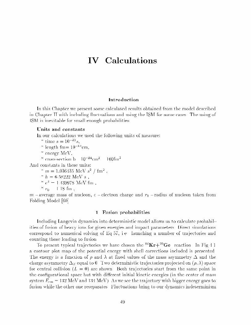
IV. CalculationsIntroductionIn this Chapter we present some calculated results obtained from the model describedin Chapter II with including uctuations and using the ISM for some cases. The using ofISM is inevitable for small enough probabilities.Units and constants.In our calculations we used the following units of measure:* time �s = 10�22s,* length fm= 10�13cm,* energy MeV,* cross-section b= 10�24cm2 = 100fm2.And constants in these units:* m = 1:036435 MeV �s2 / fm2 ,* �h = 6.58222 MeV �s ,* e2 = 1.439978 MeV fm ,* r0 = 1.18 fm ,m - average mass of nucleon, e - electron charge and r0 - radius of nucleon taken fromFolding Model [60]. 1. Fusion probabilitiesIncluding Langevin dynamics into deterministic model allows us to calculate probabil-ities of fusion of heavy ions for given energies and impact parameters. Direct simulationscorrespond to numerical solving of Eq.57, i.e. launching a number of trajectories andcounting those leading to fusion.To present typical trajectories we have chosen the 86Kr+70Ge reaction. In Fig.4.1a contour plot map of the potential energy with shell corrections included is presented.The energy is a function of � and � at �xed values of the mass asymmetry � and thecharge asymmetry �Z equal to 0. Two deterministic trajectories projected on (�; �) spacefor central collision (L = 0) are shown. Both trajectories start from the same point inthe con�gurational space but with di�erent initial kinetic energies (in the center of masssystem Ecm = 132 MeV and 134 MeV). As we see the trajectory with bigger energy goes tofusion while the other one reseparates. Fluctuations bring to our dynamics indeterminism49

50 IV. Calculationsin a sense that for the same initial conditions for a given reaction trajectories can eithergo to fusion or to reseparation. This is shown in Fig.4.2. Four trajectories with includedthermal uctuations start with the same kinetic energy (Ecm = 132 MeV) and one ofthem goes to fusion. One could say then that the probability of fusion would be in thiscase equal to 1=4, whereas in the deterministic calculations (Fig.4.1) it is exactly equalto 0.117111

10599

123

135 ρ

λ

636993

129

120

93

Fig 4.1 Two deterministic trajectories on the contour plot potential map for the 86Kr+70Gereaction. The potential energy is shown in MeV with respect to separated nuclei in (�; �)-space.The trajectories start with initial kinetic energy 132 and 134 MeV in the center of the mass system.In Chapter II we considered three types of uctuations: 1) thermal uctuations; 2)asymmetry uctuations; and 3) dissipative uctuations. To compare the in uence of thesetypes of uctuations we again take the same reaction 86Kr+70Ge and investigate prob-abilities for fusion separately for each type in the energy region near \extra-push". Threecurves of excitation function are presented in Fig.4.3. Dotted curve corresponds to theasymmetry, dashed one to the dissipative and solid one to the thermal uctuations. Fromthis �gure we learn that e�ects of asymmetry and dissipative uctuations are rather smallin comparison to thermal uctuations | the width of excitation function correspondingto thermal uctuations is much bigger than of the others.We have used the model for calculations of the near-threshold fusion probabilities forthe 86Kr+136Xe reaction studied recently at GSI Darmstadt by Christelle Stodel et al[104]. Cross sections for di�erent channels were measured for this system at the near-

1. Fusion probabilities 51threshold energies. From the combined compound-residue cross sections, the dependenceof the fusion probability on the excitation energy of the compound nucleus was deducedby the authors of Ref. [104], see Fig.4.4. The deduced fusion probability increases fromPfus � 2 � 10�4 at Ecm = 195 MeV to Pfus � 1 at Ecm = 230 MeV. This is an especiallyinteresting reaction from the point of view of shell e�ects as in both colliding nuclei thereare closed neutron shells. Therefore one can expect to see clearly the role of the shelle�ects in this case. And indeed in the deterministic calculations the value of the extra-push energy is equal to 224.2 MeV in calculations with shell e�ects included and 228.7 MeVin calculations without shells. This should be compared to experimental value of 224 MeV[106], the energy at which fusion probability drops down to 1=2. In our calculations weattempted to check whether the rise of the fusion probability, observed already at quitelow energies, can be explained in terms of the standard fusion dynamics with uctuationsdetermined by the dissipation- uctuation theorem. In Fig.4.4 results of our calculationsfor the 86Kr+136Xe reaction are compared with the experimental data. By using theimportance sampling method, we were able to carry out conclusive calculations even atthe lowest energies where the fusion probabilities drop down to few times 10�5, and thus toverify the near-threshold part of the excitation function. Results of the calculations showthat the observed near-threshold fusion probabilities in the 86Kr+136Xe reaction cannotbe explained with the standard fusion dynamics model based on one-body dissipation.Clearly, fusion extends to lower energies than expected by the theoretical calculations.Fig 4.2 Stochastic trajectories forthe 86Kr+70Ge reaction. Four trajectories withincluded thermal uctuations start with the samekinetic energy 132 MeV and one of them goes tofusion. Fig 4.3 The excitation functions for the86Kr+70Ge reaction for di�erent kind of uc-tuations. Dotted curve corresponds to the asym-metry, dashed one to the dissipative and solid oneto the thermal uctuations.On the other hand independent on dissipation it is very hard to understand, on thebasis of the present model, experimental excitation function extending to energies almost6 MeV lower than the saddle point position (Fig.4.4). If one would forget dissipation andcalculate the fusion probability as a probability of penetrating the saddle point barrierit would cut down this fusion probability by many orders of magnitude and the point at195 MeV would be out of the picture.

52 IV. Calculations195 200 205 210 215 220 225 230

Ecm (MeV)

10-52

510

-42

510

-32

510

-22

510

-12

510

0

P fus

Deduced from experimentCalculated

Sadd

le

Esh

ell

extr

a-

push

Eex

tra

-pu

sh

86Kr +

136Xe

222Th

*

Fig 4.4 The excitation functions for the86Kr+136Xe reaction. Fig 4.5 Dependance of the transmisson coe�-cient Tl on angular momentum reaction. The up-per curve is calculated for the colliding energyEcm = 190 MeV, and the lower one for 185 MeV.The dashed arrows show critical2. Cross sectionsThe total fusion cross section at the kinetic energy E can be written as a sum over allpartial waves: �E = ��2X(2l + 1)Tl = X d�(l)dl (152)where Tl is the transmission coe�cient through the fusion barrier with angular momentumL = �hl, and the spin distribution (partial fusion cross section with respect to the orbitalangular momentum) is de�ned asd�(l)=dl = ��2(2l + 1)Tl (153)Here � is the de Broglie wavelength:�2 = �h22�Ecm ; � = mA1A2A1 + A2 (154)In order to describe fusion of heavy ions well above the barrier, classical trajectory modelsincluding frictional forces but neglecting statistical uctuations have been frequently used,e.g. Ref. [101{103] One applies a sharp cut-o� model for the transmission coe�cientTl = ( 1; for l < l0;0; for l > l0; (155)i.e. fusion occurs for l < l0, and the fusion excitation function reads�E = ��2 l0Xl=0(2l + 1) = ��h2�E (l0(E) + 1)2: (156)

2. Cross sections 53This formula has been applied in calculating fusion excitation functions throughout theperiodic table with the surface friction model [102]. The critical l-value for fusion l0was determined for each center-of-mass energy E by solving dynamical equations withoutthe uctuating forces; i.e. in this approximation the mean trajectory determines thefusion cross section. Technically, l0 is determined by running trajectories for each energyby diminishing the initial l-value, starting with a large one, until a trajectory with aparticular l-value is captured behind the barrier.The corresponding spin distributions are of the triangular form:d�(l)dl = ( ��2(2l + 1); for l < l0;0; for l > l0: (157)If statistical uctuations are taken into account we obtain smooth dependence of thetransmission coe�cient (probability for fusion) Tl on angular momentum instead of thestep function in deterministic case, Eq.155. This is shown in Fig.4.5 for the 86Kr+104Rureaction . Two functions for energies 185 MeV and 190 MeV are presented; the dottedlines indicate values of l0 in the sharp cut-o� calculations without uctuations.Fig 4.6 The excitation functions for the the86Kr+70Ge reaction. The curve lying on the cir-cles represents the experimental data [105], andsquares show our calculations. The dashed linecorrespond to the excitation function obtained byclassical calculations without statistical uctua-tions (It goes to 0 in approaching to the extra-push). Fig 4.7 The excitation functions for the the86Kr+104Ru reaction. See the description forFig 4.6Two reactions 86Kr+70Ge and 86Kr+104Ru have been taken to calculate cross sec-tions. Experimental data for these reactions were obtained at GSI, Darmstadt [105]. InFigs. 4.6 and 4.7 there are shown excitation functions. Dashed lines represent excitationfunction corresponding to deterministic calculations, (Eq.156). It is obvious that these

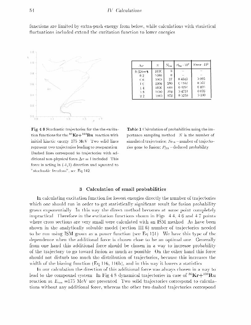
54 IV. Calculationsfunctions are limited by extra-push energy from below, while calculations with statistical uctuations included extend the excitation function to lower energies.Fig 4.8 Stochastic trajectories for the the excita-tion functions for the 86Kr+104Ru reaction withinitial kinetic energy 175 MeV. Two solid linesrepresent two trajectories leading to reseparation.Dashed lines correspond to trajectories with ad-ditional non-physical force �v = 1 included. Thisforce is acting in (-1,1) direction and squeezed to"stochastic freedom", see Eq.142.

�v N Nfus Pfus � 103 Error �1030 (Direct) 1000 0 - -0.2 1000 0 - -0.6 1000 37 0.4343 0.0951.0 1000 280 0.4347 0.0371.4 1000 696 0.4294 0.0241.8 1000 910 0.4731 0.0392.2 1000 973 0.5258 0.130Table 1 Calculation of probabilities using the im-portance sampling method. N is the number ofsimulated trajectories; Nfus - number of trajecto-ries gone to fusion; Pfus - deduced probability.3. Calculation of small probabilitiesIn calculating excitation function for lowest energies directly the number of trajectorieswhich one should run in order to get statistically signi�cant result for fusion probabilitygrows exponentially. In this way the direct method becomes at some point completelyimpractical. Therefore in the excitation functions shown in Figs. 4.4, 4.6 and 4.7 pointswhere cross sections are very small were calculated with an ISM method. As have beenshown in the analytically solvable model (section III.6) number of trajectories neededto be run using ISM grows as a power function (see Eq.151). We have this type of thedependence when the additional force is chosen close to be an optimal one. Generallyfrom one hand this additional force should be chosen in a way to increase probabilityof the trajectory to go toward fusion as much as possible. On the other hand this forceshould not disturb too much the distribution of trajectories, because this increases thewidth of the biasing function (Eq.116, 116b), and in this way it lowers a statistics.In our calculation the direction of this additional force was always chosen in a way tolead to the compound system. In Fig.4.8 dynamical trajectories in case of 86Kr+104Rureaction at Ecm =175 MeV are presented. Two solid trajectories correspond to calcula-tions without any additional force, whereas the other two dashed trajectories correspond

3. Calculation of small probabilities 55to calculations with an additional force �v = 1. In this way one can see how adding an ad-ditional force is changing the dynamical behaviour of the system going from reseparationto fusion.In Table 1 results of the fusion probability for the same case as in Fig.4.8 as a functionof the amplitude of the additional force is presented. One can see that in the region of�v = (0:6; 1:4) we obtain stable results for the fusion probability with error bars beingthe lowest for �v = 1:4. In this way one could say that the value �v = 1:4 is an optimalone in this case.

V. Summary and conclusionsWe have shown how one can introduce uctuations into a deterministic descriptionof Heavy Ion Dynamics. This is absolutely unavoidable in case one wants to reproduceexperimentally observed distributions and not only their average values.Chapter II is devoted to the description of the deterministic model of Heavy Ion Col-lisions with stochastic e�ects included. It consists of two parts: in the �rst one we havedescribed deterministic model of HIC, and in the second one we elaborated statistical uctuations. A Langevin description of HI dynamics, suitable for implementation in nu-merical simulations, is easily derived. This approach can be studied by starting with adeterministic model of HI collisions, then adding the stochastic forces, and �nally simu-lating the resulting dynamics numerically. From these simulations one is able to obtainan excitation functions for fusion { experimentally observed quantities, which can thenbe compared directly with experimental data.The derivation of Langevin description of nuclear dynamics is not the end of thestory. Statistical uctuations play an important role speci�cally in process for which theinteresting outcome { e.g. fusion of heavy elements { occurs with very low probability.In such situations, direct numerical simulations of the process do not provide a realisticmethod of attacking the problem.In connection to that in Chapter III there are presented new methods we have devel-oped of getting around this problem obtaining very encouraging results. One approachmakes use of a one-to-one correspondence between the statistical distributions of Langevintrajectories, and the thermal distributions of directed polymers. This analogy provides apowerful formalism for analyzing relative probabilities of Langevin trajectories. We havetested this method on both simple schematic but analytically solvable model, and thesimpli�ed model of HIC [2]. This method has turned out to be very powerful in a sensethat the calculational e�ort does not depend on how small are the probabilities we wantto calculate. However it demands a big number of sampling. And we did not use it forcalculations with a realistic model as due to the complicated dynamics of this model theprocess of sampling takes a lot of the computer time.The other method (called by us ISM) involves adding, in our numerical Langevin sim-ulations, an extra, non-physical force acting on the nuclear collective degrees of freedom.This force is chosen so as to increase the probability for fusion by orders of magnitude,enabling us to obtain good statistics from a reasonable number of simulations; then weanalytically correct for the inclusion of this unphysical force, thus �nally obtaining thedesired cross section. We have tested �rst this method in di�erent models and have ob-56

Summary and conclusions 57tained fusion probabilities in situations where they are extremely small. We have foundthat we could get good statistics with far fewer simulations that is needed to accuratelyextract the fusion probability by direct Langevin simulation. We were encouraged by theresults we obtained from simpli�ed model of nuclear collisions. So we used this methodto calculate probabilities (cross sections) within more realistic model.Results of the calculations for three di�erent reactions: 86Kr+104Ru, 86Kr+70Geand 86Kr+136Xe are presented in Chapter IV. Comparison with an experimental datashows that the model is working properly in the region of high probabilities of fusion butis falling down too fast for the subbarrier region.In here we have presented ideas one can follow in many �elds. As far as the processof fusion is concerned it is possible now to try to make estimates for the cross sections inthe exotic superheavy region.We have shown how one can introduce uctuations into a deterministic description ofheavy ion dynamics. At the same time we have proposed methods for calculating smallprobability events within a reasonable statistics and not too much of the computationale�ort. Those methods are quite general and can be applied not only in nuclear physics butalso in other �elds of physics where one is dealing with a very small but still measurablecross sections.

VI. Appendix: Solvable modelsAt the time we were developing a model of nuclear dynamics with uctuations someproblem appeared which are not directly related to nuclear physics but strictly speakingto statistical physics. The description of those problems was added to this thesis.1. IntroductionIn this chapter we present three di�erent models. The �rst is Feynman's ratchet andpawl discrete simpli�ed model. It operates between two heat reservoirs. We solve exactlyfor the steady-state directed motion and heat ows produced, �rst in the absence andthen in the presence of an external load. We show that the model can act both as aheat engine and as a refrigerator. We �nally investigate the behavior of the system nearequilibrium, and use our model to con�rm general predictions based on linear responsetheory.In recent years, a number of theoretical results pertaining to systems far from thermalequilibrium have been derived. While not identical to one another, these results beara similar structure, and the term uctuation theorem (FT) has come to refer to themcollectively. The rest two highly idealized, but exactly solvable, models are shown mainlyfor applying the uctuation theorem. One involves a piston inside an in�nite cylinder,surrounded by two ideal gases at di�erent temperatures. The other involves a particledragged through a thermal environment by a uniformly translating harmonic force. Forthese models we are interested in the entropy production distribution function. We showthat the solutions satisfy the relations of the uctuation theorem.2. Feynman's ratchet and pawlIntroduction. Feynman's ratchet and pawl system [70] is a well known (but notthe earliest! [71]) example of a proposed \mechanical Maxwell's demon", a device whosepurpose is to convert into useful work the thermal motions present in a heat reservoir.The idea is beautifully simple: set up a ratchet and pawl so that a wheel is allowed toturn only in one direction, and then attach that wheel to a windmill whose vanes aresurrounded by a gas at a �nite temperature; see Fig.46-1 of Ref. [70]. Every so often,an accumulation of collisions of the gas molecules against the vanes will cause the wheelto rotate by one notch in the allowed direction, but presumably never in the forbiddendirection. Such recti�cation of thermal noise could be harnessed to perform useful work58

2. Feynman's ratchet and pawl 59(such as lifting an ea against gravity), in direct violation of the Second Law. Of course,in order for statistical uctuations to cause rotation at a perceptible rate, the ratchet andpawl must be microscopic, and this points to the resolution of the paradox. If thermalmotions of the gas molecules are su�cient to cause the wheel to rotate a notch, then thethermal motion of the pawl itself will occasionally cause it to disengage from the ratchet,at which point the wheel could move in the \forbidden" direction. Feynman comparedthe rates of the two processes { rotation in the allowed and the forbidden directions { andfound them to be equal when the system is maintained at a single temperature. Thus nonet rotation arises, and the Second Law is saved.Since the failure of the ratchet and pawl system to perform work arises from thermal uctuations of the pawl, a natural solution to the problem is to reduce these uctuationsby externally cooling the pawl to a temperature below that of the gas. In this case thedevice does indeed operate as designed, but this no longer constitutes a violation of theSecond Law: the ratchet and pawl is now e�ectively a microscopic heat engine, capitalizingon a temperature di�erence to extract useful work from thermal motions.While the ratchet and pawl was introduced in Feynman's Lectures primarily for peda-gogical purposes, recent years have seen a renewed interest in this system [72{86], largelydue to the fact that analogous mechanisms have been proposed as simple models of motorproteins.Our purpose in this section is to introduce an exactly solvable model of Feynman'smicroscopic heat engine. This model is discrete rather than continuous16, but it capturestwo essential features of the original example: (1) a periodic but asymmetric interactionpotential between the ratchet and the pawl (corresponding to an asymmetric sawtoothshape for the ratchet's teeth), and (2) two \modes" of interaction (corresponding to thepawl being either engaged or disengaged from the ratchet). These features are su�cientfor the model to reproduce the behavior discussed by Feynman. A di�erent discrete modelof noise-induced transport has been studied by Schimansky-Geier, Kschischo, and Fricke[84]; however, we believe ours to be the �rst in which (as in Feynman's example) thetransport is explicitly driven by a temperature di�erence between two reservoirs.Zero external load. We begin this section by introducing our model in theabsence of an external load, then pointing out the analogy with Feynman's ratchet andpawl. Following that, we solve the model.Consider a particle which moves via discrete jumps between neighboring sites along aone-dimensional regular lattice, where d is the lattice spacing. We assume that the particleis coupled to a heat reservoir at temperature TB, and that its jumps are thermal in nature.That is, the probability (per unit time) of making a jump to site i+ 1, starting from sitei, is related to the probability rate of the inverse process by the usual detailed balancerelation: Pi!i+1=Pi+1!i = exp(��E=TB), where �E = U (m)i+1 � U (m)i is the instantaneouschange in the particle's potential energy, associated with the jump from i to i+1. We use16Note that a particle (or, more generally, a reaction coordinate), evolving from one su�cientlydeep potential (or free) energy minimum to another, behaves much as if hopping from one siteto another on a discrete lattice. See, for instance, Fig.6 of Ref. [83].

60 VI. Solvable models of stochastic behaviorthe notation U (m)i to denote the potential energy of the particle at site i; the superscriptm denotes the \mode" of the potential, to be explained momentarily. The integer indexi runs from �1 to +1, and we are using units in which Boltzmann's constant kB = 1.Mode 1 Mode 2

−α

+α

0

i=1

d

Fig A.1 The potential energy U (m)i is shown forboth modes, m = 1; 2, in the absence of an ex-ternal load; the lattice spacing is d, and site 1 islabeled explicitly.S W

T

T

A

B

QB

QAFig A.2 A schematic representation of our sys-tem (S) in contact with two heat reservoirs (attemperatures TA and TB). As implied by the ar-rows, we de�ne _QA to be the net ow of heat fromreservoir A to the system, and _QB to be the heat ow from the system to reservoir B. Therefore_W = _QA � _QB is the power delivered as workagainst an external load. (First we consider thatthere is no such load, hence _QA = _QB.)Next, we assume that the potential energy function U (m)i has two possible modes,m = 1; 2, and that it changes stochastically between these two. In the �rst mode, thepotential energy of each site is zero: U (1)i = 0. In the second mode, the potential energy isperiodic, with period 3: U (2)i = � �[(i mod 3)�1], where � is a positive constant with unitsof energy. As shown in Fig.A.1, the second mode is a discrete version of an asymmetricsawtooth potential. We assume that the stochastic process governing the changes betweenmodes is also a thermal process, driven by a heat reservoir at temperature TA. Thus, theprobability rate of a change to mode 2, starting from mode 1, relative to the probabilityrate of the reverse mode change, is given by the detailed balance factor exp(��E=TA),where �E = U (2)i � U (1)i is now the (site-dependent) change in particle energy due to aninstantaneous change from mode 1 to mode 2.We now describe more precisely these two stochastic processes, the one governing thejumps of the particle, the other governing the change between modes. First, we assumethat the processes are independent of one another, and that each is a Poisson processoccurring at a rate �. That is, during every in�nitesimal time interval �t, there is aprobability ��t that the particle will attempt a jump to a neighboring site. An \attempt"looks as follows. First, the particle decides (randomly, with equal probability) whetherto try jumping to the left (�d) or to the right (+d). Then the Metropolis algorithm[87] is used to satisfy detailed balance: if the value of �E associated with the jump

2. Feynman's ratchet and pawl 61is zero or negative, then the jump takes place; if �E > 0, then the jump occurs withprobability exp(��E=TB). Similarly, during every in�nitesimal time interval �t, thereis a probability ��t that the mode will attempt to change. Again, the attempt is eitheraccepted or rejected according to the Metropolis algorithm (at temperature TA).We have introduced three parameters which we will view as being \internal" to thesystem: d, �, and �; these essentially set the length (d), energy (�), and time (��1) scalesrelevant for the system. The two remaining parameters entering the model, TA and TB,we will view as \external".The analogy between our model and Feynman's ratchet and pawl runs as follows. First,the position of our particle corresponds to an angle variable, �, specifying the orientationof the ratchet wheel. When the particle accomplishes a net displacement of three latticesites, either to the right or to the left, this is equivalent to the ratchet being displaced byone notch, or tooth17; see Fig.A.1. Since we want to keep track of the wheel over longintervals of time, possibly including many full rotations, � varies from �1 to +1, ratherthan being a periodic variable from 0 to 2�; this is why the variable i, specifying thelattice site, takes on all integer values.When a ratchet and pawl are \engaged" { that is, when the pawl actually pressesagainst the teeth of the ratchet { then there exists an interaction energy, arising from thecompression of the spring which holds the pawl against the ratchet, which has the form ofa periodic sawtooth potential in the angle variable �. In our discrete model, the analogueof this interaction energy is the discrete sawtooth potential U (2)i described above; mode2 thus corresponds to the situation in which the ratchet presses against the pawl. Bycontrast, mode 1 corresponds to the ratchet and pawl begin \disengaged", as will occurevery so often as a result of thermal uctuations of the pawl. Of course, in Feynman'ssystem, the potential energy of the disengaged mode is always greater than that of theengaged mode (due to the spring compression needed to actually place the pawl out ofreach of the ratchet's teeth), whereas in our model this is not the case: U (1)i = 0. This,however, does not change the problem in any qualitatively signi�cant way.As mentioned, the motion of the particle from site to site is a thermal process occurringat temperature TB, while the stochastic \ ashing" between modes 1 and 2 is a thermalprocess occurring at temperature TA. Thus, in the context of the analogy with the physicalratchet and pawl, TB denotes the temperature of the gas surrounding the panes connectedto the ratchet wheel, and TA is the temperature at which the pawl is maintained.Given this model, we would like to know whether a current arises: in the long run,will there be a net drift of the particle { corresponding to a non-zero angular velocity ofthe wheel in the original ratchet and pawl { and if so, what will be the rate and directionof the drift?Our system of two coupled spins has six possible states, which we number with anindex n,1 2 3 1

4654 . The dynamics of the particle is described by stochastic jumps amongthese six states. This is a Markov process, and we can describe its statistics with a set17Thus, the distance 3d in our model translates to an angular interval �� = 2�=Nteeth, whereNteeth is the number of teeth along the perimeter of the ratchet wheel.

62 VI. Solvable models of stochastic behaviorof rate equations. Let pn(t) denote the probability that the system is found in state nat time t. Then the evolution of these probabilities is governed by the following set ofcoupled equations:dpndt = � Xn0 6=n�pn0P (n0 ! n)� pnP (n! n0)� ; n = 1; � � � ; 6: (158)Here, � �P (n! n0) is the probability rate at which the system, when its state is n, makesa transition to state n0.Our rate equations can be expressed as:dpdt = �Rp; (159)where p = (p1; � � � ; p6)T , R is the 6� 6 matrixR = 0BBBBBBBBBBB@ �2 12 12 � 0 012 �2 12 0 1 012 12 �1� � 0 0 11 0 0 ��� �+�22 12 120 1 0 �2 �3+�2 120 0 � �22 �2 �2 1CCCCCCCCCCCA ; (160)and we have introduced the constants� = e��=TA and � = e��=TB: (161)Note that � and � are monotonically increasing functions of TA and TB, and the temper-ature range 0 < TA (TB) < 1 translates to 0 < � (�) < 1. We thus think of � and � is\rescaled" temperatures.As a consistency check, note that the elements in each column of R add to zero:PmRmn = 0. Thus, R annihilates the row vector 1T = (1; 1; 1; 1; 1; 1) by left multiplica-tion: 1TR = 0T , which means that total probability is conserved:ddtXn pn = ddt(1T � p) = 1T � (�Rp) = 0: (162)The long-time behavior of our system is governed by the steady-state distribution ofprobabilities, �p, which is the null eigenvector of R:R�p = 0: (163)Determining �p is a straightforward exercise in Jordan elimination, and leads to the fol-lowing result: �p = x=N , where

2. Feynman's ratchet and pawl 63x1 = 52� + 28�2 + 12� + 19�2 + 5�3 + 21�� + 2��2 + 8�2� (164)x2 = 36� + 16�2 + 28� + 27�2 + 5�3 + 25�� + 8��2 + 2�2� (165)x3 = 44� + 19�� + 20� + 49�2 + 15�3 (166)x4 = 64 + 20� + 48� + 15�� (167)x5 = 24� + 40� + 20�2 + 18�2 + 30�� + 15��2 (168)x6 = 22�2 + 16�� + 44��2 + 14�2� + 15��3 + 26�2 + 10�3; (169)and N(�; �) = P6i=1 xi is a normalization factor.When both temperatures go to zero, �; � ! 0, we get �pT = (0; 0; 0; 1; 0; 0). This makessense: in that limit, the system freezes to the state of lowest energy, which is state 4.We now address the question of net drift. We �rst de�ne a net current, J � J+ � J�,where J+ is the rate at which particle drift from states 2 and 5 to 3 and 6, and J� isthe rate of the reverse transitions. By \rate", we mean number of passes per unit time,averaged over an in�nitely long interval of time. The current J represents the net averagerate of particle drift. In the length units:v = 3 dJ; (170)where v denotes the (steady-state) average velocity of the particle.Explicit expression for the quantities J� are given by:J+ = � (�p2R32 + �p5R65) (171)J� = � (�p3R23 + �p6R56): (172)(Recall that �Rmn is the transition rate to state m, given that the system is found instate n; therefore �pn�Rmn is the net rate at which transitions from n to m are observedto occur in the steady state.) Using our results for �p, we compute J�, take the di�erenceto get J , and �nally multiply by 3 d to get, after some algebra:v(TA; TB) = �3 d �N (�� �)(1� �)(3� + 4): (173)There are a number of things to note about this result. First, it implies that if TA > TB(i.e. � > �), then there is a net ow of the particle to the left; if TB > TA, the particledrifts to the right. If the temperatures are equal, then there is no drift, in agreement withFeynman's analysis (as well as the Second Law!).Next, notice that v ! 0 as TB ! 1 (� ! 1). In that limit, the change in energyarising from a jump to the left or to the right becomes negligible in comparison to thetemperature of the reservoir which drives those jumps; thus, from any lattice site, theparticle is as likely to jump to the left as to the right, resulting in no net drift.Finally, in the limit TA !1 (�! 1), we get:v = �21 d �N (1 � �)2 ; TA !1: (174)This is the limit in which changes between the modes occur independently of locationof the particle: every attempt to change the mode is accepted. This is analogous to the

64 VI. Solvable models of stochastic behaviorsituation studied by Astumian and Bier [73], where the \ ashing" between the two modesof the potential is simply a Poisson process at a �xed rate, independent of the particleposition..004

-.03

0.0.001

-.001

-.015

-.005

v=.01

ν

µ0.0 0.5 1.0

1.0

0.0

0.5Fig A.3 A contour plot of the function v(�; �),where � = exp(��=TA) and � = exp(��=TB) arethe rescaled temperatures of the two reservoirs.= 1/2

S.

10 v

.Q BA

ν

µ

Fig A.4 The drift v (multiplied by 10), heat ow_QA!B, and rate of entropy production _S, plottedas functions of �, for �xed � = 1=2.We can also use our expression for the steady-state probability distribution to computethe average rate at which heat is transferred between the two reservoirs and our system.Whenever the system makes a transition from state 1 to state 4, or from state 6 to state3, its energy drops by �; this energy is released into the reservoir coupled to spin A (attemperature TA). Conversely, during the transitions 4 ! 1 and 3 ! 6, the system absorbsenergy � from reservoir A. Since no other transitions involve a transfer of energy betweenthat reservoir and the system, we can express the net rate at which the system absorbsenergy from reservoir A as:_QA = �� ��p4R14 + �p3R63 � �p1R41 � �p6R36�: (175)We can similarly write down an expression for _QB, the rate at which heat ows from oursystem to reservoir B:_QB = �� ��p5R45 + �p6R56 + 2�p6R46 � �p4R54 � �p5R65 � 2�p4R64): (176)Fig.A.2 illustrates the sign convention which we choose in de�ning _QA and _QB. Afterplugging in the values for the components of �p and R, we �nd that _QA = _QB, as we couldhave predicted, since in the steady state there is no net absorption of heat by the system,nor is any of the heat delivered as work against an external load. Thus, the particle driftis ultimately driven by a net passage of heat from A to B, by way of the system. Theexplicit expression for this heat ow is given by:_QA!B = _QA = _QB = 3 ��N (� � �)P (�; �); (177)where P (�; �) = 4 + 14� + 15� + 4�� + 5�2 > 0.

2. Feynman's ratchet and pawl 65The factor (� � �) in Eq.177 guarantees that the direction of the heat ow is fromthe hotter to the cooler reservoir (or not at all if TA = TB). Since the same factorappears in Eq.173, and since all other factors in these equations are positive, these twoequations show explicitly that the direction of the ow of heat determines the directionof the particle motion: when the heat ows from A to B, the particle drifts to the left;when it ows from B to A, the particle drifts rightward. The ratio v= _QA!B then givesus the average displacement of the particle, per unit of heat passed (via the system) fromreservoir A to reservoir B:lim�!1 �x�Q = v_QA!B = � d� � (1 � �)(3� + 4)P (�; �) < 0: (178)Here, �x and �Q are the net particle displacement, and the net heat transferred from Ato B, respectively, over a time interval � .We can also compute the rate at which entropy is produced during this process. Therate of entropy production associated with the ow of heat from reservoir A to the systemis: _SA = � _QA=TA; and for reservoir B: _SB = _QB=TB. The net entropy production rateis thus: _S = _SA + _SB = TA � TBTATB _QA!B (179)= 3 �N �ln ��� (�� �)P (�; �) � 0: (180)Figs.A.3 and A.4 illustrate the results obtained in this subsection. Fig.A.3 is a contourplot of the drift v, as a function of the rescaled reservoir temperatures � and �. Thecontour v = 0 runs along the diagonal, � = �, as well as along � = 1 (TB ! 1). Theappearance of positive contours (v > 0) to the left of the diagonal, and negative onesto the right, illustrates the point that the drift is rightward when TB > TA and leftwardwhen TA > TB.In Fig.A.4 we have �xed the value of TA by setting � = 1=2, and have plotted v,_QA!B, and _S as functions of �. All three quantities hit zero at � = 1=2, where TA = TB:nothing interesting happens when the system is maintained at a single temperature. Notealso that v and _QA!B are opposite in sign (in agreement with Eq.178), while _S is alwaysnonnegative (in agreement with the Second Law). Finally, note that v ! 0 as � ! 1(TB !1).In plotting these two �gures, we set all the internal parameters to unity: � = d = � =1. Nonzero external load. In this subsection we add an external load to our simplemodel. In Feynman's example, this load is an ea, attached by a thread to the ratchetwheel: when the wheel rotates in the appropriate direction, the creature is lifted againstgravity. In our model, we add a slope to the discrete potential:U (m)i ! U (m)i + ifd; (181)where f is a real constant (and i is still the lattice site variable, not p�1). E�ectively, fis a constant external force which pulls the particle leftward if f > 0, rightward if f < 0.

66 VI. Solvable models of stochastic behaviorThe presence of an external load allows the system to perform work. If, in the steadystate achieved for �xed x = (f; TA; TB), the particle experiences a drift v(x), then thepower (work per unit time) delivered against the external load is:_W (x) = fv(x): (182)By conservation of energy, this must be balanced by heat lost by the reservoirs:_W = _QA � _QB: (183)Our approach to solving for the steady-state behavior is the same as in the previoussubection. We are interested in the quantities v(x), _QA(x), and _QB(x) which describethat behavior. As before, we map our model onto a two-spin, six-state system, whosestatistical evolution is governed by the rate equations dp=dt = �Rp (Eq.159). There isthen an associated steady state �p, and the quantities in which we are interested are given,as in the previous subection, by:v = 3 d���p2R32 + �p5R65 � �p3R23 � �p6R56� (184a)_QA = �� ��p4R14 + �p3R63 � �p1R41 � �p6R36� (184b)_QB = �� ��p5R45 + �p6R56 + 2�p6R46 � �p4R54 � �p5R65 � 2�p4R64): (184c)The only di�erence is that the presence of the term ifd in the potential changes theelements of R, and therefore the vector of steady-state probabilities �p.Because the acceptance probability of an attempted move in the Metropolis schemehas the form Prob: = minf1; exp��E=Tg, there is no general analytic expression for thematrix R valid for all values of f . Instead, the elements of R are piecewise analytic inf ; the analytic expression for Rij depends on the sign of the transition energy �Ej!i. Alittle thought reveals that the f -axis can be divided into four ranges of values, over eachof which the elements of R can be written as analytic functions of �, d, f , TA, and TB.These ranges are: �1 < f< ��=d (185a)��=d < f< 0 (185b)0 < f< 2�=d (185c)2�=d < f< +1: (185d)In the two extreme ranges, (a) and (d), stretching to �1 and +1, the slope is so steepthat the potential energy function no longer has a sawtooth shape in mode 2. We willignore these ranges and focus instead on the ones for which U (2)i does look like a discretesawtooth.For range (b), i.e. ��=d < f < 0, the potential slopes downward with increasing i,and an explicit expression for R is:

2. Feynman's ratchet and pawl 67Rb = 0BBBBBBBBBBB@ �32 � 12� 12� 12 � 0 012 �32 � 12� 12� 0 1 012� 12 �12 � � � 12� 0 0 11 0 0 �� � �22� � ��2 12 120 1 0 ��2 �32 � ��2 120 0 � �22� ��2 �2 1CCCCCCCCCCCA ; (186)where � = e�fd=TB : (187)For range (c), 0 � f < 2�=d, the potential slopes upward with i, and we haveRc = 0BBBBBBBBBBB@ �32 � �2 12 �2 � 0 0�2 �32 � �2 12 0 1 012 �2 �12 � �� �2 0 0 11 0 0 ��� �22� � ��2 12 120 1 0 ��2 �32 � ��2 120 0 � �22� ��2 �2 1CCCCCCCCCCCA : (188)Note that both Rb and Rc reduce to the matrix R of the previous subection, when � = 1,i.e. f = 0.As in the previous subection, the �rst order of business is to solve for the steady-statedistribution of probabilities, �p. This is again an exercise in Jordan elimination, only nowthe process is considerably more tedious: terms do not cancel as nicely as when f = 0.The �nal results for the steady state probabilitie vectors �pb and �pc (corresponding to thetwo ranges of f values) are of the form�pjn = P jn(�; �; �)N j(�; �; �) ; j = b; c; n = 1 � � � 6; (189)where the P jn's are �nite polynomials in the variables �, �, and �, and N j = P6n=1 P jn isa normalization factor. Explicit expression for the polynomials P jn are given in the lastsubsection of this section.We can now use Eq.184 to obtain v(x), _QA(x), and _QB(x). The results for the tworanges of f values, j = b; c, are:vj(x) = 32d� Xj�N j_QjA(x) = �� Y jN j_QjB(x) = �� Y jN j � 32fd� Xj�N j ; (190a)(190b)(190c)

68 VI. Solvable models of stochastic behaviorwhere Xj(�; �; �) and Y j(�; �; �) are polynomials for which explicit expressions are pre-sented in the last subsection of this section.Note that the steady-state behavior described by Eq.190 clearly satis�es energy con-servation (see Eqs.182 and 183): _QA � _QB = fv: (191)Since v, _QA, and _QB are not independent (i.e. they satisfy the above relation), the \spaceof steady-state behaviors" is e�ectively two-dimensional.Eq.190 is the central result of this section. For arbitrary temperatures TA and TB,and for any external load f such that the interaction potential retains its sawtooth shape(��=d < f < 2�=d), Eq.190 gives the directed motion and heat ows which describe thesteady-state behavior of the system for those external parameter values. These resultsreduce to those of the previous subection when we set f = 0. In the next subsection,we use the above results to show that our model can act both as a heat engine and asa refrigerator. In the following subsection, we consider the behavior of our system nearequilibrium, and we use Eq.190 to con�rm predictions based on a general, linear responseanalysis.γ

f

v=0

β=1

Fig A.5 The contour v(f; ) = 0 is shown, for�xed average inverse temperature � = 1. Theshaded regions are those for which fv > 0, i.e.for which the system behaves as a heat engine.γ

f

A

.Q = 0

.Q = 0B

β=1

Fig A.6 The contours _QA(f; ) = 0 and_QB(f; ) = 0 are shown, for �xed � = 1. Inthe shaded regions, there is a net ow of heat outof the colder reservoir; the system then acts as arefrigerator.The system as heat engine and refrigerator. We can anticipate two di�erentscenarios in which our system acts as a \useful" device:(1) _W > 0. In this case, the system is a heat engine, causing the particle to drift upthe potential energy slope, with e�ciency �eng = _W= _Q>, where _Q> is the rate of heat ow out of the hotter reservoir.(2) _W < 0 and _Q< > 0, where _Q< is the rate of heat ow out of the colder reservoir.Here the system is a refrigerator, with e�ciency �ref = _Q<=j _W j. The particle drifts downthe potential slope, and the resulting energy liberated allows for a net transfer of heatfrom the colder to the hotter reservoir, without violating the Second Law.

2. Feynman's ratchet and pawl 69We will now use the results derived in the previous subsection to show that our simplemodel indeed exhibits both these behaviors.The system is a heat engine when v(f; TA; TB) and f are of the same sign; see Eq.182.To demonstrate that our model exhibits this behavior, let us introduce the variables� = TA + TB2TATB (192) = TA � TBTATB ; (193)and consider the behavior of our system in (f; )-space, for a �xed value of �. Thatis, we hold �xed the average inverse temperature of the reservoirs (�), and consider theoperation of the system in terms of the external load (f) and the di�erence betweeninverse temperatures of the reservoirs ( ). (We will use these variables again in thefollowing subsection. Furthermore, because _QA, _QB, and v are mutually dependent { seeEq.191 and the comment following it { we can generically explore a measurable fractionof the two-dimensional space of steady-state behaviors by varying only two independentexternal parameters, f and , while holding the third, �, �xed.)In Fig.A.5 we plot the contour v(f; ) = 0, having set � = 1, and with the internalparameter values � = d = � = 1. (The range of values for this choice of � is �2 < <2.) To the left of this contour, we have v > 0; to the right, v < 0. The shaded regionthus represents the values of (f; ) for which v and f are of the same sign, i.e. where thesystem behaves as a heat engine.We can understand the placement of the shaded region as follows. Consider a point Pon the positive -axis: f = 0, > 0. This corresponds to TA > TB, with no external load.We know that the particle then drifts leftward, v < 0, although no work is performed,since f = 0. Let us now imagine that we tilt the potential slightly \downward" (f < 0).For a small enough tilt, we expect that the particle will continue to drift to the left, butnow this drift is uphill, and therefore work is done against the external load: _W > 0. Weconclude that points immediately to the left of the positive vertical axis will correspondto external parameters for which the system behaves as a heat engine. Fig.A.5 con�rmsthis: the shaded region hugs the positive -axis from the left. (Similar reasoning appliesfor the negative -axis, where the region _W > 0 appears to the right.) If we now continueto tilt the slope more and more downward (f increasingly negative), at �xed > 0, weexpect the leftward drift to become progressively slower, until for some tilt we get v = 0.At this point the leftward \thermal force" exerted on the particle due to the temperaturedi�erence between the reservoirs, exactly balances the external load. This occurs at theboundary of the shaded region (the contour v = 0): for more negative slopes, the particleslides down the slope, and the system no longer acts as a heat engine.Our system is a refrigerator when _Q< > 0, where _Q< is the rate at which heat leavesthe colder of the two reservoirs. In Fig.A.6 we plot the contours _QA(f; ) = 0 and_QB(f; ) = 0, again for � = 1. These two contours are tangent at the origin, and dividethe plane of (f; )-values as follows: _QA > 0 for points lying above the contour _QA = 0,and _QA < 0 for points lying below that contour. Similary, _QB > 0 ( _QB < 0) for pointslying above (below) the contour _QB = 0. Now, above the horizontal axis ( > 0) we haveTA > TB, hence _Q< = � _QB. The small shaded region in the second quadrant therefore

70 VI. Solvable models of stochastic behaviorrepresents values of (f; ) for which reservoir B is the colder of the two reservoirs, andit is losing heat (since _QB < 0). Hence in this region our system acts as a refrigerator.Below the horizontal axis, TB > TA and thus _Q< = _QA. The larger shaded region inthe fourth quadrant thus also represents refrigeration, only now reservoir A is the beingdrained of heat.We can understand the general shape of the shaded regions by assuming that, whenthe temperatures are equal ( = 0) and the slope is very small, the quantities v, _QA, and_QB are linear functions of the slope:v(f; 0) = cvf + O(f2) (194a)_QA(f; 0) = cAf + O(f2) (194b)_QB(f; 0) = cBf + O(f2); (194c)with cv; cA; cB 6= 0. (Then cv < 0, since the particle cannot slide up the slope whenthe reservoir temperatures are equal.) Energy conservation implies that the di�erencebetween _QA and _QB must be quadratic in f (since _QA � _QB = _W = fv = cvf2), hencecA = cB: (195)Thus, for equal temperatures and a su�ciently small slope, one of the reservoirs will belosing heat and the other will be gaining it. If we now slightly lower the temperature ofthe reservoir which is losing heat, then we have a refrigerator: heat ows out of the colderreservoir. In our model, we have c � cA = cB > 0, hence for points on the = 0 axisimmediately to the right of the origin, heat ows out of reservoir A and into reservoir B;immediately to the left of the origin the reverse holds true. This explains why, just tothe right (left) of the origin, the shaded region corresponding to refrigeration hugs thehorizontal axis from below (above). If we continue to the right along the line = 0,increasing the value of f , then the particle will drift ever more rapidly to the left as theslope becomes ever more steeply inclined. The potential energy lost as the particle slidesdown the incline gets dissipated into the reservoirs; for su�ciently large f , the rate ofdissipation is great enough that both reservoirs become heated: _QA < 0, _QB > 0. Thishappens to the right of the point at which the contour _QA = 0 crosses the horizontal axiswith a positive slope; for values of f beyond this point the system can no longer operateas a refrigerator.We can also understand why the two contours _QA = 0 and _QB = 0 \kiss" at theorigin. The result cA = cB means that _QA and _QB are (to leading order) equal along thehorizontal axis = 0, near the origin. However, they are also (exactly) equal along thevertical axis, since _W = 0 when f = 0. Thus, _QA and _QB are equal, to leading order in fand , for a small region around the origin: _QA = _QB = cf + b . This implies that theircontours are both tangent to the line = �cf=b at the origin.Since we have explicit expressions for v(x), _QA(x), and _QB(x), we can analyticallycompute the thermal e�ciency � associated with the steady-state operation of our model,when it acts as either a heat engine or a refrigerator. By the Second Law, these e�cienciesmust never exceed the Carnot e�ciencies, �Ceng and �Cref (which depend only on TA andTB). Ideally, we could use our exact results to �nd the maximum relative e�ciency(y = �=�C) which our model achieves, both when it acts as a heat engine and when it

2. Feynman's ratchet and pawl 71acts as a refrigerator. Unfortunately, the expressions for v, _QA, and _QB are su�cientlycomplicated (see the last subsection of this section) that we are not able to �nd thesemaxima analytically. However, at the end of the next subsection, we will present analyticalresults for the maximum relative e�ciencies achieved when the system operates close toequilibrium.Linear Response. When there is no external load and the reservoir temperaturesare equal (TA = TB = ��1), our system is in thermal equilibrium, and there results noaverage particle drift or heat ow: v = _QA = _QB = 0. In the previous subsection webrie y considered the behavior of our system near equilibrium (see e.g. Eq.194). We nowconsider this case in more detail. We will present a general analysis essentially the sameas that of J�ulicher, Ajdari, and Prost [81], and then we will show that the exact resultsobtained for our model con�rm the predictions of this analysis.For a su�ciently small load f and inverse temperature di�erence , and a �xed valueof � (characterizing the inverse temperature of the equilibrium state around which weexpand), we expect to be in the linear response regime: the particle drift and heat owsdepend linearly on f and . Let us introduce the quantity� = 12� _QA + _QB� (196){ roughly, a \heat ux" from A to B { and let us write, to leading order in f , : v� ! = @v=@f @v=@ @�=@f @�=@ ! f ! ; (197)with the derivatives of v and � { re-expressed as functions of (f; ; �) rather than(f; TA; TB) { evaluated at equilibrium (f = = 0). As per the arguments given atthe end of the previous subsection, _QA and _QB are equal, to leading order in f and ,near equilibrium.The rate of entropy production is then:_S = � _QATA + _QBTB= �� _W + �= (f ) M11 M12M21 M22 ! f ! ; (198)where M11 = �� @v=@f , M12 = �� @v=@ , M21 = @�=@f , and M22 = @�=@ , evaluatedat equilibrium. The Second Law implies thatdetM � 0; (199)whereas Onsager's reciprocity relation [88] predicts that M12 = M21, or� �@v@ !eq = @�@f !eq: (200)

72 VI. Solvable models of stochastic behaviorAlso, the diagonal elements of M must be positive: the particle must slide down thepotential slope when the temperatures are equal (M11 > 0), and there must be a ow ofheat from the hotter to the colder reservoir when the slope is zero (M22 > 0). J�ulicheret al. [81] have obtained identical results for a molecular motor driven by a di�erence inchemical potential rather than temperature.Using the exact results obtained in nonzero external load subsection, we di�erentiatev and � with respect to f and to evaluate the elements of the matrixM for our model18:M = 3�2d2C(3 + 4�) ��dC(1� �)��dC(1� �) �2C[4 + �(29 + �)]=(4 + 3�) ! ; (201)where � = e��� (0 < � < 1) ; C = 3��(16 + 5�)[1 + �(4 + �)] > 0: (202)The variable � is akin to � and �: it is the \rescaled temperature" of the equilibriumstate with respect to which the linear response behavior is de�ned. The determinant ofthis matrix is: detM = 9(���d�)2(2 + 19� + 21�2)(4 + 3�)(16 + 5�)[1 + �(4 + �)]2 : (203)We see by inspection that M11;M22 > 0; that M12 = M21, as mandated by Onsagerreciprocity (Eq.200); and that detM > 0, in agreement with the Second Law (Eq.199).It is interesting to consider the operation of our system as a heat engine and re-frigerator, in the linear response regime. In this regime, the conditions for these twobehaviors are: vf > 0 for a heat engine (as before), and � < 0 for a refrigerator (since� = _QA = _QB, to leading order in f , ). In Fig.A.7, the shaded regions indicate valuesof (f; ) for which the system acts as a heat engine or refrigerator (compare with Fig.[2]of Ref. [81].) The two diagonal lines which form boundaries of these regions are given byv = 0 and � = 0. The slopes of these lines are:�v=0 = �M11M12 ; ��=0 = �M21M22 : (204)The Second Law, by requiring that detM � 0, guarantees that these shaded regions donot overlap: j�v=0j � j��=0j.The e�ciency of our system, when operating as a heat engine, is given by:�eng = _Wj�j (205)18Recall that the expressions for v(x), _QA(x), and _QB(x) di�er according to the sign of f . Wehave veri�ed that, regardless of whether we use the results valid for range (b) (f < 0), or thosefor range (c) (f > 0), we obtain the same results for the elements of M.

2. Feynman's ratchet and pawl 73(again using � = _QA = _QB to leading order). The Carnot e�ciency de�ned for thetemperatures TA and TB is:�Ceng = jTA � TBjT> = j j� + O( 2): (206)Then we can get an explicit expression for the relative e�ciency (y = �=�C) of our system,in the linear response regime:yeng � �eng�Ceng = �1�M11 + M12�M21 + M22�; (207)where � = =f . The relative e�ciency is the same for all points along any straight linethrough the origin, and Eq.207 gives that relative e�ciency as a function of the slope �of the line. A similar analysis holds for the case of refrigeration:yref � �ref�Cref = ��M21 + M22�M11 + M12�: (208)Note that yref happens to be the inverse of yeng, although the two expressions are validfor di�erent ranges of � values, corresponding to the shaded regions in Fig.A.7.The results of the previous two paragraphs were derived with the implicit assumptionthat M12;M21 > 0. This happens to be true for our model, but in general these elementscan be either positive or negative (or zero), so long as they are equal. If M12 and M21were negative, then the shaded regions would occur in the the �rst and third quadrantsof the (f; ) plane, and the negative signs would not appear in Eqs.207 and 208.The above results imply that, near equilibrium, a microscopic device operating betweentwo reservoirs either can act both as a heat engine and as a refrigerator (if M12 = M21 6= 0),or will exhibit neither behavior (if M12 = M21 = 0). For instance, in a microscopic ratchet-and-pawl device, if the sawteeth on the wheel have a symmetric shape, then the systemcannot behave as a heat engine: M12 = 0, as is obvious by symmetry. What is not soimmediately obvious, but follows from the condition M12 = M21, is that it is equallyimpossible for a system with symmetric teeth to operate as a refrigerator, in the linearresponse regime.Finally, for a given inverse temperature � of the equilibrium state, we can solve for themaximal relative e�ciency achievable in the linear response regime, by maximizing yengand yref with respect to �. It turns out that the maximal e�ciencies are equal in the twocases, and depend only on a single parameter r characterizing the behavior of the systemnear equilibrium:yMAX � yMAXeng = yMAXref = r(1 +p1 � r)2 ; r(�) = M12M21M11M22 (0 � r � 1): (209)The value of yMAX increases monotonically as r goes from 0 to 1.For our discrete model, Eq.201 gives the matrix M { which completely describes thenear-equilibrium behavior { in terms of �, along with the internal parameters �, d, and�. From this result, we �nd that our model gives:

74 VI. Solvable models of stochastic behaviorr = (1 � �)2(4 + 3�)3(3 + 4�)[4 + �(29 + 9�)] ; (210)which depends only on the rescaled temperature � = exp(���) of the equilibrium state.In Fig.A.8 we plot r(�). We see that r approaches a limiting value of 1/9 as the equilibriumtemperature T = ��1 goes to zero (i.e. � ! 0), and decreases to zero as T ! 1 (i.e.� ! 1). For the limiting value r = 1=9, our model gives a maximal relative e�ciencyyMAX(T ! 0) = 117 + 12p2 � 0:0294: (211)This is the best relative e�ciency which our system can achieve in the near-equilibriumregime.f

v=0

Φ=0

γ

heat engine

refrigerator

heat engine

refrigeratorFig A.7 General predictions based on linear re-sponse. The shaded regions adjacent to the ver-tical axis indicate the values of (f; ) for whichthe system behaves as a heat engine; those adja-cent to the horizontal axis indicate that the sys-tem is a refrigerator. The diagonal lines bound-ing these regions are the contours v(f; ) = 0and �(f; ) = 0. This �gure essentially combinesFigs.5.5 and 5.6, for near-equilibrium values off; � 0.ζ

r(ζ )

r=1/9

Fig A.8 The quantity r(�) is plotted for the en-tire range of values of the (rescaled) equilibriumstate temperature (0 < � < 1).We have carried out a cursory numerical search { 108 points sampled randomly in(f; �; �)-space { and have found, away from equilibrium, relative e�ciencies as high asy � 0:0432 (heat engine) and y � 0:0647 (refrigerator). These are greater than the near-equilibrium value quoted in Eq.211, but still far short of unity. This suggests that thee�ciency of our model is always considerably lower than the corresponding Carnot e�-ciency. Such a conclusion is in agreement with Parrondo and Espanol [85], and Sekimoto[86], who have argued that Feynman's analysis on the point of e�ciency { in which heconcluded that the ratchet and pawl would operate at Carnot e�ciency { was in error.

2. Feynman's ratchet and pawl 75Summary. Our aim in this section has been to introduce a discrete model ofFeynman's ratchet and pawl, and to solve exactly for the behavior of that model as afunction of external load (f) and reservoir temperatures (TA, TB). The central result,Eqs.190, gives the average directed motion (v) and heat ows ( _QA, _QB), in the steadystate. We have shown that our model can act both as a heat engine and as a refrigerator,and we have investigated its behavior in the near-equilibrium, linear response regime.Explicit expressions. Here we present explicit expressions for the polynomialsP jn, Xj, and Y j. The P jn 's follow from Jordan elimination, performed on the matrices Rj,j = b; c; and Xj and Yj then follow from Eq.184.P b1 = �3�(1 + � + 3�2) + ��2(4 + 3� + (4 + �)(1 + 2�)� + (4 + 3�(3 + 2�))�2)+4��(3 + �(5 + 3� + 5� + 4��)) + �2(4 + �(4 + 2� + �(6 + � + �2 + 3�3)))P b2 = ��2(4 + 3� + (12 + 7�)� + (12 + �(15 + 2�))�2) + �2(4 + 2(6 + �)� + 6(1 + �)�2+�3 + 3�4 + �5) + �3�(1 + �(3 + �)) + 4��(3 + �(3 + � + 3(1 + �)�))P b3 = 4��(3 + �(5 + 3�)) + �3�(1 + �(5 + 9�)) + ��2(4(1 + � + 3�2)+�(3 + �(9 + 7�))) + �2(4 + �(12 + �(18 + � + 5�2 + 9�3)))P b4 = �(16 + 4(6 + �)� + 6(4 + �)�2 + 10��3 + �(4 + �(20 + � + 24� + 5�� + 9��2)))P b5 = �2(4 + � + 5(2 + �)� + 3(2 + 3�)�2) + 2��(4 + � + (4 + 3�)� + (4 + 5�)�2)+2��2(4 + � + (8 + 5�)� + (8 + 9�)�2)P b6 = 2���2(2 + � + (2 + 3�)� + (4 + 3�)�2) + 2�2�(3 + �(5 + 3�))+�3�(2 + 4�(1 + �) + �(1 + �(5 + 9�))) + �2(4 + 6� + 2�2(3 + �(1 + 2�(1 + �)))+�(3 + �(11 + �(15 + � + 5�2 + 9�3)))) (212)Xb = �3�(�1� 2� + 3�3) + ��2(�4� 3� � 2�� + 4��2 + 3(4 + �(5 + 2�))�3)+�2(�4� 3(4 + �)� � 3(4 + 3�)�2 � (1 + 9�)�3 + (2 + �)�4 + (6 + 5�)�5+(13 + 9�)�6) + 2��(�6 + �(�4 + 6�2 + 3�(�1 + (�1 + �)�)))Y b = �(�3�(3 + �(5 + 7�)) + ��2(�2�2(1 + �)(1 + 2�) + �(�1 + (3 � 5�)�)+4(1 + � + �2))� 2��(2(1 + � + �2) + �(5 + �(9 + 7�)))+�2(8 + �(�1 + � � 3�2) + �(10 + �(12 + �(3 + �(5 + 7�)))))) (213)P c1 = �3�(1 + �(3 + �)) + 4��(5 + �(5 + 2�) + �(5 + 3�)) + ��2(2�2(3 + �)+4(1 + � + �2) + 3�(3 + �(3 + �))) + �2(4 + 2� + �(6 + �(4 + � + 3�2 + �3)))P c2 = �3�(3 + � + �2) + 4��(� + 3�� + 3(1 + � + �2)) + ��2(2�2� + 4(3 + �(3 + �))+�(15 + �(7 + 3�))) + �2(12 + 2�(3 + �) + �(6 + �(4 + �(3 + � + �2))))P c3 = 4��(5 + 3�(1 + �)) + �3�(9 + �(5 + �)) + ��2(4(1 + �(3 + �))+�(9 + �(7 + 3�))) + �2(16 + �(14 + �(4 + �(9 + �(5 + �)))))P c4 = �(24 + 2�(3 + 2�)(4 + � + ��) + �(28 + �(4(4 + �) + �(9 + �(5 + �)))))P c5 = 2��(4(1 + � + �2) + �(3 + �(5 + �))) + �2(10 + 6� + 4�2 + �(9 + �(5 + �)))

76 VI. Solvable models of stochastic behavior+2��2(4(2 + �(2 + �)) + �(9 + �(5 + �)))P c6 = 2�2�(5 + 3�(1 + �)) + 2���2(2(1 + �)2 + �(3 + �(3 + �))) + �3�(2(2 + �(2 + �))+�(9 + �(5 + �))) + �2(2(3 + �(3 + �(2 + �(2 + �(2 + �)))))+�(15 + �(11 + �(3 + �(9 + �(5 + �)))))) (214)Xc = �(��2(�4� 5� + 4�(2 + �)� + 2(2 + �)2�2 + (4 + 3�)�3) + �3(�3� + 2�3 + �4)+2��(�10 + 6�3 + �(�5 + �(�1 + 3�)))+�2(�22 + �(�15 + �(�5 + �(�1 + �(9 + �(5 + �)))))+�(�8 + �(�2 + �(7 + �(10 + �(6 + �)))))))Y c = �(�3�(5 + �(7 + 3�)) + ��2(4(1 + � + �2)� 2�2(3 + �(2 + �))��(�3 + �(5 + �)))� 2��(2(1 + � + �2) + �(9 + �(7 + 5�)))+�2(10 � �(�1 + �(3 + �)) + �(12 + �(8 + �(5 + �(7 + 3�)))))) (215)3. The piston modelIntroduction. In Ref. [95] a detailed uctuation theorem (DFT) was derived.This result pertains to the evolution of a system over a �nite time interval � , and has astructure similar to that of the usual FT, but in addition exhibits a dependence on theinitial and �nal microstates of the system. Speci�cally, consider a process during whicha system of interest evolves in contact with one or more heat reservoirs, while { possibly{ some work parameter � (e.g. an applied �eld) is being manipulated externally. Let�+(t) be the externally imposed time-dependence of this parameter, from t = 0 to t = � ,and let �s denote the entropy produced during a particular realization of this process.This entropy production is de�ned in terms of heat exchanged with the reservoir(s); seeRef. [95] or Eq.247 below. Let �+ denote the process just described. Now consider the\reverse" process, ��, de�ned exactly as �+, but with the time-dependence of the workparameter reversed: ��(t) = �+(� � t), t 2 [0; � ]. For instance, if �+ entails turning onan external �eld, then �� entails turning it o�. Finally, for the forward process �+, letP+(zf ;�sjzi) denote the joint probability that the entropy produced over the interval ofobservation will be �s, and the �nal microstate of the system will be zf , given an initialmicrostate zi; and let P�(zf ;�sjzi) denote the same for the reverse process, ��. Thenthe DFT states that these joint, conditional probability distributions satisfy the followingrelation: P+(zB;+�SjzA)P�(z�A;��Sjz�B) = exp(�S=kB); (216)where the asterisk (�) denotes a reversal of momenta: (q;p)� = (q;�p). Note that, if noexternal parameter is being changed, then the subscripts on P+ and P� are dropped, andthen the DFT makes a prediction about a single function P (zf ;�Sjzi), corresponding tosome static process �.The model. We would like to present the following model. Consider a pistonmoving freely in a tube. Let the piston be constrained by two boundaries in a way that

3. The piston model 77it re ects elastically from the boundaries conserving its kinetic energy. Now let the tubebe �lled with ideal gas with temperature Tl from the left side of the piston and withtemperature Tr from the right side. We will consider that the tube extends in�nitelyto the both sides of the piston. So the temperatures of gases are held �xed and do notdepend on the process of interaction with the piston. Now let us take the limit whenthe boundaries approaching to each other. It is clear that the average rate of collisionbetween particles and the piston converges to a �nite value. In this case we can treatthe piston having the �xed coordinate, but possible to have di�erent kinetic energies.Thus we abstract from the motion of the piston and consider only the changing its kineticenergy under the in uence of particles. We consider the particles of gases having thekinetic energy distributed according to the canonical distribution. We consider also thatthe average rates of collisions from the left side and from the right side are constant intime, and, generally, can be di�erent.Our observation of the given model starts at some moment of time and lasts for a periodwhen M collisions between particles and the piston happened. We will watch the systemevolution as an evolution which depends on number of collisions rather then on time. Andwe will de�ne the �nal state by a number of been collisions, not by the elapsed time. Eachcollision redistributes energy between the piston and gases or, say, heat reservoirs. Letus de�ne the entropy changing for one collision as: �S = �(uB � uA)=T , where uB is thekinetic energy of the piston after the collision, uA - before, and T is the temperature of thegas, which a hitting particle belongs to. Actually uB�uA is the heat transferred from gasto the piston. After M collisions we can �nd the piston having the energy uB and totalchange of entropy equal to �S. Here we would like to present an explicit expression forPM (uB;�SjuA) | joint probability distribution to �nd the piston with kinetic energy uBand that entropy of the system has changed on value �S, conditional on the initial kineticenergy of the piston being uA. This expression (Eq.220 and the following ingredients) isthe main result of the current subsection. We also stress here (and prove it below) thatthis expression satis�es the relation:PM (uB;�SjuA)PM (uA;��SjuB) = e�S (217)The main result. Let denote a sequence of collision. We will be interestedonly a side which collision was from. For instance, = (llrrrrlr) means that the �rstcollision was from the left side then again from the left, then 4 particles hit the pistonfrom the right side, then 1 from left and 1 from right. Now let P (uB;�SjuA) denote theprobability to �nd the quantities �S and uB at the end given uA at the beginning afterthe exact sequence . Then PM (uB;�SjuA) one can present as:PM (uB;�SjuA) = X ;M P (uB;�SjuA)p ; (218)where p is the probability to �nd the exact sequence and the sum is taken over allpossible sequences of length M .We state here (and this will be proven below) that P (uB;�SjuA) depends only on thenumber of new collisions and the fact of which side was the �rst collision from. By a new

78 VI. Solvable models of stochastic behaviorcollision we mean either the �rst collision, or a collision from one side if the previous onewas from the opposite side. For example, if = (lll) then there was 1 new collision | the�rst one; if = (rrlllr) then there were 3 new collisions | 1st, 3rd and 6th. Thus theminimal N can be 1 when a sequence consist of only one type of events, and the maximalN can be equal to M when each collision is a new collision. So we can write:P (uB;�SjuA) = PN (uB;�SjuA; � ); (219)where PN (uB;�SjuA; �) is the probability to �nd uB, �S with given uA after N newcollisions with given the �rst collision �, which can be l or r. Indexes on N and � inEq.219 says that de�nes uniquely N and �. Grouping the terms with equal N in the sumof Eq.218 we �nd (using Eq.219) that the probability PM (uB;�SjuA) can be presentedas:PM (uB;�SjuA) = MXN=1PN (uB;�SjuA; l)P (N; ljM) + PN (uB;�SjuA; r)P (N; rjM); (220)where P (N;�jM) is the probability that in a sequence of length M one �nds N newcollisions with the �rst collision � . In the last subsection of this section we solve explicitlyfor PN (uB;�SjuA; �), obtaining:PN (uB;�SjuA; �) = N0eDmin[1; e�a] 1Nc!2 NcXk=0 Nck ! jajNc�k (Nc + k)!�Nc+k+1 ; odd N (221)PN (uB;�SjuA; �) = N0 eDNc!(Nc � 1)! NcXk=0 Nck ! aNc�k (Nc + k � 1)!�Nc+k ; even N ; a > 0(222)PN (uB;�SjuA; �) == N0 eDe�aNc!(Nc � 1)! Nc�1Xk=0 Nc � 1k ! jajNc�k�1 (Nc + k)!�Nc+k+1 ; even N ; a < 0 (223)The parameters a, D, Nc and N0 depend on the arguments uB, �S, uA, � and parity ofN . They are presented explicitly in the last subsection of this section (Eqs.228, 229 and230). The parameter � = 1Tl + 1Tr .P (N; ljM) = X ;N;lpnll pnrr ; and P (N; rjM) = X ;N;r pnll pnrr ; (224)where pl and pr are probabilities that collision was exactly from left or right side, and nland nr are numbers of collisions from left and right side (nl +nr = M) | they de�ned by , and the sum is taken over all with �xed N and �xed the �rst collision l or r. Exactexpression for P (N;�jM) can be found solving the combinatorial problem. This is notnecessary to prove Eq.217.

3. The piston model 79Now we will argue the validity of Eq.219. Let us �rst consider a single collision betweena particle and the piston. Because the particle and piston masses are equal, the kineticenergy of the piston after the collision will equal the kinetic energy of the particle beforethe collision, associated with the direction normal to the plain of piston. That means thatthe probability distribution of the piston energy after the collision will be the canonicaldistribution corresponding to temperatures Tl or Tr, depending on whether the collidingparticle come from the left or the right. In this case the joint probability is:P =(�)(uB;�SjuA) = PN=1(uB;�SjuA; �) = 1T� e�uB=T����S + uB � uAT� � : (225)For two collisions from the same side, = (��), we �nd that:P (��)(uB;�SjuA) = Z 10 du1 Z 1�1 dS1 Z 1�1 dS2 �(�S � S1 � S2)�� PN=1(uB; S2ju1; �) PN=1(u1; S1juA; �) = PN=1(uB;�SjuA; �) (226)This shows us that the probability distribution does not change after a collision from thesame side. It is not hard to see that this property extends to any sequence , validatingEq.219.Fluctuation theorem relation. To prove Eq.217 it is su�cient to show that thethree following conditions are satis�ed.1) PN (uB;�SjuA; �) = PN (uA;��SjuB; �)e�S when N is odd; (C1)2) PN (uB;�SjuA; �) = PN (uA;��SjuB; ��)e�S when N is even; (C2)3) P (N; ljM) = P (N; rjM) when N is even. (C3)Here �� is the opposite of �. The fact that these three conditions are su�cient to proveEq.217 can be easily veri�ed by substituting these relations into Eq.220.Let us prove C1. For the case when N is odd the quantity a is antisymmetric underexchange of uA and uB, and �S to ��S (see Eq.229):a(uB; uA;�S; �) = �a(uA; uB;��S; �):That means that the sum in Eq.221 remains the same for PN (uA;��SjuB; �). Thereforewe get:ln PN (uB;�SjuA; �)PN (uA;��SjuB; �) = �a(uB; uA;�S; �) + D(uB; uA;�S; �)�D(uA; uB;��S; �) = �SThe explicit expressions for a and D are given in the last subsection of this section.To prove C2 we use the following identity (see Eq.230):a(uB; uA;�S; �) = a(uA; uB;��S; ��):This implies that PN (uB;�SjuA; �) and PN (uA;��SjuB; ��) will di�er only by term eD.We then getln PN (uB;�SjuA; �)PN (uA;��SjuB; ��) = D(uB; uA;�S; �)�D(uA; uB;��S; ��) = �S

80 VI. Solvable models of stochastic behaviorTo show that P (N; ljM) = P (N; rjM) when N is even we note that the sums inEqs.224 can be rewriten as sums over sequences � which are exactly reversed to . Forexample, if = (lllrrlrllr) then � = (rllrlrrlll). And it is clear that the �rst symbolchanges to the opposite. The transformation to � is unique and does not change nr,nl and N . So we can write:X ;N;lpnll pnrr = X �;N;r pnll pnrr = X ;N;r pnll pnrr ;which is nothing else but the condition C3 (see Eq.224).Derivation. Here we sketch the derivation of Eqs. 221,222 and 223.The general expression for any N is obtained from the expression for N = 1 bymultiplying a sequence of factors PN=1 and then integrating over internal ui, 0 < i < N .Then it takes the form:PN (uN ;�Sju0; �) = N "N�1Yi=1 Z 10 dui# e�PNi=1ui=Ti � �S + NXi=1 ui � ui�1Ti ! ; (227)where the normalizing term N�1 = (TlTr)N=2 when N is even and N�1 = T�(TlTr)(N�1)=2when N is odd; and Ti = T� if i is odd and Ti = T�� if i is even. Here we take u0 = uAand uN = uB.Consider �rst the case when N is odd. To evaluate the integral in Eq.227 we �rstintegrate over u1 and then introduce new variables: x(i�1)=2 = ui=T� for i odd, andyi=2 = ui=T�� for i even. The right side of Eq.227 can then be represented as:N0eD "Nc+1Yi=1 Z 10 dxi# e��PNc+1i=1 xi 24NcYj=1 Z 10 dyj35 �(a+ Nc+1Xi=1 xi � NcXj=1 yj);where the following de�nitions are introducedN0 = NTRTLjTR � TLj ; Nc = N � 32 ; (228)a = ��ST�T�� + (u0 � uN)T��T�� � T� ; D = �ST�T�� + uNT� � u0T��(T�� � T�)T� : (229)� is Heaviside's function. The term �(�) appears after the integration over u1. Now theintegral can be rewritten as:N0eD(Nc!)�2 Z 10 dz e��zzNc(a + z)Nc�(a + z):Here we used the identity:" NYi=1 Z 10 dxi# f( NXi=1 xi) = 1(N � 1)! Z 10 zN�1 f(z) dz:

4. Dragged harmonic oscillator 81And �nally we obtain Eq.221 by expanding (a + z)Nc and evaluating the �-integrals.A similar procedure can be used when N is even. In this case after integrating Eq.227over u1 and substituting xi and yi we obtain:N0eD "NcYi=1 Z 10 dxi# e��PNci=1 xi 24NcYj=1 Z 10 dyj35 �(a+ NcXi=1 xi � NcXj=1 yj);where now Nc = (N � 1)=2 anda = ��ST�T�� + u0T�� � uNT�T�� � T� ; D = �ST�T 2�� + uNT 2� � u0T 2��(T�� � T�)T�T�� : (230)This multidimensional integral can again be cast into a one-dimensional form:N0eD(Nc!(Nc � 1))�1 Z 10 dz e��zzNc�1(a+ z)Nc�(a + z):And �nally we get Eq.222 and Eq.223.4. Dragged harmonic oscillatorIntroduction. Statements of the FT which have appeared in the literature canbe expressed (after appropriate de�nitions of the quantities appearing) by the followingequation, pertaining to a system evolving away from thermal equilibrium:h lim�!1i1� ln p� (+�)p� (��) = �: (231)Here, � is the average rate at which entropy is generated during a given time interval{ or segment { of duration � ; p� (�) is the distribution of values of � over a statisticalensemble of such segments; and Boltzmann's constant kB = 1. Note that the words\average rate" denote the time average over a given segment, not an average over theensemble of segments. Following the literature, we will distinguish between two versionsof the FT, steady-state and transient, which di�er in the de�nition of the ensemble ofsegments considered. In the steady-state case, we imagine observing the system as itevolves in a nonequilibrium steady state for an \in�nite" length of time. We divide thistime of observation into in�nitely many consecutive segments of duration � , and computethe average entropy generation rate, �, for each segmnt; p� (�) is then the distribution ofvalues of � over this ensemble of segments. In the transient case, by contrast, we imaginethat the system of interest begins in an equilibrium state, but then is driven away fromequilibrium, for instance by the sudden application of an external force. We observe theresponse of the system for a segment of duration � , starting from the moment the externalperturbation is applied, and compute the average entropy generation rate. Then p� (�)is the distribution of values of � over in�nitely many repetitions of this process, alwaysstarting from equilibrium. The transient FT is valid for any duration � , whereas thesteady-state FT becomes valid as � ! 1; hence the parenthetical appearance of thatlimit in Eq.231.

82 VI. Solvable models of stochastic behaviourIn this section we consider a one-dimensional model of a particle dragged througha thermal medium. We �rst introduce the model and then we solve it exactly: giventhe particle's initial location, we compute the joint probability distribution of the �nallocation and the net external work performed on the particle, after an arbitrary timeof evolution. We then use this result to con�rm both the steady-state and transient uctuation theorems, as well as the detailed uctuation theorem and the nonequilibriumwork relation for free energy di�erences.In our model, the particle under consideration obeys Langevin dynamics. This modelcan therefore by viewed as a special case of the situation considered by Kurchan [98] (andlater generalized by Crooks [94], and Lebowitz and Spohn [100]), who showed that the FTis satis�ed for this class of stochastic dynamics. In essence, we are illustrating Kurchan'sresults with a speci�c model. However, the de�nition of entropy generated which wechoose di�ers from that of Ref. [98], and so we are obliged to express the steady-stateand transient FT's di�erently, in terms of power delivered rather than entropy generationrate. Nevertheless, as discussed in greater detail below, the results which we present areindeed equivalent to the predictions of Kurchan, despite the di�erence in terminology.Introduce and solve the model. Consider the following situation. A particle,in contact with a thermal medium at temperature ��1, is dragged through that mediumby a time-dependent external harmonic force. Assuming a single degree of freedom, let xdenote the location of the particle, and letU(x; t) = k2 (x� ut)2 (232)be the potential well, moving with constant speed u, which drags the particle. Assumefurthermore that the thermal forces can be modeled as the sum of linear friction and whitenoise, and that the motion of the particle is overdamped. Then the equation of motionfor the position of the particle is:_x = �k (x� ut) + ~v; (233)where _x � dx=dt, is the coe�cient of friction, and ~v(t) represents delta-correlated whitenoise with variance 2=� (as mandated by the uctuation-dissipation relation):h~v(t1)~v(t2)i = (2=� ) � �(t2 � t1): (234)Imagine that we observe the evolution of such a particle over a time interval fromt = 0 to t = � , and from the observed trajectory we compute the total work W performedby the external potential over this interval. Then the central result of this section willbe an answer to the following question. Given an initial location x0, what is the jointprobability distribution for the �nal location and value of work performed (x;W )? Wewill then make use of the answer to show that various forms of the FT are satis�ed forthis simple model.To answer the above question, we �rst introduce a \work accumulated" function, w(t),which gives the work performed on the particle up to time t; hence, W = w(� ). Thisfunction satis�es

4. Dragged harmonic oscillator 83_w(t) = @U@t �x(t); t� = �uk�x(t)� ut�; (235)along with the initial condition w(0) = 0. (To motivate Eq.235, see e.g. Refs. [96,97].)It will furthermore prove convenient to specify the location of the particle by a variabley = x � ut (i.e. in the reference frame of the moving well), rather than x. Under thischange of variables, Eqs.233 and 235 become:_y = �k y � u+ ~v (236a)_w = �uky: (236b)Now imagine a statistical ensemble of such particles, represented by an evolving proba-bility distribution f(y;w; t). Eq.236 then translates into the Fokker-Planck equation@f@t = k @@y (yf) + u@f@y + uky @f@w + 1� @2f@y2 : (237)What we now want is an expression for f(y;w; tjy0), by which we mean the solution toEq.237 satisfying the initial conditionsf(y;w; 0jy0) = �(y � y0)�(w): (238)The function f(y;w; tjy0) is the joint probability distribution for achieving a location yand a value of work accumulated w, at time t, given y0 at time 0. By evaluating thissolution at t = � , and making the change of variables from y back to x, we have theanswer to the question posed earlier.To solve for f(y;w; tjy0), we �rst note that Eq.237 has the following property: if at oneinstant in time the distribution happens to be Gaussian, then it will remain Gaussian forall subsequent times. This follows from the fact that the drift and di�usion coe�cients inEq.237 are either constant or linear in y and w. Now, a normalized Gaussian distributionfG(y;w) is uniquely de�ned by the values of the following moments:y � Z fG(y;w) y (239a)w � Z fG(y;w)w (239b)�2y � Z fG(y;w) (y2 � y2) (239c)�2w � Z fG(y;w) (w2 � w2) (239d)cyw � Z fG(y;w) (yw� yw); (239e)where the integrals are over (y;w)-space. An explicit expression for fG(y;w) in terms ofthese moments is: fG(y;w) = pC2� exp(�zTCz=2); (240a)

84 VI. Solvable models of stochastic behaviourwhere z = 0B@ y � yw � w 1CA ; C = 0B@ C�2w �Ccyw�Ccyw C�2y 1CA ; (240b)C = (�2y�2w � c2yw)�1 = detC, and zT denotes the transpose of z.The evolution of a time-dependent Gaussian distribution fG(y;w; t) is thus uniquelyspeci�ed by the evolution of the moments y; � � � ; cyw. Given a distribution evolving underEq.237, we get from Eq.239 the following set of coupled equations of motion for thesemoments: ddty = �k y � u ; ddtw = �uky (241a)ddt�2y = �2k ��2y � 1�k� ; ddtcyw = �k (cyw + u �2y) ; ddt�2w = �2ukcyw: (241b)Note that Eq.241a forms one closed set of equations, and Eq.241b forms another closedset. Also, the equations for y and �2y are individually closed, which makes sense: theevolution of the position of the particle, from time t onward, does not depend on howmuch work has been performed up to time t.The distribution f(y;w; tjy0) will then be a Gaussian whose moments evolve accordingto Eq.241, and satisfy the initial conditions: y = y0, w = �2y = cyw = �2w = 0. Thesolution, as easily veri�ed by substitution, is:y(tjy0) = �l + (y0 + l)e�kt= (242a)w(tjy0) = uklt+ u (y0 + l)(e�kt= � 1) (242b)�2y(tjy0) = 1�k (1� e�2kt= ) (242c)cyw(tjy0) = �u �k (e�kt= � 1)2 (242d)�2w(tjy0) = u2 2�k �2kt � e�2kt= + 4e�kt= � 3�; (242e)where l = uk : (243)The combination of Eqs.242 and 240 gives the solution for f(y;w; tjy0) for all timest � 0 (and for all values of y, w, and y0). An explicit expression for this solutionis somewhat lengthy, and is given in the last subsection of this section. Note that, byprojecting out either of the two independent variables y and w, we can obtain the marginalprobability distributions for the other variable:�(y; tjy0) � Z dw f(y;w; tjy0) = 1q2��2y exp[�(y � y)2=2�2y ] (244a)�(w; tjy0) � Z dy f(y;w; tjy0) = 1q2��2w exp[�(w� w)2=2�2w]: (244b)

4. Dragged harmonic oscillator 85It is instructive to consider the limit of asymptotically long times, kt= � 1. In thislimit, y(tjy0) ! �l (245a)w(tjy0) ! uklt+ O(1) (245b)�2y(tjy0) ! 1=�k (245c)cyw(tjy0) ! �u =�k (245d)�2w(tjy0) ! 2u2 t=� + O(1); (245e)where the \order unity" corrections to w(tjy0) and �2w(tjy0) represent terms which con-verge to a constant as t ! 1. We see that the distribution of positions settles into asteady-state Gaussian of variance 1=�k, centered at a displacement�l from the minimumof the con�ning potential U (Eqs.245a, 245c). Note that a canonical distribution of po-sitions would have the same variance, but would be centered at the minimum. Hence, lrepresents the extent to which the steady-state distribution of positions \lags behind" thecanonical distribution, in the long-time limit. This lag could have been predicted with aneducated guess, by ignoring uctuations and simply balancing the frictional and harmonicforces, � u and �ky. One can similarly understand the leading behavior of w(t): if theposition of the particle is (on average) a distance l behind the instantaneous minimum ofthe well, then the harmonic spring is pulling the particle with a force +kl, at a velocityu, hence delivering a power ukl.Energy conservation and entropy generation. In our Langevin model, energyconservation translates into the following balance equation between the external work Wperformed on the particle, the heat Q absorbed from the thermal surroundings, and thenet change in the internal energy of the particle [96]:W + Q = �U; (246)where �U = U�x(� ); ���U�x(0); 0�, and W = w(� ) as above. Eq.246 in essence de�nesthe net heat absorbed by the particle from the thermal environment, Q.In addition to these quantities (W , Q, and �U), we would like to have a microscopicde�nition of the entropy generated over one realization of the process, from t = 0 to t = � .There is necessarily some arbitrariness in such a de�nition, but we will use the followingone: �S � ��Q: (247)Thus, we identify the entropy generated with the amount of heat dumped into the envi-ronment (�Q), divided by the temperature. This de�nition { motivated by macroscopicthermodynamics (see e.g. Ref. [95]) { di�ers from that of Kurchan [98], who identi�esthe entropy production rate with the external power delivered to the system, divided bythe reservoir temperature. Both de�nitions seem to be reasonable, but we will stick withEq.247.

86 VI. Solvable models of stochastic behaviourTransient and steady-state uctuation theorems. In this subsection we usethe results derived above to show that our model obeys both a transient and a steady-state FT. Ordinarily the FT is expressed in terms of the average entropy production rate(Eq.231). By contrast, the relations which we will show to be satis�ed by our model(Eq.249) are expressed in terms of the average power delivered to our particle as it isdragged through its thermal environment. This di�erence is a consequence of our choiceof de�nition of average entropy generation rate, � = �S=� = ��Q=� . (Kurchan, bycontrast, de�nes entropy generation in terms of power delivered, �Kurchan = �W=� . [98])In the calculations to follow, the reader should bear in mind that the transient and steady-state relations which we establish are identical to those of Kurchan; only our de�nition ofentropy production prevents us from presenting them as such.For a time interval of duration � , letX = W=� (248)denote the time-averaged rate at which work is performed on the particle { i.e. the averagepower delivered { by the moving harmonic potential. Now imagine that we observe theparticle for an \in�nitely" long time as it evolves in the steady state; we divide this timeof observation into in�nitely many segments of duration � ; we compute the average powerdelivered, X, over each segment; and we construct the statistical distribution of thesevalues, pS� (X). We will obtain an explicit expression for pS� (X) for our model, and willshow that it satis�es the following steady-state FT:lim�!1 1� ln pS� (+X)pS� (�X) = �X: (249a)Similarly, imagine that we begin with the particle in thermal equilibrium, and thenwe drag it for a time � with the harmonic con�ning potential. Again de�ning X to be theaverage power delivered over this interval, let pC� (X) denote the statistical distributionof values of X, over in�nitely many repetitions of this process, always starting fromequilibrium. 19 We will solve for pC� (X) and show that it obeys the following transientFT: 1� ln pC� (+X)pC� (�X) = �X; (249b)whose validity does not require the limit � !1.Let us begin by considering the steady-state case. Since the right sides of Eqs.245a and245c are independent of y0, an arbitrary initial distribution of particle positions �(y; 0)will settle into a Gaussian:limt!1 �(y; t) = �S(y) � s�k2� exp[��k(y + l)2=2]; (250)19The superscript C indicates that the particle's initial conditions are sampled from a canonicalensemble.

4. Dragged harmonic oscillator 87which de�nes the instantaneous distribution of particle positions in the steady state.Then pS� (X) { the distribution of values of average power delivered, X = W=� , over timeintervals of duration � sampled during the steady state { can be constructed by foldingtogether �S(y0) and �(w; � jy0) (Eq.244b):pS� (X) = Z dw �(X � w=� ) Z dy0 �S(y0) �(w; � jy0): (251)Here, the integral over dy0 produces the distribution of values of work, after time � , giveninitial conditions sampled from the steady state. The integral over dw converts thatdistribution of values of w into one of values of X. Examining Eqs.242b, 242e, 244b, and250, we see that, in the product �S(y0)�(w; � jy0), the variable y0 appears only in powersup to the quadratic inside an exponent; hence this product is a Gaussian in y0, and theintegral can be carried out explicitly. Without going through the (modestly tedious)details, we present the result:pS� (X) = 1q2��2X exp"�(X �X)22�2X #; (252)where X = ukl ; �2X = 2�X�� ; �(� ) = 1 + k� (e�k�= � 1): (253)(X represents the average instantaneous power delivered to the particle, in the steadystate.) From this we obtain an explicit expression for the left side of Eq.249a:1� ln pS� (+X)pS� (�X) = 1� � 2XX�2X = �X� : (254)Since lim�!1 � = 1, we conclude that the FT for power delivered in the steady state(Eq.249a) is indeed satis�ed for our model. Note, however, that the limit � ! 1 isnecessary.In the case of the transient FT, pertaining to a system driven away from an initialstate of canonical equilibrium, we can construct pC� (X) in much the same way as pS� (X),only now we fold � in with a canonical distribution, �C(y) / exp(��ky2=2), rather thanthe steady-state distribution:pC� (X) = Z dw �(X �w=� ) Z dy0 �C(y0) �(w; � jy0) (255)= 1q2��2X exp"�(X � �X)22�2X #; (256)where �2X, X , and �(� ) are exactly as above. The only di�erence between the steady-stateand the transient distribution of values of X is, we see, the factor � appearing inside theexponent in the latter. This small di�erence has the e�ect that the FT for power deliveredin the transient case is satis�ed for all positive values of � :

88 VI. Solvable models of stochastic behaviour1� ln pC� (+X)pC� (�X) = 1� � 2�XX�2X = �X: (257)Detailed uctuation theorem. We now show that our model satis�es thedetailed uctuation theorem (DFT). As mentioned in the Introduction, the DFT is statedin terms of two processes, �+ (\forward") and �� (\reverse"), related by time-reversal.In the present context, we take �+ to be the process studied above: a particle is draggedthrough a thermal medium by a time-dependent potential well,U+(x; t) = k2 (x� ut)2: (258)The reverse process, ��, is then obtained by moving the well in the opposite direction:U�(x; t) = k2 (x + ut� u� )2: (259)Formally, we can think of the minimum of the potential as being given by �u� , where �is our externally controlled parameter. During the process �+, � is changed uniformlyfrom 0 to 1; during ��, from 1 to 0.Again taking y to be the displacement of the particle relative to the instantaneousminimum of the potential, we de�ne f+(y;w; tjy0) and f�(y;w; tjy0) to be the joint proba-bility distributions for attaining (y;w) at time t, given y0 at time t, for the two processes.We then solve for these two distributions exactly as we solved for f(y;w; tjy0) in the �rstsubsection. The solutions are:f+(y;w; tjy0) = f(y;w; tjy0) (260)f�(y;w; tjy0) = f(y;w; tjy0)u!�u; (261)where f is just the solution obtained in the �rst subsection. Thus, the solution for theforward process is identical to the solution of the �rst subsection (as it must be, since�+ is exactly the process studied there!), whereas the solution for the reverse process isobtained from f by replacing u by �u everywhere, including in the de�nition of l (hence,l ! �l). This replacement is easily understood: in terms of the variable y, the process�� is no di�erent than that obtained by starting with the minimum of the potential atx = 0, and moving it with velocity �u for a time � .Let us now put these solutions to good use.The DFT, in the context of this problem, claims the following:P+(yB;+�SjyA)P�(yA;��SjyB) = exp �S: (262)Here, P�(yf ;�sjyi) denote the joint probability distributions of �nding the particle ata �nal point yf , and a value of entropy generated �s, given an initial location yi, forthe forward and reverse processes.20 Now consider a single realization of either process.20Strictly speaking, these should be de�ned in terms of absolute locations xA and xB , but thechange of variables to relative displacements yA and yB is immediate.

4. Dragged harmonic oscillator 89Energy conservation, along with our de�nition of entropy produced (Eqs.246 and 247),give us the following relation between yi, yf , �s, and the work w performed:w � ��1�s = k2 (y2f � y2i ) � �U(yi; yf): (263)We can then re-express P� in terms of f�:P�(yf ;�sjyi) = Z dwf�(yf ; w; � jyi) �(�s+ ��U � �w) (264)= ��1f�(yf ; k2 (y2f � y2i ) + ��1�s; � jyi); (265)from which we obtain the following explicit expressions for the numerator and denominatorin Eq.262: P+(yB;+�SjyA) = ��1f+(yB;+; � jyA) (266)P�(yA;��SjyB) = ��1f�(yA;�; � jyB); (267)where � k2 (y2B � y2A) + ��1�S: (268)Eq.262 is thus equivalent to the following relation:f+(yB;+; � jyA)f�(yA;�; � jyB) = exph�� �k2 (y2B � y2A)i; (269)where, if Eq.262 is to be valid for all real �S, then Eq.269 must hold for all real . Usingthe expression for f given in the last subsection of this section, one can verify that, indeed,Eq.269 is valid for all values of , hence the DFT is satis�ed by our model.Generalization. Before proceeding to the nonequilibrium work relation, we pointout that our model easily generalized to include an additional uniform, constant externalforce. Namely, suppose we modify the time-dependent potentials U�(x; t) for the forwardand reverse processes, as follows:U�(x; t) ! U�(x; t) + �x ; � > 0: (270)This corresponds to subjecting the particle to an additional leftward-pushing force, ofmagnitude �. Thus, assuming u > 0, the particle is dragged \up" the potential energyslope �x (i.e. against the additional force) during �+, and \down" the slope during ��.The solution in this case, for the forward process �+, is the same as that in theprevious subsection, except that l is everywhere replaced byl� = l + �k = � + uk : (271)Thus, in the steady state, the average position of the particle is displaced by an amount�=k to the left, relative to the case with no additional force (Eq.245a). This implies that

90 VI. Solvable models of stochastic behaviouradditional work is performed on the particle at an average rate u� (Eq.245b); this issimply the average rate at which we drag the particle up the slope.For the reverse process, the solution is obtained (as in the previous subsection) by thefurther replacement u! �u, including in the de�nition of l�.It is straightforward to show that, with these replacements, the DFT remains valid.Nonequilibrium work relation for free energy di�erences. In Ref. [99] thefollowing nonequilibrium work relation for free energy di�erences was established:he��W i = e���F : (272)This pertains to a situation in which a system of interest, coupled to a heat reservoirat temperature ��1, evolves in time as an external parameter � is switched at a �niterate from and initial to a �nal value, say, from 0 to 1. W is the work performed duringone realization of this process; the angular brackets denote an average over a statisticalensemble of such realizations, and �F is the free energy di�erence between the equilibriumstates (at temperature ��1) corresponding to the values � = 0 and � = 1. It is assumedthat, at the start (though not necessarily at the end) of each realization, the system isin equilibrium with the reservoir. Let us use the results derived above to show explicitlythat Eq.272 is satis�ed by our model. We will consider the forward process de�ned byU+(x; t) in the previous subsection (Eq.270). Formally, as before, we let �u� de�ne theminimum of the con�ning potential itself, so that we move that minimum from 0 to u�by changing � from 0 to 1:U�(x) = k2 (x� �u� )2 + �x (273)U+(x; t) = U�(t)(x) ; �(t) = t=�: (274)For any value of �, and at �xed temperature ��1, there exists an equilibrium state of thesystem, de�ned microscopically by a canonical distribution. The associated free energyF� is then de�ned in terms of the logarithm of the corresponding partition function:F� = ���1 ln Z dx e��U�(x) (275)= ��u� � �22k + 12� ln �k2� : (276)Hence the free energy di�erence is simply�F = F1 � F0 = �u�: (277)Physically, this is the work required to reversibly change � from 0 to 1, at constanttemperature.Now consider a statistical ensemble of realizations of our �nite-time, irreversible pro-cess, with initial conditions sampled from the canonical ensemble corresponding to � = 0.The associated distribution of values of work, W = w(� ), can be written as:�(W ) = Z dy0 �C� (y0) �(W; � jy0); (278)

4. Dragged harmonic oscillator 91where �C� (y0) is the canonical distribution of initial conditions (for �nite �), and �(W; � jy0)is the distribution of work values at time � , given initial condition y0. We can use theresults of the �rst subsection, with the substitution l ! l�, to compute this integralexplicitly. Once again skipping the algebra, we present the result: �(W ) is a Gaussiandistribution of mean and variancehW i = �u� + � u2� (279)�2W = 2� u2�=�; (280)with �(� ) as de�ned by Eq.253. Thus, �(W ) is a Gaussian whose mean and variance arerelated by hW i = �F + ��2W=2: (281)This immediately implies (see, e.g. Eq.[12] of Ref. [99]) that the nonequilibrium workrelation for free energy di�erences, Eq.272 above, is satis�ed.Explicit expressions. Here we give an explicit expression for the functionf(y;w; tjy0) introduced in the �rst subsection. This solution is essentially the combi-nation of Eqs.240 and 242:f(y;w; tjy0) = pC2� exp(AC=2); (282)whereC = detC = � �2k22 u2��[2 �� + kt�+] (283)A = (1=�k)n�+��(w � kltu)2 + 2u2��(y � y0)[4l�� + (3� � 1)y0 + (� � 3)y] (284)+ 2 u�l2kut�2� � l��[2w�� + ktu�+(y0 � y)]� w�2�(y0 + y)� ktu(y � �y0)2�o; (285)and � = exp(�kt= ) ; �� = � � 1: (286)

92 ReferencesREFERENCES[1] Y.Arimoto et al, Phys. Rev. C55, R1011 (1997)[2] W.J.�Swi�atecki, Physica Scripta 24, 113 (1981).[3] J.B locki, H.Feldmeier and W.J.Swiatecki, Nucl. Phys. A459, 145 (1986)[4] S.Chandrasekhar, Rev. Mod. Phys. 15, 1 (1943);[5] C.Dellago, P.G.Bolhuis, F.S.Csajka, and D. Chandler, J.Chem. Phys. 108, 1964 (1998)[6] J.B locki, R.P laneta, J.Brzychczyk, and K.Grotowski, Z. Phys. A-Hadrons 341, 307 (1992)[7] J.B locki and W.J.Swiatecki, report LBL-12811 (1982)[8] W.D.Myers, W.J.Swiatecki, Nucl. Phys 81, 1 (1966)[9] Swiatecki, W.J., J.Phys. (Paris) 33,C5-45, (1972)[10] W.J.Swiatecki, S.Bj�ornholm, Phis. Rep. 4, 325 (1972)[11] J.B locki, Y.Boneh, J.R.Nix, J.Randrup, M.Robel, A.J.Sierk, W.J.Swiatecki, Ann. Phys.(NY) 113, 330 (1978)[12] P.Bonche, S.E.Koonin, J.W.Negele, Phys. Rev. C13, 1226 (1976)[13] R.Bass, Nuclear Reactions with Heavy Ions, Springer-Verlag, 1980.[14] R.Y.Cusson, J.Maruhn, Phys. Lett. 62B, 134 (1976)[15] P.Bonche, J.Phys. 37, C5-213 (1976)[16] R.Y.Cusson, R.K.Smith, J.Maruhn, Phys. Rev. Lett. 36, 1166 (1976)[17] S.E.Koonin et al., Phys. Rev. C15, 1539 (1977)[18] V.Maruhn-Rezwani, K.T.R.Davis, S.E.Koonin, Phys. Lett. 67B, 134 (1977)[19] W.N�orenberg, Z.Phys. A274, 241 (1975)[20] S.Ayik, B.Sch�urmann, W.N�orenberg, Z.Phys. A277, 299 (1976)[21] W.N�orenberg, Z.Phys. A276, 84 (1976)[22] S.Ayik, B.Sch�urmann, W.N�orenberg, Z.Phys. A279, 145 (1976)[23] H.Hofmann, C.Ngo, Phys. Lett. 65B, 97 (1976)[24] W.N�orenberg, J.Phys. (Paris) 37, C5-141 (1976)[25] H.Hofmann, P.J.Siemens, Nucl. Phys. A275, 464 (1977)[26] C.M.Ko, H.J.Pirner, H.A.Weidenm�uller, Phys. Lett. 62B, 248 (1976)[27] S.Ayik, B.Sch�urmann, W.N�orenberg, Z.Phys. A286, 271 (1978)[28] B.Sch�urmann, W.N�orenberg, M.Simbel, Z.Phys. A286, 263 (1978)[29] H.Hofmann, P.J.Siemens, Nucl. Phys. A257, 165 (1976)[30] D.Agassi, C.M.Ko, H.A.Weidenm�uller, Ann. Phys. (NY) 107, 140 (1977)[31] D.Agassi, C.M.Ko, H.A.Weidenm�uller, Phys. Rev. C18, 223 (1978)[32] J.McIver and A.Komornicki, J. Am. Chem. Soc. 94, 2625 (1972)[33] C.J.Cerjan and W.H.Miller, J. Chem. Phys. 92, 5580 (1990)[34] R.Elber, D.P.Chen, D.Rojewska, and R.Eisenberg, Biophys. J. 68, 906 (1995)[35] L.R.Pratt, J. Chem. Phys. 85, 5045 (1986)[36] R.Elber and M.Karplus, Chem. Phys. Lett 139, 375 (1987)[37] E.M.Sevick, A.T.Bell, and D.N.Theodorou, J. Chem. Phys. 98, 3196 (1993)[38] R.Czerminski and R.Elber, Int. J. Quant. Chem. 24, 167 (1990)[39] G.Mills and H.J�onsson, Phys. Rev. Lett. 72, 1124 (1994)[40] R.E.Gillian and K.R.Wilson, J. Chem. Phys. 97, 1757 (1992)[41] E.A.Carter, G.Ciccotti, J.T.Hynes, and R.Kapral, Chem. Phys. Lett. 156, 472 (1989)[42] N.Metropolis, A.W.Rosenbluth, M.N.Rosenbluth, A.H.Teller, and E.Teller, Equation ofstate calculations for fast computing machines, J.Chem.Phys. 21, 1087-92 (1953)

References 93[43] L.D.Landau, E.M.Lifshitz, Statistical Physics[44] J.G.Kirkwood J.Chem. Phys. 3, 300 (1935)[45] C.Jarzynski, Phys. Rev. Lett., 78, 2690 (1997)[46] C.Jarzynski, private communications.[47] C.Jarzynski, Phys. Rev. E V56 N5, 5018 (1997)[48] C.Jarzynski, Phys. Rev. Lett. V74 N15, 2937 (1995)[49] C.Jarzynski, Phys. Rev. A 46, 7498 (1992)[50] C.Jarzynski, Phys. Rev. E V48, 4340 (1993)[51] C.Jarzynski, Ph.D. Thesis, Lawrence Berkeley Lab. (1995)[52] R.P.Feynman, A.R.Hibbs, Qauntum Mechanics and Path Integrals[53] F.W.Wiegel, Introduction to Path-Integral Methods in Physics and Polymer Science(World Scienti�c, Philadelphia, 1986). Original references are: S.Chandrasekhar, Rev.Mod. Phys. 15, 1 (1943); L.Onsager and S.Machlup, Phys. Rev. 91, 1505 (1953) andPhys.Rev.91, 1512 (1953).[54] A.Bohr, B.R.Mottelson, Nuclear Structure, Vol. 1, W.A.Benjamin, Inc. 1969[55] R.Kubo, M.Toda, N.Hashitsume, Statistical Physics II, Nonequilibrium Statistical Me-chanics, The Fluctuation-Dissipation Theorem, Springer Series in Solid-State Science V31(1998)[56] R.Kubo, M.Toda, N.Hashitsume, Statistical Physics II, Nonequilibrium Statistical Me-chanics, Fokker-Plank Equation, Springer Series in Solid-State Science V31 (1998)[57] P.Fr�obrich, I.I.Gontchar, Phys. Rep. 292, 131 (1998)[58] Yu.L.Klimontovich, Statistical Teory of Open Systems, V1, Kluwer Academic PublishersV67 (1995)[59] I.Kelson, Phys.Rev. B 136, 1667 (1964)[60] H.Krappe, J.R.Nix, A.J.Sierk, Phys. Rev. C20, 992 (1979)[61] W.D.Myers, W.J.Swiatecki, Art. Fys 36, 343 (1967)[62] Y.Aritomo, T.Wada, M.Ohta and Y.Abe, Phys. Rev. C V52 (2) Feb (1999)[63] J.Randrup, W.J.Swiatecki, Nucl. Phys. A429, 105 (1984)[64] H.Feldmeier, H.Spangenberger, Nucl. Phys. A428, 223 (1984)[65] H.Feldmeier, Rep. Prog. Phys. 50, 915 (1987)[66] J.Randrup, Nucl. Phys. A307, 319 (1978)[67] C.E.Aguiar, V.C.Barbosa, and R.Donangelo, Nucl.Phys.A 514, 205 (1990).[68] C.W.Gardiner, Handbook of Stochastic Methods, Springer-Verlag, 1983.[69] A.Wieloch, Z.Sosin and J.B locki, Acta Phys. Pol. B V30 (1999) 1087[70] R.P.Feynman, R.B.Leighton, and M.Sands, The Feynman Lectures on Physics (Addison-Wesley, Reading, MA, 1966), Vol.I, Chap.46.[71] M.Smoluchowski, Phys.Z 13, 1069 (1912); \Vortgage uber die Kinetische Theorie derMaterie und der Elektrizitat", ed. M.Planck (Teubner und Leipzig, Berlin, 1914), pp.89-121.[72] M.O.Magnasco, Phys.Rev.Lett. 71, 1477 (1993).[73] R.D.Astumian and M.Bier, Phys.Rev.Lett. 72, 1766 (1994).[74] J.Prost, J.-F.Chauwin, L.Peliti, and A.Ajdari, Phys.Rev.Lett. 72, 2652 (1994).[75] J.-F.Chauwin, A.Ajdari, and J.Prost, Europhys.Lett. 27, 421 (1994).[76] J.Rousselet, L.Salome, A.Ajdari, and J.Prost, Nature (London) 370 446 (1994).

94[77] L.P.Faucheux, L.S.Bourdieu, P.D.Kaplan, and A.J.Libchaber, Phys.Rev.Lett. 74, 1504(1995).[78] C.R.Doering, Nuovo Cimento D17, 685 (1995).[79] R.D.Astumian, Science 276, 917 (1997).[80] M.Bier, Contemporary Physics 38, 371 (1997).[81] F.J�ulicher, A.Ajdari, and J.Prost, Rev.Mod.Phys. 69, 1269 (1997), Section II.[82] P.H�anggi and R.Bartussek, in Nonlinear Physics of Complex Systems: Current Statusand Future Trends, p.294. Edited by J.Parisi, S.C.M�uller, and W.Zimmermann (Springer-Verlag, Berlin, 1996).[83] R.D.Astumian and M.Bier, Biophys.J. 70, 637 (1996).[84] L.Schimansky-Geier, M.Kschischo, and T.Fricke, Phys.Rev.Lett. 79, 3335 (1997).[85] J.M.R.Parrondo and P.Espanol, Am.J.Phys. 64, 1125 (1996).[86] K.Sekimoto, J.Phys.Soc.Jap. 66, 1234 (1997).[87] N.Metropolis et al, J.Chem.Phys.21, 1087 (1953).[88] L.Onsager, Phys.Rev. 37, 405 (1931); Phys.Rev. 38, 2265 (1931).[89] D.J. Evans, E.G.D. Cohen, and G.P. Morriss, Phys. Rev. Lett. 71, 2401 (1993).[90] D.J. Evans and D.J. Searles, Phys. Rev. E 50, 1645 (1994).[91] G. Gallavotti and E.G.D. Cohen, J. Stat. Phys. 80, 931 (1995).[92] J.L. Lebowitz, H. Spohn, J. Stat. Phys. 95, 333 (1999).[93] C. Maes, J. Stat. Phys. 95, 367 (1999).[94] G.E. Crooks, Phys. Rev. E 60, 2721 (1999).[95] C. Jarzynski, to appear in J. Stat. Phys.[96] K. Sekimoto, J. Phys. Soc. Jpn. 66, 1234 (1997).[97] To motivate this de�nition of external work, see C. Jarzynski, Acta Phys. Pol. B 29, 1609(1998).[98] J. Kurchan, J. Phys. A 31, 3719 (1998).[99] C. Jarzynski, Phys. Rev. Lett. 78, 2690 (1997).[100] J.L. Lebowitz, H. Spohn, J. Stat. Phys. 95, 333 (1999).[101] D.H.E.Gross, H.Kalinowski, Phys. Rep. C 45 (1978) 175[102] P.Fr�obrich, Phys. Rep. C 116 (1984) 337[103] J.Birkelund, L.E.Tubbs, J.R.Huizenga, J.N.De, D.Sperber, Phys. Rep. C 56 (1979) 107[104] Christelle Stodel, Ph.D. dissertation, LPC-GANIL[105] W.Reisdorf, F.P.Hessberger, K.D.Hildenbrand, S.Hofmann, G.M�unzenberg, K.H.Schmidt,W.F.W.Schneider, K.S�ummerer, G.Wirth, J.V.Kratz, K.Schlitt, C.C.Sahm, Nucl. Phys.A 444 (1985) 154[106] P.Armbruster, private communicationThe material presented in this thesis is partly contained in the following pub-lications:[107] O.Mazonka and C.Jarzynski, J.Stat.Phys., submitted for publication[108] C.Jarzynski and O.Mazonka, Phys.Rev.E, V59 (1999) 6448[109] O.Mazonka, C.Jarzynski and J.Blocki, Nucl.Phys.A 641 (1998) 335.[110] O.Mazonka, J.B locki and J.Wilczy�nski Acta Phys.Pol. B, V30, 469 (1999).[111] O.Mazonka, J.B locki and C.Jarzynski Acta Phys.Pol. B, V30, 1577 (1999).

AcknowledgmentsI was extremely lucky to get a possibility to come to the Institute for Nuclear Studies,Warsaw for Ph.D. studies. I would like to express my gratitude to the Institute forhospitality and especially to the director prof. Z.Sujkowski and a leader of Ph.D. studiesprof. L.Lukaszuk. This period of time I spent with people who widened my horizons,taught and inspired interests in me to many wonderful thinks.I am happy that I have met my supervisor Jan B locki, because Jan is not only talentedscientist and skillful leader but a sympathetic and kind person. By his own example Janhas taught me to work. I will value forever his trust and sincerity, his friendly attitudehe showed towards me and my family, as well his helpful advises and deeds in hard for usmoments.With no doubt I can call Chris Jarzynski my second advisor. Though separated bygeography we spent a lot of time together discussing a wide range of topics. Chris hasintroduced me to statistical physics, and I have learned from him many beautiful ideas inthis �eld.I have bene�ted from the seminars, discussions and the creative atmosphere at ourInstitute. I would like to thank all the members and specially to Janusz Wilczynski andJanusz Skalski.I am grateful to my colleagues in Krakow, prof. Stanislaw Drozdz, Andrzej Wielochand Zbigniew Sosin for interesting discussion and their hospitality during my visits inKrakow.Special thanks to my friends Oleg Utyuzh, Andrej and Miroslava Pasternak, AlexandrUndynko, Igor Muntian, Boria Sidorenko, Vladimir Pascalutsa.My thanks go also to my parents and my family. I owe my wife a lot for her loveand support. She accepted my work with understanding and often helped me with wisewoman's advice.The �nancial support of Maria Sklodowska-Curie Fund (PAA/NSF-96-253 andPAA/DOE-98-34) is greatly acknowledged.

.