ysics introduction to computational physics ysics
TRANSCRIPT

Introduction to ComputationalPhysics
Module PH2005
20 Credits
by Dennis Dunn
Version date: Tuesday, 30 October 2007 at 11:11
ComputationalPhysics–Com
putationalPhysics
ComputationalPhysics–Com
putationalPhysics
ComputationalPhysic
s–
ComputationalPhysics
Com
puta
tiona
lPhy
sics–
ComputationalPhysics
Com
puta
tiona
lPhy
sics
–
ComputationalPhysics
Com
puta
tiona
l Phy
sics
–
ComputationalPhysics
Com
puta
tiona
l Phy
sics–
ComputationalPhysics
Computational Physic
s–
Compu
tation
alPhy
sics
Computational Physics– Com
puta
tiona
lPhy
sics
Computational Physics– Com
puta
tiona
lPhy
sics
Computational Physics– Com
puta
tiona
l Phy
sics
Computational Physics–
Compu
tation
alPhy
sics
Computational Physics–
Computational Physics
Com
putational Physics–
Computational Physics
Com
putationalPhysics–
Computational Physics
ComputationalPhysics–
Computational Physics
ComputationalPhysics–
Computational Physics
ComputationalPhysics–Com
putational Physics

2
Copyright c©2003 Dennis Dunn.

Contents
Contents 3
INTRODUCTION TO THE MODULE 6
1 INTRODUCTION TO FORTRAN 95, PART I 11
1.1 Objectives 11
1.2 Introduction 11
1.3 Sample program 1 11
1.4 Sample program 2 15
1.5 DO Loops 17
1.6 Sample program 3 18
1.7 Numerical Accuracy 20
1.8 Exercises 20
2 INTRODUCTION TO FORTRAN 95, PART II 23
2.1 Objectives 23
2.2 Arrays 23
2.3 Whole array expressions 28
2.4 Computational Techniques 31
2.5 Graphics 33
2.6 Exercises 35
3 EQUATIONS OF MOTION IN PHYSICS 38
3.1 Objectives 38
3.2 The Numerical Methods 38
3.3 The anharmonic oscillator 40
3.4 Exercises 41
4 PLANETARY MOTION 43
4.1 Objectives 43
4.2 Equations of Motion. 43
4.3 Conservation of Angular Momentum 43
4.4 Polar Co-ordinates 44
4
4.5 Numerical solution of equations of motion 45
4.6 Energy and Angular Momentum 45
4.7 Units 46
4.8 Initial Values 46
4.9 The Programme 47
4.10 Kepler’s Laws 48
4.11 Exercises 49
5 ANALYSIS OF WAVEFORMS 51
5.1 Objectives 51
5.2 Fourier Analysis 51
5.3 The Numerical Methods 52
5.4 Diffusion Equation 54
6 EIGENVALUES AND EIGENVECTORS OF MATRICES 57
6.1 Objectives 57
6.2 Eigenvalues and eigenvectors of real symmetric or hermitian matrices 57
6.3 A Matrix Eigenvalue Package 59
6.4 Schrodinger Equation 60
7 RANDOM PROCESSES 64
7.1 Objectives 64
7.2 Introduction 64
7.3 Random Number Generators 65
7.4 Intrinsic Subroutine 65
7.5 Monte Carlo Integration 67
7.6 Nuclear Decay Chains 68
7.7 Exercises 70
8 MONTE CARLO SIMULATION 72
8.1 OBJECTIVES 72
8.2 EQUILIBRIUM AND FLUCTUATIONS 72
8.3 MONTE CARLO SIMULATIONS – THE PRINCIPLES 73
8.4 The Metropolis Monte Carlo Algorithm 74
8.5 The Ising Model 74
8.6 The Ising Model and the Monte Carlo Algorithm 75
8.7 Rationale 75
8.8 MONTE CARLO SIMULATIONS – IN ACTION 76
8.9 Order Parameter - Magnetisation 76
8.10 Temperature Scan (Annealing and Quenching) 76

5
8.11 MATHEMATICAL APPENDIX 77
8.12 EXERCISES 79
Index 81

INTRODUCTION TO THE MODULE
Version date: Thursday, 30 August, 2007 at 08:59
Introduction
In this module you will be taught techniques employed in computational science and, in particular,computational physics using the FORTRAN95 language. The unit consists of eight ‘computer ex-periments’, each of which must be completed within a specified time. Each ‘computer experiment’is described in a separate chapter of this manual and contains a series of exercises for you to com-plete. You should work alone and should keep a detailed record of the work in a logbook that mustbe submitted for assessment at the end of each experiment.
For six of the eight projects, there will be a supervised laboratory session each week and furtherunsupervised sessions.
There will be no supervised sessions for the fourth and eighth project: These will be exercises inindependent learning.
The Salford Fortran95 compiler will be used in this course, and this may be started by double-clicking on the Plato icon under the “Programming - Salford Fortran 95” program group. A “FTN95Help” facility is supplied with this software and can be found within the same program group.This help facility includes details of the standard FORTRAN95 commands as well as the compiler-specific graphics features. All of the programs needed during this course may be downloaded fromthe Part 2 - PH2005 Computational Physics page on the department’s web-server:
(www.rdg.ac.uk/physicsnet).
Web Site Information
In addition to all the chapters and programs required for this course, there are links to other usefulsites including a description of programming style; a description of computational science in generaland FORTRAN programming in particular; a tutorial for FORTRAN90; and a description of object-oriented programming.
References
Programming in Fortran 90/95
By J S Morgan and J L Schonfelder
Published by N.A. Software 2002. 316 pages.
This can be ordered online from
www.fortran.com $15
6

7
Fortran 95 Handbook
By Jeanne Adams, Walt Brainerd, Jeanne Martin, Brian Smith, and Jerry Wagener
Published by MIT Press, 1997. 710 pages.
$55.00
Fortran 95/2003 Explained
By Michael Metcalf and John Reid
Oxford University Press ISBN 0-19-8526293-8
$35.00
Fortran 90 for Scientists and Engineers
By Brian Hahn
Published by Arnold £19.99
Fortran 90/95 for Scientists and Engineers
By Stephen J. Chapman
McGraw-Hill, 1998 ISBN 0-07-011938-4
$68.00
Numerical Recipes in Fortran90
By William Press, Saul Teukolsky, William Vetterling, and Brian FlanneryPublished by Cambridge University Press, 1996. 550 pages. $49.00
A more complete list of reference texts is held at
http://www.fortran.com/fortran/Books/books.html
where books can be ordered directly.
Logbooks
You must keep an accurate and complete record of the work in a logbook. The logbook is what isassessed. In the logbook you should answer all the questions asked in the text, include copies of theprograms with explanations of how they work, and record details of the program inputs and of theoutput created by the programs. On completion of each chapter you should write a brief summaryof what has been achieved in the project.
I am often asked what should go in the logbook. It is difficult to give a precise answer to this sinceeach computer experiment is different but as a guide: it should have
• a complete record of your computer experiment;• sufficient detail for someone else to understand what you were doing and why; and• for someone else to be able to repeat the computer experiment.
In particular should also include:
• program listings;• a description of any changes you made to the programs;
If you have made a succession of changes, you should not reproduce the complete programeach but simply specify what changes you have made and why you have made them.

8
• the data entered and results obtained from your programs (or, if there are a very large numberof results, a summary of these results);
• a comment on each set of results;You will lose marks if you simply record masses of computer output without commenting onits significance.
• descriptions of any new techniques you have learned.
It worked!
A statement in your logbook of the form ”I tried the program and it worked” will not be looked onfavorably.
• What inputs did you provide to the program?• What output did you obtain?• What evidence do you have that this output is correct?
Program Testing
It is always safe to assume that a program you have written is wrong in some way. If you have madesome error with the programming language then the compiler will tell you about this: it may notalways tell you precisely what is wrong!
However it may be the case that what you have told the computer to do is not really what youintended. Computers have no intelligence: You need to be very precise in your instructions.
Every program should be tested. You do this by giving the program input data such that you know, orcan can easily calculate, the result. If possible your method of calculation should be via a differentmethod than that which the computer is using: the method you have told the computer to use maybe incorrect.
Only when the program has passed your tests should you start to use it to give you new results.
Module Assessment
The module comprises 8 computational projects. A record of each project must be kept in a logbookand the logbook submitted for assessment by the specified deadline. The final assessment will basedon the best 6 project marks.
Each project will be marked out of 20. A detailed marking scheme is given, in this manual, for eachproject.
Guidelines on the assessment are given below.
Late Submissions
If a project is submitted up to one calendar week after the original deadline 2 marks will be de-ducted.
I am prepared to mark any project, which is more than one week late, providing it is submitted bythe last day of Week 3 of the Summer Term. However for such a project 4 marks will be deducted.

9
Extensions & Extenuating Circumstances
If you have a valid reason for not being able to complete a project by the specified deadline thenyou should
• inform the lecturer as soon as possible; and• complete an Extension of Deadlines Form. The form can be obtained from the School Office
(Physics 217).
If you believe that there has been some non-academic problem that you encountered during themodule (medical or family problems for example) you should complete an Extenuating Circum-stances Form, again obtainable from the School Office, so that the Director of Teaching & Learningand the Examiners can consider this.
Feedback
In addition to comments written in your logbook by the assessor during marking, feedback on theprojects will be provided by a class discussion and, when appropriate, by individual discussion withthe lecturer.
There will be no feedback, apart from the mark, on late submissions.
Assessment Guidelines
This module is assessed solely by continuous assessment. Each project (which corresponds to onechapter of the manual) is assessed as follows.
The depth of understanding and level of achievement will be assessed taking into account the fol-lowing three categories:
1. Completion of the project (0 – 17 marks)Completeness of the recordDescription and justification of all actionsFollowing the documented instructions, answering questions andperforming derivations etc.
2. Summary (0 – 3 marks)• Review of objectives• Summary of achievements• Retrospective comments on the effectiveness of the exer-cises
3. Bonus for extra work (0 - 2 marks)• Any exceptional computational work beyond the require-ments stated• An exceptional depth of analysis• An outstanding physical insight
I should point out that bonus marks are only rarely awarded and, in any case, the total mark of aproject cannot exceed 20. Unfinished work will be marked pro rata, unless there are extenuatedcircumstances.
If you are unable to attend the laboratory session you should inform the lecturer Dr D Dunn by

10
telephone 0118 378 8538 or by email [email protected]
Plagiarism
In any learning process you should make use of whatever resources are available. In this course,I hope, the lecturer and postgraduate assistant should be valuable resources. Your fellow studentsmay also be useful resources and I encourage you to discuss the projects with them.
However at the end of these discussions you should then write your own program (or programmodification). It is completely unacceptable to copy someone else’s program (or results). This is aform of cheating and will be dealt with as such.
I should point out that such copying (even if slightly disguised) is very easy to detect.
Time Management
There is ample time for you to complete each of these projects providing you manage your timesensibly.
You should aim to spend at least six hours per week on each project: that is a total of about 18 hoursper project.
Each project is divided into a number of ’exercises’ and each of these exercises is allocated a mark.This mark is approximately proportional to the time that I expect you to spend on the exercise. Youshould therefore be able to allocate your time accordingly: It is not sensible to spend half of theavailable time on an exercise which is worth only a quarter of the total marks.
Each of the projects below is given a deadline. You should not take this as a target. You should setyourself a target well before the deadline.
Projects
• Introduction to Fortran 95 ; Part 1 [Deadline: noon, Wednesday Week 3 Autumn Term]• Introduction to Fortran 95 ; Part 2 [Deadline: noon, Wednesday Week 6 Autumn Term ]• Equations of motion in physics [Deadline: noon, Wednesday Week 9 Autumn Term ]• Planetary motion [Deadline: noon, Wednesday Week 2 Spring Term ]
• Analysis of Waveforms ; [Deadline: noon, Wednesday Week 4 Spring Term]• Eigenvalues & Eigenvectors [Deadline: noon, Wednesday Week 7 Spring Term]• Random Processes [Deadline: noon, Wednesday Week 10 Spring Term]• Monte Carlo Simulation [Deadline: noon, Friday Week 3 Summer Term]
The ’Planetary motion’ project and the ’Monte Carlo Simulation’ project will be unsupervised andare exercises in independent learning. Nevertheless the lecturer and demonstrator will be availablefor consultation.

Chapter 1
INTRODUCTION TO FORTRAN 95, PART I
Version date: Friday, 28 September, 2007 at 13:39
1.1 Objectives
To introduce the basic elements of FORTRAN 95, such as procedures and control structures, throughsample programs and their descriptions. At the end of this chapter students should be able to writeelementary programs and run them using the Salford compiler software.
1.2 Introduction
For nearly fifty years FORTRAN has been the principal language of computational science. It wasintroduced by IBM in the 1950’s and called FORmula TRANslation and it transformed computing.As its name implies it was specifically designed for numerical tasks encountered in the physical andmathematical sciences, and the computational efficiency of the language makes it the language ofchoice for the majority of practicing physicists.
It has evolved over the years and the stages of evolution have been marked by various languagestandards: FORTRAN66 (in about 1966); FORTRAN77 (in about 1977); FORTRAN90 (in 1990);and FORTRAN95 (in 1995). The current version is called FORTRAN2003 but we don’t yet have acompiler which includes the new features for this version.
FORTRAN95 is currently regarded as the best language for most aspects of computational science,object oriented programming being the only area where it is not considered the best. For details seea report by the Computational Science Education Project ‘Fortran and computational science’ onwebsite http://www.phy.ornl.gov/csep/CSEP/PL/PL.html.
FORTRAN95 does contain most (but not all) elements of object oriented programming and alsoincludes many features which make it ideal for vector and parallel processors.
In this first chapter we shall consider the basic elements of the language through sample programs,since it is only through its use that one learns the essential tools of programming. As you progressthrough the course you shall encounter further features of the language whilst reinforcing your previ-ous knowledge. However the emphasis of this course is physics and how computational techniquesprovide a versatile tool for investigating physical situations, rather than simply the programminglanguage itself.
1.3 Sample program 1
The first program is an example of translating a mathematical formula. Consider a triangle withsides x, y and z. The area of a triangle is 1
2base × height. If I take y as the base and θ to be the
11

1.3 Sample program 1 12
angle between the sides of length x and y the formula for the area can be written as
Area = 12yh
h = xsin(θ)cos(θ) = x2+y2−z2
2xy
The last part of this formula can be obtained by writing the three sides as vectors x, y and z andusing the relations
z = x− yz • z = x • x + y • y− 2x • y
The following simple program calculates the area of a triangle whose side lengths are entered by theuser. You should note that this is a (deliberately) poorly written program because it does not checkthat that the input data is valid. You will remedy this defect later.
PROGRAM Triangle
! Version Date: Wednesday, 27 September 2006 at 16:26
! This is a (deliberately) badly written program for determining the! area of a triangle given the lengths of the three sides.! You will improve it
IMPLICIT NONEREAL :: a, b, c, Area
CALL WriteDateAndTime(0)
WRITE(*, *) ’ Enter the lengths of the three sides’WRITE(*, *) ’ Check that they make a triangle ! ’READ(*, *) a, b, cArea = Triangle_Area(a, b, c)
WRITE(*,*) ’ Area of triangle is ’, AreaWRITE(*,*) ’ Press ENTER to stop’READ(*,*)STOP
CONTAINS
FUNCTION Triangle_Area(x,y,z)IMPLICIT NONEREAL :: Triangle_AreaREAL, INTENT(IN) :: x,y,zREAL :: theta, heighttheta = ACOS((x**2 + y**2 - z**2)/(2.0*x*y))height = x*SIN(theta)Triangle_Area = 0.5*y*heightRETURN
END FUNCTION Triangle_Area
SUBROUTINE WriteDateAndTime(UnitNumber)! This subroutine should be used in EVERY program to validate any output
INTEGER, INTENT(IN) :: UnitNumberCHARACTER (LEN=10) :: Current_date, Current_time, Current_zoneINTEGER :: d_values(8)CHARACTER (LEN=40) :: Your_Name
CALL date_and_time(Current_date, Current_time, Current_zone, d_values)
Your_Name = "" ! Insert your name between the quotation marks
IF (UnitNumber .EQ. 0) THENWRITE (*, *) ’ Date: ’, Current_date(1:4),’/’, &
Current_date(5:6),’/’,Current_date(7:8)
1.3 Sample program 1 13
WRITE (*, *) ’ Time: ’, Current_time(1:2),’:’, &Current_time(3:4), ’:’, Current_time(5:6)
WRITE (*, *) Your_NameWRITE (*, *) ’ ====================================== ’
ELSEWRITE (UnitNumber, *) ’ Date: ’, Current_date(1:4),’/’, &
Current_date(5:6),’/’,Current_date(7:8)WRITE (UnitNumber, *) ’ Time: ’, Current_time(1:2),’:’, &
Current_time(3:4), ’:’, Current_time(5:6)WRITE (UnitNumber, *) Your_NameWRITE (UnitNumber, *) ’ ====================================== ’
END IF
RETURNEND SUBROUTINE WriteDateAndTime
END PROGRAM Triangle
The following points should be noted:
Language: The code is written using letters (with no distinction between upper and lower cases),numbers, and a few extra characters.
Commands: These have been written in capital letters for clarity, with user defined variables andtext in lower case. This is not required by FORTRAN95 but is good practice. Specifically theprogram uses the following commands:
PROGRAM Declares the main program unit, called ‘Triangle’ here.IMPLICIT NONE This means that all variables must be declared before they
are used, unlike older versions of the language. Declaredmeans that the type of each variable must be specified.
REAL This declares the list of variables following the colons tobe of real (ie floating point) type. Other common numeri-cal types are INTEGER and COMPLEX. A REAL numberis for example 1.35 or 1.46E-10 (=1.46×10⁻¹⁰); an IN-TEGER is 49 or 123456; a COMPLEX number is (1.345,1.25E-3). The variable names can be up to 32 characterslong starting with a letter, and may include numbers and(the underscore) but cannot contain spaces.
WRITE(*,*) Writes the following text, which appears inside invertedcommas, or the numerical values of the listed variables tothe default output device (the screen) using the default for-mat. Greater control of the format and output device ispossible by appropriately replacing the asterices.
READ(*,*) As above except the variables (in this case real numbers)are read in from the keyboard which is the default inputdevice.
STOP Halts the program.CONTAINS Indicates that the following segments of code (generically
called procedures) are used by the main program. Herethe function Triangle Area(x,y,z) and the subroutine Write-DateAndTime are the only procedures used.
FUNCTION Declares the start of the function subprogram.SUBROUTINE Declares the start of the subroutine subprogram.INTENT(IN) The following list of real variables are values used by the
procedure but not changed by it. The other possible at-tributes for INTENT are (OUT) and (IN OUT), and theirmeanings are obvious.
ACOS Inverse cosine function.

1.3 Sample program 1 14
SIN Sine function: FORTRAN95 has many built-in mathemat-ical functions.
RETURN Return from the procedure to the main program, at thepoint immediately following the call to the procedure.
END Marks the end of the appropriate program unit.
The WriteDateAndTime subroutine will be used to write out the date and time, and your name eitherto screen or to a disc file. This subroutine will be used in all programs. Don’t try, yet, to understandhow this part of the program works.
You need to edit the WriteDateAndTime subroutine so that the variable Y our Name does containyour name: For example:
Your_Name = ’John Smith’
This subroutine should be used in every program to time-stamp any output and to identify youas the programmer. Any output which is not validated in this way will be discounted.
A complete list of FORTRAN 95 commands is provided in the Salford FTN95 Help (LanguageOverview) program.
Procedures: The use of procedures greatly simplifies programs by making it clearer to a reader howthe program works. It also makes the program easier to check and modify by keeping the block ofcode that performs a specific task packaged in one place.
The procedure used here was the function Triangle Area(x,y,z); ‘function’ means that the variable‘Triangle Area’ itself takes a value. Note the arguments (x, y, z) are dummy variable names; they donot have to be the same names (a, b, c) as those used in the main program that uses the procedure.However they do have to be the same types. Suppose a function func is defined in a functionsubroutine to have variables u, v and w and is used in a program as func(r, s, t) Then r must be ofthe same type as u, s must be of the same type as v and t must be of the same type as w.
This makes procedures very versatile. They can be used several times within the main program, andvery often they have been written elsewhere so that the user does not have to know exactly how theywork and can treat them like ‘black boxes’. Libraries of sophisticated procedures exist that performcommon tasks such as integrating functions, finding eigenvalues of matrices etc.
1.3.1 Capturing computer output
The computer will normally send its output to the screen – you will learn later how to send theoutput to a disc file.
If you want to ’capture’ the screen output so that you can put it into your logbook then:
• first make sure that the screen window you require is ’active’. You do this by ’clicking’ in thewindow.
• Then press the keys [ALT] [Print Screen] simultaneously. This captures the particular windowand stores it in the ’clipboard’.
• Open Word, or something similar, and paste the clipboard into a document. You can then printthis as normal.
1.3.2 = does not mean equals
It is important point to note that = does not simply mean ’equals’. Consider a simple program line
A = B + C

1.4 Sample program 2 15
This is not a mathematical statement saying that A is equal to the sum of B and C but is ratheran operation. This operation adds the current values of the variables B and C and puts the resultinto the variable A. The previous value of variable A has been erased (or over-written in computer-speak).
A verbal statement of the operation is ’make A equal to B + C’.
1.3.3 Testing the program
In order to test this program you should invent some triangles which are simple enough that youcan easily calculate the area. You should not restrict your tests to right-angled triangles: Supposethe program gives the correct results for a right-angled triangle but fails for others. Your calculationshould certainly not use the formula employed by the program: This might be wrong!
If you understand what you have read, you may now attempt the first exercise given at the end ofthis chapter.
1.4 Sample program 2
The second program is an even simpler example of formula translation. The program calculates thearea of a circle whose radius is entered by the user:
! Version Date: Wednesday, 4 July 2007 at 11:35
MODULE global_constantsIMPLICIT NONEREAL, PARAMETER :: pi=3.14159265358979324END MODULE global_constants
PROGRAM RoundIMPLICIT NONEREAL :: Radius, Area!REAL :: Volume
CALL WriteDateAndTime(0)
DOWRITE(*,*) ’ Enter the Radius, <0 to finish ’READ(*,*) RadiusIF (Radius .LT. 0.0) EXITArea = Circle_Area(Radius)WRITE(*,*) ’ Circle with Radius ’,Radius,&
’ has area ’, Area
! You need to write the function Sphere_Volume and then remove the comment symbol (!) from the following! lines and from the line which declares the variable Volume above
! Volume = Sphere_Volume(Radius)! WRITE(*,*) ’ Sphere with Radius ’,Radius,&! ’ has volume ’, VolumeEND DO
STOP
CONTAINS
FUNCTION Circle_Area(r)USE global_constantsIMPLICIT NONEREAL :: Circle_AreaREAL, INTENT(IN) :: rCircle_Area = pi*r**2

1.4 Sample program 2 16
RETURNEND FUNCTION Circle_Area
SUBROUTINE WriteDateAndTime(UnitNumber)! This subroutine should be used in EVERY program to validate any output
INTEGER, INTENT(IN) :: UnitNumberCHARACTER (LEN=10) :: Current_date, Current_time, Current_zoneINTEGER :: d_values(8)CHARACTER (LEN=40) :: Your_Name
CALL date_and_time(Current_date, Current_time, Current_zone, d_values)
Your_Name = "" ! Insert your name between the quotation marks
IF (UnitNumber .EQ. 0) THENWRITE (*, *) ’ Date: ’, Current_date(1:4),’/’, &
Current_date(5:6),’/’,Current_date(7:8)WRITE (*, *) ’ Time: ’, Current_time(1:2),’:’, &
Current_time(3:4), ’:’, Current_time(5:6)WRITE (*, *) Your_NameWRITE (*, *) ’ ====================================== ’
ELSEWRITE (UnitNumber, *) ’ Date: ’, Current_date(1:4),’/’, &
Current_date(5:6),’/’,Current_date(7:8)WRITE (UnitNumber, *) ’ Time: ’, Current_time(1:2),’:’, &
Current_time(3:4), ’:’, Current_time(5:6)WRITE (UnitNumber, *) Your_NameWRITE (UnitNumber, *) ’ ====================================== ’
END IF
RETURNEND SUBROUTINE WriteDateAndTime
END PROGRAM Round
The new features that this program introduces are:
MODULE A module is a block of code that may already be compiledand which can be ‘used’ in other programs. It may be used tohold data and procedures. Here it is simply used to define pi,although other useful constants may be added to the module.
PARAMETER Defines the listed variables as being fixed in value through-out the program.
DO . . . END DO The segment of code between DO and the END DO com-mand will be repeatedly executed until (radius .LT. 0) is sat-isfied
IF ( ) EXIT In this statement if the condition in brackets is true then theDO loop is terminated and control passes to the line afterthe END DO. In the condition .LT. means ‘less than’. Otherlogical conditions are allowed; .GT. means ‘greater than’..GE. means ‘greater than or equal to’, .LE. means ‘less thanor equal to’. .EQ. and .NE. are ‘equal to’ and ‘not equalto’ respectively. Alternative notation for these symbols isrespectively: <, >, >=, <=, ==, and / =. Notice that thetest for equality is == and not =.
USE Use the modules listed; ‘global constants’ only here.! Comments are prefaced by ! These can be placed throughout
a program

1.5 DO Loops 17
1.5 DO Loops
The DO Loop is an important feature of programming technique. It is used whenever a program isrequired to repeat (very similar) operations many times.
The DO Loop can appear in a number of forms. The simplest is the one used in the above program:
.
.DO..
IF (......) EXIT...END DO
In this the operations within the loop are repeated until whatever condition is specified by the IF(...) statement becomes true. The EXIT command forces the program to continues with the linefollowing the END DO. Note that if the condition is never satisfied the loop will continue forever.
If you suspect your program is in such a state you can stop it by pressing simultaneously CTRL andC.
Another common form of the DO Loop is:
.
.DO k = m, n....END DO
In this case the loop is carried out a fixed number of times specified by the integer variable k. Thefirst time k has the value m, the next time m+1 and so on until the final time k = n. m and n mustalso be integers. If m is greater than n the loop is ignored.
Clearly integer k is a counter for the loop. We can also count in steps other than 1. If I change theline to
DO k = m, n, 2
then k would be increased by 2 each time. In such a case the process stops when k > n – That is kmust always be less or equal to n for the loop process to continue. In this case the final value of kmay be either n or n− 1.
We can also count down by writing, for example,
DO k = m, n, -1
In this example n should be less than m otherwise the loop will be ignored.
If you understand what you have read, you may now attempt exercise 2 given at the end of thischapter.

1.6 Sample program 3 18
1.6 Sample program 3
The following program provides an example of the IF . . . THEN . . . ELSE control structure andalso shows how to read from and write to files. The program reads sets of three integers from a fileinput.txt (which must be on your hard disk in the same directory as your program files) and puts theset into one of three output files: If all three integers are different, the program puts the set into filebox3.txt; if there are only two different integers, then box2.txt; and if all three are the same thenbox1.txt.
PROGRAM selections! This program reads sets of 3 integers from a file input.txt and writes them out to! one of 3 output files box1.txt, box2.txt, box3.txt! box3 if all 3 integers are different! box2 if only 2 are different! box1 if all integers are the same.
! Version Date: Wednesday, 27 September 2006 at 16:53
IMPLICIT NONEINTEGER :: i, j, k, n, ntotal
CALL WriteDateAndTime(0)
! Open input and output filesOPEN (UNIT=50, FILE=’selections_input.txt’, ACTION=’READ’)OPEN (UNIT=51, FILE=’box1.txt’, ACTION=’WRITE’)OPEN (UNIT=52, FILE=’box2.txt’, ACTION=’WRITE’)OPEN (UNIT=53, FILE=’box3.txt’, ACTION=’WRITE’)
CALL WriteDateAndTime(51)CALL WriteDateAndTime(52)CALL WriteDateAndTime(53)
! These lines write the date & time and your name to the 3 output files.
! Read first record from input.txt which contains the number! of sets of integersREAD (50, *) ntotal
! Go through each set of integersDO n = 1, ntotal
READ (50, *) i, j, k! Make choice of where to put this setIF((i.EQ.j).AND.(i.EQ.k)) THEN
! This checks whether they are all equalWRITE (51, *) i, j, k
ELSEIF((i.EQ.j).OR.(i.EQ.k).OR.(j.EQ.k)) THEN
! This checks whether any two are equalWRITE (52, *) i, j, k
ELSEWRITE (53, *) i, j, k
END IFEND IF
END DO
! Close the filesCLOSE (50)CLOSE (51)CLOSE (52)CLOSE (53)STOP
CONTAINS

1.6 Sample program 3 19
SUBROUTINE WriteDateAndTime(UnitNumber)! This subroutine should be used in EVERY program to validate any output
INTEGER, INTENT(IN) :: UnitNumberCHARACTER (LEN=10) :: Current_date, Current_time, Current_zoneINTEGER :: d_values(8)CHARACTER (LEN=40) :: Your_Name
CALL date_and_time(Current_date, Current_time, Current_zone, d_values)
Your_Name = "" ! Insert your name between the quotation marks
IF (UnitNumber .EQ. 0) THENWRITE (*, *) ’ Date: ’, Current_date(1:4),’/’, &
Current_date(5:6),’/’,Current_date(7:8)WRITE (*, *) ’ Time: ’, Current_time(1:2),’:’, &
Current_time(3:4), ’:’, Current_time(5:6)WRITE (*, *) Your_NameWRITE (*, *) ’ ====================================== ’
ELSEWRITE (UnitNumber, *) ’ Date: ’, Current_date(1:4),’/’, &
Current_date(5:6),’/’,Current_date(7:8)WRITE (UnitNumber, *) ’ Time: ’, Current_time(1:2),’:’, &
Current_time(3:4), ’:’, Current_time(5:6)WRITE (UnitNumber, *) Your_NameWRITE (UnitNumber, *) ’ ====================================== ’
END IF
RETURNEND SUBROUTINE WriteDateAndTime
END PROGRAM selections
The new features here are:
INTEGER Lists the variables which are integers. Note that these wholenumbers are stored exactly, whereas REAL variables areonly stored approximately.
DO n=1, ntotal The block of code between this command and its associatedEND DO command is repeatedly executed, with the INTE-GER counter k starting at one and incrementing by one oneach loop, until n equals it upper limit (ntotal in this case).Note that here we have three nested DO loops, and the texthas been indented for easy identification of each associatedEND DO command.
OPEN(UNIT=. . . ,FILE=. . . , AC-TION=. . . )
This opens a file, usually on your hard disc, for either read-ing or writing or both. ACTION=’READWRITE’ is used ifboth reading and writing are required.If no path is specified in the filename, then it is in the samedirectory as the program. If a particular path is required itcan be entered in the ’FILE’ statement.
READ(50, *),WRITE(51, *)
These READ and WRITE instructions operate on the corre-sponding, previously opened, file rather than the keyboardand screen.

1.7 Numerical Accuracy 20
IF ( ) THEN..
ELSE..END IF
IF the logical argument in brackets is satisfied, THEN ex-ecute the following lines of code down to the ELSE com-mand. If the logical argument is not satisfied then executethe commands between ELSE and END IF. Multiple argu-ments using .OR., .AND. have obvious meaning. Note thatthe IF block does not have to contain an ELSE portion. Fur-thermore, if only one command is to be executed the IFstatement can be placed on one line and the THEN com-mand omitted as is used here on the second IF statement.
CLOSE (. . . ) This instruction closes the corresponding disc file.
Notice that in the program layout I have indented sections of DO loops and IF-THEN-ELSE blocks.This is not required by FORTRAN95 but does help to clarify the structure of a program.
If you fully understand what you have read, you may now attempt exercise 3 below.
1.7 Numerical Accuracy
Integer arithmetic can be done with absolute precision but if we want to be able to use very smallor very large numbers then we have to resort to floating point numbers. In Fortran these are calledREAL numbers. Arithmetic involving REAL numbers does not have absolute precision.
Explore the Salford help to find the structure of REAL numbers and the precision involved in com-putation.
The following program explores potential problems involving REAL numbers.
PROGRAM NumericalIMPLICIT NONEREAL :: one, x, y, z, fourINTEGER :: j
one = 1.0four = 4.0
! Add the subroutine WriteDateAndTime to this program
WRITE (*, *) ’ x (1+x)-1 ’
x = oneDO j = 1 , 15
x = x/foury = one + xz = y - one ! z should be equal to xWRITE (*, *) x, z
END DOSTOPEND PROGRAM Numerical
Now attempt exercises 4 and 5.
1.8 Exercises
1. [4 Marks]

1.8 Exercises 21
(a) Obtain a copy of the program Triangle.f95 from the departmental web server.Write down, precisely, the formula for the area of the triangle and identifywhere this is implemented in the program.Start the Salford editor, Plato, and open the Triangle.f95 program. Compilethe program; if any mistakes exist in the program the compiler will reportthe errors to you. If the compilation produces no errors, build the executableprogram and execute it.A window will appear as the program runs. Enter the three side lengths (usesimple right-angled triangles to start with, say 3, 4, 5 or 5, 12, 13) and recordthe value calculated by the program. Check this result analytically.Test the program by entering at least two other (non-right-angled) trianglesfor which you can determine the area.Remember to keep a record of your work in your logbooks.
(b) The area of the triangle should not depend on the order in which youenter the three lengths; Triangle Area(3, 4, 5) should be the same asTriangle Area(4, 5, 3) etc. However the program does the calculations forTriangle Area(3, 4, 5) and Triangle Area(4, 5, 3) in different ways.Save the program under a different name using the ‘Save As’ option under‘File’, and modify it to calculate the area of the triangle using all possiblecombinations of the ordering of the lengths. Do this by calling the func-tion Triangle Area several times with the arguments in different orders egTriangle Area(a, b, c) and Triangle Area(b, a, c)Record the modifications you have made to the program and test it usingseveral sets of sides, including a set in which one side is much smaller thanthe other two.Record the program input and output.
2. [3 Marks](a) Compile and run the program Round.f95 and confirm that it is works cor-
rectly.(b) Make a copy of Round.f95 (Round2.f95, say) and modify it so that the pro-
gram calculates the volume of a sphere as well as the area of the circle withthe given radius. You should do this by creating a new procedure, FUNC-TION Sphere Volume(radius). Take care to incorporate all the necessarycommands; any omissions will be identified by the compiler.One final word of caution; FORTRAN 95 deals with integers precisely, andso division of integers results in rounding down to the nearest integer.Thus 4/3 will result in 1 and 3/4 will result in 0! This is perfectly correct ininteger arithmetic.However if either of the numbers is REAL then a REAL number results:4.0/3 = 4/3.0 = 4.0/3.0 = 1.33333. This situation holds for integer vari-ables as well.
(c) Remember to place a printout of your modified program in your logbook.Explain, in detail, the modifications. Record some sample output producedby the program (together with the corresponding input) and comment brieflyon how the program works.
3. [4 Marks](a) Download the program selections.f95 and the input file selections input.txt.
Compile and run the program Selections.f95, and record the input and outputfiles in your logbook.Explain in your own words how the nested IFs produce the output, and howthe logical IF commands operate in this application.

1.8 Exercises 22
(b) Now return to your version of Triangle.f95 and modify it in the followingways:First change the type of length variables to INTEGER but still allow theFUNCTION Triangle Area to operate correctly. Note that that the Trian-gle Area itself must still be REAL: A triangle with integer sides (usually)has a non-integer area.Second get the program to check that each input length is a non-negativenumber (a length cannot be negative !)Third create a new function that determines whether a triangle exists with thethree specified lengths. The sides, a, b, c of a triangle must satisfy a + b ≥c; b + c ≥ a; c + a ≥ b. If the triangle exists check whether it isequilateral, isosceles or scalene. This could be done by creating an integerfunction which returns a different integer for each of the above categories.This requires the same logical tests as used in the Selections.f95 program.Remember to place a printout of your program in your logbook and to explainthe purpose of each line of code that you have written. Record some sampleoutput produced by the program (and record the corresponding input) andcomment on whether the program works correctly.
4. [ 3 marks]Input the program numerical using the editor (That is, type it yourself ); savethis as numerical.f95; and compile and run it.Comment on the results you obtain.In order to understand what is happening, do the calculations by hand. Sim-plify the process by taking only 4 significant figures for each number andonly 4 significant figures for each addition and subtraction processes. Youwill not get the same results as the computer because you are using decimalarithmetic whereas the computer uses binary arithmetic. But you should getan idea about what is happening.
5. [3 Marks]Write a program which allows the user to enter an integer n (0 < n < 100)and then calculates n! the factorial of this integer. To perform this exercisecreate a function procedure and use do-loops.Before you start to write such a program make sure that you can explainclearly the steps required to calculate the function.100! is very large – too large to be expressed using the computer’s 32-bitINTEGERS. You will have to use REAL (KIND=2) variables in order to dothis calculation. Use the Salford help to find the largest value that can beexpressed using such variables. Check your program by calculating a fewvalues of the function.
Remember that you must finish your work on this chapter by writing a summary in your logbook.This should summarize in less than 300 words what you have learnt and whether the objectives ofthis chapter have been met.

Chapter 2
INTRODUCTION TO FORTRAN 95, PART II
Version date: Tuesday, 30 October 2007 at 11:12
2.1 Objectives
To introduce additional elements of FORTRAN 95 that are frequently used in this unit, specificallyarrays, array operations and subroutines; and some useful computational techniques. In additionsome of the graphics facilities provided by the Salford compiler software are introduced. On com-pletion of this chapter students will possess the programming knowledge required in the remainderof the unit.
2.2 Arrays
An array is a set of data, all of the same type, arranged in a rectangular block of one or moredimensions. Arrays can be specified in the type declaration at the start of a program block. Forexample
INTEGER :: iamanarray(1:4, 1:3, 1:5)REAL :: soami(1:7)REAL :: anotherarray(-4:4, 2:5)
declares an array called “iamanarray” which has rank 3 (three dimensions).
The elements of this array can be accessed as
iamanarray(i, j, k)
where i is an integer varible which can take the values 1, 2, 3, 4; j is an integer variable which cantake the values 1, 2, 3; and k is an integer variable which can take the values 1, 2, 3, 4, 5.
The shape of this array is (/1:4,1:3,1:5/), and its size is 60 (it has 60 = 4× 3× 5 elements).
The one dimensional real array “soami” is also declared. The elements of this array can be accessedas
soami(q)
where q is an integer variable which can take the values 1, . . . , 7.
The third declaration specifies a two-dimensional array whose first array index goes from a lowerbound −4 to an upper bound 4 and whose second array index goes from a lower bound 2 to anupper bound 5. The number of elements is 36 = 9× 4.
23

2.2 Arrays 24
In general, if the lower bound of an index is not explicitly specified it is taken to be 1.
The (j, k) element of the array anotherarray can be accessed as anotherarray(j, k). This arraycould be filled with data as follows:
DO j = -4, 4DO k = 2, 5
anotherarray(j, k) = ....END DO
END DO
2.2.1 Arrays and Sorting
One of the advantages FORTRAN95 enjoys over its predecessors (FORTRAN77, FORTRAN66) isthat dynamic arrays are allowed, which means that the size of the array does not have to be specifiedbefore the program is compiled but can instead be allocated during the program’s execution. Thefollowing example uses this facility and introduces the important concept of sorting. That is, puttinga set of data in some prescribed order. This program takes a set of integers and orders them. Theparticular method used in the program is called the bubble sort. This is not the most efficient methodof sorting but is fairly easy to understand.
! Last change: Wednesday, 27 September 2006 at 17:22PROGRAM Sort_numbersIMPLICIT NONEINTEGER, ALLOCATABLE :: IntegerArray(:)INTEGER :: number_to_be_sorted, n
CALL WriteDateAndTime(0)
DOWRITE(*,*) ’How many integers are to be sorted (<13) ’READ(*,*) number_to_be_sortedIF (number_to_be_sorted .LT. 13) EXIT
END DO
ALLOCATE (IntegerArray(1:number_to_be_sorted)) ! This allocates the storage! space for IntegerArray
DO n=1,number_to_be_sortedWRITE(*,*) ’Enter integer ’,n,’ : ’READ (*,*) IntegerArray(n)
END DO
CALL Sort(IntegerArray)WRITE(*,*) ’The sorted list of integers is:’DO n=1,number_to_be_sorted
WRITE(*,*) ’Number index ’,n,’ : ’,IntegerArray(n)END DOWRITE(*,*) ’Press ENTER to finish ’READ(*,*)
DEALLOCATE(IntegerArray) ! This releases the space
STOP
CONTAINS
SUBROUTINE Sort(iarray)IMPLICIT NONEINTEGER, INTENT(IN OUT) :: iarray(:)INTEGER :: sort_number, n, m, tempsort_number = SIZE(iarray,1) ! The array size can be extracted
! the array itselfDO n=1, sort_number-1

2.2 Arrays 25
DO m=n+1, sort_numberIF(iarray(n) .GT. iarray(m)) THEN
temp = iarray(n)iarray(n) = iarray(m)iarray(m) = temp
END IFEND DOEND DORETURNEND SUBROUTINE Sort
SUBROUTINE WriteDateAndTime(UnitNumber)! This subroutine should be used in EVERY program to validate any output
INTEGER, INTENT(IN) :: UnitNumberCHARACTER (LEN=10) :: Current_date, Current_time, Current_zoneINTEGER :: d_values(8)CHARACTER (LEN=40) :: Your_Name
CALL date_and_time(Current_date, Current_time, Current_zone, d_values)
Your_Name = "" ! Insert your name between the quotation marks
IF (UnitNumber .EQ. 0) THENWRITE (*, *) ’ Date: ’, Current_date(1:4),’/’, &
Current_date(5:6),’/’,Current_date(7:8)WRITE (*, *) ’ Time: ’, Current_time(1:2),’:’, &
Current_time(3:4), ’:’, Current_time(5:6)WRITE (*, *) Your_NameWRITE (*, *) ’ ====================================== ’
ELSEWRITE (UnitNumber, *) ’ Date: ’, Current_date(1:4),’/’, &
Current_date(5:6),’/’,Current_date(7:8)WRITE (UnitNumber, *) ’ Time: ’, Current_time(1:2),’:’, &
Current_time(3:4), ’:’, Current_time(5:6)WRITE (UnitNumber, *) Your_NameWRITE (UnitNumber, *) ’ ====================================== ’
END IF
RETURNEND SUBROUTINE WriteDateAndTime
END PROGRAM Sort_numbers
The new commands that we have not encountered before are:
INTEGER, ALLOCATABLE The appended list of arrays are dynamic, and theirshapes can be determined as required during the pro-gram’s execution. However the dimensions of the ar-rays do need to be specified. Here IntegerArray(:) isa one dimensional array, whereas IntegerArray2(:,:)would be two dimensional. Arrays of up to 7 dimen-sions are allowed.
ALLOCATE(IntegerArray(1:total))
At this point in the program’s execution, the ar-ray shape is declared by the ALLOCATE com-mand. The one dimensional integer array “Inte-gerArray” has elements IntegerArray(1), IntegerAr-ray(2). . . IntegerArray(total). Note how the lowerbound, 1 in this case, is declared. This lower boundcould have any integer value and, in particular, couldbe negative.

2.2 Arrays 26
CALL Sort(IntegerArray) This command tells the program to execute the SUB-ROUTINE called “Sort(IntegerArray)” at this stage ofthe program. This subroutine is “contained” in theprogram after the main program unit, in the same waythat FUNCTION procedures would be.
DEALLOCATE(IntegerArray) This releases the memory allocated above to the array“IntegerArray”, which would have to be re-allocatedbefore it could be used again later in the program.
SUBROUTINE This is a type of procedure, which is similar to aFUNCTION except the subroutine name “Sort” is notitself a variable whose value is assigned in the proce-dure.
SIZE(IntegerArray,1) This command gives the size of the array in the stateddimension (in this case IntegerArrayber 1). In generalthe size of the array as a whole is the product of thesizes in each of its dimensions. This facility is useful,because otherwise the shape parameters of all arraysin a procedure’s argument list would themselves haveto be included in the list.
! Comments appear after “!”, which means that thecompiler does not try to interpret anything written onthe same line following this symbol. It is commonpractice to insert comments in programs to indicate toother users how the program works.
IntegerArray(n) Notice how the elements of the array are addressed;IntegerArray(n) is the nth element of IntegerArray.
2.2.2 Swapping
In the sort subroutine the values of two variables are swapped. At first sight this looks unnecessarilycomplicated.
Consider two variables A and B and suppose that at a particular point in the program we want toswap the values of A and B. Suppose, as an illustration, that A has the value 1 and B has the value2.
If we simply do the ’obvious’
.
.A = BB = A..
Both variables would then have the same value; in this case 2. The first line would make A have thesame value as B (2), its previous value being discarded.
However consider the following fragment of a program:
.
.
.C = AA = B

2.2 Arrays 27
B = C..
In this case the value of A is first put into the variable C, which is just used as temporary storage;then A takes on the value of B; and finally B takes on the original value of A which has beentemporarily stored in C.
2.2.3 Defined Types and More Sorting
Now I am now going to consider sorting more complicated objects. First I need to create a morecomplicated object. Fortran 95 has a few ’built-in’ types: INTEGER, REAL, COMPLEX, CHAR-ACTER and LOGICAL. You have not used all these yet but you will.
In addition Fortran 95 allows you to create your own types. This can be done as follows:
.
.TYPE Vector
REAL :: x, y, zEND TYPE Vector! This creates a new type called Vector which has 3 components! called x, y and z..Type (Vector) :: MyVector, ArrayOfVectors(25)! This declares variables to be of type Vector..MyVector%x = 1.2MyVector%y = 2.6MyVector%z = 0.0! This shows how to use the components
ArrayOfVectors(6)%x = 7.3ArrayOfVectors(6)%y = 1.9ArrayOfVectors(6)%z = 2.5..
The first few lines defines the defined type vector. This has three components: x, y and z. The nextline declares MyV ector to be of type vector and ArrayOfV ectors to be an array of type vectorwith 25 elements. The statement
ArrayOfVectors(6)%x = 7.3
puts the value 7.3 into the x-component of 6th vector of ArrayOfV ectors
Notice that vector is a name that I have chosen for the new type. This is not a part of the Fortranlanguage: I could have chosen any name (vec, vec3D SpaceVector,...). Similarly the components ofvector are x, y and z simply because I have chosen to call them by those names. I could have used,for example, v1, v2 and v3. Unfortunately, I could not use 1, 2 and 3 because variable names, eventhose of components of variables, have to start with a letter.
The segments of code show how to use these new variables.
You are now going to modify the integer sorting program so that it reads in a set of vectors andorders them according to the magnitudes of the vectors.
If you understand what you have read, you may now attempt the first exercise given at the end ofthis chapter.

2.3 Whole array expressions 28
2.3 Whole array expressions
In computational physics we very often deal with arrays. Vectors, both three-dimensional and four-dimensional space-time vectors, and matrices are examples of arrays.
FORTRAN 95 contains useful features that allow operations to be performed on all the elementsof an array in parallel. Some examples are given in the following simple program. The featureRESHAPE which is used in this program needs some explanation.
The statement
avec = (/10,20,30,40,50,60,70,80,90/)
introduces data into the one dimensional array avec. The statement
amat = RESHAPE(avec,(/3,3/))
reshapes this data into a 3-by 3 array. We can think of avec as a column vector
avec =
102030405060708090
amat can be thought of as a square matrix.
amat =
10 40 7020 50 8030 60 90
.
Notice that the reshaping is done column-by-column.
Displaying arrays is often confusing for newcomers to programming who think that the computershould know how they want the data to be displayed.
Consider a 3-dimensional array A with shape /2, 2, 3/. This is an array with 2 × 2 × 3 = 12elements. These 12 elements are denoted by
A(1, 1, 1) A(2, 1, 1) A(1, 2, 1) A(2, 2, 1) A(1, 1, 2) A(2, 1, 2)A(1, 2, 2) A(2, 2, 2) A(1, 1, 3) A(2, 1, 3) A(1, 2, 3) A(2, 2, 3)
If you simply instruct the computer to write the array using
WRITE (*, *) A
it will output the elements in the above order. If this is not the order you want, then you have to tellthe computer the format of the output.
Consider a simpler example of a two-dimensional array B with shape /2, 3/. The order that thecomputer stores these 6 elements is
B(1, 1) B(2, 1) B(1, 2) B(2, 2) B(1, 3) B(2, 3)

2.3 Whole array expressions 29
and the instruction
WRITE (*, *) B
will result in the the six elements being written to the screen in the above order.
In matrix notation the first index designates the row and the second index designates the column.Suppose you want the array B to be written out as a conventional matrix.
B(1, 1) B(1, 2) B(1, 3)B(2, 1) B(2, 2) B(2, 3)
then you have instruct the computer to do this.
This could be done with the instruction
WRITE (*, FMT=’(3i5)’) ((B(j,k), k=1,3), j=1,2)
The format statement
FMT=’(3i5)’
means write 3 integers on each line allowing 5 character spaces for each integer. The number 3 isbecause we want to write the array with 3 columns.
There are many ways to get this wrong!
The safest way to output such an array is
DO j = LBOUND(B, 1), UBOUND(B, 1)DO k = LBOUND(B, 2), UBOUND(B, 2)
WRITE (*, *) j, k, B(j, k)END DO
END DO
This outputs the indices j and k as well as the element B(j, k). So there should be no confusion.
LBOUND(B, 1) is the lower bound of the array index in dimension 1 and UBOUND(B, 1) is theupper bound of the array index in dimension 1.
This does however have the disadvantage that is takes up a lot of space.
You will next use the program Whole arrays to study the properties of arrays and of array operations.
! Last change: Tuesday, 20 September 2005 at 09:44PROGRAM Whole_arrays
IMPLICIT NONEINTEGER :: va(6), vb(6), vc(6)INTEGER :: a(2, 3), b(3, 2), c(2, 3), d(2, 2), &
e(3, 3)INTEGER :: j, k
CALL WriteDateAndTime(0)
! A way of entering 1D arraysva=(/10,20,30,40,50,60/)vb=(/20,30,40,50,60,10/)
! Entering values into 2D arraysa(1, 1) = 10a(1, 2) = 20

2.3 Whole array expressions 30
a(1, 3) = 30a(2, 1) = 40a(2, 2) = 50a(2, 3) = 60 ! a has 2 rows & 3 columns
b(1, 1) = 60b(1, 2) = 50b(2, 1) = 40b(2, 2) = 30b(3, 1) = 20b(3, 2) = 10 ! b has 3 rows & 2 columns
! Using RESHAPE to enter data into a 1D array and then reshaping! this into the desired arrayvc=(/30,40,50,60,10,20/)c = RESHAPE(vc, (/2, 3/))
! You write out a 2D array in detail as followsWRITE(*, *) ’ Matrix a in detail ’DO j = LBOUND(a, 1), UBOUND(a, 1)
DO k = LBOUND(a, 2), UBOUND(a, 2)WRITE (*, *) j, k, a(j, k)
END DOEND DO
! To just write out the elements of the arrayWRITE(*, *) ’ Matrix a elements ’WRITE(*, *) a
! To write out elements in the usual matrix orderWRITE(*, *) ’ Matrix a elements in rows & columns’WRITE(*, ’(3i5)’) ((a(j,k), k=1,3), j=1,2)
! In this line each 3 represents the number of columns and! each 2 represents the number of rows
WRITE (*, *) ’ ’WRITE (*, *) ’ Press return to continue’READ (*, *)
WRITE(*, *) ’ ’WRITE(*, *) ’ Matrix b = ’WRITE(*, ’(2i5)’) ((b(j,k), k=1,2), j=1,3)
WRITE(*, *) ’ ’WRITE(*, *) ’ Matrix c = ’WRITE(*, ’(3i5)’) ((c(j,k), k=1,3), j=1,2)
! Now investigation matrix addition! Notice that a & c have the same shape so it makes sense to add themWRITE(*, *) ’ ’WRITE(*, *) ’ The sum a + c = ’c = a + c ! This adds a & c and put the sum into c
WRITE(*, ’(3i5)’) ((c(j,k), k=1,3), j=1,2)
! Now investigate element-by-element multiplication (remember that! c has changed)WRITE(*, *) ’ ’WRITE(*, *) ’ The element-by-element product a*c = ’c = a*c ! This muliplies each element of a by the
! corresponding element of c and puts the! result into c
WRITE(*, ’(3i5)’) ((c(j,k), k=1,3), j=1,2)
! Note that this is not the same as matrix multiplication
! Matrix multiplication can be done using the built-in function MATMUL

2.4 Computational Techniques 31
d = MATMUL(a, b)e = MATMUL(b, a)
! Insert code to output these product matrices
WRITE (*, *) ’ Press RETURN to continue ’READ(*,*)
STOP
CONTAINS
SUBROUTINE WriteDateAndTime(UnitNumber)INTEGER, INTENT(IN) :: UnitNumberCHARACTER (LEN=10) :: Current_date, Current_time, Current_zoneINTEGER :: d_values(8)CALL date_and_time(Current_date, Current_time, Current_zone, d_values)
IF (UnitNumber .EQ. 0) THENWRITE (*, *) ’ Date: ’, Current_date(1:4),’/’, &
Current_date(5:6),’/’,Current_date(7:8)WRITE (*, *) ’ Time: ’, Current_time(1:2),’:’, &
Current_time(3:4), ’:’, Current_time(5:6)WRITE (*, *) ’ ====================================== ’
ELSEWRITE (UnitNumber, *) ’ Date: ’, Current_date(1:4),’/’, &
Current_date(5:6),’/’,Current_date(7:8)WRITE (UnitNumber, *) ’ Time: ’, Current_time(1:2),’:’, &
Current_time(3:4), ’:’, Current_time(5:6)WRITE (UnitNumber, *) ’ ====================================== ’
END IF
RETURNEND SUBROUTINE WriteDateAndTime
END PROGRAM Whole_arrays
If you understand what you have read, you may now attempt the second exercise given at the end ofthis chapter.
2.4 Computational Techniques
I have already introduced at one useful technique: sorting. Now I introduce a few more.
2.4.1 Summations
Suppose I need to find the sum of a (possibly large) number of quantities. First I need a variable tohold the summation: I call this Total. Then I add the contributions to Total one by one. This couldbe done as follows:
.
.INTEGER :: j, nREAL :: Total..Total = 0.0DO j = 1, n
Total = Total + ...END DO..

2.4 Computational Techniques 32
where . . . contains the formula for calculating the j th element of the summation.
If the quantities to be summed have been put into an array then Fortran 95 has a built-in mechanismfor summation:
.
.INTEGER :: n, n1, n2, n3REAL :: Total1, Total2, Total3..Total1 = SUM(S(1:n))Total2 = SUM(T(n1:n2))Total3 = SUM(U(n1:n2, n3)).
In this case Total1 is the sum of the elements 1, . . . , n of one dimensional array S; Total2 is thesum of the elements n1, . . . , n2 of one dimensional array T; and Total3 is the sum of the elementsn1, . . . , n2 of the n3th column of two dimensional array U.
Note that the arrays S, T , U also have to be declared. These can be declared with fixed sizes ordeclared as ALLOCATABLE (and then ALLOCATED).
2.4.2 Integration
Suppose now that I need to evaluate the integral∫ b
a
dx f (x)
In general I can approximate an integral by means of the trapezoidal rule. The essence of this is asfollows:
The range of the integral is divided into N equal intervals of size δx (= (b−a)/N) and the functionis evaluated at co-ordinates
xj = a + jδx j = 0, . . . , N
Between these co-ordinates the function (integrand) is approximated by a sequence of straight-linesegments.
The result for the integral is
(b− a)N
12
(f (x0) + f (xN )) +N−1∑j=1
f (xj)
Clearly the summation techniques introduced above can be used to carry this out.
In principle, the smaller δx the better the approximation. However, because of the finite numericalprecision, decreasing δx below some value will start to make the approximation worse.
2.4.3 Differentiation
Differentiation is used throughout physics. In order to evaluate a derivative numerically, I make useof the formal definition:
df (x)dx
= limδx→0
f
(x +
δx
2
)− f
(x− δx
2
)δx

2.5 Graphics 33
The approximation to this suitable for computation is obtained by taking δx to be small but not zero.Generally the approximation gets better as δx gets smaller but you should always be aware of thelimitations of computers. (Remember the program numerical.f95!)
The corresponding expression for the second derivative can also be obtained from the above formula
by replacing f bydf
dxon the right-hand side:
d2f (x)dx2
= limδx→0
df
dx
(x +
δx
2
)− df
dx
(x− δx
2
)δx
= limδx→0f (x + δx) + f (x− δx)− 2f (x)
δx2
In practice it is much better to use a higher precision than the standard Real kind.
Now attempt exercise 3.
2.5 Graphics
There are no standard graphics facilities available in FORTRAN 95. Instead each compiler maycome with its own graphics routines. The following subroutine, which is used in the programStline.f95, makes use of the Salford software’s graphics. The subroutine plots the data pointsx(n), y(n) as circles and draw the least-squares-fit line for the points which has gradient s and in-tercept c. With the comments the graphics commands may be self-explanatory! The main elementof the graphics is the drawing subroutine:
CALL draw_line@(x1, y1, x2, y2, RGB@(200, 0, 0))
This draws a line from (x1, y1) to (x2, y2) in a colour specified by its Red, Green & Blue intensities.(0, 0, 0)=black, (255, 255, 255)=white, (255, 0, 0)=red, etc.
The co-ordinates are integer variables and are in pixels. (0, 0) is the top left of the window.
Don’t worry too much about the details of this graphics subroutine but make sure you can identifythe actual drawing instructions.
SUBROUTINE plotgraph(x, y, s, c, deltas, rotated)
USE MSWINIMPLICIT NONEREAL (KIND=P), INTENT(IN) :: x(:), y(:), s, c, deltasLOGICAL, INTENT(IN) :: rotatedINTEGER :: n, j, intg, handle1, ctrl1REAL (KIND=P), ALLOCATABLE :: cx(:), cy(:)REAL (KIND=P) :: xmin, xmax, ymin, ymax, xavg, yavgREAL (KIND=P) :: ystart, yendREAL (KIND=P) :: gscaleREAL (KIND=P) :: ninetydegrees=90.0PINTEGER (KIND=3) :: fullscreenheight,fullscreenwidth, &
graphics_width, graphics_heightINTEGER (KIND=3) :: graphics_top, graphics_bottom, &
graphics_left, graphics_right, &graphics_x, graphics_y
CHARACTER (LEN=20) :: string
n = SIZE(x, 1) ! n is the size of the array x

2.5 Graphics 34
! Allocate space for arrays cx, cy which are copies of x & yALLOCATE (cx(1:n), cy(1:n))
IF (rotated) THENcx = REAL(y, KIND(1.0))cy = REAL(x, KIND(1.0))
ELSEcx = REAL(x, KIND(1.0))cy = REAL(y, KIND(1.0))
END IF
! Find the minimum and maximum values of cx & cyxmin = MINVAL(cx(:))xmax = MAXVAL(cx(:))ymin = MINVAL(cy(:))ymax = MAXVAL(cy(:))
! Open Window with 2 panels
intg = winio@(’%ca[Computational Physics---StLine]&’)intg = winio@(’%1.2ob[panelled]&’) ! 1.2 means 1-by-2
! Find screen resolutionfullscreenwidth = Clearwininfo@(’ScreenWidth’)fullscreenheight = Clearwininfo@(’ScreenDepth’)
WRITE (*, *) fullscreenwidth,fullscreenheight
! Choose a window size which a fraction of full screen
gscale = 0.6
graphics_height = INT(fullscreenheight*gscale)
graphics_width = INT(fullscreenwidth*gscale)
! Put graphics window in top panel
! Set handle for window --- only really necessary if more than one! graphics window is usedhandle1 = 999 ! Arbitrary integer but different from other
! window ‘handles’
intg = winio@(’%‘gr[white, rgbcolours] %cb&’,graphicswidth, &graphics_height, handle1)
intg = winio@(’%ww%lw&’, ctrl1)
! Put title in bottom panelintg = winio@(’%18bt[Straight Line Fit] %cb’)
! Set limits of plotting framegraphics_top = INT(0.1*graphics_height)graphics_bottom = INT(0.8*graphics_height)graphics_left = INT(0.2*graphics_width)graphics_right = INT(0.9*graphics_width)
! Plot points
intg = select_graphics_object@(handle1)
! Start copying graphics to metafileintg = open_metafile@(handle1)
DO j = 1, ngraphics_x = INT((cx(j)*(graphics_right-graphics_left) + &
(graphics_left*xmax-graphics_right*xmin))/ &(xmax-xmin))
graphics_y = INT((cy(j)*(graphicstop-graphics_bottom) + &(graphics_bottom*ymax-graphicstop*ymin))/ &

2.6 Exercises 35
(ymax-ymin))CALL fill_ellipse@(graphics_x, graphics_y, 2, 2, RGB@(100,0, 200))
END DO
! Draw axesCALL draw_line@(graphics_left, graphics_bottom,graphics_right, &
graphics_bottom, RGB@(0,0,0))CALL draw_line@(graphics_left, graphics_bottom,graphics_left, &
graphics_top, RGB@(0,0,0))CALL draw_line@(graphics_left, graphics_top,graphics_right, &
graphics_top, RGB@(0,0,0))CALL draw_line@(graphics_right, graphics_bottom,graphics_right, &
graphics_top, RGB@(0,0,0))
! Draw straight-line fitystart = s*xmin + cyend = s*xmax + cCALL draw_line@(graphics_left, &
INT((ystart*(graphicstop-graphics_bottom) + &(graphics_bottom*ymax-graphicstop*ymin))/ &(ymax-ymin)), graphics_right, &INT((yend*(graphic_stop-graphics_bottom) + &(graphics_bottom*ymax-graphicstop*ymin))/ &(ymax-ymin)), RGB@(0,0,0))
! Draw straight-lines with uncertainties here
! Write labels for axes
string = ‘ x-axis’CALL rotatefont@(0.02)CALL drawtext@(string, graphics_left+30,graphics_bottom+20,RGB@(0,0,0))
string = ‘ y-axis’CALL rotatefont@(ninetydegrees)CALL drawtext@(string, graphics_left,graphics_bottom,RGB@(0,0,0))
! Copy metafile to clipboard -- you can then use Word to! capture and print this
! Stop recording the graphicsintg = metafile_to_clipboard@()intg = close_metafile@(handle1)
DEALLOCATE (cx, cy)
RETURN
END SUBROUTINE plot_graph
If you think you understand the drawing features of this subroutine, proceed to exercise 4.
2.6 Exercises
1. [4 Marks](a) Compile and execute the Sort numbers.f95 program. Check that it works
properly by entering a few sets of integers. In order to understand how theprogramme works take a set of four integers (11 5 9 7) and perform (andrecord) each of the operations of the sort subroutine manually. There are 6such operations in this case.Remember to keep a record of your work in your logbooks.

2.6 Exercises 36
(b) Make a copy of the program, and modify it as follows: Change the relevantvariables from INTEGER to TYPE (vector). The criterion for sorting involvesthe magnitudes of the vectors: The magnitude of vector A is SQRT (A%x ∗∗2+A%y∗∗2+A%z∗∗2). Allow the user to enter a set (totalnumber < 12)of vectors, and then order these in terms of their magnitudes. Note: Youshould end up with an ordered list of the vectors not just their magnitudes.Record your tests.
2. [4 Marks](a) Compile and execute the Whole arrays.f95 program and verify that the
element-by-element addition and multiplication have worked correctly.(b) Display the results of the MATMUL operations in the program. Do the ma-
trix multiplications ’by hand’ and check that MATMUL functions work cor-rectly.
(c) Find out how the following commands work, implement them in your pro-gram and verify that they produce the correct results:DOT PRODUCT, MAXLOC, MAXVAL, TRANSPOSENotice that if if you assign MAXLOC to a variable such asm = MAXLOC(A)then the variable m must be declaredINTEGER :: m(dimA)where dimA is the number of dimensions (rank) of the array aIntroduce some new arrays into the program with negative as well as positiveindices and check that LBOUND and UBOUND work as expected.
3. [6 Marks](a) Use the two methods in the Summations section to to calculate the sum of 1
n2
from n = 5 to n = 1000 and the sum of 1n4 from n = 1 to n = 100
(b) Use the trapezoidal technique to integrate sin(x) from x = 1 to x = 10 andln(x) from x = 2 to x = 5. Use several different values for N , the numberof intervals.Record your results.
(c) Use the formulas in the Differention section to calculate the first and secondderivatives of sin(x) at x = 1 and ln(x) at x = 2. Explore a range of valuesfor δx and compare the computed results with the exact answers. Commenton your results.
4. [3 Marks](a) Compile and execute the Stline.f95 program which uses the graphics subrou-
tine Plot graph. The program ask the user to enter a set of points to which itfits the least-square line. Choose a set of data which lies approximately, butnot exactly, on a straight line. Check that the program is working correctly.
(b) The program declares the precision of its variables through the KIND state-ment. Find out about the possible precision for the variable types in theSALFORD FTN95 Help facility and record what you learn.
(c) Obtain a copy of the graph produced by the program as follows:(1) This program writes a copy of the graph to the clipboard. Open up aWORD file and paste the graph into it. The graph can now be stretched asappropriate and printed from WORD in the usual way.

2.6 Exercises 37
(d) Modify the program so that the Plot graph routine also draws lines show-ing the uncertainties in the gradient delta s. The lines should pass throughthe centre-of-mass co-ordinates of the data set (xavg, yavg). Note thatthe equation of a line with slope s which passes through (xavg, yavg) isy = yavg + s(x− xavg)
Remember that you must finish your work on this chapter by writing a summary in your logbook.This should summarize in less than 300 words what you have learnt and whether the objectives ofthis chapter have been met.

Chapter 3
EQUATIONS OF MOTION IN PHYSICS
Version date: Thursday, 30 August, 2007 at 10:06
3.1 Objectives
On completion of this chapter you will have encountered and applied some common numericalmethods for solving equations of motion which will be used later in the module. You will alsohave reviewed the behaviour of the simple harmonic oscillator and studied a particular anharmonicoscillator.
3.2 The Numerical Methods
In dynamics the equations of motion that arise in Physics are typically in the form
md2x (t)
dt2= F (3.1)
where x is a particle co-ordinate which varies with time t; and F is the force acting on the particleof mass m. In general this force will be a function of x, t and the particle’s velocity v. In this casethe problem is to find x as a function of time given the position x0 and velocity v0 at some initialtime t0. In general, this is called an initial value problem.
However before I tackle this second-order equation I first investigate the solution of a simpler, first-order equation:
dq
dt= D (3.2)
where q represents some physical quantity which varies with t and D depends on q and t. The aimhere is to find a numerical method which determines q at some time t given its value q0 at sometime t0.
I choose to try to evaluate q at a discrete set of equally spaced times
tn = t0 + nτ,
where n is an integer and τ is the time-step. As an aid to developing a numerical approximation, Ifirst write down an exact relation between neighbouring time steps:
q (tn+1) = q (tn) +∫ tn+1
tn
D (q, t) dt (3.3)
38

3.2 The Numerical Methods 39
This is obtained by integrating equation (3.2) between tn and tn+1. However there is a problem; ifI have evaluated q(t) one step at a time up to the nth step I do not know q(t) throughout the rangeof the integral in equation (3.3) but only at the initial point tn.
A crude approximation, called Euler’s method, involves simply replacing D(q(t), t) in the integralby the constant value D(q(tn), tn). This gives rise to the approximate result
q (tn+1) = q (tn) + D (q (tn) , tn) τ (3.4)
and this relation can be used to step forward in time, starting from the known value q(t0) . Howeverthis is not a very good procedure: Over long times the errors tend to accumulate rapidly.
In order to improve on this I need a better way of estimating the integral in equation (3.3). Onemethod of achieving this improvement is known as the predictor-corrector method. This hasmany variations but the simplest is as follows.
• I use the Euler method (3.4) to provide a rough estimate of q(tn+1) (this is called the predictionstage) and I denote its value by q(p)(tn+1)
• Then use this estimate to approximate the mean value of the integrand in equation (3.3) overthe range [tn, tn+1] (this is called the correction stage).
This gives a new, improved estimate of q(tn+1) :
q (tn+1) = q(p) (tn+1) +12
[D (q (tn+1) , tn+1)−D (q (tn) , tn)] τ (3.5)
The second term on the right-hand side of equation (3.5) is called the correction. In this termq(tn+1) is (initially) replaced by the prediction q(p)(tn+1). Note that the correction stage can beiterated a few times using the increasingly better estimates in the right-hand side to improve theaccuracy of the procedure. In other words q(tn+1) in the equation keeps getting replaced by thelatest estimate.
As a rough guide to the accuracy of these numerical approximations, the error in each step usingequation (3.4), the Euler approximation, is
≈ τ2
2dD
dt
whereas using equation (3.5)), the predictor-corrector method, the error in each step is
≈ τ3
12d2D
dt2
These are the errors per time step. For a fixed total time the number of time steps is inverselyproportional to τ and so in the two cases we expect the total error to be proportional to τ for theEuler method and proportianal to τ2 for the predictor-corrector method.
For a small enough step-size τ the predictor-corrector method is usually greatly superior to the Eulermethod.
I now return to the second-order equations that more often arise in Physics. Equation (3.1) can bewritten as a pair of first-order equations:
dx
dt= v
dv
dt=
F
m
(3.6)

3.3 The anharmonic oscillator 40
If I package the left-hand sides x and v as an array q (q(1) = x and q(2) = v) and package theright-hand sides v and F/m as another array D (D(1) = v and D(2) = F/m) then equations (3.6)can be written as the single equation (3.2) providing I interpret q and D as arrays of size two:
dqdt
= D ⇒ d
dt
[xv
]=[
vF/m
](3.7)
The above two approximation procedures, Euler and Predictor-Corrector, can then be applied di-rectly to this case.
This method can be extended to higher-order differential equations, so that (3.2) can in fact be usedto solve an N th order (initial value) differential equation.
The Euler and Predictor-Corrector methods are supplied as subroutines in the program ‘diffequ.f95’.This program can be used to test the procedures: It is set up to solve the harmonic oscillator equa-tion:
d2x
dt2= −ω0
2x
This is useful for testing purposes because its exact solution is known:
x (t) = x0 cos (ω0 t) +v0
ω0sin (ω0 t)
v (t) = v0 cos (ω0 t)− x0 ω0 sin (ω0 t)
where x0 and v0 are the position and velocity at time 0.
In the program the angular frequency ω0 is set to one. So the period of the motion should be 2π.
If you think you understand what you have read, you may now attempt exercise 1 at the end of thischapter.
3.3 The anharmonic oscillator
Consider now the example of an anharmonic oscillator. The equation of motion for this system is
d2x
dt2= −x3 (3.8)
where as usual x is the displacement of the oscillator from its equilibrium position at time t.
You are going to investigate the motion of this oscillator starting it from a position x0 with zerovelocity.
In this case it is not possible (as far as I know!) to write the exact solution and we are going to usethe programs to determine the solutions. We are now using the program to help us with physicswhereas with the harmonic oscillator we were using a known physics result to test the program.
In the harmonic oscillator the motion is periodic with a period (2π in the above case) which isindependent of the starting position.
However, in the anharmonic oscillator you should find that the motion is periodic but with with aperiod which does depend on x0. You are going to investigate the dependence of the period on x0.

3.4 Exercises 41
3.3.1 Determination of the period
The period can be determined by finding when the particle first returns to its initial position x0.However you will determine the position at discrete time intervals and so the chance of hitting x0
exactly is remote.
A more precise method is as follows:
(i) First identify approximately the period and the nearest space-time point – call this (x2, t2)(ii) Call the two neighbouring space-time points (x1, t1) and (x3, t3) where t1 < t2 < t3.(iii) Identify the period using the formula:
T =
((x3 − x2)
(t22 − t21
)− (x2 − x1)
(t23 − t22
))2 ((x3 − x2) (t2 − t1)− (x2 − x1) (t3 − t2))
The formula was obtained by fitting a parabola to these three space-time points. Note that theresulting period should lie in the range (t1, t3). If it does not then you have made some error inimplementing the formula.
If you think you understand what you have read, you may now attempt exercises 2 and 3 below.
3.4 Exercises
1. [10 Marks](a) [2 marks] Compile and run the program ‘diffequ.f95’. It is set up
to find the solution, that is position and velocity as a function oftime, for the simple harmonic oscillator. The characteristic angularfrequency ω0 is set to 1 in this program. Enter a final time (as a num-ber of periods, say 6); and a reasonably small step-size, say 0.025.Choose the Euler method. Browse the program to get a rough ideaof how it works. Investigate, and record, the effect on the relativerms errors of halving and doubling your initial time step.
(b) [2 marks] You are now going to explore the Euler method inmore detail. Choose a set of, about 12, step-sizes in the range1.0 × 10−6 · · · 1.0 × 10⁻¹ and tabulate the relative rms errors foreach.Note: For the smaller step sizes you might want to reduce the amountof output. This can be done by changing the line ”IF (4*(istep/4).EQ. istep) THEN” to ”IF (NP*(istep/NP) .EQ. istep) THEN” whereNP is some integer much larger than 4.
(c) [1 mark] Using Excel, or otherwise, plot the errors against the time-step on a log-log plot. If the rms error is roughly proportional tosome power say, (stepsize)ne , then the slope of the log-log plot willbe equal to ne.

3.4 Exercises 42
(d) [4 marks] Now repeat the exercises (b) and (c) but using thePredictor-Corrector procedure. First with one iteration of the cor-rection stage then two.In most practical applications of these methods it is the determina-tion of D which is the most time-consuming part of each proce-dure. In the Euler method D is evaluated once per time-step; in thepredictor-corrector with one iteration it is evaluated twice per time-step ; and in the predictor-corrector with two iterations it is evaluatedthree time per time-step.Comparing the numerical methods you should compare the accuracywhich results from the same (or nearly the same) numerical effort. Inorder to make sensible comparisons, plot the error against a variabledtD where dtD = dt in the Euler case; dtD = 2dt in the Predictor-Corrector case with one iteration; and dtD = 3dt in the Predictor-Corrector case with two iterations. You can achieve this by using thesame set of time-steps used in (b), first multiplied by 2 and then by3.
(e) [1 mark] Comment on the results of your work and identify which isthe ’best’ method. Explain carefully how you came to this conclu-sion.
Remember to keep an accurate record of your work in your log-book.
2. [7 Marks](a) [1 marks] Download the program ’anharmonic.f95’. Read the pro-
gram and attempt to understand how it works. Run the program,using x0 = 1 and with a final time of 20.0 and a step-size of 0.025.Comment on the results.
(b) [3 marks] You are now going to investigate the dependence of theperiod of the oscillation on the starting position x0. Modify the pro-gram so at the end of each time step it writes the time and positionto a file. Choose a set of, say 10, values of x0 in the range 1 − 10.For each value: First check, from the graphical output, that the calcu-lated motion is periodic. If the amplitude grows or decays it probablymeans that your step size is too large. Experiment with different step-sizes and record your observations. Experiment with the final timeuntil the graphical display shows just over one period. Then use theformula given in the text to obtain an accurate value for the period.Tabulate the x0-period pairs (together with the time-steps you used).
(c) [3 marks] Using Excel, or otherwise, produce a graph of periodagainst starting position. Explore ways of plotting the data in or-der to identify the precise dependence of the period on x0. That is,get a formula for the period as a function of x0.
Remember that you must finish your work on this chapter by writing a summary in yourlogbook. This should summarize in less than 300 words what you have learnt and whether theobjectives of this chapter have been met.

Chapter 4
PLANETARY MOTION
Version date: Thursday, 28 September 2006 at 13:36
4.1 Objectives
In this section you will investigate the motion of planets in the solar system.
On completion of this chapter you will have gained experience in applying numerical methods forsolving equations of motion of planets and have explored the nature of the orbits; and you shouldunderstand the significance of the conservation of angular momentum. You should also know howconservation laws can be used to explore the accuracy of the numerical procedures.
You should also have gained experience in using the editor (to re-use code from other programmes);and in manipulating data in files.
4.2 Equations of Motion.
I shall take a simplified view of the solar system in which I assume the mass of the Sun is so muchlarger than that of any planet that I can neglect the effects of the planets on each other and canneglect the motion of the Sun.
The mass of the largest planet is about one thousandth of the mass of the Sun and so, in general, thisapproximation should be accurate to about one part in one thousand. However in “our neighbour-hood” the planets are smaller and the approximation is better than this.
In this approximation the force on a given planet is only due to the Sun and so Newton’s equationfor the motion of the planet is
md2rdt2
= −GmMSrr3
(4.1)
where r is the position vector of the planet, r is its magnitude, G is the gravitational constant andMS is the mass of the Sun which is at the origin of the co-ordinate system.
4.3 Conservation of Angular Momentum
I first show that the angular momentum of the planet is conserved and look at the consequences ofthis.
It is useful to define the vector h,
h = r ∧ drdt
(4.2)
43

4.4 Polar Co-ordinates 44
wheredrdt
is the velocity vector. h is the angular momentum per unit mass.
The derivative of h is:
dhdt
=(r ∧ d2r
dt2
)+(
drdt∧ dr
dt
)(4.3)
The second term on the right-hand side vanishes because b∧b is zero for any vector b. In the firstterm we can use (4.1) to substitute for the second derivative.
This gives
dhdt
= −GMS
r3(r ∧ r) = 0 (4.4)
Hence the vector h is constant. (i.e. does not change over time). From the definition (4.2) r andv are both perpendicular to this constant vector h. This means that the planet moves in the planewhich is perpendicular to h and which contains the Sun.
This is important because it means that the motion is two-dimensional.
Now attempt Exercise 1 at the end of the chapter
4.4 Polar Co-ordinates
Since the motion is in a plane we can specify the planet by means of polar co-ordinates r and ϕwhere r is the distance from the sun and ϕ is the angle relative to some axis in the plane. I shallchoose ϕ so that it is zero at the, so-called, aphelion. This is the maximum distance of the planetfrom the Sun.
In terms of these co-ordinates the component of acceleration along the radius is r − rϕ2 and thecomponent perpendicular to the radius vector is rϕ + 2rϕ
Hence Newton’s equation (4.1) becomes in these co-ordinates the following pair of equations ofmotion:
d2r
dt2= r
dϕ
dt
2
− GMS
r2
d2ϕ
dt2= −2
r
dr
dt
dϕ
dt
(4.5)
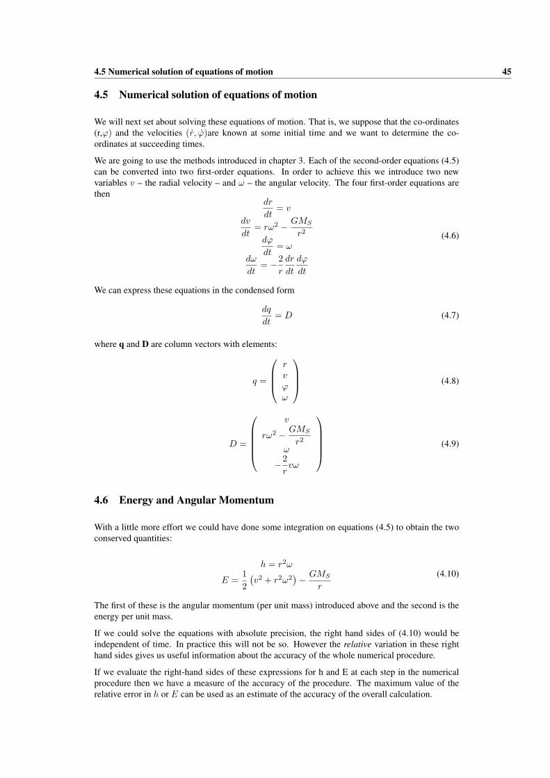
4.5 Numerical solution of equations of motion 45
4.5 Numerical solution of equations of motion
We will next set about solving these equations of motion. That is, we suppose that the co-ordinates(r,ϕ) and the velocities (r, ϕ)are known at some initial time and we want to determine the co-ordinates at succeeding times.
We are going to use the methods introduced in chapter 3. Each of the second-order equations (4.5)can be converted into two first-order equations. In order to achieve this we introduce two newvariables v – the radial velocity – and ω – the angular velocity. The four first-order equations arethen
dr
dt= v
dv
dt= rω2 − GMS
r2
dϕ
dt= ω
dω
dt= −2
r
dr
dt
dϕ
dt
(4.6)
We can express these equations in the condensed form
dq
dt= D (4.7)
where q and D are column vectors with elements:
q =
rvϕω
(4.8)
D =
v
rω2 − GMS
r2
ω
−2rvω
(4.9)
4.6 Energy and Angular Momentum
With a little more effort we could have done some integration on equations (4.5) to obtain the twoconserved quantities:
h = r2ω
E =12(v2 + r2ω2
)− GMS
r
(4.10)
The first of these is the angular momentum (per unit mass) introduced above and the second is theenergy per unit mass.
If we could solve the equations with absolute precision, the right hand sides of (4.10) would beindependent of time. In practice this will not be so. However the relative variation in these righthand sides gives us useful information about the accuracy of the whole numerical procedure.
If we evaluate the right-hand sides of these expressions for h and E at each step in the numericalprocedure then we have a measure of the accuracy of the procedure. The maximum value of therelative error in h or E can be used as an estimate of the accuracy of the overall calculation.
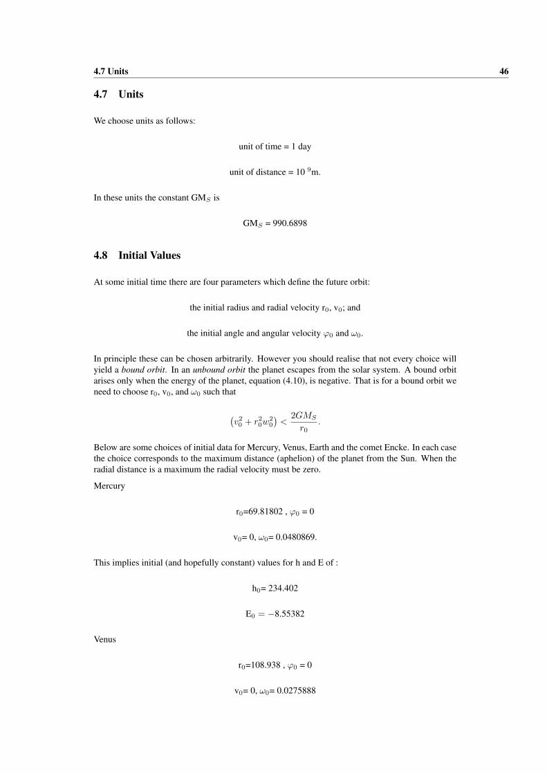
4.7 Units 46
4.7 Units
We choose units as follows:
unit of time = 1 day
unit of distance = 10 9m.
In these units the constant GMS is
GMS = 990.6898
4.8 Initial Values
At some initial time there are four parameters which define the future orbit:
the initial radius and radial velocity r0, v0; and
the initial angle and angular velocity ϕ0 and ω0.
In principle these can be chosen arbitrarily. However you should realise that not every choice willyield a bound orbit. In an unbound orbit the planet escapes from the solar system. A bound orbitarises only when the energy of the planet, equation (4.10), is negative. That is for a bound orbit weneed to choose r0, v0, and ω0 such that
(v20 + r2
0w20
)<
2GMS
r0.
Below are some choices of initial data for Mercury, Venus, Earth and the comet Encke. In each casethe choice corresponds to the maximum distance (aphelion) of the planet from the Sun. When theradial distance is a maximum the radial velocity must be zero.
Mercury
r0=69.81802 , ϕ0 = 0
v0= 0, ω0= 0.0480869.
This implies initial (and hopefully constant) values for h and E of :
h0= 234.402
E0 = −8.55382
Venus
r0=108.938 , ϕ0 = 0
v0= 0, ω0= 0.0275888

4.9 The Programme 47
The initial values for h and E are :
h0= 327.410
E0 = −4.57763
Earth
r0=152.0997 , ϕ0 = 0
v0= 0, ω0= 0.0166386.
The initial h and E are :
h0= 384.924
E0 = −3.31112
Comet Encke
r0=610.62 , ϕ0 = 0
v0= 0, ω0= 0.0001636.
The initial h and E are :
h0= 519.6
E0 = −0.5134
4.9 The Programme
An initial version of the programme is PLANETS.F95 and is on the Physics Intranet page. Youwill need to modify the programme so, after downloading the original, make a copy with a differentname such as PLANETS1.F95.
The planets program makes use of REAL KINDS. So before you get to grips with the program wewill investigate details of these. FORTRAN95 give the programmer some flexibility in the choiceof REAL variables. Suppose we decide we want to use real variables in the form
A× 10B
where A has at least 10 significant figures and the range of B includes −100 to +100. Then in theprogram we would declare an integer parameter
INTEGER, PARAMETER :: P=selected real kind(10, 100)
If the compiler can achieve what we want, P is returned as a positive integer that identifies theappropriate REAL KIND. Note that P itself is an integer that is used to label the particular real kind:it is NOT a real variable.

4.10 Kepler’s Laws 48
We can then use this integer parameter P to define REAL variables with the desired (or better)precision:
REAL (KIND=P) :: a, b, c
We can also use constants in the program to this precision as follows:
1.0 P, ,2.5 P
Notice that if we simply use 1.0 or 2.5 then these will only have the precision of the basic REALKIND (usually 6 digit accuracy).
If the compiler cannot achieve the desired accuracy then P is returned with a negative value and anyattempt to use it to define a REAL KIND will produce an error.
Now attempt Exercises 2 & 3 at the end of the chapter
4.10 Kepler’s Laws
Kepler (1571-1630) discovered his three laws of planetary motion by observation (of Brahe’s data)before Newton’s theory of gravitation. His first and second laws were published in 1609 and histhird in 1619.
First Law: Keplar’s first law states that the orbit of a planet is an ellipse with the Sun at onefocus.
How can we check whether our computed orbit is an ellipse ?
The equation of an ellipse, in the polar co-ordinates we are using, is
r =R
1− εcos (ϕ)(4.11)
where R and ε are constants defined by
R =h2
GMS(4.12)
ε =
√√√√(1 +2Eh2
(GMS)2
)(4.13)
ε is called the eccentricity. ε=0 corresponds to a circular orbit: the larger ε the more elongated theorbit. h and E are the angular momentum (per unit mass) and energy (per unit mass) defined earlier.
If we plot y=r versus x=R/(1 - εcos(ϕ)) then, if the orbit really is an ellipse, we should obtain astraight with slope 1 and abscissa 0.
Second Law: The radius vector sweeps through equal areas in equal times.
If in (small) time δt the angle ϕ changes to ϕ + δϕ then the area swept out by the radius vector isr2δϕ . Hence the area swept out per unit time is
r2 δ ϕ
δ t→ r2ϕ
Kepler’s second law implies that this is constant. However you should have already checked this(Exercise 3) under the guise of “conservation of angular momentum”.

4.11 Exercises 49
Third Law: The square of the period is proportional to the cube of the major axis.
Now attempt Exercise 4
4.11 Exercises
Exercise 1 [3 Marks]
How would the equation of motion of a particular planet change from (4.1) if we were to includeinteractions with other planets ?
The angular momentum of a particular planet will no longer be conserved if we include interactionswith other planets. Explain why and discuss the consequence for the orbit.
Exercise 2 [2 Marks]
Download the program kind test.f95 and explore the REAL KINDS that are available on the Salfordcompiler.
Exercise 3 [6 Marks]
Now download the planets.f95 program and compile and run the programme.
You will be prompted to choose a particular planet or comet; or to enter your own choice for theinitial values r0, ϕ0 ,v0 and ω0. Try the data given for Mercury, Venus, Earth and comet Encke andoutput the data to four separate files.
Record your observations. What is the period? What is the perihelion (minimum distance fromSun) and at what angle does it occur? Do this for a few time-steps and record your results.
Modify the program planets.f95 so that
h = r2ω
E = 12
(v2 + r2ω2
)− GMS
r
are evaluated initially and at each subsequent time-step. Output these values to a file.
Physics says that these two values should be constant. In fact because of the approximate calcula-tion they will fluctuate. The magnitude of the fluctuations is an indication of the accuracy of thenumerical procedure.
Use your results to estimate the accuracy of the numerical procedures for a few time steps for eachplanet.
Exercise 4: [6 Marks]
Check that the computed orbits are ellipses in the following way. In the program planets.f95 intro-duce allocatable arrays x, y and variables s, c, delta s, and delta c. Allocate the arrays x and ywith size n steps after the completion of the calculation of the orbit.
Then use a DO loop to read data into the variables x(j), y(j) from the disc file:
REWIND 15 ! This positions the file at its startDO j=1,n_steps
READ (15, FMT=’(5(2X,E14.6))’) t, q(1), q(2), q(3), q(4)! The above line should be essentially the same as the WRITE line! which stored the data! Notice that we have to read all the data in the record, even the! items we do not wanty(j) = q(1)

4.11 Exercises 50
x(j) = R/(one - epsi*cos(q(3)))END DOCALL Linfit(x, y, s, c, delta_s, delta_c)
The subroutine Linfit should be extracted from the file Stline.f95 and inserted into the ‘CONTAINS’section of the current programme.
The outputs s and c and their uncertainties delta s and delta c give a measure of the deviation ofthe orbit from an ellipse.
The above programme segment is only a guide. You should ensure that all the variables you use areproperly declared and that R and epsi should be given appropriate values.
Test the how well is the fit to an ellipse for a few time steps for each planet.
Using the data you have already obtained for Mercury, Venus, Earth & Encke, check the validity ofKepler’s third law. Note: the major axis is the sum of the minimum and maximum distances fromthe Sun. Again check the fit for several time steps.
Remember that you must finish your work on this chapter by writing an abstract in your logbooks.This abstract should summarize in less than 300 words what you have learnt and whether the ob-jectives of this chapter have been met.

Chapter 5
ANALYSIS OF WAVEFORMS
Version Date: Wednesday, 5 September, 2007 at 13:05
5.1 Objectives
In this chapter the main elements of Fourier Analysis are reviewed and the methods are applied tosome basic wave forms. On completion of this chapter students will have utilized simple numericaltechniques for performing Fourier Analysis; studied the convergence of Fourier series and how thisis effected by discontinuities in the function; and investigated the best choice of Fourier coefficientsin finite series. Fourier techniques will be applied to the solution of the diffusion equation.
5.2 Fourier Analysis
Fourier’s theorem states that any well-behaved (or physical) periodic wave form f(x) with periodL may be expressed as the series
f (x) =∞∑
r=−∞Fr exp (ikrx) (5.1)
where the wave-vector kr is given by
kr =2πr
L(5.2)
The complex Fourier coefficients Fr are given by
Fr =1L
∫f (x) exp (−ikrx) dx (5.3)
Here the integrals are over any complete period (e.g. x = 0 to x = L or x = −L2 to x = L
2 ).
The rth component of the sum in (5.1) corresponds to a harmonic wave with spatial frequency r/Land hence a wavelength L/r.
Normally, in Physics, f(x) is a real function. In this case the Fourier coefficients have the followingsymmetry property:
F∗r = F−r (5.4)
An important exception to this is the case of quantum mechanics where the wavefunctions arenormally complex. The above symmetry does not apply to this case.
51

5.3 The Numerical Methods 52
In numerical work we can only deal with series with a finite number of terms. Suppose the finiteseries, f [M ] (x), is used to approximate the function, f (x).
f [M ] (x) =M∑
r=−M
Fr exp (ikrx) (5.5)
The mean-square-error involved in making this approximation is by definition
E[M ] =1L
L∫0
[f(x)− f [M ](x)
]2dx. (5.6)
and this can be written (after quite a bit of manipulation!) as
E[M ] =+∞∑
r=−∞|F2
r| −M∑
r=−M
|F2r| (5.7)
This latter form shows that the mean square error decreases monotonically as a function of M (ieE[M+1]6 E[M ]). f [M ](x) converges to f(x) as more terms are added to the series. It can alsobe shown that the mean-square-error E[M ] (for any fixed M ) is minimized by using the Fouriercoefficients as calculated through equation (5.3).
5.2.1 Why bother?
It is not entirely clear from the above equations what has been gained by expressing the functionf(x) as a series (5.1) or (5.5).
In Physics we often need to evaluate the derivative (or second derivative etc) of a function: If thefunction has been expressed as a Fourier series then this is a trivial operation. For example the J thderivative of f(x), using (5.1), is
dJf (x)dxJ
=∞∑
r=−∞(ikr)
J [Fr exp (ikrx)] (5.8)
We can similarly write expressions for integrals of f(x).
5.2.2 Aperiodic functions
The instances, in Physics, of genuinely periodic functions are exceedingly rare. However there arestill many applications of the above theory.
Suppose a function f(x) either exists only in a finite range 0 ≤ x ≤ L or is known only in this finiterange. We can construct a periodic function simply by making a periodic repetition of the finite-range function with a repeat period L and apply the theory to this (artificial) periodic function. It isin this form that Fourier Analysis is normally applied in Physics.
5.3 The Numerical Methods
We now consider how to calculate the coefficients Fr.

5.3 The Numerical Methods 53
Figure 5.1. Trapezoidal Integration
In general we can approximate an integral by means of the trapezoidal rule. The essence of this isshown in the figure (5.1).
The integrand is divided into N equal intervals of size L/N and the integrand is approximated bya sequence of straight-line segments. The function f(x) is evaluated at the positions xs = sL/N .Note that N needs to be quite large to ensure accuracy. In the program you will use N has beentaken to be 1000.
The result of this procedure applied to (5.3) and is
Fr =1N
[(f(0) + f(L)
2
)+
N−1∑s=1
f
(sL
N
)exp
(−i
2π rs
N
)](5.9)
We can simplify this by defining an array
fs = f(
sLN
); s = 1, .., N − 1
f0 =(
f(0)+f(L)2
) (5.10)
Using this array gives the result for the coefficients as
Fr =1N
N−1∑s=0
fs exp(−i
2π rs
N
)(5.11)
This approximate procedure for the integrals predicts coefficients for |r| < N/2. It fails to correctlypredict coefficients for |r| ≥ N/2. That is it fails to predict the Fourier components with spatialfrequency greater than N/2L and wavelengths less than 2L/N.
In fact, if the function f(x) has no spatial frequency greater than N/2L, the Sampling Theoremtells us that the expression (5.11) is exact.
There is a technical problem in evaluating the exponentials in (5.11) or (5.5). In Fortran we canonly evaluate exp (iα) if α is not too large: In practice less than about 70. (You might think this is

5.4 Diffusion Equation 54
a deficiency of Fortran but you need to be aware that no other language has complex exponentialsbuilt in). We can surmount this difficulty by evaluating the exponentials in the form:
exp(−i
2π rs
N
)= exp
(−i
2π MOD (rs,N)N
)(5.12)
That is we have replaced rs by MOD (rs,N). This is a Fortran function which gives the remainderwhen rs is divided by N . This procedure works because (rs−MOD (rs,N)) /N is an integer andbecause
exp (−i2πm) = 1 (5.13)
for any integer m.
The argument of the exponential on the right-hand side of (5.12) is then a small quantity (in fact,less in magnitude than 2π).
If we only need to evaluate the original function f at the discrete points xs = sL/N then theformula (5.5) simplifies to
fs =M∑
r=−M
Fr exp(
i2π rs
N
)(5.14)
which is very similar to the expression for the Fourier coefficient (5.11) and the exponential iscalculated in the same way.
5.4 Diffusion Equation
I now look at the use of Fourier Analysis in solving differential equations.
In thermal equilibrium (and in the absence of external forces) gases and liquids have uniform den-sities. If a gas or liquid is prepared with a high density in a localized region then this excess densitywill quickly spread out until uniformity is restored: This process is called diffusion. If f(x, t)denotes the deviation of density from equilibrium then the evolution of this quantity with time isdetermined by the diffusion equation:
∂f (x, t)∂t
= D∂2f (x, t)
∂x2(5.15)
D is the diffusion constant.
Now suppose that I use equation (5.5) for f(x, t) but where the coefficients are functions of time:
f (x, t) =M∑
r=−M
Fr (t) exp (ikrx) (5.16)
Inserting this expression in the diffusion equation gives the following result for the coefficients:
Fr (t) = exp(−Dk2
r t)
Fr (0) (5.17)
This can be used to determine the density at any later time.

5.4 Diffusion Equation 55
If I assume this fluid is contained in a region
0 ≤ x ≤ L
then kr =2πr
Las in (5.2). The above equation then becomes
Fr (t) = exp
(−4π2 r2D t
L2
)Fr (0) (5.18)
The complete prescription for solving the diffusion problem is:
• Fourier analyse the initial (t = 0) density function. That is, calculate the Fourier coefficientsFr (0) using equation (5.11);
• Evaluate the coefficients at time t using equation (5.17);• Calculate the density at time t by inserting these Fourier coefficients into (5.5) with M =
(N − 1)/2.
Now attempt the exercises.
5.4.1 Exercises
1. [10 Marks](a) Obtain a copy of the program Fourier.f95 and run it. The program
sets up various waveforms and plots them in the graphics window.Make sure you understand how it works, and record its main featuresin your log-book. Remember that the graph-plotting routine alsowrites to the clipboard, so that copies of the graphs can be pastedinto other documents if required.
(b) Write a subroutine to calculate the coefficients Fr for |r| ≤ (N −1)/2 using equation (5.11). Write the results to a data file. Compareyour numerical results with the analytical solutions to equation (5.3)for one of the waveforms.
(c) Check that the symmetry property (5.4) is satisfied by the Fourier co-efficients. What symmetry do the square and triangular waveformshave, and how is this related to the values of their Fourier coeffi-cients? What about the ramp wave?
(d) Use your calculated values of Fr to reconstruct the approximationf [M ] in equation (5.14), and plot this curve alongside the originalwaveform. The value of M should be ≤ (N − 1)/2. Note that thesubroutine ‘plot graph’ provided will plot all the curves stored inf(npoints, ngraphs).
(e) Investigate the convergence of the series (that is gradually increaseM and observe what happens); does that of the triangular wave con-verge faster than those of the square or ramp waves? Also investigatethe Gibbs overshoot phenomenon observed in Fourier series for dis-continuous wave forms.

5.4 Diffusion Equation 56
(f) Calculate the mean-square-error in equation (5.7); Since N is large,
a good approximation to the right-hand side is(N−1)/2∑
r=−(N−1)/2
|F2r| −
M∑r=−M
|F2r|
(g) Show that E[M ] monotonically decreases with M .
Remember to keep an accurate record of your work in your log-book.
2. [7 Marks]Diffusion: Assume that in a diffusion problem the initial density isf (x, 0) = exp
(− (x−L/2)2
2σ2
)where σ = L
80 . Determine the densities
at times: t = L2
2000D , 2L2
2000D , 4L2
2000D . Notice that at t = 0 the requiredfunction is exactly that described as ”gaussian” in the program.
Remember that you must finish your work on this chapter by writing a summary in your laboratorynote books. This should summarize in about 300 words what you have learnt and whether theobjectives of this chapter have been met.
Chapter 6
EIGENVALUES AND EIGENVECTORS OFMATRICES
Version Date: Thursday, 30 August, 2007 at 10:20
6.1 Objectives
In this chapter you will investigate eigenvalue equations and eigenvalue packages for solving suchequations. You will be provided with a subroutine for finding all the eigenvalues and eigenvec-tors of a real symmetric matrix and also an eigenvalue package which finds a few eigenvalues andeigenvectors.
In the first set of exercises you will check that the results produced by the package against directcalculations (for small matrices).
In the second part of the project you will use the packages to investigate eigenvalues and eigenvec-tors of the Schrodinger equation.
6.2 Eigenvalues and eigenvectors of real symmetric or hermitian matrices
An eigenvalue equation is
A v(k) = λ(k) v(k) (6.1)
where A is an n× n matrix; v(k) is the kth eigenvector and is an n× 1 column vector; and λ(k) isthe kth eigenvalue.
The complete expression of the above equation is
n∑s=1
Arsv(k)s = λ(k) v(k)
r r = 1, . . . , n (6.2)
I shall only consider matrices that are real and symmetric or complex and hermitian:
In the first case the matrices have the symmetry
Ars = Asr
and in the second case
Ars = A∗sr
57

6.2 Eigenvalues and eigenvectors of real symmetric or hermitian matrices 58
These are the types of matrices required for most physical problems.
Such matrices have very special properties:
• all the eigenvalues are real;
• (if the matrices are n×n) there are n eigenvectors that are mutually orthogonal and these forma complete set.
Mutually orthogonal means that the eigenvectors satisfy
n∑r=1
(v(k)∗
r v(k′)r
)= 0 k 6= k′ (6.3)
It is conventional to normalize the eigenvector, that is choose them to satisfy
n∑r=1
(v(k)∗
r v(k)r
)= 1 (6.4)
The completeness of the eigenvectors means that any column vector can be constructed as a sum ofthe eigenvectors (with appropriate coefficients).
That is any column vector b can be written as
br =n∑
k=1
α(k) v(k)r (6.5)
The required set of coefficients α(k) can be evaluated by
α(k) =n∑
r=1
v(k)r
∗ br (6.6)
In order to emphasize that the properties of hermitian (or real symmetric) matrices are not shared bymore general matrices, consider a space of 2× 2 matrices and 2× 1 column vectors. A very simple,but not symmetric 2× 2 matrix is: (
0 10 0
)This matrix has eigenvalue λ = 0 and has only one eigenvector(
10
)
Clearly this one eigenvector cannot be used to generate an arbitrary 2× 1 column vector.
You should verify the above properties of this asymmetric real matrix.
The eigenvalue equation (6.1) can be written, entirely in matrix form, as
A V = V D (6.7)
where V is an n × n matrix which is made up from the n column vectors v(1),v(2), . . . ,v(n) andD is a diagonal matrix with diagonal entries λ(1), λ(2), . . . , λ(n).
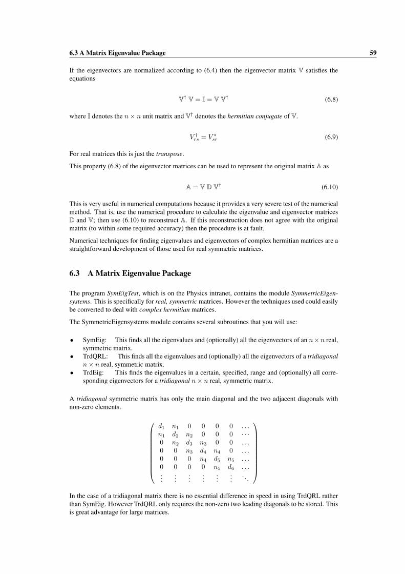
6.3 A Matrix Eigenvalue Package 59
If the eigenvectors are normalized according to (6.4) then the eigenvector matrix V satisfies theequations
V† V = I = V V† (6.8)
where I denotes the n× n unit matrix and V† denotes the hermitian conjugate of V.
V †rs = V ∗
sr (6.9)
For real matrices this is just the transpose.
This property (6.8) of the eigenvector matrices can be used to represent the original matrix A as
A = V D V† (6.10)
This is very useful in numerical computations because it provides a very severe test of the numericalmethod. That is, use the numerical procedure to calculate the eigenvalue and eigenvector matricesD and V; then use (6.10) to reconstruct A. If this reconstruction does not agree with the originalmatrix (to within some required accuracy) then the procedure is at fault.
Numerical techniques for finding eigenvalues and eigenvectors of complex hermitian matrices are astraightforward development of those used for real symmetric matrices.
6.3 A Matrix Eigenvalue Package
The program SymEigTest, which is on the Physics intranet, contains the module SymmetricEigen-systems. This is specifically for real, symmetric matrices. However the techniques used could easilybe converted to deal with complex hermitian matrices.
The SymmetricEigensystems module contains several subroutines that you will use:
• SymEig: This finds all the eigenvalues and (optionally) all the eigenvectors of an n×n real,symmetric matrix.
• TrdQRL: This finds all the eigenvalues and (optionally) all the eigenvectors of a tridiagonaln× n real, symmetric matrix.
• TrdEig: This finds the eigenvalues in a certain, specified, range and (optionally) all corre-sponding eigenvectors for a tridiagonal n× n real, symmetric matrix.
A tridiagonal symmetric matrix has only the main diagonal and the two adjacent diagonals withnon-zero elements.
d1 n1 0 0 0 0 . . .n1 d2 n2 0 0 0 · · ·0 n2 d3 n3 0 0 . . .0 0 n3 d4 n4 0 . . .0 0 0 n4 d5 n5 . . .0 0 0 0 n5 d6 . . ....
......
......
.... . .
In the case of a tridiagonal matrix there is no essential difference in speed in using TrdQRL ratherthan SymEig. However TrdQRL only requires the non-zero two leading diagonals to be stored. Thisis great advantage for large matrices.

6.4 Schrodinger Equation 60
For example if we are finding the eigenvalues of a 10000 × 10000 tridiagonal matrix then SymEigrequires 108 matrix elements to be stored (even if most of them are zero) whereas TrdQRL requiresonly 19999 elements to be stored.
Again, in the case of large matrices, both TrdQRL and SymEig provide too much information: Fora 10000× 10000 matrix there are 100, 000, 000 elements in the eigenvector matrix.
TrdEig allows the user to investigate a few eigenvectors.
These three subroutines are used as follows:
• CALL SymEig(A, eval, evec)A is the n × n matrix; eval is an n × 1 array containing the eigenvalues in ascending order;evec is the n× n eigenvector matrix.
• CALL TrdQRL(Ad, An, eval, evec)Ad is an n × 1 array containing the main diagonal elements of the matrix; An is an (n −1) × 1 array containing the leading upper diagonal elements of the matrix; evec is the n × neigenvector matrix, eval is an n× 1 array containing the eigenvalues.Ad(j) = A(j, j); An(j) = A(j, j + 1) = A(j + 1, j)Note: Some care is required in using this subroutine because on input evec needs to be setequal to the unit matrix.
• CALL TrdEig(Ad, An, Lower, Upper, NumEig, eval, evec)Ad is an n×1 array containing the main diagonal elements of the matrix; An is an (n−1)×1array containing the leading upper diagonal elements of the matrix; Lower and Upper definethe range in which the eigenvalues are required; NumEig is the number of eigenvalues (andeigenvectors) found in this range; eval is an n×1 array containing the eigenvalues in ascendingorder; evec is the n×NumEig eigenvector matrix.If there are more than certain number of eigenvalues in the range, the program will complain.The maximum number is set to 30 in the subroutine. If you really need more than this thenchange the variable max num eig.
One of the advantages of Fortran lies in the availability of good quality, well-tested ’libraries’ ofsubroutines. Most physicists make use of such subroutines and incorporate these in their programs.I produced the SymmetricEigenvalue module by modifying (to my own needs) subroutines from thewell-known library package LAPACK (Linear Algebra Package).
6.4 Schrodinger Equation
The time-independent Schrodinger Equation for a one-dimensional system is
− ~2
2m
d2Ψ(x)dx2
+ V (x) Ψ (x) = EΨ(x) (6.11)
This is an eigenvalue equation, with E as the eigenvalue and Ψ(x) as the eigenfunction. I want toshow how this differential eigenvalue equation can be expressed as a matrix eigenvalue equation.
The second derivative in (6.11) can be calculated (approximately) as
d2Ψ(x)dx2
=Ψ(x + ∆x) + Ψ (x−∆x)− 2Ψn (x)
∆x2 (6.12)
where ∆x is some suitably small distance.
I now define
Ψn = Ψ(n∆x) ; Vn = V (n∆x) (6.13)
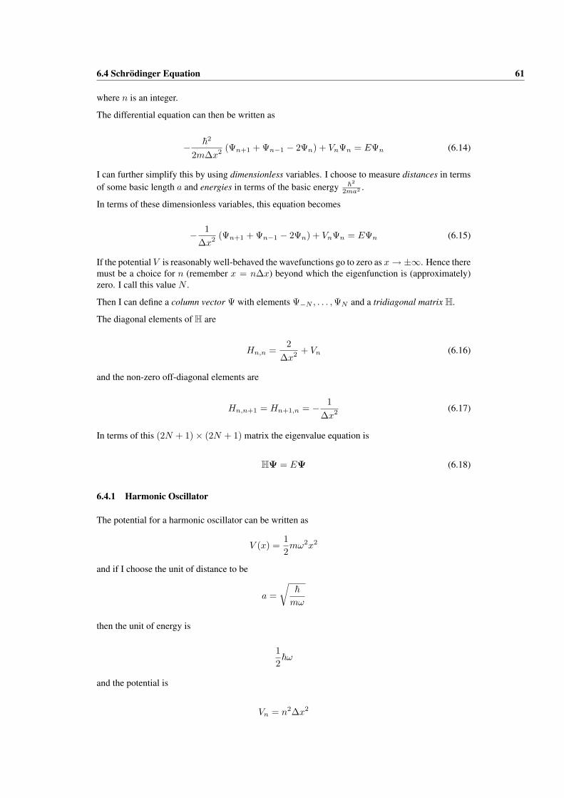
6.4 Schrodinger Equation 61
where n is an integer.
The differential equation can then be written as
− ~2
2m∆x2 (Ψn+1 + Ψn−1 − 2Ψn) + VnΨn = EΨn (6.14)
I can further simplify this by using dimensionless variables. I choose to measure distances in termsof some basic length a and energies in terms of the basic energy ~2
2ma2 .
In terms of these dimensionless variables, this equation becomes
− 1∆x2 (Ψn+1 + Ψn−1 − 2Ψn) + VnΨn = EΨn (6.15)
If the potential V is reasonably well-behaved the wavefunctions go to zero as x → ±∞. Hence theremust be a choice for n (remember x = n∆x) beyond which the eigenfunction is (approximately)zero. I call this value N .
Then I can define a column vector Ψ with elements Ψ−N , . . . ,ΨN and a tridiagonal matrix H.
The diagonal elements of H are
Hn,n =2
∆x2 + Vn (6.16)
and the non-zero off-diagonal elements are
Hn,n+1 = Hn+1,n = − 1∆x2 (6.17)
In terms of this (2N + 1)× (2N + 1) matrix the eigenvalue equation is
HΨ = EΨ (6.18)
6.4.1 Harmonic Oscillator
The potential for a harmonic oscillator can be written as
V (x) =12mω2x2
and if I choose the unit of distance to be
a =
√~
mω
then the unit of energy is
12
~ω
and the potential is
Vn = n2∆x2

6.4 Schrodinger Equation 62
This is a useful test problem because the exact results are known: The exact eigenvalues are:1, 3, 5, 7, . . ..
In order to solve numerically to a reasonable accuracy we need to choose
• ∆x 1• N∆x 1
In order to calculate the first few eigenvalues ∆x = 0.001 and N = 10000 should be sufficient togive fairly accurate results. However you may need to experiment with these values.
6.4.2 Spherically Symmetric 3D Systems
In a spherically symmetric 3D system the wavefunction in spherical polar coordinates can be writtenas
1rΨ(r) Ylm (θ, φ) exp (imφ) (6.19)
where Ylm are spherical harmonic functions. l and m are the angular momentum quantum numbers.
The radial function Ψ(r) satisfies the same equation as (6.11) except that a term
~2l(l + 1)2mr2
needs to be added to the potential; and, of course, r is positive.
For the case of the 3D harmonic oscillator, the eigenvalue equation can still be written as (6.18)except that the matrix indices now run from 1 → N and the potential is
Vn = n2∆x2 +l(l + 1)n2∆x2
In order to calculate the first few eigenvalues, for small values of l (l = 0, 1, 2), ∆x = 0.001 andN = 10000 should be sufficient.
In the case of the hydrogen atom, if we use the Bohr radius as the unit of distance, the correspondingpotential is
Vn = − 2n ∆x
+l(l + 1)n2∆x2
Exercises
1. [3 marks]
(a) Solve the eigenvalue equations for the 2× 2 asymmetric matrix(0 10 0
)Show the steps in process in detail. Show that it does not have a complete set of eigenvectors.
(b) Repeat the calculation for symmetric matrix(0 11 0
)

6.4 Schrodinger Equation 63
Discuss the differences.
(c) Determine the eigenvalue and eigenvector matrices D and V for the matrix in (b) and showthat equation (6.10) is satisfied.
2. [4 marks]
(a) Download the program SymEigTest.F95; make a working copy of this with a different name.
The program constructs a random n × n symmetric matrix, with n initially set to 10. It then callsSymEig to find all the eigenvalues and eigenvectors. (In fact it calls this 100 times just to make thecomputer time long enough to determine accurately!).
Then it uses equation (6.10) to attempt to reconstruct the original matrix. It finally calculates therms error in the reconstructed matrix (by comparing it to the original).
Run the program with matrix sizes 10, 20, . . . , 100. Record the results. Deduce how the time tooperate the subroutine depends on n.
(b) Modify the program so that the random symmetric matrix is now a random symmetric tridi-agonal matrix. Repeat the above calculations.
(c) Next modify the program to use the TrdQRL subroutine which is specifically intended fortridiagonal symmetric matrices. How does the performance compare with that of SymEig.
3. [4 marks]
Modify the program so as to make use of the subroutine TrdEig. Determine the lowest four eigen-values and corresponding eigenvalues of the 1D Harmonic oscillator and plot the correspondingeigenvectors.
4. [6 marks]
(a) Modify the program so as to be able to treat radial functions for spherically symmetric 3Dsystems. Test this by finding the first four eigenvalues for l = 0, l = 1 and for l = 2. Plot the lowestfour eigenfunctions for l = 2.
(b) Set up the eigenvalue equations for a the hydrogen atom; choose the Bohr radius to be theunit of distance. In this case suitable sizes of the parameters are: ∆x = 0.001 and N = 200000.Yes! you really are going to find eigenvalues of a 200000× 200000 matrix.
You may need to experiment with the parameters ∆x and N .
Find the first four eigenvalues for l = 0, l = 1 and for l = 2 and then plot the lowest foureigenfunctions for l = 2.
Note: In these dimensionless units the Coulomb potential is − 2(n∆x)
and the lowest eigenvalue
should be −1.
Remember that you must finish your work on this chapter by writing an abstract in your laboratorynotebooks. This abstract should summarise in about 300 words what you have learnt and whetherthe objectives of this chapter have been met.

Chapter 7
RANDOM PROCESSES
Version Date: Thursday, 30 August, 2007 at 11:21
7.1 Objectives
This chapter provides an introduction to random processes in physics. On completion, you will befamiliar with the random number generator in FORTRAN 95, and will have gained experience in us-ing it in two applications. You will also be ready to tackle later chapters that develop computationalstudies of random systems.
7.2 Introduction
It is convenient to describe models of physical processes as either deterministic or random. Anobvious example of the former is planetary motion and its description via Newton’s equations ofmotion: given the position and momenta of the particles in the system at time t, we can predictthe values of all the positions and momenta at a later time t′. Even the solution of Schrodinger’sequation is in a sense deterministic: we can predict the time evolution of the wave function in adeterministic way even though the wave function itself carries a much more restricted amount ofinformation than a classical picture provides.
The obvious example in physics of a theory based on randomness at the microscopic level is statis-tical mechanics. There may well be deterministic processes taking place, but they do not concernus because we can only observe the net effect of a vast number of such processes, and this is muchmore amenable to description on a statistical basis. But a statistical basis does not only concern sta-tistical mechanical (and thermodynamic) systems. Many physical systems are inherently disorderedand defy a simple deterministic analysis: the passage of a liquid through a porous membrane (oilthrough shale, for example), electrical breakdown in dielectrics, the intertwining of polymer chains,and galaxy formation are some examples of random processes.
Statistical mechanics uses concepts like entropy, partition functions, Boltzmann, Fermi or Bosestatistics and so on to describe the net effect of random processes. In computer simulations, oneactually models the microscopic random processes themselves. To model randomness, we needto have something to provide the element of chance - like a coin to toss, or a dice to throw. Ofcourse, in computing, we do not use coins or dice but rather random number generators to inject thestatistics of chance, and we start by seeing how they work.
64
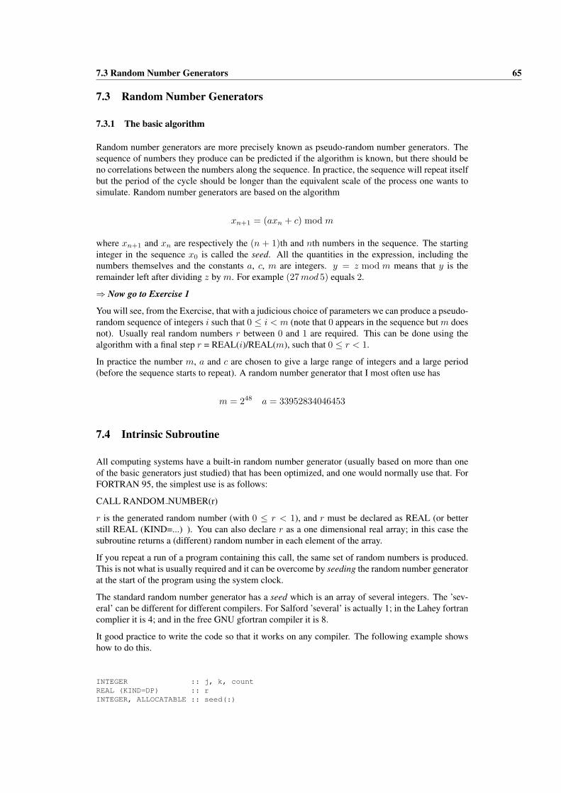
7.3 Random Number Generators 65
7.3 Random Number Generators
7.3.1 The basic algorithm
Random number generators are more precisely known as pseudo-random number generators. Thesequence of numbers they produce can be predicted if the algorithm is known, but there should beno correlations between the numbers along the sequence. In practice, the sequence will repeat itselfbut the period of the cycle should be longer than the equivalent scale of the process one wants tosimulate. Random number generators are based on the algorithm
xn+1 = (axn + c) mod m
where xn+1 and xn are respectively the (n + 1)th and nth numbers in the sequence. The startinginteger in the sequence x0 is called the seed. All the quantities in the expression, including thenumbers themselves and the constants a, c, m are integers. y = z mod m means that y is theremainder left after dividing z by m. For example (27 mod 5) equals 2.
⇒ Now go to Exercise 1
You will see, from the Exercise, that with a judicious choice of parameters we can produce a pseudo-random sequence of integers i such that 0 ≤ i < m (note that 0 appears in the sequence but m doesnot). Usually real random numbers r between 0 and 1 are required. This can be done using thealgorithm with a final step r = REAL(i)/REAL(m), such that 0 ≤ r < 1.
In practice the number m, a and c are chosen to give a large range of integers and a large period(before the sequence starts to repeat). A random number generator that I most often use has
m = 248 a = 33952834046453
7.4 Intrinsic Subroutine
All computing systems have a built-in random number generator (usually based on more than oneof the basic generators just studied) that has been optimized, and one would normally use that. ForFORTRAN 95, the simplest use is as follows:
CALL RANDOM NUMBER(r)
r is the generated random number (with 0 ≤ r < 1), and r must be declared as REAL (or betterstill REAL (KIND=...) ). You can also declare r as a one dimensional real array; in this case thesubroutine returns a (different) random number in each element of the array.
If you repeat a run of a program containing this call, the same set of random numbers is produced.This is not what is usually required and it can be overcome by seeding the random number generatorat the start of the program using the system clock.
The standard random number generator has a seed which is an array of several integers. The ’sev-eral’ can be different for different compilers. For Salford ’several’ is actually 1; in the Lahey fortrancomplier it is 4; and in the free GNU gfortran compiler it is 8.
It good practice to write the code so that it works on any compiler. The following example showshow to do this.
INTEGER :: j, k, countREAL (KIND=DP) :: rINTEGER, ALLOCATABLE :: seed(:)
7.4 Intrinsic Subroutine 66
CALL RANDOM_SEED(SIZE=k)ALLOCATE(seed(k))DO j = 1, k
CALL SYSTEM_CLOCK(count)seed(j) = count + j*j
END DO
CALL RANDOM_SEED(PUT = seed)
WRITE(*, *) ’Random number seed = ‘,seed
CALL RANDOM_NUMBER(r)
The first CALL of RANDOM SEED is to find out the size of the seed array and puts this sizeinto the integer k. The second call puts the correct seed array into the random number generator.Note, count (the current value of the system clock) is integer and that DP denotes what kind of realnumbers you are using.
It is sensible to write out the seed value just in case you do want to rerun the program with theexactly same set of random numbers.
7.4.1 Different number ranges
Often we want to generate random numbers over a range different from 0 to 1. This is straightfor-ward. If we want a real random number x between −2 and +2, for example, this can be obtainedfrom the random number generator output r using the statement: x = −2.0 + 4.0 ∗ r. Generally,use the expression x = a + (b− a) ∗ r if the required range is a to b.
We have to be a little more careful with integers. Suppose we were simulating the throw of a dice(and needed to generate a random integer from the set 1, 2, . . . .,6). If d is the required randominteger, we can use the statement: d = INT(6*r) + 1. Calculation of INT(6*r) gives one of theintegers 0, 1, . . . .,5.
7.4.2 Testing your random generator
The random generator is supposed to generate a random number r which is uniformly distributed inthe range 0 ≤ r < 1. If this is so then we can easily calculate the following average mathematically
〈rp〉 =1
p + 1
where p is any integer. We could then check the average computationally by generating N randomnumbers r1 . . . rN and then forming the average
〈rp〉 =1N
N∑k=1
rpk
When programming this it is not necessary to define an array for the random numbers!
For large N the two averages – theoretical and computational – should be very nearly the same andthe difference between them should reduce as N gets larger.
Note that for a large value of N it is not sensible to use the standard REAL variables since thesegive only about 1 part in 106 accuracy.

7.5 Monte Carlo Integration 67
A slightly more complicated test checks whether there is any correlation between neighbouringrandom numbers generated.
Suppose we have two independent random variables r and s then mathematically we have
〈rpsq〉 =1
(p + 1)1
(q + 1)
We then calculate this average using our computer random number generators. Generate N pairs ofrandom numbers (r1, s1) . . . (rN , sN ) and then form the average
〈rpsq〉 =1
N2
N∑j=1
N∑k=1
rpj sq
k
Again when programming this it is should not be necessary to define an array for the random num-bers!
There are more sophisticated tests but these simple tests should show if something is wrong withthe generator.
⇒ Now go to Exercise 2
7.5 Monte Carlo Integration
There is a wide range of calculations in Computational Physics that rely on the use of a randomnumber generator. Generally they are known as Monte Carlo techniques. We will start by lookingat the Monte Carlo method applied to integration. There are two approaches to choose from: the‘hit and miss’ method and the ‘sampling’ method.
7.5.1 Hit and Miss Method
Here is analogy to help explain the method. An experimental way to measure the area of the trebletwenty on a dart board is to throw the darts at the board at random; if N60 is the number hitting thetreble twenty and N is the total number of darts thrown, then the area A60 of the treble twenty isgiven by the equation A60 = A ∗N60/N , where A is the total area of the board.
⇒ Now go to Exercises 3(a) and (b)
7.5.2 Sampling Method
This method can be summarised by the equation
b∫a
f(x)dx =(b− a)
N
N∑i=1
f(xi)
Choose N random numbers xi in the range a < xi < b, calculate f(xi) for each, take the average,and then multiply by the integration range (b-a). It is similar to Simpson’s rule but in that case thevalues of xi are evenly distributed. We have seen already how to generate random numbers in therange a to b.
The extension to a multidimensional integral is easy. For example, in two dimensions, write
7.6 Nuclear Decay Chains 68
b∫a
dx
d∫c
dyf(x, y) =(b− a)(d− c)
N
N∑i=1
f(xi, yi)
In this case choose N pairs of random numbers (xi, yi) and go through a similar procedure. Theextension to an arbitrary number of dimensions is straightforward.
Generally, from the point of view of accuracy, it is better to use ‘conventional’ methods like Simp-son’s rule for integrals in low dimensions and Monte Carlo methods for high dimensions. If youhave body with an awkward shape, however, Monte Carlo methods are useful even at low dimen-sionality.
Why are Monte Carlo methods better in higher dimensions? If we pick n random numbers forour integration the error is proportional to n1/2 independent of the number of dimensions. For thetrapezoidal approximation and for Simpson’s rule the errors are proportional to n−1/d and n−2/d
respectively. Here n is the number of strips the integration range is divided into, and d is the dimen-sionality. Increasing n is more effective at reducing errors in Monte Carlo than in the trapezoidalrule for d > 2. In comparison with Simpson’s rule, Monte Carlo wins out for d > 4.
⇒ Now go to Exercises 3( c) and (d)
7.6 Nuclear Decay Chains
Now let us consider a nuclear decay sequence with a number of different daughter products:
23492 U −→
250,000yr
23090 Th + α
↓ −→80,000yr
22688 Ra + α
↓ −→1,620yr
22286 Rn + α
↓−→fast
20682 Pb
The times shown are half-lives in years. 23492 U is produced from 238
92 U by a decay with a half-life of4.5×109 years which is so long compared with the half lives in the above chain that we can ignorethis factor in the change of the number of 234
92 U nuclei. The decay of 22286 Rn to 206
82 Pb (stable) is bya chain of disintegrations and takes place very rapidly on the time-scale being considered here; T1/2
for 22286 Rn is about 4 days. Therefore we can in effect consider the decay of Ra to be directly to the
stable Pb isotope.
The half life of a nucleus is defined as the time taken for a half of the nuclei in a large populationto decay. For an individual nucleus it really is a random process however with only the probabilityof decay defined. We can either use an analytic method or a computer simulation to describe thesystem.
7.6.1 Analytic approach
In the analytic approach we deal with the statistical averages of the numbers of each type of particle.These average quantities are not, of course, integers.
Let N1(t) be the statistical average of the number of 23492 U nuclei at time t,
N2(t) be the statistical average of the number of 23090 Th nuclei at time t,
N3(t) be the statistical average of the number of 22688 Ra nuclei at time t,
and N4(t) be the statistical average of the number of 20682 Pb nuclei at time t.

7.6 Nuclear Decay Chains 69
Note that because we are considering the statistical averages these numbers are no longer integers.
We take the initial condition (at t = 0) to be N1 = N; N2 = N3 = N4 = 0.
At a general time t, N1(t) + N2(t) + N3(t) + N4(t) = N, i.e. the total number of nuclei is conserved.
The rate equations for the chain of decays are:
dN1
dt= −λ1 N1
dN2
dt= λ1 N1 − λ2 N2
dN3
dt= λ2 N2 − λ3 N3
dN4
dt= λ3 N3
where the decay constant λ = ln2/T1/2= 0.693/T1/2
.
The analytic solution to these equations with the given initial conditions is
N1(t) = N exp(−λ1 t)
N2(t) =λ1 N
λ2 − λ1[exp (−λ1 t)− exp (−λ2 t)]
N3 (t) = λ1 λ2 N
exp(−λ1 t)
(λ1 − λ2) (λ1 − λ3)+
exp(−λ2 t)(λ2 − λ3) (λ2 − λ1)
+exp(−λ3 t)
(λ3 − λ1) (λ3 − λ2)
N4 (t) = N − N1(t) + N2(t) + N3(t)
7.6.2 Computer simulation
We are now going to take a different approach in which we try to simulate the random physicalprocesses. We can regard a nucleus as existing in one of 4 states as defined as above:
State 1 ≡ U ; state 2 ≡ Th ; state 3 ≡ Ra ; state 4 ≡ Pb
The probability PI that a nucleus in state i decays within a time interval ∆t to the next state (i+1) isgiven by Pi = λi∆t. When it reaches state 4 there is no further decay, of course. We suppose that∆t is small enough for the possibility of double decays such as
U → Th → Ra
within ∆t to be negligible.
We can simulate the decay process for one nucleus by choosing a random number in the range 0 to1 and comparing this with Pi. If the random number is less than Pi then the decay takes place; if notthe nucleus remains in the same state. This trick is very common in computer simulations of randomprocesses.
We start with N nuclei in state 1, and simulate the decay of each one of the nuclei in a successionof time intervals ∆t.
In such a computer simulation the numbers of each type of particle are of course integers as theyare in the real physical case.
⇒ Now go to Exercise 4

7.7 Exercises 70
7.7 Exercises
1. [2 Marks]
Check on paper that you understand what is happening. Take a=5, c=2, m=8, and x0 =1 and generatethe first few random numbers. You should find they start as follows 1, 7, 5, 3, and then repeat. Nowgo through the same process with the following sets of numbers: (a=3, c=4, m=8, x0 =1) and then(a=5, c=1, m=8, x0 =1). Record your sequences of numbers.
2. [ 4 Marks]
(a) Write a program which tests the built-in random number generator by calculating the averages〈rp〉 for a few values of p, in the range 1 to 12. Do this for the cases where the number of randomnumbers generated N is 100,000, 1,000,000 and 10,000,000. Record your test results.
(b) Modify the program to calculate the averages, using the built-in random number generator,〈rpsq〉 for a value of p, q in the range 1 to 12. Use a double summation to do this;
〈rpsq〉 =1
N2
N∑j=1
N∑k=1
rpj sp
k
where N is 1000 and 10,000. Record your test results.
3. [ 5 Marks]
(a). We will use the random number generator to calculate π. Consider a circle of radius 1 unit andcentre at the origin (0,0); it just fits in a square with corners at the points (-1,-1), (-1,+1), (+1,-1),(+1,+1). Now generate a pair of random numbers (x,y) each between -1 and +1. They are insidethe square. What is the condition for them to be inside the circle as well? Repeat this till you havegenerated a total of N points. If Nc points were also inside the circle, the ratio of the area of thecircle to that of the square is Nc/N - but the area of the square is 4, so the area of the circle is givenby 4Nc/N. But since we know the answer is πr2 and r=1, we have a way of determining π. Write aprogram to do this. You should aim for this kind of accuracy: π=3.14±0.01.
(b). Although we expressed it as an evaluation of π, the last exercise was really a calculation of thearea of a circle. We know that the area of a circle of radius r is given by A=πr2. The analogousquantity in 3 dimensions is the volume of a sphere, V=(4/3)πr3. What is the equivalent quantity in4 dimensions? Presumably the ‘hypervolume’ of a 4D ‘hypersphere’ of radius r is given by H=Cr4.Make (very minor) modifications to your circle program to calculate C. [exact result is C=π2/2].
(c). The mean energy (kinetic) of an atom of a Boltzmann gas of non-interacting atoms moving in1 dimension is given by
E = I1/I2where
I1 =∞∫−∞
(p2/2m) exp(−p2/2mkT
)dpand I2 =
∞∫−∞
exp(−p2/2mkT
)dp
p is the momentum. With a change of variables, α=p/√
(2mkT), this can be rewritten as
E = kT (J1/J2)where
J1 =∞∫0
α2 exp(−α2
)dαand J2 =
∞∫0
exp(−α2
)dα
Write a program that employs the sampling method to calculate J1 and J2 and thus the coefficientJ1/J2. You will have to cut off the upper limit of the integrals at some value b. Increase the values ofb and N until you have a result that is accurate to 2 decimal places, but estimate a reasonable valueof b by hand before you start computing (for what value of α does the integrand become small). Isyour result what you expect?

7.7 Exercises 71
(d). Now calculate the mean energy (translational kinetic energy + vibrational potential energy) ofan ideal gas of diatomic molecules confined to 1 dimension. It is a 3 variable problem - the momentap1 and p2 of the 2 atoms of the molecule and their displacement x from the equilibrium separation.Besides kinetic energy terms p2
1/2m and p22/2m we have a potential term µω2x2/2 where µ is the
reduced mass and ω is the natural frequency. If we again do a change of variables, β=x√
(µω2/2kT),we can write an expression for E as in the previous case, but now
J1 =
∞∫0
dα1
∞∫0
dα2
∞∫0
dβ(α2
1 + α22 + β2
)exp
[−(α2
1 + α22 + β2
)]
J2 =
∞∫0
dα1
∞∫0
dα2
∞∫0
dβ exp[−(α2
1 + α22 + β2
)]What is the coefficient of kT in this case? What result did you expect to obtain?
4 [ 6 Marks]
Compile and execute the program Nuclear Decay.f95. This does the analytic part of the calculationand prints out the results every 50,000 years up to 2,000,000 years. It asks you to input the numberof nuclei N, and a time step dt. Use 1.0 for dt for the moment (dt is not relevant until you write theMonte Carlo code). Parts of the program relevant for only the Monte Carlo part are indicated bycomments. When you have understood the program you can go onto the Monte Carlo part.
An array nr(1 : 4) has been set up for you which holds the number of nuclei of each type. nr(2 : 4)have been initialized to zero and nr(1) to the total number of nuclei. That is, initially each nucleusis of type 1.
Your task is to write a subroutine for the MC calculation and incorporate it in the program. Theprogram is set up so that your subroutine can be called each time step to calculate the updatedvalues of nr. In each time step you have to consider each nucleus and determine whether it decaysusing the criterion given in the text. Notice that the sum
4∑j=1
nr(j)
should remain constant.
First choose a reasonable time step and justify your choice. Now run your program with variousnumber of atoms in your sample, say 100, 1000, 10000 and 100000. What sort of value of N(number in the program) do you need to use for analytic and MC results to be similar. Display andcomment on results that you obtain.

Chapter 8
MONTE CARLO SIMULATION
Version Date: Wednesday, 1 October 2003
8.1 OBJECTIVES
The Metropolis Monte Carlo algorithm is one of the most important techniques in ComputationalPhysics for dealing with random systems; it also provides a way of including temperature into themodelling. The main objective of this chapter is to introduce Monte Carlo methods. Inevitablymodelling is done on systems with a small number of particles, whereas in real systems we aredealing with ∼1023 particles. Fluctuations about the mean become a dominant feature in smallsystems and it is important that we understand about size effects. Developing a feeling about thissubject is the first priority of this chapter. A simple model contains the main features.
8.2 EQUILIBRIUM AND FLUCTUATIONS
Suppose we have two boxes, one of which contains a certain number of molecules of a gas andin the other is a vacuum. If these boxes are joined then gas will flow from one to the other untilequilibrium is reached (a state of uniform density).
To define fully a state of the system we have to specify the position and momentum of each moleculeof the gas. Let us investigate the approach to equilibrium with a drastic simplification. We willconcern ourselves only with which box a molecule is in, and ignore details about positions andvelocities.
Suppose there are N molecules in total and, at each instant, NL are in the left hand box and NR arein the right hand one (of course, NL + NR = N). The table below describes the possible situationsfor N=6. There are N+1 states of the system distinguished by the number of molecules in each box.
State NL NR No. of configura-tions, Ω
Prob.L to R
Prob.R to L
lnΩ
1 6 0 1 1 0 0.0002 5 1 6 5/6 1/6 1.7923 4 2 15 2/3 1/3 2.7084 3 3 20 1/2 1/2 2.9965 2 4 15 1/3 2/3 2.7086 1 5 6 1/6 5/6 1.7927 0 6 1 0 1 0.000
The number of configurations (or microstates) associated with a particular state is given by Ω =N !/(NL!NR!). In the above example, Ω of state 2 is 6 because any of the 6 molecules could be theone in the right hand box (molecules here are treated as classical – they are distinguishable). The
72

8.3 MONTE CARLO SIMULATIONS – THE PRINCIPLES 73
entropy S of a particular state is given by S/kB=lnΩ.
As the system evolves, suppose one molecule moves from one box to the other in each time step. Itis reasonable to take the probability that it will be a left to right move as NL/N and for a right toleft move as NR/N . It is clear from the table that the tendency will be a move toward state 4 (theequilibrium state - the one of maximum entropy), but there will certainly be fluctuations about thisposition.
Even if we are in the equilibrium state, there is a chance that fluctuations could lead us in a few timesteps into a state where all the molecules are back in one of the boxes. The probability (see table)that this occurs in just three time steps is (1/2)x(1/3)x(1/6)=1/36. This is not extremely long odds,but think what is the likelihood of a similar situation occurring for larger values of N.
The program boxes.f95 simulates the above model. You can enter N and the number of time-steps;you can select to start with the particles equally distributed or all in the left hand box; you can alsochoose graphical output. The random number generator decides on a L to R or R to L move. Lookat the program and make sure you understand what it does.
⇒ Go to Exercise 1(a)
Now let us try to get something more quantitative about the fluctuations from the simulations. Thevariance σ2 is defined as:
σ2 =< N2L > − < NL >2
and σ provides us with a measure of the size of the fluctuations. The averages (denoted by angularbrackets) are taken over the time period of the simulation. The ratio σ/ < NL > is an informativeway to express the behaviour.
⇒ Go to Exercise 1(b)
You will have observed in Exercise 1(a) that if N is small, then quite frequently you find all of theparticles in one of the boxes; by contrast, if N is large, this dramatic departure from equilibriumis an extremely rare event. We can make this observation more quantitative. Let us assume thatthe probability that there are NL particles in the left-hand box is given by a normal (Gaussian)distribution with width σ:
P (NL) =(σ√
2π)−1
exp[− (NL− < NL >)2 /
(2σ2)]
Given the values of < NL > and σ (see Appendix), we could argue that the probability of findingall or none of the particles in one of the boxes is
2√
2/πN exp (−N/2)
Then, the number of times in a run that we will find all the particles in one box is the product ofthis probability and the number of time-steps. Note, this argument is only a rough one, but it shouldgive an order of magnitude estimate.
⇒ Go to Exercise 1( c)
8.3 MONTE CARLO SIMULATIONS – THE PRINCIPLES
We have to find a way to introduce temperature into a simulation. In statistical mechanics we cancalculate a thermodynamic average of some quantity A by performing a weighted sum over allconfigurations (microstates) of the system

8.4 The Metropolis Monte Carlo Algorithm 74
< A >= Z−1∑
s
As exp(−Es/kBT )
where As is the value taken by A in microstate s, and Z is the partition function
Z =∑
s
exp(−Es/kBT )
In a computer simulation, what we would like to do is perform a trajectory through phase spacein such a way that a microstate s is visited with a probability exp(−Es/kBT )/Z. Averaging Athroughout the trajectory will then reproduce the same < A > that we get in the statistical mechanicscalculation (canonical ensemble).
There is not a unique way of doing this but one of those most widely used is the Metropolis MonteCarlo algorithm.
8.4 The Metropolis Monte Carlo Algorithm
The algorithm is best described by way of an example. Suppose we have a system of N spins(elementary magnets) each of which can point up or down. There are 2N microstates of the system;a microstate is determined by specifying each spin (up or down) of the system. We assume thatthe spins interact with each other in some way so that the energy associated with any microstate isknown. A trajectory through phase space governed by the algorithm is generated as follows.
(i) Choose one of the 2N microstates in which to start.(ii) Pick one of the spins at random (using the random number generator).(iii) Consider the new microstate obtained by reversing the direction of the selected spin; calculate
the change in energy ∆E that occurs if the system is allowed to jump to the new microstate.(iv) If there is a decrease in energy, ∆E ≤ 0, move to the new microstate state (ie flip the selected
spin);(v) If there is an increase in energy, ∆E > 0, make the move with a probability exp(−∆E/kBT );
ie on some occasions, when ∆E > 0, the jump is made, while on others the system remainsunchanged.
(vi) Repeat the process from (ii) until enough data is collected.
The example used for illustration is a simple discrete one in which each entity (a spin) has onlytwo possible states. We could equally well apply the principle to an assemblage of particles (in afluid say). In that case step (ii) would be to pick a particle at random, and step (iii) would involvecalculating the change in potential energy if its position was changed randomly by a small amount.
Note that step (iv) is what defines the Metropolis algorithm. One could use alternative recipes thatwould still provide a valid simulation of the canonical ensemble (see Mathematical Appendix 2 forthe condition that has to be fulfilled). The Metropolis method is the most widely used however, andwe will not consider other choices.
8.5 The Ising Model
The spin system used in the introduction to the Metropolis algorithm is known as the Ising model.The energy of a pair of spins is generally written as −J if they are parallel and +J if they areantiparallel. A positive J provides a simple model for ferromagnetism and a negative one for anti-ferromagnetism. The table summarises the situation for a single pair of spins for which there are 22
microstates.
8.6 The Ising Model and the Monte Carlo Algorithm 75
If we represent a spin numerically as S = +1 (up) and S = −1 (down), then the energy of the pair,S1 and S2, can be written: E = −JS1S2.
Microstate Spins Energy1 ↑↑ −J2 ↑↓ +J3 ↓↑ +J4 ↓↓ −J
Although the Ising model was originally set up to study the transition from ferromagnetism toparamagnetism as temperature is increased, it has much wider application. We could, for example,use it to describe a binary alloy (made up of atomic species A and B). We use spin up to representtype A and spin down to represent type B. Then if J > 0, atoms like to have their own sort asneighbours and, if J < 0, they prefer the other type as neighbours.
8.6 The Ising Model and the Monte Carlo Algorithm
Let us fill in a little more detail about the implementation of the algorithm (see the working programising.f95). Suppose the spins lie on a lattice (square in 2 dimensions, cubic in 3 dimensions). Eachspin has 4 (in 2D) or 6 (in 3D) neighbours (the program is for 2D).
Declare an array, spin(:, :), the elements of which can take values ±1. The arguments of the arraylabel its position coordinates. Then initialise the array (step 1 of the MC algorithm). The 3 commonchoices are programmed.
−∑j
JijSiSj Now choose a spin at random (step 2). Let us call it spin i defined by its coordinates
(x,y). The energy associated with it and its neighbours is
∆E = 2∑j
JijSiSj where j is summed over the neighbours. The change in energy (step 3) on
reversing the sign of Si is therefore 4∑j
JijSj . If the spin flip is made in step 4, Si → −Si. In
the calculations, only the dimensionless ratio, J/kBT is important. Usually in programming J is setequal to 1 and ‘temperature’ is a number that we can vary. If we wanted to convert the ‘temperature’in the program to real units we would multiply it by J/kB .
Periodic boundary conditions are usually employed to reduce finite size effects - otherwise the spinson the edges of the lattice would have fewer than 4 (in 2D) neighbours. This is done by adding anextra row of spins to each edge – each spin is constrained to have the same value as the one justinside the lattice on the opposite side.
8.7 Rationale
The reason for doing simulations, of course, is that we are trying to work out the behaviour ofmacroscopic systems containing of the order of 1023 spins or particles, and there are only a fewmodels for which exact statistical mechanical solutions are obtainable. Hopefully we can simulateon systems with N large enough so that we can deduce (or extrapolate to) what happens in themacroscopic case (even though N is many orders of magnitude smaller than 1023).
You might well ask, if we have to be satisfied with a reasonably modest value of N , why not do anexact calculation for that size of system. Considering a spin system will provide the answer. For anexact calculation one would have to consider 2N states and perform thermodynamic averages overthem. For a Monte Carlo simulation you would consider perhaps 1000 ×N Monte Carlo steps. If1000×N ¡ 2N it is more cost effective to do a Monte Carlo calculation. Check at what value of N

8.8 MONTE CARLO SIMULATIONS – IN ACTION 76
the cross-over occurs and MC becomes more efficient (you will find it is between 13 and 14 - reallyvery small). Even for a fairly modest N , the value of 2N rapidly becomes too large for an exactcalculation.
A Monte Carlo simulation is employing the principle of importance sampling. At low temperatures,the low energy states dominate in a thermodynamic average - and the phase space excursion isprimarily through these microstates. Indeed in a real macroscopic system the high energy stateswill rarely get visited at low temperatures - perhaps on a time scale of the order of the age of theUniverse - or longer! At very high temperatures, on the contrary, all microstates are more or lessequally accessible - but a fairly coarse-grained average will do - as long as representative microstatesare visited according to their relative density.
The fact that simulations are done on finite systems has to be borne in mind. There are ways ofextrapolating to large systems from a series of simulations on small systems over a range of differentsizes. Even if we do not want to go to such extra sophistication, we generally do have a knowledgeof what the effects of finite size are; we have seen one example of this already in the calculation ofσ/ < NL > in the previous section.
8.8 MONTE CARLO SIMULATIONS – IN ACTION
Because MC simulations are such an important technique, we have looked at the principles in somedetail. Now let us put it into practice.
⇒ Go to Exercise 2(a)
8.9 Order Parameter - Magnetisation
The magnetisation per spin S at a particular instant in time is defined as
S = N−1∑
r
Sr
where the sum is over all N spins of the lattice. The average over the period of the simulation,< S >, is our definition of the magnetisation. We expect it to be 1 at very low temperaturesand to fall as temperature is increased going to zero when T reaches TC (the model exhibits a Curietemperature). For this reason it is a convenient measure of the order in the system – and is sometimescalled the order parameter. It is also possible to study the fluctuations in the magnetisation: < S2 >− < S >2. The fluctuations are largest at temperatures near TC . They are also related to thesusceptibility (the ease with which the system responds to a magnetic field) – see Appendix.
⇒ Go to Exercise 2(b)
8.10 Temperature Scan (Annealing and Quenching)
If you want to look at several temperatures in a simulation, it is usually more efficient to do themall in a single run. The spin configuration at the end of the simulation at one temperature providesthe input for the simulation at the next temperature. The procedure increases efficiency because itreduces the time to settle to equilibrium compared with making a new start at each temperature.
There is another problem, which you might have noticed, and this can be avoided by this technique.At low temperatures, you might have expected that your picture would have been all red or all blue(fully ordered). For larger samples at T = 0.5, say, it is more likely that you will see a big blue anda big red area. Early on, one part of the sample started ordering one way while the other began with
8.11 MATHEMATICAL APPENDIX 77
the opposite orientation. Neither could win. This is what happens in reality. If you cool somethingvery fast – ‘quenching’ – it does not have time to adjust and different parts get locked into positionsthat are not necessarily the most favourable energetically for the system as a whole. A slow coolingschedule (annealing) will give them time to adjust.
⇒ Go to Exercise 2(c)
8.11 MATHEMATICAL APPENDIX
8.11.1 Fluctuations
If ΩNNL
is the number of configurations of the state with NL molecules in the left-hand box when Nmolecules are present then
< NL >= Z−1N∑
NL=0
NLΩNNL
< N2L >= Z−1
N∑NL=0
N2LΩN
NLZ =
N∑NL=0
ΩNNL
where
ΩNNL
= N !/ [NL!(N −NL)!]
Now ΩNr is also the coefficient that appears in the binomial expansion of (1 + x)N SN = (1 +
x)N =N∑
r=0ΩN
r xr
Setting x=1, we obtain
Z = 2N (there are 2 configurations of each particle and there are N of them)
Then, differentiating:
dSN
dx= N(1 + x)N−1 =
N∑r=0
ΩNr rxr−1
and again setting x=1 and comparing the expression for < NL >
< NL >= Z−1N2N−1 = N/2
A further related differentiation yields
d
dx
(xdSN
dx
)= N(1 + x)N−1 + N(N − 1)x(1 + x)N−2 =
N∑r=0
ΩNr r2xr−1
and following an analogous procedure for < N2L > we obtain
< N2L >= Z−1
[N2N−1 + N(N − 1)2N−2
]= N/2 + N(N − 1)/4
From the definition of the variance σ2 =< N2L > − < NL >2 we obtain
σ2 = N/4 and σ =√
N/2
and so finally

8.11 MATHEMATICAL APPENDIX 78
σ
< NL >=
1√N
8.11.2 Metropolis Monte Carlo Algorithm and Principle of Detailed Balance
An important relation that has to be satisfied in simulations of the sort we are considering is calledthe Principle of Detailed Balance; it can be written as
P (i → j) exp(−Ei/kBT ) = P (j → i) exp(−Ej/kBT )
where P (i → j) is the probability that the system, if it is in microstate i, will make a transition tomicrostate j; Ei is the energy of the system when in microstate i.
Since the probability of the system being in microstate i is given by Z−1exp(−Ei/kBT ), we cansee that the left hand side of the equation gives the rate at which transitions from i to j occur, andthe right hand side describes the reverse process. The detailed balance equation is the condition forequilibrium.
For a computer simulation, the condition on any P (i → j) that is used is that it must satisfy thedetailed balance equation. We can see that the Metropolis algorithm does. Suppose that Ei > Ej .Then according to the algorithm, P (i → j) = 1, and P (j → i) = exp[−(Ei − Ej)/kBT ], whichis entirely consistent with the detailed balance requirement.
8.11.3 Susceptibility and Fluctuations
We can write the mean value of the spin at an arbitrary site i as
< Si >= Z−1∑
Si exp [−β (E − SiH)]
where
Z =∑
exp [−β (E − SiH)]
and β = 1/kBT . The sum is over all configurations (with energy E) of the system; we includea magnetic field H and show the contribution to the energy arising from the effect of H on theparticular spin.
The susceptibility χ is defined as
χ =d < S >
dH
d [Z < Si >]dH
=< Si >∑
βSi exp [−β (E − SiH)]+Zd < Si >
dH=∑
βS2i exp [−β (E − SiH)]
Now dividing both sides by Z leads us to
d < Si >
dH= β
[< Si >2 − < S2
i >]
< Si > is the same for all sites, so we can write

8.12 EXERCISES 79
χ =[< S2 > − < S >2
]/kBT
8.12 EXERCISES
1 [8 Marks]
(a). Run the program with the graphics option to get a feel for what happens. Compare N=10,tstep=200 with N=100, tstep=5000 for example. Choose other values as well. Describe your obser-vations.
(b). Add some code to the program to calculate < NL >, < N2L >, σ, and the ratio σ/ < NL >.
You will need to calculate values averaged over the run; do several runs for a particular set ofparameters (the clock will ensure different random number sequences); start with the configurationof equally filled boxes. If you are doing the averages for very large samples or over long timeperiods, be careful about generating very large numbers. If you are working with integers try toestimate how big an integer your program is likely to produce. The default ‘KIND’ for integers onFORTRAN 95 is 3 which means integers in the range −231 to 231 − 1 are allowed. If you find youare going above this range, convert to floating point for calculating averages. Compare the resultsfrom your simulations with the ‘theoretical’ values from the Mathematical Appendix. In particular,investigate how σ/ < NL > depends on N. You can speed up the calculation by not displaying thegraphical output.
(c). Add some more lines to the code to count the number of times in a run that all or none of theparticles is in the left-hand box. Sometimes this configuration never occurs, so write some code toevaluate the largest and smallest value of NL that occurs in a run. Compare your simulation withthe rough theory. You should be able to do the investigations for N up to around 20. Use the roughformula to estimate the probability of the rare event occurring for N = 50, and calculate how longyou would have to sit in front of the computer to observe it.
2. [ 9 Marks]
(a). The program ising.f95 allows you to input lattice size, number of Monte Carlo steps per spin,temperature, and sign of the coupling J. You can choose from three initial configurations and youcan select graphical output (up and down spins are distinguished by red and blue circles). You canalso request a metafile for hardcopy output. The colour output is relatively slow: use it to get a feelabout what is happening, but switch it off for quantitative calculations.
First study the program and make sure that you understand what it does. Do a number of runs fordifferent parameters and comment qualitatively on what happens. Examine values of temperature0.5, 2.0, 3.0, and lattices of side 16 and 64. Monte Carlo steps per spin in the range 200-500 shouldbe adequate at this stage. It may help your comments to note that the model is expected to show aCurie temperature TC = 2.27J/kB (2.27 in the program units).
You can also try the other options.
(b). As a first step to more quantitative results, add some code to the program to monitor themagnetisation. Calculate the total spin Stot =
∑r
Sr immediately after initialisation. Then each
time the Metropolis step produces a spin flip, update Stot by +2 or −2.
Now average the magnetisation over the simulation run, and also find how the magnetisation fluc-tuates. That is, calculate both < S > and < S2 > − < S >2.
If the simulation starts far from equilibrium, you should let the system settle down until it is fluctu-ating about its equilibrium behaviour before you start your averaging. For example, you might use1000 MC steps per spin, but let it run for 200 steps per spin before you start averaging (ie disregardthe first 20% of the run).

8.12 EXERCISES 80
The total number of MC steps (see program) is mcs=mcsps*n. It is not necessary to average thespin over all of the mcs steps. You could save time by including in your average values taken everyn MC steps, for example.
Referring to ising.f95, the suggestion is to average values taken at the point indicated by a comment,and to ignore values for i < mscps/5.
Make an evaluation of < S > over a range of temperatures (say 1.0, 2.0, 3.0 and a few around whereyou expect TC to be). You should do several runs at each temperature. How do the magnetisationand the fluctuations vary with temperature?
(c) Rather than inputting temperature for each run, add a temperature loop so that your programperforms an annealing schedule. The configuration you have at the end of one temperature loopis the starting configuration for the next. Just restart your averaging process. Do your annealingschedule over 10 to 15 temperatures starting at 4.0 and going down to 0.5. Make your temperaturesteps closer around TC .
The first thing you should observe is uniform magnetisation (all red or blue) in the low temperatureregime.
Obtain data for < S > and χ over the temperature range and plot it as a graph. Make this calculationas accurate as possible. You should be able to do a 64 × 64 lattice with 2000 MC steps per spin ina reasonable time (if you don’t display graphical output). Do several runs. Perhaps the PC will befast enough for you to do runs for larger samples or for more MC steps.

8.12 EXERCISES 81