stereo vision library for obstacle avoidance applications

Master Of Science Thesis

Stereo Vision Library for Obstacle AvoidanceApplications

University of Fribourg

Project by:Biologically Inspired Robotics Group, EPFL

Switzerland

Author:Elia Palme

[email protected]

Supervisor:Francois Fleuret

Professors:Auke Ijspeert

Rolf Ingold

October 3, 2007

Abstract

With this report we want to propose a new stereo algorithm, which is especially conceived tobe used for robot navigation applications. It is fast and very robust, and allows to suppressthe need of empirically set threshold values. The stereo library is self adapting and is able tomanage environment luminosity modifications. A texture quality filter is used to drop thoseimage portions which probably yield to a mismatch. This technique increase the algorithmperformance and its reliability. We also propose a new consistency check which is especiallyconceived to allow close objects detection. To overcome the algorithm limits a detection modelbased on neural networks is proposed. Neural networks are used to identify very close objectswhich are out of range, and no more detectable by the stereo algorithm. A floor detection filteris also introduced, its purpose is to filter out all floor depth measurement which can confusethe obstacle avoidance algorithm. In this report we also explain the problematic of doingdynamic stereo vision having a passively moved binocular vision system. How we conceived thehardware and it related drivers. We explain the need to have two perfectly synchronize frames(left and right cameras images) and how to achieve it. Finally in the report the reader can finda description of all utility tools we developed for this project.

Acknowledgements

I would like to thank Matteo De Giacomi for his great collaboration. We had a lot of fun.Thanks Matteo for helping me in any situation, you provided a precious support.

Many thanks to Francois Fleuret, he provided a lot of great ideas and a huge mathematicalsupport. He was my supervisor and we had many amazing meetings, where I got the opportu-nity to learn a lot of useful notions.

A special thank also goes to Alessandro Crespi, he was my hardware wizard.

Thanks to Prof. Auke Ijspeert, he proposed me this project and followed it with a lot ofenthusiasm. You have bean an ideal leader.

Thanks to Andre Guignard for building us the stereo vision cameras support.

Thanks to Prof. Pascal Fua, which dedicated us some time and for his precious advices.

Thanks to Prof. Rolf Ingold, my supervisor at the University of Fribourg. Thanks Rolf foraccepting this project and for supervising me with interest.

A big thank to Yerly, Terreaux, Bodmer, Anli, Sebastien, Matteo and the whole BIRG lab.We had a lot of great times together, thanks guys!

And least but not last I would like to thank my family and my friends which are always thereto make me happy.

1

Contents

1 Introduction 41.1 Objectives . . . . . . . . . . . . . . . . . . . . . . . . . . . . . . . . . . . . . . . . 41.2 Project description . . . . . . . . . . . . . . . . . . . . . . . . . . . . . . . . . . . 51.3 Planning . . . . . . . . . . . . . . . . . . . . . . . . . . . . . . . . . . . . . . . . . 6

2 Theory 72.1 Introduction to computational stereo . . . . . . . . . . . . . . . . . . . . . . . . . 72.2 Overview of correlation methods . . . . . . . . . . . . . . . . . . . . . . . . . . . 72.3 Calibration and Rectification . . . . . . . . . . . . . . . . . . . . . . . . . . . . . 8

2.3.1 Pinhole cameras . . . . . . . . . . . . . . . . . . . . . . . . . . . . . . . . 92.3.2 Image distortion . . . . . . . . . . . . . . . . . . . . . . . . . . . . . . . . 92.3.3 Image rectification . . . . . . . . . . . . . . . . . . . . . . . . . . . . . . . 10

3 Further Analysis 113.1 Real-time correspondence algorithms . . . . . . . . . . . . . . . . . . . . . . . . . 11

3.1.1 Crucial image features for correlation algorithms . . . . . . . . . . . . . . 113.2 Hardware requirement for real-time stereo . . . . . . . . . . . . . . . . . . . . . . 12

3.2.1 Commercial cameras solution . . . . . . . . . . . . . . . . . . . . . . . . . 12

4 Tools 154.1 Calibration Tool . . . . . . . . . . . . . . . . . . . . . . . . . . . . . . . . . . . . 15

4.1.1 Calibration Tool Architecture . . . . . . . . . . . . . . . . . . . . . . . . . 164.2 Synchronized Frames Grabber . . . . . . . . . . . . . . . . . . . . . . . . . . . . . 16

4.2.1 Specification . . . . . . . . . . . . . . . . . . . . . . . . . . . . . . . . . . 174.2.2 Architecture . . . . . . . . . . . . . . . . . . . . . . . . . . . . . . . . . . 184.2.3 Conception . . . . . . . . . . . . . . . . . . . . . . . . . . . . . . . . . . . 194.2.4 Remarks . . . . . . . . . . . . . . . . . . . . . . . . . . . . . . . . . . . . . 20

4.3 Test and Tuning GUI . . . . . . . . . . . . . . . . . . . . . . . . . . . . . . . . . 20

5 Correspondence Algorithm 215.1 Introduction . . . . . . . . . . . . . . . . . . . . . . . . . . . . . . . . . . . . . . . 215.2 Dynamic Programming Algorithm . . . . . . . . . . . . . . . . . . . . . . . . . . 235.3 Block matching Algorithm . . . . . . . . . . . . . . . . . . . . . . . . . . . . . . . 24

5.3.1 Stereoscopic Machine Vision Algo v.1 . . . . . . . . . . . . . . . . . . . . 245.3.2 Stereoscopic Machine Vision Algo v.2 . . . . . . . . . . . . . . . . . . . . 265.3.3 Stereoscopic Machine Vision Algo v.3 . . . . . . . . . . . . . . . . . . . . 275.3.4 Stereoscopic Machine Vision Algo v.4 . . . . . . . . . . . . . . . . . . . . 34

2

6 Stereo Head (Hardware) 366.1 Cameras and they Support . . . . . . . . . . . . . . . . . . . . . . . . . . . . . . 366.2 Lenses . . . . . . . . . . . . . . . . . . . . . . . . . . . . . . . . . . . . . . . . . . 386.3 External Trigger . . . . . . . . . . . . . . . . . . . . . . . . . . . . . . . . . . . . 38

7 Tests 39

8 Neural Networks 428.1 Too Close Object Detection . . . . . . . . . . . . . . . . . . . . . . . . . . . . . . 42

8.1.1 Training . . . . . . . . . . . . . . . . . . . . . . . . . . . . . . . . . . . . . 438.2 Floor Detection . . . . . . . . . . . . . . . . . . . . . . . . . . . . . . . . . . . . . 44

8.2.1 Training . . . . . . . . . . . . . . . . . . . . . . . . . . . . . . . . . . . . . 448.2.2 Application . . . . . . . . . . . . . . . . . . . . . . . . . . . . . . . . . . . 45

9 Conclusion 46

A Dynamic Programming Case Study 49

B Distance at Disparity measure 51

C MatLab code to test the difference-of-Gausian filter 54

D MatLab code to generate the .h file containing the difference-of-Gaussianfilter constants 57

E XML calibration file example 61

F Trigger micro controller C code 63

G BibTeX reference 65

3

Chapter 1

Introduction

1.1 Objectives

AmphiBot II and the Salamander robot are two biologically inspired robots developed at theEPFL’s Biologically Inspired Robotics Group. Their locomotion system is the subject of mul-tiple papers [1, 2, 3]. Thanks to a numerical model simulating the salamander’s spinal cordthese robots are capable to swim and walk like a salamander (AmphiBot II does not have legs,it crawls). This model was implemented as a system of coupled nonlinear oscillators runningon a micro-controller on board of the robots.The goal of our project is to provide information about the geometry of the surrounding envi-ronment, so that this information can be further treated by an obstacle avoidance applicationallowing the robots to explore their ambient.We briefly compare some technique to acquire 3D informations of the environment. 3D Laser

(a) Laser Scanning Configuration(Image source: Wikipedia)

(b) SICK LMS 200 a laser scanner

Figure 1.1: Laser Scanning

scanning is actually the most reliable method, it can reach a precision of 0.05 mm. It consistsof a laser source which irradiate the environment. Laser rays are reflected by the objects infront of the laser source. An optical sensor is placed with a view angle slight different respect tothe laser source as showed in figure 1.1(a). From the difference between the expected point ofincident and the measured one (where the laser ray hit the optical sensor) the depth informationis evaluated. Four our scopes this system has an important drawback. O. Wulf and B. Wagner

4

[4] have recently developed a fast 3D scanning method, they where able to scan an apex angleof 180◦x180◦ in 1.6 seconds. For a view angle of 60◦x50◦ (which is comparable to an opticaldevice view field) the scanning time is about 0.15s. This is just the acquisition time withoutany processing, during this time the robot should not move otherwise measures will result dis-torted. Such a constraint is not acceptable, therefore more sophisticated scanners has beendevelopped. Unfortunately their size are definitively out of range respecting our needs. Thereis only few solutions allowing to do dynamic 3D scanning (not from a fix point). As examplewe report the LMS200/291 figure 1.1(b), it is 4.5 kg heavy and consume approximately 20W.Ultrasonic depth sensors are also employed to avoid obstacle. They have a small size and alow consummation, unfortunately their resolution is too low to reconstruct a dense depth mapof the surrounding environment. To provide a 3D information of the ambient with ultrasonicsensors, a scanning head composed of multiple sensors and motors is needed. The most practicesolution is stereo vision, it is reliable enough for obstacle avoidance purpose and can producedense depth maps. Stereo vision systems do not need complex hardware, two coupled videocameras are the minimal requirement. We can build our own binocular vision system, and fit itssize to our constraints. Stereo vision is also consistent with the laboratory philosophy since itis a biologically inspired solution. The last reason is that the depth information is not directlymeasured thought the hardware but it has to be extrapolated from the binocular images. Stereovision is primarily algorithmic, the hardware produce the data, and thanks to an intermediatesoftware layer the information is treated and the depth is computed. This solution gives us abigger research space, and the possibility to easily propose interesting innovations.Our days there are numerously algorithms to compute depth maps with different characteristicsand for different scopes. Some algorithms are more specific for statical image analysis theyhave high reliability and produce dens depth maps. Such algorithms (e.g. graph-cut, Bayesiandiffusion) are computationally too expensive to treat an image stream and are not adapted forobstacle avoidance purposes. Our choice is reduced to that algorithms which have a real-timeperformance. An important aspect we want to underline is that our vision system is mountedon a moving robot, doing stereo vision with non static points of view introduce noise and ar-bitrary hazards like motion blur, illumination variation, etc. More sophisticated vision systemshave actively moved cameras, thanks to apposite motors they can change their cameras viewangles and also try to stabilize them. Since our binocular vision systems is simpler, cameras arepassively moved by the robot itself, therefore the stereo algorithm has to be much more robustand especially conceived to handle noisy inputs.

1.2 Project description

The aim of the project is to provide stereoscopic vision to AmphiBot II and the Salamanderrobot. More precisely we want to conceive an extremely robust stereo vision system whichprovide a simple and reliable depth information. The output format is especially conceivedto be treated by obstacle avoidance applications, let me take this opportunity to introducethe work of Matteo De Giacomi [5]. He developed a biologically inspired controller to handlethe robots behaviors. His project is also based on our stereo vision system, he use the depthinformation we provide him to avoid obstacles. The stereo vision system is composed by abinocular vision hardware and a dedicated software able to reconstruct the depth information.The whole problem can be divided in four consecutive processes.

1. Image grabbing, the binocular vision hardware has to be interfaced trough a dedicateddriver which provides perfectly synchronized frames.

2. Rectification, the aim of this process is to rectify captured images to correct lens distortion

5

and align epipolar lines to the coordinate axis.

3. Correspondence, the task of this process is to identify correspondences between the leftand the right image and establish a disparity map of the two images.

4. Reconstruction, by knowing the geometry of the vision system the disparity map is usedto reconstruct the true depth value. This process also tries to identify particular situationssuch as too close objects or an undesired floor detection.

1.3 Planning

We have decomposed the project in 4 consecutive steps (state of the art is not included) andfixed three milestones:

• 23-Apr-07: Complete the image rectification method.

• 28-May-07: Complete the disparity map library.

• 16-Jul-07: Complete the stereo vision system.

19.m

ars

.07

26.m

ars

.07

2.a

vr.0

79.a

vr.0

716.a

vr.0

723.a

vr.0

730.a

vr.0

77.m

ai.07

14.m

ai.07

21.m

ai.07

28.m

ai.07

4.juin

.07

11.juin

.07

18.juin

.07

25.juin

.07

2.juil.

07

9.juil.

07

16.juil.

07

23.juil.

07

30.juil.

07

6.a

oû.0

713.a

oû.0

717.a

oû.0

7

State of the art

Computing images rectification

Calibrate cameras

Compute homographic matrixes

Impl. the rectifying algorithm

Disparity map

Conception of a disparity map algo.

Impl. the correspondence algo.

Integrate rectifycation

Quality test

Algorithm tuning

Conceive a stereo vision system

Construct the stereo head

Calibrate the stereo head

Conceive depth map lib.

Implement depth map lib.

System tuning and optimization

Documentaion

Figure 1.2: Detailed project planning

6

Chapter 2

Theory

2.1 Introduction to computational stereo

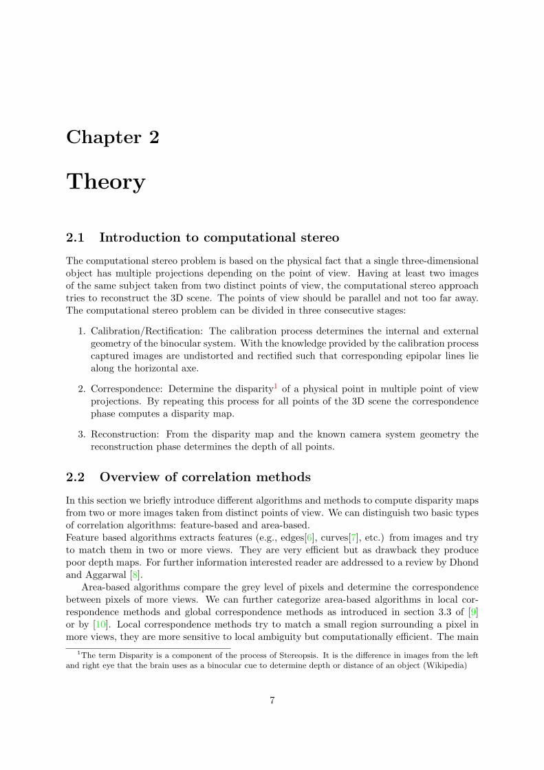
The computational stereo problem is based on the physical fact that a single three-dimensionalobject has multiple projections depending on the point of view. Having at least two imagesof the same subject taken from two distinct points of view, the computational stereo approachtries to reconstruct the 3D scene. The points of view should be parallel and not too far away.The computational stereo problem can be divided in three consecutive stages:

1. Calibration/Rectification: The calibration process determines the internal and externalgeometry of the binocular system. With the knowledge provided by the calibration processcaptured images are undistorted and rectified such that corresponding epipolar lines liealong the horizontal axe.

2. Correspondence: Determine the disparity1 of a physical point in multiple point of viewprojections. By repeating this process for all points of the 3D scene the correspondencephase computes a disparity map.

3. Reconstruction: From the disparity map and the known camera system geometry thereconstruction phase determines the depth of all points.

2.2 Overview of correlation methods

In this section we briefly introduce different algorithms and methods to compute disparity mapsfrom two or more images taken from distinct points of view. We can distinguish two basic typesof correlation algorithms: feature-based and area-based.Feature based algorithms extracts features (e.g., edges[6], curves[7], etc.) from images and tryto match them in two or more views. They are very efficient but as drawback they producepoor depth maps. For further information interested reader are addressed to a review by Dhondand Aggarwal [8].

Area-based algorithms compare the grey level of pixels and determine the correspondencebetween pixels of more views. We can further categorize area-based algorithms in local cor-respondence methods and global correspondence methods as introduced in section 3.3 of [9]or by [10]. Local correspondence methods try to match a small region surrounding a pixel inmore views, they are more sensitive to local ambiguity but computationally efficient. The main

1The term Disparity is a component of the process of Stereopsis. It is the difference in images from the leftand right eye that the brain uses as a binocular cue to determine depth or distance of an object (Wikipedia)

7

principle is to compare each pixel of the left image with all pixels of its relative epipolar lineon the right image within a certain range. The range is defined by the maximum disparitywe want to reach, the more the disparity range is high the more we can detect close objects.Using rectified images the comparison process becomes more performing, since the correlationis made by matching pixels with the same Y coordinate. To better explain how the correlationis performed, we define a pixel in a two dimensional space as a function I(x, y) returning thepixel intensity. Intensity value is an integer going from 0 to 255. There are multiple correlationmethods, the simplest we can imagine is comparing the intensity of one pixel in to the leftimage with all pixels of the right image and retain the comparison with the lowest difference.Clearly such a method will produce an arbitrary matching, since an image has multiple pixelshaving the same intensity. To diminish the ambiguity rather than comparing only two pixels attime we compare a sequence of pixels, a portion of the image called window. Multiple methodsto compute the similarity of two windows exist, and again we can distinguish more categories.Basically there are normalizing methods and not. The Sum of absolute difference (equation 2.1)or the Sum of square difference (equation 2.2) are two examples of non-normalizing methods,the cross correlation (equation 2.3) normalizes instead the comparison by subtracting the meanwindow value.

ASD(x, y) =n∑

j=0

n∑i=0

abs(I1(x + i, y + j)− I2(x + i + d, y + j)) (2.1)

SSD(x, y) =n∑

j=0

n∑i=0

(I1(x + i, y + j)− I2(x + i + d, y + j))2 (2.2)

CC(x, y) =

∑nj=0

∑ni=0[(I1(x + i, y + j)−mx).(I2(x + i + d, y + j)−my)]√∑n

j=0

∑ni=0(I1(x + i, y + j)−mx)2.

√∑nj=0

∑ni=0(I2(x + i + d, y + j)−my)2

(2.3)Where n is the window size, I1 and I2 the left and right images pixel intensities, d the disparity,mx and my are the means of the corresponding windows.

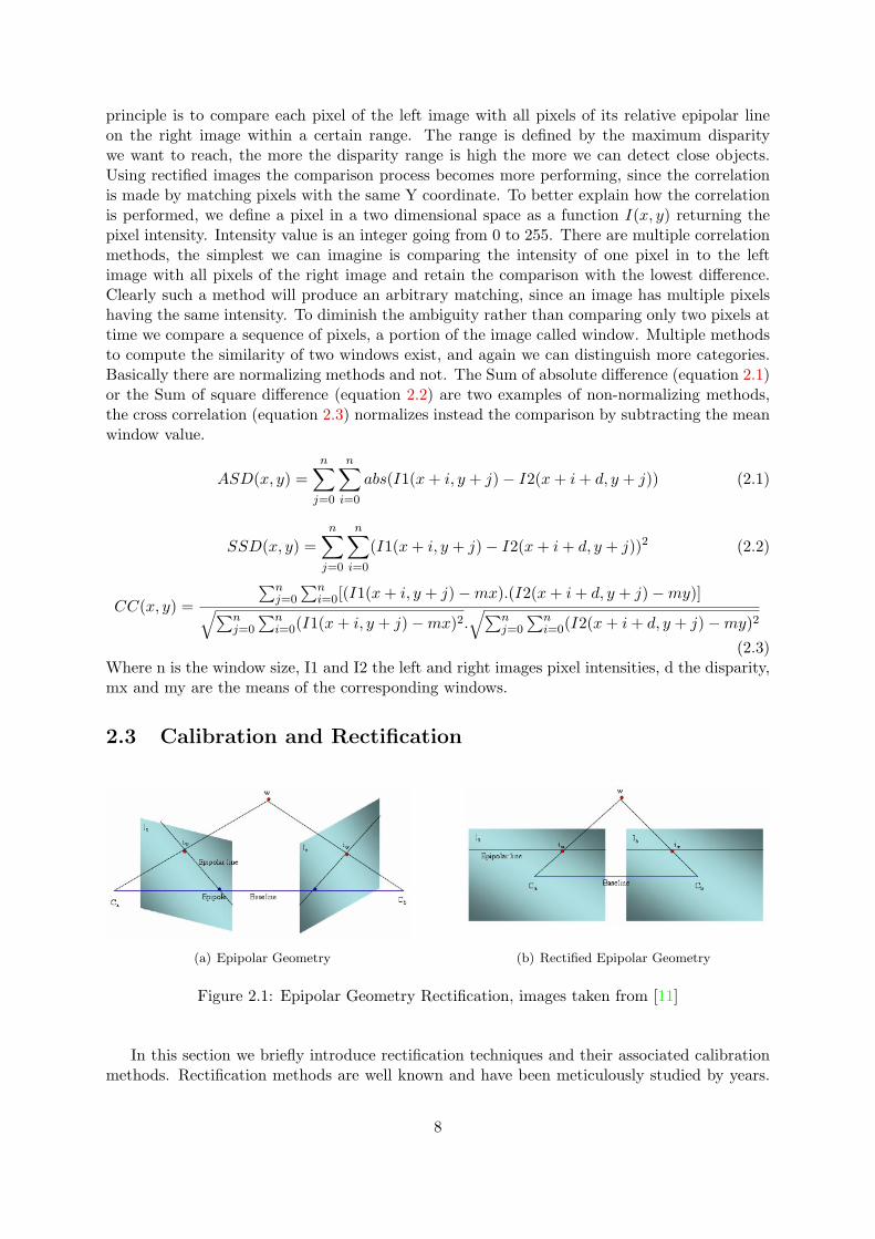
2.3 Calibration and Rectification

(a) Epipolar Geometry (b) Rectified Epipolar Geometry

Figure 2.1: Epipolar Geometry Rectification, images taken from [11]

In this section we briefly introduce rectification techniques and their associated calibrationmethods. Rectification methods are well known and have been meticulously studied by years.

8

(a) Non rectified image (b) Rectified image

Figure 2.2: Image rectification, images taken from [12]

The aim of these techniques is to adjust captured images to simplify their manipulation. Whenwe capture an image with an optical device the resulting image differs in some way from the realworld geometry. There are basically two factors that have to be adjusted in stereo applications,the image distortion and the image epipolar geometry, see figures 2.1 and 2.2.

2.3.1 Pinhole cameras

Figure 2.3: Principle of a pinhole camera (modified image taken from Wikipedia).

This section describes pinhole cameras, which is the type of camera used in our project. Thepinhole camera is the simplest projective camera that maps a three dimensional point to a twodimensional image. A pinhole camera consists of two planes, the retinal and the focal one. Onthe retinal plane the image is formed, the focal plane is parallel to the retinal one on a distanceF called focal length. A three dimensional point M from the real world is mapped to the twodimensional image via a perspective projection. Pinhole cameras are characterized by two setsof parameters. Internal or intrinsic parameters, describe the internal geometry and the opticalcharacteristics of the camera. Extrinsic or external parameters describe the camera positionand orientation on the real world. To compute a comparison between two images captured fromtwo different cameras, intrinsic and extrinsic parameters are fundamental.

2.3.2 Image distortion

Optical devices use lenses to converge images on the image sensor, therefore acquired imagesresult to be distorted since they have to pass trough a lens. Distortion factors are specific

9

to each camera and together with the focal length and the centre point they compose theintrinsic parameters of a camera. With the aid of calibration systems intrinsic parameters canbe estimated and an undistortion projective matrix is easily computed. As calibration toolreference we advise the Camera Calibration Toolbox for Matlab [13].

2.3.3 Image rectification

To rectify an image we need to apply a 2D projective transformation called homography, ob-tained from the essential or fundamental matrix. For more information on homographies, thereader is addressed to [12]. Different solutions are proposed to achieve an image rectification. Ifthe intrinsic parameters of the images (focal length, distortion, etc.) are know we can normalizeit and work with the essential matrix. Otherwise the fundamental matrix can be estimatedby calibrating the binocular system. The aim of the calibration process is to retrieve intrinsicparameters used to undistort images and extrinsic parameters used to rectify images. Bothintrinsic and extrinsic parameters compose the fundamental matrix. To provide an accurateresult two approaches are known: photogrammetric calibration and self-calibration. The firsttechnique efficiently estimates the parameters by observing a well know calibration object (cal-ibration rig) and estimating the vision system geometry. This method is adapted to stereosystems not changing their geometry during the runtime. If a stereo system using zooms orchanging its cameras angles is needed, the self-calibration technique is more adequate. Theself-calibration method does not need any calibration rig, it runs permanently but provides lessaccurate results. For further details about calibration methods the reader is addressed to [14]and [15].

10

Chapter 3

Further Analysis

3.1 Real-time correspondence algorithms

Stereo matching has been one of the most explored research area in computer vision during thelast years. There are actually many different approaches to solve this problem. S. Scharsteunand R. Szeliski [9] have well measured performances of the most common stereo correspondencealgorithms. From their work it emerges that only few correspondence approaches are suitablefor real-time1 application on a common computer architecture2. Best performances are providedby correlation based algorithms. In [16] a similar approach obtains comparable performances,but still not enough for our purposes, since at their best rate it may take a few seconds toprocess a single frame. Therefore our further works are essentially focused on correlation basedalgorithms. The first well documented real-time effort with a correlation based algorithm wasmade by the INRIA institute using a dedicated hardware [17]. In the last years many researcheshave been made to increase real-time correspondence algorithms accuracy and performance [18][19] [20] [21]. Some commercial implementations3 have reached a frame rate of more than 15fps on common personal computer architecture. We have tested the Videre Design Small VisionSystem in our labs on a 3GHz computer, and it turned out to be able to process up to 40 fps.Actually the most employed correspondence algorithms for real-time stereo matching applica-tions are correlation based. They only differ in their implementation and in some pre and postprocessing phases. In the following sections we better study correlation algorithms and crucialimage features to care about for maximizing the disparity map quality.

3.1.1 Crucial image features for correlation algorithms

Correlation based algorithms try to establish a correspondence between windows of the leftcamera image and windows of the right camera image. Different size of windows are used, thesize of the window determine the depth map resolution. As described in section 1.1 of [21]the correlation method assumes that the depth is equal for all pixels belonging to a window.Therefore small details are lost and object borders are blurred depending on the correlationwindow size. On the other hand, as shown by Nishihara and Poggio [22], the probability ofa mismatch decreases as the window size increases. Multiple correlation functions (e.g. SSD,cross correlation, etc.) measure the correspondence between windows (see section 2.2). Howeverthe quality of the disparity map for all correlation methods are strictly related to the contentof the correlation windows: the more the texture of a window differs from others, the less is

1At least 10 fps2Personal computers mounting a Pentium III processor or higher, running with at least a 700 Hz clock3Point Grey and Videre Design

11

the probability to obtain an erroneous matching. The image quality plays an important rolein algorithm precision. A picture with a good contrast, a correct luminosity, a proper colorscale and good borders definitions generates more reliable correspondences. As described by H.Hirschmuller [21] the correlation curve is not only used to determine the correspondence but alsoto determine the probability of a false matching. An other technique reduce the probabilityof having a false matching by applying the symmetric consistency check[23]. This approachcompares the place of highest similarity obtained by computing the correlation from left toright and vice versa. If the two resulting disparities coincide the consistency is respected. Byresuming we can assert that a low window texture quality (too homogeneous) is one of themain factor involved in errors generation. This facts will be taken into account to profile ourhardware requirements.

3.2 Hardware requirement for real-time stereo

As explained in the previous section, the quality of the images plays a crucial role to obtain aprecise disparity map. Different problems can affect the quality of the resulting image.

• Luminosity balance: to avoid this problem the cameras shutter time4 and the gain levelshould be variable.

• Low luminosity: to handle low luminosity situations the camera should have a highlysensitive sensor.

• Motion blur: this phenomena appears when moving the camera during the image captureprocess. To reduce this effect the shutter time should be as small as possible. A mix of goodquality lenses and cameras sensor helps to reduce the exposure time and as consequencethe shutter time.

Cameras view vectors of a stereo vision system are hardly perfectly parallel, to partially try tosettle this defect a calibration can be performed. In chapter 6 we further explore this problematicand how to minimize its troubles. Since the calibration process is made once in a while thecameras view vectors should not change. The stereo head has to be very solid, not susceptibleto vibrations or small chocks. Another important aspect is the synchronism between the twocameras. Images should be captured at the same instant. An external trigger is suitable tosolve the synchronism problem and allows us to employ the stereo head on mobile robots.

3.2.1 Commercial cameras solution

In the following section we compare some commercial cameras solutions to select a suitablecandidate for our stereo vision system. We also briefly expose some ready to use stereo heads,which directly compute depth maps, and we further investigate for wireless solutions. Unfor-tunately for our purpose, all stereo heads we found were out of size. We choose as examplesthree binocular systems produced by Point Grey, Videre Design and Focus robotics (figure 3.1).This stereo heads are delivered with their specific software. Such a ready to use product hasmultiple advantages. First user do not have to care about calibration and images rectification.Also, these stereo heads are able to produce real-time depth maps thanks to a dedicated hard-ware or stereo engines.As mentioned, we also investigated the wireless domain. Wireless is avery practical solution especially for our robots, unfortunately we did not find any applicableproduct. Basically there are two kinds of wireless cameras, analogical ones that ”broadcast”

4exposure time

12

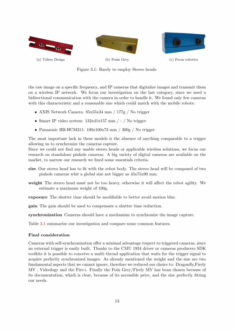
(a) Videre Design (b) Point Grey (c) Focus robotics

Figure 3.1: Raedy to employ Stereo heads.

the raw image on a specific frequency, and IP cameras that digitalize images and transmit themon a wireless IP network. We focus our investigation on the last category, since we need abidirectional communication with the camera in order to handle it. We found only few cameraswith this characteristic and a reasonable size which could match with the mobile robots:

• AXIS Network Camera: 85x55x34 mm / 177g / No trigger

• Smart IP video system: 132x41x157 mm / - / No trigger

• Panasonic BB-HCM311: 100x100x73 mm / 300g / No trigger

The most important lack in these models is the absence of anything comparable to a triggerallowing us to synchronize the cameras capture.Since we could not find any usable stereo heads or applicable wireless solutions, we focus ourresearch on standalone pinhole cameras. A big variety of digital cameras are available on themarket, to narrow our research we fixed some essentials criteria.

size Our stereo head has to fit with the robot body. The stereo head will be composed of twopinhole cameras whit a global size not bigger as 45x75x90 mm.

weight The stereo head must not be too heavy, otherwise it will affect the robot agility. Weestimate a maximum weight of 100g.

exposure The shutter time should be modifiable to better avoid motion blur.

gain The gain should be used to compensate a shutter time reduction.

synchronization Cameras should have a mechanism to synchronize the image capture.

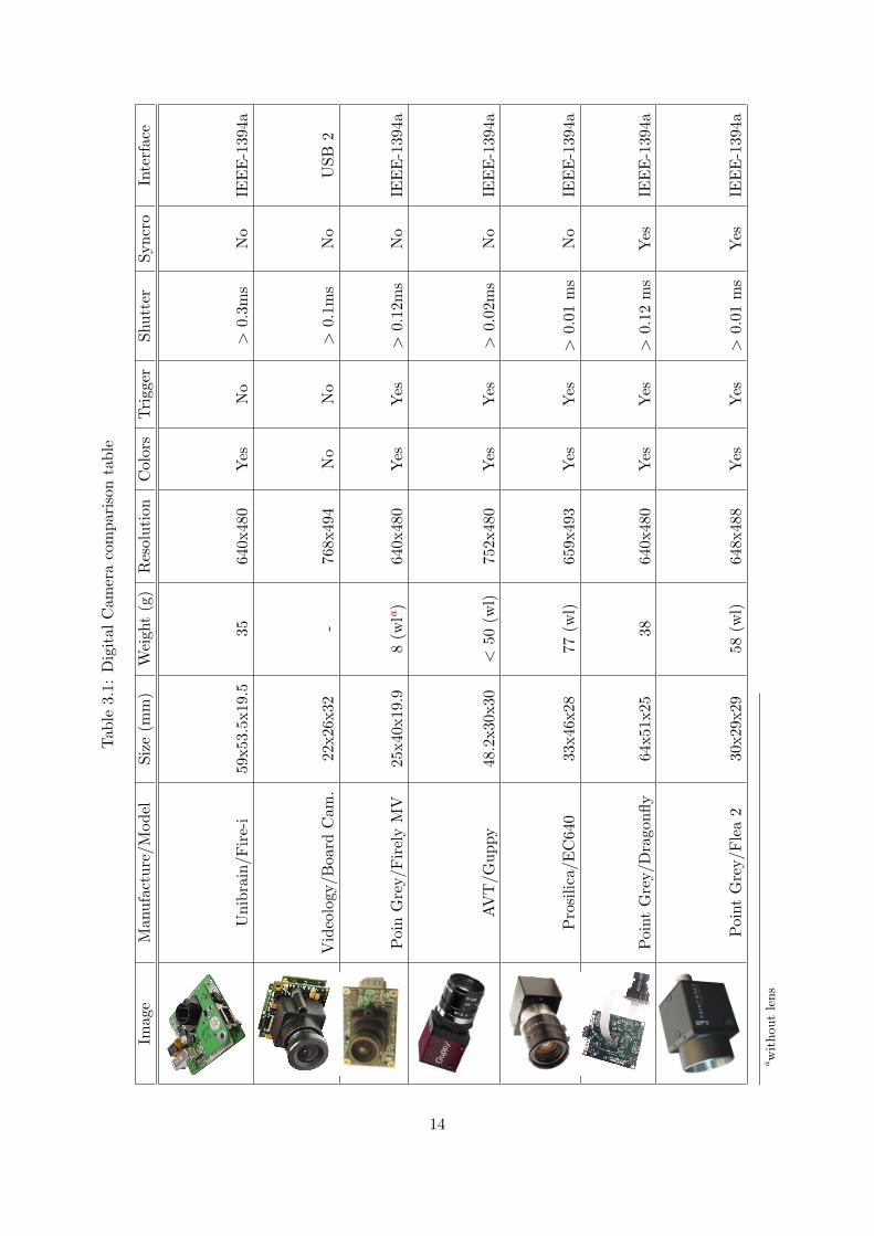
Table 3.1 summarize our investigation and compare some common features.

Final consideration

Cameras with self-synchronization offer a minimal advantage respect to triggered cameras, sincean external trigger is easily built. Thanks to the CMU 1934 driver or cameras producers SDKtoolkits it is possible to conceive a multi thread application that waits for the trigger signal toacquire perfectly synchronized images. As already mentioned the weight and the size are twofundamental aspects that we cannot ignore, therefore we reduced our choice to: Dragonfly,FirelyMV , Videology and the Fire-i. Finally the Poin Grey/Firely MV has bean chosen because ofits documentation, which is clear, because of its accessible price, and the size perfectly fittingour needs.

13

Tab

le3.

1:D

igit

alC

amer

aco

mpa

riso

nta

ble

Imag

eM

anuf

actu

re/M

odel

Size

(mm

)W

eigh

t(g

)R

esol

utio

nC

olor

sTri

gger

Shut

ter

Sync

roIn

terf

ace

Uni

brai

n/Fir

e-i

59x5

3.5x

19.5

3564

0x48

0Y

esN

o>

0.3m

sN

oIE

EE

-139

4a

Vid

eolo

gy/B

oard

Cam

.22

x26x

32-

768x

494

No

No

>0.

1ms

No

USB

2

Poi

nG

rey/

Fir

ely

MV

25x4

0x19

.98

(wla

)64

0x48

0Y

esY

es>

0.12

ms

No

IEE

E-1

394a

AV

T/G

uppy

48.2

x30x

30<

50(w

l)75

2x48

0Y

esY

es>

0.02

ms

No

IEE

E-1

394a

Pro

silic

a/E

C64

033

x46x

2877

(wl)

659x

493

Yes

Yes

>0.

01m

sN

oIE

EE

-139

4a

Poi

ntG

rey/

Dra

gonfl

y64

x51x

2538

640x

480

Yes

Yes

>0.

12m

sY

esIE

EE

-139

4a

Poi

ntG

rey/

Fle

a2

30x2

9x29

58(w

l)64

8x48

8Y

esY

es>

0.01

ms

Yes

IEE

E-1

394a

aw

ithout

lens

14

Chapter 4

Tools

In this chapter we introduce all libraries, applications and any kind of tool we conceived to helpus during the project.

4.1 Calibration Tool

Start

Grab left img

Grab right img

Detect chessboard

Detect chessboard

Both chessboard are

detected

Add point to list

Compute calib params

Is there enough points

Save to XML file Stop

Wait 10ms

Does the user accept the

image?

No or Time-out

No

Yes

No

Yes

Show Images

Draw points

on img.

Yes

Figure 4.1: Semi automated calibration work flow

We chose to conceive a semi-automated calibration tool allowing us to rapidly detect thecalibration rig and capture the images. As the aim of this project is not focused on calibrationand stereo images rectification, a big portion of our calibration system will be based on existingimplementations. The conception of a calibration system is largely influenced by the bounded

15

hardware. In our case we chose two identical cameras without zoom or any variable optics.Cameras are mounted on a rigid support so that their distance and orientations are fixed.Having a stereovision system with fixed intrinsic and extrinsic parameters allows us to takeadvantage from the photogrammetric calibration method. The Photogrammetric calibrationresult to be more precise than self calibration methods as motioned by Z. Zhang in [14]. Usinga photogrammetric method, calibration is only performed once, unless the stereovision systemis altered. Since intrinsic and extrinsic parameters do not change, they can be stored andfurther used to rectify images. This approach is less adaptive than the self-calibration one,on the other hand the photogrammetric method is more accurate, and increases the stereocomputation performance. This is possible since the calibration values are already known.Nowadays the most widely useed and evolved calibration library is the Camera calibrationToolbox for MatLab. This library is based on Zhang’s algorithm [15] and implemented byJean-Yves Bouguet. Unfortunately the Matlab version of the calibration toolbox is not flexibleenough for our purposes, therefore we took the OpenCV C++ implementation and built aroundit a semi-automated calibration application.

4.1.1 Calibration Tool Architecture

The semi-automated calibration tool is a standalone C++ application capable of computingand store on a XML file the calibration parameters. It also stores the images so that cali-bration parameters can be estimated with other applications. As second solution to estimatethe calibration parameters we used the Videre Design SVS application [24]. The calibrationusing the SVS was obtained using the images provided by our semi-automated calibration tool.The schema 4.1 illustrates the images acquisition workflow. The application is composed bythree external libraries: our synchronized frame grabber (section 4.2), the OpenCV R 1.0 andXMLParser v2.23 of Frank Vanden Berghen (a simple and small XML parser). To better allowreutilization, extension and portability of our application we chose to store calibration param-eters in a proper XML format, annex E shows an example. The innovation in our calibrationapplication is that we added a new decision layer establishing if the acquired calibration frame(image) is valid or not. Instead of taking a still picture at input we grab a video stream in whichthe calibration rig is continuously searched. The layer itself is extremely simple, but offers mul-tiple advantages. Wrong frames not containing the full calibration pattern are automaticallydropped and new ones are grabbed from the stereovision camera system. The decision layerstart acquiring images from both cameras. Once on both images (left, right) a chessboard isfound and corners are correctly detected the image acquisition stops. The user is asked to acceptor refuse the last captured image as valid. A list of accepted images is established. Once therequired numbers of images are accepted, the calibration parameters are computed and savedin to a XML file. The calibration application is especially conceived for binocular system, ourproject has a well defined configuration therefore the calibration application is not suitable forstereo vision systems with variable configuration. Although we have implemented the stereoapplication so that it can work with an arbitrary number of cameras, user needs to change aconstant value and recompile the application in order to modify the number of input cameras.

4.2 Synchronized Frames Grabber

For synchronized frames grabber we refer to an application or library able to simultaneouslygrab several frames generated by a multi-camera system. Each frame for each camera shouldbe acquired at the same instant. More precisely, the cameras sensor exposition should besynchronized, whereas no importance is given to the data transfer. A proper synchronized

16

fames grabber utility provides multiple advantages. If your stereovision system is conceived tobe displaced (e.g. your cameras are mounted on a moving robot), the cameras synchronizationis essential to determine a correct depth map. Without synchronized cameras the geometrylinking their points of view varies during time according to the cameras system displacement.Imagine that you are a robot with two cameras; now with your left camera you take a picture,you make one step forward and with your right camera you take a second picture. Your capturedimages will not correspond and the computed depth map will be wrong. A simple method toavoid this phenomenon is to ensure that all frames are captured at the same time.

4.2.1 Specification

Acquisition Thread 2

Acquisition Thread 1 Acquire

Acquire



Acquire

Acquire

Trigger Clock

TIME

Camera 1

Camera 2

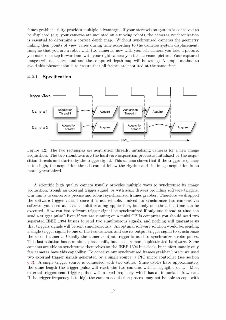
Figure 4.2: The two rectangles are acquisition threads, initializing cameras for a new imageacquisition. The two rhombuses are the hardware acquisition processes initialized by the acqui-sition threads and started by the trigger signal. This schema shows that if the trigger frequencyis too high, the acquisition threads cannot follow the rhythm and the image acquisition is nomore synchronized.

A scientific high quality camera usually provides multiple ways to synchronize its imageacquisition, trough an external trigger signal, or with some drivers providing software triggers.Our aim is to conceive a precise and robust synchronized frames grabber. Therefore we droppedthe software trigger variant since it is not reliable. Indeed, to synchronize two cameras viasoftware you need at least a multithreading application, but only one thread at time can beexecuted. How can two software trigger signal be synchronized if only one thread at time cansend a trigger pulse? Even if you are running on a multi CPUs computer you should need twoseparated IEEE 1394 busses to send two simultaneous signals, and nothing will guarantee usthat triggers signals will be sent simultaneously. An optimal software solution would be, sendinga single trigger signal to one of the two cameras and use its output trigger signal to synchronizethe second camera. Usually the camera output trigger is used to synchronize strobe pulses.This last solution has a minimal phase shift, but needs a more sophisticated hardware. Somecameras are able to synchronize themselves on the IEEE 1394 bus clock, but unfortunately onlyfew cameras have this capability. To conceive our synchronized frames grabber library we usedtwo external trigger signals generated by a single source, a PIC micro controller (see section6.3). A single trigger source is connected with two cables. Since cables have approximatelythe same length the trigger pulse will reach the two cameras with a negligible delay. Mostexternal triggers send trigger pulses with a fixed frequency, which has an important drawback.If the trigger frequency is to high the camera acquisition process may not be able to cope with

17

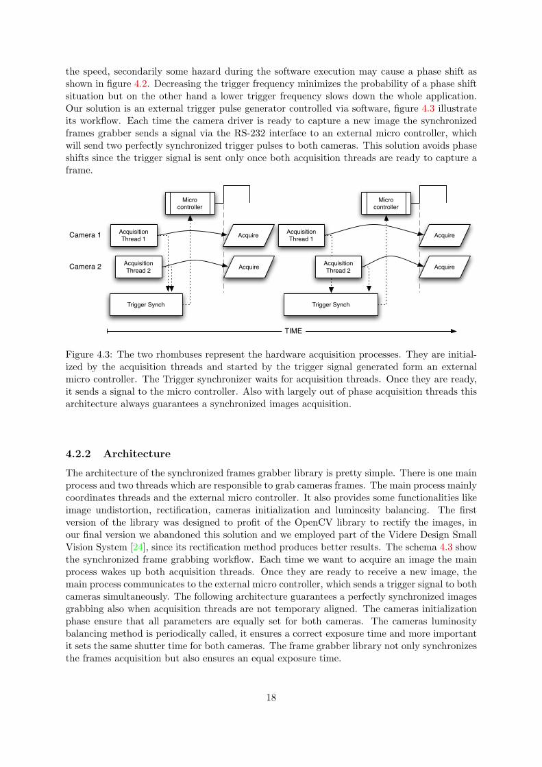
the speed, secondarily some hazard during the software execution may cause a phase shift asshown in figure 4.2. Decreasing the trigger frequency minimizes the probability of a phase shiftsituation but on the other hand a lower trigger frequency slows down the whole application.Our solution is an external trigger pulse generator controlled via software, figure 4.3 illustrateits workflow. Each time the camera driver is ready to capture a new image the synchronizedframes grabber sends a signal via the RS-232 interface to an external micro controller, whichwill send two perfectly synchronized trigger pulses to both cameras. This solution avoids phaseshifts since the trigger signal is sent only once both acquisition threads are ready to capture aframe.



Acquire

Trigger Synch

Micro controller



Acquire

Trigger Synch

Micro controller

TIME

Camera 1

Camera 2

Figure 4.3: The two rhombuses represent the hardware acquisition processes. They are initial-ized by the acquisition threads and started by the trigger signal generated form an externalmicro controller. The Trigger synchronizer waits for acquisition threads. Once they are ready,it sends a signal to the micro controller. Also with largely out of phase acquisition threads thisarchitecture always guarantees a synchronized images acquisition.

4.2.2 Architecture

The architecture of the synchronized frames grabber library is pretty simple. There is one mainprocess and two threads which are responsible to grab cameras frames. The main process mainlycoordinates threads and the external micro controller. It also provides some functionalities likeimage undistortion, rectification, cameras initialization and luminosity balancing. The firstversion of the library was designed to profit of the OpenCV library to rectify the images, inour final version we abandoned this solution and we employed part of the Videre Design SmallVision System [24], since its rectification method produces better results. The schema 4.3 showthe synchronized frame grabbing workflow. Each time we want to acquire an image the mainprocess wakes up both acquisition threads. Once they are ready to receive a new image, themain process communicates to the external micro controller, which sends a trigger signal to bothcameras simultaneously. The following architecture guarantees a perfectly synchronized imagesgrabbing also when acquisition threads are not temporary aligned. The cameras initializationphase ensure that all parameters are equally set for both cameras. The cameras luminositybalancing method is periodically called, it ensures a correct exposure time and more importantit sets the same shutter time for both cameras. The frame grabber library not only synchronizesthe frames acquisition but also ensures an equal exposure time.

18

Synchronized Frames Grabber Library

initgrabFramesgrabFramesRectifyluminosityBalance

InterfaceSynchFramesGrabber

Class implementationCMUSynchFramesGrabber

Class implementationPGRSynchFramesGrabber

CMU Driver Point Grey SDK

XML Parser

Open CV

Videre Design (SRI) SVS

Figure 4.4: The synchronized frame grabber library package structure.

4.2.3 Conception

In order to develop an extensible synchronized frames grabber library and a flexible stereo visiontool kit we defined a C++ interface. The advantage of defining such an interface is that thestereovision system makes abstaction from the employed hardware. We defined the output thata synchronized frames grabber library has to produce, the initialization method and all kind ofcommunication between the library and the employing application. For each kind of cameras,operating system or driver you want to employ a class implementing our interface has to beconceived. Therefore the binding is easily done since the stereo vision toolkit interacts withthe synchronized frames grabber library whitout caring about its specific implementation andthe type of connected hardware. As a practical example in the scope of our project we haveimplemented two classes, employing the CMU 1394 Digital Camera Driver and the Point GreyFlyCapture SDK. The CMU Driver works whit all cameras that comply with the 1394 DigitalCamera Specification, it makes of it our most portable solution. The Point Grey FlyCaptureSDK implementation is restricted to the Point Grey cameras, but it allows a better controland the acquisition of their raw image format. To demonstrate the effectiveness we made avideo (http://www.elia.ch/svs/synchDemo.avi) and extracted two significant frames to reporthere. We have over exposed the images to better emphasize the phenomena. While the videocapture we have moved a pencil in front of the cameras from left to right with a fast rhythm.Figure 4.5(a) is the result without cameras synchronization and figure 4.5(b) was obtained byactivating the cameras synchronization feature.

(a) Left and right cameras images acquired withoutcameras synchronization

(b) Left and right cameras images acquired with cam-eras synchronization

Figure 4.5: An acquisition without and with the synchronization feature

19

http://www.elia.ch/svs/synchDemo.avi

4.2.4 Remarks

During the development we lost some hours around a bug that should be located on FireFlycameras or in the CMU driver. During the initialization phase some registers are not correctlyset. To surround this problem we initialize both cameras, after that we set all parameters, wereinitialize both cameras twice but this time without reseting them to their default options.

4.3 Test and Tuning GUI

Figure 4.6: A screen shot of the Testing and Tuning GUI

To help us during the development to test our innovations and managing the correspondencealgorithm parameters in real-time, we conceived a stand alone graphical user interface. Theinterface was developed in C#, since it allows to quickly conceive and adapt the graphicaluser interface thanks to its effortless development tool, Visual Studio .NET. As our stereovision libraries are completely developed in C++ we conceived an intermediate dynamic library(dll) which is loaded by the graphical user interface. During the proceed of our project thisinterface becomes the point of conjunction between our work and the one provided by MatteoDe Giacomi [5], therefore the interface has been extended for managing some parameters of therobots behavior. The further development of this tool has been abandoned since it was replacedby a more adapted architecture, which fully integrates this project and the work provided byMatteo De Giacomi.

20

Chapter 5

Correspondence Algorithm

5.1 Introduction

0 10 20 30 40 50 60 70 80 900

50

100

150

200

250

300

Disparity

cm

Distance at Disparity

Measured dataExtrapolate data

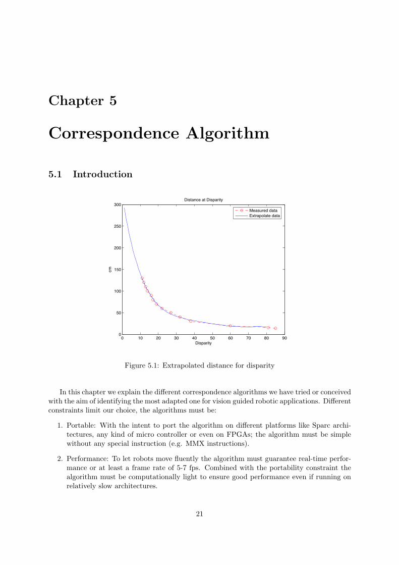
Figure 5.1: Extrapolated distance for disparity

In this chapter we explain the different correspondence algorithms we have tried or conceivedwith the aim of identifying the most adapted one for vision guided robotic applications. Differentconstraints limit our choice, the algorithms must be:

1. Portable: With the intent to port the algorithm on different platforms like Sparc archi-tectures, any kind of micro controller or even on FPGAs; the algorithm must be simplewithout any special instruction (e.g. MMX instructions).

2. Performance: To let robots move fluently the algorithm must guarantee real-time perfor-mance or at least a frame rate of 5-7 fps. Combined with the portability constraint thealgorithm must be computationally light to ensure good performance even if running onrelatively slow architectures.

21

3. Precision: To avoid obstacles a complete information about the object in front of therobot is not needed, we just want to know if there are some obstacles and their distancefrom the robot.

We can distinguish two basic types of correspondence algorithms: feature based and area basedalgorithms. This last category can be further divided into local and global correspondencemethods. A more complete description is given in chapter 2.2. Our research is addressed toarea based algorithm, since feature based ones do not generate dense depth map and have diffi-culty to match smooth surfaces. The main challenge of adopting an area based correspondencealgorithm is its computational cost. An area based algorithm produces a dense depth map,which means that for each pixel of an image the algorithm tries to find its mutual pixel onthe other views. This process is quite computationally expensive, but profiting on optimizationtechniques and by preprocessing pixels we can reach a good compromise between the depth mapdensity and its computational cost.

The final output we want to produce is slightly different from usual depth map functions.

Search the border to the right, analog to the

algorithm above.

Do the same to correct all right object borders analog

to the algorithm above.

6. Summary of the whole algorithm

The improvements, which have been suggested in the last

sections can be included into the framework of a standard

correlation algorithm. The source images are expected to be

rectified, so that the epipolar lines correspond with image

rows.

1. Pre-filtering source images as needed, using LOG. The

standard deviation ! controls smoothening.

2. Correlate using a configuration with one window, five,

nine or 25 windows as described in section 3. An opti-

mised calculation of correlation values is required for

real time applications [10]. The kind of correlation

measure needs to be chosen (e.g. SAD). Parameters

are the width and height of the correlation window cwand ch.

3. The left/right consistency check invalidates places of

uncertainty [9]. It can effectively be implemented by

temporarily storing all correlation values of all dispar-

ities for one image row.

4. The error filter can be used to reduce errors further, as

described in section 4. The threshold t f is needed as a

parameter.

5. The border correction may be used in the end to im-

prove the disparity image as described in section 5.

7. Results on real images

7.1. Experimental setup and analysis

A stereo image pair from the University of Tsukuba (figure

5) and an image of a slanted object from Szeliski and Zabih

[11] have been used for evaluation. Both are provided on

Szeliski’s web-page7. The image of the slanted object is

very simple. However, it is expected to compensate for the

lack of slanted objects in the Tsukuba images.

All disparities that are marked as invalid during the cor-

relation phase have been ignored for comparison with the

ground truth. Disparities that differ by only one from the

ground truth are considered to be still correct [11]. The

amount of errors at object borders is calculated as explained

in section 2 and shown separately.

7http://www.research.microsoft.com/szeliski/stereo/

The difference images, which are provided next to the

disparity images show the enhanced difference of disparity

and ground truth. Correct matches appear in medium gray,

while darker spots indicate that these pixels are calculated

as being further away as the ground truth states. Whereas

light spots show that those pixels are calculated as being too

close.

Figure 5: The left image and the ground truth from the Uni-

versity of Tsukuba.

The range of possible disparities has been set to 32 in all

cases. For every method, all combinations of meaningful

parameters were computed to find the best possible combi-

nation for the Tsukuba images. The horizontal and vertical

window size was usually varied between 1 and 19. The stan-

dard deviation of the LOG filter was varied in steps of 0.4

between 0.6 and 2.6. All together almost 20000 combina-

tions were computed for the Tsukuba image set, which took

several days using mainly non-optimised code.

7.2. Results of standard correlation methods

The results of the best parameter combination (i.e. which

gives the lowest error) for some standard correlation meth-

ods can be found in the first part of table 2. The MW-SAD

approach performs correlation at every disparity with nine

windows with asymmetrically shifted points of interest and

uses the best resulting value. Algorithms, which are based

on this configuration have been proposed in the literature

for improving object borders [6].

The best parameter combinations of the Tsukuba images

have been used on the slanted object images as well. Al-

most all errors occur near object borders on this simple im-

age set. This is probably due to the evenly strong texture

and the lack of any reflections, etc. It is interesting that

the slanted nature of the object, which appears as several

small depth changes, is generally well handled. However,

the weak slant is not really a challenge for correlation. The

results are not explicitely shown here, because they reflect

the same tendency as the results of the Tsukuba images, es-

pecially there ordering. However, it is a confirmation of the

qualitatively correct assessment of the evaluated methods.

The SAD correlation (figure 6) was chosen as the basis

for an evaluation of the proposed improvements. It is the

fastest in computation and shows advantages over NCC and

!"#$%%&'()*+#,+-.%+/000+1#"2*.#3+#(+4-%"%#+5(&+678-'9:5*%8'(%+;'*'#(+<46:;=>?@+

>9ABCD9?EFA9?G>?+H?AI>>+J+F>>?+!"""#

(a) Stereo image (only the left one)


algorithm above.








rows.















parameter.
























close.


versity of Tsukuba.


































!"#$%%&'()*+#,+-.%+/000+1#"2*.#3+#(+4-%"%#+5(&+678-'9:5*%8'(%+;'*'#(+<46:;=>?@+

>9ABCD9?EFA9?G>?+H?AI>>+J+F>>?+!"""#

(b) Disparity map


algorithm above.








rows.















parameter.
























close.


versity of Tsukuba.


































!"#$%%&'()*+#,+-.%+/000+1#"2*.#3+#(+4-%"%#+5(&+678-'9:5*%8'(%+;'*'#(+<46:;=>?@+

>9ABCD9?EFA9?G>?+H?AI>>+J+F>>?+!"""#

200

200

200

150

200

150 50

50

150

50 100 100 100

50 20

200 200 200 200

200100

(c) Depth grid

Figure 5.2: From source to output.

Our library is conceived for robot vision guided applications, therefore it do not return thedepth value for each pixel but the median value at each sector. The field view is decomposed inmultiple sectors as showed in figure 5.2(b). From the rectified input images to the depth gridoutput the algorithm passes trough three consecutive phases:

1. The correspondence phase is the heaviest process, it finds the correlation between thepixels of the two images (left/right) and produces the disparity map, figure 5.2(c).

2. From the disparity map, a disparity median grid is easily computed by estimating thedisparity median value for each sector.

3. The depth values of each sector is calculated form the disparity median value thanks toa conversion function, obtained by calibrating our stereo vision system. To calibrate thestereo vision system we have placed a target at a distance of 130 cm and we saved thecomputed disparity every 10 cm while approaching the target. These measures allow usto establish a relation between the real obstacle distances (cm) and their correspondingdisparity values (0 to 80 for our algorithm). This relation takes the form of a conversionfunction computed by interpolating the performed measures in order to obtain a polyno-mial function. This allows us to extrapolate the missing values. Figure 5.1 illustrates theinterpolated conversion curve.

22

Measures and MatLab code to interpolate the measures and extrapolate the missing values areavailable in annex B. Each measure is the median of the values of at least three sectors wherethe target was present.

In the next sections of this chapter we present five correspondence algorithms. We will de-scribe our effort and the road map needed to find out the algorithm which we believe to be themost adapted for vision guided robotics applications.

5.2 Dynamic Programming Algorithm

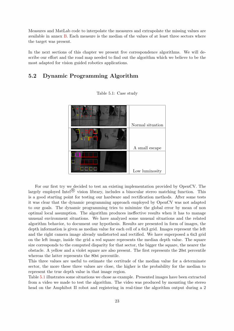
Table 5.1: Case study

Normal situation

A small escape

Low luminosity

For our first try we decided to test an existing implementation provided by OpenCV. Thelargely employed Intel R© vision library, includes a binocular stereo matching function. Thisis a good starting point for testing our hardware and rectification methods. After some testsit was clear that the dynamic programming approach employed by OpenCV was not adaptedto our goals. The dynamic programming tries to minimize the global error by mean of nonoptimal local assumption. The algorithm produces ineffective results when it has to manageunusual environment situations. We have analyzed some unusual situations and the relatedalgorithm behavior, to document our hypothesis. Results are presented in form of images, thedepth information is given as median value for each cell of a 6x3 grid. Images represent the leftand the right camera image already undistorted and rectified. We have superposed a 6x3 gridon the left image, inside the grid a red square represents the median depth value. The squaresize corresponds to the computed disparity for that sector, the bigger the square, the nearer theobstacle. A yellow and a violet square are also present. The first represents the 20st percentilewhereas the latter represents the 80st percentile.This three values are useful to estimate the certitude of the median value for a determinatesector, the more these three values are close, the higher is the probability for the median torepresent the true depth value in that image region.Table 5.1 illustrates some situations we chose as example. Presented images have been extractedfrom a video we made to test the algorithm. The video was produced by mounting the stereohead on the Amphibot II robot and registering in real-time the algorithm output during a 2

23

minute robot promenade. Afterwards we extracted some typical and atypical situations fromthe video to examine the algorithm behavior. The first image (Normal situation) shows what weexpect to obtain. The following two examples are to demonstrate the bad assumptions whichthe algorithm mades to minimize the global error. In the first case a small escape door on theright is totally missed. In the second case we notice that an homogeneous texture produce acompletely wrong depth map. As conclusion of this test (whose results are partially presentedon this report) we decided to abandon the OpenCV implementation and start developing ourown correspondence algorithm. More case studies are available in appendix A.

5.3 Block matching Algorithm

Block matching algorithms establish the disparity for a given block called window, by analyzingthe result of the correlation function. The matching model is simple. Unlike the dynamicprogramming the decision is taken independently from any higher level information, since theonly relevant data are relative to the current window. For every window a similarity value isreturned for all disparities. These values are produced by the correlation function. The numberof maximal disparities to check is predefined. The more the maximal disparity value is highthe more the computation is slowed down, whereas the more this value is small the more theminimal detected distance is limited. In our case we fixed the maximal disparity to 80 pixels,which with our stereo vision system allows us to detect objects from a minimal distance of 15cm. As correlation function we chose the Sum of Square Differences:

SSD(x) =n∑

i=0

(I1(x + i)− I2(x + i + d))2 (5.1)

The SSD is the second lightest function in terms of computational cost, but is more discriminantthan the lass expensive one, the Absolute Sum of Differences. We should point out that ourSSD function is one-dimensional, which allows us to better optimize the code. As consequencethe comparison window has a one-dimension as well. In chapter 7 we compare our algorithmwith the Videre Design SVS [24], and we observed the a one-dimensional window does notcompromise the algorithm quality. The Small Vision System is an efficient implementation ofthe SRI stereo algorithm, that was recently purchased by the Videre Design company. The SRIstereo algorithm is hold secret but we know that it adopt a block matching technique mergingmatching at multiple resolutions. Thanks to some filters they are able to increase the algorithmreliability. A good correlation function itself is not enough to establish a correct correspondence,therefore we decide to enrich our matching model by adding a cost function. The cost functiontransforms linearly the computed correlation values by penalize high disparity values. This isdone since an image window representing close objects is less probable.

cost(x) = x ∗ (d ∗ 0.16 + 1.0) (5.2)

where d is the actual disparity and x is the SSD value obtained for that d. We have empiricallychose 0.16 as cost factor since we have observed a maximal increase of the disparity mapquality. For our first versions as consistency test we adopted the symmetric check [23][25]. Thetest defines as valid a match obtaining the same correlation for a given pixel by computing thecorrespondence from the left to the right image and vice versa.

5.3.1 Stereoscopic Machine Vision Algo v.1

Our correspondence algorithm is based on the simplest correspondence model, a scanningmethod and a one to one correlation function. We compute the correlation between one window

24

of the left image and multiple windows of the right one. The correspondence having the highestsimilarity score is selected. We believe that for vision guided applications using the most simplecorrespondence model is gaining, since the noise is specific to each pixel (not distributed overa scan line, etc.). The output is a raw depth grid (presented in section 5.1) where each cellis the median value of a region of pixels. Noisy pixels can therefore be dropped and only theones having an high confidence value can be taken into account. The number of pixels selectedto compute the median determines the confidence measure. If the number of dropped pixelsfor a specific region is too hight the depth value will not be representative. Behind a certainthreshold we state the depth value is unknown. The threshold value has been empirically fixedat 20%. No tests has been made to determinate its optimal value since the algorithm v.1 is adraft.The correlation function we adopted is the Sum of Square Differences already introduced atthe begin of this chapter. The scanning method is the same of all area-based correspondencealgorithms. For each pixel of the left image the similarity is tested by computing the corre-spondence with each pixel of the right image being on the same Y coordinate and within arange defined by the maximal disparity. For further details about the correlation functions andscanning methods see section 2.2.

Vertical Smoothing

px

px

Stereo Image Pixels Intensities Differences (median value: 454)

50 100 150 200 250 300

50

100

150

200 Lower

Higher

(a) SSDPI without smoothing, median value 454

px

px

Stereo Image Pixels Intensities Differences (median value: 397)

50 100 150 200 250 300

50

100

150

200 Lower

Higher

(b) SSDPI with smoothing, median value 397

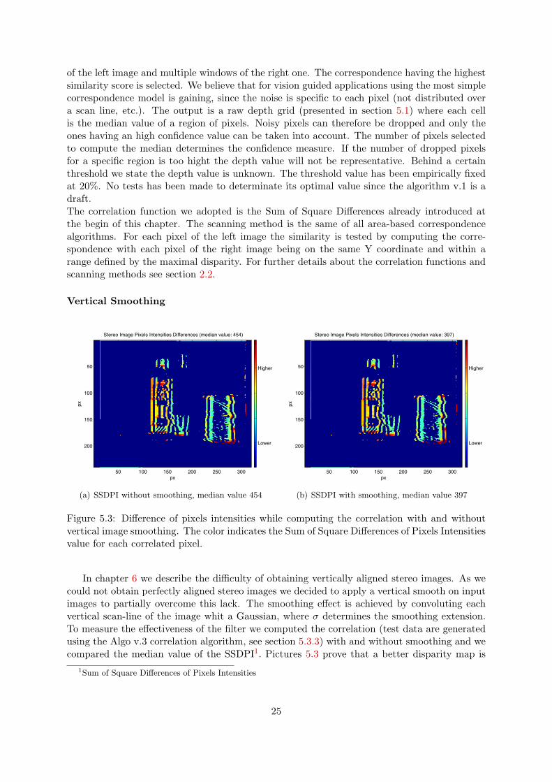
Figure 5.3: Difference of pixels intensities while computing the correlation with and withoutvertical image smoothing. The color indicates the Sum of Square Differences of Pixels Intensitiesvalue for each correlated pixel.

In chapter 6 we describe the difficulty of obtaining vertically aligned stereo images. As wecould not obtain perfectly aligned stereo images we decided to apply a vertical smooth on inputimages to partially overcome this lack. The smoothing effect is achieved by convoluting eachvertical scan-line of the image whit a Gaussian, where σ determines the smoothing extension.To measure the effectiveness of the filter we computed the correlation (test data are generatedusing the Algo v.3 correlation algorithm, see section 5.3.3) with and without smoothing and wecompared the median value of the SSDPI1. Pictures 5.3 prove that a better disparity map is

1Sum of Square Differences of Pixels Intensities

25

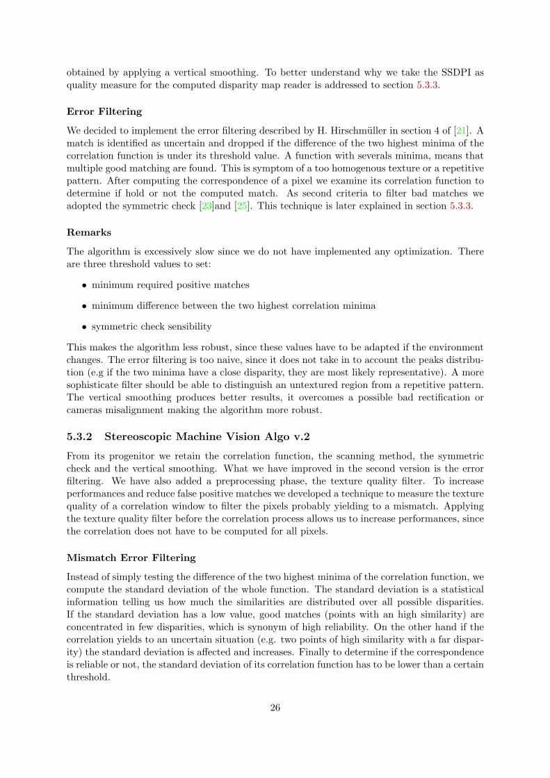
obtained by applying a vertical smoothing. To better understand why we take the SSDPI asquality measure for the computed disparity map reader is addressed to section 5.3.3.

Error Filtering

We decided to implement the error filtering described by H. Hirschmuller in section 4 of [21]. Amatch is identified as uncertain and dropped if the difference of the two highest minima of thecorrelation function is under its threshold value. A function with severals minima, means thatmultiple good matching are found. This is symptom of a too homogenous texture or a repetitivepattern. After computing the correspondence of a pixel we examine its correlation function todetermine if hold or not the computed match. As second criteria to filter bad matches weadopted the symmetric check [23]and [25]. This technique is later explained in section 5.3.3.

Remarks

The algorithm is excessively slow since we do not have implemented any optimization. Thereare three threshold values to set:

• minimum required positive matches

• minimum difference between the two highest correlation minima

• symmetric check sensibility

This makes the algorithm less robust, since these values have to be adapted if the environmentchanges. The error filtering is too naive, since it does not take in to account the peaks distribu-tion (e.g if the two minima have a close disparity, they are most likely representative). A moresophisticate filter should be able to distinguish an untextured region from a repetitive pattern.The vertical smoothing produces better results, it overcomes a possible bad rectification orcameras misalignment making the algorithm more robust.


From its progenitor we retain the correlation function, the scanning method, the symmetriccheck and the vertical smoothing. What we have improved in the second version is the errorfiltering. We have also added a preprocessing phase, the texture quality filter. To increaseperformances and reduce false positive matches we developed a technique to measure the texturequality of a correlation window to filter the pixels probably yielding to a mismatch. Applyingthe texture quality filter before the correlation process allows us to increase performances, sincethe correlation does not have to be computed for all pixels.

Mismatch Error Filtering

Instead of simply testing the difference of the two highest minima of the correlation function, wecompute the standard deviation of the whole function. The standard deviation is a statisticalinformation telling us how much the similarities are distributed over all possible disparities.If the standard deviation has a low value, good matches (points with an high similarity) areconcentrated in few disparities, which is synonym of high reliability. On the other hand if thecorrelation yields to an uncertain situation (e.g. two points of high similarity with a far dispar-ity) the standard deviation is affected and increases. Finally to determine if the correspondenceis reliable or not, the standard deviation of its correlation function has to be lower than a certainthreshold.

26

Texture Quality Filter

The correlation process computes the similarity between two windows by taking into accountthe difference of their pixels intensities or other factors depending on the correlation functionit self. There are multiple correspondence functions e.g. cross correlation, absolute sum ofdifference, sum of square difference and so on. Anyway all these functions have a commonpeculiarity, the more a window content differs from other ones the more the resulting differencewill be marked. This trivial observation leads us to the following question: what happensif we try to compute the disparity of an image region with an homogeneous texture (e.g. acompletely white region)? The computed disparity will tend to be wrong, because the windowsintensities differences are not sufficient to discriminate the correct match from other ones. Theinnovation we propose is to preprocess the comparison windows to skip those not having asufficiently heterogeneous texture, instead of computing the correlation for each pixel droppingthose not producing a discriminant intensities differences. Like for the mismatch error filtering,we use the standard deviation as confidence measure, where the window pixels intensities is thefunction. To establish if a window is sufficiently textured the standard deviation of its pixelsintensities is computed. An homogeneous window contains pixels with about the same intensity,therefore the standard deviation results lower comparing to a heterogeneous window. Only thewindows having a standard deviation higher than a certain threshold will be taken into accountto compute the correspondence.

Remarks

The texture quality filter is a good solution to minimize the computational cost since it allowsto skip the windows probably yielding to a mismatch. Unfortunately the standard deviationis not a good criteria to filter the untextured windows since it is influenced by the scene lumi-nosity. If the ambient illumination decreases also the standard deviation value will decrease byconsequence. Therefore the threshold has to be readjusted. The mismatch error filtering resultsto be redundant, the texture quality filter already drops those windows yielding to a mismatch.By precisely tuning the texture quality filter threshold, the mismatch error filtering is almostuseless.A second problem we noted is that the symmetric check error filtering has some troubles whenthe obstacle is too close to the cameras, since the points of view are too different.


Stereoscopic Machine Vision Algo v.3 is our final result, it focalizes all our effort to find themost adapted stereo algorithm for vision guided robotic applications. To reach the highestrobustness degree we retained all valid solutions and exciting innovations we found during thisproject. The correspondence model has not changed, to determinate a match we still use theSSD as a correlation function combined with the linear cost transformation.Otherwise the Stereoscopic Machine Vision Algo v.3 largely differs form its predecessors, itwas conceived to be fast on any architecture (like its previous versions) and extremely robustto the environment transformations. To achieve the first objective we adapted the texturequality filter technique introduced in version 2, which allows to ignore those pixels probablyyielding to a mismatch. The second objective, the robustness, was achieved by modifying thefiltering technique which is now fewer influenced by the scene luminosity. We also slightlyadapted the correlation process in the way that it was able to manage dysfunctional behavior(e.g. misaligned cameras view vectors). The most important difference in comparison to itspredecessors is that the Stereoscopic Machine Vision Algo v.3 does not use the symmetric

27

validity test proposed by Pascal Fua [23][25], since it doubles the computational cost. To coverthe lack we propose an alternative validity test which partially allows to detect occlusions andpossible mismatches. Next in this section we will describe the new texture quality filter, the newvalidity test, modifications we made to the correspondence process and the code optimizations.

Texture Quality Filter

!! !" !# !$ % $ # " !

!%&'

!%&%(

%

%&%(

%&'

%&'(

)

*

+,--./.01.23-245677,50

!! !" !# !$ % $ # " !%

%&%'

%&(

%&('

%&$

%&$'

)

*+,-./01234565.7./.+-

869--.6,-

!1:1(&#

!1:1;

!1:1#&"

Figure 5.4: Difference of Gaussian functions.

For the third version we abandoned the standard deviation as measure of the texture quality.This because of its proportionally dependence of the pixels intensity average and the consequentneed to adjust its threshold. To substitute the standard deviation as texture quality measurewe adopted a method usually employed to discover the points of interests, the difference-of-Gaussian.To determine if a pixel resides in a textured image zone, we convolute the window surroundingthe pixel with two difference-of-Gaussian functions at a different scale. The firs scale is moresensible on shrunken intensity variations. It returns higher values if there is a significant pixelsintensity variation concentrated in the proximity of the window center. The second difference-of-Gausian function has a larger scale (bigger σ), therefore it produces higher values if thepixels intensities are more homogeneous. The function sensibility depends from the two chosenσ values used to produce the Gaussians and they difference. An initial σ value is chosenand increased by a constant factor to determine the higher scales. David G. Lowe in [26]has demonstrated that if the σ values used to produce multiple scales of difference-of-Gausianfunctions are increased by a constant factor there is no need to normalize they result values.To define our two difference-of-Gausian functions we have chosen an initial σ and an incrementfactor ∆, from this two parameters we have obtained three Gaussian with they respective σvalues equal to: σ, σ + ∆ , σ + 2∆ . From this three Gaussian we produce two difference-of-Gausian functions by subtracting the two nearer Gaussian functions, like illustrated by figure5.4. The convolution kernel size depends of the Difference-of-Gaussian domain.The main advantage using the difference-of-Gaussian as texture heterogeneity measure is thatit is less influenced by the pixels intensity average. This is explained by the fact that thedecreasing of the pixels intensity average affects both scales. We provide in annex C a MatLabcode to generate a .h file which contains the constant values used in our library code.Figure 5.5 illustrate an example of the image filtering output, we have extracted a pixels rowfrom an image and identified those regions having a too homogeneous texture. The image was

28

0 20 40 60 80 100 120 140 160 180 200 2200

50

100

150

200

250

x (coordonate)

y (p

ixel in

tens

ity)

One pixels row of a grey scale image

0 20 40 60 80 100 120 140 160 180 200 2200

0.5

1

1.5

2

2.5

3

x (coordonate)

scal

e

Difference of Gaussian scale selection

Initial sigma: 0.4, scale factor: 3.35, kernel size 24px

Figure 5.5: Texture quality filtering results of an image row. A window of 24 pixels is convo-luted with two difference-of-Gaussian functions at a different scale. The scale producing thehighest value is taken for that coordinate. Scale 2 identify those image regions which has a toohomogeneous or smoothed texture.

produced using the MatLab code in annex D.

Validity Test

The aim of the validity test is to identify and drop those pixel correlations which we estimate tobe wrong. A well known and largely exploited validity test is the symmetric consistency check[23][25]. It identifies as valid a match that has the same disparity values when computing thecorrelation from left to right and vice versa. We will show that the symmetric check is not themost adapted validity test for our needs. The main advantage of the symmetric consistencycheck is to identify occluded regions and improve the objects edges precision. This feature isnot essential since, as our final output is a raw depth grid, we do not need to compute a precisepixel correlation. We decided not to adopt the symmetric consistency validity test becauseof its drawbacks which are more important compared to the advantages that it provides. Thesymmetric test is computationally expensive since we need to compute the correlation twice. Thesecond important disadvantage is that the symmetric consistency check rejects the correlatedregions which do not exactly correspond in both images (left, right) e.g. occluded regions. Thisbehavior is acceptable, even correct, if your goal is to establish a precise depth map, not if

29

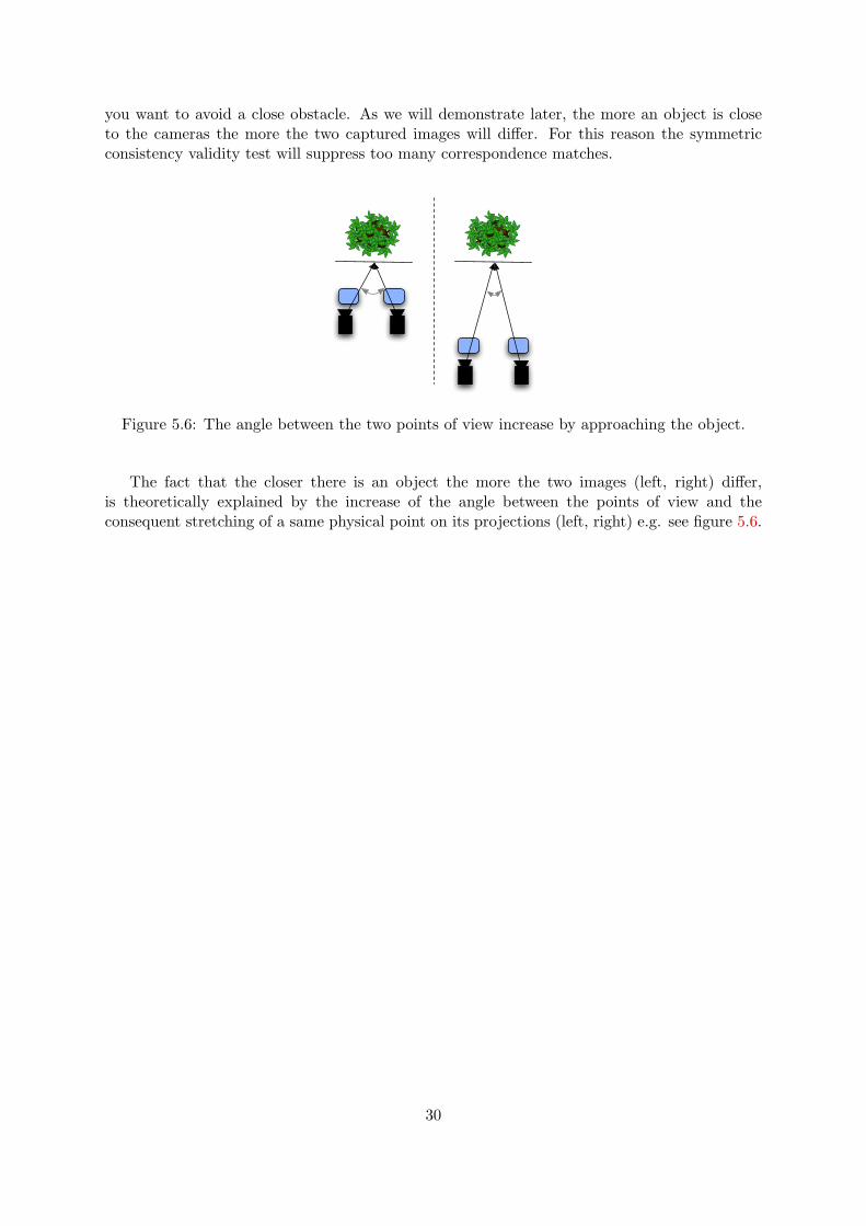
you want to avoid a close obstacle. As we will demonstrate later, the more an object is closeto the cameras the more the two captured images will differ. For this reason the symmetricconsistency validity test will suppress too many correspondence matches.

Figure 5.6: The angle between the two points of view increase by approaching the object.

The fact that the closer there is an object the more the two images (left, right) differ,is theoretically explained by the increase of the angle between the points of view and theconsequent stretching of a same physical point on its projections (left, right) e.g. see figure 5.6.

30

px

pxStereo Image Pixels Intensities Differences (mean: 8 median: 7.5)

50 100 150 200 250 300

50

100

150

200 Lower

Higher

(a) A PCI card close to cameras.

px

px

Stereo Image Pixels Intensities Differences (mean: 6.6 median: 6)

50 100 150 200 250 300

50

100

150

200 Lower

Higher

(b) The same PCI cars more distant.

Figure 5.7: Comparison between two stereo scene with the same subject at different distances.(The color indicate the SSDPI value for each correlated pixel) Lenses distortion induce toincrease the SSDPI value on image edges.

As already explained in previous section 5.3 to establish the correlation between pixels of theleft image and those of the right one, we adopted the Sum of Square Difference as correlationfunction:

SSD(x) =n∑

i=0

(I1(x + i)− I2(x + i + d))2

where n is the window size, d is the disparity and I(x) the intensity of pixel x. Once the bestcorrespondence is found we store the corresponding SSD value as a matching confidence mea-sure. More precisely each match has its own Sum of Square Difference of Pixels Intensitiesvalue, which in the following of this report we refer as SSDPI.To demonstrate in practice that the closer there is an object the more the two images differ, wechosen two scenarios. We taken an object and we computed the correlation once grabbing theimages close to the object and once far away. Then we plotted the computed SSDPI for the twoscenarios. If the two images (left, right) are exactly equal all correlated pixels will have a SSDPIvalue equal to zero, the more the two images differ the more the SSDPI value will increase. Inour scale the SSDPI goes from 0 to 12 (12 is the log of the maximum SSDPI we obtained forthat experience). Figure 5.7 shows how the SSDPI median and mean value is higher for closerobjects.To overcome this problematic we propose a new validity test which identifies as valid the corre-lations that have the SSDPI2 value lower than a dynamic threshold. The threshold is computedby trying to correlate the left image with it self and choosing the minimum SSDPI as reference.Consequently the threshold will be higher (less discriminant) for textured zones and lower inproximity of homogenous regions. An other advantage of fixing a threshold is that we canpartially filter arbitrary matches like occluded regions. Our validity test is less discriminate inpresence of close objects as our measures will prove.To measure the efficacy of our method we computed the correlation of a scene containing a closeobject, then we plotted the SSDPI value for all dropped correlation by the symmetric check andby the self check validity test. Figure 5.8 shows the test configuration and the obtained depth

2Sum of Square Difference of Pixels Intensities

31

(a) The left image, Matteo’s hand. (b) After texture quality filtering.

(c) Depth map. (d) The raw depth output. The red squares indicate theproximity.

Figure 5.8: This is the experience configuration we used to compare the self check and thesymmetric consistency validity test. The comparison is made on figure 5.9.

map. Figure 5.9 illustrate the comparison between the symmetric consistency check and the selfcheck validity test. The symmetric consistency check dropped the 55% of total correlated pixels,our method dropped 35% of total correlations and both methods has produced a comparablemean and median SSDPI value.

Back checking

Do to the difficulty to perfectly align our stereo vision system cameras view vectors we haveintroduced a validity test that usually is not required. The view vectors of our cameras hori-zontally cross they self after a certain distance (> 2.5m). Whit an hypothetic perfect hardwareand vision system resolution the disparity zero correspond to the infinite distance. The imagerectification is not able to completely correct a miss alignment, this subject is discussed in 6.1.In our case the disparity zero is already achieved after about two meters, limiting the maximalmeasurable distance to that value. To overcome this problem our algorithm as an initial dis-parity that cold be negative. If during a post processing phase a negative disparity is found,

32

px

px

Dropped Matches Using Symmetric!Check (dropped px: 52%)

50 100 150 200 250 300

50

100

150

200 Lower

Higher

px

px

After Filtering Remaining Matches (mean: 5.5 median: 4.8675 diff. of intensities value)

50 100 150 200 250 300

50

100

150

200 Lower

Higher

(a)

px

px

Dropped Matches Using Self!Check (dropped px: 35%)

50 100 150 200 250 300

50

100

150

200 Lower

Higher

px

px

After Filtering Remaining Matches (mean: 5.5 median: 5.1591 diff. of intensities value)

50 100 150 200 250 300

50

100

150

200 Lower

Higher

(b)

Figure 5.9: Comparison between the symmetric consistency validity test and the self checkvalidity test. (The color indicate the SSDPI value for each correlated pixel).

it means that that image region is behind the cameras view vectors crossing distance. Sucha situation is corrected by assigning the maximal disparity to all matches having a negativedisparity. Please note that miss cameras alignment was solve with our second prototype ofcameras support, the back checking test becomes useless and has been disabled.

Optimization

Code optimization is inspired by [17] section 2.2.6, when computing the correspondence betweento windows, all correlation values for each different disparity are stored in a table. Since the nextwindow to compare is shifted by one pixel on the left the already computed correlation valuescan be taken and slightly adjusted. The square difference of the pixel before the actual windowfor all disparities has to be added, and the square difference of the last pixel of the window forall disparities has to be subtracted. The explanation is tricky to understand, interested reader isaddressed to [17] or picture 5.10 could provides a further example. This optimization techniqueis only partially applicable to our algorithm, since the texture quality filter drops pixels. We

33

Figure 5.10: In this picture we represent a region of the left image. For one disparity the greenrectangle is the SSD for a window, at the same disparity the yellow rectangle is the SSD ofthe window shifted by one pixel. The SSD value of the yellow window has not to be fullyrecomputed, it is the SSD value of the green window minus the red square SSD value plus theblue ones.

can adopt it only when a group of consecutive windows pass trough the texture quality filter.


0 500 1000 1500 2000 25000

5

10

15

20

25Hashing distribution

hashing values

num

ber o

f ele

men

ts

Figure 5.11: The graph shows the number of elements per hash value of a hash table where allwindows of an image has been stored.

Our fourth version is just a feasibility test. We completely dropped the scanning methodand we tried a new approach. In stand of comparing a window rising from the left image withall right windows with the same Y coordinate, we put all left windows in a hash table. Onceall left image windows are in the hash table the algorithm scan the right image and step bystep it compute the hash value of the right windows to search in the hash table all possiblecorrespondences. All windows with a similar hash values are compared and only that havinga close coordinate are taken in account to compute the SSD. Our hash function is simply thesum of the pixels intensities which is not an optimal distribution function since its depend ofthe input image. In a optimal situation (not too dark, not too clear, a full textured image) thewindows distribution over the hash indexes is pretty good balance as shown in graph 5.11. Twowindows with the same sum of pixels intensities are not necessarily equal but two window witha too different sum will hardly represent the same thing. If we want to have a tolerance of 5%on each pixel where the window size is 1x9 and the intensities values goes from 0 to 255 the sumvary between ± 150. With a tolerance of 5%, 300 indexes of the hash tables has to be visitedto search a possible matching. Each index of the has table has in mean 6 elements, which make

34

1800 window to compare, this number further decrease since statistically only the 20% of thatwindows are in the proximity of the window to compare. Finally about 360 SSD comparisonare made. This algorithm makes four time more correspondences computation in comparison toits predecessors, but it is highly more robust since it does not need rectified images or perfectlyaligned cameras view vectors. We do not have further investigate on this algorithm, we onlyexpose our idea on this report as a possible solution to handle bad quality input images.

35

Chapter 6

Stereo Head (Hardware)

As stereo optic for our robots Amphibot II [1, 2] and the Salamandra Robotica [3] we couldnot use any existing solution as they do not fit with the robots size. A research to find themost adapted stereo vision hardware was made, results are exposed in section 3.2.1. We choseto couple two Firely MV PointGrey cameras and to build our own physic support to bind themtogether. The stability and the precision of the physic support plays a crucial role, since withouta correct images alignment the correspondence algorithm we employ would not work. In chapter5 we present multiple correspondence algorithms, our last version is a robust method which donot need a perfectly aligned optic support, unfortunately its drawbacks make of it not theoptimal solution. Managing bad aligned images increase the stereo matching incertitude andits computational cost, therefore we invested more time to conceive a reliable cameras supportallowing us to adopt a simpler correspondence algorithm.

6.1 Cameras and they Support

Figure 6.1: Cameras supports build with a RF-4 plate

Alessandro Crespi helps us conceiving our first cameras support and lending us his devel-opment card to generate the trigger signal. To reach a satisfying reliability we passed troughmore prototypes. The first try was made of a RF-41 plate, we cuted and we perforated byhand, cameras was fixed trough 8 crews, figure 6.1. When we conceived our first support we un-derestimate the importance of a correct cameras alignment, and unfortunately our hand madecameras support was too imprecise. If the view vectors of the cameras are not parallel on they axe the correspondence is not feasible, since the images are not vertically aligned and the

1FR-4 is a resin system material used for making printed circuit board.

36

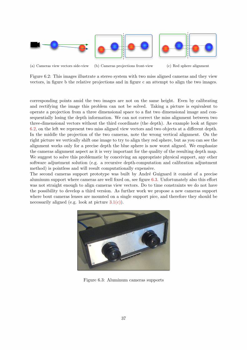
(a) Cameras view vectors side-view (b) Cameras projections front-view (c) Red sphere alignment

Figure 6.2: This images illustrate a stereo system with two miss aligned cameras and they viewvectors, in figure b the relative projections and in figure c an attempt to align the two images.

corresponding points amid the two images are not on the same height. Even by calibratingand rectifying the image this problem can not be solved. Taking a picture is equivalent tooperate a projection from a three dimensional space to a flat two dimensional image and con-sequentially losing the depth information. We can not correct the miss alignment between twothree-dimensional vectors without the third coordinate (the depth). As example look at figure6.2, on the left we represent two miss aligned view vectors and two objects at a different depth.In the middle the projection of the two cameras, note the wrong vertical alignment. On theright picture we vertically shift one image to try to align they red sphere, but as you can see thealignment works only for a precise depth the blue sphere is now worst aligned. We emphasizethe cameras alignment aspect as it is very important for the quality of the resulting depth map.We suggest to solve this problematic by conceiving an appropriate physical support, any othersoftware adjustment solution (e.g. a recursive depth-computation and calibration adjustmentmethod) is pointless and will result computationally expensive.The second cameras support prototype was built by Andre Guignard it consist of a precisealuminum support where cameras are well fixed on, see figure 6.3. Unfortunately also this effortwas not straight enough to align cameras view vectors. Do to time constraints we do not havethe possibility to develop a third version. As further work we propose a new cameras supportwhere bout cameras lenses are mounted on a single support pice, and therefore they should benecessarily aligned (e.g. look at picture 3.1(c)).

Figure 6.3: Aluminum cameras supports

37

6.2 Lenses

Figure 6.4: View angle with 32◦ lenses and 54◦

FireFly MV cameras are delivered with a 32◦ angle of view lenses, which is wide not enoughfor our robots to move fluently in their environment. We have replaced the original lenses withtwo Boowon BW38B-1000 lenses (kindly offered by Peter Kim, Boowon sales division). Thisnew lenses have a 52◦ angle of view, which at a distance of 20 cm approximatively increase thefield view of about 57%, see figure 6.4.

6.3 External Trigger

To generate the trigger pulse we employed a PIC18F2580 micro-controller coupled whit a RS232transceiver, they are mounted on printed circuit developed by Alessandro Crespi. We pro-grammed the micro-controller to catch the incoming-data interrupt generated by the integratedUART2. Each time we send some data from the PC to the micro-controller trough the RS232interface an interrupt is triggered. The interrupt is catch by the micro-controller which fires atrigger pulse to the cameras trough one of its I/O ports. The C code of the micro-controlleris available on annex F. The printed circuit was not expressly developed for our purpose, it isovergrowth and need an external alimentation. A more comfortable USB device will be soonconceived by Alessandro, (thanks in advance!).

2Universal asynchronous receiver/transmitter

38

Chapter 7

Tests

2

Start

End

1

3

4

6

5

Figure 7.1: Test arena set up.

Aims of our test is to measure the practice usability of the whole stereo system and compareour correspondence algorithm with an existing one. Measuring the depth error produced byprocessing some known stereo images (stereo images where the depth is already known) isuseless, since they only represent some particular cases and usually they are conceived to producegood results. What we want to measure is the global behavior when running the stereo algorithmin a real application case. Therefore in our lab (BIRG Lab) we have conceived a small arenawhere we could run tests. The arena is an area of 6 m2 delimited by a 20 cm hight wall filledwith textured images, (some forest pictures). Cables that connects the robot to the computerare supported by a rotating arms placed over the arena at 1m from the ground, see picture 7.2.The arena was constructed in collaboration with Matteo De Giacomi, to test our respectiveprojects. Matteo want to test his obstacle avoidance state machine and we our depth mapalgorithm. We have placed some obstacles in the arena and measured if each obstruction (wallsor obstacle) is correctly detected during a robot promenade. Figure 7.1 illustrate the test setup,there is 6 check points:

1. the vision system have to detect the opening between two obstacles.

2. the algorithm should detect the border of a close obstacle.

3. a small round object have to be detected.

4. the wall corner have to be correctly measured.

39

5. the slanted wall have to be correctly measured.

6. the algorithm have to detect an aperture under the bridge.

The test works as fallow, the stereo vision system is mounted on the Amphibot II robot, seefigure 7.2. Each captured frames are treat twice, from our v.3 algorithm and from the SVSone. So both algorithm as the same identical input, and they outputs are then stored on avideo. Each frame of the video shows the original image, the output of our algorithm and thatof the SVS one. The Amphibot II was manually guided by Matteo De Giacomi, the robot pathwas formerly defined, see figure 7.1. We repeated the experience three times (obtained videosare available on http://www.elia.ch/svs), then we have examined the videos and for each checkpoint of our test track we have identified a corresponding frame on the videos. We have thanverified that the extracted frames from the three videos for the same check point was more orless corresponding to the same situations (distance form the obstacle, cameras orientation, etc.).Finally for each check point we had to choose the worst and the best result for the v.3 and forthe SVS algorithm. Four the v.3 algorithm there were no parameters to set, the correspondencewindow size is fixed to 9 pixels, we have set the same size for the SVS algorithm and all otherparameters was leaved to they default values. Result are exposed in figure 7.3. The depthinformation is given for a 5x3 grid, each grid cell contains a red rectangle. The rectangle size isproportional to the measured depth, if the rectangle has the size of the cell there is a very closeobject. If there is a red dot no depth information is available for that cell, undefined depth.Please note that the first depth column produced by the SVS algorithm is always undefinedsince it reduce the input image size. The two algorithms produce near results, thanks to ourtexture quality filter the v.3 algorithm dose not produce strange results when a portion of theimage is not enough textured (point 3 image k and l) the undefined depth (red dot) is notconsidered a wrong estimation. Therefore the v.3 algorithm only in rarely occasion (point 2)produces erroneous depth estimation which is not the case for the SVS algorithm. On the otherhand the SVS algorithm better handles situations with close objects (Point 6 and 2).Computation performances in term of computed frames pro second are not comparable, sincethe SVS library employ MMX interactions to increase the frame rate. However we have disabledthe MMX optimization on the SVS library to bring both algorithm on the same level and beable to compare their performances. It turns out that the SVS algorithm is slightly faster. Wehave executed both algorithms on the same machine 1 and treated the same set of 320x240 pixelimages, we obtained a frame rate of 8 to 9 fps for the SVS implementation and 6 to 8 fps forthe Stereoscopic Machine Vision Algo v.3

1A 3GHz personal computer

Figure 7.2: A picture of the test arena.

40

(a) Point 1: Algo v.3 worst (b) Point 1: SRI algo worst (c) Point 1: Algo v.3 best (d) Point 1: SRI algo best

(e) Point 2: Algo v.3 worst (f) Point 2: SRI algo worst (g) Point 2: Algo v.3 best (h) Point 2: SRI algo best

(i) Point 3: Algo v.3 worst (j) Point 3: SRI algo worst (k) Point 3: Algo v.3 best (l) Point 3: SRI algo best

(m) Point 4: Algo v.3worst

(n) Point 4: SRI algo worst (o) Point 4: Algo v.3 best (p) Point 4: SRI algo best

(q) Point 5: Algo v.3 worst (r) Point 5: SRI algo worst (s) Point 5: Algo v.3 best (t) Point 5: SRI algo best

(u) Point 6: Algo v.3 worst (v) Point 6: SRI algo worst (w) Point 6: Algo v.3 best (x) Point 6: SRI algo best

Figure 7.3: Comparison between the SVS algorithm and the Algo v.3.

41

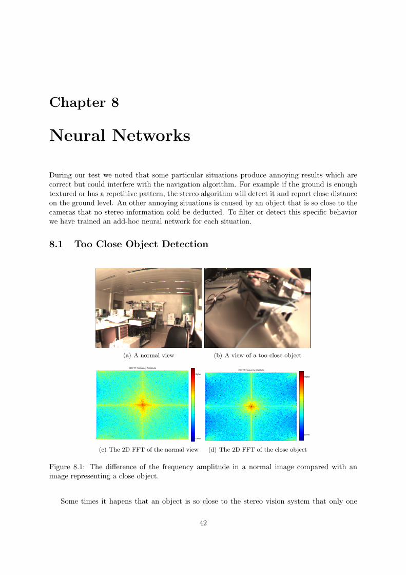
Chapter 8

Neural Networks

During our test we noted that some particular situations produce annoying results which arecorrect but could interfere with the navigation algorithm. For example if the ground is enoughtextured or has a repetitive pattern, the stereo algorithm will detect it and report close distanceon the ground level. An other annoying situations is caused by an object that is so close to thecameras that no stereo information cold be deducted. To filter or detect this specific behaviorwe have trained an add-hoc neural network for each situation.

8.1 Too Close Object Detection

(a) A normal view (b) A view of a too close object

2D FFT Frequency Amplitude

Lower

Higher

(c) The 2D FFT of the normal view

2D FFT Frequency Amplitude

Lower

Higher

(d) The 2D FFT of the close object

Figure 8.1: The difference of the frequency amplitude in a normal image compared with animage representing a close object.

Some times it hapens that an object is so close to the stereo vision system that only one

42

camera can see it. In such a situations the returned depth values are totally arbitrary, we wantto detect such a behavior and inform the obstacle avoidance algorithm. A common character-istic of too close objects is that they will result blurred since they are out of focus. Also theirtextures will result more homogeneous since we are looking at a small detail of a close object.This two characteristics leads us to believe that an image representing a close object shouldhave less important frequency than a normal one. To prouve or hipotesis we have operate a twodimensional FFT1 on two image samples, result are exposed in image 8.1. The neuronal net-work should easily find a space separation for the two category using the FFT as image feature.An other advantage is that the FFT is computationally optimized and will not deteriorate theglobal stereo computation frame rate.The neural architecture is composed by a single hidden layer and only allows forward connec-tions. There is 8193 input neurons equivalent to the FFT frequency domain of 128x128 pixelimage. As activation function we chose a hyperbolic tangent. The back-propagation method isused to train the neuronal network.

8.1.1 Training

0 10 20 30 40 500

0.05

0.1

0.15

0.2

0.25

0.3

0.35

0.4

0.45Training set Error

Mea

n Sq

uare

Erro

r Rat

e

Samples

(a) Training error

0 10 20 30 40 500.24

0.245

0.25

0.255

0.26

0.265

0.27

0.275

0.28M

ean

Squa

re E

rror R

ate

Samples

Validation set Error

(b) Validation error

Figure 8.2: Training and Validation Mean Square Error Rate

The Neural networks implementations are based on the Torch library [27] which providesclasses to model, and operate with the networks. To train our neural networks we have conceivedan application which grab a video flow and ask the user to categorize each frame. Frames canbe skipped or assigned to category A or B. For categorized frames the FFT is computed andstored on a buffer. Once the user chose to end the acquisition phase the buffers are empty anddata are routed in to two large data-set files. A trainer application will later use this data-setsfiles to create and train a neural network (the trainer application was inspired by a source codeprovided us by Matteo De Giacomi)We prepared a training and a test set, 100 samples for the training set, 50 sample of eachcategory. The test data set was smaller and contains a total of 50 samples. We generatedmultiples networks varying the number of hidden neurons from a minimum of 25 neurons to3500. The optimal solution for our data set is located around 100, figure 8.2 illustrate itstraining and validation function. The method to establish the most adapted number of hidden

1Fast Fourier Transform

43

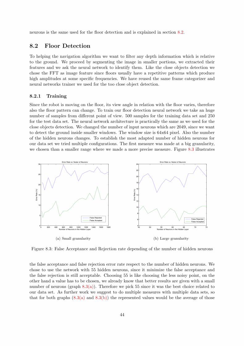
neurons is the same used for the floor detection and is explained in section 8.2.

8.2 Floor Detection

To helping the navigation algorithm we want to filter any depth information which is relativeto the ground. We proceed by segmenting the image in smaller portions, we extracted theirfeatures and we ask the neural network to identify them. Like the close objects detection wechose the FFT as image feature since floors usually have a repetitive patterns which producehigh amplitudes at some specific frequencies. We have reused the same frame categorizer andneural networks trainer we used for the too close object detection.

8.2.1 Training

Since the robot is moving on the floor, its view angle in relation with the floor varies, thereforealso the floor pattern can change. To train our floor detection neural network we take an hugenumber of samples from different point of view. 500 samples for the training data set and 250for the test data set. The neural network architecture is practically the same as we used for theclose objects detection. We changed the number of input neurons which are 2049, since we wantto detect the ground inside smaller windows. The window size is 64x64 pixel. Also the numberof the hidden neurons changes. To establish the most adapted number of hidden neurons forour data set we tried multiple configurations. The first measure was made at a big granularity,we chosen than a smaller range where we made a more precise measure. Figure 8.3 illustrates

0 200 400 600 800 1000 1200 1400 1600 18000

5

10

15

20

25

30

Number of Neurons in the Hidden Layer

Erro

r Rat

e (%

)

Error Rate vs. Nuber of Neurons

False RejectedFalse Accepted

(a) Small granularity

45 50 55 60 65 70 754

6

8

10

12

14

16

18

20

22

24Error Rate vs. Nuber of Neurons

Number of Neurons in the Hidden Layer

Erro

r Rat

e (%

)

False RejectedFalse Accepted

(b) Large granularity

Figure 8.3: False Acceptance and Rejection rate depending of the number of hidden neurons

the false acceptance and false rejection error rate respect to the number of hidden neurons. Wechose to use the network with 55 hidden neurons, since it minimize the false acceptance andthe false rejection is still acceptable. Choosing 55 is like choosing the less noisy point, on theother hand a value has to be chosen, we already know that better results are given with a smallnumber of neurons (graph 8.3(a)). Therefore we pick 55 since it was the best choice related toour data set. As further work we suggest to do multiple measures with multiple data sets, sothat for both graphs (8.3(a) and 8.3(b)) the represented values would be the average of those

44

measures and as consequence the local noise (error rate for a specific number of neurons) willbe reduced.

8.2.2 Application

We used the obtained neuronal networks to pre-filter the images before computing the depthmap. Unfortunately on a real application by testing the filters with the robot we discoveredthat obtained results are less reliable as expected. This is probably caused by some unexpectedinterferences, like the motion blur or other hazards. We could not further test the networks andtrain it with a larger data set to improve their performance.

45

Chapter 9

Conclusion

We have proposed a new robust correspondence algorithm especially conceived for vision guidedapplications. We have further analyzed its output and identified two inconvenient situations,which we want to avoid, in order to simplify the obstacle avoidance algorithm tasks. To overcomethis annoying behavior we propose a solution based on a neural network.The new correspondence algorithm has a preprocessing phase which, thanks to a combinationof two Difference-of-Gaussian functions, allows to filter un-textured image regions. We haveshown how the filter increases the quality of the disparity map, by filtering that correspondencewindows, which will probably yield to a miss match.We shown how an one-dimensional vertical smoothing can help to minimize the effects of abad image rectification. We found an alternative validity test to identify bad matches and wedemonstrated that it is less selective than the symmetric consistency check. A less selectivevalidity test is more adapted when handling close objects.In order to provide good quality images to our stereo algorithm we created the SynchronizedFrames Grabber, a driver, which allows to grab from a binocular firewire cameras system twoperfectly synchronized frames. We shown how a standalone external trigger is not enough toguarantee the synchronization and we proposed a reliable solution.We built together with Matteo De Giacomi an arena where we were able to test our solutions.We have compared our algorithm with the well know, and affirmed Small Vision System APIdeveloped by the SRI research institute and actually propriety of the Videre Design company.We are proud of our results since the project produced a stereo vision system, which has nothingto envy to his elder brother (the SVS of Videre Design).Finally we have proposed a solution to detect strange situations such as too close objects, whichare not detectable by the stereo engine. Also the floor can be detected and omitted from thedepth map, since it could cause confusion. Both filters are based on neural networks, we showedthat the FFT1 is good image feature to distinguish this cases. As further work we propose toprovide a bigger training data set, and make more massive tests to verify its usability for realapplications.

1Fast Fourier Transform

46

Bibliography

[1] A. Crespi and A.J. Ijspeert. AmphiBot II: An amphibious snake robot that crawls andswims using a central pattern generator. In Proceedings of the 9th International Conferenceon Climbing and Walking Robots (CLAWAR 2006), pages 19–27, 2006.

[2] A.J. Ijspeert and A. Crespi. Online trajectory generation in an amphibious snake robotusing a lamprey-like central pattern generator model. In Proceedings of the 2007 IEEEInternational Conference on Robotics and Automation (ICRA 2007), pages 262–268, 2007.

[3] A. Ijspeert, A. Crespi, D. Ryczko, and J.M. Cabelguen. From swimming to walking witha salamander robot driven by a spinal cord model. Science, 315(5817):1416–1420, 2007.

[4] O. Wulf and B. A. Wagner. Fast 3d scanning methods for laser measurement systems. July2003.

[5] Matteo De Giacomi. Robotics Applications of Vision-Based Action Selection. Master’sthesis, EPFL, August 2007. Very Frendly.

[6] V. Venkateswar and R. Chellappa. Hierarchical stereo and motion correspondence usingfeature groupings. Int. J. Comput. Vision, 15(3):245–269, 1995.

[7] Cordelia Schmid and Andrew Zisserman. The geometry and matching of curves in multipleviews. In ECCV (1), pages 394–409, 1998.

[8] U.R. Dhond and J.K. Aggarwal. Structure from stereo-a review. Systems, Man and Cy-bernetics, IEEE, 19:Page(s): 1489–1510, 1989.

[9] Daniel Scharstein and Richard Szeliski. A taxonomy and evaluation of dense two-framestereo correspondence algorithms. Int. J. Comput. Vision, 47(1-3):7–42, 2002.

[10] Myron Z. Brown, Darius Burschka, and Gregory D. Hager. Advances in computationalstereo. IEEE Trans. Pattern Anal. Mach. Intell., 25(8):993–1008, 2003.

[11] Andrew Dankers, Nick Barne, and Alexander Zelinsky. Active vision – rectification anddepth mapping. in Australian Conference on Robotics and Automation, 2004.

[12] C. Loop and Z. Zhang. Computing rectifying homographies for stereo vision. In TechnicalReport MSR-TR-99-21, 1999.

[13] Jean-Yves Bouguet. Camera calibration toolbox for matlab(http://www.vision.caltech.edu/bouguetj/calib doc/), 2007.

[14] Zhengyou Zhang. Determining the epipolar geometry and its uncertainty: A review. Int.J. Comput. Vision, 27(2):161–195, 1998.

47

[15] Zhengyou Zhang. A flexible new technique for camera calibration. IEEE Trans. PatternAnal. Mach. Intell., 22(11):1330–1334, 2000.

[16] Changming Sun. Fast stereo matching using rectangular subregioning and 3d maximum-surface techniques. Int. J. Comput. Vision, 47(1-3):99–117, 2002.

[17] Olivier Faugeras, B. Hotz, Herve Mathieu, T. Vieville, Zhengyou Zhang, Pascal Fua, EricTheron, Laurent Moll, Gerard Berry, Jean Vuillemin, Patrice Bertin, and Catherine Proy.Real time correlation based stereo: algorithm implementations and applications. TechnicalReport RR-2013, INRIA, 1993.

[18] D. W. Rosselot and E. L. Hall. Processing real-time stereo video for an autonomous robotusing disparity maps and sensor fusion. In D. P. Casasent, E. L. Hall, and J. Roning,editors, Intelligent Robots and Computer Vision XXII: Algorithms, Techniques, and ActiveVision. Edited by Casasent, David P.; Hall, Ernest L.; Roning, Juha. Proceedings of theSPIE, Volume 5608, pp. 70-78 (2004)., pages 70–78, October 2004.

[19] Heiko Hirschmuller, Peter R. Innocent, and Jon Garibaldi. Real-time correlation-basedstereo vision with reduced border errors. Int. J. Comput. Vision, 47(1-3):229–246, 2002.

[20] Luigi Di Stefano and Stefano Mattoccia. Real-time stereo within the videt project. Real-Time Imaging, 8(5):439–453, 2002.

[21] Heiko Hirschmuller. Improvements in real-time correlation-based stereo vision, 2001.

[22] H.K. Nishihara and T. Poggio. Stereo vision for robotics. First Int’l Symp. RoboticsResearch, pages 489–505, 1984.

[23] Pascal Fua. A parallel stereo algorithm that produces dense depth maps and preservesimage features. Springer Berlin / Heidelberg, 1993.

[24] Videre Design. Small vision system by videre design (http://www.videredesign.com/vision

[25] Pascal Fua. Combining stereo and monocular information to compute dense depth mapsthat preserve depth discontinuities. pages 1292–1298, 1991.

[26] David G. Lowe. Distinctive image features from scale-invariant keypoints. 60(2):91–110,November 2004.

[27] Ronan Collobert, Samy Bengio, and Johnny Mariethoz. Torche (http://www.torch.ch/).

48

Appendix A

Dynamic Programming Case Study

Table A.1: Normal Situations

Single object

Infinite distance

Tilt

49

Table A.2: Special Situations

Small escape

Dark

Too far

Too far 2

50

Appendix B

Distance at Disparity measure

Table B.1: Distance for Disparity measure

cm disp130 11120 12110 13100 1490 1680 1770 1960 2250 2740 3230 3820 6016 81

51

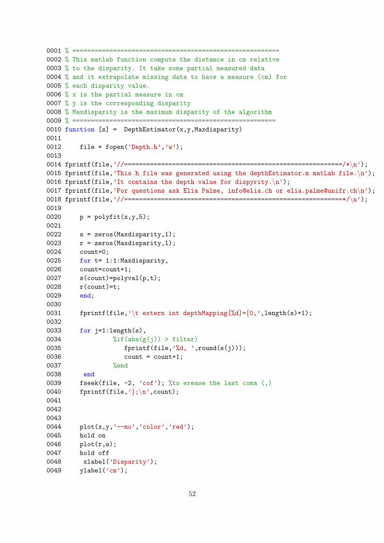
0001 % ========================================================0002 % This matlab function compute the distance in cm relative0003 % to the disparity. It take some partial measured data0004 % and it extrapolate missing data to have a measure (cm) for0005 % each disparity value.0006 % x is the partial measure in cm0007 % y is the corresponding disparity0008 % Maxdisparity is the maximum disparity of the algorithm0009 % =======================================================0010 function [s] = DepthEstimator(x,y,Maxdisparity)00110012 file = fopen(’Depth.h’,’w’);00130014 fprintf(file,’//===========================================================/*\n’);0015 fprintf(file,’This h file was generated using the depthEstimator.m matLab file.\n’);0016 fprintf(file,’It contains the depth value for dispyrity.\n’);0017 fprintf(file,’For questions ask Elia Palme, [email protected] or [email protected]\n’);0018 fprintf(file,’//===========================================================*/\n’);00190020 p = polyfit(x,y,5);00210022 s = zeros(Maxdisparity,1);0023 r = zeros(Maxdisparity,1);0024 count=0;0025 for t= 1:1:Maxdisparity,0026 count=count+1;0027 s(count)=polyval(p,t);0028 r(count)=t;0029 end;00300031 fprintf(file,’\t extern int depthMapping[%d]={0,’,length(s)+1);00320033 for j=1:length(s),0034 %if(abs(g(j)) > filter)0035 fprintf(file,’%d, ’,round(s(j)));0036 count = count+1;0037 %end0038 end0039 fseek(file, -2, ’cof’); %to erease the last coma (,)0040 fprintf(file,’};\n’,count);0041004200430044 plot(x,y,’--mo’,’color’,’red’);0045 hold on0046 plot(r,s);0047 hold off0048 xlabel(’Disparity’);0049 ylabel(’cm’);

52

0050 title(’Distance at Disparity’);0051 legend(’Measured data’,’Extrapolate data’);00520053 fclose(file);

53

Appendix C

MatLab code to test thedifference-of-Gausian filter

54

0001 %==========================================================================0002 %ex values: computeWindowsTest(’test.png’,96,0.4,3.35,24)0003 %==========================================================================0004 function [f] = computeWindowsTest(filename,l,initSigma1,scale,kernleSize)0005 input = extractLine(filename,l);0006 line = cast(input, ’single’);0007 %trashold = 0.0004;0008 [h,w,d]=size(line);0009 X = 0:1:w-1;0010 numScale=2;0011 r = zeros(numScale,w);0012 p = zeros(1,w);0013 x = kernleSize/2*-1:1:kernleSize/2-1+1;001400150016 %==========================================================================0017 %Using the DOG operator (Difference of gausian) convolute tha image row00180019 g1 = DOG (x,initSigma1,initSigma1+scale);0020 g2 = DOG (x,initSigma1+scale,initSigma1+2*scale);002100220023 %Apply the convolution using the computed DOG function0024 for m=kernleSize/2:w-(kernleSize/2)-1+1,0025 filter = zeros(1,kernleSize);00260027 for d=-(kernleSize/2):(kernleSize/2)-1,0028 % if(abs(g(j)) > trashold)0029 filter(d+(kernleSize/2)+1) =(line(m+d+1) * g1(d+(kernleSize/2)+1));0030 %end0031 end0032 r(1,m)=abs(sum(filter));0033 end00340035 for m=kernleSize/2:w-(kernleSize/2)-1+1,0036 filter = zeros(1,kernleSize);00370038 for d=-(kernleSize/2):(kernleSize/2)-1,0039 % if(abs(g(j)) > trashold)0040 filter(d+(kernleSize/2)+1) =(line(m+d+1) * g2(d+(kernleSize/2)+1));0041 %end0042 end0043 r(2,m)=abs(sum(filter));0044 end004500460047 %==========================================================================0048 %The windows scale correspond to the scale which hase the maxim difference0049 for m=kernleSize/2:w-(kernleSize/2)-1,

55

00500051 max=-1;0052 maxIndex=1;0053 for j=1:numScale,00540055 if(r(j,m) > max)0056 max= r(j,m);0057 maxIndex=j;0058 end0059 end0060 p(m)= maxIndex;0061 end006200630064 figure(’Name’, ’Result’);0065 grapf = subplot(2,1,1);plot(X,line);0066 axis(grapf,[0 w 0 260]);0067 xlabel(’x (coordonate)’);0068 ylabel(’y (pixel intensity)’);0069 title(’One pixels raw of an image in gray scale’);0070 %legend(’pixel intensity’);0071 grapf = subplot(2,1,2);plot(X,p);0072 axis(grapf,[0 w 0 numScale + (0.5*numScale)]);0073 xlabel(’x (coordonate)’);0074 ylabel(’scale’);0075 title(’Difference of Gaussian scale having the highest value’);0076 legend([’Initial sigma: ’,

num2str(initSigma1),’, scale factor: ’,num2str(scale),’, kernel size ’,num2str(kernleSize),’px’]);

00770078 %==========================================================================0079 %DOG operator compute the difference of gausian function0080 function [g] = DOG (x,o1,o2)0081 y = 1/sqrt(2*pi) * ( 1 / o1 * exp(-(x.^2)/(2*o1^2)) - 1 / o2 *

exp(-(x.^2)/(2*o2^2)));0082 g = cast(y, ’single’);00830084 function [p] = extractLine(filename,l)0085 I = imread(filename);0086 [h,w,d]=size(I);0087 p = I(l:l,1:w);00880089 function [g] = gaussian(x,o)0090 g = (1/sqrt(2*pi*o^2) ) * exp ( - x.^2 / (2 * o^2));

56

Appendix D

MatLab code to generate the .h filecontaining the difference-of-Gaussianfilter constants

57

0001 %==========================================================================0002 %Find the size of the correlation window for each pixel postion of an image0003 %row. Depending on the pixels intensity omogeneity arround that pixel0004 %position.0005 %PARAMETERS:0006 %filename : the png file containing the image0007 %l: the image row to analize.0008 %scaleFactor: how mach increase the scale at ecah iteration (usualy 1)0009 %numScale: how many scales0010 %ex values: computeWindows(0.6,1.55,1,2,12)0011 %better values: computeWindows(2,1.4,1.2,2,24),0012 %computeWindows(1.7,1.8,1.2,2,24)0013 %==========================================================================0014 function [f] = computeScaleDOG(initSigma1, scale ,kernleSize)00150016 x = kernleSize/2*-1:1:kernleSize/2-1+1;0017 x2 = kernleSize/2*-1:0.1:kernleSize/2-1+1;00180019 file = fopen(’DOGfilter.h’,’w’);00200021 fprintf(file,’//============================================================/*\n’);0022 fprintf(file,’This h file was generated using the computeWindows.m matLab file.\n’);0023 fprintf(file,’It contains multiple DOG function in different scales.\n’);0024 fprintf(file,’For questions ask Elia Palme, [email protected] or [email protected]\n’);0025 fprintf(file,’//===========================================================*/\n’);00260027 fprintf(file,’struct dogFilter{\n’);0028 fprintf(file,’\tfloat values[%d];\n’,kernleSize+1);0029 fprintf(file,’\tint kernelSize;\n’);0030 fprintf(file,’};\n’);00310032 fprintf(file,’struct dogScales{\n’);0033 fprintf(file,’\tint numScales;\n’);0034 fprintf(file,’\tint maxKernelSize;\n’);0035 fprintf(file,’\tdogFilter scales[%d];\n’,2);0036 fprintf(file,’};\n’);003700380039 %==========================================================================0040 %Using the DOG operator (Difference of gausian) convolute tha image row0041 figure(’Name’, ’DOG’);00420043 g1 = DOG (x,initSigma1,initSigma1+scale);0044 g2 = DOG (x,initSigma1+scale,initSigma1+2*scale);00450046 g1t = DOG (x2,initSigma1,initSigma1+scale);0047 g2t = DOG (x2,initSigma1+scale,initSigma1+2*scale);00480049 tempg1 = gaussian(x2,initSigma1);

58

0050 tempg2 = gaussian(x2,initSigma1+scale);0051 tempg3 = gaussian(x2,initSigma1+2*scale);00520053 printToFile(g1,1,file);0054 printToFile(g2,2,file);00550056 plot(x2, tempg1, ’-’, x2, tempg2, ’--’,x2,tempg3,’-.’,

’LineWidth’,1,’MarkerSize’,2),axis([-8 8 0 .3]), grid on;0057 legend([’\sigma = ’,num2str(initSigma1)],

[’\sigma = ’,num2str(initSigma1+scale)],[’\sigma = ’,num2str(initSigma1+2*scale)])

0058 xlabel(’x’), ylabel(’Density Probabilities’),0059 title(’Gaussians’)006000610062 figure(2);0063 plot(x2, g1t,’-’,x2,g2t,’--’),axis([-8 8 -0.15 .20]), grid on;0064 xlabel(’x’), ylabel(’y’),0065 title(’Difference of Gaussian’);006600670068 f=0;00690070 fprintf(file,’dogScales dog = { %d,%d,{’,2,kernleSize+1);007100720073 fprintf(file,’f%d, ’,1);0074 fprintf(file,’f%d, ’,2);00750076 fseek(file, -2, ’cof’); %to erease the last coma (,)0077 fprintf(file,’} };\n’);007800790080 fclose(file);0081008200830084 %==========================================================================0085 %save the DOG function0086 function [x] = printToFile(g,s,file)00870088 count =0;0089 fprintf(file,’dogFilter f%d={{’,s);00900091 for j=1:size(g,2),0092 %if(abs(g(j)) > filter)0093 fprintf(file,’%ff, ’,g(j));0094 count = count+1;0095 %end

59

0096 end0097 fseek(file, -2, ’cof’); %to erease the last coma (,)0098 fprintf(file,’},%d};\n’,count);009901000101 %==========================================================================0102 %DOG operator compute the difference of gausian function0103 function [g] = DOG (x,o1,o2)0104 y = 1/sqrt(2*pi) * ( 1 / o1 * exp(-(x.^2)/(2*o1^2)) - 1 / o2 *

exp(-(x.^2)/(2*o2^2)));0105 g = cast(y, ’single’);01060107 function [p] = extractLine(filename,l)0108 I = imread(filename);0109 [h,w,d]=size(I);0110 p = I(l:l,1:w);01110112 function [g] = gaussian(x,o)0113 g = (1/sqrt(2*pi*o^2) ) * exp ( - x.^2 / (2 * o^2));

60

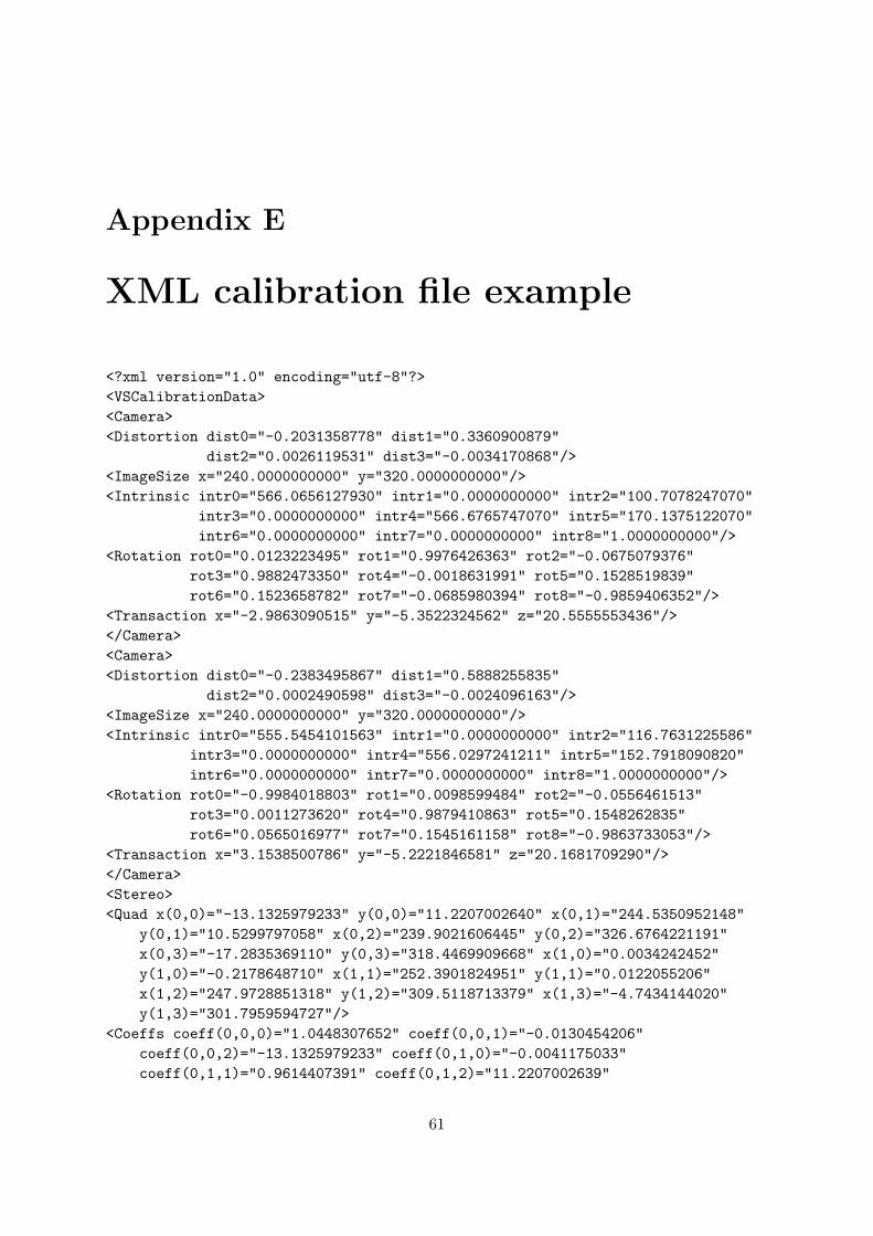
Appendix E

XML calibration file example

<?xml version="1.0" encoding="utf-8"?><VSCalibrationData><Camera><Distortion dist0="-0.2031358778" dist1="0.3360900879"

dist2="0.0026119531" dist3="-0.0034170868"/><ImageSize x="240.0000000000" y="320.0000000000"/><Intrinsic intr0="566.0656127930" intr1="0.0000000000" intr2="100.7078247070"

intr3="0.0000000000" intr4="566.6765747070" intr5="170.1375122070"intr6="0.0000000000" intr7="0.0000000000" intr8="1.0000000000"/>

<Rotation rot0="0.0123223495" rot1="0.9976426363" rot2="-0.0675079376"rot3="0.9882473350" rot4="-0.0018631991" rot5="0.1528519839"rot6="0.1523658782" rot7="-0.0685980394" rot8="-0.9859406352"/>

<Transaction x="-2.9863090515" y="-5.3522324562" z="20.5555553436"/></Camera><Camera><Distortion dist0="-0.2383495867" dist1="0.5888255835"

dist2="0.0002490598" dist3="-0.0024096163"/><ImageSize x="240.0000000000" y="320.0000000000"/><Intrinsic intr0="555.5454101563" intr1="0.0000000000" intr2="116.7631225586"

intr3="0.0000000000" intr4="556.0297241211" intr5="152.7918090820"intr6="0.0000000000" intr7="0.0000000000" intr8="1.0000000000"/>

<Rotation rot0="-0.9984018803" rot1="0.0098599484" rot2="-0.0556461513"rot3="0.0011273620" rot4="0.9879410863" rot5="0.1548262835"rot6="0.0565016977" rot7="0.1545161158" rot8="-0.9863733053"/>

<Transaction x="3.1538500786" y="-5.2221846581" z="20.1681709290"/></Camera><Stereo><Quad x(0,0)="-13.1325979233" y(0,0)="11.2207002640" x(0,1)="244.5350952148"

y(0,1)="10.5299797058" x(0,2)="239.9021606445" y(0,2)="326.6764221191"x(0,3)="-17.2835369110" y(0,3)="318.4469909668" x(1,0)="0.0034242452"y(1,0)="-0.2178648710" x(1,1)="252.3901824951" y(1,1)="0.0122055206"x(1,2)="247.9728851318" y(1,2)="309.5118713379" x(1,3)="-4.7434144020"y(1,3)="301.7959594727"/>

<Coeffs coeff(0,0,0)="1.0448307652" coeff(0,0,1)="-0.0130454206"coeff(0,0,2)="-13.1325979233" coeff(0,1,0)="-0.0041175033"coeff(0,1,1)="0.9614407391" coeff(0,1,2)="11.2207002639"

61

coeff(0,2,0)="-0.0001177116" coeff(0,2,1)="0.0000042663"coeff(0,2,2)="1.0000000000" coeff(1,0,0)="1.0262211635"coeff(1,0,1)="-0.0148082858" coeff(1,0,2)="0.0034242452"coeff(1,1,0)="0.0009573988" coeff(1,1,1)="0.9421653755"coeff(1,1,2)="-0.2178648710" coeff(1,2,0)="-0.0001005995"coeff(1,2,1)="-0.0000053938" coeff(1,2,2)="1.0000000000"/>

</Stereo></VSCalibrationData>

62

Appendix F

Trigger micro controller C code

#include "triggerController.h"

volatile int1 b;#int_RDA

//============================// Interruption routine//============================void RDA_isr(void) {char c;c = getc(); //empty the UART buffer//printf("\x1b[1m%d\x1b[m ", c); //DEBUGb = !b;}

void main(){

setup_adc_ports(NO_ANALOGS|VSS_VDD);setup_adc(ADC_OFF|ADC_TAD_MUL_0);setup_spi(SPI_SS_DISABLED);setup_wdt(WDT_OFF);setup_timer_0(RTCC_INTERNAL);setup_timer_1(T1_DISABLED);setup_timer_2(T2_DISABLED,0,1);setup_timer_3(T3_DISABLED|T3_DIV_BY_1);setup_vref(FALSE);enable_interrupts(INT_RDA);enable_interrupts(GLOBAL);

output_high(PIN_B0); //Cameras work with inverted 1/0

//============================// Main loop

63

//============================

while (1) {

if (b) {output_high(PIN_C2); //Basler camerasoutput_high(PIN_A0); //ledoutput_low(PIN_B0); //Point Grey camerasdelay_ms(20);output_low(PIN_C2);output_low(PIN_A0);output_high(PIN_B0);b = !b;}

}}

64

Appendix G

BibTeX reference

@mastersthesis{EPalmeTechRep,Author = {Elia Palme},Date-Added = {2007-07-18 11:54:42 +0200},Date-Modified = {2007-08-18 12:33:18 +0200},Institution = {UNIFR and EPFL},Keywords = {Stereo Vision System, Correspondence Algorithm, Robotics,Obstacle Avoidance Applications, Real Time, Trigger, Synchronized Frames Grabber,SSD Correlation, Difference of Gaussians, Neural Network},Month = {8},School = {University of Fribourg and EPFL, Switzerland},Title = {Stero Vison Library for Obstacle Advoidance Applications},Type = {Master Project Tecnical Report},Url = {http://www.elia.ch},Year = {2008}}

65

stereo vision library for obstacle avoidance applications

Documents