STELLAR SPECTRA

B. LTE Line Formation

R.J. Rutten

Sterrekundig Instituut Utrecht

May 9, 2003

Copyright c© 1999 Robert J. Rutten, Sterrekundig Instuut Utrecht, The Netherlands.Copying permitted exclusively for non-commercial educational purposes, courtesy of the Euro-pean Solar Magnetometry Network (http://www.astro.uu.nl/∼rutten/tmr).

Contents

Introduction 1

1 Stratification of the solar atmosphere 3

1.1 FALC temperature stratification . . . . . . . . . . . . . . . . . . . . . . . . . . . 41.2 FALC density stratification . . . . . . . . . . . . . . . . . . . . . . . . . . . . . . 51.3 Comparison with the earth’s atmosphere . . . . . . . . . . . . . . . . . . . . . . . 61.4 Discussion . . . . . . . . . . . . . . . . . . . . . . . . . . . . . . . . . . . . . . . . 7

2 Continuous spectrum from the solar atmosphere 11

2.1 Observed solar continua . . . . . . . . . . . . . . . . . . . . . . . . . . . . . . . . 112.2 Continuous extinction . . . . . . . . . . . . . . . . . . . . . . . . . . . . . . . . . 132.3 Optical depth . . . . . . . . . . . . . . . . . . . . . . . . . . . . . . . . . . . . . . 142.4 Emergent intensity and height of formation . . . . . . . . . . . . . . . . . . . . . 152.5 Disk-center intensity . . . . . . . . . . . . . . . . . . . . . . . . . . . . . . . . . . 162.6 Limb darkening . . . . . . . . . . . . . . . . . . . . . . . . . . . . . . . . . . . . . 162.7 Flux integration . . . . . . . . . . . . . . . . . . . . . . . . . . . . . . . . . . . . 172.8 Discussion . . . . . . . . . . . . . . . . . . . . . . . . . . . . . . . . . . . . . . . . 18

3 Spectral lines from the solar atmosphere 21

3.1 Observed Na D line profiles . . . . . . . . . . . . . . . . . . . . . . . . . . . . . . 213.2 Na D wavelengths . . . . . . . . . . . . . . . . . . . . . . . . . . . . . . . . . . . . 213.3 LTE line formation . . . . . . . . . . . . . . . . . . . . . . . . . . . . . . . . . . . 233.4 Line extinction . . . . . . . . . . . . . . . . . . . . . . . . . . . . . . . . . . . . . 233.5 Line broadening . . . . . . . . . . . . . . . . . . . . . . . . . . . . . . . . . . . . . 243.6 Implementation . . . . . . . . . . . . . . . . . . . . . . . . . . . . . . . . . . . . . 253.7 Computed Na D1 line profile . . . . . . . . . . . . . . . . . . . . . . . . . . . . . . 253.8 Discussion . . . . . . . . . . . . . . . . . . . . . . . . . . . . . . . . . . . . . . . . 25

References 27

These exercises are available at http://www.astro.uu.nl/∼rutten/ssb.

Introduction

These three exercises treat the formation of spectral lines in the solar atmosphere assumingLocal Thermodynamical Equilibrium (LTE). The topics are:

• stratification of the solar atmosphere;

• formation of the continuous solar spectrum;

• formation of Fraunhofer lines in the solar spectrum.

The method consists of experimentation using IDL. The exercises require knowledge of basicradiative transfer.

These exercises are a sequel to the exercises “Stellar Spectra A: Basic Line Formation”. Thetwo sets are independent in the sense that you don’t have to have worked through the firstset to do the present set. However, various concepts needed in the present set are treated inthe second and third exercises of the first set and some of the programs constructed there areuseful here, so that it may be of interest to you to go through these quickly. They are found athttp://www.astro.uu.nl/∼rutten/ssa/ as files:

– ssa.ps.gz = gzipped PostScript instruction (including an IDL manual);

– ssa2.idl = IDL code 2nd exercise (Saha-Boltzmann modeling);

– ssa3.idl = IDL code 3rd exercise (Schuster-Schwarzschild modeling).

Your report on these exercises should include pertinent graphs made with IDL. A LaTeXtemplate that you may adopt for writing a report is available as file ssreport.tpl athttp://www.astro.uu.nl/∼rutten/rrtex/templates/. A brief LaTeX style manual is foundin ss_manual.txt at http://www.astro.uu.nl/∼rutten/rrtex/manuals/students/.

1

Table 1: Selected units and constants. Precise values available at http://physics.nist.gov/cuu/Constants.

1 A = 0.1 nm = 10−8 cm

1 erg = 10−7 Joule

1 dyne cm−2 = 0.1 Pascal = 10−6 bar = 9.8693 × 10−7 atmosphere

energy of 1 eV= 1.60219 × 10−12 erg

photon energy (in eV) E = 12398.55/λ (in A)

speed of light c = 2.99792 × 1010 cm s−1

Planck constant h = 6.62607 × 10−27 erg s

Boltzmann constant k = 1.38065 × 10−16 erg K−1

= 8.61734 × 10−5 eVK−1

electron mass me = 9.10939 × 10−28 g

proton mass mp = 1.67262 × 10−24 g

atomic mass unit (amu, C=12) mA = 1.66054 × 10−24 g

first Bohr orbit radius a0 = 0.529178 × 10−9 cm

hydrogen ionization energy χH = 13.598 eV

solar mass M = 1.9891 × 1033 g

solar radius R = 6.9599 × 1010 cm

distance sun – earth AE = 1.49598 × 1013 cm

earth mass M⊕ = 5.976 × 1027 g

earth radius R⊕ = 6.3710 × 108 cm

2

1 Stratification of the solar atmosphere

In this exercise you study the radial stratification of the solar atmosphere on the basis of thestandard model FALC by Fontenla et al. (1993). They derived this description of the solarphotosphere and chromosphere empirically, assuming that the solar atmosphere is horizontallyhomogeneous (“plane parallel layers”) and in hydrostatic equilibrium (“time independent”).

Figure 1: Eugene H. Avrett (born 1933) represents the A in the VAL (Vernazza, Avrett and Loeser)and FAL (Fontenla, Avrett and Loeser) sequences of standard models of the solar atmosphere. At theCenter for Astrophysics (Cambridge, Mass.) he developed, together with programmer Rudolf Loeser, anenormous spectrum modeling code (called Pandora, perhaps a fitting name) which fits observed solarcontinua and lines throughout the spectrum through the combination of trial-and-error adjustment ofthe temperature stratification with simultaneous evaluation of the corresponding particle densities withgreat sophistication, basically performing complete NLTE population analysis for all key transitions inthe solar spectrum. His VALIII paper (Vernazza, Avrett and Loeser 1981) stands as one of the threeprime solar physics papers of the second half of the twentieth century (with Parker’s 1958 solar windprediction and Ulrich’s 1970 p-mode prediction). Photograph copied from Strassmeier and Linsky (1996).

The FALC model is specified in Tables 3–4 and in file falc.dat1. Copy this file to your workdirectory.

The first column in Tables 3–4 specifies the height h which is the distance above τ500 = 1 whereτ500, given in the second column, is the radial optical depth in the continuum at λ = 500 nm.The quantity m in the third column is the mass of a column with cross-section 1 cm2 above thegiven location.

In the photosphere (−100 ≤ h ≤ 525 km) and chromosphere (525 ≤ h ≤ 2100 km) the tem-perature T (fourth column) has been adjusted empirically so that the computed spectrum isin agreement with the spatially averaged disk-center spectrum observed from quiet solar ar-eas (away from active regions). The temperature distribution in the transition region (aboveh ≈ 2100 km, up to T = 105 K) has been determined theoretically by balancing the downflow ofenergy from the corona through thermal conduction and diffusion against the radiative energylosses.

The microturbulent velocity vt roughly accounts for the Doppler broadening that is observed toexceed the thermal broadening of lines formed at various heights. The total pressure Ptot is the

1With other IDL input files available at http://www.astro.uu.nl/∼rutten/ssb/.

3

Figure 2: Temperature stratification of the FALC model. The height scale has h = 0 at the location withτ500 = 1. The photosphere reaches until h = 525 km (temperature minimum). The chromosphere higherup has a mild temperature rise out to h ≈ 2100 km where the steep increase to the 1–2 MK corona starts(”transition region”).

sum of the gas pressure Pgas and the corresponding turbulent pressure ρ v2t /2 where ρ is the gas

density (last column).

The tables also lists the total hydrogen density nH, the free proton density np, and the freeelectron density ne. Given the T and vt distributions with height, these number densitiesand other quantities were determined by requiring hydrostatic equilibrium and evaluating theionization balances by solving the coupled radiative transfer and statistical equilibrium equations(without assuming LTE). The adopted helium-to-hydrogen abundance ratio is NHe/NH = 0.1.The relative abundances of the other elements came from Anders and Grevesse (1989).

1.1 FALC temperature stratification

Figure 2 shows the FALC temperature stratification. It was made with IDL code similar to thefollowing (supplied in file readfalc.idl):

; file: readfalc.idl = IDL main to read & plot falc.dat = FALC model

; last: May 7 1999

; note: file FALC.DAT from email Han Uitenbroek Apr 29 1999

; = resampled Table 2 of Fontenla et al ApJ 406 319 1993

; = 2 LaTeX tables in file falc.tex

; read falc model

close,1

openr,1,’falc.dat’

nh=80 ; nr FALC height values

falc=fltarr(11,nh) ; 11 FALC columns

4

readf,1,falc ; this may be done more elegantly with IDL structure

h=falc(0,*) ; but I don’t know (yet) how

tau5=falc(1,*)

colm=falc(2,*)

temp=falc(3,*)

vturb=falc(4,*)

nhyd=falc(5,*)

nprot=falc(6,*)

nel=falc(7,*)

ptot=falc(8,*)

pgasptot=falc(9,*)

dens=falc(10,*)

; plot falc model

plot,h,temp,yrange=[3000,10000],$

xtitle=’height [km]’,ytitle=’temperature [K]’

; repeat plot on postscript file

set_plot,’ps’ ; repeat plot on PostScript file

device,filename=’falc_temp_height.ps’

plot,h,temp,yrange=[3000,10000],$

xtitle=’height [km]’,ytitle=’temperature [K]’

device,/close

set_plot,’x’ ; return to screen; set_plot,’win’ for Windows

end

• Pull this code over and make it work.

1.2 FALC density stratification

We will now study relations between various FALC model parameters. This is easiest done bytrying out plots on the IDL command line after running an IDL main program such as theone above. You will often need to generate logarithmic axes with keywords /xlog and /ylog

in command plot, and you will also need keyword \ynozero to plot y-axes without extensiondown to y = 0. Various constants are specified in Table 1 on page 2.

• Plot the total pressure ptotal against the column mass m, both linearly and logarithmically.You will find that they scale linearly. Explain what assumption has caused ptotal = cm anddetermine the value of the solar surface gravity gsurface = c that went into the FALC-producingcode.

• Fontenla et al. (1993) also assumed complete mixing, i.e., the same element mix at all heights.Check this by plotting the ratio of the hydrogen mass density to the total mass density againstheight (the hydrogen atom mass is mH = 1.67352 × 10−24 g, e.g., Allen 1976). Then addhelium to hydrogen using their abundance and mass ratios (NHe/NH = 0.1, mHe = 3.97mH),and estimate the fraction of the total mass density made up by the remaining elements inthe model mix (the “metals”).

• Plot the column mass against height. The curve becomes nearly straight when you make the

5

y-axis logarithmic. Why is that? Why isn’t it exactly straight?

• Plot the gas density against height. Estimate the density scale height Hρ in ρ ≈ρ(0) exp(−h/Hρ) in the deep photosphere.

• Compute the gas pressure and plot it against height. Overplot the product (nH+ne) kT . Plotthe ratio of the two curves to show their differences. Do the differences measure deviationsfrom the ideal gas law or something else? Now add the helium density NHe to the productand enlarge the deviations. Comments?

• Plot the hydrogen density against height and overplot curves for the electron and protondensities. Explain their behavior. You may find inspiration in Figure 6 on page 13.

• Plot the ionization fraction of hydrogen logarithmically against height. Why does this curvelook like the one in Figure 2? And why is it tilted with respect to that?

• Let us now compare the photon and particle densities. In thermodynamic equilibrium (TE)the radiation is isotropic with intensity Iν = Bν and has total energy density (Stefan Boltz-mann)

u =1

c

∫∫

Bν dΩ dν =4σ

cT 4, (1)

so that the total photon density for isotropic TE radiation is given, with uν = du/dν, T inK and Nphot in photons per cm3, by

Nphot =

∫

∞

0

uν

hνdν ≈ 20T 3. (2)

This equation gives a reasonable estimate for the photon density at the deepest model loca-tion, why? Compute the value there and compare it to the hydrogen density. Why is the equa-tion not valid higher up in the atmosphere? The photon density there is Nphot ≈ 20T 3

eff/2πwith Teff = 5770 K the effective solar temperature (since πB(Teff) = σT 3

eff = F+ = πI+

with F+ the emergent flux and I+ the disk-averaged emergent intensity). Compare it to thehydrogen density at the top of the FALC model. The medium there is insensitive to thesephotons (except those at the center wavelength of the hydrogen Lyα line), why?.

1.3 Comparison with the earth’s atmosphere

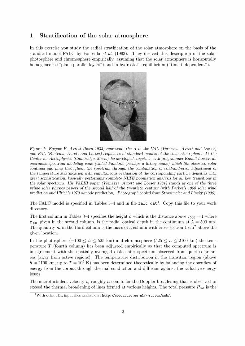
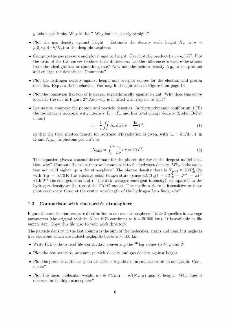
Figure 3 shows the temperature distribution in our own atmosphere. Table 2 specifies its averageparameters (the original table in Allen 1976 continues to h = 50 000 km). It is available as fileearth.dat. Copy this file also to your work directory.

The particle density in the last column is the sum of the molecules, atoms and ions, but neglectsfree electrons which are indeed negligible below h ≈ 100 km.

• Write IDL code to read file earth.dat, converting the 10 log values to P , ρ and N .

• Plot the temperature, pressure, particle density and gas density against height.

• Plot the pressure and density stratifications together in normalized units in one graph. Com-ments?

• Plot the mean molecular weight µE ≡ m/mH = ρ/(N mH) against height. Why does itdecrease in the high atmosphere?

6

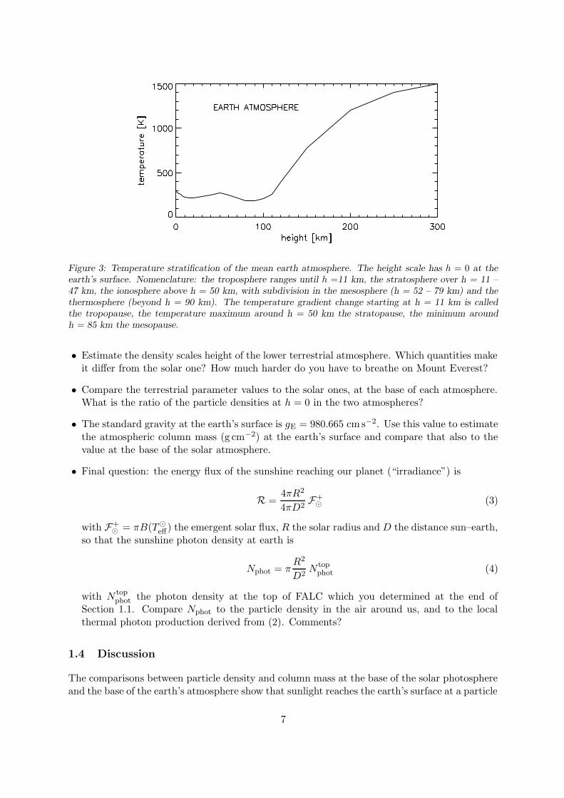
Figure 3: Temperature stratification of the mean earth atmosphere. The height scale has h = 0 at theearth’s surface. Nomenclature: the troposphere ranges until h =11 km, the stratosphere over h = 11 –47 km, the ionosphere above h = 50 km, with subdivision in the mesosphere (h = 52 – 79 km) and thethermosphere (beyond h = 90 km). The temperature gradient change starting at h = 11 km is calledthe tropopause, the temperature maximum around h = 50 km the stratopause, the minimum aroundh = 85 km the mesopause.

• Estimate the density scales height of the lower terrestrial atmosphere. Which quantities makeit differ from the solar one? How much harder do you have to breathe on Mount Everest?

• Compare the terrestrial parameter values to the solar ones, at the base of each atmosphere.What is the ratio of the particle densities at h = 0 in the two atmospheres?

• The standard gravity at the earth’s surface is gE = 980.665 cm s−2. Use this value to estimatethe atmospheric column mass (g cm−2) at the earth’s surface and compare that also to thevalue at the base of the solar atmosphere.

• Final question: the energy flux of the sunshine reaching our planet (“irradiance”) is

R =4πR2

4πD2F+ (3)

with F+ = πB(T

eff) the emergent solar flux, R the solar radius and D the distance sun–earth,so that the sunshine photon density at earth is

Nphot = πR2

D2N top

phot (4)

with N topphot the photon density at the top of FALC which you determined at the end of

Section 1.1. Compare Nphot to the particle density in the air around us, and to the localthermal photon production derived from (2). Comments?

1.4 Discussion

The comparisons between particle density and column mass at the base of the solar photosphereand the base of the earth’s atmosphere show that sunlight reaches the earth’s surface at a particle

7

density that is much higher than the density at the sunlight τ = 1 escape location within thesun, i.e., the atmospheric depth where the solar gas becomes opaque. If, reversely, the earthwere irradiating the sun, that level is where the earthshine would stop already, having passedthrough a much smaller amount of solar gas then it went through in the nearly transparantearth atmosphere (transmission 80% at λ = 500 nm at sea level when the sky is clear, Allen1976).

Thus, the solar gas is much more opaque per particle than air, even though the terrestrial airparticles (molecules) are much larger than the solar atmospheric particles (mostly hydrogenatoms and electrons). In the first decades of the twentieth century the source of this very largeopacity was an unsolved riddle as important as the quest for the subatomic energy source thatmakes the sun shine (for example, see the eloquent last paragraph of Eddington’s “The InternalConstitution of the Stars”). That opacity is the topic of the next exercise.

Table 2: Earth atmosphere, from Allen (1976).

h log P T log ρ log Nkm dyn cm−2 K g cm−3 cm−3

0 6.01 288 –2.91 19.41

1 5.95 282 –2.95 19.36

2 5.90 275 –3.00 19.31

3 5.85 269 –3.04 19.28

4 5.79 262 –3.09 19.23

5 5.73 256 –3.13 19.19

6 5.67 249 –3.18 19.14

8 5.55 236 –3.28 19.04

10 5.42 223 –3.38 18.98

15 5.08 217 –3.71 18.61

20 4.75 217 –4.05 18.27

30 4.08 230 –4.74 17.58

40 3.47 253 –5.39 16.92

50 2.91 273 –5.98 16.34

60 2.36 246 –6.50 15.82

70 1.73 216 –7.07 15.26

80 1.00 183 –7.72 14.60

90 0.19 183 –8.45 13.80

100 –0.53 210 –9.30 12.98

110 –1.14 260 –10.00 12.29

120 –1.57 390 –10.62 11.69

150 –2.32 780 –11.67 10.66

200 –3.06 1200 –12.50 9.86

250 –3.55 1400 –13.10 9.30

300 –4.00 1500 –13.60 8.90

8

Table 3: FALC model, part 1.

h τ500 m T vt nH np ne Ptot Pgas/Ptot ρkm g cm−2 K kms−1 cm−3 cm−3 cm−3 dyn cm−2 g cm−3

2218.20 0.00E+00 6.777E−06 100000 11.73 5.575E+09 5.575E+09 6.665E+09 1.857E−01 0.952 1.31E−14

2216.50 7.70E−10 6.779E−06 95600 11.65 5.838E+09 5.837E+09 6.947E+09 1.857E−01 0.950 1.37E−14

2214.89 1.53E−09 6.781E−06 90816 11.56 6.151E+09 6.150E+09 7.284E+09 1.858E−01 0.948 1.44E−14

2212.77 2.60E−09 6.785E−06 83891 11.42 6.668E+09 6.667E+09 7.834E+09 1.859E−01 0.945 1.56E−14

2210.64 3.75E−09 6.788E−06 75934 11.25 7.381E+09 7.378E+09 8.576E+09 1.860E−01 0.941 1.73E−14

2209.57 4.38E−09 6.790E−06 71336 11.14 7.864E+09 7.858E+09 9.076E+09 1.860E−01 0.938 1.84E−14

2208.48 5.06E−09 6.792E−06 66145 11.02 8.488E+09 8.476E+09 9.718E+09 1.861E−01 0.935 1.99E−14

2207.38 5.81E−09 6.794E−06 60170 10.86 9.334E+09 9.307E+09 1.059E+10 1.862E−01 0.931 2.19E−14

2206.27 6.64E−09 6.797E−06 53284 10.67 1.053E+10 1.047E+10 1.182E+10 1.862E−01 0.925 2.47E−14

2205.72 7.10E−09 6.798E−06 49385 10.55 1.135E+10 1.125E+10 1.266E+10 1.863E−01 0.921 2.66E−14

2205.21 7.55E−09 6.800E−06 45416 10.42 1.233E+10 1.217E+10 1.365E+10 1.863E−01 0.916 2.89E−14

2204.69 8.05E−09 6.801E−06 41178 10.27 1.356E+10 1.332E+10 1.491E+10 1.863E−01 0.910 3.18E−14

2204.17 8.61E−09 6.803E−06 36594 10.09 1.521E+10 1.483E+10 1.657E+10 1.864E−01 0.903 3.56E−14

2203.68 9.19E−09 6.805E−06 32145 9.90 1.724E+10 1.667E+10 1.858E+10 1.864E−01 0.894 4.04E−14

2203.21 9.81E−09 6.807E−06 27972 9.70 1.971E+10 1.887E+10 2.098E+10 1.865E−01 0.883 4.62E−14

2202.75 1.05E−08 6.809E−06 24056 9.51 2.276E+10 2.154E+10 2.389E+10 1.866E−01 0.871 5.33E−14

2202.27 1.13E−08 6.812E−06 20416 9.30 2.658E+10 2.483E+10 2.743E+10 1.866E−01 0.856 6.23E−14

2201.87 1.21E−08 6.815E−06 17925 9.13 3.008E+10 2.778E+10 3.049E+10 1.867E−01 0.843 7.05E−14

2201.60 1.27E−08 6.817E−06 16500 9.02 3.255E+10 2.979E+10 3.256E+10 1.868E−01 0.834 7.63E−14

2201.19 1.36E−08 6.820E−06 15000 8.90 3.570E+10 3.218E+10 3.498E+10 1.869E−01 0.823 8.36E−14

2200.85 1.44E−08 6.823E−06 14250 8.83 3.762E+10 3.343E+10 3.619E+10 1.869E−01 0.816 8.81E−14

2200.10 1.63E−08 6.830E−06 13500 8.74 4.013E+10 3.441E+10 3.699E+10 1.871E−01 0.808 9.40E−14

2199.00 1.90E−08 6.840E−06 13000 8.66 4.244E+10 3.456E+10 3.695E+10 1.874E−01 0.801 9.94E−14

2190.00 4.15E−08 6.936E−06 12000 8.48 4.854E+10 3.411E+10 3.663E+10 1.900E−01 0.785 1.14E−13

2168.00 9.85E−08 7.203E−06 11150 8.30 5.500E+10 3.619E+10 3.889E+10 1.974E−01 0.775 1.29E−13

2140.00 1.76E−07 7.588E−06 10550 8.10 6.252E+10 3.806E+10 4.095E+10 2.079E−01 0.769 1.46E−13

2110.00 2.62E−07 8.063E−06 9900 7.87 7.314E+10 3.923E+10 4.238E+10 2.209E−01 0.760 1.71E−13

2087.00 3.30E−07 8.483E−06 9450 7.70 8.287E+10 3.954E+10 4.291E+10 2.324E−01 0.753 1.94E−13

2075.00 3.66E−07 8.724E−06 9200 7.61 8.882E+10 3.956E+10 4.305E+10 2.390E−01 0.748 2.08E−13

2062.00 4.05E−07 9.005E−06 8950 7.52 9.569E+10 3.952E+10 4.314E+10 2.467E−01 0.743 2.24E−13

2043.00 4.62E−07 9.453E−06 8700 7.41 1.055E+11 3.937E+10 4.314E+10 2.590E−01 0.738 2.47E−13

2017.00 5.41E−07 1.014E−05 8400 7.26 1.203E+11 3.921E+10 4.313E+10 2.778E−01 0.732 2.82E−13

1980.00 6.53E−07 1.128E−05 8050 7.06 1.446E+11 3.908E+10 4.310E+10 3.092E−01 0.727 3.39E−13

1915.00 8.53E−07 1.387E−05 7650 6.74 1.971E+11 3.974E+10 4.351E+10 3.800E−01 0.724 4.62E−13

1860.00 1.03E−06 1.676E−05 7450 6.49 2.547E+11 4.100E+10 4.423E+10 4.593E−01 0.727 5.97E−13

1775.00 1.31E−06 2.298E−05 7250 6.12 3.788E+11 4.399E+10 4.630E+10 6.297E−01 0.736 8.87E−13

1670.00 1.69E−06 3.510E−05 7050 5.69 6.292E+11 4.922E+10 5.085E+10 9.616E−01 0.752 1.47E−12

1580.00 2.07E−06 5.186E−05 6900 5.34 9.900E+11 5.390E+10 5.535E+10 1.421E+00 0.767 2.32E−12

1475.00 2.59E−06 8.435E−05 6720 4.93 1.726E+12 6.037E+10 6.191E+10 2.311E+00 0.787 4.05E−12

1378.00 3.19E−06 1.363E−04 6560 4.53 2.970E+12 6.824E+10 7.007E+10 3.735E+00 0.809 6.96E−12

9

Table 4: FALC model, part 2.

h τ500 m T vt nH np ne Ptot Pgas/Ptot ρkm g cm−2 K kms−1 cm−3 cm−3 cm−3 dyncm−2 g cm−3

1278.00 4.02E−06 2.312E−04 6390 4.04 5.393E+12 7.768E+10 7.994E+10 6.335E+00 0.837 1.26E−11

1180.00 5.19E−06 4.022E−04 6230 3.53 1.002E+13 8.783E+10 9.083E+10 1.102E+01 0.867 2.35E−11

1065.00 7.43E−06 8.074E−04 6040 2.94 2.164E+13 9.992E+10 1.047E+11 2.212E+01 0.901 5.07E−11

980.00 1.03E−05 1.396E−03 5900 2.52 3.931E+13 1.068E+11 1.142E+11 3.824E+01 0.924 9.21E−11

905.00 1.44E−05 2.314E−03 5755 2.19 6.806E+13 1.078E+11 1.192E+11 6.341E+01 0.940 1.59E−10

855.00 1.85E−05 3.282E−03 5650 1.99 9.931E+13 1.051E+11 1.208E+11 8.993E+01 0.949 2.33E−10

805.00 2.39E−05 4.710E−03 5490 1.77 1.481E+14 9.014E+10 1.122E+11 1.290E+02 0.958 3.47E−10

755.00 3.09E−05 6.868E−03 5280 1.54 2.268E+14 6.493E+10 9.690E+10 1.882E+02 0.967 5.31E−10

705.00 4.00E−05 1.022E−02 5030 1.38 3.560E+14 3.637E+10 8.387E+10 2.799E+02 0.972 8.34E−10

650.00 5.55E−05 1.624E−02 4750 1.18 6.033E+14 1.375E+10 9.000E+10 4.451E+02 0.978 1.41E−09

600.00 8.53E−05 2.538E−02 4550 1.00 9.895E+14 5.368E+09 1.255E+11 6.954E+02 0.983 2.32E−09

560.00 1.40E−04 3.680E−02 4430 0.89 1.478E+15 2.825E+09 1.767E+11 1.008E+03 0.986 3.46E−09

525.00 2.39E−04 5.125E−02 4400 0.80 2.078E+15 2.424E+09 2.413E+11 1.404E+03 0.989 4.87E−09

490.00 4.29E−04 7.149E−02 4410 0.72 2.898E+15 2.618E+09 3.300E+11 1.959E+03 0.991 6.79E−09

450.00 8.51E−04 1.044E−01 4460 0.65 4.192E+15 3.600E+09 4.714E+11 2.860E+03 0.993 9.82E−09

400.00 1.98E−03 1.664E−01 4560 0.55 6.549E+15 6.715E+09 7.344E+11 4.558E+03 0.995 1.53E−08

350.00 4.53E−03 2.626E−01 4660 0.52 1.012E+16 1.267E+10 1.134E+12 7.194E+03 0.996 2.37E−08

300.00 1.01E−02 4.103E−01 4770 0.55 1.545E+16 2.604E+10 1.737E+12 1.124E+04 0.995 3.62E−08

250.00 2.20E−02 6.344E−01 4880 0.63 2.331E+16 5.605E+10 2.645E+12 1.738E+04 0.994 5.46E−08

200.00 4.73E−02 9.705E−01 4990 0.79 3.476E+16 1.253E+11 4.004E+12 2.659E+04 0.990 8.14E−08

175.00 6.87E−02 1.195E+00 5060 0.90 4.211E+16 2.028E+11 4.945E+12 3.274E+04 0.988 9.87E−08

150.00 9.92E−02 1.466E+00 5150 1.00 5.062E+16 3.579E+11 6.153E+12 4.017E+04 0.985 1.19E−07

125.00 1.42E−01 1.790E+00 5270 1.10 6.024E+16 7.119E+11 7.770E+12 4.905E+04 0.983 1.41E−07

100.00 2.02E−01 2.174E+00 5410 1.20 7.107E+16 1.485E+12 1.003E+13 5.957E+04 0.980 1.67E−07

75.00 2.87E−01 2.625E+00 5580 1.30 8.295E+16 3.281E+12 1.353E+13 7.192E+04 0.977 1.94E−07

50.00 4.13E−01 3.148E+00 5790 1.40 9.558E+16 7.614E+12 1.980E+13 8.624E+04 0.975 2.24E−07

35.00 5.22E−01 3.496E+00 5980 1.46 1.027E+17 1.439E+13 2.779E+13 9.578E+04 0.973 2.40E−07

20.00 6.75E−01 3.869E+00 6180 1.52 1.098E+17 2.588E+13 4.064E+13 1.060E+05 0.972 2.57E−07

10.00 8.14E−01 4.132E+00 6340 1.55 1.142E+17 3.926E+13 5.501E+13 1.132E+05 0.971 2.68E−07

0.00 1.00E+00 4.404E+00 6520 1.60 1.182E+17 6.014E+13 7.697E+13 1.207E+05 0.971 2.77E−07

–10.00 1.25E+00 4.686E+00 6720 1.64 1.219E+17 9.269E+13 1.107E+14 1.284E+05 0.970 2.86E-07

–20.00 1.61E+00 4.975E+00 6980 1.67 1.246E+17 1.536E+14 1.730E+14 1.363E+05 0.970 2.92E-07

–30.00 2.14E+00 5.269E+00 7280 1.70 1.264E+17 2.597E+14 2.807E+14 1.444E+05 0.970 2.96E-07

–40.00 2.95E+00 5.567E+00 7590 1.73 1.280E+17 4.249E+14 4.480E+14 1.525E+05 0.971 3.00E-07

–50.00 4.13E+00 5.869E+00 7900 1.75 1.295E+17 6.668E+14 6.923E+14 1.608E+05 0.971 3.04E-07

–60.00 5.86E+00 6.174E+00 8220 1.77 1.307E+17 1.022E+15 1.050E+15 1.691E+05 0.972 3.06E-07

–70.00 8.36E+00 6.481E+00 8540 1.79 1.317E+17 1.515E+15 1.546E+15 1.776E+05 0.972 3.09E-07

–80.00 1.20E+01 6.790E+00 8860 1.80 1.325E+17 2.180E+15 2.215E+15 1.860E+05 0.973 3.10E-07

–90.00 1.70E+01 7.102E+00 9140 1.82 1.337E+17 2.942E+15 2.979E+15 1.946E+05 0.973 3.13E-07

–100.00 2.36E+01 7.417E+00 9400 1.83 1.351E+17 3.826E+15 3.867E+15 2.032E+05 0.974 3.17E-07

10

2 Continuous spectrum from the solar atmosphere

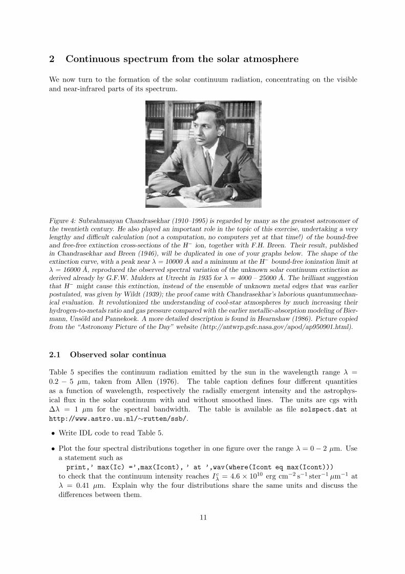
We now turn to the formation of the solar continuum radiation, concentrating on the visibleand near-infrared parts of its spectrum.

Figure 4: Subrahmanyan Chandrasekhar (1910–1995) is regarded by many as the greatest astronomer ofthe twentieth century. He also played an important role in the topic of this exercise, undertaking a verylengthy and difficult calculation (not a computation, no computers yet at that time!) of the bound-freeand free-free extinction cross-sections of the H− ion, together with F.H. Breen. Their result, publishedin Chandrasekhar and Breen (1946), will be duplicated in one of your graphs below. The shape of theextinction curve, with a peak near λ = 10000 A and a minimum at the H− bound-free ionization limit atλ = 16000 A, reproduced the observed spectral variation of the unknown solar continuum extinction asderived already by G.F.W. Mulders at Utrecht in 1935 for λ = 4000 – 25000 A. The brilliant suggestionthat H− might cause this extinction, instead of the ensemble of unknown metal edges that was earlierpostulated, was given by Wildt (1939); the proof came with Chandrasekhar’s laborious quantummechan-ical evaluation. It revolutionized the understanding of cool-star atmospheres by much increasing theirhydrogen-to-metals ratio and gas pressure compared with the earlier metallic-absorption modeling of Bier-mann, Unsold and Pannekoek. A more detailed description is found in Hearnshaw (1986). Picture copiedfrom the “Astronomy Picture of the Day” website (http://antwrp.gsfc.nasa.gov/apod/ap950901.html).

2.1 Observed solar continua

Table 5 specifies the continuum radiation emitted by the sun in the wavelength range λ =0.2 − 5 µm, taken from Allen (1976). The table caption defines four different quantitiesas a function of wavelength, respectively the radially emergent intensity and the astrophys-ical flux in the solar continuum with and without smoothed lines. The units are cgs with∆λ = 1 µm for the spectral bandwidth. The table is available as file solspect.dat athttp://www.astro.uu.nl/∼rutten/ssb/.

• Write IDL code to read Table 5.

• Plot the four spectral distributions together in one figure over the range λ = 0 − 2 µm. Usea statement such as

print,’ max(Ic) =’,max(Icont), ’ at ’,wav(where(Icont eq max(Icont)))

to check that the continuum intensity reaches I cλ = 4.6 × 1010 erg cm−2 s−1 ster−1 µm−1 at

λ = 0.41 µm. Explain why the four distributions share the same units and discuss thedifferences between them.

11

• Convert these spectral distributions into values per frequency bandwidth ∆ν = 1 Hz. Plotthese also against wavelength. Check: peak I c

ν = 4.21 × 10−5 erg cm−2 s−1 ster−1 Hz−1 atλ = 0.80 µm.

• Write an IDL function planck.pro (or use your routine from Exercises “Stellar Spectra A:Basic Line Formation”, or use mine) that computes the Planck function in the same units.Try to fit a Planck function to the solar continuum intensity. What rough temperatureestimate do you get?

• Invert the Planck function analytically to obtain an equation which converts an intensitydistribution Iλ into brightness temperature Tb (defined by Bλ(Tb) ≡ Iλ). Code it as anIDL function and use that to plot the brightness temperature of the solar continuum againstwavelength (with the plot,/ynozero keyword). Discuss the shape of this curve. It peaksnear λ = 1.6 µm. What does that mean for the radiation escape at this wavelength?

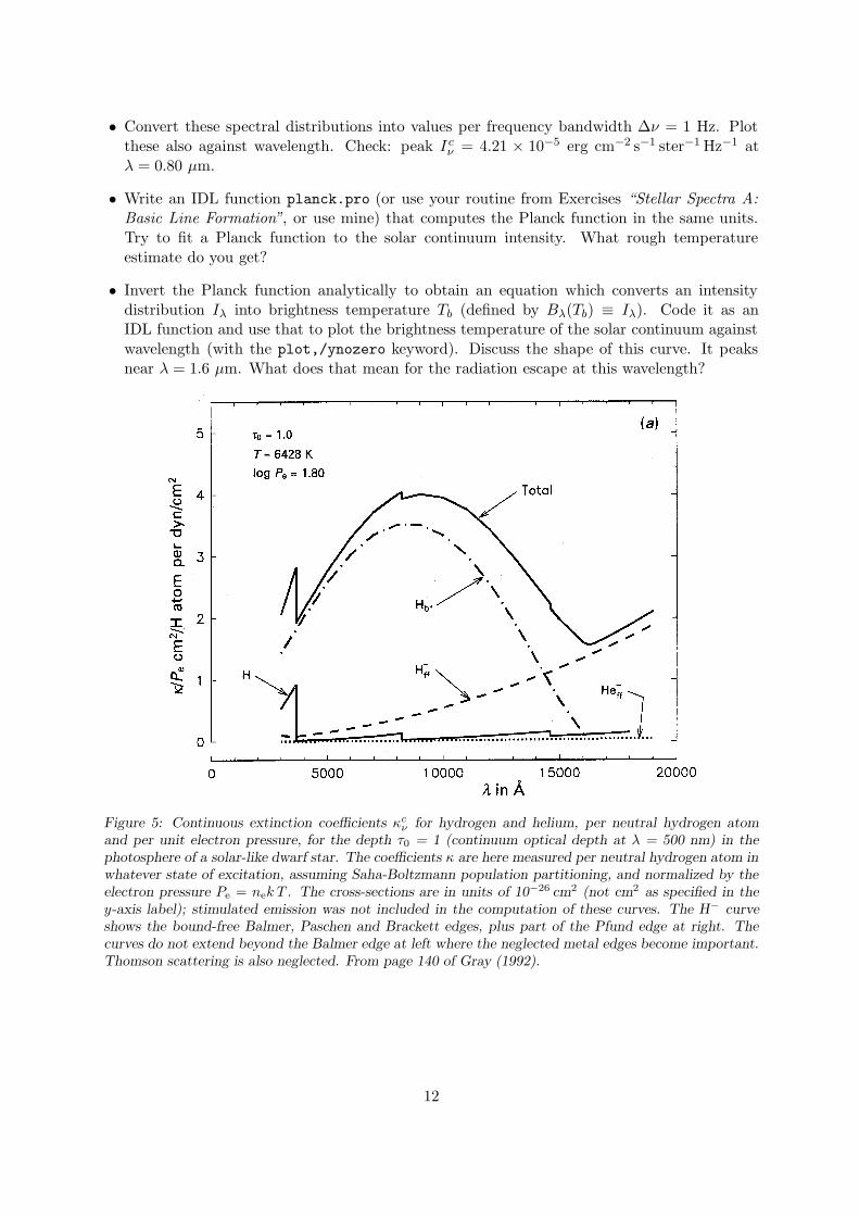
Figure 5: Continuous extinction coefficients κcν for hydrogen and helium, per neutral hydrogen atom

and per unit electron pressure, for the depth τ0 = 1 (continuum optical depth at λ = 500 nm) in thephotosphere of a solar-like dwarf star. The coefficients κ are here measured per neutral hydrogen atom inwhatever state of excitation, assuming Saha-Boltzmann population partitioning, and normalized by theelectron pressure Pe = nek T . The cross-sections are in units of 10−26 cm2 (not cm2 as specified in they-axis label); stimulated emission was not included in the computation of these curves. The H− curveshows the bound-free Balmer, Paschen and Brackett edges, plus part of the Pfund edge at right. Thecurves do not extend beyond the Balmer edge at left where the neglected metal edges become important.Thomson scattering is also neglected. From page 140 of Gray (1992).

12

Figure 6: Ionization edges for a selection of abundant elements. The triangular symbols depict bound-free continuum edges in the form of schematic hydrogenic ν−3 decay functions above each ionizationthreshold. The plot shows the edge distribution over ionization energy χ1c (along the bottom) or thresholdwavelength (along the top) and the logarithmic product of the element abundance A12 ≡ log(nE/nH +12) and the bound-free cross-section per particle at threshold σ/σH (vertically). Thus, it shows therelative importance of the major bound-free edges throughout the spectrum. They are all at ultravioletwavelengths and do not contribute extinction in the visible and infrared. The plus signs indicate importantfirst-ion edges; higher ionization stages produce edges at yet shorter wavelengths. The abundance valuescome from Engvold (1977), the ionization energies from Novotny (1973), the cross-sections from Baschekand Scholz (1982). Thijs Krijger production following unpublished lecture notes by E.H. Avrett, takenfrom the lecture notes available at http://www.astro.uu.nl/∼rutten.

2.2 Continuous extinction

We will assume that H−

(a hydrogen atom with an extra electron) is the major provider ofcontinuous extinction in the solar atmosphere. This is quite a good assumption for the solarphotosphere for wavelengths λ > 0.5 µm (5000 A). The second-best extinction provider are H Ibound-free interactions, at only a few percent. This may be seen in Figure 5 taken from Gray(1992).

Below λ = 500 nm there is heavy line crowding (not added in Figure 5) which acts as a quasi-continuum. Below λ = 365 nm the Balmer bound-free edge provides large extinction, and atyet shorter wavelengths the bound-free ionizaton edges of various metals (Al I, Mg I, Fe I, Si I,C I) provide steep extinction increase yet before the H I Lyman continuum sets is, as may beexpected from Figure 6. In this exercise we will neglect these contributions by evaluating onlythe H

−

extinction and the extinction due to scattering off free electrons (Thomson scattering).

IDL function exthmin.pro evaluates polynomial fits for H−

extinction that are given onpage 135 ff of Gray (1992). The routine delivers the total (bound-free plus free-free) H

−

ex-

13

tinction in units of cm2 per neutral hydrogen atom (not per H−

ion!). LTE is assumed in thecomputation of the H

−

ion density relative to the neutral hydrogen density (through a Sahaequation where the neutral atom takes the place of the ionized state, see page 135 of Gray1992).

• Pull exthmin.pro over and compare it to Gray’s formulation.

• Plot the wavelength variation of the H−

extinction for the FALC parameters at h = 0 km (seeTables 3–4). This plot reproduces the result of Chandrasekhar and Breen (1946). Compareit to Gray’s version in Figure 5.

• Hydrogenic bound-free edges behave just as H I with maximum extinction at the ionizationlimit and decay ∼ λ3 for smaller wavelengths, as indeed shown by the H I curve in Figure 5.The H

−

bound-free extinction differs strongly from this pattern. Why is it not hydrogenicalthough due to hydrogen?

• How should you plot this variation to make it look like the solar brightness temperaturevariation with wavelength? Why?

• Read in the FALC model atmosphere (copy the reading code in readfalc.idl into your IDLprogram). Note that the column nH in the FALC model of Tables 3–4 is the total hydrogendensity, summing neutral atoms and free protons (and H2 molecules but those are virtuallyabsent). This is seen by inspecting the values of nH and np at the top of the FALC tablewhere all hydrogen is ionised. Gray’s H

−

extinction is measured per neutral hydrogen atom,so you have to multiply the height-dependent result from exthmin(wav,temp,eldens) withnneutral H ≈ nH(h) − np(h) to obtain extinction αλ(H

−

) measured per cm path length (orcross-section per cubic cm) at every height h. Plot the variation of the H

−

extinction per cmwith height for λ = 0.5 µm. This plot needs to be logarithmic in y, why?

• Now add the Thomson scattering off free electrons to the extinction per cm. The Thomsoncross-section per electron is the same at all wavelengths and is given by

σT = 6.648 × 10−25 cm2. (5)

With which height-dependent quantity do you have to multiply this number to obtain ex-tinction per cm? Overplot this contribution to the continuous extinction αc

λ(h) in your graphand then overplot the total continuous extinction too. Explain the result.

2.3 Optical depth

Knowing the stratification (FALC model) and the continuous extinction as function of height,we may now compute the corresponding optical depth scale given by:

τλ(h0) ≡ −∫ h0

∞

αcλ dh (6)

at any height h0. Note that FALC is tabulated in reverse order, corresponding to the −hdirection. The IDL library routine INT TABULATED supplies a closed five-point Newton-Cotes integration routine that might be applied, but I found that the simple trapezium rulegives nearly identical results. (It is often much safer to use trapezoidal integration than higher-order schemes. The latter may give wildly wrong answers by fitting the samples with large

14

excursions in between samples. A good recipe is to always stick to trapezoidal integration andto refine the grid if higher precision is desired.)

• Integrate the extinction at λ = 500 nm to obtain the τ500 scale and compare it graphicallyto the FALC τ500 scale. Here is my code, with ext(ih) denoting the continuous extinctionper cm at λ = 500 nm and at height h(ih):

; compute and plot tau at 500 nm, compare with FALC tau5

tau=fltarr(nh)

for ih=1,nh-1 do tau(ih)=tau(ih-1)+$

0.5*(ext(ih)+ext(ih-1))*(h(ih-1)-h(ih))*1E5

plot,h,tau,/ylog,$

xtitle=’height [km]’,ytitle=’tau at 500 nm’

oplot,h,tau5,linestyle=2

2.4 Emergent intensity and height of formation

We are now ready to compute the intensity of the radiation that emerges from the center of thesolar disk (in the radial direction from the solar sphere). It is given (assuming plane-parallelstratification) by:

Iλ =

∫

∞

0Sλ e−τλ dτλ. (7)

It is interesting to also inspect the intensity contribution function

dIλ

dh= Sλ e−τλαλ (8)

which shows the relative contribution of each layer to the emergent intensity. Its weighted meandefines the “mean height of formation”:

<h>≡∫

∞

0 h (dIλ/dh) dh∫

∞

0 (dIλ/dh) dh=

∫

∞

0 hSλ e−τλ dτλ∫

∞

0 Sλ e−τλ dτλ. (9)

Here is my code to compute and diagnose these quantities for a given wavelength (wl in µm)assuming LTE and using trapezoidal integration:

; emergent intensity at wavelength wl (micron)

ext=fltarr(nh)

tau=fltarr(nh)

integrand=fltarr(nh)

contfunc=fltarr(nh)

int=0.

hint=0.

for ih=1,nh-1 do begin

ext(ih)=exthmin(wl*1E4,temp(ih),nel(ih))*(nhyd(ih)-nprot(ih))$

+0.664E-24*nel(ih)

tau(ih)=tau(ih-1)+0.5*(ext(ih)+ext(ih-1))*(h(ih-1)-h(ih))*1E5

integrand(ih)=planck(temp(ih),wl)*exp(-tau(ih))

15

int=int+0.5*(integrand(ih)+integrand(ih-1))*(tau(ih)-tau(ih-1))

hint=hint+h(ih)*0.5*(integrand(ih)+integrand(ih-1))*(tau(ih)-tau(ih-1))

contfunc(ih)=integrand(ih)*ext(ih)

endfor

hmean=hint/int

• The code above sits in file emergint.idl. Copy it into your IDL program and make it worksetting wl=0.5.

• Compare the computed intensity at λ = 500 nm with the observed intensity, using a statementsuch as

print,’ observed cont int = ’,Icont(where(wl eq wav))

to obtain the latter.

• Plot the contribution function against height and compare its peak location with the meanheight of formation.

• Repeat the above for λ = 1 µm, λ = 1.6 µm, and λ = 5 µm. Discuss the changes of thecontribution functions and their cause.

• Check the validity of the LTE Eddington-Barbier approximation Iλ ≈ Bλ(T [τλ = 1]) bycomparing the mean heights of formation with the τλ = 1 locations and with the locationswhere Tb = T (h).

2.5 Disk-center intensity

The solar disk-center intensity spectrum can now be computed by repeating the above in a bigloop over wavelength.

• Compute the emergent continuum over the wavelength range of Table 5.

• Compare it graphically with the observed solar continuum in Table 5 and file solspect.dat.

2.6 Limb darkening

The code is easily modified to give the intensity that emerges under an angle µ = cos θ, inplane-parallel approximation given by:

Iλ(0, µ) =

∫

∞

0Sλ e−τλ/µ dτλ/µ. (10)

• Repeat the intensity evaluation using (10) within an outer loop over µ = 0.1, 0.2, . . . , 1.0.

• Plot the computed ratio Iλ(0, µ)/Iλ(0, 1) at a few selected wavelengths, against µ and alsoagainst the radius of the apparent solar disk r/R = sin θ. Explain the limb darkening andits variation with wavelength.

16

2.7 Flux integration

The emergent intensity may now be integrated over emergence angle to get the emergent astro-physical flux:

Fλ(0) = 2

∫ 1

0Iλ(0, µ)µ dµ. (11)

The problem arises that (10) cannot be evaluated at µ = 0. The naive way to get F is simplyto integrate Iλ(0, µ) trapezoidally over the ten angles µ = 0.1, 0.2, . . . , 1.0 at which you have italready, but that produces too much flux by ignoring the relatively low contribution from theouter limb (µ = 0.0 − 0.1, sin θ = 0.995 − 1.0). This integral is therefore better evaluated with“open quadrature”, an integration formula neglecting the endpoints. Classical equal-spacingrecipes are the Open Newton-Cotes quadrature formulae but it is much better to use non-equidistant Gaussian quadrature (see the chapter “Integration of functions” in Numerical Recipesby Press et al. 1986). The defining formula is:

∫ +1

−1f(x) dx ≈

n∑

i=1

wi f(xi) (12)

and the required abscissa values xi and weights wi are tabulated for n = 2− 10 and even higherorders on page 916 of Abramowitz and Stegun (1964). Three-point Gaussian integration issufficiently accurate for the emergent flux integration.

• Compute the emergent solar flux and compare it to the observed flux in Table 5 and filesolspect.dat. Here is my code (file gaussflux.idl):

; ===== three-point Gaussian integration intensity -> flux

; abscissae + weights n=3 Abramowitz & Stegun page 916

xgauss=[-0.7745966692,0.0000000000,0.7745966692]

wgauss=[ 0.5555555555,0.8888888888,0.5555555555]

fluxspec=fltarr(nwav)

intmu=fltarr(3,nwav)

for imu=0,2 do begin

mu=0.5+xgauss(imu)/2. ; rescale xrange [-1,+1] to [0,1]

wg=wgauss(imu)/2. ; weights add up to 2 on [-1,+1]

for iw=0,nwav-1 do begin

wl=wav(iw)

@emergintmu.idl ; old trapezoidal integration I(0,mu)

intmu(imu,iw)=int

fluxspec(iw)=fluxspec(iw)+wg*intmu(imu,iw)*mu

endfor

endfor

fluxspec=2*fluxspec ; no !pi, AQ has flux F, not \cal F

plot,wav,fluxspec,$

xrange=[0,2],yrange=[0,5E10],$

xtitle=’wavelength [micron]’,ytitle=’solar flux’

oplot,wav,Fcont,linestyle=2

xyouts,0.5,4E10,’computed’

xyouts,0.35,1E10,’observed’

17

2.8 Discussion

You have succeeded in explaining the solar continuum at visible and infrared wavelengths aslargely due to H

−

extinction. This is what Chandrasekhar and Breen (1946) accomplished afterWildt (1939) suggested that H

−

might be the long-sought source of photospheric extinction.The bound-free contribution from H I is small since the required populations of n = 3 (Paschencontinuum) and n = 4 (Brackett continuum) are small (Boltzmann partitioning; cf. Figure 5).Other elements do not contribute continuous extinction in the visible and infrared because theirmajor bound-free edges are all in the ultraviolet (Figure 6).

The large opacity of the solar photosphere is therefore due to the combination of abundantneutral hydrogen atoms, the presence of free electrons (that come mostly from other particlespecies with lower ionization energy), and the large polarization of the simple electron-protoncombination which produces a large cross-section for Coulomb interactions between hydrogenatoms and free electrons. There are no free electrons in our own atmosphere and the moleculesmaking up the air around us possess much better Coulomb shielding; terrestrial air is therefore farless opaque at visible wavelengths than the solar gas. In the infrared, air is similarly transparantin some spectral windows correspondig to energy bands in which the molecules can’t rotate orvibrate.

In general, radiative transfer in stellar atmospheres is a difficult subject because in our dailyphysical experience, gases ought to be transparent. Even though stars are fully gaseous, they arefar from transparent. H

−

extinction makes even the atmospheres of cool stars less transparentthan what we would expect for gases so tenuous.

A final note: while LTE is an excellent assumption for H−

bound-free processes and exactlyvalid (as long as the Maxwell distribution holds) for H

−

free-free processes, it is not at allvalid for Thomson scattering. The process source function for purely coherent (monochromatic)scattering is not given by Bλ(T ) but by the angle-averaged intensity Jλ ≡ (1/4π)

∫

Iλ dΩ.Obtaining Jλ from such an integration requires knowledge of the intensity Iλ(h, θ) locally andin all directions θ, not just the emergent one at τ = 0 computed here. This evaluation willbe treated extensively in exercises “Stellar Spectra C: NLTE Line Formation”. For now, suchsophistication is too much work, and in any case Thomson scattering is not important for theformation of the solar continuum intensity in this wavelength range (as you can see by deleting ordoubling its contribution in your code). However, Thomson scattering dominates the continuousextinction in the photospheres of hot stars in which hydrogen is largely ionized so that the H

−

contribution vanishes while the electron contribution rises.

18

Table 5: Solar spectral distribution, from Allen (1976). Fλ = astrophysical flux at the solar surface withspectral irregularities smoothed; F ′

λ= astrophysical flux at the solar surface for the continuum between

lines; Iλ = radially emergent intensity at the solar surface with spectral irregularities smoothed; I ′

λ=

radially emergent intensity at the solar surface for the continuum between lines. “Astrophysical” flux Fλ

is defined as π Fλ ≡ Fλ with Fλ the net outward flow of energy through a stellar surface element. Theastrophysical flux is often prefered because it has Fλ =< Iλ > with < Iλ > the intensity averaged overthe stellar disk received by a distant observer. It has the same dimension as intensity, whereas Fλ is notmeasured per steradian.

λ Fλ F ′

λ Iλ I ′

λ

µm 1010 erg cm−2 s−1 µm−1 ster−1

0.20 0.02 0.04 0.03 0.04

0.22 0.07 0.11 0.14 0.20

0.24 0.09 0.2 0.18 0.30

0.26 0.19 0.4 0.37 0.5

0.28 0.35 0.7 0.59 1.19

0.30 0.76 1.36 1.21 2.15

0.32 1.10 1.90 1.61 2.83

0.34 1.33 2.11 1.91 3.01

0.36 1.46 2.30 2.03 3.20

0.37 1.57 2.50 2.33 3.62

0.38 1.46 2.85 2.14 4.1

0.39 1.53 3.10 2.20 4.4

0.40 2.05 3.25 2.9 4.58

0.41 2.46 3.30 3.43 4.60

0.42 2.47 3.35 3.42 4.59

0.43 2.46 3.36 3.35 4.55

0.44 2.66 3.38 3.58 4.54

0.45 2.90 3.40 3.86 4.48

0.46 2.93 3.35 3.88 4.40

0.48 2.86 3.30 3.73 4.31

0.50 2.83 3.19 3.63 4.08

0.55 2.72 2.94 3.40 3.68

0.60 2.58 2.67 3.16 3.27

0.65 2.31 2.42 2.78 2.88

0.70 2.10 2.13 2.50 2.53

0.75 1.88 1.91 2.22 2.24

0.8 1.69 1.70 1.96 1.97

0.9 1.33 1.36 1.53 1.55

1.0 1.08 1.09 1.21 1.23

1.2 0.73 0.74 0.81 0.81

1.4 0.512 0.512 0.564 0.564

1.6 0.375 0.375 0.403 0.403

1.8 0.248 0.248 0.268 0.268

2.0 0.171 0.171 0.183 0.183

2.5 0.0756 0.0756 0.081 0.081

3.0 0.0386 0.0386 0.041 0.041

4.0 0.0130 0.0130 0.0135 0.0135

5.0 0.0055 0.0055 0.0057 0.0057

19

20

3 Spectral lines from the solar atmosphere

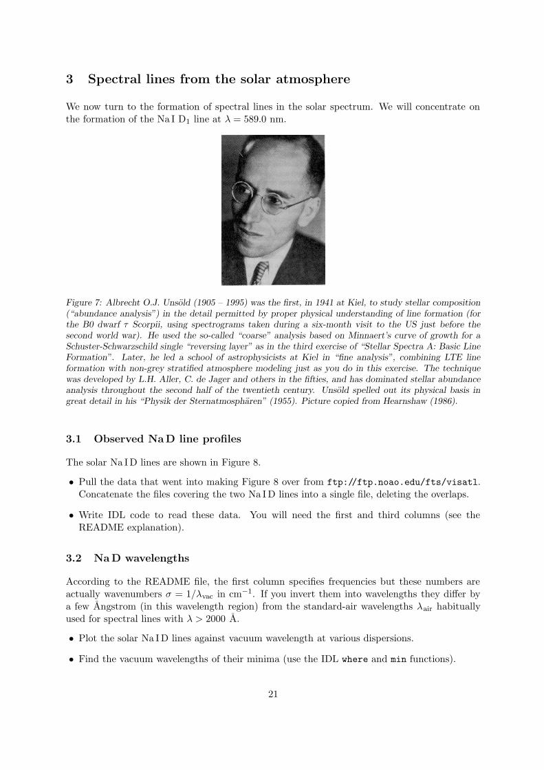
We now turn to the formation of spectral lines in the solar spectrum. We will concentrate onthe formation of the Na I D1 line at λ = 589.0 nm.

Figure 7: Albrecht O.J. Unsold (1905 – 1995) was the first, in 1941 at Kiel, to study stellar composition(“abundance analysis”) in the detail permitted by proper physical understanding of line formation (forthe B0 dwarf τ Scorpii, using spectrograms taken during a six-month visit to the US just before thesecond world war). He used the so-called “coarse” analysis based on Minnaert’s curve of growth for aSchuster-Schwarzschild single “reversing layer” as in the third exercise of “Stellar Spectra A: Basic LineFormation”. Later, he led a school of astrophysicists at Kiel in “fine analysis”, combining LTE lineformation with non-grey stratified atmosphere modeling just as you do in this exercise. The techniquewas developed by L.H. Aller, C. de Jager and others in the fifties, and has dominated stellar abundanceanalysis throughout the second half of the twentieth century. Unsold spelled out its physical basis ingreat detail in his “Physik der Sternatmospharen” (1955). Picture copied from Hearnshaw (1986).

3.1 Observed NaD line profiles

The solar Na ID lines are shown in Figure 8.

• Pull the data that went into making Figure 8 over from ftp://ftp.noao.edu/fts/visatl.Concatenate the files covering the two Na ID lines into a single file, deleting the overlaps.

• Write IDL code to read these data. You will need the first and third columns (see theREADME explanation).

3.2 Na D wavelengths

According to the README file, the first column specifies frequencies but these numbers areactually wavenumbers σ = 1/λvac in cm−1. If you invert them into wavelengths they differ bya few Angstrom (in this wavelength region) from the standard-air wavelengths λair habituallyused for spectral lines with λ > 2000 A.

• Plot the solar Na ID lines against vacuum wavelength at various dispersions.

• Find the vacuum wavelengths of their minima (use the IDL where and min functions).

21

Figure 8: A page out of the solar disk-center intensity atlas of Wallace et al. (1998). The intensity scale(vertical) is in relative units, normalized to the local continuum intensity between the lines. The lowerhorizontal scales specify wavenumbers in cm−1, the upper ones vacuum wavelengths in A. The atlaswas made with the Fourier Transform Spectrometer at the McMath-Pierce solar telescope at Kitt Peak(Brault 1978). Telluric lines have been removed. Both the atlas pages and the input data are availableat ftp://ftp.noao.edu/fts/visatl.

• Check that the Na ID wavelengths tabulated in the solar spectrum line list of Mooreet al. (1966) (computer-readable at ftp://ftp.noao.edu/fts/linelist/Moore) are λ =5895.94 A for Na I D1 and λ = 5889.97 A for Na I D2, respectively. Check the identificationof a few blends (other lines) in Figure 8 with the entries in this table2.

• The Astrolib3 routines airtovac and vactoair convert air into vacuum wavelengths andvice versa. A reasonably accurate transformation is also given by

λair = 0.99972683λvac + 0.0107 − 196.25/λvac (13)

with both λ’s in A, from Neckel (1999)4. Use this equation or routine vactoair to plot the

2The solar spectrum line list was constructed at Utrecht. All equivalent widths were measured by hand,

hard labour for many during two decades. The line identifications were made from laboratory wavelength tables

compiled by Mrs. Charlotte Moore and co-workers at the US National Bureau of Standards.3IDL astrolib at http://idlastro.gsfc.nasa.gov/homepage.html/.4This publication is the announcement of two solar atlases, respectively for disk-averaged and disk-center

intensity, constructed from the same FTS data from which the NSO atlases were made. These also specify absolute

intensities. They are available through anonymous ftp at ftp.hs.uni-hamburg.de, /pub/outgoing/FTS.

22

Na ID lines against air wavelength.

3.3 LTE line formation

We will now compute the solar Na I D1 line assuming the FALC model atmosphere and LTE forthe line source function. Since LTE holds already for the continuum processes at these wave-lengths (being dominated by H

−

bound-free transitions), the assumption of LTE line formationimplies that you can simply set S l

λ = Scλ = Stotal

λ = Bλ(T ). What remains is first to evaluate theline extinction as a function of height and wavelength, and then to add that to the continuousextinction in the integration loop of the previous exercise. The outer loop over wavelength thenhas to sample the Na ID1 profile (but not as finely as the atlas data spacing).

3.4 Line extinction

The monochromatic line extinction per cm path lenght for a bound-bound transition between alower level l and an upper level u is given by:

αlλ =

√πe2

mec

λ2

cbl

nLTEl

NENH AE flu

H(a, v)

∆λD

[

1 − bu

ble−hc/λkT

]

, (14)

which holds generally when the line broadening is described by the Voigt function H(a, v), avalid assumption for the Na ID lines (but wrong for hydrogen lines which are broadened with theHoltsmark distribution). For LTE the population departure coefficients of the lower and upperlevels are bl = bu = 1. The LTE population fraction nLTE

l /NE (lower level population scaled bythe total element population) is given by the combined Saha and Boltzmann distributions

Ur ≡∑

s

gr,s e−χr,s/kT (15)

nr,s

Nr=

gr,s

Ure−χr,s/kT (16)

Nr+1

Nr=

1

Ne

2Ur+1

Ur

(

2πmekT

h2

)3/2

e−χr/kT , (17)

where s is the level counter and r the ionization stage counter.

Some numbers for the Na I D1 and Na I D2 lines:

– sodium ionization energies χ1 = 5.139 eV, χ2 = 47.29 eV, χ3 = 71.64 eV (Appendix D ofGray 1992);

– the Na I D1 and Na I D2 lower-level excitation energy χ1,1 = 0 eV (shared ground state);

– the Na I D1 and Na I D2 lower-level statistical weight g1,1 = 2 (ground state 3s 2S1/2, g =2J + 1);

– the oscillator strengths are flu = 0.318 for Na I D1, flu = 0.631 for Na I D2;

– the Na I partition function defined by (15) is given in Appendix D of Gray (1992) aslog UNa I(T ) ≈ c0 +c1 log θ+c2 log2 θ+c3 log3 θ+c4 log4 θ with θ ≡ 5040./T and c0 = 0.30955,c1 = −0.17778, c2 = 1.10594, c3 = −2.42847 and c4 = 1.70721;

– the Na II and Na III partition functions are well approximated by the statistical weights ofthe ion ground states, respectively UNa II = 1, UNa III = 6 (Allen 1976);

– the sodium abundance is ANa = NNa/NH = 1.8 × 10−6 (Allen 1976).

23

3.5 Line broadening

The Voigt function H(a, v) describes the extinction profile shape and is defined by:

H(a, v) ≡ a

π

∫ +∞

−∞

e−y2

(v − y)2 + a2dy (18)

y =ξ

c

λ0

∆λD(19)

v =λ − λ0

∆λD(20)

a =λ2

4πc

γ

∆λD, (21)

where ξ is velocity along the line of sight and a the damping parameter. The Dopplerwidth∆νD is not only set by the thermal broadening but includes also the microturbulent “fudgeparameter” vt (column vt in FALC Tables 3–4) through defining it as:

∆λD ≡ λ0

c

√

2kT

m+ v2

t (22)

where m is the mass of the line-causing particle in gram, for sodium mNa = 22.99 × 1.6605 ×10−24 g (http://physics.nist.gov/cuu/Constants/).

The Voigt function represents the convolution (smearing) of a Gauss profile with a Lorentzprofile and therefore has a Gaussian shape close to line center (v = 0) due to the thermalDoppler shifts (“Doppler core”) and extended Lorentzian wings due to disturbances by otherparticles (“damping wings”). A reasonable approximation is obtained by taking the sum ratherthan the convolution of the two profiles:

H(a, v) ≈ e−v2

+a√π v2

. (23)

The area-normalized version

V (a, v) ≡ 1

∆λD

√π

H(a, v) (24)

is available in IDL as function VOIGT(a,v) but it works correctly only for positive v, so use itwith abs(v).

The damping parameter a may be approximated by taking only Van der Waals broadening intoaccount in (21). Figure 11.6 of Gray (1992) shows this by comparing Van der Waals broadeningwith natural broadening and Stark broadening for the Na ID lines throughout a solar model.The classical evaluation recipe of Van der Waals broadening by Unsold (1955) is (cf. Warner1967):

log γvdW ≈ 6.33 + 0.4 log(r2u − r2

l ) + log Pg − 0.7 log T, (25)

where the mean square radii r2 of the upper and lower level are usually estimated from thehydrogenic approximation of Bates and Damgaard (1949)

r2 =n∗2

2Z2

(

5n∗2 + 1 − 3l(l + 1))

(26)

24

with r2 measured in atomic units, l the angular quantum number of the level and n∗ its effective(hydrogen-like) principal quantum number given by

n∗2 = RZ2

E∞ − En(27)

in which the Rydberg constant R = 13.6 eV = 2.18× 10−11 erg, Z is the ionization stage (Z = 1for Na I, Z = 2 for Na II, etc) and E∞−En is the ionization energy from the level (compute theexcitation energy of the upper level from the line-center wavenumber). The common Na I D1

and Na I D2 lower level (3s 2S1/2) has l = 0, the upper levels (3p 2PO

1/2 and 3p 2PO

3/2) have l = 1.

3.6 Implementation

• Split the above equations modularly in IDL functions, for example:parfunc_Na(temp)

saha_Na(temp,eldens,chi_ion)

boltz_Na(temp,chi_level)

sahaboltz_Na(temp,eldens,chi_ion,chi_level)

dopplerwidth(wav,temp,vmicro,atmass)

gammavdw(temp,pgas,ru,rl)

rsq(r,l,chi_ion.chi_level).

• Combine calls of these functions into one that returns the Na I D1 line extinction, for exampleNaD1_ext(wav,temp,eldens,nhyd,vmicro).

3.7 Computed NaD1 line profile

You are now ready to model the solar Na I D1 line.

• Add the Na I D1 line extinction to the continuous extinction in your integration code fromthe previous exercise and compute the disk-center Na I D1 profile.

• Compare the computed line profile to the observed line profile and discuss the differences.Explain why your computed profile has a line-center reversal.

• Traditionally, stellar abundance determiners vary a collisional enhancement factor E by whichγvdW is multiplied in ad-hoc fashion in order to obtain a better fit of the line wings. Try thesame5.

3.8 Discussion

Your code constitutes a 1960–style solar line synthesis program which is actually quite good forphotospheric lines and is easily generalized to other atomic species. However, your computedNa I D1 line core doesn’t reach as deep as the observed one which does not show an intensityreversal. Its bad reproduction shows that the assumption of LTE breaks down for the core ofthis line. No wonder, the solar Na ID lines are strong scatterers (small ε) with large NLTEsource function sensitivity to Jλ rather than to Bλ at heights around and above the temperature

5A better recipe than the classical Unsold one is now available for lines of neutral stages from Paul Barklem

at http://www.astro.uu.se/∼barklem/.

25

minimum where their cores originate. In fact, their formation closely follows the two-level atomdescription for resonance scattering in which both Jλ and Sλ drop down to a value of only about√

εBλ at the surface, displaying standard NLTE scattering behavior. Thus, it is time to turnto the sequel exercises “Stellar Spectra C: NLTE Line Formation” in which you will apply moreadvanced numerical techniques permitting deviations from LTE.

26

References

Abramowitz, M. and Stegun, I.: 1964, Handbook of Mathematical Functions, U.S. Dept. ofCommerce, Washington

Allen, C. W.: 1976, Astrophysical Quantities, Athlone Press, Univ. London

Anders, E. and Grevesse, N.: 1989, Geochim. Cosmochim. Acta 53, 197

Baschek, B. and Scholz, M.: 1982, in K.-H. Hellwege (Ed.), Landolt-Bornstein New Series, Starsand Star Clusters, Group VI Vol. 2b, Astronomy and Astrophysics, Springer, Heidelberg,p. 91

Bates, D. R. and Damgaard, A.: 1949, Phil. Trans. R. Soc. London 242, 101

Brault, J. W.: 1978, in G. Godoli, G. Noci, and A. Righini (Eds.), Future solar optical observa-tions: needs and constraints, Procs. JOSO Workshop, Osservazioni e Memorie Oss. Astrof.Arcetri, Florence, p. 33

Chandrasekhar, S. and Breen, F.: 1946, Astrophys. J. 104, 430

Eddington, A. S.: 1926, The Internal Constitution of the Stars, Dover Pub., New York

Engvold, O.: 1977, Physica Scripta 16, 48

Fontenla, J. M., Avrett, E. H., and Loeser, R.: 1993, Astrophys. J. 406, 319

Gray, D. F.: 1992, The Observation and Analysis of Stellar Photospheres, Cambridge Univ.Press, U.K. (second edition)

Hearnshaw, J. B.: 1986, The analysis of starlight. One hundred and fifty years of astronomicalspectroscopy , Cambridge Univ. Press, Cambridge UK

Moore, C. E., Minnaert, M. G. J., and Houtgast, J.: 1966, The Solar Spectrum 2935 A to8770 A. Second Revision of Rowland’s Preliminary Table of Solar Spectrum Wavelengths,NBS Monograph 61, National Bureau of Standards, Washington

Neckel, H.: 1999, Solar Phys. 184, 421

Novotny, E.: 1973, Introduction to stellar atmospheres and interiors, Oxford Univ. Press, NewYork

Parker, E. N.: 1958, Astrophys. J. 128, 664

Press, W. H., Flannery, B. P., Teukolsky, S. A., and Vetterling, W. T.: 1986, Numerical Recipes,Cambridge Univ. Press, Cambridge UK

Strassmeier, K. G. and Linsky, J. L. (Eds.): 1996, Stellar surface structure, Proc. IAU Symp.176, Kluwer, Dordrecht

Ulrich, R. K.: 1970, Astrophys. J. 162, 933

Unsold, A.: 1955, Physik der Sternatmospharen, Springer Verlag, Berlin (second edition)

Vernazza, J. E., Avrett, E. H., and Loeser, R.: 1981, Astrophys. J. Suppl. Ser. 45, 635

Wallace, L., Hinkle, K., and Livingston, W.: 1998, An Atlas of the Spectrum of the Solar Pho-tosphere from 13,500 to 28,000 cm−1 (3570 to 7405 A), Technical Report 98-001, NationalSolar Observatory, Tucson

Warner, B.: 1967, Mon. Not. R. Astron. Soc. 136, 381

Wildt, R.: 1939, Astrophys. J. 89, 295

27