STELLAR SPECTRA

A. Basic Line Formation

R.J. Rutten

Sterrekundig Instituut Utrecht

May 9, 2003

Copyright c© 1999 Robert J. Rutten, Sterrekundig Instuut Utrecht, The Netherlands.Copying permitted exclusively for non-commercial educational purposes, courtesy of the Euro-pean Solar Magnetometry Network (http://www.astro.uu.nl/∼rutten/tmr).

Contents

Introduction 1

1 Spectral classification(“Annie Cannon”) 31.1 Stellar spectra morphology . . . . . . . . . . . . . . . . . . . . . . . . . . . . . . 31.2 Data acquisition and spectral classification . . . . . . . . . . . . . . . . . . . . . . 31.3 Introduction to IDL . . . . . . . . . . . . . . . . . . . . . . . . . . . . . . . . . . 41.4 Introduction to LaTeX . . . . . . . . . . . . . . . . . . . . . . . . . . . . . . . . . 4

2 Saha-Boltzmann calibration of the Harvard sequence(“Cecilia Payne”) 72.1 Payne’s line strength diagram . . . . . . . . . . . . . . . . . . . . . . . . . . . . . 72.2 The Boltzmann and Saha laws . . . . . . . . . . . . . . . . . . . . . . . . . . . . 82.3 Schadee’s tables for schadeenium . . . . . . . . . . . . . . . . . . . . . . . . . . . 122.4 Saha-Boltzmann populations of schadeenium . . . . . . . . . . . . . . . . . . . . 132.5 Payne curves for schadeenium . . . . . . . . . . . . . . . . . . . . . . . . . . . . . 172.6 Discussion . . . . . . . . . . . . . . . . . . . . . . . . . . . . . . . . . . . . . . . . 192.7 Saha-Boltzmann populations of hydrogen . . . . . . . . . . . . . . . . . . . . . . 192.8 Solar Ca+ K versus Hα: line strength . . . . . . . . . . . . . . . . . . . . . . . . . 212.9 Solar Ca+ K versus Hα: temperature sensitivity . . . . . . . . . . . . . . . . . . . 242.10 Hot stars versus cool stars . . . . . . . . . . . . . . . . . . . . . . . . . . . . . . . 24

3 Fraunhofer line strengths and the curve of growth(“Marcel Minnaert”) 273.1 The Planck law . . . . . . . . . . . . . . . . . . . . . . . . . . . . . . . . . . . . . 273.2 Radiation through an isothermal layer . . . . . . . . . . . . . . . . . . . . . . . . 293.3 Spectral lines from a solar reversing layer . . . . . . . . . . . . . . . . . . . . . . 303.4 The equivalent width of spectral lines . . . . . . . . . . . . . . . . . . . . . . . . 333.5 The curve of growth . . . . . . . . . . . . . . . . . . . . . . . . . . . . . . . . . . 35

Epilogue 37

References 38

Brief IDL manual 39

Brief LaTeX manual 46

Text and programs available at http://www.astro.uu.nl/∼rutten/ssa.

Introduction

These three exercises concern the appearance and nature of spectral lines in stellar spectra.Stellar spectrometry laid the foundation of astrophysics in the hands of:

– Wollaston (1802): first observation of spectral lines in sunlight;

– Fraunhofer (1814–1823): rediscovery of spectral lines in sunlight (“Fraunhofer lines”); theirfirst systematic inventory. Also discussions of the spectra of Venus and some stars;

– Herschel (1823): realization that spectral lines must provide information on the constitutionof stellar matter;

– Kirchhoff & Bunsen (1860): absorption lines in stellar spectra are the reverse of emissionlines from the same particle species in laboratory flames. The strength of the absorption is ameasure of the concentration of the species (abundance);

– Pickering plus “harem” (Williamina Fleming, Antonia Maury, Annie Cannon, and a dozenother women): large-scale spectral classification using photographic spectrograms taken withobjective prisms. Annie Cannon classifies over 200 000 spectrograms and fine-tunes the Har-vard spectral classification sequence O – B – A – F – G – K – M. This is a purely morphologicaldivision on the basis of spectral line appearances;

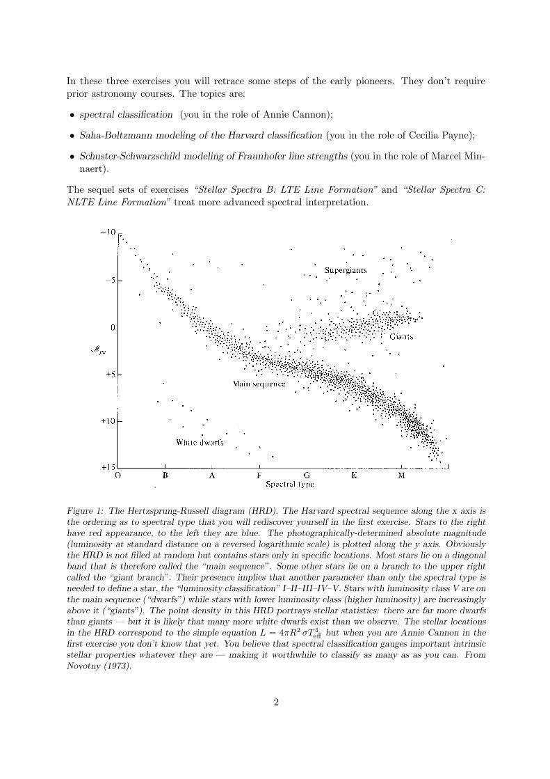
– Hertzsprung (1908) and Russell (1913) independently plot a diagram of stellar absolute mag-nitude against spectral type (Figure 1). It shows that stars occupy sharply defined locationsin this parameter space;

– Cecilia Payne (1925): demonstration that the Saha ionization law explains stellar line strengthvariations. The Harvard spectral sequence is simply a measure of temperature. All starshave about the same chemical composition — not significantly different from the earth’scomposition apart from hydrogen)1;

– Morgan (1938): introduction of the luminosity classification I – II – III – IV – V. This is “theother axis” of the empirical HRD, roughly orthogonal to the main sequence;

– Minnaert and coworkers (1930–1965, Utrecht): introduction of the equivalent width of a lineand the curve of growth for quantitative abundance determination. Detailed inventory ofthe solar spectrum, first graphically in the “Utrecht Atlas” (Minnaert et al. 1940), then intabular form in “The Solar Spectrum 2935A– 8770A” (Moore et al. 1966), listing equivalentwidths for 24 000 Fraunhofer lines;

– Unsold and coworkers (1940-1970, Kiel): precise stellar abundance determinations using LTE(Local Thermodynamic Equilibrium) modeling;

– Schwarzschild, Eddington, Milne, Thomas and many others throughout the twentieth century:development of more general line-formation theory, especially radiation transport throughresonance scattering;

– Avrett, Auer, Mihalas, Hummer, Rybicki and many others, from 1965: application of com-puters to model non-LTE line formation numerically.

1An update of this finding is that the solar composition is the same as that of the oldest meteorites (carbona-ceous chondrites) to very high precision, except for the five lightest elements and carbon. The earth has lost muchof its hydrogen to space, while the sun has burned up 99% of its lithium — fortunately, not more than 6% of itshydrogen yet.

1

In these three exercises you will retrace some steps of the early pioneers. They don’t requireprior astronomy courses. The topics are:

• spectral classification (you in the role of Annie Cannon);

• Saha-Boltzmann modeling of the Harvard classification (you in the role of Cecilia Payne);

• Schuster-Schwarzschild modeling of Fraunhofer line strengths (you in the role of Marcel Min-naert).

The sequel sets of exercises “Stellar Spectra B: LTE Line Formation” and “Stellar Spectra C:

NLTE Line Formation” treat more advanced spectral interpretation.

Figure 1: The Hertzsprung-Russell diagram (HRD). The Harvard spectral sequence along the x axis isthe ordering as to spectral type that you will rediscover yourself in the first exercise. Stars to the righthave red appearance, to the left they are blue. The photographically-determined absolute magnitude(luminosity at standard distance on a reversed logarithmic scale) is plotted along the y axis. Obviouslythe HRD is not filled at random but contains stars only in specific locations. Most stars lie on a diagonalband that is therefore called the “main sequence”. Some other stars lie on a branch to the upper rightcalled the “giant branch”. Their presence implies that another parameter than only the spectral type isneeded to define a star, the “luminosity classification” I–II–III–IV–V. Stars with luminosity class V are onthe main sequence (“dwarfs”) while stars with lower luminosity class (higher luminosity) are increasinglyabove it (“giants”). The point density in this HRD portrays stellar statistics: there are far more dwarfsthan giants — but it is likely that many more white dwarfs exist than we observe. The stellar locationsin the HRD correspond to the simple equation L = 4πR2 σT 4

eff but when you are Annie Cannon in thefirst exercise you don’t know that yet. You believe that spectral classification gauges important intrinsicstellar properties whatever they are — making it worthwhile to classify as many as as you can. FromNovotny (1973).

2

1 Spectral classification

(“Annie Cannon”)

In this exercise you classify stellar spectra without prior knowledge — just as Annie Cannondid while setting up the Harvard sequence O – B – A – F – G – K – M.

Figure 2: Annie Jump Cannon (1863 – 1941) entered Harvard College Observatory in 1886 as an assistantto Edward Pickering, director of Harvard Observatory during 42 years. He was devoted to large-scalestellar spectrometry and set up the monumental “Henry Draper Catalague” of stellar spectra which wasmostly assembled by Annie Cannon and her assistants, funded by a series of gifts from Mrs. Draper whowanted a memorial to her husband, the first spectroscopist to photograph a stellar spectrum (from aprivate observatory on the Hudson River). The effort started in 1886 (Draper died in 1882) and wasconcluded in 1924 with the publication of the 9th volume of the Catalogue in the Harvard Annals. Bythen, Mrs. Draper’s quarter-million dollar bequest had yielded a quarter million stellar classifications.More history of astronomical spectroscopy is found in “The analysis of starlight” by Hearnshaw (1986),from which this photograph is copied.

1.1 Stellar spectra morphology

Figure 3 shows a set of photographic stellar spectrograms. They are rather like the spectrogramsclassified at Harvard. Note that they are negatives; stellar spectra usually contain absorptionlines, dark on a brighter background (the “continuum”).

• Cut the page into strips, one per spectrum, and order them into a morphological sequence.You are the first astronomer studying these spectra and you don’t know what the coding is,except that the lines have something to do with the presence of specific elements.

• Try to explain all you see and speculate on the meaning of your ordering.

1.2 Data acquisition and spectral classification

This is a canned computer exercise for PC’s running Windows taken from:http://www.gettysburg.edu/project/physics/clea/CLEAhome.html.

3

• Get the CLEA-SPEC exercise (file clea.zip at http://www.astro.uu.nl/∼rutten/ssa/).

• Unzip clea.zip and install the CLEA-SPEC exercise.

• Start the exercise.

• Work through the exercise as defined in the Clea-Spec Student Manual, or go through it bysimply clicking on the various options. You should classify a number of stellar spectra. Ifyou prefer taking spectra before classifying them, do the observing first.

1.3 Introduction to IDL

We will use the interactive programming language IDL in the second and third exercise. Usethe remainder of this session to (re-)familiarize yourself with IDL.

• Start IDL.

• Work through the first two pages of the brief IDL manual at the end of this instruction. Youwon’t need the image display routines or the input/output routines in these exercises.

• Write an IDL function ADDUP(array) as the one in the manual in a file ADDUP.PRO and try itout. You will need to put the file in a partition where you have write access, and to redirectIDL to that location (for example through cd,’c:\yourdir\idl\’).

1.4 Introduction to LaTeX

You should write a report in which you include the pertinent graphs made with IDL. You shouldexplain everything seen in the graphs.

If you choose to use LaTeX as text processor (highly recommended if you want to gain experiencein writing reports the astronomer’s way) then:

• Read the brief LaTeX manual at the end of this instruction.

• Copy file http://www.astro.uu.nl/∼rutten/ssa/latex-template.tex to your writing di-rectory. This is a template for your report.

In any case:

• Start writing, and inspect the result.

• Experiment with IDL figure inclusion.

4

61 Cyg A

β Vir

Coma T60

HD 36936

16 Cyg A

γ Uma

HD 95735

HD 36865

78 Uma

HD 37129

Coma T 183

61 Cyg b

45 Boo

σ Dra

β Com

61 Uma

HD 46149

HD 109011

Figure 3: Stellar spectrograms taken with a low-dispersion grating spectrometer. The wavelength in-creases to the right. From Abt et al. (1968).

5

6

2 Saha-Boltzmann calibration of the Harvard sequence

(“Cecilia Payne”)

In this exercise you will explain the spectral-type sequence that is studied morphologically inthe first exercise and that is summarized in Figure 5. You so re-act the work of Cecilia Payne atHarvard. Her 1925 thesis was called “undoubtedly the most brilliant PhD thesis ever writtenin astronomy” by Otto Struve. Its opening sentences are:

“The application of physics in the domain of astronomy constitutes a line of investigation thatseems to possess almost unbounded possibilities. In the stars we examine matter in quantitiesand under conditions unattainable in the laboratory. The increase in scope is counterbalanced,however, by a serious limitation — the stars are not accessible to experiment, only to observation,and there is no very direct way to establish the validity of laws, deduced in the laboratory, whenthey are extrapolated to stellar conditions.”

Extrapolation of terrestrial physics laws is precisely what Payne did in her thesis. She appliedthe newly derived Saha distribution for different ionization stages of an element to stellar spectra,finding that the empirical Harvard classification represents primarily a temperature scale. Herwork crowned efforts of Saha, Russell, Fowler, Milne, Pannekoek and others along the same lines.It illustrates that detailed physics, in this case atomic physics, is usually needed to explain cosmicphenomena.

Figure 4: Cecilia Payne (1900 – 1979) was educated at Cambridge by Milne and Eddington. She went tothe US in 1923 and spent the rest of her career at Harvard (Boston). Her 1925 thesis was the first onein astronomy at Harvard University and remains highly readable as a wide review of stellar spectroscopyat the time. The main conclusion was that stellar composition does not change much from star to star.Russell had already suggested so a decade earlier, but her thesis under Russells’ guidance, published asthe first Harvard Observatory Monograph, brought the point home. Copied from Hearnshaw (1986).

2.1 Payne’s line strength diagram

The key graph in Payne’s thesis (page 131, earlier published in Payne 1924) is reprinted inFigure 6. Clearly, the observed behavior in the upper panel is qualitatively explained by thecomputed behavior in the lower panel. We will recompute the latter.

7

Figure 5: The Harvard spectral sequence. These example spectra are printed positively, with the ab-sorption lines dark on a bright background. Wavelengths in Angstrom (1 A= 0.1 nm = 10−8 cm). Thepeak brightness shifts from left to right from the “early-type” stars (O and B) to the “late-type” stars(G and lower). The sun has spectral type G2V and is a late-type star. The early-type stars display thehydrogen Balmer lines prominently, but these become weak in solar-type spectra in which the Ca+ Hand K resonance lines are strongest. The M dwarfs on the bottom display strong molecular bands. FromNovotny (1973).

2.2 The Boltzmann and Saha laws

In thermodynamical equilibrium (TE) macroscopic equipartition laws hold with the gas tem-perature as the major parameter. These are the Kirchhoff, Planck, Wien and Stefan-Boltzmannlaws for radiation, and the Maxwell, Saha and Boltzmann laws for matter. In this exercisewe are concerned with the latter two. They describe the division of the particles of a specificelement over its different ionization stages and over the discrete energy levels within each stage.For example, the Saha law specifies the distribution of iron particles between neutral iron (Fe),once-ionized iron (Fe+), twice-ionized iron (Fe2+), etc., whereas the Boltzmann law specifiesthe sub-distribution of the iron particles per ionization stage over the discrete energy levels thateach of the Fe, Fe+, Fe2+ etc.2 stages may occupy. Figure 7 illustrates the energy level structureof neutral hydrogen.

Boltzmann law. In TE the partitioning of a specific atom or ion stage over its discrete energylevels (“excitation equilibrium”) is given by the Boltzmann distribution

nr,s

Nr=

gr,s

Ure−χr,s/kT , (1)

2In astronomy one doesn’t write ions as Fe3+ but rather as Fe IV. More precisely: Fe I is the spectrum ofneutral iron Fe, Fe II the spectrum of once-ionized iron Fe+, etc.

8

Figure 6: The strengths of selected lines along the spectral sequence. Upper panel: variations of observedline strengths with spectral type in the Harvard sequence. The latter is plotted in reversed order on anon-linear scale that was obtained by making the peaks coincide with the corresponding peaks in thelower panel. The y-axis units are eye estimates on an arbitrary scale. Lower panel: Saha-Boltzmannpredictions of the fractional concentration Nr,s/N of the lower level of the lines indicated in the upperpanel, each labeled with its ionization stage, on logarithmic y-axis scales that are specified per species atthe bottom, against temperature T along the x axis given in units of 1000 K along the top. The pressurewas taken constant at Pe = Ne k T = 131 dyne cm−2 = 13.1 Pascal. From Novotny (1973) who took itfrom Payne (1924).

with T the temperature, k the Boltzmann constant, nr,s the number of particles per cm3 in levels of ionization stage r, gr,s the statistical weight of that level, and χr,s the excitation energy ofthat level measured from the ground state (r, 1), Nr ≡ ∑

s nr,s the total particle density in alllevels of ionization stage r, and Ur its partition function3 defined by

Ur ≡∑

s

gr,s e−χr,s/kT . (2)

Thus, the neutral stage has r = 1, each ground state is at s = 1, and each ground state hasexcitation energy χr,1 = 0. and ionization energy to the next stage χr. A radiative deexcitationbetween levels (r, s) and (r, t), with level s “higher” than level t, releases a photon with energyχr,s − χr,t = hν = hc/λ, with h the Planck constant, ν the photon frequency, c the velocityof light and λ the wavelength. The excitation energy χr,s is the energy difference between

3Dutch: toestandssom.

9

Figure 7: Energy level diagram for hydrogen. The bound levels are at excitation energies given by (5)on page 19. They approach the ionization threshold at χH = 13.598 eV for n → ∞. The principalquantum number n equals the level counter s in this simple structure. The fine structure of each level(splitting in 2 n2 sublevels) is not shown. For each of the first four hydrogen series the principal bound-bound transitions between bound levels are marked by vertical lines with the name and the wavelengthof the corresponding spectral line. The series limits (n = ∞) are also marked. A bound-free ioniza-tion/recombination transition is added to the Balmer series. The amount of energy above the ionizationthreshold represents the kinetic energy that is gained or lost. A free-free transition (radiative encounterbetween a bare proton and a free electron) is also marked. The bound-free and free-free transitions con-tribute to stellar continua, while the bound-bound transitions produce the hydrogen lines. The Lymanlines are in the ultraviolet, the Balmer lines are in the visible and the Paschen and Brackett lines are inthe infrared. Some Balmer lines are present in the stellar spectrograms in Figure 5. The solar Balmer αline (usually called Hα) is shown in Figure 9. From Novotny (1973).

the excited level (r, s) and the ground state (r, 1). Astronomers usually call it “excitationpotential” and measure it from the ground state up4 in electron volt, with 1 eV correspondingto 1.6022 × 10−12 erg (1.6022 × 10−19 Joule). For example, the H I Balmer α line results fromphotonic transitions between levels n = 2 and n = 3 of neutral hydrogen, with χ1,3 = 12.09 eV,χ1,2 = 10.20 eV and wavelength λ = hc/(χ1,3 − χ1,2) = 656.3 nm (Figure 7).

4Physicists often measure level energies as “binding energy” from the ground state of the next ion down inwavenumbers (cm−1).

10

eV

1

2

3

4

5

6

7

1

2

3

4

5

6

7

16

15

0

1

31

30

0

1

51

50

0

1

22

33 3

2

0

EE

E

E+

2

3

+

+

Schadeenium

s

eVeV

eV

Figure 8: Energy level diagram for Schadee’s element E, showing the neutral stage (lefthand column,r = 1) and the first three ionization stages (r = 2 − 4). The level energies increase in 1 eV steps. Thecolumns may be thought of as being stacked on top of each other since each ion requires the previousstage to be ionized. The level counter s starts at 1 within each stage (but IDL starts at 0, as do thelevel energies). In astronomical convention the spectra of neutral schadeenium E, ionized schadeeniumE+ and doubly ionized schadeenium E2+ are called E I, E II, and E III, respectively.

The number densities nr,s and nr,t are called “level populations” and are usually measured percm3.

The statistical weights gr,s measure the degeneracy of levels due to magnetic fine splitting. Thelatter occurs only in the presence of an external magnetic field; in its absence, magnetic fine-structure levels coincide and may accommodate more particles than allocated per single level bythe Pauli exclusion principle. The weights measure such excess. For example, neutral hydrogenatoms have g1,1 = 2 for their ground state because the electron and proton spins can be parallelor anti-parallel5.

• Inspect the hydrogen energy level diagram in Figure 7. Which transitions correspond tothe hydrogen lines in Figure 5? Which transitions share lower levels and which share upperlevels?

• Payne’s basic assumption was that the strength of the absorption lines observed in stellarspectra increases with the population density of the lower level of the corresponding transition.Why might this be a reasonable assumption (it is)?

• Use this expectation to give initial rough estimates of the strength ratios of the α lines in thethe H I Lyman, Balmer, Paschen and Brackett series.

5The fine-structure transition between the two states produces the 21 cm radio line from interstellar gas.

11

Saha law. In TE the particle partitioning over the various ionization stages of an element(“ionization equilibrium”) is given by the Saha distribution:

Nr+1

Nr=

1

Ne

2Ur+1

Ur

(

2πmekT

h2

)3/2

e−χr/kT , (3)

with Ne the electron density, me the electron mass, χr the threshold energy needed to ionizestage r to stage r + 1, and Ur+1 and Ur the partition functions of ionization stages r + 1 andr defined by (2). The ionization energy χr is the minimum photon energy that is absorbed ationization or emitted at recombination in a bound-free interaction. The factor two representsthe statistical weight of the freed electron, which has ge = 2 due to the two orientations thatits spin may take. The scaling with 1/Ne says that ionization is easier if there is room for theresulting free electron or, reversedly, that recombination from stage r + 1 to stage r requirescatching a free electron. The kinetic energy of the free electron contributes the (. . .)3/2 termthrough the Maxwell velocity distribution.

Ur 5 000 K 10 000 K 20 000 K

U1 1.11 1.46 2.23U2 = U3 = U4 1.11 1.46 2.27

nr,s/Nr 5 000 K 10 000 K 20 000 K

s = 1 0.90 0.69 0.45–0.442 0.09 0.22 0.253 0.01 0.07 0.144 (-3) 0.02 0.085 (-4) 0.01 0.046 (-5) (-3) 0.027 (-6) (-3) 0.0110 [(-10)] (-5) (-3)15 [(-15)] (-8) (-4)

Nr/N ion 5 000 K 10 000 K 20 000 K

r = 1 E 0.91 (-4) (-10)2 E+ 0.09 0.95 (-4)3 E2+ (-11) 0.05 0.634 E3+ (-36) (-11) 0.375 E4+ (-82) (-29) (-6)

Table 1: Schadee’s Saha-Boltzmann population tables for element E. The quantity N =∑

Nr is the totaldensity per cm3 of particles of element E. The notation (-i) stands for order of magnitude ≈ 10−i. Thebracketed values in the 5 000 K column of the second table are for levels that do not exist in the neutralstage E.

2.3 Schadee’s tables for schadeenium

This section gives Saha-Boltzmann results for a hypothetical (but iron-like) element in conditionssimilar to a stellar atmosphere. They are taken from old lecture notes by Schadee6. He called

6Aert Schadee (1936 – 1999) was a solar physicist at Utrecht University. He started under Minnaert’s guidanceas a spectroscopist concentrating on solar molecular line formation (Schadee 1964), then developed the theory

12

his element “E” but I call it “schadeenium” now. It has:

– ionization energies χ1 = 7 eV for neutral E, χ2 = 16 eV for E+, χ3 = 31 eV for E2+,χ4 = 51 eV for E3+;

– excitation energies that increase incrementally by 1 eV: χr,s ≡ s − 1 eV in each stage;

– statistical weights gr,s ≡ 1 for all levels (r, s).

Schadee evaluated the Saha and Boltzmann laws for element E, electron pressure Pe = Ne k T =103 dyne cm−2 and temperature T = 5000, 10 000 and 20 000 K, respectively. The correspondingdistributions specified by (1)–(3) are given in Schadee’s tables in Table 1.

• Note in the first table that the partition functions computed from (2) are of order unity andbarely sensitive to temperature.

• In the second table, note the steep Boltzmann population decay with χr,s given by (1). It isless steep for higher temperature. The columns add up to unity because the values in thistable are scaled by Nr. They therefore depend on Ur, but the small variation between U1 andU4 in the first table produces a difference at two-digit significance only for s = 1 at 20 000 K.The partition function U1 of the neutral stage is the sum of only seven levels; the higherlevels present in stages r ≥ 2 contribute only marginally. The ground state always has thelargest population.

Thus, the lowest levels are the most important ones, due to the rapid decay of the Boltzmannfactor e−χ/kT with χr,s. This explains the insensitivity of Ur to temperature in the first table.Real atoms and ions tend to have larger energy difference between levels 1 and 2, so that theirpartition function is often well approximated by the statistical weight of the ground state.

• Inspect the third table, computed from (3). There are only two ionization stages significantlypresent per column. For T = 5000 K element E is predominantly neutral, for T = 10 000 Kit is once ionized (E+), for higher temperature stages E2+ and E3+ appear while E and E+

vanish.

There is a striking difference between the Boltzmann and the Saha dependencies on temperature.Ionization may fully deplete the ground stage (third table), whereas excitation never depletesthe ground state by itself (second table) but only changes the steepness of the exponential decay.

• Explain from (1) and (3) why the Saha and Boltzmann distributions behave differently forincreasing temperature.

Summary: in TE one expects to find only at most two adjacent ionization stages to be present ina gas of given temperature, with more or less steep exponential population decay with excitationenergy within each ionization stage.

2.4 Saha-Boltzmann populations of schadeenium

We will now reproduce Schadee’s tables by writing IDL routines that compute Ur from (2),nr,s/Nr from (1), and Nr/N from (3) for element E. Table 2 specifies various units and constants(using cgs units in order to expose you to the real world — as seen by astronomers).

of Zeeman broadening in molecular lines (Schadee 1978), and later worked on the analysis of solar X-ray imagestaken with the Utrecht HXIS instrument in the Solar Maximum Mission (e.g., De Jager et al. 1983).

13

1 A = 0.1 nm = 10−8 cm1 erg = 10−7 Joule1 dyne cm−2 = 0.1 Pascal = 10−6 bar = 9.8693 × 10−7 atmosphereenergy of 1 eV= 1.60219 × 10−12 ergphoton energy (in eV) E = 12398.55/λ (in A)speed of light c = 2.99792 × 1010 cm s−1

Planck constant h = 6.62607 × 10−27 erg sBoltzmann constant k = 1.38065 × 10−16 erg K−1

= 8.61734 × 10−5 eVK−1

electron mass me = 9.10939 × 10−28 gproton mass mp = 1.67262 × 10−24 gatomic mass unit (amu, C=12) mA = 1.66054 × 10−24 gfirst Bohr orbit radius a0 = 0.529178 × 10−9 cmhydrogen ionization energy χH = 13.598 eV

Table 2: Selected units and constants. Precise values available at http://physics.nist.gov/cuu/Constants.

• Start a file SSA2.IDL to develop this exercise as an IDL main program. It should get theform:

function something, inputparameter, inputparameter

IDL statement

IDL statement

return, outputparameter

end

pro something, inputparameter, inputparameter

IDL statement

IDL statement

end

IDL statement ; comment

IDL statement ; comment

STOP ; comment out or delete when fine

IDL statement

IDL statement

end

The IDL routines (functions and procedures) come at the top of this file or in separate NAME.PROfiles. Start with plain IDL statements in SSA2.IDL and convert these into a routine when youare happy with them. Process the file to try out your command sequences by saving it andtyping .run ssa2.idl on the IDL command line.

Adding STOP statements to the file makes IDL stop right there, so that you can inspect inter-mediate results on the command line. Typing help,parameter lets you inspect your parameter

14

types. Typing print,parameter displays the current parameter value. You can also type indi-vidual IDL statements on the command line one by one to try them out. The up cursor arrowbrings back previous commands so that you don’t have to retype them. IDL continues theprogram when you type .con (or just .c; IDL accepts non-ambiguous abbreviations). Typing aquestion mark starts up the IDL help utility.

• Compute the partition functions Ur of the Schadee element:

u=fltarr(4) ; declare 4-element float array; set values 0

chiion=[7,16,31,51] ; Schadee ionization energies into integer array

k=8.61734D-5 ; Boltzmann constant in eV/deg (double precision)

temp=5000. ; the decimal point makes it a float

for r = 0,3 do $ ; a $ sign extends a command to the next line

for s = 0, chiion(r)-1 do u(r)=u(r) + exp(-s/(k*temp))

print,u ; print resulting values for U(0)...U(3)

Note that IDL starts counting at zero (just as the eV scale for the levels of element E). Thedouble precision of the Boltzmann constant forces double precision for the evaluation of theexponential which gets very small for large s. (If a result exceeds the IDL numerical wordlength IDL issues a warning, but it will not break off processing.)

• Compare your results for temp=5000, temp=10000 and temp=20000 to Schadee’s first tableon page 12.

• Now turn the above into a function “PARTFUNC_E,temp” for future use:

function partfunc_E, temp

; partition functions Schadee element

; input: temp (K)

; output: fltarr(4) = partition functions U1,..,U4

u=fltarr(4)

chiion=[7,16,31,51]

k=8.61734D-5

for r = 0,3 do $

for s = 0, chiion(r)-1 do u(r)=u(r) + exp(-s/(k*temp))

return,u

end

It has to go to the top of your SSA2.IDL file or to an independent PARTFUNC_E.PRO file andit should produce:

IDL> .r ssa2.idl ; .r suffices for .run

% Compiled module: PARTFUNC_E.

IDL> print,partfunc_E(5000)

1.10887 1.10888 1.10888 1.10888

IDL> print,partfunc_E(10000)

1.45590 1.45634 1.45634 1.45634

IDL> print,partfunc_E(20000)

2.23243 2.27134 2.27155 2.27155

• Then write a Boltzmann routine which computes nr,s/Nr from (1):

15

function boltz_E,temp,r,s

; compute Boltzmann population for level r,s of Schadee element E

; input: temp (temperature, K)

; r (ionization stage nr, 1 - 4 where 1 = neutral E)

; s (level nr, starting at s=1)

; output: relative level population n_(r,s)/N_r

u=partfunc_E(temp)

keV=8.61734D-5 ; Boltzmann constant in ev/deg

relnrs = 1./u(r-1)*exp(-(s-1)/(keV*temp))

return, relnrs

end

• Check its working by reproducing the second Schadee table on page 12 for the three temper-atures:

IDL> for s=1,10 do print,boltz_E(5000,1,s)

0.90181500

0.088544707

0.0086937622

0.00085359705

8.3810428e-05

8.2289270e-06

8.0795721e-07

7.9329280e-08

7.7889454e-09

7.6475762e-10

• Then write a Saha routine to reproduce Schadee’s third table on page 12. It gives Nr/Nwhere N =

∑

Nr is the total element density. The simplest way to get this ratio is to set N1

to some value, evaluate the four next full-stage populations successively from (3), and dividethem by their sum = N in the same scale:

function saha_E,temp,elpress,ionstage

; compute Saha population fraction N_r/N for Schadee element E

; input: temperature, electron pressure, ion stage

; physics constants

kerg=1.380658D-16 ; Boltzmann constant (erg K; double precision)

kev=8.61734D-5 ; Boltzmann constant (eV/deg)

h=6.62607D-27 ; Planck constant (erg s)

elmass=9.109390D-28 ; electron mass (g)

; kT and electron density

kevT=kev*temp

kergT=kerg*temp

eldens=elpress/kergT

16

chiion=[7,16,31,51] ; ionization energies for element E

u=partfunc_E(temp) ; get partition functions U(0)...u(3)

u=[u,2] ; add estimated fifth value to get N_4 too

sahaconst=(2*!pi*elmass*kergT/(h*h))^1.5 * 2./eldens

nstage=dblarr(5) ; double-precision float array

nstage(0)=1. ; relative fractions only (no abundance)

for r=0,3 do $

nstage(r+1) = nstage(r)*sahaconst*u(r+1)/u(r)*exp(-chiion(r)/kevT)

ntotal=total(nstage) ; sum all stages = element density

nstagerel=nstage/ntotal ; fractions of element density

return,nstagerel(ionstage-1)

end

The double precision declarations again avoid error messages from too small exponentials.

• The IDL TOTAL(array) function used above sums the elements of an arry of any dimension.Check it out in the Online Help (?).

• Check your Saha routine against Schadee’s third table on page 12:

IDL> for r=1,5 do print,saha_E(20000,1e3,r)

2.7277515e-10

0.00018027848

0.63200536

0.36781264

1.7197524e-06

IDL> for r=1,5 do print,saha_E(20000,1e1,r)

7.2875161e-16

4.8163564e-08

0.016884783

0.98265572

0.00045945253

The second example shows the larger degree of ionization that occurs at lower pressure.

2.5 Payne curves for schadeenium

If TE holds in a stellar atmosphere one may expect that the observed strength of a spectral lineinvolving level (r, s) scales with the Saha-Boltzmann prediction for the lower level populationnr,s — even if one doesn’t know how spectral lines are formed in detail. That was the underlyingpremise of Payne’s analysis. We follow it by plotting curves as in the lower panel of Figure 6for various levels of the neutral and ionization stages of element E.

• Write a function “SAHABOLT_E,temp,elpress,r,s” that evaluates nr,s/N for any level of Eas a function of T and Pe:

function sahabolt_E,temp,elpress,ion,level

; compute Saha-Boltzmann populaton n_(r,s)/N for level r,s of E

; input: temperature, electron pressure, ionization stage, level nr

return, saha_E(temp,elpress,ion) * boltz_E(temp,ion,level)

end

17

• Inspect a few values:

IDL> for s=1,5 do print,sahabolt_E(5000,1e3,1,s)

0.81709346

0.080226322

0.0078770216

0.00077340538

7.5936808e-05

IDL> for s=1,5 do print,sahabolt_E(20000,1e3,1,s)

1.2218751e-10

6.8397163e-11

3.8286827e-11

2.1431900e-11

1.1996980e-11

IDL> for s=1,5 do print,sahabolt_E(10000,1e3,2,s)

0.64895420

0.20334646

0.063717569

0.019965573

0.0062561096

IDL> for s=1,5 do print,sahabolt_E(20000,1e3,4,s)

0.16192141

0.090639095

0.050737241

0.028401295

0.015898254

These values represent multiplications of Schadee’s second and third tables. They illustrateagain that within a single ionization stage the lower levels always have higher population dueto the Boltzmann factor. The drop-off with s is less steep at higher temperature. The overallpopulation per stage is set by the Saha law.

• Compute the ground-state populations nr,1/N for Payne’s pressure (Pe = 131 dyne cm−2)and a range of temperatures for each ion r, and plot them together in a Payne-like graph:

temp=1000*indgen(31) ; make array 0,...,30000 in steps of 1000 K

print,temp ; check

pop=fltarr(5,31) ; declare float array for n(r,T)

for T=1,30 do $ ; $ continues statement to next line

for r=1,4 do pop(r,T)=sahabolt_E(temp(T),131.,r,1)

plot,temp,pop(1,*),/ylog,yrange=[1E-3,1.1], $

xtitle=’temperature’,ytitle=’population’

oplot,temp,pop(2,*) ; first ion stage in the same graph

oplot,temp,pop(3,*) ; second ion stage

oplot,temp,pop(4,*) ; third ion stage

• What causes the steep flanks on the left and the right side of each peak? What happens forT ↓ 0 and for T ↑ ∞?

• Payne plotted her curves for the actual lower levels of the lines specified by their wavelengthsin the upper panel, including their Boltzmann factor. Study its influence on your E curves

18

by adding curves for higher values of s to your plot:

for T=1,30 do $ ; repeat for s=2 (excitation energy = 1 eV)

for r=1,4 do pop(r,T)=sahabolt_E(temp(T),131.,r,2)

oplot,temp,pop(1,*)

oplot,temp,pop(2,*)

oplot,temp,pop(3,*)

oplot,temp,pop(4,*)

for T=1,30 do $ ; repeat for s=4 (excitation energy = 3 eV)

for r=1,4 do pop(r,T)=sahabolt_E(temp(T),131.,r,4)

oplot,temp,pop(1,*)

oplot,temp,pop(2,*)

oplot,temp,pop(3,*)

oplot,temp,pop(4,*)

• Explain the changes between the three sets of curves. What happens for elements withlower/higher ionization energies than E has?

2.6 Discussion

The E curves in your plot indeed resemble Payne’s curves in Figure 6. In order to reproduce herlower panel in detail you would have to evaluate the partition functions for the actual elementsthat she used and to enter the actual excitation energies of the lower levels of the lines thatshe used. More work, but in principle not different from what you have done for element E.So, you have confirmed Payne’s conclusion that the Harvard classification of stellar spectra isprimarily an ordering with temperature, controlled by Saha-Boltzmann population statistics.In following her footsteps, you have crossed the border between morphological description andphysical modeling, from astronomy to astrophysics. Congratulations!

2.7 Saha-Boltzmann populations of hydrogen

It is easy to write an exact Saha-Boltzmann routine for hydrogen. Its ionization energy χ1 =13.598 eV; the statistical weights gr,s and level energies χr,s of neutral hydogen are given by

g1,s = 2 s2 (4)

χ1,s = 13.598 (1 − 1/s2) eV (5)

while the single ion stage (bare protons) has U2 = g2,1 = 1.

• Write a function “SAHABOLT_H,temp,elpress,s” that produces the population of hydrogenlevel s (of course by copying bits and pieces with cut & paste from your routines for elementE):

function sahabolt_H,temp,elpress,level

; compute Saha-Boltzmann population n_(1,s)/N_H for hydrogen level

; input: temperature, electron pressure, level number

19

; physics constants

kerg=1.380658D-16 ; Boltzmann constant (erg K; double precision)

kev=8.61734D-5 ; Boltzmann constant (eV/deg)

h=6.62607D-27 ; Planck constant (erg s)

elmass=9.109390D-28 ; electron mass (g)

; kT and electron density

kevT=kev*temp

kergT=kerg*temp

eldens=elpress/kergT

; energy levels and weights for hydrogen

nrlevels=100 ; reasonable partition function cut-off value

g=intarr(2,nrlevels) ; declaration weights (too many for proton)

chiexc=fltarr(2,nrlevels) ; declaration excitation energies (idem)

for s=0,nrlevels-1 do begin ; enclose multiple lines with begin...end

g(0,s)=2*(s+1)^2 ; statistical weights

chiexc(0,s)=13.598*(1-1./(s+1)^2) ; excitation energies

endfor ; begin...end cannot go on command line!

g(1,0)=1 ; statistical weight free proton

chiexc(1,0)=0. ; excitation energy proton ground state

; partition functions

u=fltarr(2)

u(0)=0

for s=0,nrlevels-1 do u(0)=u(0)+ g(0,s)*exp(-chiexc(0,s)/kevT)

u(1)=g(1,0)

; Saha

sahaconst=(2*!pi*elmass*kergT/(h*h))^1.5 * 2./eldens

nstage=dblarr(2) ; double-precision float array

nstage(0)=1. ; relative fractions only

nstage(1) = nstage(0) * sahaconst * u(1)/u(0) * exp(-13.598/kevT)

ntotal=total(nstage) ; sum both stages = total hydrogen density

; Boltzmann

nlevel = nstage(0)*g(0,level-1)/u(0)*exp(-chiexc(0,level-1)/kevT)

nlevelrel=nlevel/ntotal ; fraction of total hydrogen density

;stop ; in for parameter inspection

return,nlevelrel

end

• Computing the exact partition function this way is a bit overdone since it turns out thatU(1) (= u(0)) = g1,1 = 2.00000. You can see this by activating the STOP statement beforethe RETURN statement and then listing internal subroutine parameters:

IDL> .r ssa2.idl

IDL> print,sahabolt_H(5000,1e2,1)

% Stop encountered: SAHABOLT_H 115 ssa2.idl

IDL> print,u

2.00000 1.00000

20

IDL> for s=0,5 do print,s+1,g(0,s),chiexc(0,s),$

IDL> g(0,s)*exp(-chiexc(0,s)/kevT)

1 2 0.00000 2.0000000

2 8 10.1985 4.2020652e-10

3 18 12.0871 1.1803501e-11

4 32 12.7481 4.5249678e-12

5 50 13.0541 3.4757435e-12

6 72 13.2203 3.4032226e-12

IDL> for s=0,nrlevels-1,10 do print,s+1,g(0,s),chiexc(0,s),$

IDL> g(0,s)*exp(-chiexc(0,s)/kevT)

1 2 0.00000 2.0000000

11 242 13.4856 6.1790222e-12

21 882 13.5672 1.8637147e-11

31 1922 13.5838 3.9070233e-11

41 3362 13.5899 6.7387837e-11

51 5202 13.5928 1.0357868e-10

61 7442 13.5943 1.4763986e-10

71 10082 13.5953 1.9957013e-10

81 13122 13.5959 2.5936970e-10

91 16562 13.5964 3.2703819e-10

The excitation energies were already illustrated in Figure 7 on page 10. The first excited levels = 2 is at such high excitation energy that its small Boltzmann factor makes its populationnegligible in comparison with the ground state population. However, the increase with s at largevalues of s shows that the hydrogen partition function would get infinite if too many levels areincluded in the summation, because g1,s ∼ s2 while χ1,s → 13.598. Actually, all atoms and ionsshare in this behavior at very high excitation energy since they all get to be “hydrogenic” innature when the valence electron sits in a nearly detached orbit. This singularity has been acause of much debate, but real atoms are not worried by it. They are never alone7 and loosetheir identity through interactions with neighbours long before they grow as large as this. Areasonable cut-off value to the orbit size is set by the mean atomic interdistance N −1/3 (page 260of Rybicki and Lightman 1979):

smax ≈√

r

a0N−1/6, (6)

giving smax ≈ 100 for hydrogen at NH = 1012 cm−3. With such a cut-off the partition functionsare generally not much larger than the ground state weights at all temperatures of interest —those at which the pertinent stage of ionization is not devoid of population anyhow.

2.8 Solar Ca+ K versus Hα: line strength

Figure 5 on page 8 shows that in solar-type stars the hydrogen Balmer lines become muchweaker than the Ca+ K s = 2 − 1 line at λ = 3933.7 A (called the calcium K line8). Thespectrograms in Figure 5 do not include the principal line of the Balmer sequence, the hydrogen

7They are never alone where TE holds. In intergalactic space they may be quite lonely, but they won’t sit intheir high levels out there.

8The astronomical notation is Ca II K. The K is an extension from Draper to the original alphabetic solarspectrum feature list by Fraunhofer, who called the Ca II doublet H together.

21

s = 3 − 2 line at λ = 6563 A which is called the Hα line (see the hydrogen term diagram inFigure 7 on page 10), but even this line gets much weaker than Ca+ K in solar-type stars. Thisis demonstrated in Figure 9 which shows high-precision tracings of the solar spectrum aroundthese two wavelengths. Obviously, the main line in the lefthand panel (Ca+ K) is much strongerthan the one at right (Hα). Since stars as the sun are mostly made up of hydrogen, it maycome as a surprise that a calcium line is much stronger than a hydrogen line. However, by now(in your role of being Cecilia Payne) it is clear to you that line strength ratios between differentelements do not only depend on their abundance ratio but also on the temperature. We willquantify this dependence for this solar line pair.

Figure 9: Two sections of the solar spectrum displaying the strongest lines in the visible region (exceptthat Ca+ H at λ = 3966 A is very similar to its doublet twin Ca+ K). The lefthand segment containsthe central part of the Ca+ K line in the violet region of the spectrum, the righthand segment the Hαline in the red. Each segment is 30 A (3 nm) wide. The vertical axis measures disk-averaged solarintensity so that these plots portray the solar spectrum as if it came from a non-resolved distant star.The units are erg cm−2 s−1 cm−1 steradian−1, the same as for the Planck function defined by equation(7) on page 28. The line crowding is much larger in the violet than in the red. Most of the numerous“blends” (overlapping lines) that are superimposed on the wings of Ca+ K are due to iron, an elementwith extraordinary rich energy level structure. The strong blend at 3944 A is due to aluminum atoms.Very close to line center the Ca+ K line displays two tiny emission peaks which betray the presence ofmagnetic fields in a way that is not understood. Stars that are more active than the sun have muchhigher peaks in their Ca+ K line cores. The damping wings start just outside these peaks and extendmuch further than the plotted range. The Hα line in the righthand panel is much weaker. The cores ofboth lines are formed in the solar chromosphere, the regime where magnetic fields take over from the gaspressure in dominating solar fine structure. There are hundreds of studies (including five Utrecht PhDtheses) of cool-star chromospheres using the Ca+ K line core because its emission is an indicator of stellarmagnetism. The Ca+ K line is also much used in recent studies of solar chromospheric dynamics. Thetemperature sensitivity of Hα makes it complementary to Ca+ K as an atmospheric diagnostic, especiallyof the magnetic field structures and their not-understood heating processes in the upper chromosphere.These show up as thread-like brightenings and darkenings arranged as flower petals in images taken inHα line-center radiation. These plots are made from ASCII files of the “Kitt Peak Solar Flux Atlas”by Kurucz et al. (1984), downloaded from ftp://ftp.noao.edu/fts/fluxatl. The atlas was made with theFourier Transform Spectrometer at Kitt Peak, a 1 m Michelson interferometer that produces unsurpassedspectral resolution (λ/∆λ = 106), an order of magnitude better than the “Utrecht Atlas” of the solardisk-center intensity spectrum by Minnaert et al. (1940).

• Explain qualitatively why the solar Ca+ K line is much stronger than the solar Hα line,even though hydrogen is not ionized in the solar photosphere and low chromosphere (T ≈

22

nr. element solar abundance χ1 χ2 χ3 χ4

1 H 1 13.598 – – –2 He 7.9 × 10−2 24.587 54.416 – –6 C 3.2 × 10−4 11.260 24.383 47.887 64.4927 N 1.0 × 10−4 14.534 29.601 47.448 77.4728 O 6.3 × 10−4 13.618 35.117 54.934 77.413

11 Na 2.0 × 10−6 5.139 47.286 71.64 98.9112 Mg 2.5 × 10−5 7.646 15.035 80.143 109.3113 Al 2.5 × 10−6 5.986 18.826 28.448 119.9914 Si 3.2 × 10−5 8.151 16.345 33.492 45.14120 Ca 2.0 × 10−6 6.113 11.871 50.91 67.1526 Fe 3.2 × 10−5 7.870 16.16 30.651 54.838 Sr 7.1 × 10−10 5.695 11.030 43.6 57

Table 3: Solar abundances (relative to H) and ionization energies (eV) for some elements. Mostly fromAllen (1976).

4000 − 6000 K) where these lines are formed, and even though the solar Ca/H abundanceratio is only NCa/NH = 2 × 10−6. Assume again that the observed line strength scales withthe lower-level population density (which it does, although nonlinearly through a “curve ofgrowth” as you will see in the next exercise).

• Prove your explanation by computing the expected strength ratio of these two lines as functionof temperature for Pe = 102 dyne cm−2. Simply combine the actual calcium ionizationenergies with the Schadee ad-hoc level structure. Since the Ca+ K line originates from theCa+ ground state the higher levels are only needed for the partition functions and those areestimated to within a factor of two by the Schadee recipe. Therefore simply copy all yourroutines for Schadee’s element E into routines for Ca and only adapt the ionization energies.They are given in Table 3.

• Then apply these routines as in:

temp=indgen(191)*100.+1000. ; T = 1000-20000 in delta T = 100

CaH = temp ; declare ratio array

Caabund=2.E-6 ; A_Ca = N_Ca / N_H

for i=0,190 do begin

NCa = sahabolt_Ca(temp(i),1e2,2,1)

NH = sahabolt_H(temp(i),1e2,2)

CaH(i)=NCa*Caabund/NH

endfor

plot,temp,CaH,/ylog,$

xtitle=’temperature’,ytitle=’Ca II K / H alpha’

• Estimate the solar line strength ratio Ca+ K/Hα. The temperature ranges over T = 4000 −6000 K in the solar photosphere. You should get:

IDL> print,’Ca/H ratio at 5000~K = ’,CaH(where(temp eq 5000))

Ca/H ratio at 5000~K = 7649.39

23

2.9 Solar Ca+ K versus Hα: temperature sensitivity

The two lines also differ much in their temperature sensitivity in this formation regime.

• Show this by plotting the relative population changes (∆nCa/∆T )/nCa and (∆nH/∆T )/nH

for the two lower levels as function of temperature for a small temperature change ∆T :

; temperature sensitivity CaIIK and Halpha

temp=indgen(101)*100.+2000. ; T = 2000-12000, delta T = 100

dNCadT = temp ; declare array

dNHdt = temp ; declare array

dT=1.

for i=0,100 do begin

NCa = sahabolt_ca(temp(i),1e2,2,1) ; Ca ion ground state

Nca2 = sahabolt_ca(temp(i)-dT,1e2,2,1) ; idem dT cooler

dNCadT(i)= (NCa - NCa2)/dT/NCa ; fractional diff quotient

NH = sahabolt_H(temp(i),1e2,2) ; H atom 2nd level

NH2 = sahabolt_H(temp(i)-dT,1e2,2) ; idem dT cooler

dNHdT(i) = (NH-NH2)/dT/NH ; fractional diff quotient

endfor

plot,temp,abs(dNHdT),/ylog,yrange=[1E-5,1],$

xtitle=’temperature’,ytitle=’abs d n(r,s) / n(r,s)’

oplot,temp,abs(dNCadT),linestyle=2 ; Ca curve dashed

• Around T = 5600 K the Ca+ K curve dips down to very small values; the Hα curve does thataround T = 9500 K. Thus, for T ≈ 5 600 K the temperature sensitivity of Ca+ K is muchsmaller than the temperature sensitivity of Hα. Each dip has a ∆n > 0 and a ∆n < 0 flank.Which is which?

• The dips can be diagnosed by overplotting the variation with temperature of each populationin relative units:

; recompute as arrays and overplot relative populations

NCa=temp ; declare array

NH=temp ; declare array

for i=0,100 do begin

NCa(i) = sahabolt_ca(temp(i),1e2,2,1) ; Ca ion ground state

NH(i) = sahabolt_H(temp(i),1e2,2) ; H atom 2nd level

endfor

oplot,temp,NH/max(NH)

oplot,temp,NCa/max(NCa),linestyle=2 ; Ca curve again dashed

• Explain each flank of the two population curves and the dips in the two temperature sensi-tivity curves.

2.10 Hot stars versus cool stars

• Final question: find at which temperature the hydrogen in stellar photospheres with Pe = 102

is about 50% ionized:

24

IDL> for T=2000,20000,2000 do print,T,sahabolt_H(T,1e2,1)

2000 1.0000000

4000 1.0000000

6000 0.99996480

8000 0.94991572

10000 0.17471462

12000 0.0096162655

14000 0.0010102931

16000 0.00017720948

18000 4.4167459e-05

20000 1.4132857e-05

or with a plot:

temp=indgen(191)*100.+1000. ; array 1000 - 20 000 in steps 1000

nH=temp ; declare same size array

for i=0,190 do nH(i)=sahabolt_H(temp(i),1e2,1)

plot,temp,nH,$

xtitle=’temperature’,ytitle=’neutral hydrogen fraction’

This transition divides the “hot” from the “cool” stars. It also represents a dividing line betweenthe mechanisms that cause the stellar continuum. In hot stars the hydrogen ionization producesso many free electrons that Thomson scattering of photons off the free electrons dominates theformation of the stellar continuum. In cool stars there are only a few free electrons, none fromhydrogen but only from the ionization of elements with lower first ionization energy (Si, Fe, Al,Mg, Ca, Na; see Table 3). Interactions between these rare free electrons and the abundant neutralhydrogen atoms, momentarily combining into “H-minus ions”, then dominate the formation ofthe stellar continuum.

25

26

3 Fraunhofer line strengths and the curve of growth

(“Marcel Minnaert”)

In Exercise 1 you re-invented the Harvard spectral classification in order to typecast stellarspectra morphologically. In Exercise 2 you interpreted the Harvard classification in terms ofphysics by using the Saha and Boltzmann laws for the partitioning of the particles of an elementover its various modes of existence. The strength variations of spectral lines along the mainsequence were found to be primarily due to change in temperature.

We have not yet answered the question yet how spectral lines form. This issue is addressed herefollowing Minnaert’s work at Utrecht between World Wars I and II. This exercise introduces youto some of the basic concepts introduced by Minnaert. They are still in use and are instructiveto re-develop yourself.

Figure 10: Marcel G.J. Minnaert (Brugge 1893 — Utrecht 1970) was a Flemish biologist who became aphysicist at Utrecht after World War I, picking up W.H. Julius’ interest in solar spectroscopy and takingover the solar physics department after Julius’ death in 1925. In 1937 Minnaert succeeded A.A. Nijland asdirector of “Sterrewacht Sonnenborgh” and revived it into a spectroscopy-oriented astrophysical institute.In addition, he was a well-known physics pedagogue. His three books “De natuurkunde van het vrijeveld” (Outdoors Physics) are a delightful guide to outdoors physics phenomena. I took this photographin 1967.

3.1 The Planck law

For electromagnetic radiation the counterparts to the material Saha and Boltzmann distributionsare the Planck law and its relatives (the Wien displacement law and the Stefan-Boltzmann law)9.They also hold strictly in TE (‘Thermodynamical Equilibrium”) and reasonably well in stellarphotospheres. The Planck function specifies the radiation intensity emitted by a gas or a body

9The Saha and Boltzman (and also the Maxwell) distributions have exp(−E/kT ) without the −1 that ispresent in the denominator of the Planck function. The reason for this difference is a basic one: atoms, ions andelectrons are fermions that cannot occupy the same space-time-impulse slot, but photons are bosons that actuallyprefer to share places, as in a laser.

27

in TE (a “black body”) as:

Bλ(T ) =2hc2

λ5

1

ehc/λkT − 1(7)

with h the Planck constant, c the speed of light, k the Boltzmann constant, λ the wave-length and T the temperature. The dimension of Bλ in the cgs units used here iserg cm−2 s−1 cm−1 steradian−1 (in standard units W m−2 m−1 steradian−1), which is the dimen-sion of radiative intensity in a specific direction10.

• Write an IDL function PLANCK,TEMP,WAV in cgs units. The required constants are given inTable 2 on page 14. For TEMP=5000 and WAV=5000E-8 (5000 Angstrom, in the yellow part ofthe visible wavelength region and at about the sensitivity peak of your eyes) it should give:

IDL> .com planck

% Compiled module: PLANCK.

IDL> print,planck(5000,5000E-8)

1.2107502e+14

• Use it to plot Planck curves against wavelength in the visble part of the spectrum for differ-ent stellar-like temperatures, for example with the following statements in a main IDL fileSSA3.IDL:

wav=indgen(100)*200.+1000. ; produces wav(0,...99) = 1000 - 20800

print,wav ; check that

b=wav ; declare float array of the same size

for i=0,99 do b(i)=planck(8000,wav(i)*1E-8)

plot,wav,b,xtitle=’wavelength (Angstrom)’,ytitle=’Planck function’,$

xmargin=[15,5],$ ; otherwise no place for y-axis label

charsize=1.2 ; bigger characters

for T=8000,5000,-200 do begin ; step from 8000 K down to 5000 K

for i=0,99 do b(i)=planck(T,wav(i)*1E-8)

oplot,wav,b ; overplots extra curves in existing graph

endfor ; begin...end sequences can’t go on command line

• Study the Planck function properties. Bλ(T ) increases at any wavelength with the tem-perature, but much faster (exponentially, Wien regime) at short wavelengths then at longwavelengths (linearly, Rayleigh-Jeans regime). The peak divides the two regimes and shiftsto shorter wavelengths for higher temperature (Wien displacement law). The spectrum-integrated Planck function (area under the curve in this linear plot) increases steeply withtemperature (Stefan-Boltzmann law).

• Add ,/ylog to the plot statement to make the y-axis logarithmic. Inspect the result. Thenmake the x-axis also logarithmic and inspect the result. Explain the slopes of the righthandpart.

10The quadratic length dimension (cm−2) represents a measurement area oriented perpendicular to the beamdirection. The linear length dimension (cm−1) represents the spectral bandwidth (∆λ = 1 cm). It becomes∆ν = 1 Hz for Bν in frequency units. Steradians measure beam spreading over solid angle (a wedge of a sphere),just as radians measure planar angles (a wedge of a circle). Sometimes Bλ is defined as flux, the energy radiatedoutward by a surface, without steradian−1 and a factor π larger.

28

3.2 Radiation through an isothermal layer

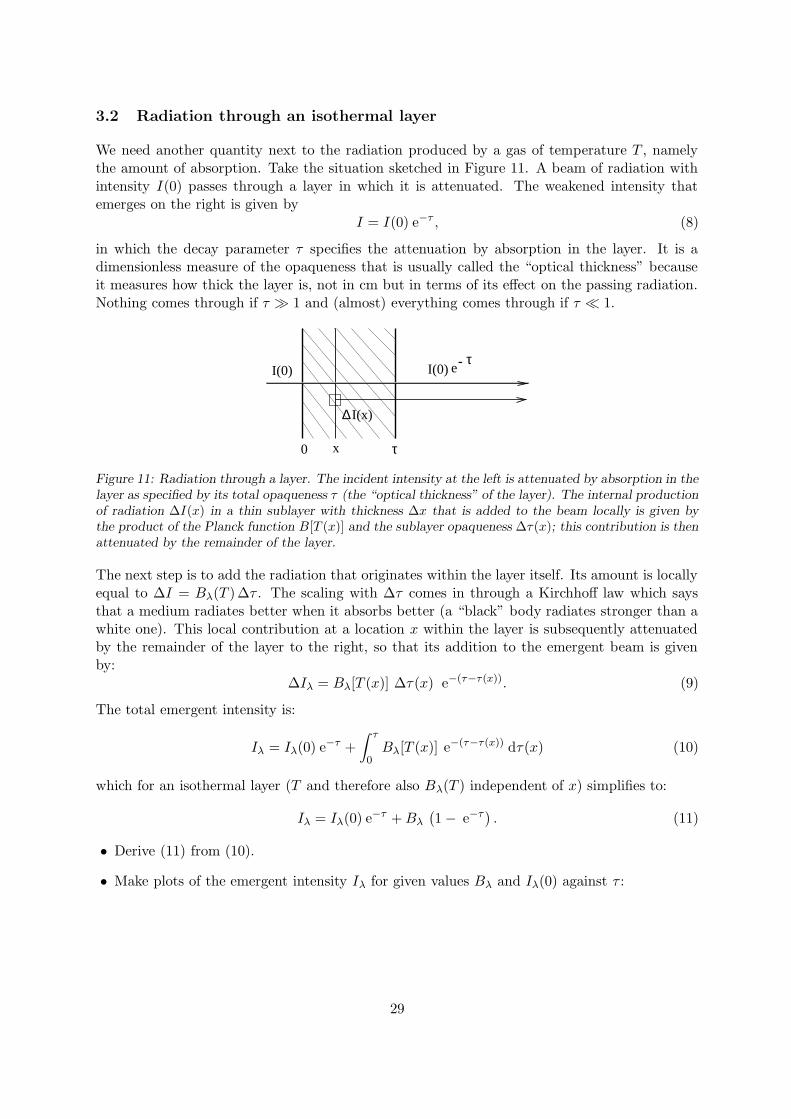
We need another quantity next to the radiation produced by a gas of temperature T , namelythe amount of absorption. Take the situation sketched in Figure 11. A beam of radiation withintensity I(0) passes through a layer in which it is attenuated. The weakened intensity thatemerges on the right is given by

I = I(0) e−τ , (8)

in which the decay parameter τ specifies the attenuation by absorption in the layer. It is adimensionless measure of the opaqueness that is usually called the “optical thickness” becauseit measures how thick the layer is, not in cm but in terms of its effect on the passing radiation.Nothing comes through if τ � 1 and (almost) everything comes through if τ � 1.

I(x)

eτ-

∆

I(0)I(0)

0 τx

Figure 11: Radiation through a layer. The incident intensity at the left is attenuated by absorption in thelayer as specified by its total opaqueness τ (the “optical thickness” of the layer). The internal productionof radiation ∆I(x) in a thin sublayer with thickness ∆x that is added to the beam locally is given bythe product of the Planck function B[T (x)] and the sublayer opaqueness ∆τ(x); this contribution is thenattenuated by the remainder of the layer.

The next step is to add the radiation that originates within the layer itself. Its amount is locallyequal to ∆I = Bλ(T )∆τ . The scaling with ∆τ comes in through a Kirchhoff law which saysthat a medium radiates better when it absorbs better (a “black” body radiates stronger than awhite one). This local contribution at a location x within the layer is subsequently attenuatedby the remainder of the layer to the right, so that its addition to the emergent beam is givenby:

∆Iλ = Bλ[T (x)] ∆τ(x) e−(τ−τ(x)). (9)

The total emergent intensity is:

Iλ = Iλ(0) e−τ +

∫ τ

0Bλ[T (x)] e−(τ−τ(x)) dτ(x) (10)

which for an isothermal layer (T and therefore also Bλ(T ) independent of x) simplifies to:

Iλ = Iλ(0) e−τ + Bλ

(

1 − e−τ )

. (11)

• Derive (11) from (10).

• Make plots of the emergent intensity Iλ for given values Bλ and Iλ(0) against τ :

29

B=2.

tau=indgen(101)/10.+0.01 ; set array tau = 0.01-10 in steps 0.01

int=tau ; declare float array of the same size

for I0=4,0,-1 do begin ; step down from I0=4 to I0=0

for i=0,100 do int(i)=I0 * exp(-tau(i)) + B*(1-exp(-tau(i)))

if i0 eq 4 then plot,tau,int,$

xtitle=’tau’,ytitle=’Intensity’,charsize=1.3

if i0 ne 4 then oplot,tau,int

endfor

• How does Iλ depend on τ for τ � 1 when Iλ(0) = 0 (add ,/xlog,/ylog to study the behaviorat small τ)? And when Iλ(0) > Bλ? Such a layer is called “optically thin”, why?

• A layer is called “optically thick” when it has τ � 1. Why? The emergent intensity becomesindependent of τ for large τ . Can you explain why this is so in physical terms?

3.3 Spectral lines from a solar reversing layer

We will now apply the above result for an isothermal layer to a simple model in which theFraunhofer lines in the solar spectrum are explained by a “reversing layer”. Cecilia Payne hadthis model in mind when she plotted her Saha-Boltzmann population curves. She thought thather curves described the local density of the line-causing atoms and ions within stellar reversinglayers.

surfaceT

λ

Tlayer

τ

Figure 12: The Schuster-Schwarzschild or reversing-layer model. The stellar surface radiates an inten-sity given by Bλ(Tsurface). The shell around the surface only affects this radiation at the wavelengthswhere atoms provide a bound-bound transition between two discrete energy levels. These spectral linetransitions cause attenuation τλ. The layer has temperature Tlayer and gives a thermal contributionBλ(Tlayer) [1 − exp(−τλ)] as in Eq. (11).

Schuster-Schwarzschild model. The basic assumptions are that the continuous radiation,without spectral lines, is emitted by the stellar surface and irradiates a separate layer with theintensity

Iλ(0) = Bλ(Tsurface), (12)

and that this layer sits as a shell around the star and causes attenuation and local emission only

at the wavelengths of spectral lines. Thus, the shell is thought to be made up exclusively byline-causing atoms or ions.

30

The star is optically thick (any star is optically thick!) so that its surface radiates with theτ � 1 solution Iλ = Bλ(Tsurface) of (11), but the shell may be optically thin or thick at theline wavelength depending on the atom concentration. The line-causing atoms in the shell havetemperature Tlayer so that the local production of radiation in the layer at the line wavelengthsis given by Bλ(Tlayer)∆τ(x). The emergent radiation at the line wavelengths is then given by(11) and (12) as:

Iλ = Bλ(Tsurface) e−τλ + Bλ(Tlayer)(

1 − e−τλ)

. (13)

Voigt profile. The opaqueness τ in (13) has gotten an index λ because it varies over thespectral line. When atoms absorb or emit a photon at the energy at which the valence electronmay jump between two bound energy levels (bound electron orbits), the effect is not limitedto an infinitely sharp delta function at λ with hc/λ = χr,s − χr,t but it is a little bit spreadout in wavelength. An obvious cause for such “line broadening” consists of the Doppler shiftsgiven by individual atoms due to their thermal motions. Other broadening is due to Coulombinteractions with neighboring particles. This broadening distribution is described by

τ(u) = τ(0) V (a, u) (14)

where V is called the Voigt function and u measures the wavelength separation ∆λ = λ − λ(0)from the center of the line at λ = λ(0) in dimensionless units

u ≡ ∆λ/∆λD, (15)

where ∆λD is the “Doppler width” defined as

∆λD ≡ λ

c

√

2kT/m (16)

with m the mass of the line-causing particles (for example iron with mFe ≈ 56mH ≈ 9.3 ×10−23 g). The parameter a in (14) measures the amount of Coulomb disturbances (called“damping”). Stellar atmospheres typically have a ≈ 0.01 − 0.5. The Voigt function V (a, u)is defined as:

V (a, u) ≡ 1

∆λD√

π

a

π

∫ +∞

−∞

e−y2

(u − y)2 + a2dy. (17)

It represents the convolution (smearing) of a Gauss profile with a Lorentz profile and thereforehas a Gaussian shape close to line center (u = 0) due to the thermal Doppler shifts (“Dopplercore”) and extended Lorentzian wings due to disturbances by other particles (“damping wings”).A reasonable approximation is obtained by taking the sum rather than the convolution of thetwo profiles:

V (a, u) ≈ 1

∆λD√

π

[

e−u2

+a√π u2

]

. (18)

• Start the IDL Online Help by typing ? on the command line. Inspect the description ofthe VOIGT(a,u) function. We might have programmed approximation (18), but since IDLfurnishes the real thing we will use that instead.

• Plot the Voigt function against u from u = −10 to u = +10 for a = 0.1:

u=indgen(201)/10.-10. ; u = -10 to 10 in 0.1 steps

vau=u ; declare same-size array

a=0.1 ; damping parameter

for i=0,200 do vau(i)=VOIGT(a,abs(u(i))) ; taking abs corrects IDL errors

plot,u,vau,yrange=[0,1] ; yrange fixed to compare plots

31

• Cursor back up and vary the value of a between a = 1 and a = 0.001 to see the effect of thisparameter. Also add ,/ylog (without setting yrange) to inspect the far wings of the profile.Use approximation (18) to explain what you see.

Emergent line profiles. You are now able to compute and plot stellar spectral line profilesby combining (13) with (14). Again use the dimensionless u units for the wavelength scale sothat you don’t have to evaluate the Doppler width ∆λD.

• Write an IDL sequence that computes Schuster-Schwarzschild line profiles. Take Tsurface =5700 K, Tlayer = 4200 K, a = 0.1, λ = 5000 A. These values are good choices for the solarphotosphere as seen in the optical part of the spectrum. First plot a profile I against u forτ(0) = 1:

Ts=5700 ; solar surface temperature

Tl=4200 ; solar T-min temperature = ‘reversing layer’

a=0.1 ; damping parameter

wav=5000.D-8 ; wavelength in cm

tau0=1 ; reversing layer thickness at line center

u=indgen(201)/10.-10. ; u = -10 to 10 in 0.1 steps

int=u ; declare array

for i=0,200 do begin

tau=tau0 * VOIGT(a,abs(u(i)))

int(i)=PLANCK(Ts,wav) * exp(-tau) + PLANCK(Tl,wav)*(1.-exp(-tau))

endfor

plot,u,int

• Study the appearance of the line in the spectrum as a function of τ(0) over the range log τ(0) =−2 to log τ(0) = 2. Example:

tau0=[0.01, 0.05, 0.1, 0.5, 1, 5, 10, 50, 100]

for itau=0,8 do begin

for i=0,200 do begin

tau=tau0(itau) * VOIGT(a,abs(u(i)))

int(i)=PLANCK(Ts,wav) * exp(-tau) + PLANCK(Tl,wav)*(1.-exp(-tau))

endfor

oplot,u,int

endfor

• How do you explain the profile shapes for τ(0) � 1?

• Why is there a low-intensity saturation limit for τ � 1?

• Why do the line wings develop only for very large τ(0)?

• Where do the wings end?

• For which values of τ(0) is the layer optically thin, respectively optically thick, at line center?And at u = 5?

• Now study the dependence of these line profiles on wavelength by repeating the above forλ = 2000 A (ultraviolet) and λ = 10 000 A (near infrared). What sets the top value Icont

32

and the limit value reached at line center by I(0)? Check these values by computing themdirectly on the command line. What happens to these values at other wavelengths?

• Observed spectra that are measured in detector counts without absolute intensity calibration(as in your Clea-Spec data gathering in Exercise 1) are usually scaled to the local continuumintensity by plotting Iλ/Icont against wavelength. Do that for the above profiles at the samethree wavelengths:

for iwav=1,3 do begin

wav=(iwav^2+1)*1.D-5 ; wav = 2000, 5000, 10000 Angstrom

for itau=0,8 do begin

for i=0,200 do begin

tau=tau0(itau) * VOIGT(a,abs(u(i)))

int(i)=PLANCK(Ts,wav) * exp(-tau) + PLANCK(Tl,wav)*(1.-exp(-tau))

endfor

int=int/int(0) ; convert into relative intensity

if iwav eq 1 and itau eq 0 then plot,u,int

if iwav eq 1 and itau gt 0 then oplot,u,int

if iwav eq 2 then oplot,u,int,linestyle=1 ; dotted

if iwav eq 3 then oplot,u,int,linestyle=4 ; dash dot dot dot

endfor

endfor

• Explain the wavelength dependences in this plot.

3.4 The equivalent width of spectral lines

Your profile plots demonstrate that the growth of the absorption feature in the spectrum forincreasing τ(0) is faster for small τ(0) then when it “saturates” for larger τ(0). Minnaert andcoworkers introduced the equivalent width Wλ as a line-strength parameter to measure thisgrowth quantitively. It measures the integrated line depression in the normalized spectrum:

Wλ ≡∫

Icont − I(λ)

Icontdλ (19)

so that its value is the same as the width of a rectangular piece of spectrum that blocks thesame amount of spectrum completely (Figure 13). We will express it here in the dimensionlesswavelength units u.

• In order to add such profile integration it becomes handy to turn the profile computationinto an IDL function PROFILE(a,tau0,u):

33

Wλ

0λ

Iλ

Figure 13: The equivalent width of a spectral line is the width of a rectangular piece of fully blockedspectrum with the same spectral area as the integrated line depression.

function profile,a,tau0,u

; return a Schuster-Schwarzschild profile

; input: a = damping parameter

; tau0 = SS layer thickness at line center

; u = wavelength array in Doppler units

; output: int = intensity array

Ts=5700

Tl=4200

wav=5000.E-8

int=u

usize=SIZE(u) ; IDL SIZE returns array type and dimensions

for i=0,usize(1)-1 do begin

tau=tau0 * VOIGT(a,abs(u(i)))

int(i)=PLANCK(Ts,wav)*exp(-tau) + PLANCK(Tl,wav)*(1.-exp(-tau))

endfor

return,int

end

• Check your routine:

u=indgen(1001)/2.5-200. ; u = -200 to +200 in steps of 0.4

a=0.1

tau0=1e2

int=profile(a,tau0,u)

plot,u,int

• Continue by computing the equivalent width with the IDL TOTAL function (check it out inthe Online Help):

reldepth=(int(0)-int)/int(0) ; line depth in relative units

plot,u,reldepth

eqw=total(reldepth)*0.4 ; integral = TOTAL times interval

print,eqw

The wide range of u specified above is needed to fully accommodate the extended line wingsthat develop at large τ(0), otherwise int(0) will not equal Icont. However, the sampling shouldbe finely spaced around line center to get the proper summation for narrow lines at small τ(0).

34

Spectral line codes therefore often use equidistant wavelength spacing over the Doppler core butlogarithmic wavelength spacing in the damping wings.

Figure 14: Empirical curve of growth for solar Fe I and Ti I lines. Taken from Mihalas (1970) who tookit from Wright (1948). Wright measured the equivalent widths of 700 lines in the Utrecht Atlas. Thequantity Xf along the x axis scales with the product of the transition probability and the populationdensity of the lower level of each line. The populations were computed from the Saha-Boltzmann laws asin Exercise 2. The transition probabilities were measured in the laboratory. The normalization of W byλ removes the λ-dependence of the Doppler width defined by (16).

3.5 The curve of growth

The idea behind the equivalent width was obviously that the amount of spectral blocking shouldbe a direct measure of the number of atoms in the reversing layer. They should set the opaquenessτ(0) of the layer. Your profile plots illustrate that the profile growth is only linear with τ(0) forτ(0) � 1. The “curve of growth” describes the full dependence: the growth of the line strengthwith the line-causing particle density. Figure 14 shows an observed example.

• Compute and plot a curve of growth by plotting log Wλ against log τ(0):

tau0=10^(indgen(61)/10.-2.) ; 10^-2 to 10^4, 0.1 steps in the log

eqw=tau0 ; same size array

for i=0,60 do begin

int=profile(a,tau0(i),u)

reldepth=(int(0)-int)/int(0)

eqw(i)=total(reldepth)*0.4

endfor

plot,tau0,eqw,xtitle=’tau0’,ytitle=’equivalent width’,/xlog,/ylog

35

• Explain what happens in the three different parts.

• The first part has slope 1:1, the third part has slope 1:2 in this log-log plot. Why?

• Which parameter controls the location of the onset of the third part? Give a rough estimateof its value for solar iron lines through comparison with Figure 14.

• Final question: of which parameter should you raise the numerical value in order to produceemission lines instead of absorption lines? Change it accordingly and rerun your programsto produce emission profiles and an emission-line curve of growth. Avoid plotting negativeWλ values logarithmically by:

plot,tau0,abs(eqw),$

xtitle=’tau0’,ytitle=’abs(equivalent width)’,/xlog,/ylog

36

Epilogue

In these three exercises “Stellar Spectra A” you have quickly gone through half a century ofstellar spectroscopy (the first half of the twentieth century), ending with a model of spectral lineformation that roughly explains the strengths and shapes of solar line profiles. Combination ofthis model with Saha-Boltzmann routines as in Exercise 2 explains stellar spectra throughoutthe Hertzsprung-Russell diagram. However, the model is very simple. Its two major deficienciesare:

– use of the single-layer Schuster-Schwarschild description (Exercise 3).It is obviously unrealistic to stick all line-causing particles together in a separate layer. Thegas in a stellar atmosphere is well mixed; the gas particles contribute to local absorptionand emission with continuum-causing processes and line-causing processes at the same time.A much better description is therefore to have say a hundred layers instead of a single one,each with its own τ c(i) for the continuum and additional τ l(i) for the spectral line. If thetemperature T (i) is then set to smoothly decline outwards, a fairly realistic model of a stellaratmosphere results.

Setting the ratio τ l/τ c constant for all i would make this many-layer model a “Milne-Eddington” atmosphere, a much better description than the Schuster-Schwarzschild one.

Computing τ c(i) and τ l(i) in detail from the Saha-Boltzmann laws would make it an “LTEmodel atmosphere”, where the “Local” in LTE = Local Thermodynamic Equilibrium alludesto using the local temperature within a stratified atmosphere in the TE laws. Such local-equilibrium modeling has been used for stellar abundance determination throughout thesecond half of the twentieth century. It is treated in exercises “Stellar Spectra B: LTE lineformation”.

– use of the TE partitioning laws (Exercises 2 and 3).We have assumed that the temperature defines both the particle populations (Saha andBoltzmann laws; Exercise 2) and the production of radiation (Planck law; Exercise 3). TheseTE laws are accurate in the stellar interior and hold reasonably well in the deeper parts of astellar atmosphere, but not in the outer parts. For example, they do not hold at all in thesolar corona. Its high temperature (Te ≈ 2 × 106 K) and low density (Ne ≈ 106 cm−3) causeionization to very high stages but without reaching thermodynamical equilibrium becausethe X-ray radiation from the ions escapes directly from the corona and represents a limitingenergy loss. As a result, the production of coronal radiation falls very far below the coronalPlanck function, and the ion populations are far below the Saha prediction.

The TE laws hold much better for the stellar photospheres from which the visible radiationescapes. Although that radiation leak contributes most of the total stellar energy loss, itrepresents only a tiny loss in comparison to the local photospheric thermal energy content.LTE is therefore a reasonable assumption for many photospheric lines and continua — but byno means for all and certainly not for chromospheric lines such as Ca+K and Hα in the solarspectrum. Exercises “Stellar Spectra C: NLTE line formation” treat techniques appropriateto those.

37

References

Abt, H. A., Meinel, A. B., Morgan, W. W., and Tapscott, J. W.: 1968, An Atlas of Low-

Dispersion Grating Stellar Spectra, Kitt Peak National Observatory, Tucson, USA

Allen, C. W.: 1976, Astrophysical Quantities, Athlone Press, Univ. London

De Jager, C., Schadee, A., Svestka, Z., Van Tend, W., Machado, M. E., Strong, K. T., andWoodgate, B. E.: 1983, Solar Phys. 84, 205

Hearnshaw, J. B.: 1986, The analysis of starlight. One hundred and fifty years of astronomical

spectroscopy , Cambridge Univ. Press, Cambridge UK

Kurucz, R. L., Furenlid, I., Brault, J. W., and Testerman, L.: 1984, Solar Flux Atlas from 296

to 1300 nm, NSO Atlas Nr. 1, National Solar Observatory, Sunspot, New Mexico

Mihalas, D.: 1970, Stellar Atmospheres, W. H. Freeman and Co., San Francisco (first edition)

Minnaert, M. G. J., Mulders, G. F. W., and Houtgast, J.: 1940, Photometric Atlas of the Solar

Spectrum 3332 A to 8771 A, Schnabel, Amsterdam

Moore, C. E., Minnaert, M. G. J., and Houtgast, J.: 1966, The Solar Spectrum 2935 A to

8770 A. Second Revision of Rowland’s Preliminary Table of Solar Spectrum Wavelengths,NBS Monograph 61, National Bureau of Standards, Washington

Novotny, E.: 1973, Introduction to stellar atmospheres and interiors, Oxford Univ. Press, NewYork

Payne, C. H.: 1924, Harvard Circular 256, 1

Payne, C. H.: 1925, Stellar Atmospheres, Harvard Observatory Monographs No. 1, Cambridge,Mass.

Rybicki, G. B. and Lightman, A. P.: 1979, Radiative Processes in Astrophysics, John Wiley &Sons, Inc., New York

Schadee, A.: 1964, The Formation of Molecular Lines in the Solar Spectrum, PhD Thesis,Utrecht University

Schadee, A.: 1978, J. Quant. Spectrosc. Radiat. Transfer 19, 517

Wright, K. O.: 1948, Pub. Dominion Astrophys. Obs. 8, 1

38

Brief IDL manual

Why IDL?

--------

IDL is much used in astronomical image processing.

It is an interactive computer language with the following advantages:

- programming language, not a package: make up your own stuff;

- interactive: test out new tricks by trying them statement by statement;

- array notation: a = a + (b < 0) works for whole multi-dimensional arrays.

The disadvantage is that IDL licenses are very expensive. The Student

License is cheaper but limited to array size 65536 (256x256 pixel images).

Manuals

-------

The online help is good.

There are also complete IDL User’s Guides in book form (3-4 big volumes).

The student version manual ("Learning IDL") is compact but fairly good.

The IDL astronomy library sits at

http://idlastro.gsfc.nasa.gov/homepage.html

Solar IDL software is found at:

http://www.lmsal.com/ssw

IDL as interpreter

------------------

IDL works directly on the command line when you hit return.

This makes it easy to try new statements and statement sequences.

The up cursor arrow brings back earlier commands.

Try out the following IDL statements on the command line:

; on-line help

? ; inspect some IDL routines

; number games

print,3*5 ; semicolon = comment (IDL skips rest of line)

a=3*5

help,a ; show nature and value of this variable

help,A ; IDL is case-insensitive

d=32767 ; integers run from -32768 to + 32768

print,d+1 ; so what happens here?

print,d+1.

print,3/5

print,3/5. ; one floating number makes the result a float

a=[1,2,3,4,5,6] ; IDL variables can be (multi-dimensional) arrays

a=[a,7] ; lengthen array A by adding value at its end

print, a, 1E6*a ; single precision: 6 significant digits, <10^38

print, a, 1D6*a ; double precision: 16 significant digits

print, a, 1/a

39

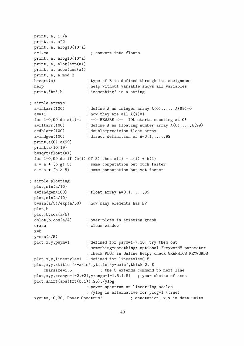
print, a, 1./a

print, a, a^2

print, a, alog10(10^a)

a=1.*a ; convert into floats

print, a, alog10(10^a)

print, a, alog(exp(a))

print, a, acos(cos(a))

print, a, a mod 2

b=sqrt(a) ; type of B is defined through its assignment

help ; help without variable shows all variables

print,’b=’,b ; ’something’ is a string

; simple arrays

a=intarr(100) ; define A as integer array A(0),....,A(99)=0

a=a+1 ; now they are all A(i)=1

for i=0,99 do a(i)=i ; ==> BEWARE <== IDL starts counting at 0!

a=fltarr(100) ; define A as floating number array A(0),...,A(99)

a=dblarr(100) ; double-precision float array

a=indgen(100) ; direct definition of A=0,1,....,99

print,a(0),a(99)

print,a(10:19)

b=sqrt(float(a))

for i=0,99 do if (b(i) GT 5) then a(i) = a(i) + b(i)

a = a + (b gt 5) ; same computation but much faster

a = a + (b > 5) ; same computation but yet faster

; simple plotting

plot,sin(a/10)

a=findgen(100) ; float array A=0,1,....,99

plot,sin(a/10)

b=sin(a/5)/exp(a/50) ; how many elements has B?

plot,b

plot,b,cos(a/5)

oplot,b,cos(a/4) ; over-plots in existing graph

erase ; clean window

x=b

y=cos(a/5)

plot,x,y,psym=1 ; defined for psym=1-7,10; try them out

; something=something: optional "keyword" parameter

; check PLOT in Online Help; check GRAPHICS KEYWORDS

plot,x,y,linestyle=1 ; defined for linestyle=0-5

plot,x,y,xtitle=’x-axis’,ytitle=’y-axis’,thick=2, $

charsize=1.5 ; the $ extends command to next line

plot,x,y,xrange=[-2,+2],yrange=[-1.5,1.5] ; your choice of axes

plot,shift(abs(fft(b,1)),25),/ylog

; power spectrum on linear-log scales

; /ylog is alternative for ylog=1 (true)

xyouts,10,30,’Power Spectrum’ ; annotation, x,y in data units

40

xyouts,.75,.75,’Power Spectrum’,/normal ; annotation, axis-length units

; more displays

z=b#a ; z(i,j)=b(i)*a(j); full matrix multiplication: ##

help,z ; so this is a 2-dim (100,100) float array

print,z[0:5,0:5] ; both square brackets and parentheses permitted

plot,indgen(50),z[2,*] ; plot 3rd column of array z

plot,indgen(50),z(*,49) ; plot bottom row of array z

contour,z ; just for fun

surface,z ; just for fun

shade_surf,z ; just for fun - but only in a small window

window,1,xsize=200,ysize=200 ; open small window, size in pixels

shade_surf,z

wdelete,1 ; delete window 1

show3,z ; just for fun

; PostScript output

set_plot,’ps’ ; now write to PostScript file instead of window

device,filename=’surface_1.ps’ ; choose filename

show3,z ; all IDL output commands now write to that file

device,/close ; done

set_plot,’win’ ; back to output on Windows95 screen

set_plot,’x’ ; idem for Unix

help,/device ; ,/device is the same as using ,device=1 (enable)

; image display

tv,z ; show array as image

zsize=SIZE(z) ; get array type and size

nx=2*zsize(1)

ny=2*zsize(2) ; etcetera for more dimensions; zsize(0)=type

z=rebin(z,nx,ny) ; resample z to make its display bigger

wdelete

window,xsize=nx,ysize=ny ; window equal to image size

z8=bytscl(z) ; scales dynamic range to 8 bits (shades 0 - 255)

print,min(z),max(z),min(z8),max(z8) ; list extrema

tv,z8 ; display image with maximum contrast on screen

tvscl,z ; same as tv,bytescl(z)

profiles,z ; measurent tool for showing image values

; stop it with right mouse button (cursor on image)

loadct ; set colour table

adjct ; tool to adjust greyscale table

xpalette ; tool to adjust color table

xloadct ; idem

tvscl,z8>127 ; display only the brighter half of the pixels

erase

tvscl,z(0:nx/2,0:ny/2) ; bottom-left quarter of the image

wdelete

tvscl,congrid(z,188,188,/interp) ; arbitrary resizing with interpolation

41

; read/write files

openw,1,’myfile.ext’ ; open file myfile.ext on logical unit 1 for writing

printf,1,z ; write free-format file

close,1 ; free lun 1

openr,1,’myfile.ext’ ; now open that file for reading

zz=z ; define variable type and size

readf,1,zz ; read free-format file

close,1

(use: - WRITEU, READU to write/read large files unformatted = faster;

- image=assoc(lun,bytarr(nx,ny)) to get single images from a movie)

; saving IDL command sequences

journal,’filename’ ; copies all typed commands to a file

@filename ; executes a sequence of IDL commands in a file

save,filename=’name.sav’ ; saves a full session (not in Student Version)

restore,’name.sav’ ; restores a session save set

Procedures and functions

------------------------

Start a new file pract.idl or procedurename.pro or functionname.pro;

edit it (Windows: IDL desktop; Unix: external editor or idlde).

PRO procedurename, param1, param2

; this one does this...

; parameters: param1 = etc ; input value or input/output parameter

IDL statements

IDL statements

END

FUNCTION functionname, param1, param2, param3, ....

; this one does this...

; parameters: param1 =etc ; input value or input/output parameter

IDL statements

IDL statements

something=...

RETURN,something

END

IDL statement ; start of main-level program

IDL statement

STOP ; for command-line inspections, continue with .CON

IDL statement

END

A sequence of IDL statements after the last procedure or function

that does not start with PRO or FUNCTION makes up the main level

42

program. It should end with END. You run it with .R FILENAME.

After program completion all variables are available for inspection

on the command line. Use this main level for trying out new things.

When such a sequence is complete, then turn it into a procedure or

function. The latter may go to a separate NAME.PRO file or may remain

in your main FILENAME.IDL file, above the statement part.

Using procedures and functions

------------------------------

IDL> .run procedurename ; compilation (only main program is run)

IDL> procedurename,param1,... ; run compiled procedure

IDL> .rnew procedurename ; first discards all existing variables

IDL> .com functionname.pro ; compilation

IDL> a=functionname(param1,...) ; evaluate compiled function

example (in a separate file ADDUP.PRO):

function addup,arr

; sums linear array ARR - but IDL TOTAL is faster and more general!

arraysize=SIZE(arr)

if (arraysize(0) ne 1) then print,’addup input is not a 1D array’

sumarr=0

for i=0,arraysize(1)-1 do sumarr=sumarr+arr(i)

return,sumarr

end

IDL> .run addup ; recompile after every program change

IDL> try=findgen(100) ; floats 0.,......,99.

IDL> print,addup(try)

IDL> print,total(try) ; check with IDL array summation

"Disappearing variables": after an error in a procedure or function your

session stops within that procedure/function. HELP displays only the

local variables. RETURN gets you one level higher; RETALL gets you

back to the top level.

STOP in a procedure/function/main stops it there to let you inspect the

local variables at that place in the statement sequence.

Continue with .continue (or .con).

Program structures

------------------

if i>16 then begin

IDL statement

IDL statement

endif else begin

IDL statement

IDL statement

43

endelse

if ( y eq 3) then x=2 else x=1 ; relational operators: EQ NE LE LT GE GT

for j=0,9 do number(j)=sin(region[j] * !pi) ; ! gets system variable

for j=0,20,2 do begin

number[j] = sin(region[j] * !pi)

region[j]=0

endfor

while (a and (cnt ne 0)) do begin ; logical operators: AND OR XOR

print, ’Still going at count: ’, cnt

cnt=cnt-1

endwhile

if n eq 0 goto, finish

IDL statement

IDL statement

finish:

return

; but since good programmers don’t use goto’s, a better solution is:

if n neq 0 then begin

IDL statement

IDL statement

endif

return

Programming style hints

-----------------------

- don’t forget that IDL array indices start at 0

- split programs in separate procedures and functions

- use parameters instead of numbers to get dynamical adaptivity

- use SIZE(array) to get array dimensions for general procedures

- choose clear variable names

- add lots of comments (in English please)

- add detailed explanation at procedure/subroutine start

(some libraries do this between ;+ and ;- lines and cut out these

comment blocks for automatic manual generation)

- answer a routine call without parameters or () with a specification:

IF N_PARAMS(0) LT 1 THEN BEGIN

PRINT,’procedure xxxx requires parameters: yyy, zzz’

RETURN

ENDIF

- indent BEGIN ... END structures

- use capitals for IDL terms, routines and operators

- use capitals for image arrays in image processing

- JOURNAL,’filename’ records all your command-line entries, useful for

44

subsequent conversion into programs.

45

Brief LaTeX manual

Template

========

Begin your writing by copying the template file

http://www.astro.uu.nl/~rutten/ssa/latex-template.tex

to your work directory as "report.tex".

Run it to see what it does.

(I have many more LaTeX template files available at

http://www.astro.uu.nl/~rutten/ under "LaTeX and BibTeX stuff").

I more extensive manual (not much shorter than Lamport’s own

LaTeX book which I prefer to use myself) is found at

ftp://ftp.tex.ac.uk/tex-archive/info/lshort/english/lshort.pdf

LaTeX writing tips

==================

- type text as you are used to. Pure ASCII! Good habits:

- start each sentence on a new line, makes for easier changing

- indent equations and environments as you do in programming

- add comments to clarify your layout and what you are doing

(LaTeX skips the remainder of a line after %, type \% to get %.)

- use hard returns to maintain this layout.

- new paragraph = 1 or more blank lines, not ....\\[1ex]

- spaces:

multiple spaces is same as single space

no-line-break-space: ~ R.J.~Rutten, 1083.0~nm line

(otherwise you may get the unit nm on the next line)

code space after period after small character: Dr.\ C. Zwaan

(otherwise LaTeX adds more space taking it to be end of sentence)

code space after LaTeX command: 4554~\AA\ line, but \AA. Nordlund

(otherwise LaTeX eats up the space as command delimiter)

- dashes: hyphen = - magneto-acoustic

longer dash = -- 5--min oscillation

longest dash = --- 399.3---399.6~nm wavelength region

he said---but I think otherwise

- quotation marks: use ‘‘......’’, not "...."

- mathematics:

$...$ for in-text math

never use \frac in in-text math (too small), only use $a/b$

\begin{equation}

........ for displayed & numbered equation (indent!)

\label{eq:whatever}

46

\end{equation}

Use \sin, \cos, \exp etc ($sin$ means product s i n)

Use roman alphabet for non-mathematical indices

(code only math variables in math notation ($x$), cf. A&A manual):

$T_{\rm eff}$

($T_{eff}$ makes eff = product e, f and f)

\begin{equation}

B_\nu(T) = \frac{2\pi m_{\rm e} c^2}{h^3}

%% e = electron

\frac{1}{\exp{-h\nu/kT}-1}

\label{eq:Planck}

\end{equation}

(rrmacros.tex defines full \rm alphabets as \rma, \rmA etc)

Use {\rm d} or \partial for differential d

Add space with \, before differential d, {\rm e}^{..} etc

Add punctuation after equations, just as in normal text

- numbers and units:

$B_\nu = 5\,10^12$~erg\,cm$^{-2}$s$^{-1}$sterad$^{-1}$

$v=50$~km\,s$^{-1}$ velocity

180~s 10~mHz

a $40 \times 30$~arcsec$^2$ field

alternative is to use smaller blank space with \,:

50\,km\,s$^{-1}$ velocity

the Ba\,II\,4554\,\AA\ line (NB: \ after \AA for normal space)

10\,mHz frequency

for $\lambda \approx 160$\,nm one sees

- crossreferences:

keep all references to figures, tables, equations, sections

dynamic by adding labels to them:

\label{fig:power images}

\label{tab:lines}

\label{eq:mass conservation}

\label{sec:discuss}

and refering to these as:

in Sect.~\ref{sec:discuss} we discuss

Figure~\ref{fig:power images} shows power spectra

(see Figs.~\ref{fig:xx}, \ref{fig:xx}---\ref{fig:xx})

inserting this result into eq.~(\ref{eq:mass conservation})

use Figure in full at the start of a sentence, Fig.~ elsewhere.

NB: LaTeX needs to be run twice to get all crossreferences right.

- literature citations and references:

Most astronomers and astronomy journals use the name-year system:

.... by Rutten and Schrijver (1994)

(see Schrijver, 1993e; Rutten, 1993).

.... (cf. Rutten & Schrijver 1994)

47

Exceptions are Nature and ESA proceedings (numbered references)

These are all generated automatically by BibTeX. A manual that

explains my way of using BibTeX together with ADS is available at

http://www.astro.uu.nl/~rutten/

under the heading Macros, styles, templates, etc.

Appropriate style files and templates are found there also.

Processing problems

===================

LaTeX errors are usually due to unmatched pairs of $$, {}, \begin &

\end. (I also tend to often mistype $ for & within tables.)

If you don’t like the layout, do NOT try local solutions such as

adding ad-hoc white space, but adapt the formats by more general

commands at the start of your file. You may feel that LaTeX confines

you to overly restrictive straightjackets. Then use TeX commands -

but ask yourself first whether you want to be a professional

typesetter or a professional astronomer. For astronomical papers you

need to confirm strictly to the style of the publisher (e.g. A&A

habits). They have chosen LaTeX in order to fix the layout their way

without bothering you or being bothered by you.

Running LaTeX under Unix

========================

- When your XXXX.tex file is done (or half done), inspect the output.

In Unix or Linux this is done most basically by:

latex XXXX no extension needed for XXXX.tex

xdvi XXXX & this is the previewer; check and edit XXXX.TEX.

When you rerun LateX, the previewer refreshes when

you click on its window top.

You may choose to see the figure inserts or not.

latex XXXX Repeat as needed.

but their are elaborate LaTeX processing shells, also in EMACS.

- When you are happy with what the previewer shows:

ispell XXXXX.tex to check for typos

"man ispell" tells you what to do

(just use a and i)

latex XXXX to produce the final version

- To print the final version (no reason to print any earlier version!):

dvips XXXX -o XXXX.ps

psprint -Pps -i3 XXXX.ps single side printing

psprint -Pps -i1 XXXX.ps double side printing

- Save disk space when you have large postscript figure files with:

48

pscompress *.eps

This lets latex process compressed files too, no need to uncompress

them for use as LaTeX inserts. You can use the filename without .eps

or .eps.Z or eps.gz extension).

- Clean your working directory from all the LaTeX auxiliary files

with a command like:

alias rmtex ’rm *.aux *.dvi *.lis *.log *.blg *.bbl *.toc’

so that it doesn’t clogger up. The XXXX.tex file and the figure ps

files are the only ones you need to keep when you are done, since it

regenerates all the others. I usually keep my postscript figure files

YYYY.ps.Z and YYYY.ps.bb in a subdir \figs per paper.

Figures

=======

- PostScipt figures: use package graphicx for figure inserts.

- always keep your figures small but make their labeling large. In

full-page manuscripts such as conference proceedings it is often

best to combine figures horizontally with a single caption. In A&A

manuscripts or other column-style publications, aim at vertical

panel stacking.

- color figures: don’t ever. Much to expensive for publication.

- images: usually better to cut them down to smaller size first.

- figure location: you have to find by trial where to stick a

particular {figure} environment in your LaTeX input file to make

it appear in a suitable place. It always comes at or after the

place where you put in your text, never before.

49