2007 ICSPC International Conference on SignalProcessing and Communications

TA-P1: Image and Video Processing 6

STEERABLE FILTERS GENERATED WITH THE HYPERCOMPLEX DUAL-TREEWAVELET TRANSFORM

J. Wedekind, B. Amavasai, K. Duttona

Tuesday, November 27th 2007

Microsystems and Machine Vision LaboratoryMaterials Engineering Research Institute

Sheffield Hallam UniversitySheffield

United Kingdom

aThis project was supported by the Nanorobotics EPSRC Basic Technology grant GR/S85696/01

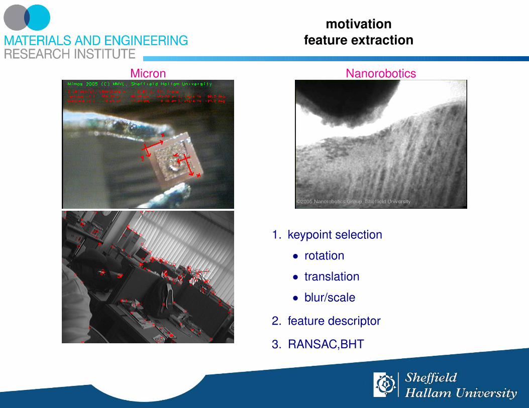
motivationfeature extraction

Micron Nanorobotics

1. keypoint selection

• rotation

• translation

• blur/scale

2. feature descriptor

3. RANSAC,BHT

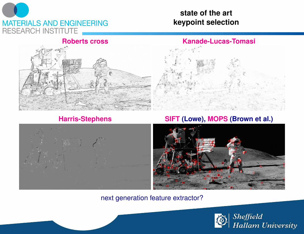
state of the artkeypoint selection

Roberts cross

Harris-Stephens

Kanade-Lucas-Tomasi

SIFT (Lowe), MOPS (Brown et al.)

next generation feature extractor?

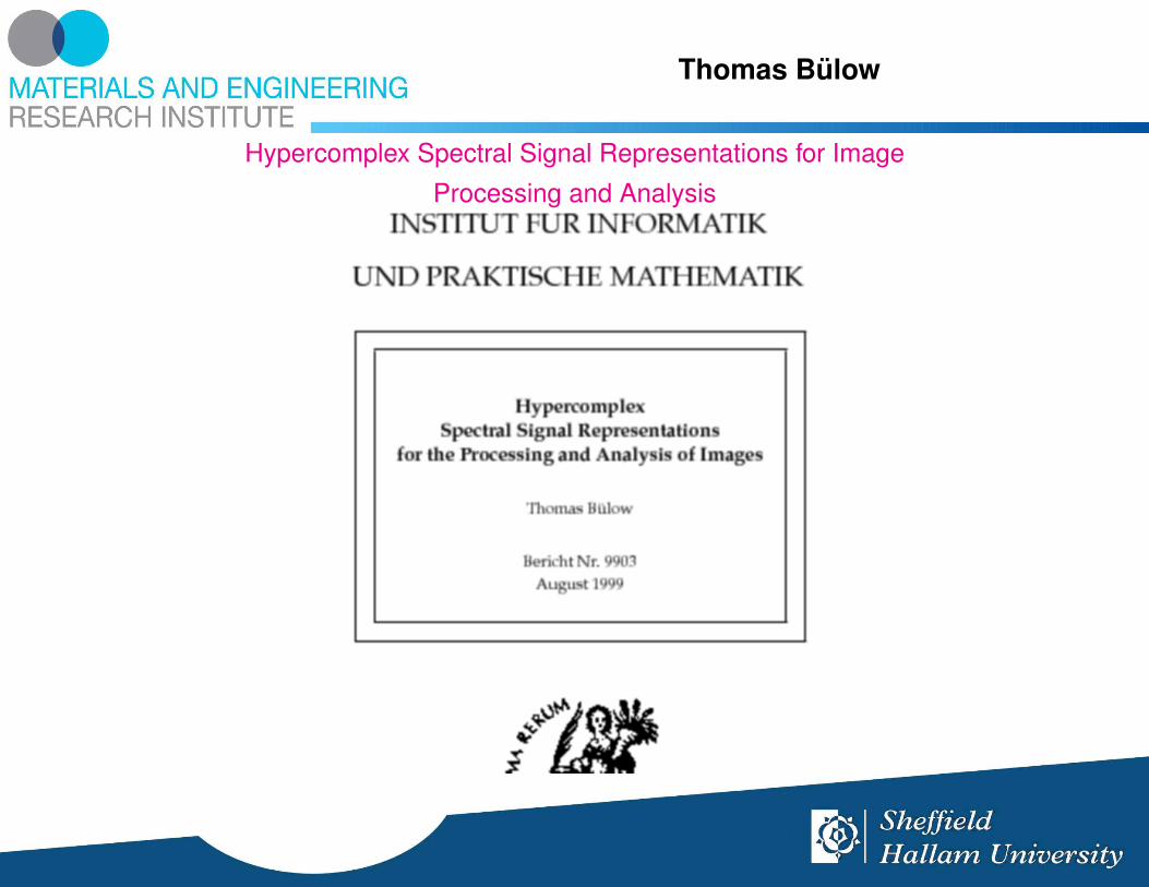
Thomas Bulow

Hypercomplex Spectral Signal Representations for ImageProcessing and Analysis

Ivan Selesnick

The design of approximate Hilbert transform pairs ofwavelet bases

Nick Kingsbury

Image processing with complex wavelets

Ivan Selesnick, Richard G. Baraniuk, Nick Kingsbury

The dual-tree complex wavelet transform

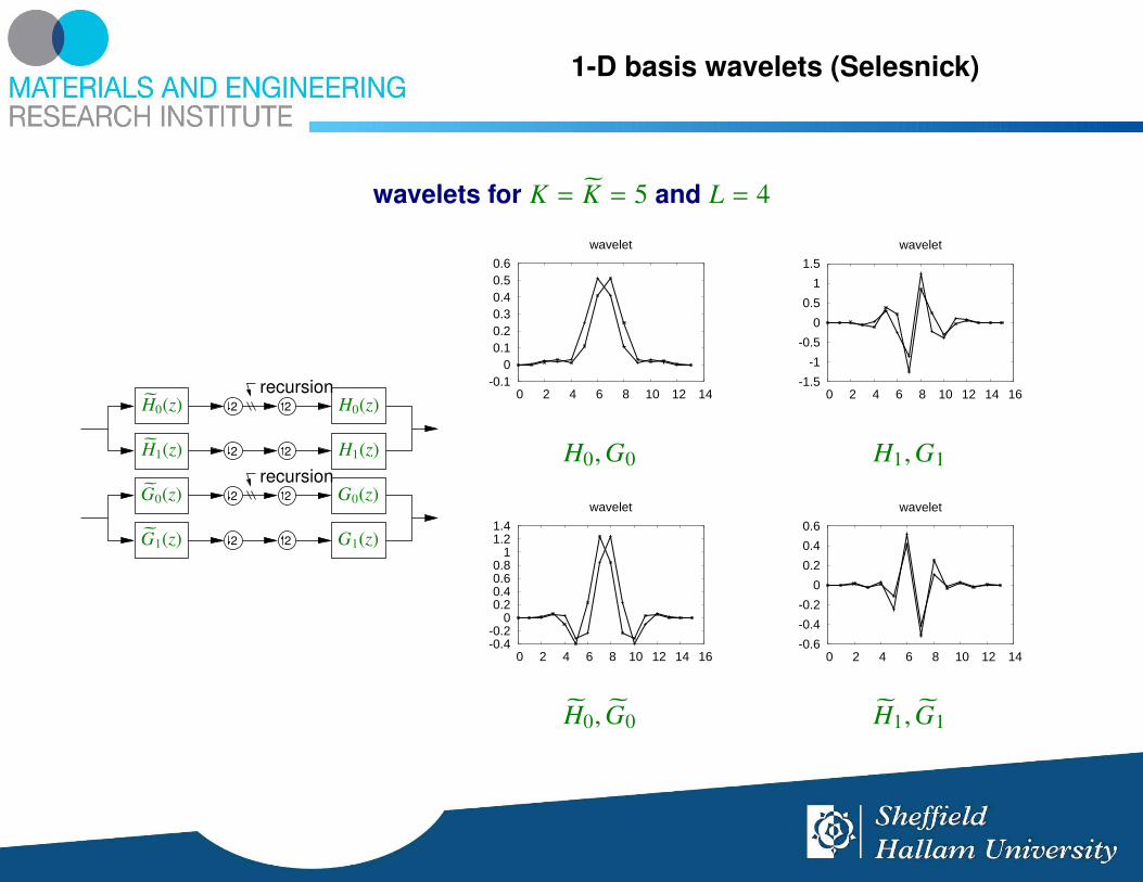
1-D basis wavelets (Selesnick)

wavelets for K = K = 5 and L = 4

recursionG0(z)

G1(z)

2 2G0(z)

G1(z) 2 2

recursion2 2H0(z)

H1(z) 2 2

H0(z)

H1(z)

-0.1 0

0.1 0.2 0.3 0.4 0.5 0.6

0 2 4 6 8 10 12 14

wavelet

H0,G0

-1.5

-1

-0.5

0

0.5

1

1.5

0 2 4 6 8 10 12 14 16

wavelet

H1,G1

-0.4-0.2

0 0.2 0.4 0.6 0.8

1 1.2 1.4

0 2 4 6 8 10 12 14 16

wavelet

H0, G0

-0.6

-0.4

-0.2

0

0.2

0.4

0.6

0 2 4 6 8 10 12 14

wavelet

H1, G1

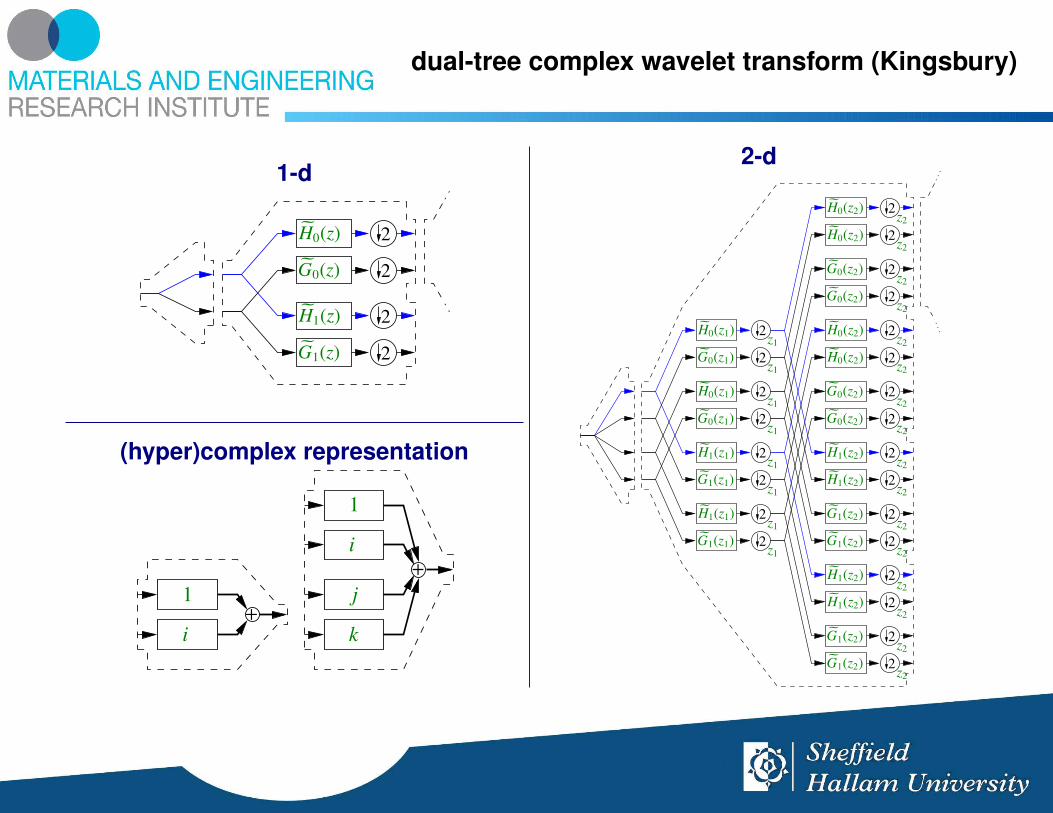
dual-tree complex wavelet transform (Kingsbury)

1-d

G0(z)

H0(z)

G1(z)

H1(z)

2

2

2

2

(hyper)complex representation

1

i+

1

i

j

k

+

2-d

H0(z2)

H0(z2)

G0(z2)

G0(z2)

H0(z2)

H0(z2)

G0(z2)

G0(z2)

H1(z2)

H1(z2)

G1(z2)

G1(z2)

H1(z2)

H1(z2)

G1(z2)

G1(z2)

H0(z1)

G0(z1)

H0(z1)

G0(z1)

G1(z1)

H1(z1)

G1(z1)

H1(z1)

2z1

2z1

2z1

2z1

2z1

2z1

2z1

2z1

2z2

2z2

2z2

2z2

2z2

2z2

2z2

2z2

2z2

2z2

2z2

2z2

2z2

2z2

2z2

2z2

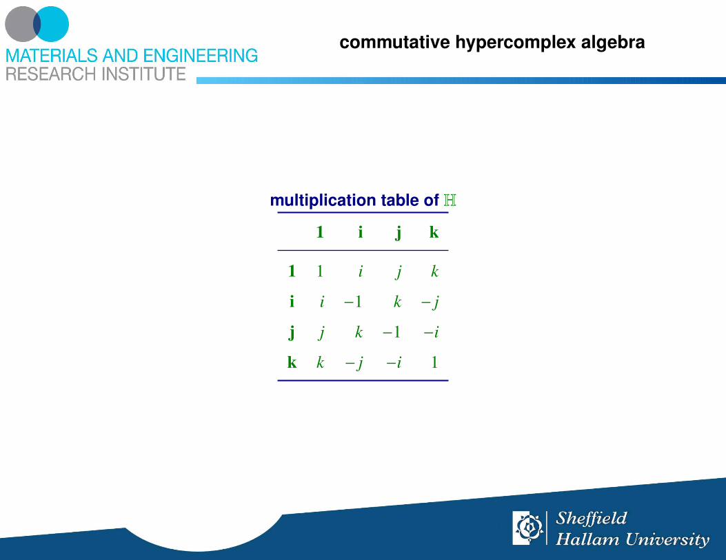
commutative hypercomplex algebra

multiplication table of H

1 i j k

1 1 i j k

i i −1 k − j

j j k −1 −i

k k − j −i 1

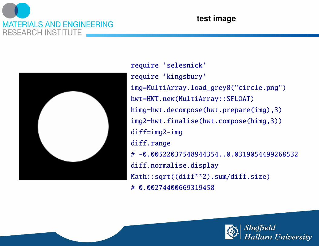
test image

require ’selesnick’

require ’kingsbury’

img=MultiArray.load_grey8("circle.png")

hwt=HWT.new(MultiArray::SFLOAT)

himg=hwt.decompose(hwt.prepare(img),3)

img2=hwt.finalise(hwt.compose(himg,3))

diff=img2-img

diff.range

# -0.00522037548944354..0.0319054499268532

diff.normalise.display

Math::sqrt((diff**2).sum/diff.size)

# 0.00274400669319458

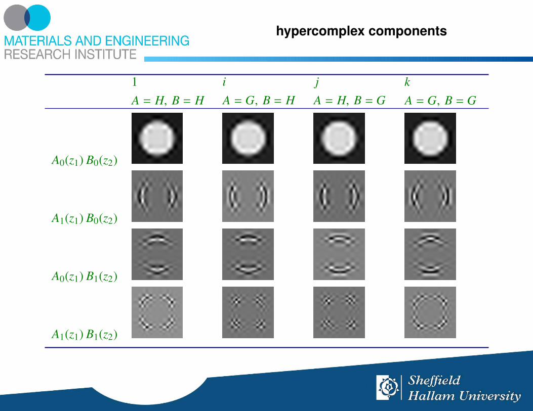
hypercomplex components

1A = H, B = H

iA = G, B = H

jA = H, B = G

kA = G, B = G

A0(z1) B0(z2)

A1(z1) B0(z2)

A0(z1) B1(z2)

A1(z1) B1(z2)

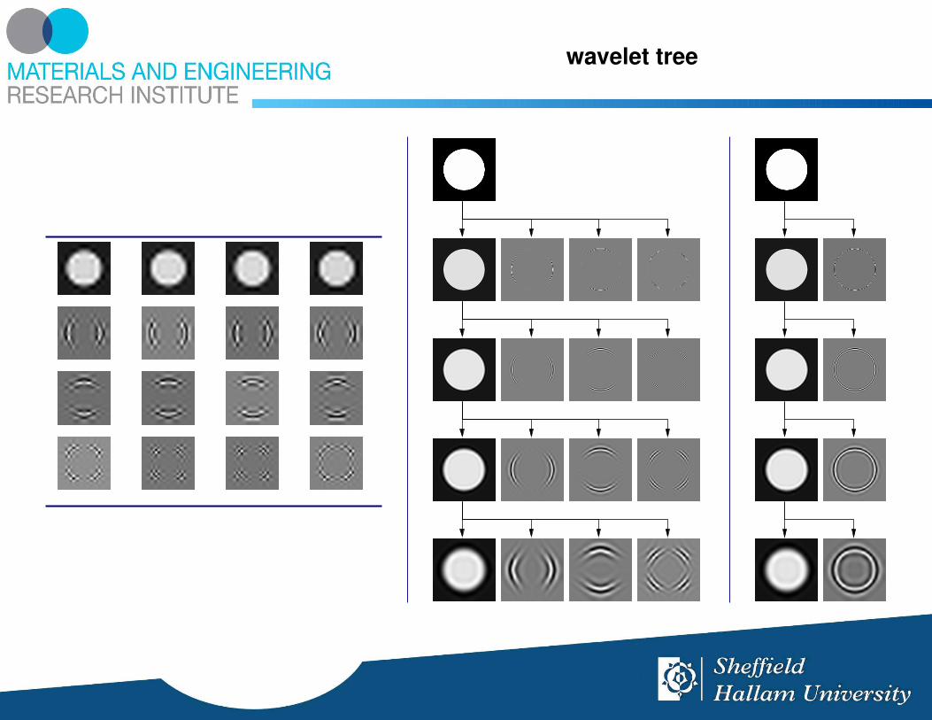
wavelet tree

linear combinations of 1-D basis wavelets

animating ∆x

10 i001

0i

V ′(z) =∑

a∈{0,1}

Ha(z)R(v′a)+

Ga(z)I(v′a)~v′ =

v′0v′1

= e

2 π∆x i/2 0

0 2 π∆x i

·

v0

v1

, ~v ∈ C2

animations require Javascript

2-D separable basis wavelets

1 0

0 0

i 0

0 0

j 0

0 0

k 0

0 0

0 1

0 0

0 i

0 0

0 j

0 0

0 k

0 0

0 0

1 0

0 0

i 0

0 0

j 0

0 0

k 0

0 0

0 1

0 0

0 i

0 0

0 j

0 0

0 k

linear combinations of 2-D basis wavelets

animation

V ′(z1, z2) =∑

a,b∈{0,1}

Ha(z1) Hb(z2)R(v′a,b)+

Ga(z1) Hb(z2)I(v′a,b)+

Ha(z1) Gb(z2)J(v′a,b)+

Ga(z1) Gb(z2)K(v′a,b)

V′ =e

2 π∆x2 j/2 0

0 2 π∆x2 j

· V·

e

2 π∆x1 i/2 0

0 2 π∆x1 i

, V ∈ C2×2

animations require Javascript

coping with rotations (Kingsbury) (Bharath,Ng)

Rotation-invariant local feature matchingwith complex wavelets

A steerable complex wavelet constructionand its application to image denoising

wavelet editor

blob-like pattern

(1 − k) cos(α)

1 0

0 0

+ (i − j) sin(α)

1 0

0 0

animations require Javascript

edge pattern

v1,0 v1,1

v0,1 ρ

(1 + k) cos(α + ρ)

0 1

0 0

+ (i + j) cos(α − ρ)

0 1

0 0

+(1 + k) sin(α + ρ)

0 0

1 0

+ (i + j) sin(α − ρ)

0 0

1 0

+12

(1 − i) sin(α)

0 0

0 1

+ 12

(1 − j) cos(α)

0 0

0 1

animations require Javascript

cross pattern

(1 + i + j + k) cos(α)

0 0

0 1

+(1 + i − j − k) sin(α)

0 0

1 0

+(−1 + i − j + k) sin(α)

0 1

0 0

cos(α)H1+sin(α)H2, where H1,H2 ∈ HCA2×2

animations require Javascript

conclusion

• improved understanding of high frequency pattern

• enable use of hypercomplex wavelets beyond edge detection

• several fully steerable patterns (translation, rotation)

• hypercomplex matrices for representing local structure

animations require Javascript

future work

• complete basis of steerable patterns? rotation around any point?

• understand interaction between neighbouring coefficients

• understand interaction of different layers of wavelet pyramid (Kingsbury)

• choose keypoints, descriptors

animations require Javascript

HornetseyeGPL (free and open source software)

http://rubyforge.org/projects/hornetseye/

http://sourceforge.net/projects/hornetseye/

http://vision.eng.shu.ac.uk/mediawiki/index.php/Hornetseye

http://raa.ruby-lang.org/project/hornetseye/

http://www.wedesoft.demon.co.uk/hornetseye-api/

filter design (Selesnick)

perfect reconstruction

recursionG0(z)

G1(z)

2 2G0(z)

G1(z) 2 2

recursion2 2H0(z)

H1(z) 2 2

H0(z)

H1(z)

Thiran filter (τ = 0.5)d(n) =

(L−1

n

)(−1)n∏n−1

k=0τ−L+1+kτ+1+k

vanishing moments

K = 1 1 − 1

K = 2 1 − 2 1

K = 3 1 − 3 3 − 1

K = 4 1 − 4 6 − 4 1

. . . . . .

12(H0(z)X(z) + H0(−z)X(−z)

)H0(z)+

12(H1(z)X(z) + H1(−z)X(−z)

)H1(z) =(∗) X(z)

⇔

H0(z) H0(−z) + H1(z) H1(−z) = 0 (1)

H0(z) H0(z) + H1(z) H1(z) = 2 (2)

⇐

H1(z) = H0(−z)

H1(z) = −H0(−z)(1)X

H0(z) = Q(z) (1 + z−1)K D(z)

H0(z) = Q(z) (1 + z−1)K D(z−1) z1−L(2)· · ·

(∗) [↑ 2]([↓ 2](x(n))) c ........... s 1

2(X(z) + X(−z)

)

filter design (Selesnick)

perfect reconstruction

recursionG0(z)

G1(z)

2 2G0(z)

G1(z) 2 2

recursion2 2H0(z)

H1(z) 2 2

H0(z)

H1(z)

Thiran filter (τ = 0.5)d(n) =

(L−1

n

)(−1)n∏n−1

k=0τ−L+1+kτ+1+k

vanishing moments

K = 1 1 − 1

K = 2 1 − 2 1

K = 3 1 − 3 3 − 1

K = 4 1 − 4 6 − 4 1

. . . . . .

12(G0(z)X(z) + G0(−z)X(−z)

)G0(z)+

12(G1(z)X(z) + G1(−z)X(−z)

)G1(z) =(∗) X(z)

⇔

G0(z) G0(−z) + G1(z) G1(−z) = 0 (3)

G0(z) G0(z) + G1(z) G1(z) = 2 (4)

⇐

G1(z) = G0(−z)

G1(z) = −G0(−z)(3)X

G0(z) = Q(z) (1 + z−1)K D(z−1) z1−L

G0(z) = Q(z) (1 + z−1)K D(z)(4)· · ·

(∗) [↑ 2]([↓ 2](x(n))) c ........... s 1

2(X(z) + X(−z)

)

filter design (Selesnick)

(2)· · ·

H0(z) H0(z) + H1(z) H1(z) = 2

H1(z) = H0(−z)

H1(z) = −H0(−z)

H0(z) = Q(z) (1 + z−1)K D(z)

H0(z) = Q(z) (1 + z−1)K D(z−1) z1−L

1 = H0(z) H0(z) = (1 + z−1)K+K D(z) D(z−1) z1−L︸ ︷︷ ︸

CS (z)

Q(z) Q(z)︸ ︷︷ ︸CR(z)

filter design (Selesnick)

(4)· · ·

G0(z) G0(z) + G1(z) G1(z) = 2

G1(z) = G0(−z)

G1(z) = −G0(−z)

G0(z) = Q(z) (1 + z−1)K D(z−1) z1−L

G0(z) = Q(z) (1 + z−1)K D(z)

1 = G0(z) G0(z) = (1 + z−1)K+K D(z) D(z−1) z1−L︸ ︷︷ ︸

CS (z)

Q(z) Q(z)︸ ︷︷ ︸CR(z)

filter design (Selesnick)

(2,4)· · ·

S (z) Q(z) Q(z)︸ ︷︷ ︸R(z)

= 1⇔

sN 0 · · ·

sN−2 sN−1 sN 0 · · ·

......

.........

· · · 0 s1 s2 s3

· · · 0 s1

r1

r2...

rN−1

rN

=

...

0

1

0...

{ R(z)

spectral factorisation (Laguerre)

Laguerre

Input: Polynomial p(x)Output: zero crossing o ∈ C of px 7→ 0.0 + 0.0 i; c 7→ 100;while c ≥ 0 do

if |p(x)| sufficiently small thenreturn o = x;

endg = p′(x)/p(x);h = g2 − p′′(x)/p(x);if |g + d| > |g − d| then

a = n/(g + d);else

a = n/(g − d);endx 7→ x − a; c 7→ c − 1;

end

spectral factorisationR(z) symmetric, real-valued

Re

Im

tuples

Re

quadruples

Im

Re

Im

tuples

Re

quadruples

Im

Re

Im

tuples

Re

quadruples

Im

Q(z) Q(z)H0(z) = Q(z) (1 + z−1)K D(z)H0(z) = Q(z) (1 + z−1)K D(z−1) z1−L

H1(z) = H0(−z), H1(z) = −H0(−z)(2,4)X