Open University Malaysia

Faculty Science and Technology

Diploma in Mechanical Engineering

Subject Advance Fluid Mechanics For Mechanical Engineering

Code EDMFS3103

Semester September Date: 19/10/08

A. Information on Students

EXPERIMENT 1: PERFORMANCE OF A STEAM POWER PLANT OBJECTIVE OF EXPERIMENT: This experiment is to acquire experience on the operation of a functional steam turbine

power plant and understanding of simple Rankine cycle. A comparison of a real world

operating characteristics to that of the ideal Rankine power cycle will be made and

identification factors and parameters affecting the cycle efficiency. In this experiment, we

will determine:

aa)) Thermodynamics properties (entropies, enthalpies, quality, etc). Draw a

schematic of the cycle in a T-S diagram.

bb)) Thermal efficiency of the cycle.

cc)) Mass flow rate steam in the turbine.

Theory

The Rankine cycle is the most common of all power generation cycles as shown in

Figures 1 and 2. The Rankine cycle was devised to make use of the characteristics of

water as the working fluid. The cycle begins in a boiler (State 3 in figure 1), where the

water is heated until it reaches saturation- in a constant-pressure process. Once

saturation is reached, further heat transfer takes place at a constant temperature, until

the working fluid reaches a quality of 100% (State 4). At this point, the high-quality

vapor is expanded isoentropically through an axially bladed turbine stage to produce

shaft work. The steam then exits the turbine at State 5.

The working fluid, at State 5, is at a low-pressure, but has a fairly high quality, so it is

routed through a condenser, where the steam is condensed into liquid (State 1). Finally,

the cycle is completed via the return of the liquid to the boiler, which is normally

accomplished by a mechanical pump. Figure 2 shows a schematic of a power plant

under a Rankine cycle.

Figure 1: Diagrams for a simple ideal Rankine cycle:

a) P-V diagram, b) T-S diagram

1

2

3 4

5 1

2 3

4

5

The area under the process curve in the T – s diagram represents the heat

transfer for an internally reversible process. The area under the process curve from

state 2 to state 4 is the heat transferred to the water in the boiler. The area under the

process curve from state 5 to state 1 is the heat rejected in the condenser. The

difference between the two (the area within the process cycle) represents the net work

produced by the cycle.

To perform the thermodynamic analysis on the ideal cycle each component is

modeled as a control volume. All processes are executed in steady-flow sections and

can be analyzed as a steady-flow process, expressed on a basis of unit mass as q – w =

hexit – hinlet. The boiler and condenser do not involve work and the turbine is considered

to be isentropic. Additionally, there is one flow in to each device and one flow out of

each device. Under consideration of all of these conditions the specific first law analysis

for each device is:

Pump (q = 0): win,PUMP = h2 – h1

Boiler (w = 0): qin = h4 – h3

Turbine (q = 0): wout,TURB = h4 – h5

Condenser (w = 0): qout = h4 – h1

The thermal efficiency of the Rankine cycle is determined from: in

out

in

netth

q

q

q

w 1

Where wnet = qin – qout = wout,TURB – win,PUMP

Figure 2: Diagrams for a Typical Steam Plant cycle

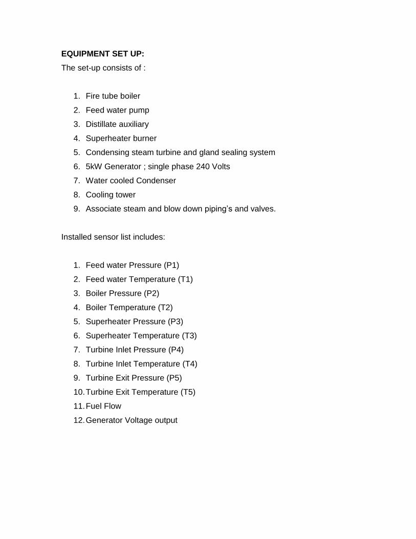
EQUIPMENT SET UP:

The set-up consists of :

1. Fire tube boiler

2. Feed water pump

3. Distillate auxiliary

4. Superheater burner

5. Condensing steam turbine and gland sealing system

6. 5kW Generator ; single phase 240 Volts

7. Water cooled Condenser

8. Cooling tower

9. Associate steam and blow down piping’s and valves.

Installed sensor list includes:

1. Feed water Pressure (P1)

2. Feed water Temperature (T1)

3. Boiler Pressure (P2)

4. Boiler Temperature (T2)

5. Superheater Pressure (P3)

6. Superheater Temperature (T3)

7. Turbine Inlet Pressure (P4)

8. Turbine Inlet Temperature (T4)

9. Turbine Exit Pressure (P5)

10. Turbine Exit Temperature (T5)

11. Fuel Flow

12. Generator Voltage output

Figure 3: Schematic of Rankine cycle steam turbine apparatus

Turbine Exit

pressure &Temp (P5

& T5)

Turbine Inlet

pressure &Temp (P4

& T4)

Feed water pressure

/Temp (P2 & T2)

Superheater

Fuel oil /

Diesel

Water tank

Feed water pressure

/Temp (P1 & T1)

Boiler pressure &Temp

(P3 & T3)

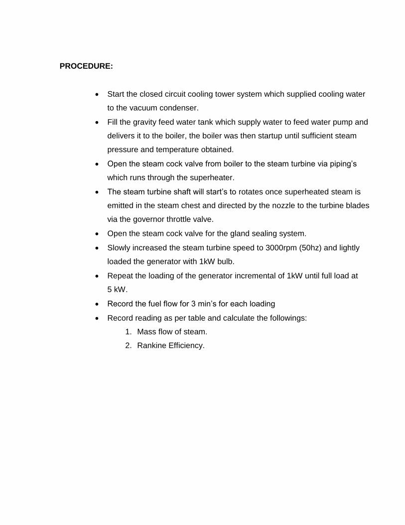
PROCEDURE:

Start the closed circuit cooling tower system which supplied cooling water

to the vacuum condenser.

Fill the gravity feed water tank which supply water to feed water pump and

delivers it to the boiler, the boiler was then startup until sufficient steam

pressure and temperature obtained.

Open the steam cock valve from boiler to the steam turbine via piping’s

which runs through the superheater.

The steam turbine shaft will start’s to rotates once superheated steam is

emitted in the steam chest and directed by the nozzle to the turbine blades

via the governor throttle valve.

Open the steam cock valve for the gland sealing system.

Slowly increased the steam turbine speed to 3000rpm (50hz) and lightly

loaded the generator with 1kW bulb.

Repeat the loading of the generator incremental of 1kW until full load at

5 kW.

Record the fuel flow for 3 min’s for each loading

Record reading as per table and calculate the followings:

1. Mass flow of steam.

2. Rankine Efficiency.

Result:

Electrical power demand (kW) 1 2 3 4 5

Voltage(V) 225 210 215 210 170

Current(I) 5.1 10.1 15 17.6 18.5

Power output(P=V x I) Watt 1147.5 2121 3225 3696 3145

Fuel Consumption in boiler (kg) / 10 mins 1.7 2.1 2.3 2.4 2.8

P1 (bar) 1 1 1 1 1

P2(bar) 10.3 10.3 8 8 8

P3(bar) 8 7.5 7 7 6.5

P4(bar) 2.55 3 4.7 6 5.5

P5(bar) -0.25 -0.15 0 0.25 0.15

T1(°c) 29 29 29 29 29

T2(°c) 170 174 171 170 170

T3(°c) 170 174 171 170 170

T4(°c) 300 302 280 259 264

T5(°c) 58 64 74 82 80

h1(kJ/kg) 417.4365 417.4365 417.4365 417.4365 417.4365

h2(kJ/kg) 417.4365 417.4365 417.4365 417.4365 417.4365

h3(kJ/kg) 2768.302 2765.641 2762.749 2762.749 2759.595

h4(kJ/kg) 3070.7249 3073.6852 3024.1257 2976.5448 2988.5986

h5(kJ/kg) 2605.359 2615.784 2632.909 2646.351 2643.014

h2 - h1 (kJ/kg) Work done by pump is neglected

h4 - h5 (kJ/kg) 465.3656 457.9017 391.2167 330.1933 345.5843

h4 - h2 (kJ/kg) 2605.3592 2656.2487 2606.6892 2559.1083 2571.1622

Mass flow rate of steam, ms (x 10-3

kg/s) 2.465803 4.631999 8.243512 11.19344 9.100529

Mass flow rate of diesel, mf (x 10-3

kg/s) 2.833333 3.500000 3.833333 4.000000 4.666667

Rankine efficiency (%) 17.86186 17.23866 15.00819 12.90267 13.44078

Figure 4: T-S diagram

Diagrams for a experiment Rankine cycle:

Rankine cycle analysis

This experiment has an important difference with the cycle shown in Figure 2. The

difference is that there is no pump to complete the cycle. This is not exactly a cycle.

Instead, it is an open system. The steam crossing the condenser i.e condensate is

stored in a tank as show in Figure 3, but the principle of Rankine cycle studied in

Thermodynamic is still valid.

The boiler will be filled with water before the experiment and the experiment will be

ended when the water is reaches the minimum level of correct operation, given by the

demonstrator.

Another important difference is that between the boiler and turbine there is a valve that

generates a throttling effect. The throttling process is analyzed as an isenthalpic

process. Also, the boiler generates a superheated vapor.

S

1

2 3

4

5

T

II.. Mass flow rate in the turbine

From the generated amperage and voltage:

VIWt

so, the mass flow rate in the turbine is:

54 hh

VIm

t

Where t is the efficiency of the turbine. Here, we will assume this efficiency equal to

one.

IIII.. Rankine Efficiency of Cycle

The net work of the cycle is defined by the difference between the turbine work and the

pump work:

1254 hhmhhmWWW waterwaterptcycle

If the pump work is neglected, the net work of the cycle reduces to:

54 hhmW watercycle

Then the thermal efficiency of this system is defined by the rate between the net work

and heat transfer from the boiler:

24

54

hh

hh

Q

W

in

t

Assumption:

1. Each component of the cycle is analyzed at steady state.

2. Constant pressure heat rejection.

3. The turbine and pump operate adiabatically (Constant pressure heat addition).

4. Kinetic and potential energy effects are negligible.

5. Superheated vapor enters the turbine.

6. Condensate exits the condenser as saturated liquid.

7. x =1

Analysis:

State 1, condenser outlet - pump inlet:

kg

mvv

kg

kJhhabsbarpsigp ff

3

111 001049.0,3.448_291.1042.4

State 3, boiler outlet - turbine inlet:

Kkg

kJs

kg

kJhCTabsbarpsigp

202.7,1.27275.129,_903.1924.12 3333

State 4, turbine outlet – condenser inlet:

kg

kJhCTabsbarpp 4.27223.124,_291.1 4414

Process 1-2, pump:

absbarpp _903.132

Because the pump is assumed isentropic

kWkPakPakg

m

s

kgppvmW PUMPinnet 06420.01.1293.190001049.000.1

3

121,,

kg

kJ

s

kg

kWkg

kJ

s

kg

m

Whmh innet 4.448

00.1

06420.03.44800.1,1

2

Process 2-3, boiler:

kWkg

kJ

kg

kJ

s

kghhmQ BOILERinnet 7.22784.4481.272700.123,,

Process 3-4, turbine:

kWkg

kJ

kg

kJ

s

kghhmW TURBoutnet 6181.44.27221.272700.143,,

Process 4-1, condenser:

kWkg

kJ

kg

kJ

s

kghhmQ CONDinnet 1.22744.27223.44800.141,,

Generator power

WVAmpIVPgen 756.0032.2372.0

Net work

kWkWkWWWW PUMPinnetTURBoutnetoutnet 5539.406420.06181.4,,,,,

Overall thermal efficiency

%200.01007.2278

5539.4100

,,

,

kW

kW

Q

W

BOILERinnet

outnet

Observation: The thermal efficiency of this Rankine cycle is very small compared to the

efficiencies obtained in power plants that use the Rankine cycle. The thermal

efficiencies for the cycle ranged from 0.123% to 0.200%, whereas a power plant might

have efficiencies of around 25-30%. The generator efficiency was even smaller than the

thermal efficiency, suggesting that the generator is not producing much power from the

shaft rotation. The turbine isentropic efficiencies were around 5-7%, suggesting that

there is much heat loss and friction in the turbine, resulting in much irreversibility. There

are many other possible explanations for the small efficiencies obtained. It may not be

accurate to compare a Rankine cycle of this size to a power plant cycle. The small size

of the Rankine cycle test device is probably not the proper or ideal size for a practical

Rankine cycle plant. It is possible that much of the heat of the propane combustion is

wasted since the boiler may not be large enough to facilitate the efficient transfer of heat

from the combustion to the water and steam. Heat and pressure losses from the boiler

are probably significant, although there was no apparent way to measure these losses,

so the analysis assumes that they do not occur. It is also likely that the fuel may not

entirely combust, or the density and heating value of the propane used in the experiment

may be different from the values used in the analysis. Significant pressure losses

probably also occur in the cooling tower, although constant pressure heat rejection is

assumed in the analysis. The assumption that the water leaves the condenser as a

saturated liquid may not be valid if the cooling tower does not efficiently reject the heat.

The large steam loss from the cooling tower and other components decreases the mass

flow rate, which decreases the work produced by the turbine and reduces the thermal

efficiency of the cycle. The lower mass flow rate is probably not the optimum flow for

the boiler or turbine, resulting in irreversibilities and less efficiency for the components.

The steam loss made it difficult to achieve the desired generator power output since the

turbine was producing less shaft work. Heat and pressure losses also likely occur in the

pipes and valves connecting the prime movers. The significant drop in temperature from

the boiler outlet to the turbine inlet exemplifies these losses, which result in lost work

potential and lower efficiency. The steam loss rate is probably smaller than the

calculated value since the cycle was losing steam before data collecting began. The

cycle had to achieve a relatively steady state before the data collecting could begin.

Contaminants in the water, such as oil, may have altered the properties of the water,

affecting the work output and efficiencies.

Other possible sources of error may relate to the calculation or measuring

instruments. Precision limitations of the thermocouples, fuel flow sensor, or graduated

cylinders limited the accuracy of the first-law calculations and the steam loss rate.

Interpolations and rounding of values using property tables also contribute to precision

errors.

1. The experiment conducted was not so accurate due to leakage during

collection of water in the metering hydraulic bench. As a result collection time

was extended and this cause uncertainty in Re due to the uncertainty in both

volume and time measurements to calculate the average flow velocity which

was use for Re numbers calculation.

2. The uncertainty in the friction factor is similarly related to measurement of

volume and time because velocity is used in its calculation, and also affected

by the measured pressure difference.

3. There was error in the collection of pressure measurements, as the level in the

manometer not stabilized and the instantaneous reading made inaccurate and

also made the simultaneous reading of both pressure impossible.

Conclusion

Graph log LH versus log Q

From graph log LH versus log Q we can know the minor loss in the pipe system

due to sudden change in flow direction as in the entrance flow. The friction loss is

proportional to the pipe length, while minor losses can be emulated by sudden

pressure drop. In this case, we can summarize that minor losses represent

pressure losses in developing flow which is experiencing disturbances and

changes in internal pipe geometry.

Comparison of the graph.

From the graph we understand that the high flow and slow flow along a pipe. The

case that can cause minor loss is valve. The valve may only have two positions,

either open or close, or may be able to vary the flow rate. In valve, minor loss is

only generated when it is at lease partially open. It reduces the flow rate of a fluid

by reducing the opening. With combination of it internal geometry as radius, the

reduction of the opening generates a high pressure loss and thus reducing the

flow velocity.