statistics for managers using microsoft excel/spss · 10/02/2016 · anova and other c-sample tests...
TRANSCRIPT

© 1999 Prentice-Hall, Inc. Chap. 10 - 1
Statistics for Managers
Using Microsoft Excel/SPSS
Chapter 10
ANOVA and Other C-Sample
Tests With Numerical Data

© 1999 Prentice-Hall, Inc. Chap. 10 - 2
• The Completely Randomized Model: One-Factor Analysis of Variance
F-Test for Difference in c Means
The Tukey-Kramer Procedure
ANOVA Assumptions
• The Factorial Design Model: Two-Way Analysis of Variance
Examine Effect of Factors and Interaction
• Kruksal-Wallis Rank Test for Differences in c
Medians
Chapter Topics

© 1999 Prentice-Hall, Inc. Chap. 10 - 3
One-Factor
Analysis of Variance
• Evaluate the Difference Among the
Means of 2 or More (c) Populations
e.g., Several Types of Tires, Oven Temperature Settings
• Assumptions:
Samples are Randomly and Independently Drawn
(This condition must be met.)
Populations are Normally Distributed
(F test is Robust to moderate departures from
normality.)
Populations have Equal Variances

© 1999 Prentice-Hall, Inc. Chap. 10 - 4
One-Factor ANOVA Test Hypothesis
H0: m1 = m2 = m3 = ... = mc
•All population means are equal
•No treatment effect (NO variation in means
among groups)
H1: not all the mk are equal
•At least ONE population mean is different
(Others may be the same!)
•There is treatment effect
Does NOT mean that all the means are different:
m1 m2 ... mc

© 1999 Prentice-Hall, Inc. Chap. 10 - 5
One-Factor ANOVA: No Treatment Effect
m1 = m2 = m3
H0: m1 = m2 = m3 = ... = mc
H1: not all the mk are equal
The Null
Hypothesis is
True

© 1999 Prentice-Hall, Inc. Chap. 10 - 6
One Factor ANOVA: Treatment Effect Present
m1 = m2 m3
H0: m1 = m2 = m3 = ... = mc
H1: not all the mk are equal The Null
Hypothesis is
NOT True

© 1999 Prentice-Hall, Inc. Chap. 10 - 7
One-Factor ANOVA
Partitions of Total Variation
Variation Due to
Treatment SSA
Variation Due to Random
Sampling SSW
Total Variation SST
Commonly referred to as:
Sum of Squares Within, or
Sum of Squares Error, or
Within Groups Variation
Commonly referred to as:
Sum of Squares Among, or
Sum of Squares Between, or
Sum of Squares Model, or
Among Groups Variation
= +
© 1999 Prentice-Hall, Inc. Chap. 10 - 8
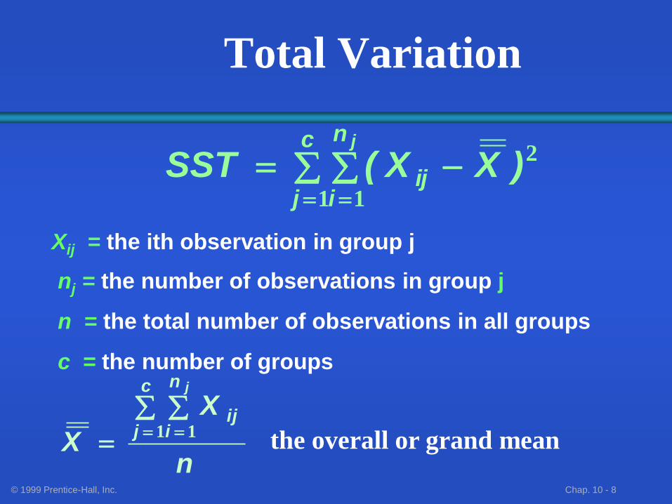
Total Variation
2
1 1
)XX(SSTc
j
n
iij
j
== =
n
X
X
c
j
n
iij
j
== =1 1 the overall or grand mean
Xij = the ith observation in group j
nj = the number of observations in group j
n = the total number of observations in all groups
c = the number of groups

© 1999 Prentice-Hall, Inc. Chap. 10 - 9
Among-Group Variation
2
1
)XX(nSSA j
c
jj =
=
nj = the number of observations in group j
c = the number of groups
the sample mean of group j
the overall or grand mean
mi mj
Variation Due to Differences Among Groups.
1=
c
SSAMSA
Xj
X
_
_ _

© 1999 Prentice-Hall, Inc. Chap. 10 - 10
Within-Group Variation
2
1 1
)XX(SSW j
c
j
n
iij
j
== =
=ijX the ith observation in group j
=jX the sample mean of group j
m j
Summing the variation within
each group and then adding
over all groups.
cn
SSWMSW
=

© 1999 Prentice-Hall, Inc. Chap. 10 - 11
Within-Group Variation
m j
)n()n()n(
S)n(S)n(S)n(
cn
SSWMSW
c
cc
111
111
21
2222
211
=
=
For c = 2, this is the
pooled-variance in the
t-Test.
•If more than 2 groups,
use F Test.
•For 2 groups, use t-Test.
F Test more limited.

© 1999 Prentice-Hall, Inc. Chap. 10 - 12
One-Way ANOVA
Summary Table
Source of Variation
Degrees of
Freedom
Sum of Squares
Mean Square
(Variance)
Among (Factor)
c - 1 SSA MSA = SSA/(c - 1)
MSA
MSW
Within (Error)
n - c SSW MSW = SSW/(n - c)
Total n - 1 SST = SSA+SSW
F Test
Statistic
=

© 1999 Prentice-Hall, Inc. Chap. 10 - 13
One-Factor ANOVA
F Test Example
As production manager, you
want to see if 3 filling
machines have different mean
filling times. You assign 15
similarly trained &
experienced workers, 5 per
machine, to the machines. At
the .05 level, is there a
difference in mean filling
times?
Machine1 Machine2
Machine3
25.40 23.40 20.00
26.31 21.80 22.20
24.10 23.50 19.75
23.74 22.75 20.60
25.10 21.60 20.40

© 1999 Prentice-Hall, Inc. Chap. 10 - 14
One-Factor ANOVA
Example: Scatter Diagram
27
26
25
24
23
22
21
20
19
• •
• •
•
• •
•
• •
• • • •
•
X
X
x
x
X = 24.93 X = 22.61 X = 20.59
X = 22.71
Machine1 Machine2
Machine3
25.40 23.40 20.00
26.31 21.80 22.20
24.10 23.50 19.75
23.74 22.75 20.60
25.10 21.60 20.40
_ _
_ _
_ _ _
_
_
_

© 1999 Prentice-Hall, Inc. Chap. 10 - 15
One-Factor ANOVA
Example Computations
X1 = 24.93
X2 = 22.61
X3 = 20.59
X = 22.71
SSA = 5 [(24.93 - 22.71) 2+ (22.61 - 22.71)2 + (20.59 - 22.71) 2]
= 47.164
SSW = 4.2592+3.112 +3.682 = 11.0532
MSA = SSA/(c-1) = 47.16/2 = 23.5820
MSW = SSW/(n-c) = 11.0532/12 = .9211
nj =5
c = 3
n = 15
Machine1 Machine2
Machine3
25.40 23.40 20.00
26.31 21.80 22.20
24.10 23.50 19.75
23.74 22.75 20.60
25.10 21.60 20.40
_
_
_
_
_

© 1999 Prentice-Hall, Inc. Chap. 10 - 16
Summary Table
Source of Variation
Degrees of Freedom
Sum of Squares
Mean Square
(Variance)
F =
= 25.60
Among (Machines)
3 - 1 = 2 47.1640 23.5820
Within (Error)
15 - 3 = 12 11.0532 .9211
Total 15 - 1 = 14 58.2172
MSA
MSW

© 1999 Prentice-Hall, Inc. Chap. 10 - 17
F 0 3.89
One-Factor ANOVA
Example Solution H0: m1 = m2 = m3
H1: Not All Equal
a = .05
df1= 2 df2 = 12
Critical Value(s):
Test Statistic:
Decision:
Conclusion:
Reject at a = 0.05
There is evidence that at least
one m i differs from the rest.
a = 0.05
F MSA
MSW = = =
23 5820
9211 25 6
.
. .
© 1999 Prentice-Hall, Inc. Chap. 10 - 18
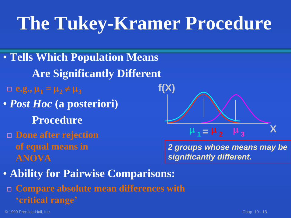
The Tukey-Kramer Procedure
• Tells Which Population Means
Are Significantly Different
e.g., m1 = m2 m3
• Post Hoc (a posteriori)
Procedure
Done after rejection
of equal means in
ANOVA
• Ability for Pairwise Comparisons:
Compare absolute mean differences with
‘critical range’
X
f(X)
m 1 = m
2 m
3
2 groups whose means may be
significantly different.

© 1999 Prentice-Hall, Inc. Chap. 10 - 19
The Tukey-Kramer Procedure:
Example 1. Compute absolute mean
differences:
Machine1 Machine2 Machine3
25.40 23.40 20.00
26.31 21.80 22.20
24.10 23.50 19.75
23.74 22.75 20.60
25.10 21.60 20.40 02259206122
34459209324
32261229324
32
31
21
...XX
...XX
...XX
==
==
==
2. Compute Critical Range:
3. Each of the absolute mean difference is greater. There is a
significance difference between each pair of means.
=
'jj
)cn,c(Unn
MSWQRangeCritical
11
2= 1.618

© 1999 Prentice-Hall, Inc. Chap. 10 - 20
Two-Way ANOVA
• Examines the Effect of:
Two Factors on the Dependent Variable
e.g., Percent Carbonation and Line Speed on
Soft Drink Bottling Process
Interaction Between the Different Levels of
these Two Factors
e.g., Does the effect of one particular
percentage of Carbonation depend on
which level the line speed is set?

© 1999 Prentice-Hall, Inc. Chap. 10 - 21
Two-Way ANOVA
Assumptions
• Normality
Populations are normally distributed
• Homogeneity of Variance
Populations have equal variances
• Independence of Errors
Independent random samples are drawn

© 1999 Prentice-Hall, Inc. Chap. 10 - 22
Two-Way ANOVA
Total Variation Partitioning
Variation Due to
Treatment A
Variation Due to
Random Sampling
Variation Due to
Interaction
SSE
SSFA +
SSAB + SST =
Variation Due to
Treatment B SSFB +
Total Variation
© 1999 Prentice-Hall, Inc. Chap. 10 - 23
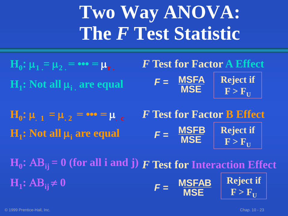
Two Way ANOVA: The F Test Statistic
F Test for Factor A Effect
MSFA MSE
F =
F Test for Factor B Effect
F = MSFB MSE
F Test for Interaction Effect
F = MSFAB MSE
H0: m1 .= m2 . = ••• = mr .
H1: Not all mi . are equal
H0: ABij = 0 (for all i and j)
H1: ABij 0
H0: m. 1 = m. 2 = ••• = m. c
H1: Not all mi are equal
Reject if
F > FU
Reject if
F > FU
Reject if
F > FU

© 1999 Prentice-Hall, Inc. Chap. 10 - 24
Source of Variation
Degrees of Freedom
Sum of Squares
Mean Square F Statistic:
A (Row)
r - 1 SSFA MSFA MSFA
MSE
B (Column)
c - 1 SSFB MSFB MSFB
MSE
AB (Interaction)
(r-1)(c-1) SSAB MSAB MSAB
MSE
Error r·c·(n’-1) SSE MSE
Total r·c·n’ - 1 SST
Two-Way ANOVA
Summary Table
=
=
=

© 1999 Prentice-Hall, Inc. Chap. 10 - 25
Kruskal-Wallis Rank
Test for c Medians
• Extension of Wilcoxon Rank Sum Test
Tests the equality of more than 2 (c)
population medians
• Distribution-free test procedure
• Used to analyze completely randomized
experimental designs
• Use c2 distribution to approximate if each
sample group size nj > 5, df = c - 1

© 1999 Prentice-Hall, Inc. Chap. 10 - 26
Kruskal-Wallis Rank
Test • Assumptions:
Independent random samples are drawn
Continuous dependent variable
Data may be ranked both within and among samples
Populations have same variability
Populations have same shape
• Robust with regard to last 2 conditions
Use F Test in completely randomized designs and when the more stringent assumptions hold.
© 1999 Prentice-Hall, Inc. Chap. 10 - 27
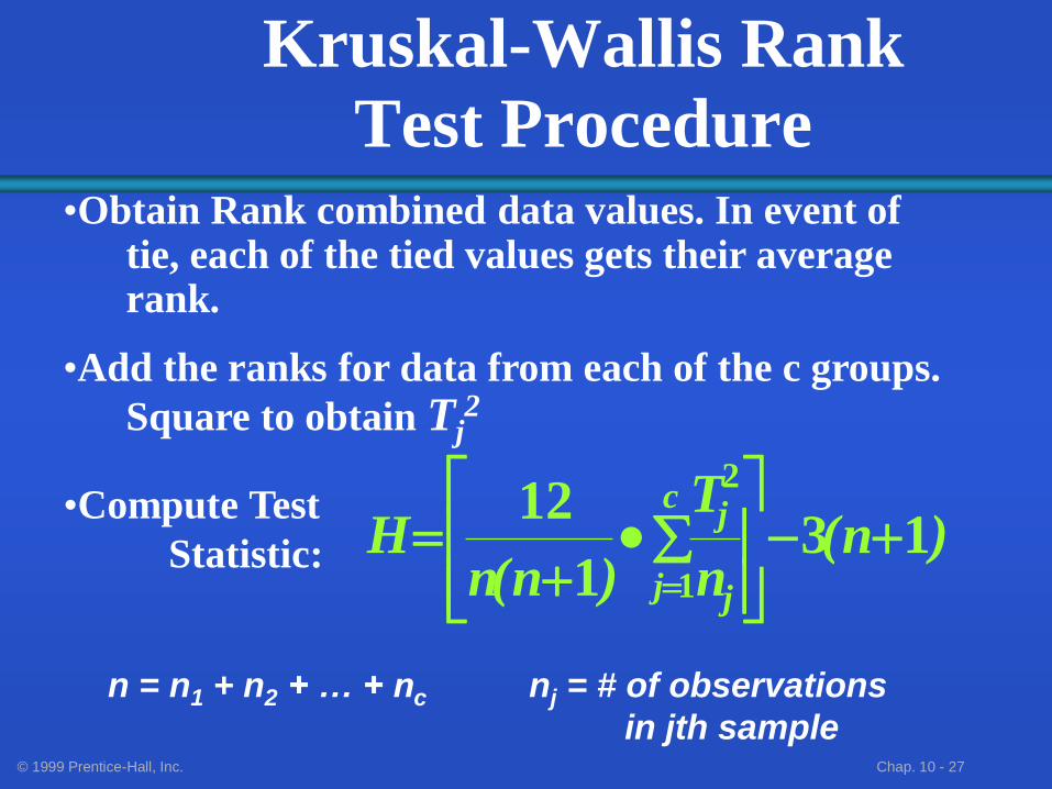
Kruskal-Wallis Rank
Test Procedure •Obtain Rank combined data values. In event of tie, each of the tied values gets their average rank.
•Add the ranks for data from each of the c groups.
Square to obtain Tj2
n = n1 + n2 + … + nc nj = # of observations
in jth sample
•Compute Test
Statistic: )n(n
T
)n(nH
c
j j
j13
1
12
1
2
=
=

© 1999 Prentice-Hall, Inc. Chap. 10 - 28
Kruskal-Wallis Rank
Test Procedure
•Test Statistic, H may be approximated by Chi-
square distribution (df = c -1)
•Critical Value for a given a: Upper tail
•Decision Rule: Reject H0: M1 = M2 = ••• = Mc
if Test Statistic H >
otherwise do not reject H0
2cU
2cU

© 1999 Prentice-Hall, Inc. Chap. 10 - 29
As production manager, you
want to see if 3 filling
machines have different
median filling times. You
assign 15 similarly trained &
experienced workers,
5 per machine, to the machines.
At the .05 level, is there a
difference in median filling
times?
Kruksal-Wallis Rank Test:
Example
Machine1 Machine2
Machine3
25.40 23.40 20.00
26.31 21.80 22.20
24.10 23.50 19.75
23.74 22.75 20.60
25.10 21.60 20.40

© 1999 Prentice-Hall, Inc. Chap. 10 - 30
Example Solution: Step 1
Obtaining a Ranking
Raw Data Ranks
65 38 17
Machine1 Machine2
Machine3
25.40 23.40 20.00
26.31 21.80 22.20
24.10 23.50 19.75
23.74 22.75 20.60
25.10 21.60 20.40
Machine1 Machine2
Machine3
14 9
2 15 6
7
12 10 1
11 8 4
13 5 3

© 1999 Prentice-Hall, Inc. Chap. 10 - 31
Example Solution: Step 2
Test Statistic Computation
)n(c
j jn
jT
)n(nH 13
1
2
112
=
=
)()(
11535
17
5
38
5
65
11515
12222
=
= 11.58

© 1999 Prentice-Hall, Inc. Chap. 10 - 32
H0: M1 = M2 = M3
H1: Not all equal
a = .05
df = c - 1 = 3 - 1 = 2
Critical Value(s):
Reject at
c 20 5.991 c 20 5.991
H = 1158.H = 1158.
Kruskal-Wallis Test
Example Solution
Test Statistic:
Decision:
Conclusion:
There is evidence that
population medians are
not all equal.
a = .05
a = .05
© 1999 Prentice-Hall, Inc. Chap. 10 - 33
• Described The Completely Randomized Model: One-Factor Analysis of Variance
F-Test for Difference in c Means
The Tukey-Kramer Procedure
ANOVA Assumptions
• Discussed The Factorial Design Model: Two-Way Analysis of Variance
Examined effect of Factors and Interaction
• Addressed the Kruskal-Wallis Rank Test for Differences in c Medians
Chapter Summary