statistics for managers using microsoft® excel 5th … series...moving averages used for smoothing...

1

Statistics for Managers Using Microsoft Excel, 5e © 2008 Prentice-Hall, Inc. Chap 16-1

Statistics for ManagersUsing Microsoft® Excel

5th Edition

Chapter 16

Time-Series Forecasting and IndexNumbers


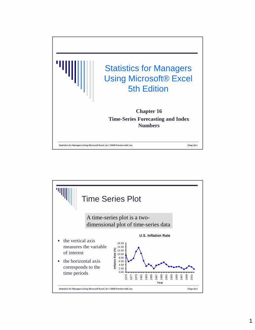
Time Series Plot

the vertical axismeasures the variableof interest

the horizontal axiscorresponds to thetime periods

U.S. Inflation Rate

0.002.004.006.008.00

10.0012.0014.0016.00

1975

1977

1979

1981

1983

1985

1987

1989

1991

1993

1995

1997

1999

2001

Year

Infla

tion

Rat

e (%

)

A time-series plot is a two-dimensional plot of time-series data

2

Class Exercise



Time-Series Components

Time Series

CyclicalComponent

IrregularComponent

TrendComponent

SeasonalComponent

3


Trend Component

Long-run increase or decrease over time (overallupward or downward movement)

Data taken over a long period of time

Sales

Time


Trend Component

Trend can be upward or downward

Trend can be linear or non-linear

Downward linear trend

Sales

TimeUpward nonlinear trend

Sales

Time

4


Seasonal Component Short-term regular wave-like patterns

Observed within 1 year

Often monthly or quarterly

Sales

Time (Quarterly)

Winter

Spring

Summer

Fall

Winter

Spring

Summer

Fall


Cyclical Component Long-term wave-like patterns

Regularly occur but may vary in length

Often measured peak to peak or trough to trough

Sales1 Cycle

Year

5


Irregular Component

Unpredictable, random, “residual”fluctuations

Due to random variations of Nature

Accidents or unusual events

“Noise” in the time series


Multiplicative Time-SeriesModel for Annual Data

Used primarily for forecasting

Observed value in time series is the product ofcomponents

iiii ICTY where Ti = Trend value at year i

Ci = Cyclical value at year i

Ii = Irregular (random) value at year i

6


Multiplicative Time-Series Modelwith a Seasonal Component

Used primarily for forecasting

Allows consideration of seasonal variation

where Ti = Trend value at time i

Si = Seasonal value at time i

Ci = Cyclical value at time i

Ii = Irregular (random) value at time i

iiiii ICSTY


Smoothing theAnnual Time Series

Calculate moving averages to get an overallimpression of the pattern of movement overtime

Moving Average: averages of consecutive timeseries values for a chosen period of length L

7


Moving Averages

Used for smoothing

A series of arithmetic means over time

Result dependent upon choice of L (length ofperiod for computing means)

Examples: For a 5 year moving average, L = 5

For a 7 year moving average, L = 7


Moving Averages

Example: Five-year moving average

First average:

Second average:

5YYYYYMA(5) 54321

5YYYYYMA(5) 65432

8


Example: Annual DataYear Sales

1

2

3

4

5

6

7

8

9

10

11

etc…

23

40

25

27

32

48

33

37

37

50

40

etc…

Annual Sales

0

10

20

30

40

50

60

1 2 3 4 5 6 7 8 9 10 11

Year

Sale

s


Example: Annual Data

Each moving average is for aconsecutive block of 5 years

Year Sales

1 23

2 40

3 25

4 27

5 32

6 48

7 33

8 37

9 37

10 50

11 40

AverageYear

5-YearMovingAverage

3 29.4

4 34.4

5 33.0

6 35.4

7 37.4

8 41.0

9 39.4

… …

5543213

5322725402329.4

etc…

9


Annual vs. Moving Average

Annual vs. 5-Year Moving Average

0

10

20

30

40

50

60

1 2 3 4 5 6 7 8 9 10 11

Year

Sale

s

Annual 5-Year Moving Average

The 5-yearmoving averagesmoothes thedata and showsthe underlyingtrend

Class Exercise


Required:(a) Plot the above data on a time series plot(b) Calculate the three-month moving average(c) Plot the 3M moving average on the same plain(d) Calculate the 4 month moving average and

plot on the plain

Period TimeSeries

1 17

2 29

3 21

4 36

5 43

6 29

7 36

8 44

10

Class Exercise


Required:(a) Plot the above data on a time series plot(b) Calculate the three-month moving average(c) Plot the 3M moving average on the same plain


Exponential Smoothing

Used for smoothing and short termforecasting (often one period into the future)

A weighted moving average Weights decline exponentially

Most recent observation weighted most

11


Exponential Smoothing

The weight (smoothing coefficient) is W Subjectively chosen

Range from 0 to 1

Smaller W gives more smoothing, larger Wgives less smoothing

The weight is: Close to 0 for smoothing out unwanted cyclical

and irregular components

Close to 1 for forecasting


Exponential Smoothing Model Exponential smoothing model

11 YE

1iii E)W1(WYE

where:Ei = exponentially smoothed value for period i

Ei-1 = exponentially smoothed value alreadycomputed for period i - 1

Yi = observed value in period iW = weight (smoothing coefficient), 0 < W < 1

For i = 2, 3, 4, …

12


Exponential SmoothingExample

Suppose we use weight W = .2

TimePeriod (i)

Sales(Yi)

Forecast fromprior period

(Ei-1)

Exponentially Smoothed Value forthis period (Ei)

1

2

3

4

5

6

7

8

9

10

23

40

25

27

32

48

33

37

37

50

--

23

26.4

26.12

26.296

27.437

31.549

31.840

32.872

33.697

23

(.2)(40)+(.8)(23)=26.4

(.2)(25)+(.8)(26.4)=26.12

(.2)(27)+(.8)(26.12)=26.296

(.2)(32)+(.8)(26.296)=27.437

(.2)(48)+(.8)(27.437)=31.549

(.2)(48)+(.8)(31.549)=31.840

(.2)(33)+(.8)(31.840)=32.872

(.2)(37)+(.8)(32.872)=33.697

(.2)(50)+(.8)(33.697)=36.958

1ii

i

W)E(1WY

E

E1 = Y1 sinceno priorinformationexists


Exponential SmoothingExample

Fluctuations havebeen smoothed

NOTE: thesmoothed value inthis case isgenerally a littlelow, since thetrend is upwardsloping and theweighting factor isonly .2

0

10

20

30

40

50

60

1 2 3 4 5 6 7 8 9 10Time Period

Sale

s

Sales Smoothed

13


Forecasting Time Period i + 1

The smoothed value in the current period(i) is used as the forecast value for nextperiod (i + 1) :

i1i EY

Class Exercises


14

Class Exercises


Compute the exponentially smoothed time series with w = .2 for the data


Least Squares Linear Trend-Based Forecasting

Estimate a trend line using regression analysis

Year

TimePeriod

(X)Sales(Y)

1999

2000

2001

2002

2003

2004

0

1

2

3

4

5

20

40

30

50

70

65

XbbY 10

Use time (X) as theindependent variable:

15


Least Squares Linear Trend-Based Forecasting The linear trend forecasting equation is:

Sales trend

01020304050607080

0 1 2 3 4 5 6

Year

sale

s

ii X9.571421.905Y Year

TimePeriod (X) Sales (Y)

1999

2000

2001

2002

2003

2004

0

1

2

3

4

5

20

40

30

50

70

65


Least Squares Linear Trend-Based Forecasting

Forecast for time period 6

Year

TimePeriod

(X)Sales(y)

1999

2000

2001

2002

2003

2004

2005

0

1

2

3

4

5

6

20

40

30

50

70

65

??

Sales trend

01020304050607080

0 1 2 3 4 5 6

Year

sale

s

79.33(6)9.571421.905Y

16

Class Exercises


Class Exercises


17


Forecasting With SeasonalData

Recall the classical time series model with seasonalvariation:

Suppose the seasonality is quarterlyDefine three new dummy variables for quarters:

Q1 = 1 if first quarter, 0 otherwiseQ2 = 1 if second quarter, 0 otherwiseQ3 = 1 if third quarter, 0 otherwise

(Quarter 4 is the default if Q1 = Q2 = Q3 = 0)

iiiii ICSTY


Pitfalls inTime-Series Analysis Assuming the mechanism that governs the

time series behavior in the past will still holdin the future

Using mechanical extrapolation of the trendto forecast the future without consideringpersonal judgments, business experiences,changing technologies, and habits, etc.

18


Index Numbers

Index numbers allow relative comparisons overtime

Index numbers are reported relative to a baseperiod index

Base period index = 100 by definition


Simple Price Index

Simple Price Index:

100P

PIbase

ii

where

Ii = index number for year i

Pi = price for year i

Pbase = price for the base year

19


Index Numbers: ExampleAirplane ticket prices from 1998 to 2006:

2.92)100(295

272100

2000

19981998

P

PI

Year PriceIndex

(base year =2000)

1998 272 92.2

1999 288 97.6

2000 295 100

2001 311 105.4

2002 322 109.2

2003 320 108.5

2004 348 118.0

2005 366 124.1

2006 384 130.2

100)100(295

295100

2000

20002000

P

PI

2.130)100(295

384100

2000

20062006

P

PI


Index Numbers: Interpretation

Prices in 1998 were 92.2% ofbase year prices

Prices in 2000 were 100% ofbase year prices (bydefinition, since 2000 is thebase year)

Prices in 2006 were 130.2%of base year prices

2.92)100(295

272100

2000

19981998

P

PI

100)100(295

295100

2000

20002000

P

PI

2.130)100(295

384100

2000

20062006

P

PI

20

Class Exercises



Aggregate Price IndexesAn aggregate index is used to measure the rate of changefrom a base period for a group of items

AggregatePrice Indexes

Unweightedaggregate

price index

Weightedaggregate price

indexes

Paasche Index Laspeyres Index

21


UnweightedAggregate Price Index

Unweighted aggregate price index formula:

100P

PI n

1i

)0(i

n

1i

)t(i

)t(U

= unweighted price index at time t

= sum of the prices for the group of items at time t

= sum of the prices for the group of items in time period 0

n

ii

n

i

ti

tU

P

P

I

1

)0(

1

)(

)(

i = item

t = time period

n = total number of items


Unweighted Aggregate PriceIndex: Example

Unweighted total expenses were 18.8%higher in 2006 than in 2003

Automobile Expenses:Monthly Amounts ($):

Year Lease payment Fuel Repair Total Index (2003=100)

2003 260 45 40 345 100.0

2004 280 60 40 380 110.1

2005 305 55 45 405 117.4

2006 310 50 50 410 118.8

118.8(100)345

410100

P

PI

2003

20062006

22

Class Exercises


Find the simple aggregate index for year 2 using year 1 as thebase year:


Common Price Indexes

Consumer Price Index (CPI)

Producer Price Index (PPI)

Stock Market Indexes Dow Jones Industrial Average

S&P 500 Index

NASDAQ Index

statistics for managers using microsoft® excel 5th … series...moving averages used for smoothing...

Documents