Statistics 2

Revision Notes

June 2012      

14/04/2013 SDB 1

1  The Binomial distribution  3 

Factorials ..................................................................................................................................... 3 

Combinations .............................................................................................................................. 3 Properties of nCr ..................................................................................................................................................... 3 

Binomial Theorem ...................................................................................................................... 4 Binomial coefficients ............................................................................................................................................. 4 

Binomial coefficients and combinations ................................................................................................................ 4 

Binomial distribution B(n, p) .................................................................................................... 4 Conditions for a Binomial Distribution ................................................................................................................. 4 

Binomial distribution .............................................................................................................................................. 5 

Cumulative binomial probability tables ................................................................................................................. 6 

Mean and variance of the binomial distribution. ................................................................................................... 7 

2  The Poisson distribution  8 

Conditions for a Poisson distribution .......................................................................................... 8 

Poisson distribution ..................................................................................................................... 9 

Mean and variance of the Poisson distribution. ........................................................................ 10 

The Poisson as an approximation to the binomial .................................................................... 11 Binomial B(n, p) for small p ............................................................................................................................. 11 

Selecting the appropriate distribution ....................................................................................... 12 

3  Continuous random variables  13 

Probability density functions .................................................................................................... 13 Conditions ............................................................................................................................................................. 13 

Cumulative probability density function .................................................................................. 14 

Expected mean and variance ..................................................................................................... 16 Frequency, discrete and continuous probability distributions ............................................................................. 16 

Mode, median & quartiles for a continuous random variable .................................................. 17 Mode ..................................................................................................................................................................... 17 

Median .................................................................................................................................................................. 18 

Quartiles ................................................................................................................................................................ 18 

4  Continuous uniform (rectangular) distribution  19 Definition .............................................................................................................................................................. 19 

Median .................................................................................................................................................................. 19 

Mean and Variance ............................................................................................................................................... 19 

Proofs .................................................................................................................................................................... 19

2 SDB 14/04/2013

5  Normal Approximations  20 

The normal approximation to the binomial distribution ........................................................... 20 Conditions for approximation .............................................................................................................................. 20 

Continuity correction............................................................................................................................................ 20 

The normal approximation to the Poisson distribution ............................................................. 21 Conditions for approximation .............................................................................................................................. 21 

Continuity correction............................................................................................................................................ 21 

6  Populations and sampling  22 Words and their meanings .................................................................................................................................... 22 

Advantages and disadvantages of taking a census .............................................................................................. 23 

Advantages and disadvantages of sampling ........................................................................................................ 23 

Sampling distributions .............................................................................................................. 24 

7  Hypothesis tests  25 Null and alternative hypotheses, H0 and H1 ......................................................................................................... 25 

Critical region and significance level .................................................................................................................. 25 

One-tail and two-tail tests .................................................................................................................................... 26 

Worked examples (binomial, one-tail test) .......................................................................................................... 26 

Worked example (binomial test, two-tail critical region) ................................................................................... 28 

Worked example (Poisson) .................................................................................................................................. 29 

Worked example (Poisson, critical region) ......................................................................................................... 29 

Hypothesis testing using approximations. ........................................................................................................... 30 

8  Context questions and answers  32 

Accuracy ................................................................................................................................... 32 

General vocabulary ................................................................................................................... 32 

Skew ......................................................................................................................................... 33 

Binomial distribution ................................................................................................................ 34 

Approximations to Poisson and Binomial ................................................................................ 35 

Sampling ................................................................................................................................... 36

Index ......................................................................................................................................... 38 

14/04/2013 SDB 3

1 The Binomial distribution

Factorials n objects in a row can be arranged in n! ways.

n! = n(n – 1)(n – 2)(n – 3) × .... × 4 × 3 × 2 ×1

Note that 0! is defined to be 1. This fits in with formulae for combinations.

Combinations The number of ways we can choose r objects from a total of n objects, where the order does not matter, is called the number of combinations of r objects from n and is written as

nCr = …          

! =

…  !

or nCr = !!  !

.

We can think of this as n choose r.

Example: Find the number of hands of 4 cards which can be dealt from a pack of 10.

Solution: In a hand of cards the order does not matter, so this is just the number of combinations of 4 from 10, or 10 choose 4

10C4 = !

= 210 notice 4 terms on top of the fraction

Properties of  nCr    

1. nC0 = nCn = 1 2. nCr = nCn–r The number of ways of choosing r is the same as the number of ways of rejecting n – r.

4 SDB 14/04/2013

Binomial Theorem

Binomial coefficients 

We can show that

(p + q)3 = 1p3 + 3p2q + 3pq2 + 1q3.

The numbers 1, 3, 3, 1 are called the binomial coefficients and are the numbers in the ‘third’ row of Pascal’s Triangle.

1 1 1 1 2 1 1 3 3 1 1 4 6 4 1 1 5 10 10 5 1 1 6 15 20 15 6 1 1 7 21 35 35 21 7 1

To write down the expansion of (p + q)6

We write down the terms in a logical order p6 p5q p4q2 p3q3 p2q4 pq5 q6

then use the numbers in the ‘6th’ row of the triangle 1 6 15 20 15 6 1

to give (p + q)6 = 1p6 + 6p5q + 15p4q2 + 20p3q3 + 15p2q4 + 6pq5 + 1q6.

These binomial coefficients are often written .

1 4 6 4 1

and we have 40 = 1 4

1 = 4 42 = 6 4

3 = 4 44 = 1

Binomial coefficients and combinations 

The binomial coefficients are equal to the number of combinations nCr

⇒ = nCr = !!  !

Binomial distribution B(n, p)

Conditions for a Binomial Distribution 

A single trial has exactly two possible outcomes – success and failure. This trial is repeated a fixed number, n, times. The n trials are independent. The probability of success, p, remains the same for each trial.

The probability of success in a single trial is usually taken as p and the probability of failure as q. Note that p + q = 1.

14/04/2013 SDB 5

Example: 10 dice are rolled. Find the probability that there are 4 sixes.

Solution: If X is the number of sixes then X ∼ B 10,

We could have 6,6,6,6,×,×,×,×,×,×, in that order with probability × is ‘not 6’

but the 4 sixes could appear on the 10 dice in a total of 10C4 ways, each way having the same probability, giving

P(X = 4) = 10C4 × = 0⋅54265875851 = 0⋅543 to 3 S.F. using calculator

In general, for X ∼ B(n, p)

the probability of r successes is

P(X = r) = nCr    , where q = 1 – p.

Binomial distribution 

The binomial distribution X ∼ B(n, p) is shown below.

x 0 1 2 ... r ... n

P(X = x) qn pqn -1 p2qn -2 ... prqn – r ... pn

N.B. The term probability distribution means

the set of all possible outcomes (in this case the values of x = 0, 1, 2, …, n)

together with their probabilities.

Example: A game of chance has probability of winning 0⋅73 and losing 0⋅27. Find the probability of winning more than 7 games in 10 games.

Solution: The number of successes is a random variable X ~ B(10, 0⋅73), assuming independence of trials.

P(X > 7) = P(X = 8) + P(X = 9) + P(X = 10)

= 810C × 0⋅738 × 0⋅272 + 9

10C × 0⋅739 × 0⋅271 + 0⋅7310

= 0⋅34709235895

= 0⋅347 to 3 S.F. using calculator P(more than 7 wins in 10 games) = 0⋅347

6 SDB 14/04/2013

Cumulative binomial probability tables   

Example: For X ~ B(30, 0⋅35), find the probability that 7 < X ≤ 12.

Solution: A moment’s thought shows that we need P(X = 8, 9, 10, 11 or 12)

= P(X ≤ 12) – P(X ≤ 7) = 0⋅7802 – 0⋅1238, using tables for n = 30, p = 0⋅35

= 0⋅6564 to 4 D.P. from tables

Example: A bag contains a large number of red and white discs, of which 85% are red. 20 discs are taken from the bag; find the probability that the number of red discs lies between 12 and 17 inclusive.

Solution: As there is a large number of discs in the bag, we can assume that the probability of a red disc remains the same for each trial, p = 0⋅85.

Let X be the number of red discs ⇒ X ~ B(20, 0⋅85)

We now want P(12 ≤ X ≤ 17).

At first glance this looks simple until we realise that the tables stop at probabilities of 0⋅5.

We need to consider the number of white discs, Y ~ B(20, 0⋅15), where 0⋅15 = 1 – 0⋅85,

For 12 ≤ X ≤ 17 we have X = 12, 13, 14, 15, 16 or 17 it is worth writing out the numbers

for which values Y = 8, 7, 6, 5, 4 or 3

⇒ P(12 ≤ X < 17) = P(3 ≤ Y ≤ 8) for Y ~ (20, 0⋅15)

= P(Y ≤ 8) – P(Y ≤ 2) = 0⋅9987 – 0⋅4049

= 0⋅5938 to 4 D.P. from tables

14/04/2013 SDB 7

Mean and variance of the binomial distribution. 

If X ~ B(n, p) then

the expected mean is E[X] = μ = np,

the expected variance is Var[X] = σ2 = npq = np(1 – p).

This means that if the set of n trials were to be repeated a large number, n, times and the number of successes recorded each time, x1, x2, x3, x4 …. xn

then the mean of x1, x2, x3, x4 ..... xn would be μ = np

and the variance of x1, x2, x3, x4 ..... xn would be σ2 = npq

Example: A coin is spun 100 times. Find the expected mean and variance of the number of heads.

Solution: X ∼ B(100, )

⇒ μ = np = 100 × = 50

and σ2 = npq = 100 × × = 37⋅5

⇒ σ = √37 · 5 = 6⋅1237…

μ – 2σ = 50 – 12⋅24… = 38, μ + 2σ = 50 + 12⋅24… = 62

So we would expect that a probability of about 0⋅95 that the number of heads lies between 38 and 62, inclusive. This assumes that the probability distribution is approximately Normal.

Example: It is believed that 35% of people like fish and chips. A survey is conducted to verify this. Find the minimum number of people who should be surveyed if the expected number of people who like fish and chips is to exceed 60.

Solution: If X is the number of people who like fish and chips in a sample of size n,

then X ∼ B(n, 0⋅35).

E[x] = μ = np = 0.35n > 60

⇒ n > · = 171.4285714

⇒ n = 172, since the expected mean has to exceed 60.

8 SDB 14/04/2013

2 The Poisson distribution

Conditions for a Poisson distribution

Events must occur

singly – two cannot occur simultaneously uniformly – at a constant rate independently and randomly – the occurrence of one event does not influence the occurrence of

another

Examples:

a) scintillations on a geiger counter placed near a radio-active source

singly – in a very short time interval the probability of one scintillation is small and the probability of two is negligible. uniformly – over a ‘longer’ period of time we expect the scintillations to occur at a constant rate independently – one scintillation does not affect another.

b) distribution of chocolate chips in a chocolate chip ice cream

singly – in a very small piece of ice cream the probability of one chocolate chip is small and the probability of two is negligible. uniformly – in ‘larger’ equal size pieces of ice cream, we expect the number of chocolate chips to be roughly constant (provided that the mixture has been well mixed). independently – the presence of one chocolate chip does not affect the presence of another.

c) defects in the production of glass rods

singly – in a very small length of glass rod the probability of one defect is small and the probability of two is negligible. uniformly – in ‘larger’ equal length sections of glass rod of the same size, we expect the number of defects to be roughly constant (provided that the molten glass has been well mixed). independently – the presence of one defect does not affect the presence of another.

14/04/2013 SDB 9

Poisson distribution In a Poisson distribution with mean λ in an interval, the probability of r occurrences in a similar interval is

P (X = r) =  !

The Poisson distribution of X ∼ PO(λ) is shown below.

x 0 1 2 ... r ...

P(X = x) !

... !

...

As before, the term probability distribution means

the set of all possible outcomes (in this case the values of x = 0, 1, 2, …, n)

together with their probabilities.

Notice that in a Poisson distribution, x can take any positive or zero integral value, no matter how large. In practice, the probabilities of the ‘larger’ values will be very, very small.

Finding probabilities for the Poisson distribution is very similar to finding probabilities for the Binomial –

you just use !

instead of nCr     ,

and cumulative tables for Poisson are used in a similar way to the Binomial.

Example: Cars pass a particular point at a rate of 5 cars per minute.

(a) Find the probability that exactly 4 cars pass the point in a minute.

(b) Find the probability that between at least 3 but fewer than 8 cars pass in a particular minute.

(c) Find the probability that more than 8 cars pass in 2 minutes.

(d) Find the probability that more than 3 cars pass in each of two separate minutes.

Solution: Let X be the number of cars passing in a minute, then X ∼ PO(5)

(a) X ∼ PO(5)

⇒ P(X = 4) =  !

= 0⋅175467369768 = 0⋅175 to 3 S.F. using calculator

or P(X = 4) = P(X ≤ 4) – P(X ≤ 3) = 0⋅4405 – 0⋅2650 = 0⋅1755 to 4 D.P. using tables

(b) P(at least 3 but fewer than 8) = P(3 ≤ X < 8)

= P(X ≤ 7) – P(X ≤ 2) = 0⋅8666 – 0⋅1247 = 0⋅7419 to 4 D.P. using tables

10 SDB 14/04/2013

(c) We know that the Poisson distribution is uniform, so if a mean of 5 cars pass each minute, it means that a mean of 10 cars pass in a two minute period.

Thus, if Y is the number of cars passing in two minutes

Y ∼ PO(10), and we need

P(Y > 8) = 1 – P(Y ≤ 8) = 1 – 0⋅3328 = 0⋅6672 to 4 D.P. using tables

(d) For probability of more than 3 in one 1 minute period, we have X ∼ PO(5)

⇒ P(X > 3) = 1 – P(X ≤ 2) = 1 – 0⋅1247 = 0⋅8753 from tables

⇒ probability of this happening in two separate minutes

is 0⋅87532 = 0⋅76615009 = 0⋅766 to 3 S.F. using calculator

Notice the difference in the parts (c) and (d). Make sure that you read every question carefully‼

Mean and variance of the Poisson distribution.

If X ~ PO(λ) then it can be shown that

the expected mean is E[X] = μ = λ

and the expected variance is Var[X] = σ2 = λ.

This means that if the set of n trials were to be repeated a large number, n, times and the number of occurrences recorded each time, x1, x2, x3, x4 ..... xn

then the mean of x1, x2, x3, x4 ..... xn would be μ = λ

and the variance of x1, x2, x3, x4 ..... xn would be σ 2 = λ

Note that the mean is equal to the variance in a Poisson distribution.

Example: In producing rolls of cloth there are on average 4 flaws in every 10 metres of cloth.

(a) Find the mean number of flaws in a 30 metre length.

(b) Find the probability of fewer than 3 flaws in a 6 metre length.

(c) Find the variance of the number of flaws in a 15 metre length.

Solution: Assuming a Poisson distribution – flaws in the cloth occur singly, independently, uniformly and randomly.

(a) If the mean number of flaws in 10 metres is 4,

then the mean number of flaws in 30 metre lengths is 3 × 4 = 12.

14/04/2013 SDB 11

(b) If there are 4 flaws on average in a 10 metre length there will be × 4 = 2⋅4 flaws on average in a 6 metre length.

If X is the number of flaws in a 6 metre length then X ∼ PO(2.4).

P(X < 3) = P(X = 0) + P(X = 1) + P(X = 2)

= e –2.4 + 2⋅4 × e –2⋅4 + · ·

!

= (1 + 2⋅4 + 2⋅4 × 1⋅2) e –2⋅4

= 0⋅569708746658 = 0⋅570 to 3 S.F. using calculator

(c) If the mean number of flaws in 10 metre lengths is 4, then the mean number of flaws in 15 metre lengths will be

λ = × 4 = 6

Since, in a Poison distribution, the variance equals the mean

the variance is 6.

The Poisson as an approximation to the binomial

Binomial  B(n, p)   for small p 

If in the Binomial distribution B(n, p) p is ‘small’ and n is ‘large’, then we can approximate by a Poisson distribution with mean λ = np, PO(np).

Notice that when p is ‘small’ and n is ‘large’,

the expected variance of B(n, p) is npq ≈ np since q = 1 – p ≈ 1

and so expected mean ≈ the variance.

In a Poisson distribution, the expected mean = the variance, so the approximation is suitable.

The approximation is also suitable if q is ‘small’ and n is ‘large’.

In practice we use this approximation when p is small and np ≤ 10,

and when np > 10 we use the Normal approximation (see later).

12 SDB 14/04/2013

Example: If the probability of hitting the bull in a game of darts is , find the probability of hitting at least 3 bulls in 50 throws using

(a) the Binomial distribution

(b) the Poisson approximation.

Solution: P(at least three bulls) = 1 – P(0, 1 or 2) = 1 – P( ≤ 2).

(a) X ∼ B(50, 0⋅05) the cumulative binomial tables give

P( X ≤ 2) = 0⋅5405

⇒ P(at least three bulls) = 1 – 0⋅5405 = 0⋅4595 to 4 D.P. using tables

(b) X ∼ B(50, 0⋅05) the expected mean λ = np

⇒ λ = 50 × 0⋅5 = 2.5 (< 10)

We use the approximation Y ∼ PO(2.5).

The cumulative Poisson tables for λ = 1 give

P(Y ≤ 2) = 0⋅5438

P(at least three bulls) = 1 – 0⋅5438 = 0⋅4562 to 4 D.P. using tables

Not surprisingly the answers to parts (a) and (b) are different but not very different.

Selecting the appropriate distribution

Sometimes you will need to use a mixture of distributions to solve one problem.

Example: On average I make 7 typing errors on a page (and that is on a good day!).

(a) Find the probability that I make more than 10 mistakes on a page.

(b) In typing 5 pages find the probability that I make more than 10 mistakes on exactly 3 pages.

Solution:

(a) Assuming single, uniform and independent we can use the Poisson distribution PO(7) and from the cumulative Poisson tables, taking X as the number of typing errors

X ∼ PO(7) ⇒ P( ≤ 10) = 0⋅9015

⇒ P( > 10) = 1 – 0⋅9015 = 0⋅0985 to 4 D.P. (using tables)

(b) From (a) we know that the probability of one page with more than 10 errors is 0.0985 and taking Y as the number of pages with more than 10 errors

Y ∼ B(5, 0⋅0985)

⇒ P(3 pages with more than 10 errors) = 5C3 × (0⋅0985)3 × (0⋅9015)2

= 0⋅0117 to 3 S.F. using calculator

14/04/2013 SDB 13

3 Continuous random variables

Probability density functions For a continuous random variable we use a probability density function instead of a probability distribution for discrete values.

Conditions 

A continuous random variable, X, has probability density function f (x), as shown

where

1. total area is 1 ⇒ = 1

2. the curve never goes below the x-axis ⇒ f(x) ≥ 0 for all values of x

3. probability that X lies between a and b is the area from a to b

⇒ P(a < X < b) =   .

4. Outside the interval shown, f (x) = 0 and this must be shown on any sketch.

5. Notice that P(X < b) = P(X ≤ b) as no extra area is added.

6. P(X = b) always equals 0 (as there is no area) but this does not mean that X can never equal b.

Example: X is a random variable with probability density function

f (x) = kx(4 – x2) for 0 ≤ x ≤ 2

f (x) = 0 for all other values of x.

(a) Find the value of k.

(b) Find the probability that < x ≤ 1.

(c) Sketch the probability density function.

Solution: (a) The total area between 0 and 2 must be 1

⇒ 4 = 1

⇒ 2 1

⇒ k × [8 – 4] = 1

⇒ k =

a b

f (x)

x

14 SDB 14/04/2013

(b) The probability that < x ≤ 1 is the area between and 1

=     4.     = 2    .

= 2 = = 0⋅316 to 3 S.F. using calculator

(c) Note that f (x) is zero outside the interval [0, 2] and this must be shown on your sketch to gain full marks in the exam.

Cumulative probability density function

This is like cumulative frequency;

the cumulative probability density function F(X) = P(x < X) or P(x ≤ X)

Note that there is no difference between the two expressions for a continuous distribution.

So for a probability density function f (x)

F(X) = P(x < X) =     

⇒    

Notice that for a cumulative probability density function F(X), 0 ≤ F(X) ≤ 1.

For the ‘smallest’ value of x, F(x) = 0, and

for the ‘largest’ value of x, F(x) = 1.

Example: The random variable X has probability density function

f (x) = for 0 ≤ x ≤ 4,

f (x) = 0 otherwise.

Find the cumulative probability that X ≤ 3, i.e. find F(3).

Solution: We want F(3) = P(x ≤ 3) =169

168

3

0

23

0=⎥

⎦

⎤⎢⎣

⎡=∫

xdxx .

Notice that we could have drawn a sketch

and found the area of the triangle

P(x ≤ 3) =   3       

f (x)

3

f (x)

4

2

f (x)

x

14/04/2013 SDB 15

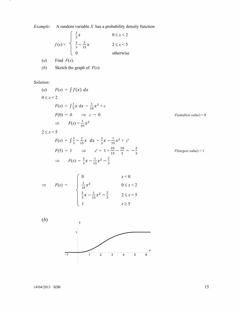
Example: A random variable X has a probability density function

0 ≤ x < 2

f (x) = 2 ≤ x < 5

0 otherwise

(a) Find F(x).

(b) Sketch the graph of F(x).

Solution:

(a) F(x) =  

0 ≤ x < 2

F(x) = 15   = + c

F(0) = 0 ⇒ c = 0 F(smallest value) = 0

⇒ F(x) =

2 ≤ x < 5

F(x) =     = + c′

F(5) = 1 ⇒ c′ = 1 + = F(largest value) = 1

⇒ F(x) = 23

0 x < 0

⇒ F(x) = 0 ≤ x < 2

23 2 ≤ x < 5

1 x ≥ 5

(b)

y = F(x)

−1 1 2 3 4 5 6

1

x

y

16 SDB 14/04/2013

Example: A dart is thrown at a dartboard of radius 25 cm. Let X be the distance from the centre to the point where the dart lands.

Assuming that the dart is equally likely to hit any point of the board find

(a) the cumulative probability density function for X.

(b) the probability density function for X.

Solution:

(a) F(x) = P(X < x) = P(the dart lands a distance of less than x from the centre)

=        radius         

=    .

⇒ F(x) = 0 x < 0

F(x) = 0 ≤ x ≤ 25

F(x) = 1 x > 25

(b)     = 2

625d xdx

⎛ ⎞⎜ ⎟⎝ ⎠

= 2625

x

⇒    

0 ≤ x ≤ 25

    0 otherwise

Expected mean and variance

Frequency, discrete and continuous probability distributions 

To change from a frequency distribution to a discrete probability distribution think of each probability

pi as Nf i ;

and to change from a discrete probability distribution think of the probability of x as the area of a narrow strip around x.

⇒ pi ≈ f (x) δx

then the formula for mean and variance etc are ‘the same’.

         δ x

f (x)

f(x)

x

14/04/2013 SDB 17

Frequency distribution

x1, x2, ... , xn

f1, f2, ... , fn

if N=∑

∑= ii fxN

m 1

∑ −= 222 1 mfxN

s ii

21 ( )ix mN

= −∑

Discrete probability distribution

x1, x2, ... , xn

p1, p2, ... , pn

∑ = 1ip

i ix pμ = ∑

222 μσ −=∑ ii px

2( )i ix pμ= −∑

Continuous probability distribution

-∞ < x < ∞

f(x)

     = 1

μ          

           

 

Mode, median & quartiles for a continuous random variable

Mode 

The mode is the ‘most popular’ and so will be at the greatest value of f (x) in the interval.

It is best to sketch a graph, using calculus to find the stationary points.

Remember that the mode might be at one end of the interval, not in the middle.

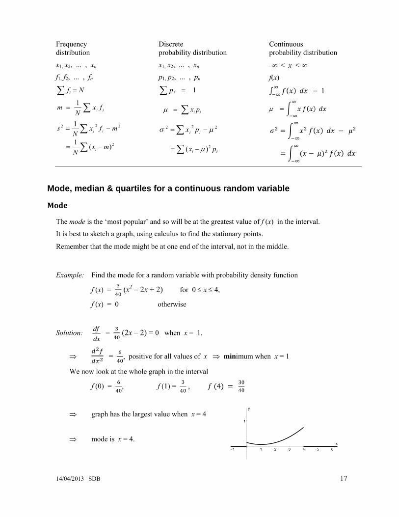
Example: Find the mode for a random variable with probability density function

f (x) = (x2 – 2x + 2) for 0 ≤ x ≤ 4,

f (x) = 0 otherwise

Solution: dxdf = (2x – 2) = 0 when x = 1.

⇒ = , positive for all values of x ⇒ minimum when x = 1

We now look at the whole graph in the interval

f (0) = , f (1) =  ,   4      3040

⇒ graph has the largest value when x = 4

⇒ mode is x = 4.

−1 1 2 3 4 5 6

1

x

y

18 SDB 14/04/2013

Median 

The median is the middle value and so the probability of being less than the median is ½ ;

so find M such that P(X < M) = .

⇒            .

Example: Find the median for a random variable with probability density function

f (x) = 2

20x

for 4 ≤ x ≤ 5,

f (x) = 0 otherwise.

Solution: The median M is given by 2120

4 2 =∫ dxx

M

⇒ = ⇒ + 5 =

⇒ M = 4

Quartiles 

Quartiles are found in the same way as the median.

P(X < Q1) = ⇒               .

P(X < Q3) = ⇒               .

14/04/2013 SDB 19

4 Continuous uniform (rectangular) distribution

Definition A continuous uniform distribution has constant probability density over a fixed interval.

Thus f (x) = αβ −

1 is the continuous uniform p.d.f. over the

interval [α, β ] and has a rectangular shape.

Median By symmetry the median is

2βα +

Mean and Variance The expected mean is E[X] = μ =

2βα + , which is the same as the median.

and the expected variance is Var[X] = σ 2 = 12

)( 2αβ − .

Proofs 

(a) Expected mean

E           1

     2  

                     

or by symmetry.

(b) Expected variance

Var       1

    2

      3     2       3       2  

      3      24

     212        12    

α

1

f (x)

xβ

20 SDB 14/04/2013

5 Normal Approximations

The normal approximation to the binomial distribution

Conditions for approximation 

For a binomial distribution B(n, p) we know that the mean is μ = np and the variance is σ 2 = npq.

If p is ‘near’ and if n is large, np > 10, then the normal distribution N(np, npq) can be used as an approximation to the binomial.

This is usually used when using the binomial would give awkward or tedious arithmetic.

Continuity correction 

A continuity correction must always be used when approximating the binomial with the normal (this means that 47 must be taken as 46⋅5 or 47⋅5 depending on the sense of the question).

Example: Find the probability of more than 20 sixes in 90 rolls of a fair die.

Solution: The exact distribution is binomial X ∼ B(90, ), where X is the number of sixes; but finding the exact probability would involve much tedious arithmetic.

Note that n is large, np = 15 > 10 so we can use the normal N(np, npq) as an approximation.

μ = np = 90 × = 15

σ 2 = npq = 90 × × = 12

⇒ μ = 15 and σ = √12⋅5 = 3⋅53553

So we use Y ∼ N (12, 12⋅5), where Y is the number of sixes

To find P(more than 20 sixes) we must include 21 but not 20 so, using a continuity correction, we find the area to the right of 20⋅5,

⇒ P(X > 20) = P(Y > 20⋅5)

= 1 – 20 5 153 53553⋅ −⎛ ⎞Φ ⎜ ⎟⋅⎝ ⎠

= 1 – Φ(1⋅5556)

= 1 – Φ(1⋅56) = 1 – 0⋅9406 = 0⋅0594 to 4 D.P. using tables

φ

x

15 20.5

14/04/2013 SDB 21

The normal approximation to the Poisson distribution

Conditions for approximation 

For a Poisson distribution PO(λ) we know that the mean is μ = λ and the variance is σ 2 = λ and

if n is large and λ > 10 then the normal distribution N(λ, λ) can be used as an approximation to the Poisson distribution PO(λ) .

This is usually used when using the Poisson would give awkward or tedious arithmetic.

Continuity correction 

As with the normal approximation to the binomial a continuity correction must always be used when approximating the Poisson with the normal.

Example: Cars arrive at a motorway filling station at a rate of 18 every quarter of an hour. Find the probability that at least 23 cars arrive in a quarter of an hour period.

Solution:

The exact distribution is Poisson X ∼ X ∼ PO(18), where X is the number of cars arriving in a hour period;

but finding the exact probability would involve much tedious arithmetic.

Note that n is large, λ = 18 > 10 so we can use the normal Y ∼ N(18, 18), where Y is the number of cars arriving in a ¼ hour period, as an approximation.

⇒ μ = 18 and σ = √18 = 4⋅2426

To find P(at least 23 cars) we must include 23 but not 22 so, using a continuity correction,

we find the area to the right of 22⋅5,

⇒ P(X ≥ 23) = P(Y > 22⋅5)

= 1 – 22 5 184 2426⋅ −⎛ ⎞Φ ⎜ ⎟⋅⎝ ⎠

= 1 – Φ(1⋅06)

= 1 – 0.8554 = 0.1446 to 4 D.P. using tables

18 22.5

x

22 SDB 14/04/2013

6 Populations and sampling Words and their meanings 

Population A collection of items.

Finite population A population is one in which each individual member can be given a number (a population might be so large that it is difficult or impossible to give each member a number – e.g. grains of sand on the beach).

Infinite population A population is one in which each individual member cannot be given a number.

Census An investigation in which every member of the population is evaluated.

Sampling unit A single member of the population which could be included in a sample .

Sampling frame A list of all sampling units, by name or number, from which samples are to be drawn (usually the whole population but not necessarily).

Sample A selection of sampling units from the sampling frame.

Simple random sample A simple random sample of size n, is one taken so that every possible sample of size n has an equal chance of being selected. The members of the sample are independent random variables, X1, X2, … , Xn , and each Xi has the same distribution as the population.

Sample survey An investigation using a sample.

Statistic A quantity calculated only from the data in the sample, using no unknown parameters (for example, μ and σ).

Sampling distribution of a statistic This is the set of all possible values of the statistic together with their individual probabilities; this is sometimes better described by giving the relevant probability density function.

14/04/2013 SDB 23

Advantages and disadvantages of taking a census 

Advantages Every member of the population is used. It is unbiased. It gives an accurate answer.

Disadvantages It takes a long time. It is costly. It is often difficult to ensure that the whole population is surveyed.

Advantages and disadvantages of sampling 

Advantages Sample will be representative if population large and well mixed. Usually cheaper. Essential if testing involves destruction (life of a light bulb, etc.). Data usually more easily available.

Disadvantages: Uncertainty, due to the natural variation – two samples are unlikely to give the same result. Uncertainty due to bias prevents the sample from giving a representative picture of the population and can occur through:

sampling from an incomplete sampling frame – e.g. using a telephone directory for people living in Bangkok

influence of subjective choice where supposedly random selection is affected by personal preferences - e.g. interviewing only the pretty women!

non-response where questionnaires about a particular mobile phone service is not answered by many who do not use that service

substituting convenient sampling units when those required are not readily available – e.g. visiting neighbours when sampling unit is out!

NOTE: Bias cannot be removed by increasing the size of the sample.

24 SDB 14/04/2013

Sampling distributions

To find the sampling distribution of the ******

We need all possible values of ******, together with their probabilities

Write down all possible samples together with their probabilities Calculate the value of ****** for each sample The sampling distribution of ****** is a list of all possible values of ****** together with their probabilities.

Example: A large bag contains £1 and £2 coins in the ratio 3 : 1.

A random sample of three coins is taken and their values X1, X2 and X3 are recorded.

Find the sampling distribution for the mean.

Solution: We must first find each sample, its mean and probability

Sample Mean Probability

(1, 1, 1) 1 (3/4)3 = 27/64

(1, 1, 2), (1, 2, 1), (2, 1, 1) 1 3 × (3/4)2 × (1/4) = 27/64

(1, 2, 2), (2, 1, 2), (2, 2, 1) 1 3 × (3/4) × (1/4)2 = 9/64

(2, 2, 2) 2 (1/4)3 = 1/64

and so the sampling distribution of the mean is

Mean 1 1 1 2

Probability 27/64 27/64 9/64 1/64

OR, you may be able to use a standard probability distribution

Example: A disease is present in a 23% of a population. A random sample of 30 people is taken and the number with the disease, D, is recorded. What is the sampling distribution of D?

Solution: The possible outcomes (values of D) are

D 0 1 … r … 30

with probabilities 0⋅7730 .0⋅7729× 0.23 … 30Cr ×0⋅7730–r×0.23r … 0.2330 

which we recognise as the Binomial distribution,

so the sampling distribution of D is D ~ B(30, 0.23)

14/04/2013 SDB 25

7 Hypothesis tests

Null hypothesis, H0 The hypothesis which is assumed to be correct unless shown otherwise.

Alternative hypothesis, H1 This is the conclusion that should be made if H0 is rejected

Hypothesis test A mathematical procedure to examine a value of a population parameter proposed by the null hypothesis, H0, compared to the alternative hypothesis, H1.

Test statistic This is the statistic (calculated from the sample) which is tested (in cumulative probability tables, or with the normal distribution etc.) as the last part of the test.

Critical region The range of values which would lead you to reject the null hypothesis, H0

Significance level The actual significance level is the probability of rejecting H0 when it is in fact true.

Null and alternative hypotheses, H0 and H1

Both null and alternative hypotheses must be stated in symbols only.

The null hypothesis, H0, is the ‘working hypothesis’, i.e. what you assume to be true for the purpose of the test.

The alternative hypothesis, H1, is what you conclude if you reject the null hypothesis: it also determines whether you use a one-tail or a two-tail test.

Your conclusion must be stated in full – both in statistical language and in the context of the question.

Critical region and significance level

From your observed result (test statistic) you decide whether to reject or not to reject the null hypothesis.

There will be an ‘acceptable’ region and if your observed result (test statistic) lies within this region then you will not reject the null hypothesis, H0.

The region outside this ‘acceptable’ region is called the critical region and if your observed result (test statistic) lies in this critical region then you will reject the null hypothesis, H0, and your conclusion will be based on the alternative hypothesis, H1.

If the significance level is 5% then the ‘acceptable region’ is 95% of all possible outcomes and the critical region is the remaining 5% of all possible outcomes.

(Note that ‘acceptable region’ is not official jargon so do not use it!!)

26 SDB 14/04/2013

One-tail and two-tail tests

The alternative hypothesis, H1, will indicate whether you should use a one-tail or a two-tail test.

For example:

H0: a = b

H1: a > b

You reject H0 only if b is significantly bigger than a. Thus you are only looking at one end of the population and a one-tail test is suitable.

H0: a = b

H1: a ≠ b

You reject H0 either if b is significantly bigger than a or if b is significantly less than a. Thus you are looking at both ends of the population and a two-tail test is suitable.

The points above are best illustrated by worked examples. Note that we always find the probability of the observed result or worse: this enables us to see easily whether the observed result lies in the critical region or not.

Worked examples (binomial, one­tail test)  

Example: A tetrahedral die (one with four faces! – each equally likely) is rolled 40 times and 6 ‘ones’ are observed. Is there any evidence at the 10% level that the probability of a score of l is less than a quarter?

Notice that the expected mean is 10 (= 40 × ), and we are really asking if the observed result (test statistic) 6 is ‘surprisingly low’.

Solution: H0: p = 0.25

H1: p < 0.25.

From H1 we see that a one-tail test is required, at 10% significance level.

If X is number of ‘ones’ then assuming binomial X ~ B(40, 0⋅25) and using the cumulative binomial tables

The test statistic (observed value) is X = 6

P(X ≤ 6 ‘ones’ in 40 rolls) = 0⋅0962 = 9⋅62% from tables

Since 9⋅62% < 10% the test statistic (observed result) lies in the critical region.

We reject H0 and conclude that

there is evidence to show that the probability of a score of 1 is lower than .

14/04/2013 SDB 27

Example: The probability that a footballer scores from a penalty is 0⋅8. In twenty penalties he scores only 13 times. Is there any evidence at the 5% level that the footballer is losing his form?

Solution: If X is the number of scores from 20 penalties, then X ∼ B (20, 0⋅8)

The cumulative binomial tables do not deal with p > 0.5 so we must ‘turn the problem round’ and consider Y, the number of misses in 20 penalties, where Y ∼ B (20, 0⋅2).

H0: p = 0⋅8 (or p = 0⋅2).

H1: p < 0⋅8 (or p > 0⋅2)

Observed value is X = 13

We consider the values X ≤ 13

⇒ X = 13 12 11 10 …

⇒ Y = 7 8 9 10 …

⇒ Y ≥ 7

Using the cumulative binomial tables, Y ∼ B (20, 0⋅2)

P(X ≤ 13) = P (Y ≥ 7)

= 1 – P (Y ≤ 6) = 1 – 0⋅9133 = 0⋅0867 = 8⋅67%

8⋅67% > 5% (significance level)

⇒ the test statistic (observed result) 7 is not significant (does not lie in the critical region),

Do not reject H0.

Conclude that there is evidence that the player has not lost his form, or that there is evidence that the probability of scoring from a penalty is still 0⋅8.

 

28 SDB 14/04/2013

Worked example (binomial test, two­tail critical region)  

Example: A tetrahedral die is manufactured with numbers 1, 2, 3 and 4 on its faces. The manufacturer claims that the die is fair.

All dice are tested by rolling 30 times and recording the number of times a ‘four’ is scored.

(a) Using a 5% significance level, find the critical region for a two-tailed test that the probability of a ‘four’ is . Find critical values which give a probability which is closest to 0⋅025.

(b) Find the actual significance level for this test.

(c) Explain how a die could pass the manufacturer’s test when it is in fact biased.

Solution:

(a) H0: p = 0⋅25.

H1: p ≠ 0⋅25 the die is not fair if there are too many or too few ‘fours’

From H1 we can see that a two-tailed test is needed, significance level 2⋅5% at each end.

Let X be number of ‘four’s in 30 rolls then we assume a binomial distribution, X ~ B(30, 0⋅25).

We shall reject the hypothesis if the observed result lies in either half of the critical region each half having a significance level of 2⋅5%;

For a two tail test, find the values of X which give a probability closest to 2⋅5% at each end.

Using cumulative binomial tables for X ∼ B (30, 0⋅25):

for the lower critical value from tables

P(X ≤ 2) = 0⋅0106 (2.5% – 1.06% = 1.44%) P(X ≤ 3) = 0⋅0374 (3.74% – 2.5% = 1.24%)

X ≤ 3 gives the value closest to 2⋅5%, so X = 3 is lower critical value

and for the higher critical value from tables

P(X ≥ 13) = 1– P(X ≤ 12) = 1 – 0.9784 = 0.0216 (2.5% – 2.16% = 0.34%)

P(X ≥ 12) = 1– P(X ≤ 11) = 1 – 0.9493 = 5.07% (5.07% – 2.5% = 2.57%)

X ≥ 13 gives the value closest to 2⋅5%, so X = 13 is higher critical value

Thus the critical region is X ≤ 3 or X ≥ 13.

(b) The actual significance level is 0⋅0374 + 0⋅0216 = 0⋅0590 = 5⋅90%. to 3 S.F.

(c) The die could still be biased in favour of, or against, one of the other numbers.

14/04/2013 SDB 29

Worked example (Poisson)  

Example: Cars usually arrive at a motorway filling station at a rate of 3 per minute. On a Tuesday morning cars are observed to arrive at the filling station at a rate of 5 per minute. Is there any evidence at the 10% level that this is an unusually busy morning?

Solution: H0: λ = 3

H1: λ > 3 unusually busy would mean that λ would increase

From H1 we see that a one-tail test is needed, significance level 10%.

It seems sensible to assume that the numbers of cars arriving per minute is independent, uniform and single so a Poisson distribution is suitable.

Let X be the number of cars arriving per minute, then X ~ PO(3)

The test statistic (observed value) is X = 5

P(X ≥ 5) = 1 – P(X ≤ 4) = 1 – 0⋅8153 = 0⋅1847 = 18⋅47% > 10% using tables

which is not significant at the 10% level. Do not reject H0.

Conclude that there is evidence that Tuesday morning is not unusually busy,

or there is evidence that cars are still arriving at a rate of 3 cars per minute.

Worked example (Poisson, critical region)  

Example: Over a long period in the production of glass rods the mean number of flaws per 5 metres is 4. A length of 10 metres is to be examined. Find the critical region to show that the machine is producing too many flaws at the 5% level.

Find the lowest value which gives a probability of less than 5%.

Solution:

H0: λ = 8 flaws occur uniformly, so if mean per 5 metres is 4, then mean per 10 metres is 8

H1: λ > 8 machine producing too many flaws would mean that λ would increase

We can see from H1 that we need a one- tail test, significance level 5%.

For a one tail test, find the first value of X for which the probability is less than 5% It seems sensible to assume that the number of flaws per 10 metre lengths is independent, uniform and single so a Poisson distribution is suitable.

X ~ PO(8) where X is the number of flaws in a 10 metre length

P(X ≥ 13) = 1 – P(X ≤ 12) = 1 – 0⋅9362 = 0⋅0638 = 6⋅38% > 5% from tables

P(X ≥ 14) = 1 – P(X ≤ 13) = 1 – 0⋅9784 = 0⋅0216 = 2⋅16% < 5%

⇒ X = 14 is the smallest value for which the probability is less than 5%

⇒ the critical region is X ≥ 14.

30 SDB 14/04/2013

Hypothesis testing using approximations.

Example: With current drug treatment, 9% of cases of a certain disease result in total recovery. A new treatment is tried out on a random sample of 100 patients, and it is found that 16 cases result in total recovery. Does this indicate that the new treatment is better at a 5% level of significance?

Solution: Let X be the number of cases resulting in total recovery.

H0: p = 0.09

H1: p > 0.09

X ~ B(100, 0.09), which is not in the tables and is awkward arithmetic, so we use an approximation.

λ or μ = np = 100 × 0.09 = 9 < 10,

n large and p small ⇒ we should use the Poisson approximation Y ~ PO(9)

The test statistic is Y = 16.

We want P (X ≥ 16) ≈ P (Y ≥ 16)

= 1 – P (Y ≤ 15) = 1 – 0⋅9780 = 0⋅0220 < 5% from tables

⇒ the test statistic is significant at 5%

⇒ Reject H0.

Conclude that there is some evidence that the proportion of cases of total recovery has increased from 0.09 under the new treatment.

14/04/2013 SDB 31

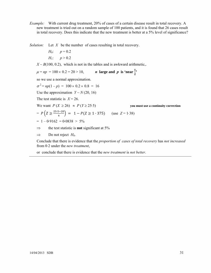
Example: With current drug treatment, 20% of cases of a certain disease result in total recovery. A new treatment is tried out on a random sample of 100 patients, and it is found that 26 cases result in total recovery. Does this indicate that the new treatment is better at a 5% level of significance?

Solution: Let X be the number of cases resulting in total recovery.

H0: p = 0.2

H1: p > 0.2

X ~ B(100, 0.2), which is not in the tables and is awkward arithmetic,.

μ = np = 100 × 0.2 = 20 > 10, n large and p is ‘near ’

so we use a normal approximation.

σ 2 = np(1 – p) = 100 × 0.2 × 0.8 = 16

Use the approximation Y ~ N (20, 16)

The test statistic is X = 26.

We want P (X ≥ 26) ≈ P (Y ≥ 25⋅5) you must use a continuity correction

= ·     1 1 · 375 (use Z = 1⋅38)

= 1 – 0⋅9162 = 0⋅0838 > 5%

⇒ the test statistic is not significant at 5%

⇒ Do not reject H0.

Conclude that there is evidence that the proportion of cases of total recovery has not increased from 0⋅2 under the new treatment,

or conclude that there is evidence that the new treatment is not better.

32 SDB 14/04/2013

8 Context questions and answers

Accuracy You are required to give your answers to an appropriate degree of accuracy.

There is no hard and fast rule for this, but the following guidelines should never let you down.

1. If stated in the question give the required degree of accuracy. 2. When using a calculator, give 3 S.F.

unless finding Sxx,, Sxy etc. in which case you can give more figures – you should use all figures when finding the PMCC or the regression line coefficients.

3. Sometimes it is appropriate to give a mean to 1 or 2 D.P. rather than 3 S.F. 4. When using the tables and doing simple calculations (which do not need a calculator), you

should give 4 D.P.

General vocabulary Question 1

Define a statistic.

Answer

A number calculated from known observations (from a sample) – no unknown parameters.

Question 2

Explain what you understand by the statistic Y.

Answer

A statistic is a calculation from the values in the sample, 1 2, ,... nX X X that does not contain any unknown parameters.

Question 3

Define the critical region of a test statistic.

Answer

The set of values of the test statistic for which the null hypothesis is rejected in a hypothesis test.

14/04/2013 SDB 33

Question 4

Explain what you understand by

(a) a population,

(b) a statistic.

A researcher took a sample of 100 voters from a certain town and asked them who they would vote for in an election. The proportion who said they would vote for Dr Smith was 35%.

(c) State the population and the statistic in this case.

(d) Explain what you understand by the sampling distribution of this statistic.

Answer

(a) A population is collection of all items

(b) A calculation from the sample which contains no unknown quantities/parameters.

(c) The population is ‘voters in the town’. The statistic is ‘percentage/proportion voting for Dr Smith’.

(d) List of all possible samples (of size 100) of those voting for Dr Smith together with the probability of each sample.

Skew Question 1

Explain why the distribution is negatively skewed.

Answer

Mean < median < mode (⇒ negative skew): give values.

Question 2

Given that the median is 1.40, describe the skewness of the distribution. Give a reason for your answer.

Answer

Positive skew

Q3 – Q2 > Q2 – Q1 give values (box plot with Q1, Q2, Q3 values marked on – optional)

Or mode = 1 and mode < median = give value.

34 SDB 14/04/2013

Binomial distribution

Question 1

A company claims that a quarter of the bolts sent to them are faulty. To test this claim the number of faulty bolts in a random sample of 50 is recorded. Give two reasons why a binomial distribution may be a suitable model for the number of faulty bolts in the sample

Answer Two from 2 outcomes / faulty or not faulty / success or fail.

A constant probability of a faulty bolt Trials are independent.

Fixed number of trials (fixed n). Poisson distribution

Question 2

State two conditions under which a Poisson distribution is a suitable model for X.

Answer

Misprints are random / independent, occur singly in space and at a constant rate

Question 3

An estate agent sells properties at a mean rate of 7 per week.

Suggest a suitable model to represent the number of properties sold in a randomly chosen week. Give two reasons to support your model.

Answer

PO(7) Sales occur independently/randomly, singly, at a constant rate (context needed once)

Question 4

A call centre agent handles telephone calls at a rate of 18 per hour.

(a) Give two reasons to support the use of a Poisson distribution as a suitable model for the number of calls per hour handled by the agent.

Answer

Calls occur singly any two of the 3

Calls occur at a constant rate

Calls occur independently or randomly.

14/04/2013 SDB 35

Question 5

Explain how the answers from part (c) support the choice of a Poisson distribution as a model.

Answer

For a Poisson model , Mean = Variance ; For these data 3.69≈3.73 ⇒ Poisson

Approximations to Poisson and Binomial

Question 1

Giving a justification for your choice, use a suitable approximation to estimate the probability that there are exactly 5 defective articles.

Answer

For the binomial distribution X ~ B(200 , 0⋅02) n is large, p is small so use the Poisson approximation Y ~ PO (np) = Po (4).

Question 2

(a) State the condition under which the normal distribution may be used as an approximation to the Poisson distribution.

(b) Explain why a continuity correction must be incorporated when using the normal distribution as an approximation to the Poisson distribution.

Answer

(a) λ > 10 or large (use μ instead of λ is OK).

(b) The Poisson distribution is discrete and the normal distribution is continuous.

Question 3

Write down the conditions under which the Poisson distribution may be used as an approximation to the Binomial distribution.

Answer

If X ~ B(n,p) and

n is large, n > 50

p is small, p < 0⋅2 (or q = 1 – p is small) but I would not worry too much about the 0⋅2 and the 50.

then X can be approximated by Po(np)

36 SDB 14/04/2013

Question 4

Write down two conditions for X ~ B (n, p) to be approximated by a normal distribution

Y ~ N (μ, σ 2).

Answer

If X ~ B(n,p) and

n is large or n > 10 or np > 5 or nq >5

p is close to 0.5 or nq > 5 and np > 5

then X can be approximated by Y ~ N(np, npq).

Sampling

Question 1

Explain what you understand by

(a) a sampling unit.

(b) a sampling frame.

(c) a sampling distribution.

Answer

(a) Individual member or element of the population or sampling frame.

(b) A list of all sampling units or all the population.

(c) All possible samples are chosen from a population; the values of a statistic together with the associated probabilities is a sampling distribution.

Question 2

Before introducing a new rule, the secretary of a golf club decided to find out how members might react to this rule.

(a) Explain why the secretary decided to take a random sample of club members rather than ask all the members.

(b) Suggest a suitable sampling frame.

(c) Identify the sampling units.

Answer

(a) Saves time / cheaper / easier or

a census/asking all members takes a long time or is expensive or difficult to carry out

(b) List, register or database of all club members/golfers

(c) Club member(s)

14/04/2013 SDB 37

Question 3

Explain what you understand by the sampling distribution of Y.

Answer

The probability distribution of Y, or the distribution of all possible values of Y together with their probabilities.

38 SDB 14/04/2013

Index accuracy, 32

binomial distribution, 4, 12, 20, 28 mean, 7 normal approximation, 20 poisson approximation, 11 probabilities, 5 variance, 7

binomial theorem, 4 binomial coefficients, 4

census, 22

combinations, 3 nCr, 4 properties, 3

continuity correction normal approx to binomial, 20 normal approx to poisson, 21

continuous uniform distribution, 19 mean, 19 median, 19 variance, 19

critical region, 25, 28, 29

cumulative probability density function, 14

factorials, 3

hypothesis test, 25 alternative, 25 alternative hypothesis, 25 binomial, critical region, 28 binomial, two-tail, 28 null, 25 null hypothesis, 25 one-tail, 26 poisson, critical region, 29

poisson, one tail, 29 two-tail, 26 using normal approximation, 30

pascal’s triangle, 4

poisson distribution, 8 conditions, 8 mean, 10 normal approximation, 21 probabilities, 9 variance, 10

population, 22 finite, 22

probability density function conditions, 13 mean, 16 median, 17 mode, 17 quartiles, 17 variance, 16

sample, 22 advantages, 23 disadvantages, 23 simple random, 22

sampling distribution, 22 worked example, 24

sampling frame, 22

sampling unit, 22

significance level, 25

statistic, 22 test statistic, 25