statistical models for natural sounds
TRANSCRIPT

Statistical models
for natural sounds
Richard E. Turner
M.A., M.Sci., Natural Sciences (Physics), University of Cambridge, UK (2003)
Gatsby Computational Neuroscience Unit
University College London
7 Queen Square
London, WC1N 3AR, United Kingdom
THESIS
Submitted for the degree of
Doctor of Philosophy, University of London
2010

2
I, Richard E. Turner, confirm that the work presented in this thesis is my own. Where
information has been derived from other sources, I confirm that this has been indicated
in the thesis.

3
Abstract
It is important to understand the rich structure of natural sounds in order to solve im-
portant tasks, like automatic speech recognition, and to understand auditory processing
in the brain. This thesis takes a step in this direction by characterising the statistics of
simple natural sounds. We focus on the statistics because perception often appears to
depend on them, rather than on the raw waveform. For example the perception of au-
ditory textures, like running water, wind, fire and rain, depends on summary-statistics,
like the rate of falling rain droplets, rather than on the exact details of the physical
source.
In order to analyse the statistics of sounds accurately it is necessary to improve a
number of traditional signal processing methods, including those for amplitude demod-
ulation, time-frequency analysis, and sub-band demodulation. These estimation tasks
are ill-posed and therefore it is natural to treat them as Bayesian inference problems.
The new probabilistic versions of these methods have several advantages. For exam-
ple, they perform more accurately on natural signals and are more robust to noise,
they can also fill-in missing sections of data, and provide error-bars. Furthermore,
free-parameters can be learned from the signal. Using these new algorithms we demon-
strate that the energy, sparsity, modulation depth and modulation time-scale in each
sub-band of a signal are critical statistics, together with the dependencies between the
sub-band modulators. In order to validate this claim, a model containing co-modulated
coloured noise carriers is shown to be capable of generating a range of realistic sounding
auditory textures.
Finally, we explored the connection between the statistics of natural sounds and per-
ception. We demonstrate that inference in the model for auditory textures qualitatively
replicates the primitive grouping rules that listeners use to understand simple acoustic
scenes. This suggests that the auditory system is optimised for the statistics of natural
sounds.

4
Acknowledgments
A simple recipe for doing research is to surround yourself with smart, approachable,
and provocative people. I have been extremely fortunate that the Gatsby Unit contains
many people of this ilk.
First and foremost, Maneesh Sahani has been an excellent supervisor. Generous with
his time and able to provide both high-level inspiration and also detailed technical help,
he has allowed me great freedom to work on a range of problems of my choice. I am
extremely grateful for his wisdom and his kindness.
The enduring quality of the Gatsby Unit owes much to its director, Peter Dayan, who is
a consummate researcher and deft politician. May the numerous seminars and daily tea-
talks continue forever. I am enormously grateful to the Gatsby charitable foundation
for funding my research and providing travel money. I’d also like to extend a special
thanks to Rachel Howes, whose administrative help often extended beyond the call of
duty.
The training during my PhD benefited greatly from collaborating closely with Pietro
Berkes, who taught me a great deal and with whom it is great fun to work. Thanks also
for the countless nuggets of advice and help offered by Iain Murray and Kai Krueger. I
consider myself very fortunate to have studied for my PhD at the same time as Misha
Ahrens and Louise Whiteley, who give excellent advice and who are close friends:
Thanks to you both.
I would also like to thank David Mackay for his friendship, guidance (both scientific and
career related), and not least for nudging me towards Gatsby in the first place. Thanks
also to Roy Patterson for kindling my interest in natural sounds and the auditory
system.
Next to my examiners, John Shawe-Taylor and Neil Lawrence, who were extremely
constructive and whose feedback improved a number of sections of the thesis markedly.
They caught a number of errors, and of course any that remain are entirely my own.
Finally, I would also like to thank my family — Mum, Helen, Jude and Luce — for
all their support and patience down the years. Most importantly, I’d like to thank my
Dad who inspired me to study science, who encouraged me to go into research, and
who was the first person I used to turn to for advice and support. I hope, were he still
alive, that he would have been proud of this thesis.

Contents
Front matter
Abstract . . . . . . . . . . . . . . . . . . . . . . . . . . . . . . . . . . . . . . . 3
Acknowledgments . . . . . . . . . . . . . . . . . . . . . . . . . . . . . . . . . . 4
Contents . . . . . . . . . . . . . . . . . . . . . . . . . . . . . . . . . . . . . . . 5
List of figures . . . . . . . . . . . . . . . . . . . . . . . . . . . . . . . . . . . . 10
1 Why build probabilistic models for natural sounds? 12
1.1 The importance of prior information . . . . . . . . . . . . . . . . . . . . 12
1.2 Prior information as statistical information . . . . . . . . . . . . . . . . 13
1.3 Probabilistic approaches to machine and human audition . . . . . . . . 14
1.4 Thesis Themes . . . . . . . . . . . . . . . . . . . . . . . . . . . . . . . . 15
1.4.1 Unpacking the statistics of sounds . . . . . . . . . . . . . . . . . 16
1.4.2 Probabilising signal processing methods . . . . . . . . . . . . . . 16
1.4.3 Human audition as inference . . . . . . . . . . . . . . . . . . . . 17
1.5 Outline of the thesis . . . . . . . . . . . . . . . . . . . . . . . . . . . . . 17
2 Background 19
2.1 Signal processing methods for demodulation . . . . . . . . . . . . . . . 19
2.1.1 Simple Demodulation Algorithms . . . . . . . . . . . . . . . . . 20
2.1.2 Sub-band demodulation . . . . . . . . . . . . . . . . . . . . . . . 23
2.1.3 Sinusoidal modelling . . . . . . . . . . . . . . . . . . . . . . . . 25
2.1.4 Computational Auditory Scene Analysis . . . . . . . . . . . . . 26
2.1.5 Applications of demodulation . . . . . . . . . . . . . . . . . . . 26
2.1.5.1 Vocoders . . . . . . . . . . . . . . . . . . . . . . . . . . 27
2.1.5.2 Cochlear Implants . . . . . . . . . . . . . . . . . . . . . 28
2.1.6 Summary . . . . . . . . . . . . . . . . . . . . . . . . . . . . . . . 29
2.2 Statistics of natural sounds . . . . . . . . . . . . . . . . . . . . . . . . . 30
2.2.1 Model-Free Statistics . . . . . . . . . . . . . . . . . . . . . . . . 30
2.2.2 Model-Based Statistics . . . . . . . . . . . . . . . . . . . . . . . . 31
2.2.2.1 Simple Probabilistic Models . . . . . . . . . . . . . . . 31
2.2.2.2 Modelling Residual Dependencies . . . . . . . . . . . . 33
2.2.2.3 Gaussian Scale Mixtures and Amplitude Modulation . 35
2.2.2.4 Modelling Temporal Dependencies . . . . . . . . . . . 36

CONTENTS 6
2.2.3 Summary . . . . . . . . . . . . . . . . . . . . . . . . . . . . . . . 37
2.3 Biological evidence for modulation processing . . . . . . . . . . . . . . . 38
2.4 Conclusion . . . . . . . . . . . . . . . . . . . . . . . . . . . . . . . . . . 40
3 Probabilistic Amplitude Demodulation 41
3.1 Simple Probabilistic Amplitude Demodulation . . . . . . . . . . . . . . 43
3.1.1 The forward model . . . . . . . . . . . . . . . . . . . . . . . . . . 43
3.1.2 Relationship with existing models . . . . . . . . . . . . . . . . . 45
3.1.3 Inference . . . . . . . . . . . . . . . . . . . . . . . . . . . . . . . 46
3.1.4 Results and Improvements to S-PAD . . . . . . . . . . . . . . . . 47
3.2 Gaussian Process Probabilistic Amplitude Demodulation . . . . . . . . 49
3.2.1 Forward Model . . . . . . . . . . . . . . . . . . . . . . . . . . . . 49
3.2.2 Efficient inference using circular data . . . . . . . . . . . . . . . 50
3.2.3 MAP Inference . . . . . . . . . . . . . . . . . . . . . . . . . . . . 52
3.2.3.1 The SLP method as a heuristic inference scheme . . . 54
3.2.3.2 Testing MAP inference . . . . . . . . . . . . . . . . . . 55
3.2.4 Error-bars and Laplace’s Approximation . . . . . . . . . . . . . 57
3.2.4.1 Experiments and practical considerations . . . . . . . . 59
3.2.5 Parameter Learning . . . . . . . . . . . . . . . . . . . . . . . . . 61
3.2.5.1 Learning parameters from the marginal data . . . . . . 61
3.2.5.2 Learning the time-scale using Laplace’s Approximation 63
3.2.6 Summary of GP-PAD . . . . . . . . . . . . . . . . . . . . . . . . 65
3.3 Improving the model: SP-PAD . . . . . . . . . . . . . . . . . . . . . . . 66
3.3.1 Bayesian Spectrum Analysis . . . . . . . . . . . . . . . . . . . . 66
3.3.2 Bayesian Modulation Spectrum Analysis . . . . . . . . . . . . . 68
3.3.2.1 Error-bars . . . . . . . . . . . . . . . . . . . . . . . . . 70
3.3.3 Summary . . . . . . . . . . . . . . . . . . . . . . . . . . . . . . . 71
3.4 Missing and noisy data . . . . . . . . . . . . . . . . . . . . . . . . . . . 71
3.5 Results . . . . . . . . . . . . . . . . . . . . . . . . . . . . . . . . . . . . 72
3.5.1 Deterministic modulation . . . . . . . . . . . . . . . . . . . . . . 73
3.5.2 Estimator Axioms . . . . . . . . . . . . . . . . . . . . . . . . . . 74
3.5.3 Denoising . . . . . . . . . . . . . . . . . . . . . . . . . . . . . . . 80
3.5.4 Natural Data . . . . . . . . . . . . . . . . . . . . . . . . . . . . . 81
3.5.4.1 Sub-band demodulation . . . . . . . . . . . . . . . . . . 82
3.5.4.2 Filling in missing data . . . . . . . . . . . . . . . . . . 85
3.5.5 Summary Statistics . . . . . . . . . . . . . . . . . . . . . . . . . 86
3.5.5.1 Modulation Depth . . . . . . . . . . . . . . . . . . . . 88
3.5.5.2 Modulation time-scale . . . . . . . . . . . . . . . . . . . 89
3.5.5.3 Cross-channel modulation dependencies . . . . . . . . . 89
3.6 Summary . . . . . . . . . . . . . . . . . . . . . . . . . . . . . . . . . . . 91
4 Modulation Cascades 93

CONTENTS 7
4.1 Modulation Cascade Forward Model . . . . . . . . . . . . . . . . . . . . 94
4.1.1 Relationship to PAD . . . . . . . . . . . . . . . . . . . . . . . . . 94
4.2 MAP Inference . . . . . . . . . . . . . . . . . . . . . . . . . . . . . . . . 95
4.2.1 Initialisation . . . . . . . . . . . . . . . . . . . . . . . . . . . . . 95
4.3 Learning in the cascade model . . . . . . . . . . . . . . . . . . . . . . . 96
4.4 Automatic determination of the number of modulators . . . . . . . . . 97
4.4.1 Testing inference and learning . . . . . . . . . . . . . . . . . . . 98
4.5 Results . . . . . . . . . . . . . . . . . . . . . . . . . . . . . . . . . . . . . 98
4.6 Summary . . . . . . . . . . . . . . . . . . . . . . . . . . . . . . . . . . . 99
5 Cross-frequency Probabilistic Amplitude Demodulation 102
5.1 A simple analysis of cross-channel modulation . . . . . . . . . . . . . . 103
5.1.1 Dimensionality Reduction; PCA . . . . . . . . . . . . . . . . . . 103
5.1.2 Rotation; SFA . . . . . . . . . . . . . . . . . . . . . . . . . . . . 103
5.1.3 Chapter Outline . . . . . . . . . . . . . . . . . . . . . . . . . . . 104
5.2 Probabilistic Time Frequency Representations . . . . . . . . . . . . . . 106
5.2.1 Traditional Time-Frequency Representations . . . . . . . . . . . 106
5.2.2 Probabilistic Time-Frequency Representations . . . . . . . . . . 108
5.2.2.1 General Framework . . . . . . . . . . . . . . . . . . . . 109
5.2.2.2 Tractable Time Frequency Models . . . . . . . . . . . . 113
5.2.2.3 AR(2) Filter Bank . . . . . . . . . . . . . . . . . . . . 113
5.2.2.4 Probabilistic Phasors . . . . . . . . . . . . . . . . . . . 115
5.2.3 Conclusion . . . . . . . . . . . . . . . . . . . . . . . . . . . . . . 121
5.3 Multivariate Probabilistic Amplitude Demodulation . . . . . . . . . . . 123
5.3.1 The forward model . . . . . . . . . . . . . . . . . . . . . . . . . 123
5.3.1.1 Relationship to other models . . . . . . . . . . . . . . . 124
5.3.2 Inference . . . . . . . . . . . . . . . . . . . . . . . . . . . . . . . 126
5.3.2.1 Relationship to other inference schemes . . . . . . . . . 127
5.3.3 Learning . . . . . . . . . . . . . . . . . . . . . . . . . . . . . . . . 129
5.3.4 Testing Learning and Inference in M-PAD(ARc) . . . . . . . . . 131
5.3.5 Results . . . . . . . . . . . . . . . . . . . . . . . . . . . . . . . . 132
5.3.5.1 Generation of synthetic sounds . . . . . . . . . . . . . 133
5.3.5.2 Filling in missing data . . . . . . . . . . . . . . . . . . 137
5.4 Conclusions and Future Directions . . . . . . . . . . . . . . . . . . . . . 139
6 Primitive Auditory Scene Analysis as Inference 141
6.1 Primitive Auditory Scene Analysis . . . . . . . . . . . . . . . . . . . . . 142
6.1.1 Proximity . . . . . . . . . . . . . . . . . . . . . . . . . . . . . . 142
6.1.2 Good-continuation . . . . . . . . . . . . . . . . . . . . . . . . . . 143
6.1.3 Common-fate . . . . . . . . . . . . . . . . . . . . . . . . . . . . 144
6.1.3.1 Common Amplitude Modulation . . . . . . . . . . . . 144
6.1.3.2 Common Frequency Modulation . . . . . . . . . . . . . 144

CONTENTS 8
6.1.4 The old plus new heuristic . . . . . . . . . . . . . . . . . . . . . 145
6.1.5 Harmonicity . . . . . . . . . . . . . . . . . . . . . . . . . . . . . 145
6.1.6 Closure . . . . . . . . . . . . . . . . . . . . . . . . . . . . . . . . 146
6.1.7 Comodulation Masking Release . . . . . . . . . . . . . . . . . . 147
6.1.8 The perception of phase . . . . . . . . . . . . . . . . . . . . . . 148
6.1.9 Complications to the grouping picture . . . . . . . . . . . . . . . 149
6.2 Computational Model . . . . . . . . . . . . . . . . . . . . . . . . . . . . 149
6.2.1 The forward model and inference . . . . . . . . . . . . . . . . . . 150
6.2.2 Constraints from phase and Frequency Modulation perception . 151
6.2.3 Proximity as inference . . . . . . . . . . . . . . . . . . . . . . . . 152
6.2.4 Good continuation . . . . . . . . . . . . . . . . . . . . . . . . . . 153
6.2.5 Common Amplitude Modulation . . . . . . . . . . . . . . . . . . 154
6.2.6 Closure and the continuity illusion . . . . . . . . . . . . . . . . . 155
6.2.7 CMR . . . . . . . . . . . . . . . . . . . . . . . . . . . . . . . . . 156
6.2.8 Old plus new heuristic . . . . . . . . . . . . . . . . . . . . . . . . 158
6.3 Conclusions and future directions . . . . . . . . . . . . . . . . . . . . . . 159
7 Conclusion 162
7.1 Probabilising signal processing methods . . . . . . . . . . . . . . . . . . 163
7.2 Unpacking the statistics of natural sounds . . . . . . . . . . . . . . . . . 164
7.3 Probabilistic Auditory Scene Analysis . . . . . . . . . . . . . . . . . . . 165
A Circulant Matrices 167
A.1 Circulant Matrices . . . . . . . . . . . . . . . . . . . . . . . . . . . . . . 167
A.2 Stationary Covariance Matrices on regularly sampled points . . . . . . 169
B Weight space view of stationary Gaussian Processes 171
C Auto-regressive processes 173
C.1 Preliminaries . . . . . . . . . . . . . . . . . . . . . . . . . . . . . . . . . 173
C.2 Stationarity . . . . . . . . . . . . . . . . . . . . . . . . . . . . . . . . . 174
C.3 Auto-correlation . . . . . . . . . . . . . . . . . . . . . . . . . . . . . . . 176
C.4 Power Spectrum . . . . . . . . . . . . . . . . . . . . . . . . . . . . . . . 176
C.5 From spectra to AR parameters . . . . . . . . . . . . . . . . . . . . . . 179
D Demodulation as a convex optimisation problem 182
D.1 Probabilistic convex demodulation . . . . . . . . . . . . . . . . . . . . . 182
D.2 Estimator Axioms . . . . . . . . . . . . . . . . . . . . . . . . . . . . . . 183
D.3 Comparison of the approaches . . . . . . . . . . . . . . . . . . . . . . . . 185
E List of Acronyms 187
F Summary of Models 189
F.1 Models for Probabilistic Amplitude Demodulation . . . . . . . . . . . . 189

CONTENTS 9
F.1.1 Simple Probabilistic Amplitude Demodulation . . . . . . . . . . 189
F.1.2 Gaussian Process Probabilistic Amplitude Demodulation (1) . . 190
F.1.3 Gaussian Process Probabilistic Amplitude Demodulation (2) . . 191
F.1.4 Student-t Process Probabilistic Amplitude Demodulation . . . . 192
F.1.5 Modulation Cascade Process . . . . . . . . . . . . . . . . . . . . 193
F.2 Models for Probabilistic Time Frequency Analysis . . . . . . . . . . . . 194
F.2.1 Second order Auto-Regressive Process (AR(2)) Filter bank . . . 195
F.2.2 Bayesian Spectrum Estimation . . . . . . . . . . . . . . . . . . . 195
F.2.3 The Probabilistic Phase Vocoder . . . . . . . . . . . . . . . . . . 196
F.3 Models for Probabilistic Primitive Auditory Scene Analysis . . . . . . . 198
F.3.1 Multivariate Probabilistic Amplitude Demodulation (1) . . . . . 198
F.3.2 Multivariate Probabilistic Amplitude Demodulation (2) . . . . . 199
F.3.3 Kalman Smoothing Recursions . . . . . . . . . . . . . . . . . . . 200
F.3.4 Forward Filter Backward Sample Algorithm . . . . . . . . . . . 201
References 202

List of figures
1.1 Introduction to speech production . . . . . . . . . . . . . . . . . . . . . 13
2.1 A typical signal model for AM . . . . . . . . . . . . . . . . . . . . . . . 21
2.2 Graphical models for sparse coding and the GSM. . . . . . . . . . . . . 35
3.1 Traditional and probabilistic amplitude demodulation. . . . . . . . . . . 42
3.2 A sample from S-PAD. . . . . . . . . . . . . . . . . . . . . . . . . . . . . 44
3.3 S-PAD applied to a speech sound . . . . . . . . . . . . . . . . . . . . . . 47
3.4 GP-PAD envelope non-linearity. . . . . . . . . . . . . . . . . . . . . . . . 50
3.5 A sample from GP-PAD . . . . . . . . . . . . . . . . . . . . . . . . . . . 51
3.6 Graphical model for GP-PAD . . . . . . . . . . . . . . . . . . . . . . . . 52
3.7 Testing MAP inference. . . . . . . . . . . . . . . . . . . . . . . . . . . . 56
3.8 Eigen-spectra for exact Laplace. . . . . . . . . . . . . . . . . . . . . . . . 58
3.9 Laplace’s Approximation for GP-PAD . . . . . . . . . . . . . . . . . . . 60
3.10 Parameter learning tests. . . . . . . . . . . . . . . . . . . . . . . . . . . 64
3.11 Learning time-scales in GP-PAD . . . . . . . . . . . . . . . . . . . . . . 65
3.12 Demodulation of the S100S175/S11S15 signal . . . . . . . . . . . . . . . 75
3.13 Demodulation of the WN/S11S15 signal . . . . . . . . . . . . . . . . . . 76
3.14 Summary of deterministic demodulation . . . . . . . . . . . . . . . . . . 77
3.15 Demodulation of a pure tone . . . . . . . . . . . . . . . . . . . . . . . . 78
3.16 Demodulation of a carrier and an envelope . . . . . . . . . . . . . . . . . 79
3.17 Spectra of carriers and modulators derived from filtered speech. . . . . . 80
3.18 Demodulation of noisy synthetic data. . . . . . . . . . . . . . . . . . . . 81
3.19 Demodulating noisy speech data. . . . . . . . . . . . . . . . . . . . . . . 82
3.20 GP-PAD applied to spoken sentences. . . . . . . . . . . . . . . . . . . . 83
3.21 GP-PAD applied to bird-song. . . . . . . . . . . . . . . . . . . . . . . . . 84
3.22 GP-PAD applied to the sound of a deep stream. . . . . . . . . . . . . . 84
3.23 GP-PAD applied to a jungle scene. . . . . . . . . . . . . . . . . . . . . . 85
3.24 GP-PAD and the Hilbert method applied to speech sub-bands. . . . . . 86
3.25 Filter bank demodulation . . . . . . . . . . . . . . . . . . . . . . . . . . 87
3.26 Filter bank demodulation . . . . . . . . . . . . . . . . . . . . . . . . . . 87
3.27 Filling in missing envelopes of speech . . . . . . . . . . . . . . . . . . . . 88
3.28 Summary modulation statistics . . . . . . . . . . . . . . . . . . . . . . . 90

LIST OF FIGURES 11
3.29 Correlation of sub-band modulation . . . . . . . . . . . . . . . . . . . . 91
4.1 Demodulation Cascade via recursive demodulation . . . . . . . . . . . . 94
4.2 Testing Demodulation Cascade Inference . . . . . . . . . . . . . . . . . . 99
4.3 Demodulation Cascade representation of speech . . . . . . . . . . . . . . 100
4.4 Demodulation Cascade representation of a jungle sound . . . . . . . . . 101
5.1 PCA on speech modulators . . . . . . . . . . . . . . . . . . . . . . . . . 104
5.2 PCA and SFA on speech modulators . . . . . . . . . . . . . . . . . . . . 105
5.3 Resynthesis from a filter bank. . . . . . . . . . . . . . . . . . . . . . . . 108
5.4 Filter banks and Probabilistic Time Frequency Representations . . . . . 112
5.5 AR(2) spectra . . . . . . . . . . . . . . . . . . . . . . . . . . . . . . . . . 115
5.6 Comparison of the gammatone and AR(2) filter banks. . . . . . . . . . . 116
5.7 Probabilistic filter bank and STFT coefficients. . . . . . . . . . . . . . . 118
5.8 Comparison of the gammatone and Probabilistic Spectrogram. . . . . . 120
5.9 Uncertainty relation for the probabilistic spectrogram. . . . . . . . . . . 122
5.10 Testing learning in M-PAD . . . . . . . . . . . . . . . . . . . . . . . . . 132
5.11 M-PAD applied to speech . . . . . . . . . . . . . . . . . . . . . . . . . . 136
5.12 Typical results for filling in missing sections of speech. . . . . . . . . . . 138
5.13 A summary of the results of filling in missing sections of speech. . . . . 139
6.1 Grouping by proximity as inference . . . . . . . . . . . . . . . . . . . . . 153
6.2 Grouping by good continuation as inference . . . . . . . . . . . . . . . . 154
6.3 Grouping by common AM as inference . . . . . . . . . . . . . . . . . . . 155
6.4 The continuity illusion as inference . . . . . . . . . . . . . . . . . . . . . 157
6.5 Comodulation Masking Release as inference . . . . . . . . . . . . . . . . 158
6.6 The old plus new heuristic as inference . . . . . . . . . . . . . . . . . . . 160
C.1 Samples from an AR(2) process . . . . . . . . . . . . . . . . . . . . . . . 173
C.2 Domain of stationary AR(2) processes . . . . . . . . . . . . . . . . . . . 175
C.3 The autocorrelation of an AR(2) process . . . . . . . . . . . . . . . . . . 177
C.4 The spectrum of an AR(2) process . . . . . . . . . . . . . . . . . . . . . 178
C.5 AR(2) spectra . . . . . . . . . . . . . . . . . . . . . . . . . . . . . . . . . 178
C.6 From AR(2) parameters to filter properties. . . . . . . . . . . . . . . . . 179
C.7 Approximating spectra using and AR(2) process . . . . . . . . . . . . . 181
D.1 Comparison of GP-PAD and convex amplitude demodulation. . . . . . . 186

Chapter 1
Why build probabilistic models
for natural sounds?
1.1 The importance of prior information
Natural sounds are complex, richly structured signals. For monophonic signals (i.e. those
which are not stereo) all of this rich structure is laid out in the temporal dimension.
Speech, for example, contains structure at the level of the formants (the milli-second
time-scale), pitch (tens of milli-seconds), phonemes (hundreds of milli-seconds) and
sentences (seconds) (see figure 1.1).
It is important to characterise the rich structure in speech and other natural sounds, as
it is a prerequisite for solving a range of tasks in machine-audition, and also for under-
standing the way the auditory system processes sounds. For example, a prototypical
machine-audition task is to remove unwanted noise from a signal (Wang and Brown,
2006). So called denoising tasks require the true signal to be distinguished from the
noise, and this is only possible using prior knowledge of the structure of the signal and
of the noise. One of the tasks that this thesis focuses on is demodulation which involves
representing a signal as the product of a quickly varying carrier and a slowly varying,
positive envelope. Again this is only possible using prior information like the difference
in the time-scale of the carrier and envelope. The reliance on prior information becomes
greater as the complexity of the task increases. Perhaps the most complex task of all is
to replicate on a computer the remarkable ability of humans to analyse complex acous-
tic scenes and to break them into their constituent parts. This is called Computational
Auditory Scene Analysis (CASA) (Wang and Brown, 2006) and it is far from being a
solved problem, but the approaches that have been developed thus far all rely on prior
knowledge of natural sounds. For instance, many sounds contain harmonic sections
and so time-frequency representations are a ubiquitous starting point (Cohen, 1994).
The fact that machine audition relies heavily on prior knowledge can be traced back to

Prior information as statistical information 13
Figure 1.1: Speech is one of the most richly structured natural sounds. It isproduced by pulses of air which enter the throat and mouth through the vocalfolds and excite resonances called formants. The formant frequencies depend onthe shape of the vocal tract (which includes the throat, mouth and nasal cavities),but they tend to be on the order of 1000Hz. Typically, the shape of the vocal tractis fixed for period of about 100ms, which gives rise to the basic units of speechcalled phonemes out of which words are built. The vocal folds control the natureof the pulses of air entering the cavities. In one mode, a build up of air fromthe lungs causes the folds to open and snap shut in a periodic fashion every tenmilli-seconds or so. This gives rise to a periodic excitation which is heard as thepitch of sounds. Phonemes produced in this way, like the vowel sounds, are calledvoiced phonemes (e.g the /a/ sound in ‘hard’). In another mode, the airflow isturbulant giving rise to unvoiced phonemes like the fricatives e.g. the sound ‘f’.
the fact that the problems it tries to solve are often ill-posed. Denoising, for instance,
involves estimating both the noise component and the true signal, at each time-step of
a one-dimensional input. Similarly, demodulation involves estimating both the carrier
and the envelope at each time-step. CASA involves estimation of an even larger number
of variables per time-step, including the number and location of the component sources,
the contribution from each, and so on. It is well known that ill-posed problems cannot
be solved without recourse to prior information (Jaynes, 2003). This conclusion is
quite general and applies to human auditory scene analysis as well as to computational
approaches.
1.2 Prior information as statistical information
We have established that prior information is essential to machine and human audition,
but it is not immediately clear what form this information should take. We argue that
natural sounds can only be characterised through their statistics (McDermott et al.,
2009) and so this prior information should be statistical. For instance, no two “rain”

Probabilistic approaches to machine and human audition 14
sounds are identical, because the precise arrangement of falling water droplets is never
repeated. Consequently, the perceptual similarity of two rain sounds cannot be derived
from a direct comparison of their waveforms. Instead the similarity must be derived at
the level of the statistics of the sounds, that is the aspects of the waveform which relate
to the rate of falling rain-drops, the distribution of droplet sizes, and so on. It seems
natural that acoustic textures (Strobl et al., 2006; Lu et al., 2004), like rain, wind,
running-water, fire, crowd noise etc., are amenable to a statistical description, because
their physics can be described statistically. However, this perspective is also useful for
other sounds. For instance, a wide range of different stimuli are perceived as a particular
vowel type, everything from simple synthetic sounds with sinusoids at the formant
frequencies (Rosner and Pickering, 1994), through to the huge diversity of natural vowel
sounds (Peterson and Barney, 1952; Hillenbrand et al., 1995). Even whispered vowels,
in which the vocal tract is excited by aspirated noise, are recognisable. The implication
is that the percept of vowel type, like the perception of auditory textures, does not
depend on the precise details of the waveform, but on summary statistics.
1.3 Probabilistic approaches to machine and human au-
dition
We have argued above that machine and human audition are often faced with ill-posed
problems which require prior information to be solved. What is more, we have ar-
gued that the form of relevant prior information is often statistical. From a theoretical
perspective, what is needed is a calculus for reasoning with this prior information in
order to solve problems like denoising, demodulation, and CASA, and also to under-
stand how the brain might compute using prior information. In fact the calculus of
Bayesian inference has been identified as the optimal method for reasoning with in-
complete or uncertain information (Cox, 2002; Jaynes, 2003; MacKay, 2003). However,
technical difficulties, like those associated with encoding meaningful prior information,
have meant that that most approaches to machine audition have largely ignored the
Bayesian approach, instead opting for heuristic methods. One of the contributions of
this thesis are a number of technical advances that enable Bayesian methods to be
applied to a range of machine audition tasks. The approach begins by specifying a
generative model which is a description of how the signal (y) is produced from latent
variables (x). For instance, in demodulation the latent variables will be the unknown
carrier and envelope, whilst in CASA, the latent variables might represent the various
sources that could be present in a scene, like a rain texture or a vowel sound. As the
relationship between the signal and the latent variables is statistical, it is encoded prob-
abilistically in the emission distribution, p(y|x, θ). So, this distribution might capture
the fact that a rain-source can produce a range of different signals, whose long-time
statistics are fixed. The generative model also includes a description of the latent vari-

Thesis Themes 15
ables, p(x|θ), called the prior. For demodulation this would be a description of the
statistics of the fast carrier and slow modulator, whilst for CASA this would include a
description of which sources tend to be present in a scene.
The generative model gets its name from the fact that it is a recipe for producing
synthetic sounds in which the latent variables are first drawn probabilistically from
the prior, and then the sound is generated from them using the emission distribution.
Generating synthetic data in this way provides a useful method for validating the
modelling assumptions. Importantly, the generative model can be turned on its head
in order to infer the latent variables from the scene, using Bayes’ theorem,
p(x|y, θ) =p(x|θ)p(y|x, θ)
p(y|θ) . (1.1)
In the case where the latent variables are carriers and envelopes, this posterior distri-
bution describes the probability of the carrier and envelope given the signal, which is
the solution to the demodulation problem. And when the latent variables are sources,
this posterior distribution describes the probability of occurrence of the sources, given
the observed signal; this is auditory scene analysis.
The generative model includes parameters (θ), which control the relationship between
the latent variables and the waveform, as well as the prior. Often it is not a simple
matter to set these parameters by hand, but fortunately they can be learned from the
statistics of sound, for example, by maximising the likelihood of the parameters,
L(θ) = p(y|θ) =∑
x′
p(y|x′, θ)p(x′|θ). (1.2)
In practice, the likelihood is a difficult quantity to form as it involves a summation over
the latent variables which is often intractable. For this reason approximation methods
are often required for learning and also for inference (as the likelihood of the parameters
normalises the posterior). In fact, much of the hard labour in the generative approach
is concerned with finding accurate, but tractable approximation schemes.
In the next section, we describe how probabilistic methods are used in this thesis.
1.4 Thesis Themes
The content of this thesis lies at the interface of the fields of machine-audition, signal-
processing, and computational neuroscience. This leads to three main themes and in
each of these generative models play an important role. The first theme is to determine
the basic statistical regularities in sounds which make them sound natural. In order to
tease apart these statistics it is necessary to develop new signal processing methods.
This gives rise to the second theme of the thesis which is to develop these new methods

Thesis Themes 16
by building probabilistic analogues to a range of existing signal processing methods,
including methods for demodulation and time-frequency analysis. The probabilistic
approaches to demodulation and time-frequency analysis can be combined to form a
model which captures many of the low level statistics of natural sounds. Interestingly,
inference in this model replicates the basic rules which listeners appear to use to under-
stand simple stimuli. This idea, that primitive auditory scene analysis can be explained
as inference in a generative model, is the third theme. These three themes will now be
explained in more detail.
1.4.1 Unpacking the statistics of sounds
Natural auditory scenes are hierarchically organised as they contain sources (like a
person talking), which are composed of component parts (like vowels and consonants),
that can be further broken down into structural primitives (like amplitude modulated
harmonic complexes and noise) (Bregman, 1994; Darwin and Carlyon, 1995). This hi-
erarchical structure means that the statistics of sounds are very complicated. From the
generative perspective, it means that a model of natural scenes must also be hierarchi-
cal, with each level containing a potentially large number of latent variables. This is
a very challenging problem, but a sensible first step is to concentrate on just the first
level of this hierarchy. That is, modelling the structural primitives out of which other
sounds can be composed. This is the goal of this thesis.
We argue that the structural primitives of natural sounds are quickly varying carriers
that undergo slow modulation. Together, the statistics of the carriers, which model
the fine-structure of sounds, and the modulation, which model patterns of spectral-
temporal power, are sufficient to capture the statistics of simple sounds, like basic
auditory textures.
The importance of the modulation and fine-structure of sounds has long been recognised
and many signal processing methods have been developed to represent these quantities.
Therefore, these existing approaches are used as a starting point in the development of
new models. By analysing the aspects of the statistics of sounds which these models
fail to capture, they can then be generalised. This approach is described in the next
section.
1.4.2 Probabilising signal processing methods
The process of probabilising a signal processing method (Roweis, 2004) begins by identi-
fying a generative model for which the existing method can be viewed as approximating
inference. Having identified a suitable generative model, a more principled inference
scheme can be developed. The new methods often provide a superior solution, but be-
cause they are more complex (e.g. non-linear and/or recurrent) they are usually more

Outline of the thesis 17
computationally intensive. However, the new probabilistic signal processing methods
have several other benefits. First, articulation of a forward model allows the assump-
tions behind the methods to be critiqued and improved. Generally speaking, whilst
a generative model might be simple to understand and develop intuitions from, the
associated exact-inference algorithm will often appear much more complex in compar-
ison. The generative model thus provides a useful theoretical perspective from which
improvements to complicated inference schemes can be made fairly simply. Two other
benefits of the generative approach are the ability to return uncertainties in the esti-
mated quantities, and the great simplicity of resynthesis. Resynthesis is simple because
it involves passing the (possibly modified) latent variables through the emission distri-
bution. This is much more complicated in traditional approaches as they are focussed
purely on analysis without a complementary synthesis algorithm. A consequence of
the simplicity of resynthesis and an ability to handle uncertainties, is that filling in
missing sections of data and denoising are both simple to handle using the generative
approach. A final advantage of the probabilistic approach is that free parameters in
the models can be learned e.g. by maximum-likelihood estimation. This avoids the ad
hoc hand-tuning of parameters which are a feature of many existing methods.
1.4.3 Human audition as inference
This thesis develops a model for primitive auditory scene synthesis, and so inference
in this model can be thought of as primitive auditory scene analysis. There is a large
literature in auditory psychophysics which describes primitive auditory scene analysis,
as well as a related literature that describes the perception of modulation. We will
show that many of these findings are consistent with the idea that the auditory system
is inferring the modulation and fine-structure in sounds.
1.5 Outline of the thesis
The thesis begins in chapter 2 by reviewing three different literatures that all point to
the fact that modulation is a key statistic of natural sounds. In the signal processing
literature demodulation algorithms are established as key components in solutions for
audio-coding, audio-manipulation, speech-recognition, and cochlear implants. In the
field of natural scene statistics, amplitude modulation is yet to be modelled explicitly,
but we show that it reveals itself in the residual statistical dependencies that current
models fail to capture. In the auditory neuroscience literature, there is strong evidence
from psychophysics and electrophysiology indicating that the auditory system listens
attentively to Amplitude Modulation (AM).
The third chapter of the thesis develops models for probabilistic amplitude demodu-
lation. Key to these models are three new theoretical developments; fast circularised

Outline of the thesis 18
Gaussian Processes (which enable quick inference), Lanczos-Laplace error-bar estima-
tion (for approximating the uncertainty in estimated modulators), and Bayesian Mod-
ulation Spectrum Estimation (for inferring the spectrum of the modulation). Proba-
bilistic Amplitude Demodulation methods out-perform traditional ways of estimating
AM in natural signals according to a variety of metrics. For instance, when a carrier
extracted by Probabilistic Amplitude Demodulation (PAD) is itself demodulated, the
this results in an (almost) constant modulator and carrier which is a rescaled version
of the signal. This is a critical consistency test which indicates that all of the modula-
tor information has been removed from the carrier i.e. it is demodulated. Traditional
methods fail this test catastrophically. More generally, PAD extends the range of de-
modulation tasks to problems involving noisy signals or missing data. The new methods
are used to characterise the statistics of AM in natural sounds. We find that that nat-
ural sounds are characterised by AM which is correlated both over long time-scales and
across multiple frequency bands.
Another of the conclusions of chapter 3 is that the modulators in natural sounds often
contain multiple time-scales. One of the ways in which this reveals itself is in the fact
that modulators recovered from natural sounds are themselves modulated. Therefore
chapter 4 is concerned with modelling this structure and the approach is to recursively
demodulate a signal, its envelope, the envelope that results from that and so on. This
new representation is called a Demodulation Cascade.
A second conclusion from chapter 3 is that the modulators in different sub-bands of a
natural sound are often strongly correlated. Chapter 5 develops probabilistic models
which capture these dependencies. The first step is to develop a probabilistic time-
frequency representation which will be used to model the carriers in natural sounds.
Probabilistic time-frequency representations have several advantages over traditional
representations affording simple resynthesis procedures, methods for parameter learning
(i.e. learning the filter properties) and handling uncertainty (e.g. in missing data and
denoising tasks). The second step is combine the model for the carriers with one for the
envelopes of sounds. The resulting model can be trained on natural sounds and then
used to synthesise a range of realistic sounding simple auditory textures like running
water, wind, fire and rain. Moreover, it is also applied to missing data tasks where it
out-performs models which do not model the modulation content of sounds.
The generative model developed in chapter 5 can be interpreted as a model for primi-
tive auditory scene synthesis because it can generate simple scenes involving auditory
textures. Turning this on its head, inference in these models amount to primitive au-
ditory scene analysis. Chapter 6 shows that a large number of psychophysical results
can be qualitatively modelled as inference in this manner.

Chapter 2
Background
We will argue in this chapter that several different literatures point to the fact that
modulation is a key statistical regularity in natural sounds. The chapter starts by
reviewing various signal processing methods for estimating the modulation content of a
signal (section 2.1). This is a logical place to begin, as modulation can only be precisely
defined by describing the method by which it is estimated. The chapter then goes on to
describe how modulation is critical for many important machine-audition tasks, such
as audio-compression, audio-manipulation, audio-retrieval, speech-recognition, and also
in the audio-processing in cochlear implants (section 2.1.5). The implication is that a
key signature of natural sounds is their modulation content. The second part of this
chapter reviews work that has characterised the statistical structure of natural sounds
(section 2.2). We will argue that there is growing evidence that amplitude modulation
is a pervasive form of statistical regularity which has been largely over-looked. The
third part of this chapter considers the biological evidence for modulation processing
and concludes that there is a large body of electrophysiological and psychophysical work
which indicates that the auditory system listens attentively to amplitude modulation
in natural sounds, both across different frequency channels and at different time-scales
(section 2.3).
2.1 Signal processing methods for demodulation
Demodulation is the process by which a signal (yt) is decomposed into a product of
slowly varying, positive envelope (at), and a quickly varying (positive and negative)
carrier (ct), that is, yt = atct. This problem is ill-posed (Loughlin and Tacer, 1996)
as it involves representing the one-dimensional signal at each time-step in terms of
two quantities; the carrier and envelope. Consequently, there are an infinity of ways
to demodulate a signal (one for each positive envelope, a1:T ). Ill-posed problems can
only be solved using prior information, and we will later argue that this means the
inferential approach to demodulation is a natural one, not least because it makes this

Signal processing methods for demodulation 20
prior knowledge explicit. In contrast, current approaches to demodulation are not
probabilistic, and the prior knowledge used to realise the representation often remains
tacit.
2.1.1 Simple Demodulation Algorithms
This section will discuss a number of methods for demodulating signals. Before specific
algorithms are covered, we will briefly review some of the theoretical ideas upon which
these methods are founded. Interestingly, there are connections with the probabilistic
approach.
Most successful demodulation schemes are either derived from a signal model or from
a set of estimator-axioms1. A signal model (Schimmel, 2007) is a description of the
assumptions made about the signal and it is essentially a form of generative model,
although it is not probabilistic. Instead, the signal model specifies a list of deterministic
constraints, which are often chosen in the hope of making the problem well-posed. For
instance, the fact that the modulator is slow and the carrier is quick is often translated
into the assumption that the modulator contains only low-frequency energy up to some
cut-off, and that the carrier only contains energy at frequencies larger than this cut-off.
If the bandwidth of the carrier is also assumed to be small, this renders the problem
well-posed. This is the signal model for AM radio and it is illustrated in figure 2.1.
Whilst the signal model is concerned with synthesis, the estimator-axioms are concerned
with analysis. Essentially, they are a set of desirable properties that inference should
have, for instance that demodulation should be covariant with respect to scale changes
in the input signal,
y′t = αyt =⇒ a′t = αaat and c′t = αcct. (2.1)
Or that both the estimated carrier and envelope should be bounded. The observation
that several traditional demodulation methods, developed using signal models, violated
these seemingly unrestrictive axioms led to the development of methods explicitly de-
signed to satisfy sets of estimator-axioms. One disadvantage of this approach is that
it is not clear what prior knowledge about the signal is being assumed. Interestingly,
these concerns do not arise in the probabilistic version of amplitude demodulation, as
equivalents to the estimator-axioms arise automatically from manipulation of the signal
(or generative) model using the rules of probability.
We will now describe some of the main approaches to demodulation with reference to
the signal model or estimator axioms from which they are derived. The first method
for demodulation considered here was originally designed for AM radio signals (see
figure 2.1 for the signal model). A simple two step method to demodulate such signals
1This is our term for a collection of properties authors have stipulated that a demodulation methodshould possess.

Signal processing methods for demodulation 21
0en
velo
pe
0
carr
ier
0 0.02 0.04 0.06 0.08 0.1
0
data
time /s
0
0
−1000 −500 0 500 10000
frequency /Hz
×
=
⊗
=
Figure 2.1: A typical signal model for AM shown in the time domain (left handpanels) and the frequency domain (right hand panels). The modulator (red, toprow) is positive and slowly varying. The carrier (blue, middle row) is quicklyvarying and real valued. Here it is a band-pass Gaussian noise process with afairly narrow bandwidth. The spectrum of the modulated signal is formed fromthe convolution of the modulator spectrum and the carrier spectrum, which resultsin side-lobes. For AM radio signals the carriers are pure tones, ct = sin(ωRFt+Φ),and the modulator a band-pass target-signal which has been shifted to ensurepositivity. Squaring the signal moves modulator energy to low frequencies, y2
t =12a2
t (1 − cos(2(ωRFt+ Φ))), which is the basis of the SLP method.
is: First, square the signal to move energy from the modulator to low frequencies2.
Second, low-pass filter the result in order to pick off the energy from the modulator.
This method, called the SLP method (Libbey, 1994), is exact provided the carrier is
a pure sinusoid with a frequency greater than the highest frequency component in the
envelope, and the low-pass filter cut-off lies between the modulator and carrier energy.
However, this signal model is very restrictive. When the SLP method is applied to
more complex signals, a reasonable modulator can be extracted by judicious choice of
the low-pass filter cut-off. However, the recovered carrier is often poor. This is because
the envelope often becomes small, or even zero, in regions where the signal is non-zero
and this causes the associated carrier to be very large, even unbounded.
The failure of the SLP method to return bounded carrier estimates, and the need to
set the low-pass filter, motivate the development of new demodulation method which is
guaranteed to return a bounded carrier and which requires no hand-tuning. One way
to derive such a method begins by representing the signal as the real part of a complex
signal, and defining the magnitude of this complex-signal as the amplitude and the
2In actual fact many non-linear functions of the signal have this effect.

Signal processing methods for demodulation 22
sinusoidal component as the carrier, yt = ℜ (at exp(iφt)). This ensures the carrier
is bounded by construction. The question is how to specify the missing imaginary
component of the complex signal and one approach is to specify a set of estimator
axioms which enable it to be pinned down (Vakman, 1996). Vakman used the following
axioms;
1. A small change in the signal should result in a small change in the envelope.
2. The carrier must be invariant to amplitude scaling of the signal.
3. A single sinusoid must be decomposed into a constant envelope and a constant
frequency.
Vakman shows that the Hilbert transform,
H(y)(t) = p.v.
∫ ∞
−∞dτ
1
πτy(t− τ), (2.2)
where p.v. is the principal value of the integral, is the only way of specifying an imag-
inary signal which satisfies these axioms. This demodulation method will henceforth
be called the Hilbert Envelope (HE) method (Gabor, 1946). As a by-product, the
HE method provides a way of estimating the instantaneous frequency of a signal,
φt = φt − φt−1, and therefore the Frequency Modulation (FM) content.
There are, however, several problems with the HE method. Practically, the HE method
performs well when the carriers in a signal are simple sinusoids. However, when the
carriers have a more complicated form, the HE can provide a poor estimate of the
signal envelope, depending on the application. For example, if the signal is a pair of
harmonically related sinusoids that undergo slow modulation,
yt = at (sin(ωt) + sin(2ωt)) , (2.3)
the HE will contain a contribution at the fundamental frequency, ω, no matter how
slow the amplitude is. The tendency of the HE to contain high-frequency content
when applied to signals with structured carriers can be problematic (see figure 3.1).
For instance it means that the HEs extracted from natural sounds will often contain
pitch information which it is often desirable to separate from the modulation content
(Sell and Slaney, submitted). The HE has theoretical problems too. For example, a
bounded signal can give rise to a HE which is unbounded (Loughlin and Tacer, 1996).
Furthermore, the Hilbert carrier is not limited to the same frequency region as the
signal, which causes reconstruction problems (Dugundji 1958 and see section 2.1.2).
These observations motivate the introduction of additional estimator axioms and the
development of other demodulation schemes. In fact there are now a plethora of al-
ternatives; Mandelstram’s method, Shekels method, the Teager-Kaiser algorithm and
so on, for a review see Kvedalen 2003 and Potamianos et al. 1994. However, Vakman
argues that despite the limitations of the HE method, the performance of alternative

Signal processing methods for demodulation 23
algorithms is still inferior (Vakman, 1996). Similarly, there are also many schemes for
computing the instantaneous frequency of a signal, but once again it is argued that
the analytic signal is still the benchmark method (Girolami and Vakman, 2002). For
this reason, the SLP and HE methods will be used for the purposes of comparison in
this thesis. This completes the review of basic demodulation methods. In the following
sections these methods will be used as modules in procedures for deriving more complex
representations of signals.
2.1.2 Sub-band demodulation
The basic signal model described in the previous section is not rich enough to capture
the structure of natural sounds, like speech, and therefore efforts have been made to
generalise it (Schimmel, 2007). One of the limitations is that sounds like the vowels of
speech contain multiple carriers and so a natural extension is to describe a signal as a
sum of amplitude-modulated carriers,
yt =
D∑
d=1
cd,tad,t. (2.4)
In order to make this signal model well-posed each carrier-modulator pair (cd,tad,t) is
typically constrained to be band-pass and non-overlapping. Usually this is achieved by
constraining the carriers to be high-frequency, narrow-band processes and the envelopes
to be sufficiently slow. A heuristic scheme for estimating the carriers and envelopes
then begins by filtering the signal with a band-pass filter bank,
yFBd,t =
∑
t′
Wd,t−t′yt′ . (2.5)
Although the exact frequency composition of the signal is unknown before the filter-
ing step, the simplifying assumption is made that it is possible to choose the pass-
band of the filters a priori so that each filter covers a single modulator-carrier pair.
Filtering therefore isolates one component of the mixture and this implies that the
modulators can be recovered by independently demodulating each sub-band. The
most common method for sub-band demodulation method is to use the HE method
(Flanagan and Golden, 1966; Kinnunen, 2006; Thompson and Atlas, 2003). Sub-band
demodulation via the HE method is often performed using filters which are frequency-
shifted versions of one another so that, Wd,t = Wt cos(ω(c)d t), Flanagan (1980) shows
that this procedure derives modulators which are equal to the magnitude of the Short

Signal processing methods for demodulation 24
Time Fourier Transform (STFT) of the incoming sound3,
ySTFTd,t =
∑
t′
exp(−iωdt′)Wt′yt′ . (2.6)
The magnitude of the STFT is also called the spectrogram. This connection between
sub-band demodulation and the spectrogram is important as it has been argued that
the spectrogram, or features derived from the spectrogram, are of great utility for tasks
like speech recognition (Ellis, 2008) and music retrieval (Orio, 2006). Therefore, it
appears that the sub-band modulation structure is a critical statistic for recognising
sounds like speech (Drullman et al., 1994) and music.
Despite the ubiquity of the HE method, there are several potential problems with
its application to band-limited signals. The first problem is that the spectrum of the
estimated carrier signal generally exceeds the bandwidth of the signal (Dugundji, 1958).
This is surprising as it can be shown that important quantities like the square of the
envelope, a2t , and the square of the envelope times the phase, φta
2t are band-limited to
the same range as the signal (Flanagan, 1980).
Intuitively speaking, the fact that the carriers recovered using the HE method are not
band limited means that they often contain some of the envelope information in the
signal. This can result in artefacts when the carriers are used in resynthesis. For
example, Smith et al. (2002) synthesise auditory chimera using the sub-band HE infor-
mation from one sound and the Hilbert carrier information from another. They report
70% to 90% correct recognition performance for chimeric sounds which contain one-
or two-band speech fine structure and noise envelopes. This result was interpreted as
indicating that fine-structure cues were of major importance in this task. However,
this finding must be taken with a pinch of salt because the broad-band Hilbert carriers
actually contain much of the narrow-band envelope information (Zeng et al., 2004). In
a related procedure, Drullman et al. (1994) low-pass filter the sub-band HE informa-
tion in speech sounds, and resynthesise using the filtered envelopes and the original
carrier. The goal being to determine listener’s sensitivity to different time-scales of
modulation. However, because the Hilbert carriers are not band-limited, Drullman’s
processing technique creates modulation filtered signals that still contain rich enve-
lope information much beyond the cut-off frequency of the low-pass modulation filter
(Ghitza, 2001; Schimmel, 2007). The message is that resynthesis using the HE method
is fraught with difficulty.
A second problem with the application of the HE method to sub-band demodulation is
that it assumes that the input signal is equivalent to a simple product of a carrier and
modulator, whereas it is actually a filtered product. This filtering step is important
because, whereas a modulated signal is conjugate-symmetric (see the lower right-hand
3For a derivation of this result and a wider discussion of time-frequency representations, seesection 5.2.1

Signal processing methods for demodulation 25
panel of figure 2.1), a filtered product is not. This causes problems for the HE method
(Atlas et al., 2004).
Atlas et al. (2004) suggest a potential resolution to the two problems above. The pro-
posed solution to the first problem is to place an explicit constraint on the carrier
frequency content so that it is band-limited. The proposed solution to the second
problem is more radical and that is to sacrifice the idea of a positive, real-valued mod-
ulator and instead to relax this condition so that the modulator can be complex. This
enables signals with non-symmetric side-bands to be modelled. Due to this departure
from conventional ideas of amplitude demodulation, these methods cannot be compared
directly to traditional methods in terms of the estimated modulators, instead compar-
ison is more involved having to proceed through performance on a task like speech
reconstruction. It is therefore not completely clear how successful this new approach
is.
An alternative resolution to the problems inherent in sub-band demodulation is to
regard the whole process — both the filtering stage and the demodulation stage — as
an inference problem (see chapter 5). This involves writing down a generative model
for the signal in terms of a sum of narrow-band carriers which undergo slow amplitude
modulation. Estimation then proceeds using the rules of probability to invert the
model, and automatically respects the prior constraints on the envelopes and carriers,
like their spectral content. Furthermore, resynthesis using modified carrier and envelope
variables is simple, and free from heuristics.
2.1.3 Sinusoidal modelling
In the last section we described how to represent a sound in terms of a sum of am-
plitude modulated carriers by demodulating the output of a filter bank using the HE
method. For typical sounds, the number of sinusoids that are active at any one time
is much smaller than the total number of channels in the filter bank and this means
these representations are often inefficient. For this reason, sinusoidal modelling pro-
vides a decomposition of sounds in terms of a variable number of AM-FM modulated
sinusoids. These decompositions are realised using a number of heuristics. For exam-
ple, the McAulay Quatieri (MQ) algorithm (McAulay and Quatieri, 1986, 1995) begins
by isolating peaks in the spectrogram, and then joins up these peaks through time in
order to form smooth tracks that represent the time-varying envelopes and instanta-
neous frequencies of the sinusoidal components. Often there are more spectral peaks
at one time-step than another, and so heuristics are introduced that control the birth
and death of the tracks. The McAulay Quatieri algorithm is a fairly successful method
for modelling the voiced components of speech, but it fares less well for the unvoiced
components as these are not simple to explain in terms of a small number of AM-FM
sinusoids. One improvement is to model the MQ residual with a noise process, which is

Signal processing methods for demodulation 26
called spectral modelling synthesis (Serra and Smith, 1990). Another option is to aug-
ment the model with a modulated coloured-noise component, and to use heuristics to
estimate the modulation. The increase in the number of variables makes the estimation
problem more difficult, and so it is common to restrict the sinusoidal component to be
harmonic in order to increase the power of the estimate. This is called the Harmonic
Plus Noise model (Stylianou et al., 1995; Stylianou, 2005).
An insight into the possible upper-level of performance of sinusoidal models can be
gleaned from the fact that it is possible for an expert, with considerable time and ef-
fort, to correct the decompositions recovered by sinusoidal modelling so that speech can
be reasonably well approximated by just three AM-FM sinusoids (Remez et al., 1981;
Davis, 2007). However, although the heuristic schemes for computing sinusoidal decom-
positions continue to grow in complexity (Sainath, 2005), algorithms which replicate
this level of performance appear to be a very long way off. One of the problems is that it
is not clear how the ballooning number of heuristics should trade-off with one another.
In principle, this could be aided by probabilistic versions (e.g. see Parra and Jain 2001
for one attempt), but the probabilistic model has to be complex and this introduces
other problems. chapter 6 addresses these issues and provides new probabilistic models
for these tasks.
2.1.4 Computational Auditory Scene Analysis
Sinusoidal models, described in the previous section, began by decomposing sounds
into a sum of independent AM-FM sinusoids, but as they have been developed a wider
range of features have been incorporated into the analysis, like harmonic stacks and
noise busts. In this regard these analyses are becoming similar to to full-blown CASA
systems (Wang and Brown, 2006), which have a more general goal of grouping together
spectro-temporal energy arising from common sources. Typically, CASA systems also
rely on a large number of heuristics to perform this grouping with associated hand-tuned
parameters. An automatic method for determining heuristics and tuning the large
number of parameters would therefore be extremely useful. Probabilistic approaches
to CASA have been proposed as a potential solution (Ellis, 2006), but such models are
still in their infancy. Progress has been slow, mainly because the complexity of the
problem calls for large, richly structured models, in which inference and learning are
extremely challenging. One potential starting point, which is adopted in this thesis in
chapter 6, is to focus on just the first stage of auditory scene analysis called primitive
auditory scene analysis (Bregman, 1994).
2.1.5 Applications of demodulation
Demodulation algorithms have many important applications in machine-audition. It
has already been noted that the spectrogram – an estimate of the modulation in the

Signal processing methods for demodulation 27
different sub-bands of a signal – is of great importance in speech-recognition, and music
retrieval (Ellis, 2008; Orio, 2006). A number of related modulation based features have
also been used in these applications (Hermansky et al., 1991, 1992; Kingsbury et al.,
1998; Kanedera et al., 1998; Tyagi et al., 2003). In this section we describe two other
important applications of demodulation algorithms in speech-vocoders and cochlear
implants. On the face of it these applications are very different; speech vocoders are
efficient methods for coding speech which are useful for telecommunications (Spanias,
1994), whilst cochlear implants are artificial methods for transducing sounds recorded
at the outer ear into electrical activity in the auditory nerve, thereby by-passing a
damaged cochlea. Nevertheless, both applications share a common architecture, the
heart of which is a filter bank in which each of the channels has been demodulated.
2.1.5.1 Vocoders
The first example of a vocoder was due to Dudley (1939), and the basic architecture
has been preserved to this day in so-called channel vocoders. The first step in Dudley’s
vocoder was to band-pass filter the incoming speech, and the original demonstration
used just 10 filters. Second, the modulators in each channel were recovered by the
SLP method (with a 20Hz cut-off), and down-sampled and quantised for transmission.
Only the modulators are communicated, the carriers being regenerated at the receiving
end from a binary signal which indicates whether the speech is voiced or not, and an
estimate of the voice pitch. In unvoiced sections the regenerated carriers are white noise
which has been passed through the filter bank, and in voiced sections the regenerated
carriers are periodic with the periodicity set by the voice pitch estimate. Speech was
synthesised by modulating the new carriers by the transmitted modulators and adding
together the resulting signals. The resulting speech was highly intelligible. Dudley’s
great contribution was to show that speech understanding does not require a highly
detailed spectral representation of the speech signal, and that much of the fine-structure
information in the carriers could be discarded thereby compressing the signal.
Dudley’s “channel vocoder” was the first in a long line of lossy sound-coding strategies.
These coding strategies can be categorised into two broad types; “Source” coders and
“waveform” coders (Flanagan, 1980). Source coders, like Dudley’s channel vocoder,
rely on specific a priori knowledge about the structure of speech and are therefore
specific to that signal class. The goal is to preserve speech understanding (or a related
perceptual metric), whilst compressing speech as much as possible. Source coders
based on Dudley’s work have been exploited for efficient transmission of speech over
telephone channels (see Schroeder 1966 for a review). Waveform coders, on the other
hand, are general purpose strategies which can compress any sound. The goal is to
compress the waveform with as little coding noise as possible (e.g. as measured by
the signal to noise ratio between original and reconstructed waveforms). Waveform
coders achieve moderate compression rates compared to source coders due to their

Signal processing methods for demodulation 28
more general purpose compression metric.
An important example of a waveform coder is Flannagan and Golden’s Phase Vocoder
(Flanagan and Golden, 1966). Once again this uses a filter bank representation of the
signal in which each channel has been demodulated using the HE method. As with
the channel vocoder, the envelopes are transmitted, but in order to reconstruct the
signal waveform (at least approximately) information about the carriers must also be
communicated. The phase is an obvious candidate, but Flanagan argues that the phase
derivative, or instantaneous frequency, is a superior choice as it tends to be band-limited
for natural sounds, whereas the phase is not. The modulators, the derivatives of the
phase, and the initial phase are all quantised to achieve compression.
Waveform coders can also be used to modify and resynthesise sounds. For example,
one way of time-rescaling sounds is to up- or down-sample them. There is a problem
with this approach as this alters the frequency content. The phase-vocoder provides an
alternative as it separates the spectral information in sounds (channel number) from the
temporal information (channel amplitude/phase derivative). The temporal information
can therefore be up- or down-sampled without altering the spectral content.
One of the problems with current vocoders is that their parameters have to be set
by hand. One of the potential applications of the work in this thesis is to probabilis-
tic vocoders whose parameters can be learned and transmitted along with the other
variables. Another problem with vocoders is that resynthesis can introduce artefacts
(Laroche and Dolson, 1997) because realisable sounds lie on a hyperplane in filter bank
coefficient space4 and modification usually results in a sound which lies off this manifold
(for more details see section 5.2.1). Implicitly, this means that resynthesis involves a
projection back onto this manifold and this is often the source of artefacts. The gen-
erative approach offers a potential solution as it handles reconstruction automatically
and there is no need for heuristic procedures.
2.1.5.2 Cochlear Implants
Roughly half of all modern cochlear implants utilise a strategy which is based on the
architecture of vocoders. First sounds, recorded by a microphone at the outer ear, are
filtered and demodulated (typically via the SLP or HE method). The envelopes are
then used to modulate pulse trains in electrodes that stimulate auditory nerve fibres.
Care is taken to match the characteristics of the filter bank to the frequency responses of
the innervated nerve fibres, to compress the amplitudes to match the patient’s dynamic
range, and also to stimulate just one electrode at a time to avoid cross-talk artefacts.
The technical problems associated with inserting cochlear implants grow with the size
of the electrode-array and so it has been important to determine the minimum number
4A filter bank is a injective linear mapping from a T dimensional stimulus to a T × Ω dimensionalcoefficient space.

Signal processing methods for demodulation 29
of electrodes necessary to achieve good speech understanding. One way that experimen-
talists have sought to lower-bound this important number is by measuring speech un-
derstanding rates in healthy subjects presented with signals which approximate speech
processed by implants. Practically this is achieved by passing speech through a fil-
ter bank, demodulating each channel, and resynthesising a new sound using the old
modulators and a new set of carriers. Shannon et al. (1995) and Dorman et al. (1997)
used filtered noise and sinusoidal carriers respectively, and original sentences which
were taken from a single male speaker. Both studies found that four channels were
sufficient for understanding rates of 90%. More recently Loizou et al. (1999) have used
a richer set of original sentences from 135 speakers of different ages and genders. They
show that five channels were sufficient for understanding rates of 90% and that at eight
channels performance asymptotes. This demonstrates that a surprisingly small num-
ber of channels are required for speech understanding, but that this number varies as
a function of the recognition task.
Finally we note that the studies of Shannon et al. (1995), Dorman et al. (1997) and
Loizou et al. (1999) are similar to that of Smith et al. (2002), which we argued in
section 2.1.2 suffered from problems due to artefacts. However, whereas Smith et al.
were interested in the question, “what different contributions do the Hilbert modulators
and Hilbert carriers make perceptually?”, the studies discussed here are just interested
in the number of sub-band modulators required for speech perception. As such, the
conclusions from these studies are not limited by artefacts. However, it is possible
that better demodulation algorithms could reduce the number of channels required for
speech understanding.
2.1.6 Summary
There has been a large body of theoretical work into demodulation, which has been
driven by the fact that estimates of the modulation content of sounds are critical for
many machine audition tasks. In spite of this attention, many of the current solutions
for demodulation suffer from significant problems, and so it is still an active area of
research. It is clear that methods for demodulation, sub-band demodulation, sinu-
soidal modelling, and computational auditory scene analysis face a number of similar
challenges, which include
• the development of methods for artefact-free resynthesis of modified sounds,
• the development of methods for learning the growing number of free parameters
in the estimation schemes,
• automatic methods for controlling the ballooning number of contraints and the
way they trade off with one another (be they constraints from the signal model,
estimator axioms, or heuristics in sinusoidal modelling or CASA).

Statistics of natural sounds 30
Probabilistic approaches provide a potential resolution to many of these issues, but so
far the advantages have largely remained theoretical.
2.2 Statistics of natural sounds
A number of studies have probed the statistical structure of natural sounds. For sim-
plicity, these studies are divided into those which take a model-free approach and those
which build explicit models for natural scenes. Model-based approaches provide ways of
characterising high-level statistics, which are out of the reach of model-free approaches.
However, the disadvantage is that biases in learning and inference often affect the
results, and it is very hard to diagnose when this is occurring (Turner and Sahani,
in press).
2.2.1 Model-Free Statistics
One method for characterising the statistics of natural sounds is to extract some features
of interest from the sound (e.g. filter activities), and then analyse the statistics of those
features (e.g. via a histogram of the filter activities). This is the so called model-free
approach as the process makes no explicit reference to a model.
One of the earliest studies of this sort investigated the long-time power-spectrum of nat-
ural sounds and found that the energy falls off with increased frequency according to a
1/f law (Voss and Clarke, 1975). This is indicative of an approximate scale invariance
in sounds. Voss and Clarke’s analysis was based on the long-time second order statistics
of sounds. One of the limitations of these methods is that they fail to capture much
of the richness of sounds. For instance, the marginal distribution of natural sounds is
often extremely sparse, and this cannot be captured by a second-order statistic. Of
particular relevance to the current work is the fact that the marginal distribution of
the HE of filter activates is even sparser than that of the raw waveform. In fact it
is considerably more kurtotic than its visual counterpart (Iordanov and Penev, 1999).
Two prevalent features of natural sound ensembles appear to be responsible: First,
there is an abundance of soft sounds in natural ensembles (Attias and Schreiner, 1997);
for example, the relatively long pauses found between utterances in speech sounds.
Second, there are rare, localised events that carry substantial parts of the sound en-
ergy (Iordanov and Penev, 1999), but which are highly structured and therefore excite
a small number of filters e.g. in a filter bank, see equation (2.5). Taken together, fre-
quent low-energy sounds and infrequent high-energy events result in the sparse marginal
envelope statistics of filters.
The marginal distribution of filter-envelopes is one important property of natural
sounds, but it is just one aspect of the full joint distribution of filter-envelopes. In
an effort to characterise this complex entity, Attias and Schreiner (1997) studied the

Statistics of natural sounds 31
second-order statistics. They showed that there are extensive correlations in modula-
tion, both between filters of very different centre frequencies, and over a wide range of
time-scales up to about 100ms. Interestingly, they discovered a translation invariance in
these statistics: in a sense each point on the cochlea ‘sees’ amplitude modulation statis-
tics of the same characteristic form. Another way of characterising the cross sub-band
statistics of modulation is through the statistics of the modulation spectrum, which
is the two dimensional Fourier Transform of the spectrogram (Singh and Theunissen,
2003). This analysis indicates that natural sounds, in general, are low-passed, having
most of their modulation energy at low temporal and spectral modulations.
Together, these model-free studies suggest that a good generative model of sounds
should capture both the highly kurtotic marginal distribution of sound envelopes, and
the rich, translationally-invariant amplitude-modulated structure, that spans a wide
range of time scales.
2.2.2 Model-Based Statistics
One of the conclusions from model-free approaches to natural scene statistics is that
natural sounds are statistically extremely rich. This presents a problem for methods
that try and characterise these statistics using model-free approaches as the space is
simply too large to investigate by hand. Model-based approaches offer a way round this,
via automatic methods for finding statistical regularities in high dimensional spaces.
Statistical modelling of natural sounds began when statistical models for images were
borrowed and applied directly to sounds (for a review of these methods and their ap-
plication to image modelling, see Hyvarinen et al. 2009). Image models dominate the
early literature, but since most were designed for static images, they suffer from an
important drawback which is the lack of temporally varying latent variables. More re-
cently, models have been developed with a specific temporal dimension for both natural
movies and sounds. These models are revied in the following sections.
2.2.2.1 Simple Probabilistic Models
The first statistical model to be applied to natural scenes was Principal Component
Analysis (PCA) (Iordanov and Penev, 1999). PCA models data (y) as the linear com-
bination of Gaussian latent variables (x), plus isotropic Gaussian observation noise,
p(x) = Norm(x;0, I), p(y|x,G) = Norm(y; Gx, σ2yI). (2.7)
By integrating out the latent variables, PCA is revealed as a Gaussian model for
the data in which the covariance matrix is parameterised by the component weights

Statistics of natural sounds 32
(Tipping and Bishop, 1999),
p(y|G, σ2y) = Norm(y;0,GGT + σ2
yI). (2.8)
The optimal weights can be found by maximising this likelihood function. When the
input data are short segments of natural sounds, the maximum-likelihood weights are
the Fourier basis (up to an arbitrary orthogonal rotation), and the scale of the weights
is the power-spectrum. PCA is equivalent to the analysis of Voss and Clarke (1975)
because it is a model for the second order statistics of the signal. Indeed, it is often the
case that so-called model-free statistical approaches can be re-interpreted as optimal
inference procedures in a generative model. Often these generative models involve quite
restrictive assumptions about the data (e.g. Gaussianity), and this therefore illustrates
hidden limitations in the model-free approaches.
PCA suffers from the same limitations as Voss and Clarke’s analysis, which is that
it only models the second order statistics of natural sounds. In order to capture the
highly kurtotic, non-Gaussian structure present in natural stimuli it is necessary to go
beyond second order models. This was one of the motivations behind the development
of the Independent Component Analysis (ICA) (Bell and Sejnowski, 1997; Mackay,
1996) and sparse coding (Olshausen and Field, 1996) algorithms. These two essentially
identical models improve upon PCA, by modelling the latent causes as sparse and
independent. The data then inherit sparsity from the latent variables. One common
choice for the distribution over the latent causes is a Student-t distribution, which
means the generative model for sparse coding can be written,
p(xd|θ) = Student(xd; θ), p(y|x,G) = Norm(y; Gx, σ2yI). (2.9)
ICA differs from Sparse Coding only in the fact that the observation noise is zero and
so the emission distribution is a delta function.
A sample from a Student-t distribution can be generated by drawing a variance from
an Inverse Gamma distribution, followed by a sample from a zero mean Gaussian with
that variance (O’Hagan, 1991; O’Hagan et al., 1999). This leads to two other ways of
writing down the sparse coding model (the directed graphs for these, and the original
model, are shown in figure 2.2). First, as a three level process, involving variance (or
scale) variables at the top (a2d), Gaussian variables in the middle, and the data at the
bottom,
p(a2d|θ) = InvGam(a2
d; θ), p(xd|a2d) = Norm(xd; 0, a
2d), p(y|x,G) = Norm(y; Gx, σ2
yI).
Second, by integrating out the Gaussian latent variables in the middle layer, the model
becomes a two level process where the top-level scale variables control the patterns of

Statistics of natural sounds 33
covariance in the signal,
p(a2d|θ) = InvGam(a2
d; θ), p(y|G,A) = Norm
(
y;0,∑
d
a2dgdg
T
d + σ2yI
)
. (2.10)
These two new forms are important as it is from them that ICA can be generalised (see
section 2.2.2.2).
ICA and sparse coding have had great success as computational models for cortical
processing of visual stimuli, because the optimal weights derived from natural images
share many properties with simple cells in visual cortex. Motivated by this success,
in separate, but similar studies, Lewicki (2002) and Abdallah and Plumbley (2001)
applied ICA to short segments of natural sounds. The resulting component weights
are localised in frequency, like biological filters. More specifically, Lewicki showed that
a model trained on a corpus of animal vocalisations resulted in narrow filters with
a bandwidth that was roughly independent of their centre-frequency, whilst a model
trained on environmental sounds resulted in broader filters, with a bandwidth that
increased with centre-frequency. A mixture of these two corpora resulted in filters
which tiled centre-frequency and bandwidth space in a similar way to auditory nerve
filter responses. This suggests that the auditory system is adapted to the statistics of
natural sounds.
There are two main problems with ICA and sparse coding as models for sounds. The
first is that the latent variables recovered by these models are not entirely independent.
This suggests that the model is neglecting higher order statistical regularities and needs
to be improved. The form of these higher-order statistics and the requisite extension
to the model is described in the next section. The second problem is that neither ICA
or sparse coding have an explicitly temporal dimension. Instead, short overlapping
segments of sound are treated as if they are independent “images”. In such a form,
ICA is not a true generative model for sounds. Clearly this is undesirable and a good
model for movies and sounds should have an explicit temporal dimension.
2.2.2.2 Modelling Residual Dependencies
If ICA is applied to a large corpus of independent sounds, then the latent variables
that are recovered are guaranteed to be decorrelated across those sounds. However,
it would be very surprising if a linear projection was powerful enough to render them
fully independent (Hyvarinen et al., 2009). In fact, residual dependencies do remain
between latent variables. For example, two ICA filters which have similar proper-
ties (e.g. bandwidth and centre-frequency) exhibit strong correlations in their power.
In contrast, filters which have very different properties will be truly independent.
This residual dependency suggests that something is missing from the ICA model.
Wainwright and Simoncelli (2000) showed how to derive a new prior distribution for
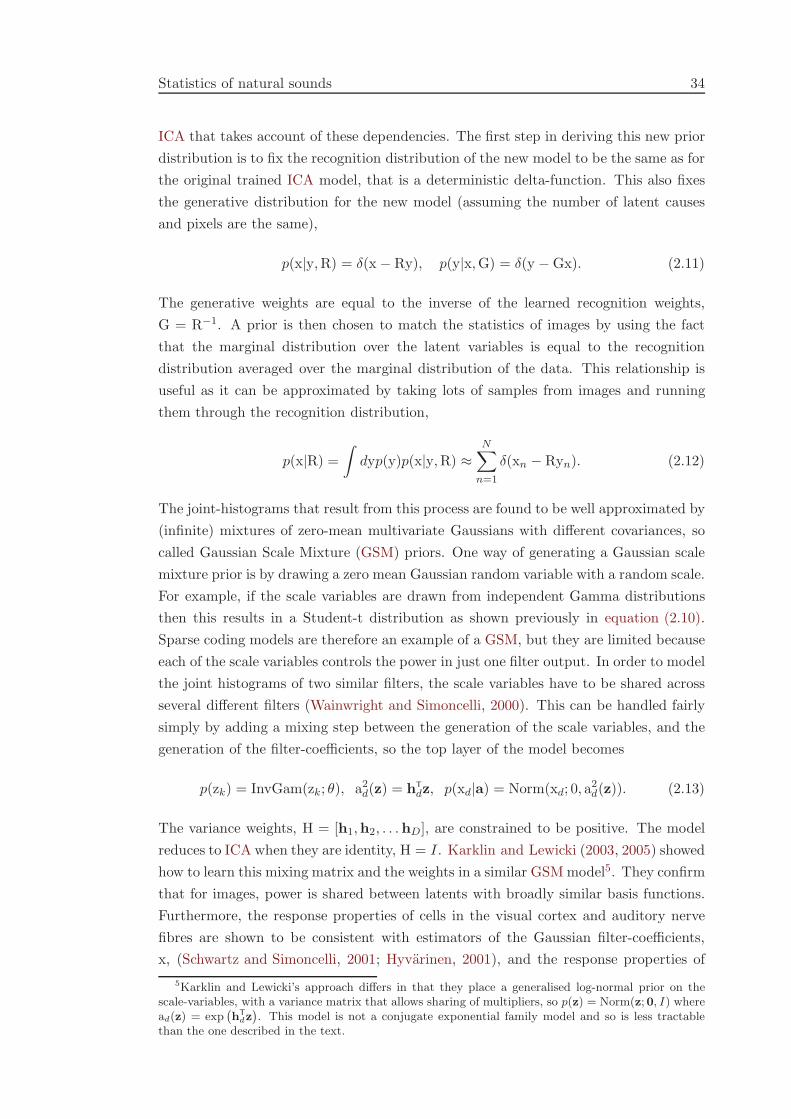
Statistics of natural sounds 34
ICA that takes account of these dependencies. The first step in deriving this new prior
distribution is to fix the recognition distribution of the new model to be the same as for
the original trained ICA model, that is a deterministic delta-function. This also fixes
the generative distribution for the new model (assuming the number of latent causes
and pixels are the same),
p(x|y,R) = δ(x − Ry), p(y|x,G) = δ(y − Gx). (2.11)
The generative weights are equal to the inverse of the learned recognition weights,
G = R−1. A prior is then chosen to match the statistics of images by using the fact
that the marginal distribution over the latent variables is equal to the recognition
distribution averaged over the marginal distribution of the data. This relationship is
useful as it can be approximated by taking lots of samples from images and running
them through the recognition distribution,
p(x|R) =
∫
dyp(y)p(x|y,R) ≈N∑
n=1
δ(xn − Ryn). (2.12)
The joint-histograms that result from this process are found to be well approximated by
(infinite) mixtures of zero-mean multivariate Gaussians with different covariances, so
called Gaussian Scale Mixture (GSM) priors. One way of generating a Gaussian scale
mixture prior is by drawing a zero mean Gaussian random variable with a random scale.
For example, if the scale variables are drawn from independent Gamma distributions
then this results in a Student-t distribution as shown previously in equation (2.10).
Sparse coding models are therefore an example of a GSM, but they are limited because
each of the scale variables controls the power in just one filter output. In order to model
the joint histograms of two similar filters, the scale variables have to be shared across
several different filters (Wainwright and Simoncelli, 2000). This can be handled fairly
simply by adding a mixing step between the generation of the scale variables, and the
generation of the filter-coefficients, so the top layer of the model becomes
p(zk) = InvGam(zk; θ), a2d(z) = hT
dz, p(xd|a) = Norm(xd; 0, a2d(z)). (2.13)
The variance weights, H = [h1,h2, . . .hD], are constrained to be positive. The model
reduces to ICA when they are identity, H = I. Karklin and Lewicki (2003, 2005) showed
how to learn this mixing matrix and the weights in a similar GSM model5. They confirm
that for images, power is shared between latents with broadly similar basis functions.
Furthermore, the response properties of cells in the visual cortex and auditory nerve
fibres are shown to be consistent with estimators of the Gaussian filter-coefficients,
x, (Schwartz and Simoncelli, 2001; Hyvarinen, 2001), and the response properties of
5Karklin and Lewicki’s approach differs in that they place a generalised log-normal prior on thescale-variables, with a variance matrix that allows sharing of multipliers, so p(z) = Norm(z;0, I) wheread(z) = exp
`
hT
dz´
. This model is not a conjugate exponential family model and so is less tractablethan the one described in the text.

Statistics of natural sounds 35
complex cells in the visual cortex are consistent with estimates for the scale variables,
a, (Berkes et al., in press).
The marginal distribution of the data, given the scale variables, is a zero mean Gaussian
distribution, p(y|a, θ) = Norm (y;0,Σy), with a covariance given by,
Σy =
K∑
k=1
zk
D∑
d=1
hk,dgdgT
d. (2.14)
This form connects to Karklin and Lewicki (2008) who model visual data using a zero-
mean Gaussian in which the covariance is given by the matrix-exponential of the above
expression. Further work is required to determine whether the extra flexibility of the
matrix exponential non-linearity is advantageous for modelling natural data.
2.2.2.3 Gaussian Scale Mixtures and Amplitude Modulation
We have now seen several different formulations of GSM models, depending on which
of the latent variables we chose to integrate out. These formulations are summarised
in figure 2.2. In this section we consider a final version of the model that connects
GSM models to amplitude modulation. The treatment of GSMs to this point has been
hierarchical, with the scale variables being generated first, and then the filter coefficients
being drawn conditioned on the scales, and finally the data are drawn. An alternative
view is to draw the scales and normalised filter coefficients at the same time, and then
draw the data using the point-wise product (the un-normalised coefficients),
p(zk) = InvGam(zk; θ), ak(z) = hT
kz, p(ck) = Norm(ck; 0, 1), xk = akck. (2.15)
Now, if GSMs were generalised to a temporal setting and the positive scale variables
imbued with a slower time constant than the normalised coefficients, then the scale vari-
ables would have a natural interpretation as modulators, and the normalised coefficients
as carriers. The implication is that the residual dependencies which GSM models were
developed to handle is due to the presence of strong amplitude modulation in natural
scenes, which is correlated across widely separated filters.
Sparse coding Gaussian Scale Mixture model?>=<89:;z
?>=<89:;x
?>=<89:;x
?>=<89:;a
?>=<89:;y ?>=<89:;y ?>=<89:;y
?>=<89:;z
?>=<89:;x
?>=<89:;a
?>=<89:;a
??
????
???
?>=<89:;c
?>=<89:;y ?>=<89:;y ?>=<89:;y
Figure 2.2: Graphical models for sparse-coding and the GSM.

Statistics of natural sounds 36
2.2.2.4 Modelling Temporal Dependencies
One of the problems with the models for sounds that have been ported over from vision
(PCA, ICA, and GSMs) is that they do not contain an explicit temporal dimension.
To give a specific instance where this is problematic, consider using ICA to model two
sounds which are time-shifted versions of one another. As the basis functions are fixed
to particular positions, the two sounds will activate different sets of basis functions,
and their representation will be quite different. Alternatively, a model with shiftable
basis functions will provide an invariant representation, as well as having other bene-
fits, like the fact that it will be more compact (requiring fewer components), and better
connected to biology. This is the motivation for Smith and Lewicki’s Convolutional In-
dependent Component Analysis (CICA) model (Smith and Lewicki, 2005, 2006) which
assumes that sounds are composed of a set of shiftable basis vectors that have sparse
coefficients6,
xd,i ∼ sparse, yt =
D∑
d=1
I∑
i=1
xd,iWd,t−ti . (2.16)
The shiftable weights can be learned from data using a set of sensible, but heuristic pro-
cedures (for a more principled version see Williams et al. 2007). The resulting weights
bear striking similarity to gammatone functions (Patterson, 1986; Patterson et al.,
1988) which are a popular approximation to the responses of auditory nerve fibres7.
Moreover, the statistics of the centre-frequencies and bandwidths of the learned pop-
ulation match the statistics of natural auditory nerve fibres. One wrinkle that needs
addressing is the fact that when the basis vectors are constrained to be shiftable gamma-
tone functions, rather than general functions, and the parameters of these gammatone
functions are learned from natural speech, the resulting parameters are a poor match to
those encountered physiologically (Strahl and Mertins, 2008). This might be an indi-
cation that the gammatone approximation misses a key aspect of auditory filters which
is captured by the unconstrained learned filters in Smith and Lewicki’s work.
We have described above a family of models (including ICA, sparse-coding, and CICA),
that use sparseness as a heuristic for extracting meaningful components from natural
sounds. In a parallel avenue of research, slowness has also been shown to be a useful
heuristic for extracting meaningful components (Kayser et al., 2001; Wiskott and Sejnowski,
2002; Kording et al., 2004). One example of this approach is the Slow Feature Analysis
(SFA) algorithm which extracts linear projections of the input signal (xk,t = rT
kyt) that
6Smith and Lewicki’s model is an example of CICA which has traditionally been used for blind sourceseparation. For a review of CICA see Pedersen et al. 2008. Another application of related models isto audio-compression. For instance, Hermus et al. (2005) uses damped sinusoids as the shiftable basisfunctions.
7One speculation is that this result could have been obtained using ICA if the number of basisvectors was sufficiently high, so that each basis function could become more specialised.

Statistics of natural sounds 37
are as slow as possible, whilst being decorrelated and of unit variance,
r∗1:K = arg minr1:K
T∑
t=2
(xk,t − xk,t−1)2 such that
1
T
T∑
t=1
xk,txk′,t = δk,k′. (2.17)
This objective is equivalent to maximum-likelihood learning of the weights in a Linear
Gaussian State Space Model, with zero emission noise and independent First order
Auto-Regressive Process (AR(1)) priors over the latent variables (Turner and Sahani,
2007a),
p(xk,t|xk,t−1, λk) = Norm(xk,t;λkxk,t−1, 1 − λ2k), p(yt|xt,G) = δ (yt − Gxt) . (2.18)
The precise equivalence is recovered in the limit as λ1 < λ2 < ... < λK → 0 because then
the maximum-likelihood solution for the generative weights, G∗ = arg maxG log p(y1:T |G),
is equal to the solution from SFA, G∗ = [r∗1, r∗2, ..., r
∗K ]−1.
SFA extracts linear projections of the input signal, but it can be made more powerful
by expanding the input signal though a series of instantaneous non-linearities. It is
well suited to this application, because most non-linear expansions of a signal will be
quickly varying. When the input to SFA is linear and quadratic versions of the pixels
from a movie, the resulting features have many properties in common with complex
cells in the visual cortex (Berkes and Wiskott, 2005), just like the scale variables in a
GSM.
The fact that the variables extracted from natural images using slowness as a heuristic
in SFA resemble the scale estimates from GSM models, suggests that these models are
looking at two sides of the same coin. That is, the real variables are both slow and
modulatory. This is the motivation behind the proof-of-concept “Bubbles” generative
model (Hyvarinen et al., 2003) which has a temporally smooth, sparse prior of the GSM
flavour. The bottom set of weights can be learned using the likelihood as a guide for the
sort of terms that should be present in a suitable cost function. Unlike other models,
however, the neighbourhood of dependence on the multiplier-latents and the temporal
dynamics of the bubble is hard-wired. One of the goals of this work is to generalise
this approach (see Berkes et al. in press for another approach for visual stimuli).
2.2.3 Summary
In summary, there has been significant progress in the statistical modelling of natu-
ral scenes over the past ten years. The evidence from model-based and model-free
approaches is that a suitable generative model for natural sounds should capture
1. the sparse marginal distribution of the waveform,
2. the even sparser marginal distribution of filter activities,

Biological evidence for modulation processing 38
3. the shift invariance of natural sounds (through temporally varying latent vari-
ables)
4. the 1/f spectrum,
5. the complex modulatory structure which is correlated across frequencies and over
many time-scales.
In addition, the inference and learning procedures that are typically used to estimate
generative models of natural scenes, are often quite simple. For instance, Maximum
a posteriori (MAP) inference and Maximum Likelihood (ML) learning are the main
work horses, and it is known that these methods are prone to problems like over-
fitting (MacKay, 2003; Turner and Sahani, in press). Heuristics can be used to avoid
some of the most obvious manifestations of over-fitting. It is common, for example,
to constrain the magnitudes of the filter weights to avoid them blowing up to infinity
whilst the filter-coefficients shrink to zero. However, recent work indicates that there
are more subtle instances of over-fitting which are far less easy to correct heuristically,
like the fact that the estimated filter-weights tend to be more orthogonal than the true
maximum-likelihood weights (Turner and Sahani, in press). One of the focusses of this
thesis is on developing more sophisticated methods that retain as much distributional
information as possible, and which are therefore more robust.
2.3 Biological evidence for modulation processing
One of the main arguments of this thesis is that AM is an important statistical regularity
in natural sounds. If this argument is true then we would expect the organisation and
operation of the auditory system to reflect it. In this section we briefly review evidence
from psychophysics and electrophysiology that suggests that amplitude modulation is
of fundamental importance to auditory processing.
Psychoacoustically, AM impacts many tasks, over a wide range of time-scales (for com-
prehensive reviews see Kay 1982 and Plomp 1983). Amplitude modulation has been
implicated as an important statistic for grouping energy in a signal which comes from
one source, and separating it from energy that comes from another. For example, con-
sider a signal which contains two amplitude modulated tones which are widely separated
in frequency. If the modulation of the tones is independent, then each component can
be heard out from the mixture. However, if the tones are comodulated, then they fuse
and it is very difficult to hear out the individual components (Yost et al., 1989; Moore,
2003). This suggests that common patterns of amplitude modulation across frequency
channels are used to group energy in the signal (Bregman, 1994). Further evidence for
this fact comes from Remez et al. (1981) who show that sinusoidal speech sentences
consisting of three tones are much more intelligible when the tones are comodulated.
Grouping by common AM is important in the well-known phenomenon of Comodulation

Biological evidence for modulation processing 39
Masking Release (CMR). Here, a tone masked by noise with a bandwidth greater than
an auditory filter, becomes audible if the noise masker is amplitude modulated (see
Haggard et al. 1990; Verhey et al. 2003; Moore 2003 for reviews). It appears that the
comodulation of the noise energy in adjacent auditory filters allows the noise component
to be subtracted out and therefore causes the tone to be released from the noise masker.
Interestingly, there is still a release from masking when the modulated noise is presented
contralaterally (Hall et al., 1984). This indicates that AM can be comparable in power
to location as a grouping cue.
Eddins and Wright (1995) investigate CMR when there are multiple time-scales of mod-
ulation. Specifically, the modulation in their experiments had both slow and fast time-
scales and conditions were constructed where one, both, or neither of the time-scales
of modulation were correlated across frequency. They found that the CMR increased
when both time-scales of modulation were correlated. The conclusions from these ex-
periments is that the auditory system processes envelope information across frequency
channels and over multiple time-scales.
Electrophysiological data on the encoding of AM also point to an important role in au-
ditory processing. Although the data are still patchy, it is known that envelope informa-
tion is abundant at the first stage of the auditory system: Type-I auditory nerve fibres
phase-lock to the envelope of sounds (as well as their fine structure) and each nerve fibre
transmits information over a stereotypical range of modulation frequencies, carrier fre-
quencies and intensities (Joris et al., 2004). Moving along the neuraxis to the cochlear
nucleus and then to the inferior colliculus, the tuning to AM typically shows larger gain,
smaller bandwidth (200-300Hz) and the tuning changes from low-pass to more band-
pass. Interestingly, there is evidence for a tonotopic mapping of modulation frequency
sensitivity in the inferior colliculus, running perpendicularly to the carrier frequency
tonotopy (Langner and Schreiner, 1988), although this finding is still debated. Little is
known about cortical processing of AM, but temporal coding of AM seems to be limited
to modulations lower than 30Hz. Interestingly, and unlike lower levels of auditory pro-
cessing, the bandwidth of this tuning appears to be independent of the centre frequency
of the cell, suggesting that there is now independent processing of modulation frequency
in each spectral band. This, and other evidence, has led some authors to propose that
cortex carries out a type of modulation filter bank analysis (Bacon and Grantham,
1989; Dau et al., 1999; Derleth and Dau, 2000; Ewert and Dau, 2000; Houtgast, 1989;
Moore and Sek, 2000; Moore et al., 1999; Strickland and Viemeister, 1996), but this is
a controversial topic (Sek and Moore, 2002, 2003). Although there is a skeptical per-
spective that the electrophysiological results are epiphenomena, there is an opposing
view that amplitude modulation is a fundamental organising principle of the auditory
system (Joris et al., 2004).
The conclusion is that there is a wealth of evidence that AM is important behaviourally,
but it is not completely clear that this is reflected in the neural organization.

Conclusion 40
2.4 Conclusion
This concludes the introductory material which has argued that AM is one of the most
important statistical regularities in natural sounds. The evidence for this argument has
come from three sources. First, we have seen that modulation signatures of sounds are
critical for speech-recognition, speaker-recognition, sound retrieval, cochlear implant
processing and computational auditory scene analysis. This appears to indicate that
the modulation content of natural sounds is a defining characteristic which facilitates
classification. Second, statistical work confirms the conclusion that the modulation
in natural sounds is extremely rich, showing dependencies both across multiple time-
scales and over widely separated sub-bands. Thirdly, it appears that the auditory
system reflects these statistical regularities because it is sensitive to changes in the
statistics of amplitude modulation across multiple time-scales and widely separated
auditory channels.
Finally, although modulation is known to be important, traditional methods for esti-
mating it have many undesirable properties. Despite half a century of attention, there is
no consensus on a de facto estimation method. Model-based statistical approaches offer
a potential alternative. In fact, there appears to be unconscious convergence toward
models with implicit modulators in the natural scene statistics literature. However, a
proabilistic model which treats modulation explicitly is yet to be developed.

Chapter 3
Probabilistic Amplitude
Demodulation
Amplitude demodulation is the task of decomposing a signal into the product of a slowly
varying, positive, modulator and a quickly varying (positive and negative) carrier. In
many applications, traditional approaches to amplitude demodulation perform poorly
when they are applied to natural sounds. For example, in figure 3.1 a short section of
speech has been demodulated using the HE and SLP demodulation methods. The figure
illustrates that the HE contains a contribution from the pitch of the sound and therefore
varies rather quickly. This can be undesirable if we are interested in longer time-scales
of modulation like those associated with the phonemes (Sell and Slaney, submitted).
Unfortunately the HE does not have a parameter which determines the time-scale
of the extracted modulation and so there is no way of controlling this. In contrast,
the SLP method can return an accurate estimate of the envelope (in a squared error
sense), by judiciously setting the low-pass filter cut-off. However, the associated carrier
estimate is often extremely poor, containing large discontinuities. In fact, if the carrier
is demodulated using the SLP method, a rich envelope is recovered indicating that the
signal has not been effectively demodulated. In addition to these practical concerns,
traditional methods for demodulation also suffer from several important theoretical
problems that have been reviewed in section 2.1.1.
Motivated by these deficiencies, we propose a new approach to demodulation which is
to treat it as an inference problem. The new approach is called Probabilistic Amplitude
Demodulation (PAD) because the language of inference is probability theory (Jaynes
2003 and see chapter 1). PAD will be shown to outperform traditional methods (see
figure 3.1 for an example). We will argue that the method is successful because the in-
ferential approach to demodulation is the most natural. This is because demodulation
is fundamentally ill-posed; any positive modulator defines a valid carrier, via division of
the signal. As such, prior information, like the slowness of the envelopes, must be lever-
aged in order to select one of the infinity of valid decompositions. One of the deficiencies

42
0aHE
t
0
aSLP
taP
AD
t
−1
0
1
cHE
t
−50
0
50
cSLP
t
4.65 4.7 4.75 4.8 4.85 4.9 4.95 5 5.05 5.1 5.15
−2
0
2
time /s
cPA
Dt
Figure 3.1: A short segment of spoken speech demodulated using the HE method(top two panels), the SLP method (middle two panels) and PAD (bottom panel).The speech signal is shown in black and the envelopes are shown in red. Theassociated carriers are shown in blue. The solution from PAD is shown along withestimates of the uncertainty (red shaded area).
of traditional approaches to demodulation is that these prior assumptions are implicit,
and this makes it difficult to understand and improve the methods. In contrast, the
inferential approach serves to make the unavoidable assumptions that determine the
solution, explicit. This thesis is testament to the advantages of this approach because
it develops a sequence of models, each of which generalises the assumptions of the pre-
vious. We start in this chapter with simple models for demodulation. In subsequent
chapters, these models are generalised to those containing hierarchies of modulators
with different time-scales (see chapter 4), and finally to sub-band demodulation (see
chapter 5). This progression benefits greatly from the fact that there is an extensive
range of methods for probabilistic inference which can be tapped into. These methods
are slower than traditional methods, because the decomposition has to be iteratively re-
fined via optimisation of a non-linear cost function. However, because the cost-function
embodies the modelling assumptions, this also makes them more accurate.
Ill posed problems, like demodulation, cannot be solved with certainty because there is
not sufficient information to do so. This means that the full solution to a demodulation
problem includes an estimate of the uncertainty. This uncertainty information is poten-
tially useful, for instance if the modulation is being used to compute a decision e.g. in
speaker-recognition. One of the contributions of this chapter is to provide methods for

Simple Probabilistic Amplitude Demodulation 43
estimating the uncertainty in the envelope and carrier variables (see figure 3.1). The
ability to handle uncertainties enables the range of demodulation tasks to be gener-
alised to those involving simultaneous demodulation and denoising, or to fill-in missing
data (see section 3.4).
One of the features of the SLP method is that it has a free parameter which has to
be tuned for each signal. On one hand this is an advantage, because natural signals
often contain multiple time-scales of modulation, and this flexibility enables the user
to select the time-scale of interest. One the other hand, this can be a disadvantage
because it means the method is not fully automated. In contrast the HE does not have
a free-parameter, meaning it is fully automated, the drawback being that the recovered
envelope often has a different time-scale from that which is desired. This chapter will
provide methods for PAD of both sorts. Importantly, the methods with free-parameters
can be turned into automatic methods by learning the free-parameters, for example by
maximum-likelihood.
One of our main motivations for improving traditional methods for estimating ampli-
tude demodulation is to provide more accurate methods for analysing the statistics of
sounds. This chapter concludes with a summary of the sub-band modulation structure
of natural sounds. The conclusion is that the modulation content of natural sounds,
as measured by the statistical modulation depth, is large, and that it spans many
time-scales, from milli-seconds in bird song, to hundreds of milli-seconds in speech.
Moreover, modulation in widely separated channels is often dependent. These types of
statistics can be used to categorise sounds.
3.1 Simple Probabilistic Amplitude Demodulation
This chapter begins by introducing a simple probabilistic model for amplitude mod-
ulation and then goes on to derive an inference procedure called Simple Probabilistic
Amplitude Demodulation (S-PAD). The purpose of studying this model is to clearly
illustrate the probabilistic approach to demodulation and the fact that it performs well
in spite of its simplicity. This is used to motivate several extensions to the basic model.
3.1.1 The forward model
The defining feature of forward models for amplitude modulation is that they comprise
a positive, slowly varying envelope (at) which multiplies a quickly varying real-valued,
(positive and negative) carrier (ct) to produce the data (yt). In the following, the car-
rier will be assumed to be white noise. This is often a severe approximation (e.g. for
natural scenes where the carrier contains pitch and formant information), but in prac-
tice it is found to work surprisingly well because a separation in the time-scales of
the carrier and envelope is sufficient to enable accurate inference. Finally, the positive

Simple Probabilistic Amplitude Demodulation 44
envelope process is produced by taking a slowly varying real-valued process – hence-
forth called the transformed envelope (xt) – and passing it though a static positive
non-linearity. For simplicity, this static non-linearity will be the exponential function,
at = exp(xt). Possibly the simplest way to generate a real-valued slowly varying process
is to use a Gaussian random walk produced by an AR(1) process1 (Chatfield 2003 and
see appendix C). This completes the specification of the forward model which can be
written thus,
p(ct) = Norm(ct; 0, σ2c ), (3.1)
p(xt|xt−1) = Norm(xt;λxt−1, σ2x(1 − λ2)), p(x0) = Norm(0, σ2
x) (3.2)
yt = ctat = ct exp(xt). (3.3)
The AR(1) process is parameterised so that it has marginal variance σ2x and a typical
time-scale which is determined by λ according to τeff = −1/ log λ. For slow envelopes
λ ≈ 1 and so the effective time-scale becomes, τeff = −1/ log(1 − δ) ≈ 1δ . A typical
sample from this generative model is shown in figure 3.2.
0
10
20
30
a t
−0.2
0
0.2
c t
0 200 400 600 800 1000 1200 1400 1600 1800 2000
−5
0
5
y t
time /samples
Figure 3.2: A sample from S-PAD with parameters, λ = 0.99, σ2x = 2, and
σ2c = 0.01. The top panel shows the slowly varying, positive, envelope (red). The
time-scale is about τeff ≈ 100, as illustrated by the black bar. The middle panelshows the quickly varying, positive and negative carrier (blue). The bottom panelshows the generated data (black), which is a product of the envelope and thecarrier variables.
1This connects to Athineos and Ellis (2007) who use Auto-Regressive (AR) processes to modelenvelopes derived using the HE method directly.

Simple Probabilistic Amplitude Demodulation 45
3.1.2 Relationship with existing models
In the generative model above the carriers are treated explicitly, but as the carriers
and modulators are deterministically related to the data, p(yt|at, ct) = δ(yt − ctat), it
is simple to integrate out the carriers, in which case
p(yt|xt, σ2c ) =
∫
dctp(yt|xt, ct)p(ct|σ2c ) = Norm(yt; 0, σ
2ca(xt)
2). (3.4)
That is, each observation is drawn from a zero mean Gaussian with a variance given by
the product of the carrier variance and the square of the envelope variable at that time-
step. This identifies the model as a one dimensional, temporal, Gaussian Scale Mixture
(see section 2.2.2.2). In most of the following the carriers will be treated implicitly
in this manner, and can be recovered by dividing the observations by the envelope,
ct = yt/at.
This simple version of PAD is actually an example of a discrete-time stochastic volatil-
ity model, which are popular in the finance literature (Harvey et al., 1994). In this
setting the data, yt, are returns (e.g. from a stock exchange) and the log-amplitudes,
xt, are the volatility of the returns. The goal is to predict future returns, and the uncer-
tainty in these future returns for use e.g. in options pricing. Stochastic volatility mod-
els are themselves related to Generalised Autoregressive Conditionally Heteroscedastic
(GARCH) models (Engle, 1982). In a GARCH(τ1,τ2) model the amplitude variables are
deterministically related to the previous values of the observations and the amplitudes,
a2t = α0 +
τ1∑
t′=1
αt′y2t−t′ +
τ2∑
t′=1
βt′a2t−t′ . (3.5)
The stochastic volatility models are often preferred to GARCH models because the use
of a stochastic amplitude variable makes them more flexible and a better fit to financial
data. Recent work has focused on generalising the basic stochastic volatility model
e.g. to multivariate time-series, as well as on developing better parameter estimation
methods e.g. via approximate maximum-likelihood (see Shephard and Andersen 2009
for a review). Although the focus in this thesis is on modelling natural sounds, it is
possible that some of the techniques used to generalise PAD are of direct relevance to
practitioners of stochastic volatility models.
PAD is also related to Gaussian Process (GP) models for non-stationary observation
noise. For example, Goldberg et al. (1998) and Kersting et al. (2007) both model ob-
served data as being drawn from a GP and then corrupted by Gaussian noise whose
variance is given by a second, exponentiated, GP. Typically, these models are used
in a regression setting where the task is to estimate the predictive mean (or mode)
from unevenly sampled, noisy data. In this chapter, the goal is rather different, being
estimation of the time-varying variance of the signal in regularly sampled data.

Simple Probabilistic Amplitude Demodulation 46
The probabilistic approach to demodulation was introduced by Turner and Sahani
(2007b). This chapter extends this work by improving the sophistication of model
and introducing methods for handling noise, missing data, and computing error-bars.
An alternative line of research focuses on improving the inference step. Currently, all
versions of PAD employ an inference scheme based on optimisation of a non-linear cost
function. This is potentially problematic as the cost function can have multiple min-
ima, although this has not been observed experimentally. Recently, in an elegant paper,
Sell and Slaney (submitted) develop a convex alternative, which uses the machinery of
convex optimisation (Boyd and Vandenberghe, 2004) in a fast inference scheme. Like
PAD, this method is more robust than traditional demodulation techniques, e.g. to
additive noise. The connections between the present work and Sell and Slaney’s are
discussed in more detail in appendix D. In particular, we show that their approach is
equivalent to a generative model in which the envelopes are generated from a truncated
Gaussian, and the carriers from a uniform distribution between ±1.
3.1.3 Inference
A key quantity in any PAD model is the joint probability of the observations and the
transformed envelopes,
p(y1:T , x0:T |θ) = p(x0)
T∏
t=1
p(yt|xt, θ)p(xt|xt−1, θ). (3.6)
The joint distribution has a complicated dependence on the transformed envelopes due
to the two non-linearities present in the model; the product of the envelopes with the
carriers and the exponential transform between transformed envelope and the envelope.
For this reason it is analytically intractable to calculate the posterior distribution over
the transformed envelope, p(x0:T |y1:T , θ). Therefore, approximation methods are nec-
essary and the most simple, but coarse, option is to calculate the MAP value of the
posterior. That is,
xMAP0:T = arg max
x0:T
p(x0:T |y1:T , θ) = arg maxx0:T
p(y1:T , x0:T |θ). (3.7)
This cost-function can be optimised using a gradient based method such as the con-
jugate gradient method (Atkinson, 1988). For completeness the explicit form of the
objective and its gradients is given in section F.1.1 in the appendices2.
2An alternative procedure, which was used in earlier versions of this work (Turner and Sahani,2007b), is to find the MAP envelope (rather than the MAP transformed envelope). This yields verysimilar results, but it is considerably slower due to the Jacobians introduced from transforming theprior over transformed envelopes into a prior over envelopes, p(a) = p(x)| dx
da|. For this reason the
method described in the text is to be preferred.

Simple Probabilistic Amplitude Demodulation 47
3.1.4 Results and Improvements to S-PAD
S-PAD performs surprisingly well when applied to speech (see figure 3.3). It can recover
phoneme time-scale modulators, which the HE method cannot, and the carriers are
well-behaved, unlike those derived using the SLP method. The success of this simple
−5
0
5
ampl
itude
0 0.5 1 1.5
−3
−2
−1
0
1
2
3
time /s
carr
ier
Figure 3.3: S-PAD applied to a speech sound. The top panel shows a spokensentence (black) which was demodulated using S-PAD. The inferred envelope(shown in red) and the inferred carrier (shown in the bottom panel in blue) areboth of a high quality when compared to existing demodulation approaches.
algorithm indicates the power of the probabilistic approach to demodulation. However,
it is clear that both the model, and the inference/learning can be improved in a number
of important ways.
Improvements to the model:
• The model for the dynamics of the transformed envelopes, an AR(1) process,
is simplistic. For instance, dynamics of natural envelopes are often smooth
(e.g. the phonemes of speech), but a sample from an AR(1) process is not (com-
pare figure 3.2 and figure 3.3). More generally, the spectra of natural modulators
are often complex, and therefore a poor match to the spectrum of an AR(1) pro-
cess which is an exponential with a decay controlled by λ. In section 3.2.5.2, the
model is extended in order to provide methods for learning the time-scale of a
smooth-modulator, and, in section 3.3.2, for learning the entire spectrum of the
transformed envelope process.
• It is clear that natural sounds have a rich carrier structure. For instance, in the
speech example above the carrier includes formant and pitch information. Clearly

Simple Probabilistic Amplitude Demodulation 48
white noise is therefore a terrible model for the carriers in natural sounds. In
section 3.3.2, the model is extended so that the carrier spectrum can be inferred.
• There are three important properties of natural envelopes. The first two are the
mean and the variance, as these control the modulation depth and the overall
variance of the data. The third property is the skewness or asymmetry of the en-
velope. This is important as many natural sounds, like speech, contain envelopes
whose means are small, but which contain regions where the envelope is large.
This results in a skewed distribution. Turning to S-PAD, the variance of the data
and the modulation depth are controlled by σ2c and µ. However, there is no way
to independently control the skew. For this reason a different non-linearity is pro-
posed in section 3.2.1 which is more flexible and a better match to the marginal
distribution of envelopes encountered in natural scenes.
Improvements to inference and learning:
• One of the consequences of viewing demodulation as an ill-posed problem, and
therefore a task of probabilistic inference, is that there are uncertainties in the
envelope estimates. For example, in S-PAD, if the envelope is very slowly varying,
neighbouring data-points will have very similar variances and so the inference
process will effectively average over a large number of samples to estimate the
envelope. The associated uncertainties will therefore be small. For quickly varying
envelopes, the converse is true, and the uncertainty will be large. Computing an
estimate of these uncertainties will be useful, for instance if a decision has to be
computed or if there is a region of missing data in which an envelope must be
estimated. Methods are developed for this purpose in section 3.2.4.
• When faced with a natural sound, it is unclear a priori how to set the parameters
in S-PAD. An incorrect setting can result in a very different envelope estimate.
For this reason it is necessary to to develop methods for learning the parameters
in the model (see section 3.2.5).
• Traditional approaches to demodulation have focussed entirely on the task of
estimating a modulator from complete data. The probabilistic perspective imme-
diately generalises the range of demodulation tasks to those involving noise and
missing data. We provide methods for these tasks in section 3.5.3.
• Natural scenes contain information both at very high frequencies (e.g. the stops
in speech), and very low frequencies (e.g. sentences). This means that they have
to be recorded at very high sampling rates, and over long time scales. Therefore,
the methods developed above must be practical for large data-sets with T ∼ 105−106 samples. In section 3.2.2 it is shown how to construct models for envelope
demodulation that enable the use of the Fast Fourier Transform to accelerate
learning and inference algorithms.

Gaussian Process Probabilistic Amplitude Demodulation 49
3.2 Gaussian Process Probabilistic Amplitude Demodulation
Gaussian Process Probabilistic Amplitude Demodulation (GP-PAD) builds on the
framework of S-PAD. Like S-PAD, it comprises a prior over carriers and transformed
envelopes, which are then combined via a point-wise product to deterministically pro-
duce the data. However, the distributions over both the carriers and the transformed
envelopes are considerably more complicated, both being stationary GPs (details in
the next section) (Rasmussen and Williams, 2006). One of the potential drawbacks of
using GPs is that inference can become computationally costly. However, after describ-
ing the forward model in the next section, we describe a method which augments the
model with ‘missing data’ so that the potentially costly computations can be computed
using the Fast Fourier Transform (FFT) algorithm (section 3.2.2). This leads to effi-
cient algorithms for MAP inference (section 3.2.3). Furthermore, these methods can
be used in combination with the Lanczos algorithm to produce approximate Laplace
error-bars on the MAP estimates (section 3.2.4). Finally, methods are described for
learning all of the free parameters in the model by approximate maximum-likelihood
(section 3.2.5).
3.2.1 Forward Model
The forward model for GP-PAD can be written as follows,
p(x1:T |µ1:T ,Γ1:T,1:T ) = Norm(x1:T ;µ1:T ,Γ1:T,1:T ), µt = µ, Γt,t′ = γ|t−t′|, (3.8)
at = a(xt) = log(1 + exp(xt)), (3.9)
p(c1:T |Φ1:T,1:T ) = Norm(c1:T ; 0,Φ1:T,1:T ), Φt,t′ = φ|t−t′|, (3.10)
yt = atct. (3.11)
That is, both the carriers and the transformed envelopes are produced from stationary
Gaussian processes, with covariance functions γ|t−t′| and φ|t−t′| respectively. Typically,
the frequency content of the transformed envelope process will be concentrated on
frequencies lower than that of the carrier process. With this in mind, a standard choice
for the transformed envelope covariance function is the squared-exponential kernel,
γ|t−t′| = σ2x exp
(
− 1
2τ2eff
(t− t′)2)
. (3.12)
A typical sample from this covariance kernel has a time-scale of ≈ τeff. More generally,
there can be overlap between the spectra of the two processes, as is the case for S-PAD
where the carrier is white noise. Standard demodulation methods often struggle in this
regime.

Gaussian Process Probabilistic Amplitude Demodulation 50
The two remaining differences between S-PAD and GP-PAD are the use of a richer non-
linear mapping from the transformed envelopes to the envelopes, and the fact that the
transformed envelopes have a non-zero mean, µ. The non-linearity, illustrated schemat-
ically in figure 3.4, is called the soft threshold-linear function because it is exponential,
and therefore small, for large negative values of x, and linear for large positive values.
This transforms the Gaussian marginal of the transformed envelopes into a sparse dis-
tribution over envelopes, which is often a good match to the marginal distributions
of natural envelopes (see section 2.2.1). The mean of the transformed envelopes, µ,
controls how close a typical data point is to this transition from exponential to linear.
Together with the marginal variance of the transformed envelopes (σ2x), it alters the
degree of sparsity. A typical sample from this generative model, which is amplitude
−5 −4 −3 −2 −1 0 1 2 3 4 5
x
p(x)
0
1
2
3
4
5
6
p(a)
a
Figure 3.4: A schematic illustrating the mapping from transformed envelope tothe envelope called the soft-threshold function (parameters are σ2
x = σ2c = µ =
1). The marginal distribution over the transformed envelope variable is Gaussian(bottom panel). This is mapped into a sparse marginal distribution over positiveenvelopes (shown in the left panel). The non-linear mapping (large panel, blackline) is exponential for small transformed envelopes (red dashed line) and linearfor large transformed envelopes (blue dashed line).
modulated coloured Gaussian noise, is shown in figure 3.5 and this sound can be found
in the archive ( http://tinyurl.com/archivesounds).
3.2.2 Efficient inference using circular data
The forward model for GP-PAD described in the previous section contains GP priors
over the carriers and the transformed envelopes that take the same general form,
p(z1:T |θ) = det(2πΓ1:T,1:T )−1/2 exp
(
−1
2(z1:T − µ)TΓ−1
1:T,1:T (z1:T − µ)
)
. (3.13)

Gaussian Process Probabilistic Amplitude Demodulation 51
0
1
2
3
a t
−4
−2
0
2
4
c t
3 3.5 4 4.5 5 5.5 6
−5
0
5
time /s
y t
FT
(a)
FT
(c)
0 1000 2000 3000 4000
frequency /Hz
FT
(y)
0 20 40
Figure 3.5: A sample from the GP-PAD generative model produced using pa-rameter values learned from a natural speech sound. The left hand column ofpanels show the components of the generative model in the time domain, and theright hand column of panels show them in the frequency domain. The top rowof panels show the slowly varying envelopes which have energy below about 20Hz(see inset). The middle row of panels show the quickly varying carriers which havea complicated spectra due to the complex fine structure of speech. The bottomrow shows the generated signal which is a modulated version of the carrier. Themodel is clearly much richer than S-PAD.
This expression contains two troublesome quantities; the determinant of the covariance
matrix, det(Γ1:T,1:T ), and multiplication of the data by the inverse covariance matrix,
−12(z1:T −µ)TΓ−1
1:T,1:T (z1:T −µ). Both of these terms have a cost of order T 3 to compute
and therefore intractable for datasets with about T > 103 samples. This is a problem
as a few seconds of a recording of a natural sound will be composed of T ∼ 104 − 106
samples. One way round this obstacle is to introduce a new set of unobserved variables,
zT+1:T ′ , where T′
= 2(T − 1). These new variables are chosen so that the complete
set of augmented variables, z1:T′ are circularly correlated. On the face of it, almost
doubling the number of latent variables appears a peculiar way to alleviate the problem,
but because this places the augmented latent variables on a ring, the new covariance
matrix (Γ1:T′,1:T
′ ) becomes circulant (see figure 3.6),
p(z1:T ′ |µ,Γ1:T ′ ,1:T ′ ) = Norm(z1:T ′ ;µ,Γ1:T ′ ,1:T ′ ), µt = µ, Γt,t′ = γmod(t−t′,T ′).
In turn, this means that matrix operations like multiplication, matrix inversion, and
calculation of determinants follow via the Discrete Fourier Transform (DFT) (see

Gaussian Process Probabilistic Amplitude Demodulation 52
appendix A). For example, the problematic quadratic form can be written,
1
2(z1:T ′ − µ)TΓ−1
1:T ′ ,1:T ′ (z1:T ′ − µ) =1
2∆zT
1:T ′Γ−11:T ′ ,1:T ′∆z1:T ′ , (3.14)
=1
2T′
T′
∑
k=1
|∆zk|2γk
. (3.15)
Where the two new quantities are the DFT of the mean shifted transformed-envelopes
∆zt = zt − µ, and the DFT of the covariance function, which is the spectrum of the
GP.
∆zk =
T′
∑
t=1
FTk,t(zt − µ), γk =
T′
∑
t=1
FTk,tγt, (3.16)
FTk,t = exp(−2πi(k − 1)(t− 1)/T′
), FT−1t,k =
1
T ′exp(2πi(k − 1)(t− 1)/T
′
). (3.17)
These expressions will be of great use in the next sections where they are used to form
an efficient inference method for the transformed envelopes in GP-PAD. Practically,
they can be computed using the FFT.
y1
x1
y2
x2 y
3x
3
......
yT−2
xT−2
yT−1
xT−1
yT
xT
xT+1
xT+2
...
x2T−3
x2(T−1)
Figure 3.6: Graphical model for GP-PAD. The latent variables are drawn from ajoint Gaussian and therefore correlated with one another (hence the central factornode). The latent variables are arranged on a ring, which is to say the correlationbetween a pair of variables depends on their separation measured around the ring.An observation yt is conditionally independent given the latent xt, whence thedirected edges.
3.2.3 MAP Inference
There are two non-linearities in GP-PAD and so exact inference is analytically in-
tractable, just as it was for S-PAD (see section 3.1.3). The simplest form of approximate
inference is to integrate out the observed carriers and find the most probable setting of
the other latent variables, given the data. This inference can be made computationally
efficient by leveraging the FFT. In order to simplify the presentation, we first consider
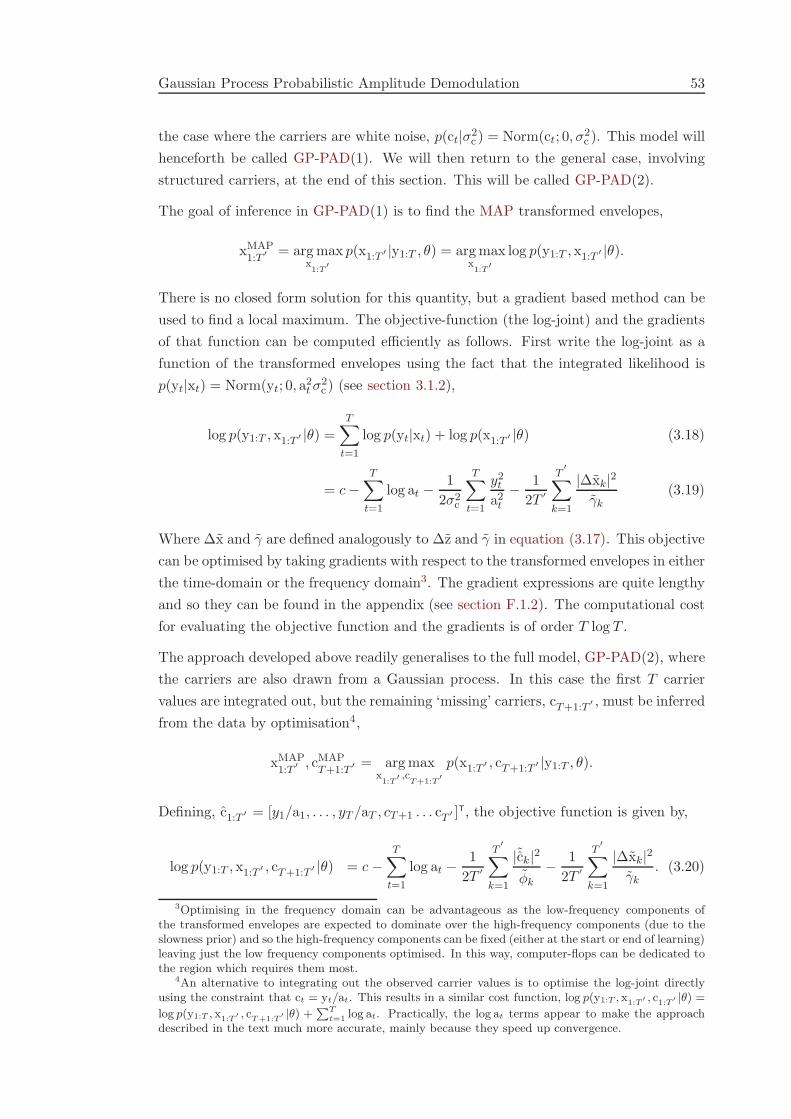
Gaussian Process Probabilistic Amplitude Demodulation 53
the case where the carriers are white noise, p(ct|σ2c ) = Norm(ct; 0, σ
2c ). This model will
henceforth be called GP-PAD(1). We will then return to the general case, involving
structured carriers, at the end of this section. This will be called GP-PAD(2).
The goal of inference in GP-PAD(1) is to find the MAP transformed envelopes,
xMAP1:T ′ = arg max
x1:T
′
p(x1:T ′ |y1:T , θ) = arg maxx1:T
′
log p(y1:T , x1:T ′ |θ).
There is no closed form solution for this quantity, but a gradient based method can be
used to find a local maximum. The objective-function (the log-joint) and the gradients
of that function can be computed efficiently as follows. First write the log-joint as a
function of the transformed envelopes using the fact that the integrated likelihood is
p(yt|xt) = Norm(yt; 0, a2tσ
2c ) (see section 3.1.2),
log p(y1:T , x1:T ′ |θ) =T∑
t=1
log p(yt|xt) + log p(x1:T ′ |θ) (3.18)
= c−T∑
t=1
log at −1
2σ2c
T∑
t=1
y2t
a2t
− 1
2T ′
T′
∑
k=1
|∆xk|2γk
(3.19)
Where ∆x and γ are defined analogously to ∆z and γ in equation (3.17). This objective
can be optimised by taking gradients with respect to the transformed envelopes in either
the time-domain or the frequency domain3. The gradient expressions are quite lengthy
and so they can be found in the appendix (see section F.1.2). The computational cost
for evaluating the objective function and the gradients is of order T log T .
The approach developed above readily generalises to the full model, GP-PAD(2), where
the carriers are also drawn from a Gaussian process. In this case the first T carrier
values are integrated out, but the remaining ‘missing’ carriers, cT+1:T′ , must be inferred
from the data by optimisation4,
xMAP1:T
′ , cMAPT+1:T
′ = arg maxx1:T
′ ,cT+1:T
′
p(x1:T ′ , cT+1:T ′ |y1:T , θ).
Defining, c1:T ′ = [y1/a1, . . . , yT /aT , cT+1 . . . cT ′ ]T, the objective function is given by,
log p(y1:T , x1:T′ , cT+1:T
′ |θ) = c−T∑
t=1
log at −1
2T ′
T′
∑
k=1
|˜ck|2φk
− 1
2T ′
T′
∑
k=1
|∆xk|2γk
. (3.20)
3Optimising in the frequency domain can be advantageous as the low-frequency components ofthe transformed envelopes are expected to dominate over the high-frequency components (due to theslowness prior) and so the high-frequency components can be fixed (either at the start or end of learning)leaving just the low frequency components optimised. In this way, computer-flops can be dedicated tothe region which requires them most.
4An alternative to integrating out the observed carrier values is to optimise the log-joint directlyusing the constraint that ct = yt/at. This results in a similar cost function, log p(y1:T , x1:T
′ , c1:T′ |θ) =
log p(y1:T , x1:T′ , c
T+1:T′ |θ) +
PT
t=1 log at. Practically, the log at terms appear to make the approachdescribed in the text much more accurate, mainly because they speed up convergence.
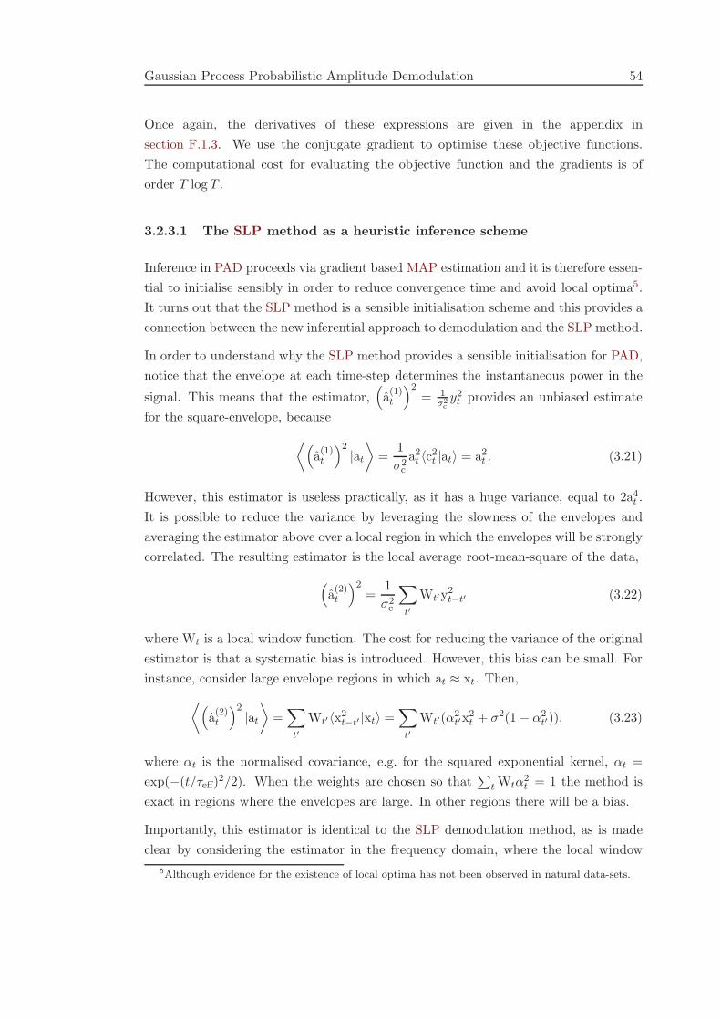
Gaussian Process Probabilistic Amplitude Demodulation 54
Once again, the derivatives of these expressions are given in the appendix in
section F.1.3. We use the conjugate gradient to optimise these objective functions.
The computational cost for evaluating the objective function and the gradients is of
order T log T .
3.2.3.1 The SLP method as a heuristic inference scheme
Inference in PAD proceeds via gradient based MAP estimation and it is therefore essen-
tial to initialise sensibly in order to reduce convergence time and avoid local optima5.
It turns out that the SLP method is a sensible initialisation scheme and this provides a
connection between the new inferential approach to demodulation and the SLP method.
In order to understand why the SLP method provides a sensible initialisation for PAD,
notice that the envelope at each time-step determines the instantaneous power in the
signal. This means that the estimator,(
a(1)t
)2= 1
σ2cy2
t provides an unbiased estimate
for the square-envelope, because
⟨
(
a(1)t
)2|at
⟩
=1
σ2c
a2t 〈c2
t |at〉 = a2t . (3.21)
However, this estimator is useless practically, as it has a huge variance, equal to 2a4t .
It is possible to reduce the variance by leveraging the slowness of the envelopes and
averaging the estimator above over a local region in which the envelopes will be strongly
correlated. The resulting estimator is the local average root-mean-square of the data,
(
a(2)t
)2=
1
σ2c
∑
t′
Wt′y2t−t′ (3.22)
where Wt is a local window function. The cost for reducing the variance of the original
estimator is that a systematic bias is introduced. However, this bias can be small. For
instance, consider large envelope regions in which at ≈ xt. Then,
⟨
(
a(2)t
)2|at
⟩
=∑
t′
Wt′〈x2t−t′ |xt〉 =
∑
t′
Wt′(α2t′x
2t + σ2(1 − α2
t′)). (3.23)
where αt is the normalised covariance, e.g. for the squared exponential kernel, αt =
exp(−(t/τeff)2/2). When the weights are chosen so that∑
t Wtα2t = 1 the method is
exact in regions where the envelopes are large. In other regions there will be a bias.
Importantly, this estimator is identical to the SLP demodulation method, as is made
clear by considering the estimator in the frequency domain, where the local window
5Although evidence for the existence of local optima has not been observed in natural data-sets.

Gaussian Process Probabilistic Amplitude Demodulation 55
becomes a low-pass filter,
(
a(2)t
)2=
1
σ2c
∑
k
FT−1t,k Wky2
k. (3.24)
One important question is how to choose the width of the window. A useful rule of
thumb is to set it equal to about half the expected time-scale of the modulation. This
rule of thumb can be understood by considering a stimulus which contains a low variance
(envelope) region, with high variance regions on either side. If the window function has
a long time-scale then the envelope in the low variance region will be over-estimated.
This is undesirable because inference converges significantly more slowly in regions
where the envelope is over-estimated than in regions where it is under-estimated. This
is a consequence of the fact that a low value of a signal is not unusual in a high-variance
region, whereas a high value of a signal is very unusual in a low-variance region. For
this reason, it is nearly always better to average over a smaller time-scale, than a larger
one.
Finally, we reiterate the fact that although the SLP method often provides a reasonable
estimate of the amplitude, e.g. in a squared-error sense, the corresponding estimate
for the carrier is often extremely inaccurate (see section 2.1.1). Consequently, the
probability of the SLP estimate under the GP-PAD model is often very small and the
gradient-based fine-tuning is essential to recover a good solution.
3.2.3.2 Testing MAP inference
Generally speaking, the MAP estimate of a variable can be a poor one. One common
problem is that MAP solutions can be highly atypical of the posterior distribution
(MacKay, 2003). In order to ensure the quality of the MAP estimate in the current
application, data were generated from the forward model and the MAP approxima-
tion was used to estimate the envelope using the true value of the parameters. This
represents the most favourable situation, because the true parameters are typically
unknown, and therefore serves as an upper limit on the performance which can be
expected when the parameters are unknown. The specifics of the generated data are
as follows: The carrier was chosen to be white-noise and the transformed envelopes
generated using a squared-exponential kernel with time-scales between ten and one
thousand samples. The remaining parameters, the marginal variance and mean of the
transformed envelopes, and the variance of the carriers were sampled from broad uni-
form distributions, σ2c ∼ Uni(1/100, 1/10), σ2
x ∼ Uni(1/100, 1/10) and µ ∼ Uni(−3, 3).
However, as this sometimes resulted in an envelope which has a very small modulation
depth, rejection sampling was used to ensure that the statistical modulation depth6
6The measure of modulation depth used in this thesis is the standard deviation of the modulationdivided by the mean. This definition is proportional to traditional measures and has the advantage ofbeing well defined for stochastic signals. For a discussion, see section 3.5.5.1.

Gaussian Process Probabilistic Amplitude Demodulation 56
was larger than unity, µDet =√
var(at)/mean(at) > 1. Performance was measured by
the Signal to Noise Ratio (SNR) measured in decibels,
SNR = 10 log10
var(
atrue)
var (atrue − aest). (3.25)
The results are shown in figure 3.7, which indicate that the inference process is accurate
over a wide range of time-scales and parameter settings. Accuracy improves as the
time-scale increases because there are more samples of white noise to average over per
time-scale. Roughly speaking, the envelope of a signal of 8000 samples long takes about
5 minutes to calculate on an Inspiron 6400 laptop with 1GB of memory and an Intel
T2400 1.83GHz processor.
10 20 50 100 200 500 10005
10
15
20
25
30
35
true time−scale
sign
al to
noi
se /d
B
50 100 150 200 250 300 350 400 450 5000
0.1
0.2
1000 2000 3000 4000 5000 6000 70000
1
2
0.5 1 1.5 2 2.5 3 3.5 4 4.5
x 104
0
5
10
time steps
Figure 3.7: Testing Maximum a posteriori (MAP) inference. Top panel: SNR ofenvelopes estimated from data generated from the forward model with time-scalesbetween 10 and 1000 time-steps. The other parameters were chosen as describedin the text. The lower panels show several examples of inferred envelopes (red)together with ground truth (black). The time-scales and the SNR values for theseexamples are indicated by the red dots in the top panel. The examples are orderedso that lower panels correspond to higher SNRs and longer time-scales.

Gaussian Process Probabilistic Amplitude Demodulation 57
3.2.4 Error-bars and Laplace’s Approximation
We have now developed an efficient method for demodulation based on a MAP trans-
formed envelope inference. One of the key advantages of framing demodulation as a
task of probabilistic inference is that it provides an opportunity to tap into existing
methods which can provide estimates of the uncertainties in the recovered envelopes.
This is the goal of this section. A major obstacle in the application of standard meth-
ods to PAD is the fact that the number of latent variables is typically very large and
this restricts the choice of approximation scheme considerably. This section describes
how to use an approximate version of Laplace’s method (itself an approximation) to
recover error-bars that accurately reflect uncertainty in the MAP inference described
in the previous section. Although the methods developed here are only theoretically
justified when using GP-PAD in which the carrier is white noise (i.e. GP-PAD(1)),
experiments described at the end of this section indicate that they provide reasonable
estimates when the carrier is structured too. This indicates that the methods can be
used for GP-PAD(2) as well.
Laplace’s approximation (MacKay, 2003) approximates the posterior distribution over
transformed envelopes by a Gaussian with a covariance matrix given by the negative
inverse of the Hessian, H of the log-joint,
p(x1:T′ |y1:T , θ) ≈ det(−H/2π)1/2 exp
(
1
2(x1:T
′ − xMAP1:T ′ )H(x1:T
′ − xMAP1:T ′ )
)
, (3.26)
where,
Ht,t′ =d2
dxtdxt′log p(y1:T , x1:T ′ |θ)
∣
∣
∣
∣
x1:T
′ =xMAP
1:T′
. (3.27)
Upon first consideration it appears fruitless to use Laplace’s approximation to return
error-bars for GP-PAD because the Hessian is a 2(T −1)×2(T −1) matrix and so exact
inversion is intractable for data-sets of even modest size (i.e. T > 1000). However, it
will be shown that the slowness of the transformed envelopes can be leveraged in order
to recover estimates for the marginal variances of the transformed envelopes, that is
the diagonal elements of the approximate posterior covariance matrix.
To see how this is possible, first note that the Hessian is the sum of the Hessian of the
likelihood and the Hessian of the prior. Both of these quantities have simple forms.
The negative Hessian of the likelihood is a diagonal matrix,
Dt,t′ = − d2
dxtdxt′log p(y1:T |x1:T , θ) = dtδt,t′δt≤T . (3.28)
The negative Hessian of the prior is the inverse of the prior covariance matrix, Γt,t′ . This
is positive definite and therefore has a matrix square-root. Moreover, it is diagonal in
frequency space. The expression for the inverse Hessian, equivalently the approximate

Gaussian Process Probabilistic Amplitude Demodulation 58
posterior covariance, can therefore be written as follows,
−H−1 = Σpost = (D + Γ−1)−1 = Γ(DΓ + I)−1 = Γ1/2(Γ1/2DΓ1/2 + I)−1Γ1/2 (3.29)
This new form is helpful because all the important action is in the matrix A = Γ1/2DΓ1/2
(the other terms being simple to compute exactly). The matrix A inherits, from the
prior covariance Γ, the property that only the low-frequency components are strongly
active (see figure 3.8). Consequently A can be well approximated by a truncated eigen-
expansion, A ≈ ∑KMAXk=1 λkeke
T
k. Therefore the problem reduces to finding an efficient
method to compute the top KMAX eigenvectors and eigenvalues of A. Fortunately, the
Lanczos algorithm can do just this for K . 500, requiring just multiplications of A
times a vector (Bultheel and Barel, 1997). These multiplications are fast as they use
the FFT,
0 100 200
10−10
10−5
100
valu
e
eigenvalue number
time−scale = 2
0 100 200
time−scale = 5
0 100 200
time−scale = 10
Figure 3.8: Eigen-spectra of the prior covariance (Γ, blue lines) and the matrixA = Γ1/2DΓ1/2 (red lines) for three different time-scales (l = [2, 5, 10]) whenT = 100. The prior covariance is a squared exponential, plus a small constant(10−12) to avoid numerical problems. The two eigen-spectra are similar, and forlarge time-scales, both are dominated by a small number of eigenvalues. The black
vertical line indicates the truncation criterion, KMAX = Ns(T−1)πτeff
where Ns = 10.
∑
t′
At,t′vt′ =∑
k,t′,k′
FT−1t,k (γk)
1/2FTk,t′dt′FT−1t′,k′(γk′)1/2vk′ (3.30)
The final step is to convert the approximation of A into an approximation for the diag-
onal elements of the posterior covariance matrix. Being careful to make the truncation

Gaussian Process Probabilistic Amplitude Demodulation 59
at the end of the calculation, we find after some work,
(A+ I)−1 ≈ I −KMAX∑
k=1
λk
λk + 1eke
T
k. (3.31)
This can now be substituted into the original expression for the approximate posterior
covariance,
Σpost ≈ Γ1/2
(
I −KMAX∑
k=1
λk
λk + 1eke
T
k
)
Γ1/2, (3.32)
so that the marginal approximate posterior variances can be computed efficiently as
follows,
Σpostt,t ≈ γt −
KMAX∑
k=1
λk
λk + 1
T′
∑
a=1
FT−1t,a γ
1/2a ea,k
2
. (3.33)
This expression has an instructive interpretation; in order to compute the approximate
posterior marginal variances (the posterior uncertainties), begin with the marginal vari-
ances of the prior (the prior uncertainties) and subtract uncertainty from it as more
eigenvalues are considered. One nice property of the eigenvalue truncation is that if
KMAX is set too low, then the error-bars are over estimated (as λk ≥ 0). It is nearly al-
ways better to over-estimate the uncertainty as the use of approximations will increase
our uncertainty in unknown quantities.
3.2.4.1 Experiments and practical considerations
In this section the approximation scheme developed above is tested on a small data-set
(T = 1000) for which Laplace’s approximation can be computed exactly. The data
were generated from the forward model for GP-PAD(1) with a squared exponential
covariance function for the transformed envelopes. The true Laplace error-bars were
calculated and compared to those estimated using the Lanczos approximation (see
figure 3.9). The conclusion is that the Lanczos approximation is extremely accurate as
long as a sufficient number of eigenvalues are retained, and we will provide a definition
of sufficiency in equation (3.35). Furthermore, the experiments were repeated for data
drawn from GP-PAD(2), and the true Laplace error-bars were computed incorporating
the fact that the carriers are coloured noise. When the error-bars are computed using
the Lanczos approach (which treats the carriers as white noise), the error is similar
to that shown in figure 3.9, as long as the carrier and envelope time-scales are well
separated (data not shown).
Practically, the Lanczos algorithm can be used to compute only the top KMAX . 500
eigenvalues as it involves a re-orthogonalisation step after extracting each eigenvalue

Gaussian Process Probabilistic Amplitude Demodulation 60
10 20 30 40 50
40
60
80
100
120
140
160
time−scale
Km
ax
40
50
60
70
80
90
100
110
120
130
140
150
10 20 30 40 50
40
60
80
100
120
140
160
time−scale
−20
0
20
40
60
80
100
120
140
Figure 3.9: Laplace tests. Left hand panel SNR between the true Laplace log-determinant and the approximated log-determinant measured in decibels. Righthand panel: SNR between the true Laplace error-bars and the approximated error-
bars in decibels. In both cases the condition, KMAX = Ns(T−1)πτeff
is shown by thethick black lines where Ns = 10. For the right-hand plot the SNR along thisline is about 106, and for the left-hand plot the SNR is about 105 indicating theapproximation is accurate to at least one part in a hundred thousand in this region.
which has a cost that grows with the cube of the number of the eigenvalues extracted to
that point. This means that long data-sets with quickly varying transformed envelopes
must be split into smaller chunks. The length of these chunks must be chosen so that
number of significant eigenvalues that the matrix A has, is less than about 500. This
can be ensured by considering the eigen-spectrum of the prior covariance, Σ, which is
given by the DFT of the squared exponential covariance function. For long signals, this
is approximately equal to the Fourier Transform and so,
γk ≈ σ2x exp
(
−k2
2
(
2πτeffT
′
)2)
. (3.34)
This is a Gaussian with a standard deviation of T−1πτeff
. As the spectrum of A inherits
this shape, a sensible truncation point is defined by,
KMAX =Ns(T − 1)
πτeff. (3.35)
Here, Ns is the number of standard deviations to retain. This means the maximum
length of a chunk of data is approximately, Tmax = 3NsKτeff. Typical choices are
K = 200, Ns = 10 which means Tmax = 60τeff. This completes the process by which
the error-bars can be computed.

Gaussian Process Probabilistic Amplitude Demodulation 61
3.2.5 Parameter Learning
The previous sections were concerned with inferring the transformed envelope from
data, and with placing error-bars on these inferences, in the case where the parameters
were known. In general it is necessary to learn these parameters as it is not clear
what an appropriate modulator time-scale, or sparsity is for a natural sound. Machine-
learning provides many possible parameter learning schemes, but one of the surprising
conclusions of this work is that many are unsuitable for this application. Some of the
possible strategies are listed in table 3.1, roughly ordered by their complexity, together
with their associated pitfalls. The general conclusion is that the complex methods
are too slow to be used on large data-sets, but the simple methods have pathological
biases that result from a tendency to over-fit the data. The key is to find a method in
the middle ground, that retains uncertainty information in the transformed envelopes
(and therefore avoids the over-fitting pathologies), but which remains computationally
cheap. In fact, experiments indicate that it is useful to split the parameter learning
into two stages. First, the marginal distribution of the data is used to estimate the
carrier variance (σ2c ) and the transformed envelope variance (σ2
x) and mean (µ). The
advantage with considering just the marginal statistics of the data is that the temporal
dependencies between the latent variables can be ignored meaning that they can be
integrated out using one-dimensional numerical integrals. However, it is clear that
the temporal structure of the data is required in order to learn the dynamics of the
modulator. For this reason the second part of the parameter learning process is to
use Laplace’s approximation to the marginal likelihood in order to learn the time-scale
(τeff). As much of the machinery for this has been developed in section 3.2.4 (where
Laplace’s approximation was used to return error-bars), relatively little work is required
to derive this method. However, one of the limitations of using Laplace’s method is that
it is restricted to a GP-PAD model in which the carriers are drawn from a white-noise
process.
3.2.5.1 Learning parameters from the marginal data
The marginal distribution of the data is determined by the marginal statistics of the
carrier, p(c|σ2c ) ∼ Norm(0, σ2
c ), and the marginal statistics of the transformed envelopes,
p(x|µ, σ2x) ∼ Norm(µ, σ2
x). Importantly, it does not depend on the temporal dynamics
of the transformed-envelope or carriers, and therefore it can be computed via a one-
dimensional integral,
p(y|σ2c , µ, σ
2x) =
∫
dx p(y, x|σ2c , µ, σ
2x) =
∫
dx p(y|x, σ2c )p(x|µ, σ2
x). (3.36)

Gau
ssianP
rocess
Prob
abilistic
Am
plitu
de
Dem
odulation
62
Inference Learning Uncertainty Problems
Latent Parameter
maximum a posteriori maximum likelihood No No Over-fitting for all parameters
maximum a posteriori variational Bayes[1] (Maximisation-Expectation algorithm)
No Yes* Over-fitting for all parameters
maximum a posteriori exact integration No Yes Over-fitting for σ2c
variational mean-field [2] Any Yes* ? Slow due to iterated 1D numerical integrals,under-estimates of latent uncertainty cause largebiases in learning
Laplace’s approximation [3] maximum likelihood Yes No Over-fitting for σ2c and σ2
x, good for τeff and µ,
Estimation using marginal statistics(see section 3.2.5.1)
maximum likelihood Yes No Good for σ2c , σ
2x and µ, but no way to learn τeff,
Expectation Propagation [4] Any Yes ? 1D numerical integrals slow
Monte Carlo Markov Chain [5]e.g. Hamiltonian
Any Yes ? Too slow for large data-sets
Table 3.1: Candidate parameter learning methods. Variational methods, marked with a ‘*’, severely under-estimate uncertainty information andthis limits the usefulness of the distributional information that they retain. For more details on the methods in this table, see [1] Beal (1998),[2] Jordan et al. (1999); Wainwright and Jordan (2008), [3] MacKay (2003) , [4] Minka (2001), and [5] Neal (1993).

Gaussian Process Probabilistic Amplitude Demodulation 63
This one dimensional integral is not analytically tractable, but it is relatively simple to
approximate numerically (e.g. by gridding up the space that has significant mass under
the prior). The marginal distribution of the data can be used to learn the marginal
distribution of the carriers and the marginal distribution and mean of the transformed
envelopes, via (approximate) ML. This is a relatively fast approach because it avoids
modelling the temporal correlations in the data, but it is accurate because it incorpo-
rates distributional information about the transformed envelopes.
Practically, ML optimisation proceeds via an initial coarse grid search, followed by local
fine-tuning. The initial coarse grid search is necessary as the likelihood is multi-modal.
During the fine-tuning phase, which performs a local grid-search centred on the current
value of the parameters, momentum updates are used to speed up convergence. These
perform a line-search every N iterations using the combined change in parameters over
the previousN iterations (i.e. ∆θ = θn−θn−N ) to define the direction of the line-search.
In order to test the success of this procedure, data were generated from the forward
model with many different settings of the parameters, and these parameters were
learned using the scheme described above. The results, shown in figure 3.10, indicate
that the estimated parameters are accurate over a wide range.
3.2.5.2 Learning the time-scale using Laplace’s Approximation
The marginal distribution of the data is independent of the time-scale of the modulators
and therefore cannot be used to learn this time-scale. An alternative method is to use
Laplace’s approximation to perform an approximate integration of the transformed
envelopes. This is called Laplace’s approximation for the marginal likelihood,
p(y1:T |θ) =
∫
dx1:T ′p(y1:T , x1:T ′ |θ) ≈ p(y1:T , xMAP1:T ′ |θ) (2π)T−1
√D + Σ−1
,
where, to remind the reader, Σ−1 and D are the negative Hessians of the prior and
likelihood respectively. Using the previously described results (see section 3.2.4), the
log-determinant can be approximated using an eigenvalue truncation,
log det(
D + Σ−1)
≈ −T
′
∑
k=1
log γ +
KMAX∑
k=1
log(1 + λk). (3.37)
The approximate likelihood of the time scales is therefore,
L(τeff) = − 1
2σ2c
T∑
t=1
y2t
a2t
−T∑
t=1
log(at) −1
2T′
T′
∑
k=1
(xk)2
γk
− 1
2
KMAX∑
k=1
log(1 + λk) − (T − 1) log 2πσ2c (3.38)

Gaussian Process Probabilistic Amplitude Demodulation 64
KL: 0µ: 0
KL: 0.03µ: 0.23
KL: 0.05µ: 0.33
KL: 0.08µ: 0.4
KL: 0.11µ: 0.46
KL: 0.13µ: 0.52
KL: 0.16µ: 0.57
0 0.02 0.04 0.06 0.08 0.1 0.12 0.14 0.16
0.51
1.52
2.53
0.5
1
1.5
2
2.5
3
−4
−2
0
2
µ
σc
σa
mean KL
Figure 3.10: Parameter learning tests. Data were generated from the forwardmodel using seven different values for each of the parameters, σ2
c , σ2x and µ. The
range of these parameters was chosen to match that encountered in natural data.The parameters were learned from each data-set using a random initialisation.The quality of the fit was evaluated using the KL divergence between the trueand estimated data probability, KL (p(y|θTrue)||p(y|θEst)). This is indicated bythe colour of each point in parameter space. The top panel shows the mappingfrom the colours to the KL divergence. In order to aid intuition, various valuesof the KL divergence are illustrated schematically using a pair of unit varianceGaussians whose means are appropriately mis-tuned. The conclusion is that overthis range, the parameter learning methods are accurate.
This can be optimised to find the optimal time-scale, τeff, by a grid search. That is,
a range of time-scales are chosen, the MAP transformed envelope solution found for
each, and then the objective function above evaluated to determine the best setting.
Practically a coarse grid search is used initially, whereby a large range of widely sepa-
rated time-scales are tested, followed by a local fine-tuning grid-search centred on the
current value of the time-scale.
In order to test this scheme, data were generated from the forward model with time-
scales from ten to one-thousand samples. The other parameters were generated using
rejection sampling using the procedure described in section 3.2.3.2. The algorithm had
to learn the time-scales, but it was given the true value of the other parameters. The
results shown in figure 3.11 indicate that the method accurately infers the time-scales
over a large range, although there is a small bias to shorter time-scales (typically, the
learned time-scales are 10% smaller than ground truth). Furthermore, the estimated
modulators are a close match to the true modulators. In fact, the difference between

Gaussian Process Probabilistic Amplitude Demodulation 65
envelopes estimated using the true and estimated value of the time-scale is negligible.
10
20
50
100
200
500
1000
estim
ated
tim
e−sc
ale
10 20 50 100 200 500 10000
10
20
30
40
true time−scale
SN
R /d
B
Figure 3.11: Learning the time-scales. The parameters (σ2x, σ2
c , µ) were randomlysampled over the range encountered in natural scenes and the time-scales learnedusing these settings. Top: True time-scale versus inferred time-scale. Groundtruth (red line). Mean and one standard deviation (black line). Individual runs(black points). There is a tendency to under-estimate the time-scale by about10%. Bottom: SNR (measured in decibels) of the inferred modulators as a functionof the time-scale (black) for comparison the results from MAP inferences wherethe time-scales were known (red) (the settings of the other parameters were notidentical). The black and red lines show the average SNR. Although the inferredtime-scales are often under-estimates of the true time-scale, this does not appearto introduce significant error into the inferences for the modulators.
3.2.6 Summary of GP-PAD
This concludes the development of GP-PAD which models data as amplitude modu-
lated white (GP-PAD(1)) or coloured (GP-PAD(2)) noise. We have described methods
for efficient MAP based inference for both of these models, based in the idea of circu-
larising the latent-variables in order to use the FFT. We then showed how to use the
Lanczos algorithm to estimate Laplace error-bars on these inferences. Finally, methods
were provided for learning the marginal parameters of GP-PAD, using the marginal
probability of the data, and also for learning the time-scales of the modulator, using
the same Laplace-Lanczos approximation that is used to estimate error-bars. All of
these procedures were validated on data drawn from the forward model.

Improving the model: SP-PAD 66
3.3 Improving the model: SP-PAD
The previous section developed methods for performing inference and learning in
GP-PAD. There are two key limitations to these methods. The first is that meth-
ods have not been provided for learning the spectral content of the carrier. This is
problematic because natural signals have highly structured carriers, but as it is not
necessarily clear a priori what form this structure should take, it must be learned from
data. The second key limitation of the methods developed in the last section is that the
GP prior over the transformed-envelopes had to be of a fixed parametric form (e.g. the
squared-exponential). This is inappropriate for modulators in natural signals as they
are likely to have more complicated spectra that are not easy to capture through some
pre-specified parametric covariance function. In this section methods are developed for
inferring the spectra of the carriers and of the transformed-envelopes. This requires a
more flexible model than GP-PAD with many extra parameters. Consequently, it is
important to retain a full distribution over all of the components of the spectrum in
order to avoid over-fitting. Importantly, GP-PAD still has an important role to play
as an initialisation scheme for the more complex models.
This section is organised as follows, first we introduce the theoretical framework for
inferring the unknown spectrum of a process (see section 3.3.1). The centre piece
is a prior over signals which models each spectral component as being drawn from
a Student-t distribution. This new Student-t prior replaces the GP prior over the
transformed envelope and carrier processes in GP-PAD, to form a new model called
Student-t Process Probabilistic Amplitude Demodulation (SP-PAD).
3.3.1 Bayesian Spectrum Analysis
This section develops a framework for inferring spectra of discrete GPs. We showed
earlier how to use missing data in order to place variables drawn from a discrete sta-
tionary GP onto a ring (see section 3.2.2). This meant that the GP prior over these
variables could be written in a simple form involving the spectrum of the GP (γk) and
the Fourier coefficients of the latent variables (∆zk),
p(z1:T ′ |γkT′
k=1) =
T′
∏
k=1
(2πγk)−1/2 exp
(
− 1
2T′
γk|∆zk|2
)
. (3.39)
This GP prior is factorised in the frequency domain, because the DFT diagonalises
stationary GP covariance functions (see appendix A). In other words, the GP prior
can be thought of as an independent, zero mean, Gaussian prior over each Fourier
coefficient, with a variance that is specified by the spectrum (see appendix B for an
equivalent ‘weight-space’ view). Armed with this new perspective, it is natural to
extend the existing framework to the case where the spectrum is also unknown and

Improving the model: SP-PAD 67
must be be inferred. This proceeds in two stages; first, priors are be placed on the
unknown spectral components, and second the posterior distribution over the spectral
components derived. One natural choice for the prior on the spectral components is a
product of Independent Inverse Gamma distributions,
p(γk|αk, βk) = InvGam(γk;αk, βk) =βαk
k
Γ(αk)(γk)
−αk−1 exp
(
−βk
γk
)
. (3.40)
Care has to be taken because the spectrum is symmetric, γT−k = γT+k, and so it is
only necessary to place priors over the first T spectral components. The mean and
variance of the inverse-Gamma distribution are
mean (γk) =βk
αk − 1, var (γk) =
β2k
(αk − 1)2(αk − 2). (3.41)
These expressions can be used to set appropriate priors over the spectrum. For example,
a prior over spectra which has a frequency dependent mean and a standard-deviation
in each channel which is a fraction of the mean value of that channel,
mean (γk) = Γk, var (γk) = γ2kΓ2
k (3.42)
can be set by,
αk = γ−2k + 2, and βk = (αk − 1)Γk. (3.43)
The Inverse Gamma prior over the spectral components is a natural choice due to its
conjugacy with the Gaussian distribution over Fourier coefficients. One consequence
is that the prior over spectral components can be integrated out which reveals the
marginal distribution over Fourier coefficients as a product of independent Student-t
distributions (see section 2.2.2.1). In turn, the marginal distribution of the data is a
Student-t process7,
p(∆zk|θ) =
∫
dγkp(∆zk|γk, θ)p(γk|θ) = Student(∆zk; θ), zt = µ+T
′
∑
k=1
FTt,k∆zk
Another consequence of the conjugate priors is that the posterior distribution over
spectral components is simple to derive, being of the same functional form as the prior,
p(γ1:T |z1:T′ , θ) =
T∏
k=1
(
βposk
)αposk
Γ(αposk )
(γk)−αpos
k−1 exp(−βpos
k /γk). (3.44)
7Although not strictly a process, this was named in analogy with the GP by Rasmussen and Williams2006.

Improving the model: SP-PAD 68
where for 1 < k < T
αposk = αk + 1, βpos
k = βk +1
T ′|∆zk|2 , (3.45)
otherwise, for k = 1 or k = T
αposk = αk +
1
2, βpos
k = βk +1
2T′|∆zk|2 . (3.46)
The posterior distribution over the spectral components has a number of interesting
properties. For example, each spectral component is uncorrelated with every other and
so the posterior mean and variance are not smooth functions. In fact, if the contribution
from the prior is small, the mean of the posterior distribution is proportional to the
average energy in the signal at that frequency, and the variance is proportional to the
square of that average-energy. Consequently, the posterior variance of the spectral
components does not decrease as more data are obtained. This may appear counter
intuitive if the spectral components are thought of as parameters. However, because the
number of the spectral components increases with the size of the data-set, they should
be thought of as latent variables. In fact, as the number of time points increases, so
does the frequency resolution of the spectrum, and so it is natural that the uncertainty
in each component stays the same. One of the consequences of the fact that the effective
number of data points per spectral component is small, and remains fixed as we see
more data, is that we are always in the regime where the prior makes a significant
contribution to the inferences made. Finally, we note that the prior introduced in
this section generalises the work of Bretthorst (1988) and connects his formalism to
stationary Gaussian processes. For another perspective on these matters, we again
refer the reader to appendix B.
3.3.2 Bayesian Modulation Spectrum Analysis
The previous section has shown how to hierarchically extend a stationary discrete time
GP prior so that the spectrum can be inferred. In this section, GP-PAD is extended
in this manner, and this requires the addition of independent Inverse Gamma prior
distributions over the spectra of both the carriers and transformed envelopes. The new

Improving the model: SP-PAD 69
model is called SP-PAD and the generative model is,
p(γk|αxk , β
xk ) = InvGam(γk;α
xk , β
xk ), p(∆xk|γk) = Norm(∆xk; 0, γk), (3.47)
xt =T
′
∑
k=1
FT−1t,k∆xk + µ, at = a(xt) = log(1 + exp(xt)), (3.48)
p(φk|αck, β
ck) = InvGam(φk;α
ck, β
ck), p(ck|φk) = Norm(ck; 0, φk), (3.49)
ct =
T′
∑
k=1
FT−1t,k ck, (3.50)
yt = atct. (3.51)
Typically the prior distribution over the spectrum of the transformed envelopes is
chosen so that it contains only low-frequency components. Inference in this new model
proceeds via MAP estimation of the transformed envelopes (xT ′ ) and the ‘missing’
carriers (cT+1:T ′ ) (identically to GP-PAD, see section 3.2.3),
xMAP1:T ′ , cMAP
T+1:T ′ = arg maxx1:T
′ ,cT+1:T
′
p(x1:T ′ , cT+1:T ′ |y1:T , θ) (3.52)
= arg maxx1:T
′ ,cT+1:T
′
log p(y1:T , x1:T ′ , cT+1:T ′ |θ). (3.53)
The objective, which is the log-joint distribution of the transformed envelopes and
missing carriers, is formed from the complete-data joint distribution by integrating the
carriers (c1:T ) and the spectra (γ1:T and φ1:T ),
p(y1:T , x1:T ′ , cT+1:T ′ , θ) =
∫
dc1:T dγ1:Tdφ1:T p(y1:T , x1:T ′ , c1:T ′ , γ1:T , φ1:T |θ). (3.54)
The integration over the spectra results in distributions of the following form over the
transformed envelopes and carriers,
p(z1:T ′ |βk, αkTk=1) =
T∏
k=1
βαk
k(
βposk
)αposk
Γ(αposk )
Γ(αk). (3.55)
Therefore, completing the integration over the two specta and the carriers, results in
the following objective function,
log p(z1:T ′ , cT+1:T ′ , y1:T |θ) =
c+
T∑
k=1
(
αck log βc
k − αc,posk log βc,pos
k + αxk log βx
k − αx,posk log βx,pos
k
)
(3.56)

Improving the model: SP-PAD 70
where for 1 < k < T
αc,posk = αc
k + 1, βc,posk = βc
k +1
T ′
∣
∣
∣
˜ck
∣
∣
∣
2, (3.57)
αx,posk = αx
k + 1, βx,posk = βx
k +1
T ′|∆xk|2 , (3.58)
otherwise, for k = 1 or k = T
αc,posk = αc
k +1
2, βc,pos
k = βck +
1
2T ′
∣
∣
∣
˜ck
∣
∣
∣
2, (3.59)
αx,posk = αx
k +1
2, βx,pos
k = βxk +
1
2T ′|∆xk|2 , (3.60)
and, to remind the reader, c1:T ′ = [y1/a1, . . . , yT /aT , cT+1 . . . cT ′ ]T. The gradients of
this objective function, which can be found in section F.1.4, can be used to find the
MAP estimate using e.g. conjugate gradient optimisation.
One of the problems with joint estimation of the spectra of the carriers and transformed
envelope variables is that it leads to an over-fitting problem whereby the marginal vari-
ance of one of the variables blows up to infinity and the other shrinks to zero. Problems
of this sort plague any PAD learning scheme which fails to incorporate uncertainty in-
formation correctly (see section 3.2.5). In order to ameliorate this effect, it is necessary
to add an extra term to the cost function, which constrains the marginal variance of
the carriers and transformed envelopes, and the mean of the transformed envelopes.
One way of doing this is to add a quadratic penalty between the desired and empirical
statistic, where the target values are determined using the parameter learning schemes
described earlier (see section 3.2.5). The details of this proceedure can be found in the
appendix, see section F.1.4.
3.3.2.1 Error-bars
It is simple to use the Lanczos-Laplace error-bar estimation approach, described in
section 3.2.4, to compute error-bars for SP-PAD. The Hessian again comprises a com-
ponent which is diagonal in time (from the likelihood and identical to GP-PAD), and
a component which is diagonal in frequency (from the prior) given by,
d2
dxkdx∗k
log p(x1:T |θ) = −αk + 1/2
T ′
βk − 12T ′ |xk|2
(
βk + 12T
′ |xk|2)2 . (3.61)
Experiments similar to those in section 3.2.4.1 indicate that this method performs sim-
ilarly as for GP-PAD, even when the carriers are structured (data not shown).

Missing and noisy data 71
3.3.3 Summary
This section has introduced SP-PAD which is model that is able to learn the spectra
of the modulator and carrier in a natural sound. The price paid for this flexibility is
that the method’s estimates depend strongly the prior information, especially the prior
mean over the components of the modulator’s spectrum. Ideally these priors should be
learned from data, but simple optimisation results in over-fitting because no uncertainty
information is retained for the transformed envelopes. An alternative is to bootstrap
SP-PAD via GP-PAD by placing a prior over the modulation spectrum which is equal
to that learned using GP-PAD. The variance on the spectral components can then be
set to a large value. SP-PAD then fine-tunes around the GP-PAD solution. The results
using this procedure are presented in section 3.5 where SP-PAD is used to infer the
spectra of known deterministic and stochastic carriers and modulators. SP-PAD and
GP-PAD will also be used to fill in missing sections data, but that requires a slight
modification to the complete-data versions of these algorithms described in the next
section.
3.4 Missing and noisy data
It is simple to alter the procedures described in this chapter to handle missing data;
after all, half of the data in standard GP-PAD and SP-PAD, between t = T + 1 and
t = 2(T − 1), is always missing. The approach is to retain the priors over the envelope
and carrier through the missing region, but to remove the corresponding likelihood
terms.
Handling noisy data is a little more complicated. The obvious modification is to alter
the models to include additive (possibly time-varying) Gaussian observation noise,
p(yt|cr, at, σ2yt
) = Norm(yt; ctat, σ2yt
). (3.62)
It is fairly simple to incorporate this likelihood function into the models which include
white-noise carriers (GP-PAD(1) and SP-PAD(1)), because it is possible to integrate
out the carrier,
p(yt|at, σ2yt
) = Norm(yt; 0, σ2yt
+ σ2ca
2t ). (3.63)
However, for the models that include coloured-noise carriers (GP-PAD(2) and
SP-PAD(2)) a computationally intractable matrix inverse results. Chapter 5 intro-
duces models for which this matrix inverse can be computed efficiently using the Kalman
Smoothing algorithm, but the description of demodulation of noisy data in this chapter
will be limited to the case where the carriers are white noise.
One final complication is that the initialisation procedure must also be modified to

Results 72
handle missing or noisy data. One approach is to weight the observations according to
their reliability. A natural weighting function is the precision of the observation noise
at each point,
(
aestt
)2=
1
σ2c
∑
t′ Wt′y2
t−t′
σ2yt−t′
∑
t′Wt′
σ2yt′
=1
σ2c
∑
k FT−1t,kWk
∑
t′ FTk,t′y2
t′
σ2yt′
∑
k FT−1t,kWk
∑
t′ FTk,t′1
σ2yt′
. (3.64)
3.5 Results
In this section, PAD is evaluated on a range of signals beginning with simple signals
where ground truth is known and ending with complex natural sounds.
For very simple signals, comprising deterministic modulators and carriers, traditional
demodulation methods return better estimates for the envelopes than PAD. However,
PAD still performs extremely well as measured by the SNR of the estimates. In contrast,
traditional methods perform poorly when applied to signals which contain a stochastic
carrier, whereas the performance of PAD remains high. The conclusion is that PAD is
more versatile (see section 3.5.1).
Another method for evaluating the performance of demodulation methods is to check
whether they adhere to the large number of estimator axioms that have been proposed
in the literature. We show in section 3.5.2 that many estimator axioms arise naturally,
either exactly or approximately, from manipulating the generative model using Bayes’
theorem. In particular, we introduce a new axiom which is that demodulation of a
carrier should yield a constant envelope and a rescaled carrier. We regard this as a
critical consistency test of a demodulation approach. Traditional methods fail this
test, but PAD does not.
The performance of PAD on natural signals is qualitatively superior to traditional
methods (see section 3.5.4). This is probably because the carrier content of natural
sounds is more like a stochastic signal than a deterministic signal. A more quantitative
test of PAD is to estimate the modulator in missing regions of data, and to compare
this to the modulators derived from the complete data. PAD performs well at this task
(see section 3.5.4.2). Similarly, PAD degrades less quickly than traditional methods
when noise is added to the signal (see section 3.5.3).
Having thoroughly validated PAD, it is then used to study the statistics of modulation
in natural sounds. We confirm that many sounds have strong modulation content, as
measured by the statistical modulation depth, and that the characteristic time-scales of
this modulation span a wide range from ≈ 1ms (in bird song) to ≈ 400ms (in speech).
Moreover, there are strong cross-frequency dependencies in the modulators (up to 15
Barks in speech).

Results 73
3.5.1 Deterministic modulation
In this section we demodulate simple signals using SP-PAD and compare the results to
envelopes recovered using the SLP and HE methods. There are two main conclusions,
the first is that traditional methods can out-perform PAD when the signals comprise
tonal envelopes and carriers. This is not surprising as this is the signal class for which
these methods were designed. Importantly SP-PAD still performs well for these signals
(SNRs ≈ 20-30 Decibels (dB)), it is just that traditional methods perform exception-
ally because the problem is essentially well-posed. The second conclusion is that the
traditional methods perform poorly when the carrier is stochastic. The performance of
SP-PAD remains high in this regime therefore validating the new method.
The experiments were conducted using a set of simple carriers and a set of simple
envelopes. Signals were generated using every combination of envelope and carrier.
The set of carriers consisted of; a single 150Hz sinusoid, (denoted S150), a pair of
sinusoids at 100Hz and 175Hz, yt = sin(200πt) + 3/4 sin(350πt) (denoted S100S175),
white noise (denoted WN) and coloured noise with a cosine spectrum between 150
and 300Hz (denoted CN). The set of envelopes were; a single 10Hz sinusoid (denoted
S10), a pair of sinusoids at 11Hz and 15Hz, yt = sin(22πt) + 5/4 sin(30πt) (denoted
S11S15), and a realisation from a GP, with a squared-exponential kernel of time-scale
1/10s and unit variance, passed through an exponential non-linearity (denoted GP10).
The results are not sensitive to the precise parameter settings and so the performance
for each envelope-carrier pair can be taken to be indicative of a whole class of similar
signals.
The signals generated using these carriers and envelopes were demodulated using the
HE method, the SLP method (with an optimal filter cut-off that was chosen to minimise
the error in the estimated envelope), and SP-PAD. The parameters controlling the non-
linearity in SP-PAD were set as follows; for the deterministic modulation, σ2x = 103,
σ2c = 10−3 and µ = 0 in order place the non-linearity in the linear regime and ensure
the spectrum of the transformed envelopes is a close match to the spectrum of the
envelopes. For the signals which contained an exponentially transformed GP envelope
(GP10), the non-linearity was placed in the exponential regime, µ = 5, σ2c = exp(−5/2)
and σ2x = 1. The prior over the envelope spectrum had a mean given by the spectrum
learned using GP-PAD(1), with a standard deviation at each point that was equal to
this mean, as provided by equation (3.43). The prior over the carrier spectrum had a
uniform mean, and an equal standard deviation.
A summary of the results is shown in figure 3.14 with two instructive examples in
figures 3.12 and 3.13. The evaluation criteria is the SNR of the recovered envelopes
and therefore does not take into account the quality of the associated carrier. The HE
method works well for a single sinusoidal carrier, but fails for more complex carriers,
e.g. pairs of sinusoids (S100S175, see figure 3.12), because it beats at the difference

Results 74
frequency. The SLP method provides an accurate estimate of the modulator when the
spectra of the carrier and envelope are well separated and the location of the separation
is known so that the low-pass filter can be chosen appropriately. It is important to
remember that the SLP method provides a terrible estimate of the carrier (e.g. see
figure 3.1), but performance is not measured by that criterion here. The performance
of the HE and SLP methods degrades when the carriers are stochastic (e.g. figure 3.13).
PAD is more general purpose, providing reasonable performance over a wider range
of stimuli. Experiments indicate that these results are not sensitive to the precise
parameters of the stimuli and they can therefore be considered to be indicative of a
broad class of carriers and envelopes.
Finally we note that, SP-PAD accurately learns the spectra of the carrier and envelope
components and this enables it to fill in long missing sections of data. This is another
validation of the algorithm.
In section 3.5.5, we will argue that natural stimuli are more like the stochastic signals
than the deterministic signals and therefore PAD is the superior demodulation method
for this signal class. Before making this argument, we connect PAD to the estimator-
axiom approach to demodulation.
3.5.2 Estimator Axioms
One of the contributions of previous research on demodulation has been to catalogue
desirable properties that an ideal demodulation algorithm should have. We have called
these properties estimator axioms (see section 2.1 for a discussion) as subsets have been
used to axiomatically derive demodulation estimators. In the probabilistic approach
similar properties arise naturally when the rules of probability are applied to the gen-
erative model. This section will discuss the relationship between PAD and estimator
axioms.
Perhaps the simplest estimator axioms are that the carrier and the envelope recovered
from a bounded signal should also be bounded. The SLP method fails on the first count
and the HE fails on the second (Loughlin and Tacer, 1996). PAD on the other hand
is guaranteed to return a bounded envelope and carrier because the prior probability
of an unbounded carrier or envelope is 0. A related constraint is that the envelope
should be a smooth function (Vakman, 1996). Both the HE and SLP methods meet
this criteria by construction. So too does GP-PAD because a realisation from a GP
prior with a squared exponential kernel is always smooth (Rasmussen and Williams,
2006). In other words, discontinuous envelopes have zero prior probability.
Another desirable property of demodulation algorithms is that they should be covariant
with respect to scale changes in the input data (this is a generalisation of Vakman 1996).
The SLP and HE methods are both covariant because rescaling the input data causes
the envelopes to be rescaled by the same factor (the carriers being invariant). GP-PAD

Results 75
0
3.5 3.6 3.7 3.8 3.9 4 4.1 4.2 4.3 4.4 4.5
0
time /s
100 120 140 160 180carrier frequency /Hz
6 8 10 12 14 16 18amplitude frequency /Hz
Figure 3.12: Demodulation of the S100S175/S11S15 signal. Top panel: Fullyobserved signal (black) with the true envelope (blue) and those estimated us-ing SP-PAD (red), SLP (magenta) and the Hilbert method (green). The Hilbertmethod performs poorly, but SP-PAD and SLP are accurate. Middle panel: Por-tion of the signal with missing sections (black) with the true envelope (blue) andthe envelope estimated using SP-PAD (centre red line) together with error-bars atthree standard deviations (grey region). SP-PAD makes accurate predictions forthe missing regions. The bottom panels show the posterior distribution over thespectrum of the carrier (left) and the envelope (right) derived from the incompletedata signal. The distribution is visualised using the mean spectrum (blue) andthe uncertainty around that mean (red). The uncertainty around the mean wascalculated using the FWHM of the posterior. The inferred spectra are a closematch to ground truth.
is also covariant when the parameters are learned, because the maximum likelihood
setting of the carrier variance rescales to compensate for any change in the data’s scale.
Another popular estimator-axiom is that demodulation of a pure-tone should result in a
constant envelope and a sinusoidal carrier i.e. demodulation of a pure tone is a unitary
operation. The HE and SLP methods both satisfy this property by construction. The
situation is a little more complicated for GP-PAD, and has to be resolved practically,
rather than theoretically. When the time-scale of the envelope process is much shorter
than the time-period of the tone, then GP-PAD does not satisfy this axiom because it
recovers a modulator which is essentially equal to the rectified signal. However, if the

Results 76
0
3.8 3.9 4 4.1 4.2 4.3 4.4 4.5
0
time /s
0 100 200 300 400carrier frequency /Hz
10 11 12 13 14 15amplitude frequency /Hz
Figure 3.13: Demodulation of the WN/S11S15 signal. Top panel: Fully observedsignal (black) with the true envelope (blue) and those estimated using SP-PAD(red), SLP (magenta) and the Hilbert method (green). The Hilbert method per-forms poorly, and SP-PAD out performs SLP. Middle panel: Portion of the signalwith missing sections (black) with the true envelope (blue) and the envelope esti-mated using SP-PAD (centre red line) together with error-bars at three standarddeviations (grey region). SP-PAD makes accurate predictions for the missing re-gions. The bottom panels show the posterior distribution over the spectrum ofthe carrier (left) and the envelope (right) derived from the incomplete data signal.The distribution is visualised using the mean spectrum (blue) and the uncertaintyaround that mean (red). The uncertainty around the mean was calculated usingthe FWHM of the posterior. The inferred spectra are a close match to groundtruth.
time-scale of the modulator is equal to, or greater than, the time-period of the tone,
then GP-PAD recovers a modulator which is essentially constant, thereby satisfying the
axiom (see figure 3.15). These inferences appear reasonable. Moreover, when the time-
scale of modulation is learned, then the later solution is recovered and the time-scale
of the transformed envelope increases to infinity whilst the marginal variance shrinks
to zero. This also happens when the input signal is white noise. These are important
validations of the algorithm.
Two powerful estimator axioms can be generated by considering recursive demodula-
tion. That is, taking the carrier and envelope formed from demodulating a signal, and

Results 77
Fully Observed
PA
D
S150 S100S175 WN CN
S5
S11S15
GP100
10
20
SLP
S150 S100S175 WN CN
S5
S11S15
GP100
10
20
Hilb
ert
S150 S100S175 WN CN
S5
S11S15
GP100
10
20
S150 S100S175 WN CNS5
S11S15
GP10Best Method
Missing Data
S150 S100S175 WN CN
S5
S11S15
GP100
10
20
Figure 3.14: Summary of deterministic demodulation. The left hand columnof panels show the SNR of the envelopes in decibels estimated using SP-PAD(top), SLP (middle) and the Hilbert method (bottom). The columns of eachpanel indicate the different carriers and the rows the different modulators (see thetext for details). SP-PAD is the most robust method. The top right panel showsthe method with the highest SNR for each condition (Hilbert method in magenta,SLP in green and SP-PAD in red). SP-PAD is the best method for signals withstochastic carriers. The bottom right panel shows the log10-SNR for the envelopesinferred by SP-PAD in the missing sections of the stimulus. The smallest SNR is13dB and the mean SNR is 27dB. These results are not sensitive to the preciseparameters of the stimuli.
demodulating them again. Ghitza (2001) suggests that the result of demodulating an
envelope should be a constant carrier, and an envelope which is equal to the original
signal (possibly rescaled). The idea is that demodulating a signal should remove all
the “carrier” information from the envelope. Neither the HE or SLP methods have
this property. However, this approximately holds for GP-PAD, as shown in figure 3.16,
so long as the time-scale is fixed to the value used to obtain the modulator in the
first place (see chapter 4 for a discussion about what happens when the time-scale is
learned). Approximate adherence is perhaps the best that can be hoped for because
the axiom explicitly violates the prior assumption that the input data contains a carrier
which is more quickly varying than the modulator (but see appendix D for a probabilis-
tic model which does satisfy this property). This illustrates the important point that
ad hoc estimator axioms can be inconsistent, where as those arising naturally through
Bayes’ theorem are necessarily consistent.
A second estimator axiom can be generated in analogous manner by arguing that a
carrier derived from a demodulation method should not contain any modulator infor-
mation. As such, demodulation of a carrier should result in a constant envelope and
a new carrier which is equal to the old carrier (possibly rescaled). In contrast to the
previous axiom, this is consistent with the idea that the carrier varies more quickly than

Results 78
50 100 150 200
100
101
102
103
104
time−scale
freq
uenc
y /H
z
15
20
25
30
35
40
45
50
55
50 100 150 200
time−scale
15
20
25
30
35
40
45
50
55
60
Figure 3.15: Pure tones of various frequencies are demodulated usingGP-PAD(1) with different settings of the time-scale. The left hand panel shows theSNR (in decibels) between the estimated envelopes and the rectified tone. Whenthe time-scale in GP-PAD is much smaller than the period of the tone the esti-mated envelopes are close to the rectified signal. The right hand panel shows theSNR (in decibels) between the estimated envelopes and a constant value. Whenthe time-scale in GP-PAD is larger than half of the period of the tone (black line)the estimated envelopes are close to constant. This transition occurs very quickly.
the modulator. We regard this axiom as a critical consistency requirement that must
be satisfied, at least approximately, in order to say that a signal has been demodulated.
It is therefore surprising that it is absent from the literature. Importantly, neither the
HE or the SLP method meet this requirement for natural signals (see figure 3.16). In
contrast GP-PAD performs much more successfully.
The final estimator axiom that will be considered concerns demodulation of a band-
limited signal, and the requirement that the carrier that results is band-limited (Dugundji,
1958; Ghitza, 2001). Both the SLP and HE fail in this regard and this leads to problems,
with resynthesis for example (see section 2.1.2). GP-PAD(1) also recovers a carrier
which contains energy outside the pass band of the filter. However, this contribution
is often only a small proportion of the total energy in the carrier signal (see figure 3.17
for example). GP-PAD(2) offers an alternative, which is to explicitly constrain the
spectrum of the carrier to only contain energy in the pass-band of the filter. However,
the experiments shown in figure 3.17 indicate that the modulators which result can be
far slower than desirable. The conclusion is that the constraint that the carrier should
be band-limited is too restrictive. The probabilistic approach offers two alternatives.
The first is to build the filtering process in the generative model, that is to alter the
emission distribution of GP-PAD(2) so that,
yt =∑
t′=1
Wt−t′at′ct′ + ǫtσy. (3.65)

Results 79
−5
0
5
−1
0
1
0 0.5 1 1.5
time /s
−1
0
1
−1
0
1
0 0.5 1 1.5−5
0
5
time /s
Figure 3.16: A spoken sentence was demodulated to give an envelope and acarrier. This figure shows the carrier and the modulator passing through a secondround of demodulation. The left hand column shows the original carrier (black)and the envelope derived from it (red). The right hand column shows the carrierderived from demodulating the original signal envelope. The top row uses theGP-PAD method with parameters fixed to those learned on the original speechsound. The middle row uses the HE method and the bottom row, SLP with afixed low-pass filter.
Inference is then a missing data task in the frequency domain, because the spectral
components of the signal outside of the pass-band of the filter are unknown. However,
these missing components can still be inferred because the signal is assumed to be a
convolution of a low-pass envelope spectrum and a band-pass carrier. This convolu-
tion operation can move carrier energy that was originally outside of the pass-band
of the filter into the pass-band. Importantly, resynthesised signals are automatically
constrained to be band-limited as they are passed through the filter, regardless of the
frequency content in the carrier and envelope. We believe this is a more natural ap-
proach than restricting the carrier directly. However, this approach is not pursued here
because there is a more general approach to this problem.
Demodulation of a band-pass signal typically arises in sub-band demodulation (see
section 2.1.2 for a discussion). The core assumption behind sub-band demodulation is
that the signal is formed from a sum of amplitude modulated carriers and the filtering
step is used as a heuristic method for isolating a single carrier-modulator pair from
the mixture. From this perspective, a natural approach is to probabilise the entire
model. This is goal of chapter 5 of this thesis. One of the advantages of the new
approach is that a principled version of the heuristic filtering step arises automatically
in the inference procedure. This automatically handles the frequency content of the
modulator without the requirement of ad hoc methods.

Results 80
0.8 0.85 0.9 0.95 1 1.05 1.1 1.15 1.2 1.25−5
0
5
time /s
HE
log−
spec
SLP
log−
spec
GP
−P
AD
(1)
0 200 400 600
GP
−P
AD
(2)
frequency /HZ0 200 400 600
frequency /Hz
Figure 3.17: A spoken sentence was band-pass filtered by a cosine-filter witha centre frequency of 550Hz and band-width of 250Hz. The resulting signal wasdemodulated using four different schemes shown in the top panel (HE green, SLPmagenta, GP-PAD(1) red, GP-PAD(2) cyan) for short section of the signal (black).The log-spectra of the carriers (left hand column) and modulators (right handcolumn) are shown below the top panel. The top row shows the HE method, thenext row is the SLP method , then GP-PAD(1), and finally GP-PAD(2) . Thepass-band of the filter is shown in blue. The spectrum of the filtered input isshown for reference in grey.
3.5.3 Denoising
Many real-world signals are noisy and so a key requirement of demodulation methods
is that they should perform well in the presence of noise. One way to compare methods
in this regard is to pick simple stimuli where ground-truth is known, and for which all
the methods perform similarly, and then observe how performance degrades as more
noise is added. Figure 3.18 shows the robustness of the SLP, HE and GP-PAD(1)
methods when the signal is a 150Hz sinusoid which is modulated by a GP with a
squared exponential kernel with a time-scale of τeff = 10 (the S150/GP10 signal from
section 3.5.1). The performance of GP-PAD(1) is of higher quality and falls off less
quickly than the traditional methods (see figure 3.18).
The robustness to noise can also be measured when the input is a natural sound by
comparing the envelopes estimated from the pure signal, to those estimated from a
noisy signal. Results across a range of sounds indicate that GP-PAD is about 5dB
better in terms of the SNR, as compared to the SLP or HE methods for noise with
variances up to ten times that of the signal. This indicates that the solution from
GP-PAD degrades less quickly than those from the SLP and HE methods, but this

Results 81
10−2
10−1
100
101
−10
0
10
20
noise variance
sign
al to
noi
se /d
B
−5
0
5
−5
0
5
0 500 1000 1500 2000 2500 3000 3500 4000−5
0
5
time /samples
Figure 3.18: Demodulating the S150/GP10 signal that has been corrupted withnoise. The top panel shows the SNR (in decibels) between the estimated and trueenvelope as a function of the variance of the added noise for GP-PAD(1) (red), HE(green), SLP (magenta). The lower panels show typical solutions when σy = 0.1and σy = 0.5. The solutions for σy = 0.5 are split over the bottom two panelswith the HE and SLP solutions at the bottom, and GP-PAD and ground truth(blue) above.
says nothing about the quality of the original solution.
3.5.4 Natural Data
It was shown previously that the HE and SLP demodulation methods perform favourably
on signals composed of deterministic carriers and envelopes. However, for signals which
are stochastic, PAD is superior. As natural signals can only be characterised statisti-
cally, PAD is the method of choice for this signal class.
We have already indicated that the carriers and modulators recovered from speech
sounds by GP-PAD(1) are superior to those recovered using the SLP and HE method
(see figure 3.1 and figure 3.16). In this section we present results on a wider range
of stimuli. Three important classes of natural sounds are animal vocalisations, envi-

Results 82
10−2
10−1
100
101
−10
0
10
20
30
noise variance
sign
al to
noi
se /d
B
−5
0
5
−5
0
5
−5
0
5
1 2 3
−5
0
5
time /samples1 2 3
−5
0
5
time /samples1 2 3
−5
0
5
time /samples
Figure 3.19: Demodulating a noisy spoken sentence. The top panel shows theSNR (in decibels) between the envelope estimated from noisy data, and thoseestimated from the clean version, and how this varies as a function of the varianceof the added noise for GP-PAD(1) (red), HE (green), SLP (magenta). The lowerpanels show typical solutions when σy = 0.13 (upper row) and σy = 1.15 (lowerrow) for GP-PAD(1) (left column), HE (centre), SLP (right).
ronmental sounds (including auditory textures) and complex acoustic scenes (Lewicki,
2002). In this section the results of applying GP-PAD(1) to an exemplar of each of
these stimuli are shown. First, the results on speech are recapitulated (figure 3.20), then
bird-song (figure 3.21), a running-water sound (figure 3.22) and finally a jungle-scene
(figure 3.23). PAD performs well on all of these stimuli. One way of understanding the
information which has been captured by GP-PAD(1) in these examples, is to synthesise
a sound using the estimated modulator, but replacing the carrier with white noise. From
these examples, found in the sound archive, http://tinyurl.com/archivesounds, it
is clear that the long-range structure has been extracted.
3.5.4.1 Sub-band demodulation
One common application of demodulation methods is to sub-band demodulation (see
section 2.1.2). We have already demonstrated that the spectra of GP-PAD carriers

Results 83
0a t
3 3.5 4 4.5 5 5.5 6 6.5 7 7.5 8
0c t
0a t
4.6 4.8 5 5.2 5.4 5.6 5.8 6
0c t
0a t
4.85 4.9 4.95 5 5.05 5.1 5.15
0
time /s
c t
Figure 3.20: The result of applying GP-PAD to spoken sentences is shown atdifferent scales. The parameters of the model were learned using the methodsdescribed in the text. The speech signal is shown in black. The envelopes areshown in red and the carriers in blue. The error-bars are 3 times the marginaluncertainty derived from Laplace’s approximation.
recovered from a band-pass filtered spoken sentence are close to being band-limited
(see figure 3.17). In this section we will investigate sub-band probabilistic amplitude
demodulation in the time-domain.
First, we compare the HE method to GP-PAD(1) for speech data which has been passed
through a gammatone filter bank (see figure 3.24). We have already seen that the HE
method can recover a slow modulator when the carrier is a pure-tone. Therefore, for
narrow filters (and therefore low centre-frequencies) which are dominated by a single
pitch harmonic, the HE method demodulates the phonemes successfully. For broader
filters (with high centre-frequencies), two or more harmonics may lie in the pass-band
of the filter in which case the HE starts to beat at the pitch period, and so the envelope

Results 84
0a t
2.35 2.4 2.45 2.5 2.55 2.6
0c t
0a t
2.35 2.36 2.37 2.38 2.39 2.4 2.41 2.42 2.43 2.44
0
time /s
c t
Figure 3.21: The result of applying GP-PAD to bird song is shown at twodifferent scales. The parameters of the model were learned using the methodsdescribed in the text. The bird song signal is shown in black. The envelopes areshown in red and the carriers in blue. The error-bars are 3 times the marginaluncertainty derived from Laplace’s approximation.
0a t
2.5 2.55 2.6 2.65 2.7 2.75
0
time /s
c t
Figure 3.22: The result of applying GP-PAD to a deep stream sound. Theparameters of the model were learned using the methods described in the text.The signal is shown in black. The envelopes are shown in red and the carriers inblue. The error-bars are 3 times the marginal uncertainty derived from Laplace’sapproximation.
fluctuates much more quickly in the higher filters. In contrast, GP-PAD(1) discovers the
phoneme envelope in all filters. The HE sub-band demodulation method also operates
similarly to GP-PAD when the signal contains unmodulated noise, e.g. in a waterfall

Results 85
0a t
3.8 3.9 4 4.1 4.2 4.3 4.4 4.5 4.6 4.7 4.8
0c t
0a t
4.05 4.1 4.15 4.2 4.25
0
time /s
c t
Figure 3.23: The result of applying GP-PAD to a jungle scene. The parametersof the model were learned using the methods described in the text. The signal isshown in black. The envelopes are shown in red and the carriers in blue. The error-bars are 3 times the marginal uncertainty derived from Laplace’s approximation.
sound (data not shown). This occurs because noise that is filtered into sub-bands
has a spectrum which is equivalent to that of a sinusoidal carrier at the filter centre-
frequency convolved with a modulator spectrum equal to that of the filter, shifted to
zero (assuming a symmetric filter). The HE method is again successful because it is
able to recover a carrier which is a pure-tone.
The fact that GP-PAD places all of the pitch information into the carrier derived from
natural sounds, means that representations in terms of the envelopes extracted from
multiple sub-bands, are much more slowly varying than conventional spectrograms (see
figure 3.25 and figure 3.26).
3.5.4.2 Filling in missing data
The ability of PAD to fill-in missing sections of modulation has been demonstrated
on simple signals for which the underlying modulator was known. In this section,
experiments show that PAD can also be used to fill-in modulators in missing sections
of natural sounds. In order to establish a reference for comparison, the envelope of the
complete signal was first inferred using SP-PAD. The incomplete signals were generated
by deleting a large number of sections from the complete signals. SP-PAD was then
run on the incomplete signal. The quality of the inferences of the missing envelopes is

Results 86
−0.4
−0.2
0
0.2
0.4
3100
Hz
−0.2
0
0.2
1500
Hz
−1
0
1
600
Hz
0.5 0.6 0.7 0.8 0.9 1 1.1 1.2 1.3 1.4 1.5
−2
0
2
time /s
200
Hz
Figure 3.24: Sub-band demodulation of speech using GP-PAD and the Hilbertmethod. A spoken sentence is passed through a gammatone filter bank (blacklines). Each filter output is demodulated using GP-PAD (red) and the Hilbertmethod (blue). For low centre-frequency filters, which have narrow bandwidth, theHilbert method demodulates the phonemes (e.g. bottom panel). For high centre-frequency filters, which have broad bandwidths, the Hilbert method demodulatesat the rate of the pitch. GP-PAD exhibits more consistent behaviour.
measured using the SNR as a function of the size of the missing sections. The results,
shown in figure 3.27, indicate that the envelope of missing sections can be accurately
predicted in missing sections of speech up to about 50ms in length.
3.5.5 Summary Statistics
The previous sections have established that PAD can accurately learn the modulation
content, modulation time-scale, and sparsity of natural sounds. In this section we apply
PAD to a range of natural sounds that have been filtered using a gammatone filter bank
and use the results to summarise their statistics.
The analysis will be based on a loose categorisation of natural sounds into; speech, ani-
mal vocalisations (like bird song), auditory textures (like rain), transients (like snapping
twigs), and complex auditory scenes (like a jungle sound at dusk). One of the conclu-
sions will be that each of these sound classes displays markedly different statistics to
the others. For example, animal vocalisations are characterised by strong cross-channel
modulation, whereas auditory textures contain weaker modulation that is often inde-
pendent in each filter.

Results 87
Figure 3.25: Demodulating a Gammatone filter bank using the Hilbert methodand GP-PAD.
Figure 3.26: Demodulating a Gammatone filter bank using the Hilbert methodand GP-PAD.

Results 88
Figure 3.27: Filling in the envelopes of missing sections of speech using GP-PAD.The top shows the SNR (in decibels) of the inferred envelopes as a function of thegap size. The bottom panels show a short section of the speech sound in blackwith progressively longer missing sections indicated in blue. The size of thesegaps is shown for reference on the top plot by the black circles. The mean of thenormalised spectrum is shown for comparison in red. The envelopes estimated onthe complete signals are shown in red with associated error-bars at 3 standarddeviations. The envelopes estimated on the missing data, with associated error-bars, are shown in cyan.
3.5.5.1 Modulation Depth
In order to determine the extent of modulation in natural scenes a measure of the
strength of modulation is required. Studies which use a deterministic modulator tend
to use the modulation depth, which is the difference between the maximum and min-
imum envelopes of the signal, normalised by dividing by their sum. So, for sinusoidal
modulation at = a+ b sin(ωAt), the modulation depth is,
µDet =Amax −Amin
Amax +Amin=b
a. (3.66)
This definition is unsuitable for stochastic envelopes, but a suitable generalisation de-
fines the stochastic modulation depth as the standard-deviation of the modulator di-

Results 89
vided by the mean. For the signal above this gives,
µSto =√
var(at)/mean(at) =b
a√
2. (3.67)
Therefore, stochastic and deterministic modulation-depth are proportional to one an-
other for this simple stimulus. Moreover, the maximum statistical modulation depth
for tonal modulation is 1√2
which will be useful for comparison.
The statistical modulation depth of a variety of signals can be seen in figure 3.28. Ani-
mal vocalisations tend to have a very high modulation depth, whilst auditory textures
have a relatively low modulation depth in comparison. The average modulation depth
across all sounds and all filter coefficient is 0.9. The modulation depth is related to the
sparsity of signals (e.g. as measured by their kurtosis), with high statistical modulation
depth implying high kurtosis and vice versa. For example, speech has a large average
modulation depth and it is correspondingly sparse, whereas the average modulation
depth of a “shallow stream” is very small. In fact, the latter sound is identified by
GP-PAD as similar to Gaussian noise because the associated modulator is essentially
constant with a very long time-scale and small marginal variance (see section 3.5.2 for
a synthetic version).
3.5.5.2 Modulation time-scale
Previous research has found evidence that the modulation content of natural sounds
spans a wide range of time-scales. The methods in this chapter offer an alternative way
to verify this claim. Here GP-PAD(2) was applied to natural sounds using a squared-
exponential covariance function, and the time-scale was learned. As can be seen in the
lower panel of figure 3.28, the modulation content of natural sounds, as measured by
the best-fitting time-scale, spans a wide range from ≈ 1ms to ≈ 400ms. Importantly,
there is no clear relationship between signal class and the time-scale of the modulation,
except for the fact that transients typically have very short time-scales.
3.5.5.3 Cross-channel modulation dependencies
One of the ways of understanding the relationship between the modulators in different
auditory filters is to study the covariance of the transformed envelopes,
covd,d′ =1
T
T∑
t=1
(xd,t − µd)(
xd′,t − µd′)
. (3.68)
A collection of these covariance matrices are shown in figure 3.29. Animal vocalisa-
tions exhibit rich correlational structure indicating strong comodulation of channels
(left hand column). Auditory textures, on the other hand, are often largely diagonal,

Results 90
indicating independent modulation of each channel (right hand column). Complex au-
ditory scenes contain both vocalisations and textures and lie somewhere in between
(middle column). These findings can be summarised using a measure of the length of
the cross-channel dependencies. This can be defined by the average distance in Barks8 (Moore, 2003) for the correlation to fall by one half. A related measure of the inde-
pendence of the modulation can be defined by applying PCA (see section 2.2.2.1) to
the covariance matrices, and measuring the number of components required to model
99% of the variance. Independent modulation requires a full set of components to be
retained, one for each filter, but if the modulation is strongly dependent, only a few
components need to be retained.
These measures are shown together with modulation depth in figure 3.28. The different
sound classes are well separated in this space.
spee
ch
bee
win
gs
runn
ing
wat
er
bird
son
g
bullf
rogs
calv
es
cric
ket
dusk
fire
jung
le
shal
low
stre
am
deep
stre
am
rain
ligh
t
rain
hea
vyw
ind
tear
ing
pape
r
daw
n
snap
ping
twig
s
1 2.7 7.2 19.5 53 143.8 390
time−scale /ms
sent
ence
s
pitc
h
0
5
10
15
5101520253035
0
0.5
1
1.5
2
2.5
cross correlation
bee wings
calves
speech
cricketbird song
dimensionality
bullfrogs
jungle
dusk
snapping twigs
dawn
tearing paper
rain light
shallow stream
wind
rain heavy
fire
running waterdeep stream
mod
ulat
ion
dept
h
Figure 3.28: Summary modulation statistics of natural sounds. The top panelshows the PCA dimensionality, cross-correlation (in Barks), and modulation depth(averaged across all channels) of a variety of natural sounds. For more informationabout these measures, see the text. The lower panel shows the average time-scaleslearned for these sounds.
8The Bark scale ranges from 1 to 24 and corresponds to the first 24 critical bands of hearing. Equalintervals on the Bark scale are, roughly speaking, perceptually balanced (unlike the frequency scale)and so it is a sensible scale with which to measure cross-channel dependencies.

Summary 91
Figure 3.29: Correlations in the sub-band modulators. Each plot shows thecovariance matrix of the transformed envelopes derived from natural signals passedthrough a gammatone filter bank. The filter centre frequencies are shown on theaxes. The left hand column are animal vocalisations; speech (top) and bird song(bottom). The middle column are complex scenes; sounds at dusk (top) and ajungle sound (bottom). The right hand column are auditory textures; shallowstream (top) and light rain (bottom).
3.6 Summary
In this chapter we have taken a new approach to demodulation which is to view it
as an inference problem. Using this new approach, called PAD, we have developed a
number of new algorithms for demodulation. The probabilistic approach has many new
benefits like the ability to place error-bars on the estimated modulators and the ability
to learn important parameters like the time-scale of modulation and the modulation
depth. Furthermore, the new approach generalises the domain of modulation problems
to those involving missing and noisy data. However, the probabilistic approach is
significantly slower than traditional approaches.
PAD is demonstrated to be more versatile than traditional approaches to demodulation
like the Hilbert Envelope or SLP methods. In particular, the performance of PAD is
far superior on data containing stochastic carriers and it is also more robust to noise. It

Summary 92
is difficult to evaluate performance on natural signals quantitatively, but qualitatively
the probabilistic estimates are far better than those of the HE or SLP methods. In
addition, PAD also has many desirable properties, like the fact that demodulating a
carrier results in a constant envelope and a rescaled carrier. These properties, which
relate to estimator-axioms, arise naturally when inverting the generative model using
the rules of inference. Having evaluated PAD it was then used to study the statistics of
modulation in natural sounds. This analysis confirms that there are strong modulators
in natural sounds (the average statistical modulation depth is 0.9) with time-scales
varying from 1.5ms to 370ms. There are often significant cross-channel dependencies
between modulators, up to 15Barks. Auditory textures, animal vocalisations and com-
plex scenes are easily distinguishable on the basis of the statistics of modulation in each
signal class.
In the following chapters PAD is extended to model multiple time-scales of modulation
(see chapter 4) and then to model the cross-channel dependencies between modulators
(see chapter 5).

Chapter 4
Modulation Cascades
Natural signals are often modulated over multiple time-scales. For instance, in a speech
sound there is modulation with a characteristic time-constant of about 100ms corre-
sponding to the phonemes, and structure with a time-constant of about 1s correspond-
ing to the sentences. When PAD is applied to speech sounds, it recovers modulators
that contain a contribution from both the phonemes and the sentences. That is, the
extracted modulator is itself modulated (see figure 4.1). This observation motivates
a second round of demodulation in which the modulator is demodulated in order to
separate it into a carrier (containing only the fast phoneme modulation) and an en-
velope (containing only the slow sentence modulation). The combined result of these
two rounds of demodulation is a representation of the speech sound in terms of a car-
rier (containing the pitch and formant information), a fast-modulator (containing the
phoneme modulation), and a slow modulator (containing the sentence modulation) (see
figure 4.1). This representation is an example of a demodulation cascade1. The heuris-
tic demodulation cascade algorithm outlined above can be improved in a number of
ways. First, the recursive estimation procedure is clearly not optimal as lower levels in
the hierarchy are never revisited. For example, this means that the inferred carrier at
the lowest level in the hierarchy is never updated using information from the sentence
modulator in the top level. In section 4.2 we show how to build a probabilistic model
for the entire cascade and this enables all the variables to be estimated jointly. A
modulation cascade contains a large number of parameters, like the time-scales of each
component in the hierarchy, and so section 4.3 describes how to learn them. Finally,
section 4.4 provides automatic methods for learning the depth of the hierarchy, that is,
the number of modulators.
1The successive rounds of demodulation used to form a cascade should have progressively longertime-scales. If the time-scale is fixed, then the recursion approximately produces the same modulatorover and over again, with a constant carrier. This was noted in section 3.5.2.

Modulation Cascade Forward Model 94
0
0
0
0
0
0
0
0
0
0
=
×
×
=
×
×
=
Figure 4.1: A Demodulation Cascade can be realised using recursive demod-ulation. First the data are demodulated using PAD (left column). The carrier(bottom panel, blue) is retained and will form the lowest level of the demodula-tion cascade (right column). This procedure is repeated on the envelope (middlecolumn). The demodulation cascade (right column) is formed of the two carriersand the final modulator.
4.1 Modulation Cascade Forward Model
The Modulation Cascade forward model is a simple extension to standard PAD. As
before, it comprises a positive, slowly varying envelope (at) which multiplies a quickly
varying real-valued, (positive and negative) carrier (ct) to produce the data (yt). The
twist is that this envelope is itself composed of a product of modulators, at =∏M
m=1 am,t.
These modulators are transformed GPs, ordered by their characteristic time-scale so
that am+1,t is slower than am,t,
p(xm,1:T ′ |θm) = Norm(xm,1:T ′ ;µm,1:T ′ ,Γm,1:T ′ ,1:T ′ ), (4.1)
µm,t = µm, Γm,t,t′ = γm,mod(|t−t′|,T ′), (4.2)
am,t = a(xm,t) = log(1 + exp(xm,t)), (4.3)
p(yt|a1:M,t, σ2c ) = Norm
(
yt; 0, σ2c
M∏
m=1
a2m,t
)
. (4.4)
4.1.1 Relationship to PAD
The Demodulation Cascade can be connected to other models which are able to capture
multiple time-scales of modulation. First, we note that a Demodulation Cascade is

MAP Inference 95
equivalent to GP-PAD when the envelope non-linearity is an exponential. This can be
seen as follows,
yt = ct
M∏
m=1
am,t = ct exp
(
M∑
m=1
xm,t
)
. (4.5)
A sum of M GPs is another GP with mean and covariance functions equal to the sum
of the component GP mean and covariance functions. Therefore, this is an instance of
GP-PAD. This illustrates the comparative inflexibility of the exponential non-linearity
as compared to the soft-threshold linear function.
4.2 MAP Inference
A decomposition of a signal into a Demodulation Cascade amounts to inference for
the envelopes and carrier variables in the model above. This proceeds in an analogous
manner to PAD via estimation of the M transformed envelopes by optimising the log-
joint,
log p(y1:T , x1:M,1:T ′ ) = log p(x1:M,1:T ′ |γk) + log p(y1:T |a1:M,1:T , σ2c ). (4.6)
The objective function is composed of the log-prior and the log-likelihood. The log-prior
is a sum of M terms each of which is identical to the prior for GP-PAD,
log p(x1:M,1:T ′ |γk) = c− 1
2T ′
M∑
m=1
T′
∑
k=1
|xm,k|2γm,k
. (4.7)
The likelihood is more complex, being
log p(y1:T |a1:M,1:T , σ2c ) = −T
2log σ2
c −M∑
m=1
T∑
t=1
log am,t −1
2σ2c
T∑
t=1
y2t
∏Mm=1 a2
m,t
. (4.8)
This objective can be optimised using a gradient based method like conjugate-gradients.
The derivatives necessary for performing this optimisation can be found in the appendix
in section F.1.5. The next section discusses a sensible initialisation proceedure for these
methods.
4.2.1 Initialisation
It is important to initialise a demodulation cascade intelligently because it contains a
large number of latent variables per time-step and this means there are many local-
optima. Fortunately, as described in the introduction, there is a natural method for
initialising the modulation cascade, by recursively demodulating the envelope that re-

Learning in the cascade model 96
sults from PAD. In fact this procedure can be improved by modelling the data at each
round of demodulation (other than the first) not as a modulated white noise carrier
(which is now a poor assumption as the “data” are both positive and slowly varying),
but as a product of a positive transformed GP carrier with a shorter time-scale and
a modulator with a longer time-scale. The modification to the generative model that
this requires is fairly simple and so we do not go into detail here.
4.3 Learning in the cascade model
Learning in the cascade model is difficult. One of the main problems is that estimation
of components which fluctuate on a large number of widely separated time-scales re-
quires long input signals at relatively high-sampling rates. This means many parameter
learning methods are prohibitively slow. This includes the Lanczos-Laplace method,
which in principle could be extended to cascades, but in practice is rendered infeasible
by the MT ×MT Hessian matrix. These extreme computational demands therefore
necessitate consideration of even more heuristic approaches.
Perhaps the most natural heuristic procedure is to extend the recursive initialisation
algorithm described above, so that at each round of demodulation, the time-scale of
each new modulator is estimated. Unfortunately, this method performs badly because
the input data at each stage – now a slowly-varying modulator – is a poor match to the
modelling assumption that the carrier is white noise. GP-PAD contorts to compensate
recovering a modulator that is almost equal to the input data, regardless of the true
time-scales present.
An alternative scheme, which avoids a miss-match between the modelling assumptions
and the data, can be derived by considering updating just a single modulator in the
hierarchy at a time. The two terms in log-joint are the prior, equation (4.7), which
depends on the transformed envelopes in a identical manner to that in GP-PAD, and
the likelihood component, equation (4.8), which can be written,
log p(y1:T |a1:M,1:T , σ2c ) = c+
T∑
t=1
log am,t −1
2σ2c
T∑
t=1
(
yefft
)2
a2m,t
. (4.9)
That is, the likelihood is identical to a version of GP-PAD(1) where each modulator
‘sees’ an effective data-set,
yeffm =
yt∏
m′ 6=m am′,t. (4.10)
This motivates a heuristic algorithm which starts by initialising the modulation cascade
as described before. Learning then takes place by iteratively updating the parameters
in level m by applying GP-PAD(1) to the effective data, yeffm . This procedure can be

Automatic determination of the number of modulators 97
repeated for all of the levels multiple times until convergence. Approximate error-bars
can be computed in a similar manner. One of the flaws with this scheme is that it
does not fold the uncertainty in the other modulators into the current modulator. This
can potentially bias learning and cause error-bars to be underestimated. However, in
practice the heuristic scheme performs fairly well (see section 4.4.1). Before this is
demonstrated, we consider how to determine the size of the cascade, M .
4.4 Automatic determination of the number of modula-
tors
One important question when modelling a natural signal with a modulation cascade
process is, how many levels should the cascade contain? The Bayesian solution to this
problem is to compute the marginal likelihood of each candidate model, p(y1:T |M), and
to pick the most probable model given the data,
p(M |y1:T ) =p(y1:T |M)p(M)
∑
M ′ p(y1:T |M ′)p(M ′). (4.11)
The Bayesian approach is attractive because it automatically penalises models with
larger number of parameters, even though they might fit the training data better due
to overfitting. However, computing the marginal likelihood of a Modulation Cascade
model is intractable as it involves integrating over the latent variables and the param-
eters. This is a common problem, and one way of side-stepping it is to turn the hard
model comparison problem into an easier parameter learning problem (Neal, 1996).
Practically, this is usually achieved by imbuing the model with many more components
than are required, and constructing the priors so that the unwanted components are
automatically pruned from the model during learning. An indication that a procedure
of this sort will operate successfully for a modulation cascade comes from the observa-
tion that when GP-PAD(1) is trained on white noise, the algorithm returns a carrier
which is equal to the original data (up to an arbitrary scale factor) and an envelope
which is constant. Moreover, the learned time-scale of the modulator is very large, and
the marginal variance very small, which indicates that GP-PAD has effectively pruned
the modulation component of the model. Similarly, when a modulation cascade model
with M levels is trained on data drawn from a model with M − 1 levels using the
procedure described in the previous section, the estimate for the extra top level modu-
lator is found to be essentially constant. Moreover, the associated learned time-scale is
very large, and the marginal variance very small. This happens because, after learning,
the effective data set for the top level is essentially white noise, and this causes the
component to be pruned. Therefore, a general method for determining the number of
modulators is to initialise the model with a large number of modulators with a range of
time-scales, and to let the parameter learning methods in the last section prune out the

Results 98
unnecessary modulators. The accuracy of this procedure is tested in the next section.
4.4.1 Testing inference and learning
In this section the inference and learning schemes are validated on data drawn from
the forward model. First, the MAP inference scheme is tested. The test data were
drawn from a cascade with M = 2 modulators and a white noise carrier. The two
modulators had squared exponential kernels and time-scales between 10 − 100 and
200 − 20000 samples respectively. The remaining parameters were sampled so that
statistical modulation depth was greater than unity (see section 3.2.3.2). The quality
of the estimated modulators was measured by the SNR and the results are shown
in figure 4.2. The SNRs are much smaller than for GP-PAD (-0.7 to 8dB versus 10
to 35dB). However, the SNR for the combined envelope, at = a1,ta2,t, is similar to
that obtained in GP-PAD (11 to 37dB). The panels at the bottom of figure 4.2 show
the best and worse cases, and this illustrates that the errors in the estimates of the
component modulators come because they trade their scales locally (i.e one modulator
over estimates, and the other under estimates). This is not surprising given the highly
ill-posed nature of the problem and the rough trends in the modulators are fairly
accurate.
In the second set of tests data were drawn with M = [0, 1, 2, 3] modulators and models
with M = [1, 2, 3, 4] were trained on them. In each case, the extra top level modulator
was pruned and the correct model size was therefore obtained. Pruning was defined in
terms of the marginal variance of the transformed envelopes, σ2x < 0.05. The SNR for
the modulators was lower than that obtained with known parameters (-1.4 to 6dB),
but the SNR for the envelope, at =∏
m am,t, remains high (10 to 38dB).
The conclusion from these tests is that it is possible to infer the size of the modulation
cascade and the general trends in the modulators, but that local-trading of scale be-
tween the modulators means that the precise values are ambiguous. In the next section
these methods are applied to natural data.
4.5 Results
The demodulation cascade was applied to a selection of sounds, two of which are shown
in figures 4.3 and 4.4. The method discovered that speech is best modeled using two
modulators, one for the phoneme structure and one for the sentence structure. For
the jungle scene, the method finds three active modulators. More generally speaking,
auditory textures are found to be best fit by models with a single level of modulation
whereas animal vocalisations are best fit by one or two levels of modulation. Complex
acoustic scenes require multiple levels, probably because they contain multiple sources
with multiple different time-scales.

Summary 99
10 50 100 200
2000
10000
20000
l1
SNR a1,t
l 2
−1
0
1
2
3
4
5
6
7
10 50 100 200
2000
10000
20000
l1
SNR a2,t
−1
0
1
2
3
4
5
6
7
0 200 400 600 800 10000
2
4
6
SN
R 2
.779
9
0 0.5 1 1.5 2
x 104
0
2
4
6
SN
R −
0.73
273
0 1000 2000 3000 4000 50000
2
4
6
SN
R 7
.174
7
0 0.5 1 1.5 2
x 105
0
2
4
SN
R 7
.891
8
Figure 4.2: Test of the accuracy of MAP inference of the demodulation cascade.Two-layer modulation cascades were generated from the forward model and themodulators were estimated from the generated data. The best and the worstsimulation (in terms of the SNR) are shown in the lower two rows of the figure
(upper row, [τ(1)eff , τ
(2)eff ] = [10, 430], lower row, [τ
(1)eff , τ
(2)eff ] = [50, 4000]). The fastest
modulators are shown on the left and the slowest modulators on the right. Theblack line is ground truth and red the result of inference. The top row showssummary plots of inferences for various settings of the two time-scale parameters.The colour indicates the average SNR for the inferences. The left plot shows theerrors in the fast modulator and the right shows the errors in the slow modulator.
Finally, we note that the computational cost of the algorithm scales roughly asMT log(T ),
and it takes about four hours to process ten seconds of sound sampled at Fsamp =
8000Hz when M = 3.
4.6 Summary
In this chapter we have developed methods for modelling multiple time-scales of mod-
ulation in natural sounds called Demodulation Cascades. The chapter started with a
heuristic procedure based on recursive demodulation of the envelopes derived from a
previous round of demodulation. This heuristic scheme was improved using a genera-
tive approach which enables all the levels to be fine tuned concurrently. Next, methods

Summary 100
0 5 10 15 20 25 30 35 40
100
iteration
σ2 x,m
0
0.5a 3
0
1a 2
0
2a 1
0 1 2 3 4 5 6
−5
0
5
time /s
Figure 4.3: Demodulation Cascade representation of speech. A model withM = 3 modulators was trained on the speech sound. The evolution of the marginalvariance of the transformed envelopes is shown on an iteration by iteration basis inthe top panel. The variance of the top level modulator (grey) reduces throughoutlearning, whereas those of the first (red) and second (magenta) layers converge tovalues close to unity. This indicates that the top layer has been pruned, which isconfirmed by the panels below which show the modulators and the speech sound.
were developed for learning the parameters in each layer of the cascade and these were
extended to learn the depth of the hierachy via a scheme in which unwanted modulators
are pruned by the model. These methods were validated on synthetic data drawn from
the forward model, and then applied to natural sounds. Future work should focus on
speeding up these algorithms and reducing the computational cost, because they are
currently computationally demanding and result in long processing times.

Summary 101
0
5
10
15
a 3,t
0
0.5
1
a 2,t
0
0.5
1
1.5
a 1,t
−5
0
5
c t
0 0.1 0.2 0.3 0.4 0.5 0.6 0.7 0.8
−5
0
5
time /s
y t
Figure 4.4: Demodulation Cascade representation of a jungle sound.

Chapter 5
Cross-frequency Probabilistic
Amplitude Demodulation
The modulation in natural sounds is often correlated across different frequency chan-
nels (e.g. see chapter 3 on page 86). For instance, when a speech sound is passed
through a filter-bank, the power in two nearby, but non-overlapping filters tends to
be similar. This is not a surprising observation as phonemes contain a large number
of frequency components and, as such, will jointly activate a large number of filter
coefficients. This effect is not limited to nearby filters; widely separated filters can
also exhibit correlations in their power, for instance if their pass-bands contain widely
separated harmonics of a voiced phoneme. This observation highlights a deficiency in
the models developed up to this point in this thesis because they treat the modulation
in each filter as independent and therefore they fail to capture these dependencies. The
goal of this chapter is to model the dependencies between the modulation in different
sub-bands. This approach offers several potential advantages. For instance, inference
will be improved because knowledge that certain filters tend to be co-activated leads
to a sharing of information across channels and therefore to better estimates. This
means that the performance on missing data and denoising tasks will be improved. In
fact, as many natural sounds show strong cross-channel dependencies (e.g. animal vo-
calisations), it is necessary to capture cross-channel interactions in order to synthesise
realistic sounding stimuli. Finally, this new perspective, in which we consider mod-
elling all of the modulators in the different channels jointly, raises the possibility that
the dimensionality of the modulation representation might be reduced. This will result
in a better model (e.g. as it avoids over-fitting), which is also computationally more
efficient.

A simple analysis of cross-channel modulation 103
5.1 A simple analysis of cross-channel modulation
The purpose of this section is to introduce a heuristic analysis of cross channel modu-
lation. This will serve to motivate a more principled model-based approach which can
be initialised using the heuristic scheme. The starting point is to treat the transformed
envelopes estimated from gammatone filter ouputs using GP-PAD as data which will
then be analysed in successive stages. The first stage will be to reduce the dimension-
ality of the transformed envelopes using PCA (see section 2.2.2.1). The second stage
is to apply the SFA algorithm (Wiskott and Sejnowski, 2002), which will find the di-
rections of slowest variation in the PCA coefficients (see section 2.2.2.4). The result
of this analysis is a decomposition of sounds in terms of a small number of variables
which represent slowly varying patterns of modulation in the signal.
5.1.1 Dimensionality Reduction; PCA
The dependencies between the modulators recovered from different channels in the
filter bank depends on two things. The first is the degree of overlap of the pass-bands
of the filters. The second is the strength of the dependencies between the frequency
components of the sound. For example, consider a synthetic sound which is a slowly
modulated harmonic stack. All of the filters whose pass-bands contain components of
the harmonic stack are activated by this sound and the envelopes of these components,
recovered by demodulating each channel, are therefore dependent, ad,t ∝ ad′,t. If the
envelopes are treated as a time varying vector, at = a1:D,t, the temporal dynamics
will move the vector along a line. More generally, the intrinsic dimensionality of the
channel modulation will be equal to the number of separately modulated components,
like harmonic stacks, present in the signal. PCA provides a method to discover the
intrinsic dimensionality of the modulation in real signals. It models the data via a
Gaussian distribution over a hyper-plane and it can discover the dimensionality of this
hyper-plane and its orientation. Signals like animal vocalisations contain a relatively
low dimensional sub-space of modulators, as they contain relatively few components
which co-modulate channels over a wide range of frequencies. For example, figures 5.1
and 5.2 demonstrate that a speech sound requires just ten components to capture 99%
of the modulator variance in 40 channels. On the other hand, natural textures like
running water contain a large number of components which are local and modulate
neighbouring channels (see chapter 3 section 3.5.5).
5.1.2 Rotation; SFA
PCA can recover the number of components present in a signal, but it can only deter-
mine the direction of the components up to a rotation within the sub-space. One way of
pinning down this rotation is to use the temporal information in the signal which PCA

A simple analysis of cross-channel modulation 104
0 10 20 30 400
20
40
60
80
100
120
140Eigen−spectrum
com
pone
nt v
aria
nce
number components0 10 20 30 40
0.8
0.85
0.9
0.95
1Cumulative eigen−spectrum
number components
perc
enta
ge v
aria
nce
Figure 5.1: PCA of the modulators recovered from speech. Left panel: Thevariances of the components recovered by PCA. Right panel: The percentage ofthe total variance explained as a function of the number of components retained.10 components are sufficient to capture 99% of the variability. A portion of theoriginal speech sound is shown in figure 5.2 in the lower right hand plot.
ignores. This is the idea behind the SFA algorithm (see section 2.2.2.4), which extracts
the slowest linear projection of a multi-dimensional signal, and then the next slowest
orthogonal component, and so on. When applied to speech, in combination with PCA,
the extracted components are found to be phoneme primitives. For example, the first
component recovered from the speech sound shown in figure 5.2 is primarily activated
during the second phoneme of the sound, whilst the third component is activated during
the first phoneme (right hand panels). This specificity is determined by the fact that
the components are activated by different patterns of modulation (left hand panels).
This analysis has therefore identified a small number of specific patterns of modulation
that characterise the speech sound.
5.1.3 Chapter Outline
The complete heuristic analysis procedure described above has four parts;
1. pass the sound through a filter bank,
2. demodulate each channel,
3. reduce the dimensionality via PCA,
4. rotate using SFA.
One of the main purposes of this chapter is to probabilise this entire heuristic procedure.
That is, to articulate a model in which inference and learning closely replicates the
above. One advantage of probabilising the entire procedure is that estimates performed
at a lower level can be revised in light of estimates at a higher level. This leads to
methods for iteratively refining the representation at all levels.

A simple analysis of cross-channel modulation 105
0.1
0.15
0.2
com
pone
nt 1
0
20
40
00.10.20.3
com
pone
nt 2
0
2
4
6
0 2000 4000 6000
0
0.1
0.2
com
pone
nt 3
frequency /Hz
0
5
10
0.5 1 1.5 2−1
0
1
time /s
Figure 5.2: PCA-SFA on the modulators recovered from speech. A portion ofthe original speech sound is shown in grey at the bottom right. The top row ofpanels show the slowest components, the next row show the second slowest compo-nents and so on. Left hand panels are the modulation component weights shownas a function of centre frequency. Right hand panels indicate the contribution tothe total-modulation accounted for by that component at each time-step. Thissummary is produced by removing the contribution of the other components (bysetting their activations to zero) and summing the resulting envelopes across all
channels. That is, ak,t =∑D
d=1 log (1 + exp (xk,tgk,d + µd)). Similarly, the bottomright hand panel shows three quantities all of which are summaries of the modu-
lation of form aKMAX,t =∑D
d=1 log(
1 + exp(
∑KMAX
k=1 xk,tgk,d + µd
))
. The black
line indicates the total modulation which is recovered when all components are re-tained KMAX = 40, the blue line indicates the total modulation contributed by thethree components above KMAX = 3. The red line indicates the total contributionby the top ten components KMAX = 10.
In order to probabilise the procedure above, two key problems must be overcome;
The first is to probabilise the filter bank, or equivalently, to develop a model for the
fine-structure, or carriers, in natural sounds. This is addressed in the next section. As
time-frequency representations, like filter banks, are a widely used tool, time is taken to
explore the wider ramifications of the probabilistic approach. The second problem is to
combine PAD, PCA and SFA into a single model for the long-time modulation structure
of natural sounds. This is relatively straightforward as each of these components has a
probabilistic interpretation, and this enables them to be glued together.
The complete model, called Multivariate Probabilistic Amplitude Demodulation (M-PAD),
describes primitive auditory scene statistics as a sum of co-modulated Gaussian coloured
noise processes. Therefore, the model is a temporal GSM. Importantly, M-PAD can be
interpreted as a probabilistic relative of sub-band modulation and sinusoidal models.
Methods are provided for inference and learning and they are validated on synthetic
and natural data. We demonstrate that the model can capture the statistics of simple

Probabilistic Time Frequency Representations 106
sounds, like running water, wind, fire and rain, by training M-PAD on these sounds,
and then generating new synthetic versions from the forward model. Finally, we use the
model to fill in missing sections of sounds and show that the performance is superior
to a number of other probabilistic approaches. For instance, it attains a performance
level of 20dB when filling in missing sections of speech 20ms long.
5.2 Probabilistic Time Frequency Representations
This section is organised into two parts. The first part is a brief review of traditional
time-frequency representations, including filter banks, the STFT, and spectrographic
representations of signals. The aim is to highlight the issues important to the devel-
opment of the probabilistic approach which follows in section 5.2.2. We conclude by
comparing two probabilistic time-frequency analyses to traditional representations and
discuss the wider implications for the new probabilistic approach.
5.2.1 Traditional Time-Frequency Representations
A short section of a natural sound tends to contain a relatively constant pattern of
sinusoidal components. Therefore, signal processing representations that reveal the
local sinusoidal content of signals are ubiquitous because they reveal the sources or
features present in a sound at each time-point. Two such representations are filter
banks, in which signals are passed through a number of filters with different character-
istics (e.g. band-widths and centre-frequencies) and the Short Time Fourier Transform
(STFT), in which a local-windowed version of the signal is Fourier transformed,
yFBd,t =
∑
t′
Wd,t−t′yt′ , ySTFTd,t =
∑
t′
exp(−iωdt′)Wt−t′yt′ . (5.1)
The use of a common symbol for the STFT window and the filters is intentional because
there is a link between the two. Often filter banks comprise filters which are related by
a frequency shift, Wd,t = Wt cos(ωdt). That is, the shape and bandwidth of each filter
is the same, but the centre frequencies are different. If this type of filter is substituted
into the expression for the filter bank coefficients, then it reveals that the filter bank is
a frequency shifted version of the STFT (Flanagan, 1980),
yFBd,t = ℜ
(
exp(iωdt)∑
t′
exp(−iωdt′)Wt−t′yt′
)
= ℜ(
exp(iωdt)ySTFTd,t
)
. (5.2)
One of the consequences of this relationship is that the Hilbert Envelope (HE) of the
STFT and the filter bank are identical,
ySTFTd,t = aSPEC
d,t exp(iφd,t), yFBd,t = ℜ
(
aSPECd,t exp(i(φd,t + ωdt))
)
. (5.3)

Probabilistic Time Frequency Representations 107
Where the Hilbert Envelope (HE), aSPECd,t , is called the spectrogram (Ellis, 2008) and
the relationship above shows that it can either be thought of as the magnitude of the
STFT or the result of demodulating a filter bank using the HE method.
Filter banks and the STFT are over-complete, linear representations of a signal. This
means when a signal is mapped to filter bank coefficients or STFT coefficients, the re-
sulting coefficients will lie on a hyper-plane. A simple way to illustrate this is through
a toy example in which a one-dimensional signal is linearly projected into a two di-
mensional coefficient space, x1 = w1y and x2 = w2y. The set of realisable signals are
mapped to the line x1 = w1/w2x2 and coefficients which lie off this line do not corre-
spond to realisable signals. In other words, the mappings from signals to filter-bank
coefficients and from signals to short-time Fourier transform coefficients, are injective.
This observation has several important consequences. For instance, it means that there
is an infinity of methods for projecting from coefficient space back to signal space.
This can be illustrated using the toy example for which any projection of the form
y = αx1/w1 + (1−α)x2/w2 will recover the signal (also see figure 5.3). Portnoff (1980)
provides a general equation of this sort describing the family of valid inversions for
the STFT, and similar expressions can be derived for filter banks. Another conse-
quence of the injective mapping is that manipulations of signal coefficients – such as
those used for removing noise or unwanted sources from a signal – typically move the
coefficients off the hyper-plane of realisable signals. Therefore, resynthesis requires
an implicit or explicit step in which the coefficients are first projected back onto the
hyper-plane. There are many possible schemes, after all there are an infinity of ways to
project a point back onto a hyper-plane (see figure 5.3). One popular method, because
it tends to produce fewest audible artefacts, is to choose the signal whose STFT or
filter bank coefficients are closest to the modified coefficients in the squared-error sense
(Griffin and Lim, 1984). For example, for modified filter bank coefficients, this means
selecting the signal according to,
y∗t = arg minyt
∑
t,d
(
ytargetd,t −
∑
t′
Wd,t−t′yt′
)2
. (5.4)
This expression can be minimised analytically and it leads to a linear projection which
is equivalent to a pseudo-inverse1. This example illustrates the general point about
filter bank or STFT representations of signals; analysis is simple as it is feed-forward,
but synthesis is complex as it involves specifying a distance metric in coefficient space
that reflects perception and which is tractable to analytically minimise. Any task for
which time-frequency representations are used to manipulate a signal involves both an
analysis step and a synthesis step and so it is important to have principled approaches
to both. In the next section, a probabilistic approach to time-frequency analysis is
1Spectrograms can be “inverted” in a similar way. However, although analytic inversion is sometimespossible (Cohen, 1994), a gradient based method is often required as they are non-linear functions ofthe signal.

Probabilistic Time Frequency Representations 108
introduced for which resynthesis is simple.
−2−1
01
2
−2
0
2−1.5
−1
−0.5
0
0.5
1
1.5
yFB1,1
yFB1,2
yFB
2,2
Figure 5.3: Illustration of the projection step for a simple two time-step signaly1:2 and a filter-bank containing two filters W1:2,1:2. The figure shows three of thefour filter coefficients and the hyper-plane of realisable signals (black mesh). Mod-ified signal coefficients often lie off the hyper-plane (black dot) and therefore mustbe projected back (coloured lines). One recipe for computing the projection is tospecify a distance metric and to minimise the distance between the modified coeffi-cients and a realisable signal on the hyper-plane. Three distance metrics are shownhere; squared-error (red), absolute-error (blue) and maximal-error (magenta). Therelative success of these back projections has to be determined perceptually.
5.2.2 Probabilistic Time-Frequency Representations
The goal of time-frequency analysis is to determine the sinusoidal components that
are active in a signal at a given time. Typically a large number of components are
estimated from a one-dimensional signal at each time-step. This means the problem
is ill-posed. As such, prior information, like the slowness of the component activities,
must be leveraged to realise time-frequency representations and a natural way to do this
is to use methods of probabilistic inference. The purpose of this section is to develop
this approach which is complementary to traditional time-frequency representations of
sounds.
The probabilistic approach to time-frequency analysis has several advantages over tra-
ditional methods:
1. Generation and resynthesis will be simple as any point in the probabilistic repre-
sentation will correspond to a signal and there will be a very simple mapping from

Probabilistic Time Frequency Representations 109
the representation to the signal. This avoids the need for a heuristic projection
step.
2. The probabilistic approach provides methods for learning parameters of the time-
frequency representation, like the windows or filters.
3. The probabilistic approach retains estimates of the uncertainty in the time-
frequency coefficients. This is important as it means that techniques for de-
noising, filling in missing data, utilising unevenly sampled data, and time-scale
modification are handled naturally by the probabilistic approach.
4. The probabilistic framework enables different probabilistic models to be glued
together to form more complex models. Therefore it is relatively simple to extend
probabilistic time frequency representations, which is the ultimate goal of this
chapter.
The advantages above come at a price. The consequence of a simple mapping from the
time-frequency representation to the signal is that the reverse mapping, from the signal
to the time-frequency representation, is more complex. Therefore, the main disadvan-
tage with the probabilistic approach is that it is computationally more demanding,
both in terms of processing and memory.
The next section describes the general framework for forming linear, over-complete,
generative time-frequency representations. Following this, several specific examples are
introduced.
5.2.2.1 General Framework
This section derives a class of models called Probabilistic Time Frequency Representations
(PTFRs). In a PTFR the time-frequency coefficients parameterise the posterior distri-
bution over latent variables, which combine to produce the signal. The model consists
of a prior over the latent variables and an emission distribution which describes how
they combine to produce the data. The form of the prior and the emission distribution
are restricted by three constraints;
1. The probabilistic time-frequency representation must be a linear function of the
data, like traditional representations.
2. The probabilistic time-frequency representation, and therefore the posterior dis-
tribution over latent variables, should be shift invariant, up to edge effects, like
traditional time-frequency analysis,
y′t = yt+τ ⇒ p(x′1:D,t|y′1:T , θ) = p(x1:D,t+τ |y1:T , θ). (5.5)
3. Synthesis must be as simple as possible, and invariant to permutations of the

Probabilistic Time Frequency Representations 110
latent variables. Therefore, the data should be formed by adding the latent
variables (possibly with some additive noise),
yt =D∑
d=1
xd,t + ǫtσy. (5.6)
This is often used as an expedient, but non-optimal, procedure for resynthesis in
regular filter banks.
There are many models which satisfy the assumptions above. Perhaps the most simple
is arrived at by assuming that both the prior and emission distribution are Gaussian
(the maximum-entropy model). This class of models will be called Gaussian Process
Time-Frequency Models (GPTFMs),
p(xd,1:T |θ) = Norm(xd,1:T ;0,Σ), Σd,t,t′ = Σd,|t−t′|, (5.7)
p(yt|x1:D,t, θ) = Norm
(
yt;D∑
d=1
xd,t, σ2y
)
. (5.8)
That is, the coefficients are drawn from discrete-time stationary GPs and the obser-
vations are generated by adding the coefficients at each time step together with some
Gaussian noise. The posterior distribution over the latent variables is parameterised
by a mean and a covariance. It will now be shown that this mean is a linear function
of the data and that in the high noise limit, it is equivalent to a traditional filter bank.
The covariance will be shown to be independent of the data. As such, the mean of
the posterior distribution is a sensible probabilistic time-frequency representation as it
contains all the data-dependent information in the posterior.
Consider the posterior distribution over the vectorised coefficients,
x = [x1,1:T , x2,1:T , . . . , xD,1:T ]T , (5.9)
which is Gaussian,
p(x|y1:T , θ) = Norm(x;µ,Γ), (5.10)
with a mean and covariance given by,
µ =1
σ2y
Γ [y1:T , y1:T , . . . , y1:T ]T , Γ−1 = Γ−1prior + Γ−1
like, (5.11)

Probabilistic Time Frequency Representations 111
where,
Γprior =
Σ1,1:T,1:T 0 . . . 0
0 Σ2,1:T,1:T . . . 0...
.... . .
...
0 0 . . . ΣD,1:T,1:T
, Γlike = σ2y
I I . . . I
I I . . . I...
.... . .
...
I I . . . I
.
The posterior covariance consists of two terms, one from the likelihood and the other
from the prior. Neither of these terms are data dependent, and so the posterior covari-
ance does not depend on time2. If the observation noise is very large, σ2y → ∞, then
the posterior covariance is dominated by the prior term, and the posterior distribution
over the latent variables becomes,
p(x1:D,1:T |y1:T , θ) =
D∏
d=1
p(xd,1:T |y1:T , θ), (5.12)
p(xd,1:T |y1:T , θ) = Norm
(
xd,1:T ;1
σ2y
Σd,1:Ty1:T ,Σd,1:T
)
. (5.13)
Thus the distribution is factorial and the mean of each chain can be computed inde-
pendently. As the covariance matrices of the prior are stationary, the posterior mean
can be written using the FFT (see appendix A),
FT〈xd,t|y1:T 〉 =1
σ2y
FT(Σd,t,1:T y1:T ) ≈ 1
σ2y
FT(Σd,t−t′)FT(yt). (5.14)
The relationship holds approximately rather than exactly because of edge effects, but
the approximation is typically very accurate. Therefore, in the high noise limit, the
posterior mean of a GPTFM is equivalent to the output of a traditional filter bank in
which the filter spectra are given by the prior spectra, scaled by the observation noise.
The equivalent filter bank is symmetric (as Σd,τ = Σd,−τ ) and therefore acausal because
the estimate of the latent variables at time t depend on the data in the past and the
future. However, a causal version, which only depends on data in the past, results
from solving the filtering problem, p(x1:D,1:t|y1:t, θ). More generally, the relationship
between the set of all filter banks, and the set of probabilistic filter banks is illustrated
schematically in figure 5.4. The conclusion is that although each GPTFM corresponds
to a filter bank in the high noise limit, not all filter banks correspond to a high-noise
limit GPTFM.
The equivalence between GPTFMs and traditional filter banks in the high noise limit
is instructive, but typically GPTFMs are used in the low noise limit. In this case the
2As the posterior covariance is data-independent, the effective “window” of the time-frequencyrepresentation is not adaptive. In this regard we disagree with the analysis of Qi et al. (2002), whoargue that the effective window of a specific example of a PTFR (discussed later) is adaptive. In fact,it is edge effects which are causing the window to change in their application, and in central portionsof a long stimulus these do not make a contribution.

Probabilistic Time Frequency Representations 112
Filter banks GPTFM mean
all linear mappings
acausal filters
causal filters
smoothing
filtering
Figure 5.4: Schematic to represent the relationship between filter banks and the
posterior mean of the GPTFM, 〈x(t′)d,t 〉 =
∫
xd,tp(xd,t|y1:D,1:t′). Both representa-tions are subsets of the set of all linear mappings of the signal. The two subsetsintersect when the observation noise is infinity, σ2
y → ∞. The set of all filter bankscan be further divided into acausal and causal filters. The set of all posteriormeans can be divided into those for the smoothing problem (t′ = T ) those for thefiltering problem (t′ = t) and the remainder. Not all filter banks correspond toa high-noise limit GPTFM. For instance those filter banks whose filters have anon-instantaneous maximal response, like the gammatone filter, do not have anexact high-noise GPTFM equivalent.
second term in the posterior covariance, which originates from the likelihood (Γlike), is
critical as it ensures that the coefficients add up to data at each time-point. This con-
straint induces anti-correlations between the coefficients, known as explaining away, and
it this which makes inference complex, but synthesis simple. Shortly we will demon-
strate these properties of GPTFMs, but before doing this we consider the marginal
distribution of the data under GPTFMs which reveals their relationship to other time-
series models.
The marginal distribution of the data is a stationary, zero-mean discrete time GP, with
a spectrum given by the sum of the component spectra,
p(y1:T |θ) = Norm(y1:T ;0,Γ(θ)t−t′ ), γk(θ) =∑
d
γk(θd). (5.15)
This formally connects the GPTFM to Bayesian spectrum analysis (see Bretthorst 1988,
section 3.3.1, and appendix B). Both are based on joint-Gaussian models for time-
series, but differ in their parameterisation of the spectrum. One of the consequences
of equation (5.15) is that maximum-likelihood learning will amount to matching the
model spectrum to the data-spectrum,
θML = arg minθ
∑
k
(
log Γk(θ) + |yk|2 /Γk(θ))
. (5.16)
This expression can therefore be used to learn the parameters of the GPTFM.

Probabilistic Time Frequency Representations 113
This completes the description of a family of models called Gaussian Process Time-
Frequency Models which are the only generative models to satisfy the criteria of Gaus-
sianity, linear inference, shift invariance, and additive synthesis. One of the problems
with the general framework is that inference involves inversion of aDT×DT matrix and
this is computationally intractable for realistic data-sets. The next section describes
specific instances of the model for which this matrix inverse can be computed exactly
and efficiently using the Kalman Smoother (see Kalman 1960 and section F.3.3).
5.2.2.2 Tractable Time Frequency Models
The general framework for GPTFM is computationally intractable because the pos-
terior mean is determined by the inverse of the posterior precision matrix, which is
typically very large (DT ×DT ). This section describes prior distributions, p(xd,1:T |θ),which simplify this computation. The basic idea is to introduce conditional indepen-
dencies into the prior, p(xd,1:T |θ) =∏
t p(xd,t|xd,t−τ :t−1, θ), which induce conditional
independencies in the posterior, p(xd,1:T |y1:T , θ) =∏
t p(xd,t|xd,t−τ :t−1, y1:T , θ). This
then leads to efficient inference procedures as the posterior precision matrix is band-
diagonal and therefore less costly to invert than a typical matrix of this size. The
Kalman Filtering and Smoothing algorithms are efficient methods for performing this
inversion (see Kalman 1960 and section F.3.3).
5.2.2.3 AR(2) Filter Bank
One of the simplest ways to construct a computationally tractable GPTFM is to use
the AR parameterisation of a stationary, discrete time, GP (Chatfield 2003 and see
appendix C). In an AR(τ) process, each variable is equal to a linear combination of
the previous τ variables, plus Gaussian noise,
xd,t =τ∑
t′=1
λd,t′xd,t−t′ + ǫσd. (5.17)
One of the first steps that is necessary for using τ th order Auto-Regressive Process
(AR(τ)) processes as probabilistic filters, is to choose the order of the process, τ ,
along with appropriate values for the parameters (λ1:D,1:τ and σ2d). With regard to
the order, a heuristic argument suggests that τ should be equal to the longest time-
scale in the desired filter response. This would mean, for example, that a filter with
a centre frequency Fcen = 100Hz and a bandwidth of Fband = 20Hz, at a sampling
rate of Fsamp = 8000Hz, would require an order τ ≈ Fcen−FbandFsamp
= 100. This presents a
problem because exact inference in this model, which proceeds via the Kalman Filter,
involves inversion of matrix of size D× τ at each time step. For realistic sized data sets
the limit of computational feasibility is Dτ ≤ 100 is computationally feasible and this
would limit our filter bank to contain just one filter. This illustrates the tradeoff; high

Probabilistic Time Frequency Representations 114
values of τ allow for a more flexible model with a wider diversity of spectra, but they
limit the size of the filter bank. In fact, it is undesirable for the component processes
to be too flexible, because then a single process could model all of the data. Rather,
the component processes should be constrained to be band-limited, with controllable
centre-frequencies and bandwidths. Surprisingly, it will be shown that AR(2) processes
can assume a wide range of band-limited spectral shapes and importantly that they
can contain energy far lower than the heuristic limit, Fmin = Fsamp/τ .
The spectrum of an AR(τ) process is derived in appendix C and it is shown that for
AR(2) processes the expression reduces to,
γ(ω) =σ2
d
(1 + λ2d,1 + λ2
d,2) + 2λd,1(λd,2 − 1) cos(ω) − 2λd,2 cos(2ω). (5.18)
This is a Lorentzian function (in cos(ω)) which is a band-pass filter with a centre-
frequency and FWHM bandwidth given by,
cosωMAX =λd,1
4λd,2(λd,2 − 1), (5.19)
cosωFWHM = cosωMAX ± 1
4
√
√
√
√−8 − 41 + λ2
d,1 + λ2d,2
λd,2−λ2
d,1
λ2d,2
(λd,2 − 1)2. (5.20)
Figure 5.5 illustrates the range of spectra the AR(2) process can produce by summaris-
ing each spectrum by the centre-frequency and bandwidth as defined above. The figure
illustrates the surprising fact that the AR(2) process can provide a rich range of spec-
tra, effectively tiling all realisable centre-frequencies and bandwidths. The flexibility
of the AR(2) process means that it is a sensible choice for a filter in the GPTFM.
The implementation of the Kalman Smoothing algorithm is relatively straightforward
and it is described in the appendix in section F.2.1. Figure 5.6 compares inference in
the AR(2) GPTFM with a gammatone filter bank representation of a short section of
a speech sound. The two types of representation are quite similar, especially in the
high-noise condition where the probabilistic filtering reduces to conventional filtering.
One of the characteristics of AR(2) filter banks is that the filters have a very shallow
skirt, especially when compared to traditional filters (e.g. the gammatone). This oc-
curs because of the exponential decay inherent in the AR process. Depending on the
application, this characteristic may be desirable or undesirable.
It is possible to use higher order AR processes as the component filters if approximation
methods are used to side-step the computational intractabilities in inference. One class
of approximation methods that are particularly well suited to the current task are vari-
ational free-energy methods, like mean-field. These methods recover the true posterior
mean, but at a reduced computational cost (e.g. for mean-field the cost is linear in Dτ ,
rather than quadratic). The downside is that these methods under-estimate the uncer-
tainty in the posterior distribution. This does not affect the representation, and the

Probabilistic Time Frequency Representations 115
0 0.1 0.2 0.3 0.4 0.50
0.05
0.1
0.15
0.2
0.25
0.3
0.35
0.4
0.45
0.5
centre frequency
band
wid
th
Figure 5.5: The family of spectra which an AR(2) process can produce. Largepanel: Tiling of centre-frequency/bandwidth space. Only some combinations ofcentre frequencies and bandwidths are realisable; the centre frequency must be lessthan half the sampling rate which implies Fcen < Fsamp/2 = 1/2 as Fsamp = 1/2here. The bandwidth must be less than 2|Fcen − Fsamp/2|. The realisable regionis denoted by the thick red line. Smaller panels show spectra associated with fourpoints in this space, indicated by the red arrows.
uncertainties are data-independent anyway, but it does cause problems in tasks which
require unbiased uncertainty estimates, like learning (Turner and Sahani, in press). Im-
portantly, it also causes problems when using the GPTFM as a component of a larger
probabilistic model, which is our ultimate goal and so we do not pursue this approach
here.
5.2.2.4 Probabilistic Phasors
This section provides an alternative GPTFM which has an associated probabilistic
STFT and probabilistic spectrogram. Both of these representations appear in the
literature, but their formal equivalence has not been established until now.
The relationship between filter banks and the STFT, derived in section 5.2.1, is grounded
upon the representation of the filter coefficients in terms of a complex phasor. The prob-
abilistic version is derived in an identical manner, with the twist that the imaginary
component of the phasor is treated as an un-observed latent variable that is inferred
from the data. More precisely, the filter-coefficients (xd,t) are modelled as the real part
of a complex exponential which has a time-varying amplitude (ad,t) and phase (φd,t),
xd,t = ℜ (ad,t exp (iφd,t)) . (5.21)
The phase can be split into two terms, the first being a constant precession at the

Probabilistic Time Frequency Representations 116
chan
nel 3
chan
nel 2
chan
nel 1
4.9 4.95 5 5.05 5.1 5.15
time /s
y
4.9 4.95 5 5.05 5.1 5.15
time /s
0 100 200 300 400 500 600 700 800 900 1000
Frequency /Hz
Cha
nnel
Spe
ctra
Figure 5.6: Comparison of the AR(2) and gammatone filter banks on a speechsound. Top panel shows the spectra of the three channels in the gammatone(black lines) and AR(2) (red lines) filter banks. The properties of the gammatonefilter bank were chosen using Glasberg and Moore (1990). The properties of theAR(2) filter bank (centre frequencies, bandwidths and gain) were chosen to be aclose match and inference proceeds via Kalman Filtering because the gammatonefilters are causal. The lower sets of plots show the four filter outputs ordered fromhighest frequency (top) to lowest (bottom). The overall scale of the gammatonefilter activities (shown in blue) are arbitrary and so they have been set to matchthe overall scale of the AR(2) activities (shown in red). The lowest panels showthe speech sound (in black) and the sum of the filter activities above. In the highnoise condition (left column of plots) the filter coefficients are very similar, butthe sum of the AR(2) filter activities is not equal to the data. In the low noisecondition, the AR(2) output is less similar to that of the gammatone filter bank,but the sum of the AR(2) filter activities is much closer to the data.
filter centre-frequency (ωd) and the second a perturbation (Φd,t) around this due to
the bandwidth of the filter, φd,t = ωdt + Φd,t. This leads to two different expressions
for the filter coefficients. First, in terms of a complex vector of filter coefficients,
xd,t = [x(1)d,t , x
(2)d,t ]
T, where
xd,t = ℜ(
x(1)d,t + ix
(2)d,t
)
= [1, 0] · xd,t. (5.22)
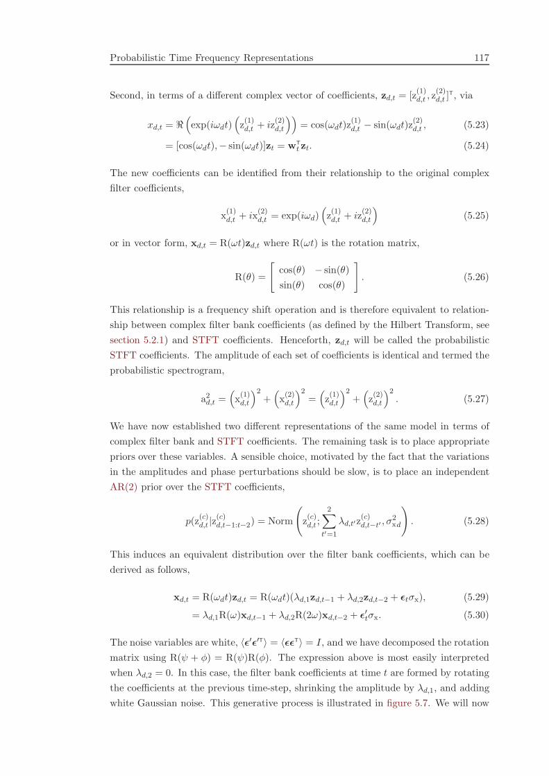
Probabilistic Time Frequency Representations 117
Second, in terms of a different complex vector of coefficients, zd,t = [z(1)d,t , z
(2)d,t ]
T, via
xd,t = ℜ(
exp(iωdt)(
z(1)d,t + iz
(2)d,t
))
= cos(ωdt)z(1)d,t − sin(ωdt)z
(2)d,t , (5.23)
= [cos(ωdt),− sin(ωdt)]zt = wT
t zt. (5.24)
The new coefficients can be identified from their relationship to the original complex
filter coefficients,
x(1)d,t + ix
(2)d,t = exp(iωd)
(
z(1)d,t + iz
(2)d,t
)
(5.25)
or in vector form, xd,t = R(ωt)zd,t where R(ωt) is the rotation matrix,
R(θ) =
[
cos(θ) − sin(θ)
sin(θ) cos(θ)
]
. (5.26)
This relationship is a frequency shift operation and is therefore equivalent to relation-
ship between complex filter bank coefficients (as defined by the Hilbert Transform, see
section 5.2.1) and STFT coefficients. Henceforth, zd,t will be called the probabilistic
STFT coefficients. The amplitude of each set of coefficients is identical and termed the
probabilistic spectrogram,
a2d,t =
(
x(1)d,t
)2+(
x(2)d,t
)2=(
z(1)d,t
)2+(
z(2)d,t
)2. (5.27)
We have now established two different representations of the same model in terms of
complex filter bank and STFT coefficients. The remaining task is to place appropriate
priors over these variables. A sensible choice, motivated by the fact that the variations
in the amplitudes and phase perturbations should be slow, is to place an independent
AR(2) prior over the STFT coefficients,
p(z(c)d,t |z
(c)d,t−1:t−2) = Norm
(
z(c)d,t ;
2∑
t′=1
λd,t′z(c)d,t−t′ , σ
2xd
)
. (5.28)
This induces an equivalent distribution over the filter bank coefficients, which can be
derived as follows,
xd,t = R(ωdt)zd,t = R(ωdt)(λd,1zd,t−1 + λd,2zd,t−2 + ǫtσx), (5.29)
= λd,1R(ω)xd,t−1 + λd,2R(2ω)xd,t−2 + ǫ′tσx. (5.30)
The noise variables are white, 〈ǫ′ǫ′T〉 = 〈ǫǫT〉 = I, and we have decomposed the rotation
matrix using R(ψ + φ) = R(ψ)R(φ). The expression above is most easily interpreted
when λd,2 = 0. In this case, the filter bank coefficients at time t are formed by rotating
the coefficients at the previous time-step, shrinking the amplitude by λd,1, and adding
white Gaussian noise. This generative process is illustrated in figure 5.7. We will now

Probabilistic Time Frequency Representations 118
x(2)d,t
x(1)d,t
z(2)d,t−1
z(1)d,t−1
z(2)d,t
z(1)d,t
xd,t−1
µd,t
Figure 5.7: Schematic illustrating the relationship between the probabilistic filterbank (x) and Short Time Fourier Transform coefficients (z). The parametersare chosen such that, λ1 = 1 and λ2 = 0. The filter bank coefficients are theprojections of a phasor which rotates around at a mean rate of ω, and undergoesslow perturbations. The STFT coefficients are the projections of the same phasor,but into a frame which rotates at a rate of ω with respect to that of the filter bankcoefficients. The rotating frame is illustrated in blue. The red circle indicates theprior distribution of the next coefficient, conditioned on the previous. The centreis µd,t = 〈xd,t|xd,t−1〉.
summarise the two versions of the model. First, the forward model for the filter bank
representation is,
p(xd,t|xd,t−1:t−2) = Norm(xd,t;λd,1R(ωd)xd,t−1 + λd,2R(2ωd)xd,t−2, σ2xdI), (5.31)
p(yt|x1:D,t) = Norm
(
yt;D∑
d=1
x(1)d,t , σ
2y
)
. (5.32)
When λd,1 = 1 and λd,2 = 0 this is corresponds to the Probabilistic Phase Vocoder
(Cemgil and Godsill, 2005a,b), so named because it is a probabilistic version of the
phase vocoder (Flanagan and Golden 1966 and see section 2.1.5.1). Exact inference
is possible using the Kalman Smoothing algorithm. Second, the STFT version of the
model is,
p(zd,t|zd,t−1:t−2) = Norm(zd,t;λd,1zd,t−1 + λd,2zd,t−2, σ2xdI), (5.33)
p(yt|z1:D,t) = Norm
(
yt;
D∑
d=1
(
cos(ωdt)z(1)d,t − sin(ωdt)z
(2)d,t
)
, σ2y
)
. (5.34)
Again, in the case where λd,1 = 1 and λd,2 = 0, this is an instance of the Bayesian Spec-
trum Estimation model proposed by Qi et al. (2002). This formally identifies Bayesian
Spectrum Estimation and the Probabilistic Phase Vocoder as different representations
of identical models. The former being a probabilistic form of STFT and the latter a

Probabilistic Time Frequency Representations 119
probabilistic form of filter bank, and the relationship being the usual frequency shift
operation.
Once again the Kalman Smoother can be employed to compute the moments of the
posterior distribution for these models. The implementational details are given in the
appendix in sections F.2.2 and F.2.3. The probabilistic filter bank and spectrogram
representations are illustrated on a short section of speech in figure 5.8 where they are
compared with the standard gammatone representation. The parameters of the model
were chosen by fitting the spectra of model’s components to that of a gammatone filter.
In order to carry out this fitting procedure, it is necessary to derive an analytic form
for the model filters. This is most simply done by noting that the auto-correlation of
the filter bank coefficients can be written in terms of the auto-correlation of the STFT
coefficients,
〈xd,txd,t+τ 〉 = wT
t 〈ztzT
t+τ 〉wt+τ = γAR(2)(τ) cos(ωτ). (5.35)
Therefore, the spectrum is equal to the convolution of the spectrum of a standard
AR(2) process, which was derived previously in equation (5.18), with a pair of delta
functions at ±ω. For completeness, we note that the marginal variance is equal to that
of the composite AR(2) process.
In both the Bayesian Spectrum Estimation and the Probabilistic Phase Vocoder the
parameters are set so that λ1,d = 1 and λ2,d = 0. This is a severe choice. First, be-
cause the corresponding filters are non-stationary (they have infinite marginal variance
assuming a finite initial value) and because in this limit the prior spectra are delta-
functions. Second, because it means that there is no correlation between successive
instantaneous frequencies, 〈φd,tφd,t−1〉 = σ2xd
1−λd,1
1+λd,1→ 0. In point of fact, it is usually
desirable for the instantaneous frequencies to be correlated through time so that the
sinusoid has a slowly-varying instantaneous frequency.
This section has described how Bayesian Spectrum Estimation and the Probabilistic
Phase Vocoder can be interpreted as models that represent signals in terms of time-
varying amplitudes and time-varying phases. This new perspective encourages rein-
terpretation of the prior distributions over coefficients, xt or zt, as distributions over
amplitude and phase. Although the distribution over coefficients is factored in these
models, the distribution over amplitude and phase is dependent. This is easy to see if
one contrasts what happens when the amplitude is very small (in which case the dis-
tribution over angles becomes uniform), to the case where the amplitude is very large,
(in which case the distribution over phases is very peaked around the previous phase
plus ω). In fact, the full joint distribution is
p(at, φt|at−1, φt−1) =at
2πσ2x
exp
(
− 1
2σ2x
(
a2t + λ2a2
t−1
)
+λ
σ2x
atat−1 cos(φt − φt−1 − ω)
)
,
(5.36)

Probabilistic Time Frequency Representations 120
chan
nel 3
chan
nel 2
chan
nel 1
0.05 0.1 0.15 0.2 0.25 0.3
time /s
y
0 100 200 300 400 500 600 700 800 900 1000
Frequency /Hz
Cha
nnel
Spe
ctra
Figure 5.8: Comparison of the probabilistic phasor and gammatone filter bankrepresentations of a speech sound. Top panel shows the spectra of the threechannels in the gammatone (black lines) and probabilistic phasor (red lines)filter banks. The properties of the gammatone filter bank were chosen usingGlasberg and Moore (1990). The parameters of the probabilistic phasor filter bankwere chosen to minimise the squared error-between the spectra of the gammatonefilters and the probabilistic filters. Inference proceeds via Kalman Filtering be-cause the gammatone filters are causal. The observation noise is set to σ2
y = 10−4.The lower left set of plots show the three filter outputs ordered from highestfrequency (top) to lowest (bottom). The overall scale of the gammatone filter ac-tivities (shown in blue) are arbitrary and so they have been set to the scale of theprobabilistic filter activities (shown in red). The lowest panel on the left showsthe sum of the filter activities above (red, identical to the input sound). The threeright hand panels shown the amplitudes of the filter coefficients. The amplitudesof the gammatone filters (blue) are derived using the Hilbert transform, and theamplitude of the probabilistic filters (red), formed using the expression in the text.The traditional amplitudes are much slower than their probabilistic counter-parts.This is partly because of the low setting of the observation noise in this example,and partly because of the shallow skirt of the probabilistic filters compared to thegammatone.
which is conditionally a uniform distribution when at−1 = 0 and a strongly peaked von
Mises distribution (Bishop, 2006) when at−1 is large. One of the features of this prior
then, is that the phase differences, φt = φt−φt−1 = ω+Φt−Φt−1, called instantaneous
frequencies, tend to have larger magnitudes when the amplitude is small. In fact the

Probabilistic Time Frequency Representations 121
instantaneous frequencies can become negative. This property may be undesirable and
so a target of future research should be to develop a tractable framework for using
decoupled priors p(φt, at|φt−1, at−1) = p(φt|φt−1)p(at|at−1) in which the positivity of
the instantaneous frequency is assured.
One important relationship for the traditional STFT is the so-called uncertainty prin-
ciple, which is an instance of the more general fact that a signal which is narrow in
time, is broad in frequency, and vice versa (Cohen, 1994). Thus, if a windowed signal is
narrow in time because the window is short, then its Fourier transform pair, the STFT,
will be broad in frequency. A similar relationship holds for the probabilistic version,
because the prior contribution is essentially a traditional STFT. Importantly, this re-
lationship has no connection with the uncertainty in the posterior distribution over
latent variables. Therefore, the slower the prior, the broader the temporal resolution,
but the narrower the bandwidth and the finer the frequency resolution. Conversely, the
faster the prior the higher the temporal resolution, but the wider the bandwidth and
the broader the frequency resolution. This trade-off is shown in figure 5.9. If the prior
and data are not well matched, then there will be a mis-match and the estimation will
be poor. The contribution from the likelihood complicates this relationship slightly,
but it holds on average.
The methods developed in this section are particularly suited to tasks which involve
missing data or resynthesis. An example of such a task which is practically relevant is
to modify the time-scale of speech. The naıve approach is to re-sample the signal whilst
retaining the original sample rate upon play-back. However, this modifies the frequency
content of the signal, as well as the duration. The methods developed here offer an
elegant alternative. The probabilistic spectrogram is re-sampled, and the probabilistic
filter bank coefficients are generated using the original frequency shift operation. The
data are then synthesised from these coefficients. As the frequency shift operation
is unaffected by the re-sampling, the frequency content of the signal remains largely
unaffected, but the time-scale of the sinusoidal activations, and therefore of the signal,
have been altered (see http://tinyurl.com/archivesounds for examples).
GPTFMs can also be used for missing data and denoising tasks. We defer experiments
of this kind until section 5.3.5 so that GPTFMs can be compared to the new, more
sophisticated, models developed in the next section.
5.2.3 Conclusion
The purpose of this section was to introduce probabilistic versions of time-frequency
representations. The probabilistic approach is natural, because the task of estimating
the sinusoidal content of a one-dimensional signal at each time point is an ill posed
problem. We focused on a family of models, called Gaussian Process Time-Frequency
Models, and provided a number of tractable representations in this class including

Probabilistic Time Frequency Representations 122
0.02 0.04 0.06 0.08 0.1 0.12 0.14−1
0
1
y
200
250
300
350
400
freq
uenc
y /H
z
200
250
300
350
400
0.02 0.04 0.06 0.08 0.1 0.12 0.14
200
250
300
350
400
time /s
Figure 5.9: The uncertainty relationship for the probabilistic spectrogram. Toppanel shows the signal which is a sinusoid whose frequency makes step changes each0.05s starting at 200Hz, then changing to 300Hz and finally to 400Hz. The threepanels below show probabilistic spectrograms with filter centre frequencies from170Hz to 450Hz. The bandwidths of the filters decrease from the top panel to thebottom panel. Practically this is achieved using the following parameter settings,λ1 = [0.96, 0.98, 0.995] and λ2 = 0. The broad filters resolve the switching pointsaccurately, but have poor frequency resolution (top panel). The narrow filters havesuperior frequency resolution, but poor temporal resolution. This is analogous tothe standard uncertainty relationship.
probabilistic versions of filter banks, the STFT and the spectrogram. These methods
are complementary to existing approaches to time-frequency analysis. On the one hand
traditional representations are computationally cheap to realise, but they have the
draw back that resynthesis is more complicated and often unprincipled. On the other
hand, the probabilistic representations are more time-consuming to realise because
inference is computationally demanding. However, the advantage is that resynthesis
is cheap and principled. There are other advantages too, like the ability to learn the
parameters of the time-frequency representation. Importantly, because these models
handle uncertainty, they are relatively simple to combine with models for the long-time
modulation content of sounds, which is the goal of the next section.

Multivariate Probabilistic Amplitude Demodulation 123
5.3 Multivariate Probabilistic Amplitude Demodulation
The main goal of this chapter is to develop a probabilistic model of sounds comprising a
sum of co-modulated coloured noise carriers called Multivariate Probabilistic Amplitude
Demodulation (M-PAD). The previous section has made an important step in this
direction which is to articulate a range of models for the fine-structure of natural sounds.
These models were Gaussian which meant inference was simple, but the explanatory
power was limited. In this section we return to our main focus, which is to use these
probabilistic time-frequency representations to model the carriers in natural sounds,
and to combine them with a model for the long-time and cross-channel modulation
structure. It will be shown that the resulting model is able to capture the statistics of
simple auditory textures like running water, wind, fire and rain, and it out-performs
GPTFM on missing data tasks.
5.3.1 The forward model
The forward model for M-PAD comprises a set of positive, slowly varying envelopes
(ad,t) which multiply a set of quickly varying real-valued, (positive and negative) carriers
(cd,t), which are summed, with some Gaussian noise, to produce the data (yt),
yt =
D∑
d=1
cd,tad,t + σyǫt (5.37)
The carrier processes will be auto-regressive Gaussian variables. Two possible choices
are AR(2) processes (see section 5.2.2.3),
p(cd,t|cd,t−1:t−2, θ) = Norm
(
cd,t;
2∑
t′=1
λd,t′cd,t−t′ , σ2d
)
, (5.38)
in which case the model will be called M-PAD(ARc), and probabilistic phasors (see
section 5.2.2.4),
cd,t = cos(ωdt)z(1)d,t − sin(ωdt)z
(2)d,t , z
(i)d,t = Norm
(
z(i)d,t;
2∑
t′=1
λd,t′z(i)d,t−t′ , σ
2d
)
, (5.39)
in which case the model will be termed M-PAD(ARφ).
In both versions of M-PAD, the envelope processes are formed from real-valued, in-
dependent processes – henceforth called the transformed envelopes (xd,t) – which are
linearly mixed, and then passed through a static, positive, non-linearity,
ad,t = a
(
E∑
e=1
gd,exe,t + µd
)
, e.g. a(x) = log(1 + exp(x)). (5.40)

Multivariate Probabilistic Amplitude Demodulation 124
In the following the transformed envelopes will be generated from zero-mean stationary
GPs. Half of the transformed envelopes (xe,1:T ) have associated observations, whilst
the other half do not have associate observations (xe,T+1:T ′ ), where T′
= 2(T −1). The
transformed envelopes are chosen to be locally correlated, so that they are slow, and to
lie on a ring, so that the FFT can be used to speed up computations (see section 3.2.2).
Therefore,
p(xe,1:T′ |Γe,1:T
′,1:T
′ ) = Norm(
xe,1:T′ ; 0,Γe,1:T
′,1:T
′
)
, (5.41)
where the covariance is stationary, Γe,t,t′ = γe,|t−t′|. That is, the covariance is a function
of the separation as measured around the ring.
One of the goals set out at the start of this chapter was to construct a generative
model in which inference and learning was able to discover a low dimensional and slowly
varying representation of the modulation structure. The generative process described
above does just that when the number of transformed envelopes is smaller than the
number of amplitudes, E < D. In this case, M-PAD will learn a low-dimensional
representation of the modulation structure in terms of a small number of slowly varying
transformed-envelopes, which control patterns of co-modulation in the signal.
This model for the amplitude modulation is motivated by the fact that the statis-
tics of modulation are carrier frequency-shift invariant (Attias and Schreiner 1997, see
section 2.2.1). M-PAD is additive (the sum of two M-PAD models is another M-PAD
model), which is important because it reflects the linear physics of sound generation.
In contrast, many probabilistic models for sounds containing a mixture of sources are
based on spectrographic representations of sounds and this turns a simple linear mixing
problem into a complex non-linear mixing problem (Roweis, 2004).
5.3.1.1 Relationship to other models
M-PAD has several important connections to existing models. Perhaps the simplest
relationship is that M-PAD reduces to a standard GPTFM when the envelopes are
fixed (e.g. to unity ad,t = 1). It is therefore representationally more powerful than this
model class, but it is more vulnerable to over-fitting. Importantly, this connection to
GPTFMs leads to an efficient inference scheme (described in the next section).
Another simple relationship is that M-PAD is equivalent to GP-PAD when there is one
transformed envelope, E = 1. In the next section, new inference procedures based on
the Kalman Smoother are derived for M-PAD, and consequently they can be used for
GP-PAD too. One benefit of the new schemes over those developed in chapter 3 is
that they are able to denoise data using a model containing a carrier which is coloured
noise.
M-PAD is a temporal generalisation of a Gaussian Scale Mixture (GSM) model in which

Multivariate Probabilistic Amplitude Demodulation 125
the Gaussian (carrier) variables are assumed to vary quickly through time, whilst the
scale (envelope) variables change more slowly. The generation of the scale variables, via
a linear mixture of Gaussian variables which are then positively transformed, is similar
to many current approaches (Wainwright and Simoncelli, 2000; Karklin and Lewicki,
2003, 2005). The generation of the low-level Gaussian variables is handled rather
differently, because it usually proceeds by passing white noise through a (spatial) filter.
Here the filters and the white-noise are effectively folded into one variable, the carriers,
whose prior dynamics specify the frequency content.
When the modulation weights are identity, G = I, M-PAD(ARφ), in which the carriers
are probabilistic phasors, is a model for signals containing amplitude modulated (noisy)
sinusoids. In this sense, it is a probabilistic version of sub-band demodulation (see
section 2.1.2). More general settings of the weights allow more complicated features
to be modelled like harmonic stacks and broad-band noise. In this setting M-PAD
is a probabilistic version of a sinusoidal analysis method, like the McAulay Quatieri
algorithm and the harmonic-plus-noise model (see section 2.1.3).
One of the ways of evaluating the success of M-PAD as a model for natural sounds is
to train the model parameters on a sound, and then generate a new synthetic version
from the forward model. By listening to the synthetic sound and comparing it to the
original we can determine which aspects of the sound have been accurately captured
and which have not, thereby highlighting deficiencies in the model (see section 5.3.5.1).
This process invites comparison to the state of the art method for generating synthetic
sounds, like auditory textures, from training data (McDermott et al., 2009). The ele-
gant work of McDermott et al. does not employ a generative model as such, but there
are similarities to the generative approach employed here. In the first stage, several
statistics are computed empirically from a training sound. These statistics include the
marginal distribution of the waveform, the marginal histograms of the filter coefficients
and the auto- and cross-correlation of the log-Hilbert envelopes of the filter coefficients.
In the second stage, these statistics serve as target statistics which the new synthetic
sound should match as closely as possible. The quality of the match is measured by
an objective-function and synthesis involves iteratively updating the synthetic sound
so that the objective-function, and therefore the quality of the match, increases. The
art in the method is in choosing the appropriate statistics, so that they capture the
important aspects of the training sound, and in choosing the objective-function so that
the derivatives necessary for the optimisation are computationally cheap to compute.
McDermott et al. show that the statistics mentioned above are sufficient for synthesis-
ing realistic sounding auditory textures like running water, wind, fire and rain. M-PAD
is similar in flavour to this work; similar statistics are captured by the model, although
this is handled rather differently by learning parameters in the model rather than via
matching empirical histograms. A parametric description is often more useful than an
empirical histogram because it is a more compact description. However, for the same
reason, it is considerably less flexible which may affect the quality of the synthesised

Multivariate Probabilistic Amplitude Demodulation 126
sounds. Furthermore, the learning step in M-PAD is longer and more complicated
than simply computing target statistics from the training sound, but the subsequent
generation step is much faster as it does not involve an optimisation over the signal.
One of the differences between this work and that of McDermott et al. (2009) is that
the generative approach studied here will be evaluated using tests which involve filling
in missing data. In principle, the method of McDermott et al. could be also extended
to missing-data problems, but this is yet to be investigated. In order to generalise
their methodology to these problems, the waveform in the missing regions must be
estimated by matching its statistics to target statistics. In addition, a constraint needs
to be added to ensure that the new sound waveform in the missing region matches
the waveform either side, but this is a relatively minor modification of the original
algorithm.
5.3.2 Inference
Exact inference in this model is analytically intractable because of the two types of
non-linearity; the non-linear coupling between the carriers and envelopes (a product),
and the non-linear generation of the envelopes from the transformed envelopes. In
order to side-step these non-linearities, approximations are required for inference. One
approach is to follow the scheme developed in chapter 3 for GP-PAD which is to find
the most probable transformed envelope, given the data,
XMAP = arg maxX
p(X|Y, θ) = arg maxX
log p(X,Y|θ). (5.42)
The log-joint, log p(X,Y|θ), is complicated because it involves an integral over the
carriers,
p(X,Y|θ) =
∫
dC p(X,C,Y|θ) = p(X|θ)∫
dC p(Y,C|X, θ). (5.43)
However, when the envelopes are fixed, the distribution over the carriers and the data is
Gaussian. In other words, p(Y,C|X, θ) is Gaussian in the carriers and so it is possible to
compute the integral exactly. A naıve approach would involve inversion of a DT ×DT
matrix which is computationally intractable, but the Kalman Smoother provides a
tractable recursive inversion method, being of order TD3 rather than (DT )3 ( Kalman
1960 and see section F.3.3). Further details for how to perform Kalman Smoothing in
this model are given in section F.3.1 in the appendices. The key is to identify a linear
Gaussian state-space model that is equivalent to M-PAD in the case where the envelopes
are fixed. This leads to a version of Kalman Smoothing in which the envelopes define
time-varying emission weights.
The fact that the objective function can be computed efficiently, suggests that its
gradients can also be computed efficiently. To show that this is the case, notice that

Multivariate Probabilistic Amplitude Demodulation 127
the derivative of the objective function with respect to the transformed envelopes can
be written as follows,
d
dxe,tlog p(X,Y|θ) =
d
dxe,tlog p(X|θ) +
1
p(Y|X, θ)
∫
dCd
dxe,tp(Y,C|X, θ). (5.44)
The first term is the derivative of the log-prior and this is simple to compute as it is
equivalent to the derivative of the prior in GP-PAD (see section F.3.1 in the appendix).
The second term also takes a simple form,
1
p(Y|X, θ)
∫
dCd
dxe,tp(Y,C|X, θ) =
1
σ2y
yt 〈cd,t〉 −∑
d′,t
ad′,t
⟨
cd,tcd′,t
⟩
dad,t
dxe,t(5.45)
where the averages, 〈•〉, are with respect to the posterior distribution over the carriers,
given the data and the envelopes, p(C|X,Y, θ). These sufficient statistics (the mean
and covariance of the carriers) are also returned by the Kalman Smoother and so the
gradients of the objective are also efficiently computable.
5.3.2.1 Relationship to other inference schemes
The scheme described in the previous section is identical to that used for GP-PAD
when D = E = 1. The use of the Kalman Smoother to compute the integration over
the carriers is an alternative to the approaches developed in chapter 3 and it can be
more powerful. For instance, the new method is able to perform denoising in models
with coloured-noise carriers which is computationally intractable using the previous
approaches. However, there is a price to pay for the generality of the new method,
which is the fact that for simpler models, like those with a white noise carrier or those
without observation noise, the methods developed in chapter 3 are significantly faster.
Inference in non-temporal GSM models typically proceeds by joint MAP estimation of
the carrier and envelope variables (Karklin and Lewicki 2003, 2005 and see
section 2.2.2.1). This procedure is fraught with difficulties due to over-fitting, and so
the approach here, in which the carriers are integrated out, is superior. More recently,
models have been developed that are related to GSM models in which the carriers have
been integrated out (e.g. Karklin and Lewicki 2008) and so they are less susceptible
to over-fitting. Of course, M-PAD differs substantially from these models because it is
fully temporal.
One alternative method for inference in M-PAD is to use a structural variational free-
energy approach (Jordan et al., 1999; Wainwright and Jordan, 2008) that approximates
the posterior distribution as being factored between carriers and transformed envelopes,
p(C,X|Y, θ) ≈ q(C)q(X). (5.46)

Multivariate Probabilistic Amplitude Demodulation 128
This factorisation side-steps the analytic intractability arising from the non-linear prod-
uct between the carriers and the envelopes, but a further approximation is required to
handle the non-linear prior over envelopes. A natural choice is to restrict the distri-
bution over the transformed envelopes to be a delta function, q(X) = δ(X − X0). In
the variational approach, the distribution over the carriers and envelopes are chosen by
minimising the free-energy,
F(q(C),X0, θ) = 〈log p(Y,C,X0|θ)〉q(C) + H(q(C)), (5.47)
= log p(Y,X0|θ) − KL(q(C)||p(C|X0,Y, θ)). (5.48)
Therefore, the optimal variational update for the carriers is equal to the true posterior
distribution of the carriers given the data and the envelopes,
q(C) = p(C|Y,X0, θ). (5.49)
The optimal distribution over the envelopes is found by optimising the Free-Energy, or
equivalently,
X0 = arg maxX
〈log p(Y,C,X|θ)〉q(C) (5.50)
Standard variational inference for the carriers and the envelopes can be carried out
by alternating the updates given by equation (5.49) and equation (5.50), which is the
variational Expectation Maximisation (EM) algorithm. The expression for the Free-
Energy after a carrier update takes a simple form,
F(q(C),X0, θ) =
∫
dC q(C) logp(X0,C,Y|θ)
q(C)= log p(X0,Y|θ). (5.51)
That is, after each carrier update, the free-energy is equal to the true log-joint of
the carriers and transformed envelopes. In other words, the variational EM algorithm
will converge to the MAP transformed envelopes, X0 = XMAP. Therefore, it finds an
identical solution to the method introduced in the last section. In practice, although
the variational EM algorithm will converge to the same solution eventually, it performs
catastrophically because the carriers and transformed envelopes are strongly coupled
(by explaining away) and so co-ordinate ascent takes only small steps. The approach
described in the previous section converges much more quickly as it is equivalent to
direct gradient ascent on the Free-Energy. From this perspective, the learning algorithm
described in the last section is an extension of the Expectation Conjugate Gradient
method (Salakhutdinov et al., 2003) to the variational setting.
One of the problems with the MAP approach proposed in the last section, is that
it has a cubic dependence on the number of carriers (D). The connection to varia-
tional methods offers a potential method for reducing this computational complexity
by the use of more severe factorial approximations to the posterior. For instance, the

Multivariate Probabilistic Amplitude Demodulation 129
mean-field approximation, q(C) =∏
d,t q(cd,t), reduces the computational cost of the
updates for the carriers to linear in their number, TD. However, although this does
speed up the E-Step appreciably, it suffers from severe biases. The biases arise be-
cause the mean-field approximation is at its tightest when there are no correlations
between the carriers in the posterior, because the KL term is zero in this regime as
can be seen from equation (5.48). This causes the peaks in the free-energy to be bi-
ased away from maxima in the likelihood toward regions where the bound is tightest.
The result is that components are aggressively pruned out in the mean-field solution
so that just one is active at each time-point (i.e. one envelope has a high value at each
time point), thereby removing all of the correlations in the posterior. This is a typical
example of the compactness property inherent in variational methods (MacKay, 2003;
Wang and Titterington, 2004; Turner and Sahani, in press).
A limitation of the MAP estimate described in the last section is that it does not
return estimates of the uncertainty in the estimated envelopes. A possible extension
is to sample the envelopes using an Monte Carlo Markov Chain (MCMC) method,
like Hamiltonian Monte Carlo (MacKay, 2003). In this setting the exact integration
over the carriers is a Rao-Blackwellisation step (Casella and Robert, 1996). The main
problem with a sampling approach is that, roughly speaking, each sample will take as
much time to be generated as the MAP estimate. For many applications, the MAP
estimate might take as many as 5 hours to compute, and so even a small amount of
samples would result in a prohibitive increase in computer-time.
5.3.3 Learning
Parameter learning in M-PAD is made difficult by the same over-fitting problems en-
countered in GP-PAD (see section 3.2.5). These problems are compounded by the fact
that M-PAD contains a much larger number of latent variables (and so approximate
integration is even harder) and a much larger number of parameters (and so searching
for the best parameters is much more time consuming). As a result heuristic methods
are required to learn the parameters which are based on the analysis described at the
start of this chapter. However, the development of these heuristic methods benefits
greatly by considering more principled approaches from the probabilistic framework.
The set of parameters in the model includes the carrier marginal variances and dynamics
(i.e. the typical frequency content), the transformed envelope means and marginal
variances (which control the depth and skew of the modulation in each sub-band), the
time-scale of the transformed envelopes, and the weights (which control the cross sub-
band patterns of modulation). We will now consider each of these parameters in turn for
the version of M-PAD which uses AR(2) processes to model the carriers, M-PAD(ARc).
The approach will be to first learn the parameters of a model containing independent
modulators (G = I) and then use this to bootstrap learning in the full model.

Multivariate Probabilistic Amplitude Demodulation 130
First, we consider learning the centre-frequencies and bandwidths of the carriers via
the parameters, λ1,d, λ2,d, σ2dD
d=1. A simple and expedient option is to fix the filter
properties so that they form a normal probabilistic filter-bank e.g. so that the centre-
frequencies and bandwidths match those of a gammatone filter bank. This approach
leads to a versatile representation, but often it cannot synthesise realistic sounding
stimuli e.g. when there are narrow spectral components in the signal at high frequencies.
Alternatively, the filter centre-frequencies and bandwidths can be learned directly from
the data. A sensible heuristic procedure is to fix the envelopes in M-PAD to unity,
ad,t = 1, and then fit the spectrum of the data using equation (5.15). The assumption is
that the addition of slow modulators into the model does not greatly alter the spectrum
as they have the effect of broadening the spectral content slightly. Of course, if the
modulation has a fast time-scale then this heuristic fails and so it is important to
verify that the procedure has worked retrospectively by sampling from the model and
comparing the synthetic spectrum to that of the original signal.
The next set of parameters that will be learned are the means and marginal vari-
ances of the transformed envelopes, µe, σ2eE
e=1. A heuristic approach, motivated by
McDermott et al. (2009), is to pass the sound through the probabilistic filter bank,
again using ad,t = 1, and to fit the mean and the marginal variance of the transformed
envelopes using the marginal distribution of the output of each filter. The assumption
is that the filtering step has identified a single carrier-modulator pair, yd,t ≈ ad,tcd,t,
and so the techniques developed for learning these parameters in GP-PAD can be used
(see section 3.2.5.1). Once the mean and the marginal variance of the transformed
envelopes has been learned, GP-PAD can also be used to learn the time-scale of the
modulation.
The procedures described up to now are sufficient for learning all of the parameters in
M-PAD when each of the carriers undergoes independent modulation, D = E and G =
I. The final step is to use this model to bootstrap learning in a model with dependent
modulation and where D 6= E. The approach begins by inferring the transformed
envelopes for the complete model using the methods developed in the last section.
When the envelopes have converged, the modulation weights can be initialised using a
heuristic procedure based on the one described at the start of this chapter in section 5.1.
First, PCA is used to reduce the dimensionality of the transformed envelopes. A typical
criterion is that 95% of the variance in the data should be retained. SFA is then used
to find the directions of the transformed envelopes within the PCA space. This yields a
set of weights, G, and a new set of transformed envelopes. The means and the variances
of the new transformed envelopes must also be determined and a sensible heuristic is
to choose them so that the marginal statistics in each sub-band of the model are as

Multivariate Probabilistic Amplitude Demodulation 131
similar as possible after the dimensionality reduction. That is,
µold,d ≈E∑
e=1
gd,eµnew,e and σ2old,d ≈
E∑
e=1
g2d,eσ
2new,e. (5.52)
The final step is to refine the modulation weights (and the transformed envelopes) by
optimising the joint distribution of the data and the transformed-envelopes,
G∗,X∗ = arg maxG,X
log p(Y,X|G, θ). (5.53)
An unconstrained optimisation of the weights leads to an over-fitting problem whereby
the norm of the transformed envelopes shrinks to zero, whilst the norm of the weights
diverges to infinity. This means the norm of the weights has to be constrained to avoid
over-fitting, and one choice is,∑D
d=1 g2d,e = 1, as is common practice when learning
parameters in ICA, sparse coding and GSMs.
The entire learning and inference process has a computational complexity which scales
roughly as, α1D2T+α2KT log(T ), where α1 and α2 are constants. Processing 2 seconds
of sounds with D = K = 30 and Fsamp = 16000Hz takes about 2 days.
5.3.4 Testing Learning and Inference in M-PAD(ARc)
The inference and learning scheme described in the previous section is heuristic and
so it is very important to determine whether it is reliable. In order to carry out such
a validation, the methods must be tested on synthetic data where ground truth is
known. The first test was to train the model on white noise, in which case the result
of inference and learning was a set of nearly constant modulator variables, with very
long associated time-scales and very small variances. This result indicates that the
modulation component of the model has been pruned correctly. The second testing
approach was more complicated and it used synthetic data generated from a model
containing D = 7 pure tone carriers (frequencies linearly spaced between 300−3000Hz),
which were modulated by E ≤ 7 GP transformed-modulators (time-scales linearly
spaced in time between 30 − 70ms, or 14 − 34Hz). The modulator weights in the
model, G, were normalised and orthogonal, but otherwise they were chosen so that
they pointed in random directions. The model settings – like the separation of the
time-scales of the components, and the use of sinusoidal carriers – were chosen so that
inference and learning are at least possible in principle.
The tests consisted of 35 simulations, made up of 5 different realisation from each
of the 7 different models (E = 1 − 7). The tests were completely blind in that all
the parameters in the model were learned from the data. The centre-frequencies of
the filters are simple to infer, because the data contains spectral peaks at the carrier
frequencies, but the properties of the envelopes are harder to learn. The results of

Multivariate Probabilistic Amplitude Demodulation 132
learning are summarised in figure 5.10. With regard to learning the cross-frequency
modulation, M-PAD usually learns the correct dimensionality of the model, although
there is a tendency to under-estimate when there are large numbers of modulators
(figure 5.10 panel A). On average, two or three of the true weight directions are found
(figure 5.10 panel C), but although the remaining inferred weights do not lie in the
direction of the true weights, they tend to span the true sub-space (figure 5.10 panel
B). Finally, the maximum error in the inferred length-scales is ten percent, which
is reasonably small, but this error grows with the number of modulators estimated
(figure 5.10 panel D).
The conclusion from these experiments is that the learning and inference procedures
developed for M-PAD are reasonably accurate for synthetic data. In the next section
they are applied to natural signals where their success can be qualitatively measured
by the quality of the sounds generated from the forward model and quantitatively
measured in missing data tasks.
1 2 3 4 5 6 70
1
2
3
4
5
6
7A
KIN
F
K1 2 3 4 5 6 7
−1
0
1
2
3
4
5
6
7C
num
ber
of w
eigh
ts fo
und
K1 2 3 4 5 6 7
0
1
2
3
4
5
6
7B
sub−
spac
e ov
erla
p
K1 2 3 4 5 6 7
0
2
4
6
8
10
12
14
16D
% ti
me−
scal
e er
ror
K
Figure 5.10: Testing learning and inference in M-PAD. The figure shows variousmeasures of the success of learning. Panel A shows the mean inferred dimension-ality as a function of the true dimensionality. Panel B shows the average numberof learned weights that lie in the true sub-space. A weight was considered to liein the true sub-space if the projection into that sub-space retained 98% of themagnitude of the vector. Panel C shows the number of inferred weights that pointin a direction within 10 degrees of a true weight. Panel D shows the average per-centage error in the inferred time-scales of the modulator. The shaded regions onall plots are the one standard deviation error-bars.
5.3.5 Results
In this section M-PAD(ARc) is applied to two separate tasks. In the first task the
model is trained on a variety of natural sounds, like running water, wind, fire, rain,
and speech sounds. Then, synthetic versions of these sounds are generated using the

Multivariate Probabilistic Amplitude Demodulation 133
parameters learned from these signals. The aspects of signals which M-PAD can and
cannot capture are then determined by comparing the original and generated sounds.
The conclusion is that M-PAD is able to accurately reproduce some auditory textures,
like running water, wind, fire and rain, but it struggles to capture signals with more
complex structure such as the asymmetric transients and frequency modulation that
occur in bird song and speech.
In the second task, the M-PAD(ARc) is trained on a speech sound and then it is
used to fill in missing sections of a new test sound uttered by the same speaker. The
performance of the model is compared to other models including, Bayesian Spectrum
Estimation (equivalently the Probabilistic Phase Vocoder) and an AR(2) filter bank
which was trained on the same sound. The results indicate that M-PAD(ARc) signif-
icantly outperforms these algorithms by at least 6dB on gaps of an intermediate size
(5-30ms).
5.3.5.1 Generation of synthetic sounds
The first and simplest way of evaluating M-PAD is to train the model parameters
using a range of different signals and then to generate synthetic versions from the
generative model. The results of this procedure, which can be found in the sound
archive (http://tinyurl.com/archivesounds) indicate the aspects of natural sounds
which the model is able to capture and the aspects which it is not. This section
begins by considering simple stimuli, which the model captures successfully, and ends
with complex stimuli, which the model cannot fully capture. The conclusion is that
the model is capable of synthesising a large number of realistic sounding auditory
textures, including wind, running water, fire and falling rain drops, although it does
fail to capture some aspects of these stimuli. However, it is not capable of synthesising
realistic sounding complex animal vocalisations like bird song and speech. Importantly,
the results reveal the characteristic statistics of each of these sounds which is one of
the main goals of the thesis.
Three different models were trained on each of the sounds considered in this section. In
order of complexity, the models were: An AR(2) filter bank; a version of M-PAD with
independent modulators (G = I); and a full version of M-PAD. Each model contained
D = 30 carrier components and the parameters were learned using the methods de-
scribed in this chapter. Samples from each of these models can be found in the archive
(http://tinyurl.com/archivesounds).
We begin by considering a running water sound and the experiments indicate that it
can be well captured by a model containing band-pass carriers which undergo indepen-
dent modulation. Critically, the statistical modulation depth of each modulator must
be large (we find µSto = 0.77 ± 0.17) so that the generated data is kurtotic. Moreover,
the modulation time-scale must be quite short (roughly 2 − 10ms). This conclusion

Multivariate Probabilistic Amplitude Demodulation 134
is supported by three pieces of evidence. The first is that the version of M-PAD with
independent modulators is able to produce realistic sounding running water textures.
The second piece of evidence is that the AR(2) filter bank is not capable of synthesising
realistic sounding versions, which indicates that the addition of independent modula-
tors to the model is critical. The third piece of evidence is that when the full version
of M-PAD is trained on the running water sound, the model retains a full set of com-
ponents, D = E, and it discovers local weights, Gd,e ≈ 0 ∀ d 6= e. That is, it is of
the same form as the independent model. The general finding that water sounds are
characterised by independently modulated band-pass carriers, with a short time-scale
of modulation and large modulation depth, was supported by repeating the analysis on
a second running water sound (for which we find similar statistical modulation depths
of µSto = 0.60 ± 0.33 and time-scales from 5 − 20ms).
Although M-PAD is able to produce synthetic auditory textures which are recognisable
as running water sounds, the synthetic sounds do not sound like samples recorded from
exactly the same source in exactly the same way. There are many potential reasons for
this observation, but two of the most likely are that there are either biases in the learning
procedures or that there are deficiencies in the model that mean it cannot capture all of
the relevant statistics. With regard to biases in the learning process; these are almost
inevitable given its ad hoc nature. In a sense, it is surprising that the synthetic sounds
appear as similar to the training sounds as they do. With regard to deficiencies in the
model, we will certainly encounter sounds which are characterised by statistics which
the model cannot capture (e.g. animal vocalisations which have asymmetric onsets and
offsets and frequency sweeps). However, at least in the case of the running water sounds,
the first explanation appears the more likely. In particular, the generated sounds can
often be made to sound more like the original sound by increasing the sparsity of the
modulators (e.g. by increasing µd). This indicates that there are biases and that they
are important perceptually, but it cannot rule out the possibility that these, or other,
water sounds contain statistical regularities which cannot be captured by the model.
The next sound under consideration is a wind texture, the analysis of which proceeded
as for the running water sound. The sample from an AR(2) filter bank captures the
short-time structure of the original sound, but it lacks the long-time fluctuations. The
sample from the version of M-PAD with independent modulation is rather better be-
cause it has long-time modulation structure. However, the sample from the full model
sounds better still, indicating that wind is best captured by comodulated carriers. In
fact, the full model is dominated by only three patterns of comodulation that have very
long time-scales (300ms - 2s) (the remaining components making a much smaller con-
tribution) and large statistical modulation depths (1.5-1.3). This indicates that wind
is well captured by a set of band-pass carriers which undergo a relatively small number
of patterns of comodulation that vary over a long time-scale.
The next texture under consideration is a fire sound. The fire sound is an impor-

Multivariate Probabilistic Amplitude Demodulation 135
tant example because it contains crackles, which are short transients, and it is unclear
whether M-PAD will be able to model this aspect of natural sounds a priori. The
crackles require simultaneous activation of carriers with a range of different centre
frequencies and so neither the AR(2) filter bank nor the version of M-PAD with in-
dependent modulators is able to reproduce fire-like sounds. However, the full model
is more successful. The crackles are handled by a single component with a very large
variance (twenty times that of the next largest component) and a very short time-scale
(1.3ms). The component’s weight vector is a high-pass function which strongly acti-
vates all of the carriers with centre frequencies from 3000 to 12000Hz. The remaining
components handle the slower aspects of the sound, like the background roar. The
synthetic sound is recognisable as a fire sound, but has quite a different quality from
the original. Unlike the auditory textures discussed previously, it is likely that part of
the problem is that the model is not able to capture all of the important statistics in the
original waveform. One piece of evidence that speaks to this issue is that the original
fire sound is heard differently when played in reverse. This is due to the asymmetric
pulse-resonance of the crackles (a quick excitation followed by a relatively slow decay).
Consequently, the important statistics of the fire sound are not invariant to a reversal of
time. M-PAD cannot capture this aspect of the data because its statistics are invariant
to time-reversal. Nevertheless, the synthetic texture is still recognisable as fire.
The final auditory texture that we will consider in this section is that produced by
rain drops falling onto a surface. Once again, this auditory texture contains transients
produced by the impact of the water droplets and so the full M-PAD model is required
to generate realistic sounding synthetic versions. Similar to the fire sound, a pair
of components, with much higher variances roughly ten times larger than any of the
other components, and shorter time-scales (1.7ms), model these transients. Again the
synthetic sound is recognisable as rain, but it has a different quality from the original.
The asymmetric pulse-resonance that results when the rain drops hit the surface is
likely to be the cause.
The fact that the model can capture some of the transients in auditory textures means
that it might be able to reproduce more general transient sounds, like those produced
from snapping twigs. Once again the asymmetries in these sounds mean that the
model cannot capture the statistics precisely. For example, the synthetic version of the
‘snapping twigs’ sound resembles the sound produced by scraping a stone. Nevertheless,
this does indicate that the model can produce sounds which resemble natural transients.
Interestingly, sounds generated from an independent version of M-PAD trained on this
sound are heard as water-like.
The final two sounds that we will consider in this section are bird song and speech.
These sounds are considerably more complicated than those considered previously and
so it is not surprising that the models cannot generate realistic sounding synthetic ver-
sions. Taking the bird song first, there appear to be three separate problems. The first

Multivariate Probabilistic Amplitude Demodulation 136
problem is that the AR(2) carrier processes are not as effective at modelling harmonic
sounds as they are at modelling ambient sounds, because they have broad skirts (see
section 5.2.2.3). This often means the generated version of sounds is more noisy than
the original, but it is particularly apparent for sounds with narrow spectral peaks. The
second problem is that the bird song contains frequency sweeps and the generative
model cannot capture structure of this sort. The third problem is that bird song con-
tains multiple time-scales of modulation, similar to phoneme and sentence time-scale
structure in speech, and a model containing modulators with a single time-scale variable
cannot replicate this.
Finally, we consider speech. Of all the models, the full version of M-PAD produces the
most realistic synthetic speech sound. However, it is a rather poor imitation. Surpris-
ingly, the model uses only a few modulation features (E ≈ 5) to capture the statistics
of the sound, pruning out the additional components. Each of the features sound like a
primitive phoneme. Most of the primitive phonemes model the periodic vowel sounds
and the remaining one or two model the noisy consonants (e.g. see figure 5.11). The
components lack the fine details of real phonemes, as can be demonstrated by listening
to them individually, presumably because they must be more general purpose.
−0.2
0
0.2
0.4
0.6
Gd,
1
−0.5
0
0.5
1
Gd,
3
250 500 1000 2000−0.5
0
0.5
1
frequency /Hz
Gd,
5
−5
0
5
−5
0
5
0 0.2 0.4 0.6 0.8 1 1.2 1.4 1.6
−5
0
5
time /s
Can y ou juice i t t oday p lease
Figure 5.11: M-PAD applied to a speech sound. The figure shows three ofthe five components learned from a speech sound. The components can also befound in the sound archive (http://tinyurl.com/archivesounds). The left handcolumn of the figure shows the component weights, g1:D,e, and the right handcolumn of the figure shows the contribution of that component to the waveform,ye,t =
∑Dd=1 cd,ta (gd,exe,t + µd) (red). The original waveform is shown in black for
comparison. The first two components (g1:D,1 and g1:D,3), shown in the top tworows, predominantly model different sorts of periodic vowels. The last component(g1:D,5), shown in the bottom row, predominantly models the noisy consonants.
The results in this section indicate that when M-PAD is trained upon basic auditory

Multivariate Probabilistic Amplitude Demodulation 137
textures including running water, wind, fire, and rain, it can produce recognisable
synthetic versions. The learning procedures appear to be biased because although they
are sufficient for generating textures which are perceived as being of the same class
as the original, they are not perceptually identical. Nevertheless, the implication is
that some of the most important statistics of auditory textures are those captured by
M-PAD, that is; the power in each sub-band of the signal, the modulation time-scale,
depth and skew, in each sub-band, and the patterns of modulation across sub-bands.
One additional feature of relevance to textures and their perception are asymmetric
transients, but this cannot be captured by M-PAD because the statistics of the model
are invariant to a time reversal. This limits the quality of the synthetic fire and rain
sounds the model can produce, but it does not appear to be of major perceptual
importance for these sounds. However, this and other deficiencies in the model, do
prevent M-PAD from synthesising realistic sounding animal vocalisations. Perhaps
the most important limitation of the model in this regard is the fact that the AR(2)
processes used to model the carriers have shallow skirts. Although this property of the
model appears to be useful when modelling auditory textures, it causes problems when
modelling harmonic sounds.
5.3.5.2 Filling in missing data
In the previous section M-PAD was trained on a variety of sounds including series of
spoken sentences. In this section we demonstrate the power of the model by using it
to fill in missing sections of a new speech sound uttered by the same speaker. The
purpose is to demonstrate that M-PAD provides more accurate estimates for the miss-
ing regions and therefore that it is a superior model. The performance of M-PAD is
compared with several other probabilistic models that include: a version of M-PAD
that is also trained on the original speech sound, but which contains independent mod-
ulation (D = E, G = I); an AR(2) filter bank whose filter properties have been trained
on the original speech sound; and Bayesian Spectrum Estimation (equivalently, the
Probabilistic Phase Vocoder), which is a general purpose method with no free param-
eters. The results can be seen in figures 5.12 and 5.13 and all of the stimuli used
in these experiments, together with the reconstructions can be found in the archive
(http://tinyurl.com/archivesounds).
When the missing sections of data are very short, all of the algorithms perform well be-
cause the task is very easy. In contrast, when the length of the missing sections is very
long, all of the algorithms perform poorly because their estimates decay to the mean
of the models’ priors which lie at zero. Therefore, the region of interest is the interme-
diate range of gap sizes between 5ms and 30ms. Here, Bayesian Spectrum Estimation
provides the worst estimates. This is unsurprising as it is a general purpose method,
developed to handle spectral estimation of unevenly sampled data, not to denoise or
fill in missing data. It is the extreme setting of the prior parameter settings that is

Multivariate Probabilistic Amplitude Demodulation 138
the source of the problems (as described in section 5.2.2.4). The AR(2) filter bank is a
very similar model to Bayesian Spectrum Estimation, but because its prior parameters
have been learned from a similar training speech sound, it performs significantly bet-
ter (by ≈ 15 − 25dB). The version of M-PAD with independent modulators is better
still, but the best method is the version of M-PAD with dependent modulators. This
outperforms the AR(2) filter bank by 5 − 7dB. The performance gain comes from the
fact that whereas the AR(2) filter bank fills in missing data using prior knowledge of
the long-time power spectrum of the signal, M-PAD effectively uses knowledge of the
local power spectra, e.g. of the current phoneme.
−5
0
5
MP
AD
−5
0
5
MP
AD
− In
d
−5
0
5
AR
(2)
lear
ned
0 10 20 30
−5
0
5
BS
E/D
HM
time /ms
−2−1
012
−2−1
012
−2−1
012
0 10 20 30
−2−1
012
time /ms
−2
−1
0
1
2
−2
−1
0
1
2
−2
−1
0
1
2
0 10 20 30
−2
−1
0
1
2
time /ms
Figure 5.12: Typical results for filling in missing sections of speech using proba-bilistic models. M-PAD and an AR(2) filter bank were trained on a speech sound.Then a new testing sound, from the same speaker and shown in black above, wastaken and short sections 15.625ms in duration were removed from the central por-tion of each phoneme. The missing portions are indicated by the grey region. Theprobabilistic models were used to fill in the missing sections (shown in red). Thetop row of plots shows M-PAD with dependent modulators and the second rowwith independent modulators. The second row from the bottom shows the AR(2)filter bank and bottom row is Bayesian Spectrum Estimation.
The results in this section show that M-PAD improves noticeably upon more simple
models. This indicates that it is capturing statistics of relevance in the speech sound,
and that the inference and learning procedures are not over-fitting.

Conclusions and Future Directions 139
0 5 10 15 20 25 30 35 40−10
−5
0
5
10
15
20
25
30
gap length /ms
SN
R /d
B
BSE/DHMAR2MPAD IndependentMPAD Dependent
Figure 5.13: A summary of the results of filling in missing sections of speechusing probabilistic models. Various probabilistic models were used to fill in missingsections of a speech sound (for full details see the text and figure 5.12). The qualityof the inferences was measured using the SNR (in decibels) and this is plottedas a function of the duration of the missing sections. M-PAD with dependentmodulation is the best model (shown in red), the use of independent modulationcauses the performance to drop by about 5dB (shown in magenta). The AR(2)filter bank (shown in blue) is worse still, but it significantly out-performs BayesianSpectrum Estimation (shown in cyan).
5.4 Conclusions and Future Directions
The goal of this chapter was to develop a probabilistic model for natural scenes that
combined a time-frequency and modulation analysis. The first step toward this goal
was to develop a framework for probabilistic time-frequency analysis. We provided
practical probabilistic versions of filter banks and the spectrogram based on linear
Gaussian state space models. The next step was to use the probabilistic time-frequency
model as a model for the carriers in natural sounds and to combine it with a model
for the modulators. This new model, called M-PAD, is a generalisation of PAD and
GSMs. We introduced an efficient MAP inference procedure, based on the Kalman
Smoother, and an ad hoc learning procedure. When M-PAD was trained on natural
auditory textures, it was able to synthesise realistic sounding versions of running water,
wind, fire and rain. However, it was unable to produce realistic versions of transient
sounds and animal vocalisations. However, M-PAD was able to fill in missing sections
of speech up to 30ms long, improving significantly on a pure probabilistic filter bank
model. This shows that although M-PAD cannot capture all of the relevant statistics
in speech, it is capturing some of the important features.
The results in this chapter indicate that the important statistics of auditory textures
are the power in each sub-band, the modulation time-scale, depth and skew, and the
patterns of modulation across sub-bands. Furthermore, they suggest that such statis-
tical representations could underlie sound texture perception, and that the auditory
system may use fairly simple statistics to recognise many natural sound textures. This

Conclusions and Future Directions 140
idea is explored further in chapter 6 in a more general auditory scene analysis context.
It is hoped that the tools developed in this chapter will prove useful to experimentalists.
For example, many studies into auditory processing would like to use natural sounds
as stimuli. However, they are often too complex and uncontrolled for this purpose. As
an alternative, tones and noise are employed because they are simple and controlled.
However, their simplicity often limits the conclusions. The methods in this chapter
offer a new way to produce stimuli in the mid-range, which are both natural sounding
and controlled, by generating auditory textures from a parametric model.
There are many opportunities for further work. Perhaps the most pressing issue is to
develop faster inference and learning implementations that can reduce the time taken
to model sounds (typically inference and learning will take several days for a signal
just a few seconds in duration). Another important goal should be to develop a more
principled learning procedure. In addition, many improvements can be made to the
model. One of the most important issues is to improve the model of the carriers so that
harmonic sounds can be captured. Another direction is to investigate models for the
transients in sounds, and in particular their asymmetric pulse resonance structure. One
idea is to use a version of Smith and Lewicki’s model for the carriers (Smith and Lewicki
2005, 2006, a review of which can be found in section 2.2.2.4), but this complicates in-
ference and learning. Alternatively, a model for the envelopes could be developed which
enabled them to be asymmetric. Another way of extending the current model is to in-
troduce binary latent variables to model the fact that sources can appear and disappear
throughout a signal. A version of this model connects to the MQ algorithm because
it contains a variable number of active sinusoids at each time-point (see Berkes et al.
in press for a model of a similar flavour). A final generalisation to the model would
incorporate multiple time-scales of modulation via cascades (see chapter 4). It is likely
that a generalisation of this sort is required to model speech and bird song. Techni-
cally, the new model for the amplitudes might incorporate a tensor product between
the amplitudes at the different levels,
ad,t =∑
k,k′
Wd,k,k′a(1)k,ta
(2)k′,t. (5.54)
The tensor contains a large number of parameters (D × K1 × K2) and so a reduced
rank approximation is likely to be required inorder to render learning tractable.

Chapter 6
Primitive Auditory Scene
Analysis as Inference
In this thesis, we have argued that the important low level statistics of natural sounds
are those relating to patterns of comodulation in the sub-bands of the signal. A genera-
tive model has been developed to account for these statistics which comprises a sum of
amplitude co-modulated coloured noise carrier processes. In the generative framework,
the carriers and the envelopes are treated as latent variables, which can be inferred
from a natural sound. This inference process has several interesting properties. For
instance, when the input stimulus is a tone which has had its middle section deleted
and replaced by noise, the tone is inferred by the model as continuing through the noise.
This happens in spite of the fact that the tone is absent in this region. Interestingly,
if we listen to this stimulus, the tone is heard to continue through the noise. This
is known as the continuity illusion. This connection suggests that other perceptual
results might also correspond to inference in this generative model. In fact, it will be
demonstrated in this chapter that many of the basic principles which listeners appear
to use to understand simple stimuli, are consistent with the idea of primitive auditory
scene analysis as inference.
This chapter is organised as follows: It begins with a review of primitive auditory
scene analysis that describes the most basic principles which the auditory system uses
to analyse sounds. These results constrain the form of a suitable generative model for
primitive auditory scene analysis, and we argue that a subset of the models developed in
chapter 5 fulfil these constraints. We then provide specific, simplified examples, where
inference qualitatively replicates the basic principles believed to underpin primitive
auditory scene analysis.

Primitive Auditory Scene Analysis 142
6.1 Primitive Auditory Scene Analysis
The first stage of auditory processing is relatively well understood physiologically and
that is to convert the incoming sound into a time-frequency representation
(Patterson et al., 1988; Moore, 2003). This reveals the local energy in a frequency
band at a particular time. In subsequent stages, psychophysical evidence suggests that
primitive grouping principles are used to associate local regions of spectral-temporal
energy arising from a common source (Bregman, 1994; Darwin and Carlyon, 1995).
Common sense would suggest that the spatial location of the source would be the most
powerful principle upon which to base this grouping. However, the cues for spatial
location – inter-aural delay and level differences, and spectral cues – are often com-
plicated by reverberation, echoes, the presence of multiple-sources, and the fact that
sounds refract around intermediate objects. The result is that the auditory system is
not as reliant on the cues for spatial location as might be expected. For example, a
monophonic radio play can be easily understood even though all sounds come from the
same spatial location. Moreover, if cues for spatial location are placed in tension with
other grouping cues (like the fact that sounds with a common fundamental are grouped
together) the spatial location cues can often lose out (see e.g. Ladefoged and Broadbent
1957).
The following sections review the primitive grouping principles that will be relevant to
the modelling work in this chapter, along with other relevant psychophysical results.
6.1.1 Proximity
The principle of proximity identifies successive regions of energy which are ‘nearby’ in
frequency to a single source, and energy which is far apart to different sources. So,
a sequence of alternating tones separated by small gaps is heard as a single stream
when the tone frequencies are close, but a sequence which has widely separated tones,
breaks into two streams, one containing the higher frequency tones and the other the
lower tones (Miller and Heise, 1950; Bozzi and Vicario, 1960). Another popular stim-
ulus that has been used to characterise the proximity principle involves repetition of
units which comprise three tones (Low, High, Low) that are separated by small gaps
(Van Noorden, 1975). In accordance with the principle of proximity, if the tones are
of similar frequency, and the gaps between the units not too large, then the stimulus
is heard as a single stream. However, if the frequencies of the tones are very different,
or the gaps are large enough, then the high tones separate from the low tones and two
separate streams are formed. The fact that extreme settings of the stimulus parameters
lead to the perception of different numbers of streams begs the question; what happens
at intermediate values? In fact this results in a bistable percept which flip-flops between
one and two streams (Cusask, 2005). Moreover, the bistability has an interesting dy-
namic whereby subjects are much more likely to perceive one stream at the start of the

Primitive Auditory Scene Analysis 143
stimulus, but over time they are more likely to perceive two streams. The bistability
is more salient in the second stimulus than in the alternating tone stimulus, because
the single stream has a characteristic “galloping” rhythm (LHL-LHL-LHL), but when
it splits into a pair of streams each is isosynchronous and the galloping rhythm is lost
(L-L-L-L-L-L and -H---H---H-). In fact the individual streams now sound like “morse
code”. This has given rise to the name “horse-morse” (Cusask, 2005).
The psychophysics of the alternating tone and horse-morse stimuli have been char-
acterised exhaustively. This, and the fact that these stimuli can result in bistabili-
ties, has meant they have been used in the vast majority of brain imaging and neural
recording studies on primitive grouping. The goal of these studies has been to find
neural correlates of grouping by proximity. The conclusion of the imaging studies is
that there are correlates to grouping by proximity in Electroencephalography (EEG),
Magnetoencephalography (MEG) and Functional Magnetic Resonance Imaging (fMRI)
signals (Cusask, 2005; Gutschalk et al., 2005; Wilson et al., 2007; Gutschalk et al., 2007;
Sussman, 2004; Oceak et al., 2008). The tacit assumption has been that grouping is
established at a late stage of auditory processing, but imaging experiments have not pro-
vided definitive evidence to this effect. Neural recording experiments appear to indicate
that primitive grouping by proximity might occur much earlier in the auditory system
than previously thought (Fishman et al., 2001; Micheyl et al., 2005; Pressnitzer et al.,
2008). Perhaps this is not surprising as some aspects of grouping of pure tones by
proximity can be accounted for fairly simply, by units which have band-pass sensitivity
and which show frequency specific adaptation. That is, where neural responses to one
tone suppress responses to subsequent tones that are of nearby frequency. This sup-
pression causes one population of cells to be active in response to “nearby” tones, and
two populations to be active in response to widely separated tones. However, although
this effect is consistent with this aspect of grouping, it seems likely that it is a simplistic
explanation at best.
The principle of proximity is an example of sequential grouping as it describes charac-
teristics of grouping across time. Another important sequential grouping principle is
that of continuity which is described in the next section.
6.1.2 Good-continuation
The principle of good-continuation identifies smoothly varying features with a single
source and abrupt changes as a signature of separate sources. So, a sequence of alter-
nating high and low tones separated by large gaps separates into high and low auditory
streams. However, if the tones are linked by a smoothly frequency modulated sinu-
soid, the tones fuse into a single auditory object (Bregman and Dannenbring, 1973;
Bregman, 1994).

Primitive Auditory Scene Analysis 144
6.1.3 Common-fate
In contrast to sequential grouping principles, simultaneous grouping principles describe
how grouping operates instantaneously across frequency channels. An instance where
simultaneous grouping principles are likely to be at play is in speech sounds, for ex-
ample, when the lips close after saying the stop-consonant “b” in the word “about”
all of the frequency components simultaneously fall in energy only to rise again af-
terwards. This seems like a cue that the auditory system could leverage for group-
ing (Darwin and Carlyon, 1995). More generally, the grouping principle of common
fate states that different frequency components group together if they undergo similar
changes. This discussion of common-fate will be broken into two sections, the first of
which describes evidence for grouping by common amplitude modulation, and the sec-
ond which describes the evidence against grouping by common frequency modulation.
6.1.3.1 Common Amplitude Modulation
We have described how in a speech sound the energy in different frequency channels
tends to move together. This observation suggests that comodulation across frequency
bands is a powerful grouping cue. A concrete demonstration of this fact comes from
Remez et al. (1981) who show that sinusoidal speech sentences consisting of three tones
are much more intelligible when the tones are comodulated. There are more controlled
examples of grouping by common amplitude modulation. For example, if the compo-
nents of a harmonic stack are comodulated in amplitude they are bound together, but
if modulation is independent for each component, they are heard separately (Moore,
2003).
Another particularly important cue for grouping via common-fate is the relative onset
and offset times of the components in a sound. For instance, two tones which have syn-
chronous onset and offset times will be heard as a single group. However, if the onset and
the offsets are asynchronous, then the components will separate (Bregman and Pinker,
1978). The fact that onsets and offsets are an important grouping cue can be seen as
a specific instance of grouping by common AM.
6.1.3.2 Common Frequency Modulation
When the fundamental of a periodic sound changes, e.g. in slide guitar, all of the har-
monics in the sound change frequency coherently. This appears to be an important
signature which listeners could use to group coherently frequency-modulated compo-
nents of one sound via common fate. However, in spite of early evidence to the contrary
(Bregman, 1994; Furukawa and Moore, 1996), it appears that the auditory system does
not use these cues for grouping (Carlyon, 2000). For instance, when listeners have to
discriminate between an unmodulated two-tone complex and a complex in which both

Primitive Auditory Scene Analysis 145
components are frequency modulated, only about half of the subjects were found to
perform significantly better in the coherent condition. Importantly, discrimination be-
tween an unmodulated two-tone complex and a two-tone complex in which the upper
tone is increasing and the lower tone is decreasing, is just as good as when the frequency
modulation is coherent.
The observation is interesting for two reasons. First, because natural auditory scenes
contain sources which exhibit frequency co-modulation, but the auditory system ap-
pears not to use this cue for grouping. Second, because the fact that there does not
appear to be a mechanism for cross-channel processing of FM in the auditory sys-
tem, places a significant constraint on the form of a computational model of primitive
auditory scene analysis.
6.1.4 The old plus new heuristic
The fact that sequential grouping acts across time and simultaneous grouping acts
across frequency, means that grouping principles can be placed in tension with one
another. A useful guide for determining which of the principles dominates in these
scenarios is the old plus new heuristic which holds that if a portion of a sound can be
plausibly interpreted as the continuation of a previous component, then it should be
grouped with that previous component, and subtracted from the mixture (Bregman,
1994). For instance, a harmonic stack comprising three harmonics is heard as a single
group. However, if a captor tone, equal in frequency and amplitude to the second har-
monic, is added before (and after) the harmonic stack, then this captures the second
harmonic from the harmonic stack, and this component is heard as continuous pure
tone. The remaining fundamental and third harmonic are heard as a separate complex
tone (Bregman and Pinker, 1978; Darwin and Sutherland, 1984). This shows simulta-
neous operation of sequential grouping by proximity and good-continuation, as well as
simultaneous grouping by common-fate.
6.1.5 Harmonicity
Harmonicity is another simultaneous grouping principle which asserts that a set of
harmonics arising from a single fundamental tend to be grouped as a single stream
(McAdams, 1984). This harmonicity principle operates even if lower harmonics, in-
cluding the fundamental, are not present in the signal. In fact the pitch heard during
these complexes is at the fundamental frequency and this suggests that the auditory
system is filling in the missing component. This has been called the mystery of the
missing fundamental (Bregman, 1994).
The harmonicity principle also acts when a single component in a harmonic stack is
mis-tuned. If a component is shifted away from a harmonic frequency by about 2%

Primitive Auditory Scene Analysis 146
or more, it is heard out from the stack. There have been several models to account
for both this observation and the mystery of the missing fundamental. These models
are often related to models of pitch perception. One approach that explains a number
of observations of this sort, is to find the “best fitting” harmonic stack to a signal
(Gerson and Goldstein, 1978; Duifhuis et al., 1982; Moore, 2003).
6.1.6 Closure
Closure is the grouping principle by which fragmentary features are completed. For
example, if the central portion of a continuous tone is deleted and replaced with a
sound, like a noise burst, that is sufficient to have masked the tone were it to be present,
then the softer tone will be heard as continuing unbroken behind the louder sound
(Warren, 1982). This has been called the continuity illusion because the principle of
good continuation appears to be used to complete the scene in the noisy region. Neural
correlates to this percept have been found in both brain imaging (Micheyl et al., 2003;
Riecke et al., 2007) and electrophysiological experiments (Petkov et al., 2007). There
are now many examples of the continuity illusion. In speech it can cause words to
be completed via phoneme restoration (Bregman, 1994). Another important example
comes when a frequency modulated tone is interrupted by noise bursts (Plomp, 1982).
Here the frequency modulated tone is also heard to continue through the noise burst.
Interestingly, this perception is robust to changes in to the phase of the frequency
modulation either side of the tone (Carlyon et al., 2004). The observation that the
auditory system is deaf to the phase of FM, at least in this experiment, begs the
question: What types of phase information are listeners sensitive to? This question is
addressed in section 6.1.8.
This section started by describing the continuity illusion in a stimulus comprising a
constant tone which had the central section deleted and replaced with noise. Surpris-
ingly, if the whole of the first half of the tone is deleted and replaced with noise, the
tone will be heard to begin during the noise burst. That is, the continuity illusion ex-
tends the percept of the tone backward into the noise. This is one indication that the
auditory system has a short window of temporal integration of roughly 100ms. There
are other examples, one of the most well known of which is backward masking, where a
louder sound can mask a softer sound that occurred up to 50ms earlier (Moore, 2003).
Similarly, experiments on the perception of instantaneous frequency indicate that it
is smoothed by a time window with a total duration of about 110ms (Carlyon et al.,
2004). More generally, a large number of imaging experiments have estimated the tem-
poral window of integration in cortex to be on the order of 100-200ms (Yabe et al.,
1998). These observations are important for modelling work because they suggest that
some aspects of auditory processing are best modelled as a smoothing process over a
100ms window, rather then a pure filtering process.

Primitive Auditory Scene Analysis 147
6.1.7 Comodulation Masking Release
Comodulation Masking Release (CMR) is not a grouping principle, but an experimental
observation in which the principles of closure and common amplitude modulation are
at play (see Haggard et al. 1990; Verhey et al. 2003; Moore 2003 for reviews). In the
most simple paradigm a pure tone target stimulus is placed in a noise masker and the
threshold for detection of the target tone is measured. As the bandwidth of the noise
is increased, the detection threshold increases. However, when the noise bandwidth
is wider than an auditory filter, amplitude modulation of the noise causes a reversal
of this trend; the detection threshold falls as the noise bandwidth increases. One
interpretation is that the comodulation of the noise energy in adjacent auditory filters
allows the noise component to be subtracted out and therefore causes the tone to be
released from the noise masker. Another perspective can be gleaned by contrasting the
stimulus in the high amplitude regions (where it is composed mostly of the noise) and
the low amplitude regions (where it is composed mostly of the tone). This means the
stimulus can be considered as a ‘smoothed’ version of another stimulus which is made
up of alternating band-limited noise bursts and a target tone. This is important because
it links CMR to the continuity illusion, and it suggests that a version of CMR in which
the tone is only present during the dips in the noise masker should yield similar results.
This is indeed the case (Buss, 1985). Observations like this motivate the “glimpsing”
model of speech perception in noise, which bases its estimates on spectral-temporal
regions in which the target signal is least affected by the background (Cooke, 2006).
Another interesting generalisation of the standard CMR paradigm is to use more
complicated noise maskers, with more complex modulation patterns. For example
Hall et al. (1990) show that a noise masker which has a number of comodulated, but
disjoint bands, still results in a CMR. However, if a pair of bands are added which
are not comodulated with the existing bands, but which are comodulated with respect
to one another, the CMR is reduced. Moreover, as the number of so-called co-deviant
bands is increased, the CMR increases. This indicates that the co-deviant bands become
easier to group as the number of bands increases, and therefore become easier to sepa-
rate from the masker. In a similar experiment, it is also possible to get multiple CMRs
in which multiple tones are released from multiple band-pass maskers (Grose and Hall,
1996).
Eddins and Wright (1995) investigate CMR when there are multiple time-scales of mod-
ulation. Specifically, the modulation in their experiments had two time-scales; slow and
fast. Conditions were constructed where one, both, or neither of the time-scales of mod-
ulation were correlated across frequency and they found that the CMR increased when
both time-scales of modulation were correlated. This suggests that the auditory system
can make use of multiple time-scales of amplitude modulation.
A paradigm which is related to CMR is that of Modulation Detection Interference

Primitive Auditory Scene Analysis 148
(Yost et al., 1989; Moore, 2003). The basic observation is that if two widely separated
carriers are fused into a common auditory object due to their common AM, this fu-
sion precludes the independent processing of the envelope information of one of those
components. One of the implications of this observation is that the auditory system
appears to have a single representation for the envelopes of co-modulated components.
6.1.8 The perception of phase
One of the more surprising conclusions of grouping experiments was that the auditory
system is not sensitive to cross-frequency correlations in FM, nor is it sensitive to the
phase of FM (see section 6.1.3.2). This begs the question as to what phase information
listeners are sensitive to. Of particular importance is the sensitivity to the phase of the
envelopes, and the sensitivity to the phase of the fine-structure. In other words, for ex-
perimental stimuli which are comprised amplitude modulated carriers, yt =∑
d ad,tcd,t,
is the auditory system sensitive to phase changes in the amplitudes, a′d,t = ad,t+∆(a) ,
and/or the carriers, c′d,t = cd,t+∆(c) , where ∆(a) and ∆(c) are ‘small’ compared to the
characteristic time-scale of the envelope and carrier respectively?
It is well established that subjects can detect phase differences between envelopes of
components occupying remote frequency regions, that is differences in ∆(a). For in-
stance, if a harmonic stack is filtered into two disjoint regions, then listeners are able
to detect small (1-2ms) timing differences in the presentations of the two regions, even
when filters that would respond to both components are masked by noise (Carlyon,
1994; Carlyon and Shackleton, 1994). This performance is retained even when each
component is a single partial (Yost and Sheft, 1989). Furthermore, CMR depends
critically on the envelopes of the flanking noise having the correct phase relationship
(Haggard et al., 1985; McFadden, 1986; Moore and Schooneveldt, 1990).
Subjects can also detect phase differences between fine structure partials within an
auditory filter (Carlyon and Shamma, 2003). However, they are insensitive to phase
differences of partials separated by more than an auditory filter, except when the
components affect the magnitude of the combination tones generated in the cochlea
(Buunen and Bilsen, 1974).
The fact that the auditory system appears to discard inter-channel phase differences of
the fine-structure (insensitive to ∆(c)), but retain inter-channel phase differences in the
modulation (sensitive to ∆(a)) is another important experimental finding that a com-
putational model should match. Current models of auditory processing have typically
discarded all inter-channel phase differences, which throws the baby out with the bath
water. For instance, two of the most influential approaches of this sort are Patterson’s
auditory image model (Patterson et al., 1995) and Meddis and Hewitt’s autocorrel-
ogram model (Meddis and O’Mard, 2006). Carlyon and Shamma (2003) provide an
alternative solution in which biologically motivated modulation-features are extracted

Computational Model 149
from an auditory filter bank, and used as the perceptual substrate. Their work provides
a compact summary of the data on phase perception.
6.1.9 Complications to the grouping picture
The review in the previous section glosses over many of the subtleties in auditory
scene analysis, with the intention being to give a flavour of the breadth of the results.
However, there are several complications which are important.
The presentation above tacitly assumes that sounds are grouped in an exclusive man-
ner, which is to say that each of the components in a sound are associated with a
single group at any one time. Bregman (1994) calls this the principle of “exclusive
allocation”, and it generally holds, at least for the stimuli described above. However,
there are several instances which indicate that grouping is more complex. For instance,
subjects may hear a sound as comprising two sources, whilst still treating it as a whole
to compute an attribute like pitch. Moreover, the sounds used in a modern listening
experiment are produced by one common source; a computer. Accordingly, the sounds
can be grouped together. Nevertheless, they can also be broken apart into different
components as the listening experiments demonstrate. This illustrates a more general
point, noted by Bregman (1994) and Darwin and Carlyon (1995), which is that sounds
are fundamentally hierarchical. For example, a jungle sound contains auditory “ob-
jects”1 like groups of singing birds, animal calls, and environmental sounds. These
objects are made up of component parts, like the song of an individual bird, and the
objects are themselves composed of structural primitives, like the motifs of a bird’s
song which are built from AM-FM tones. As natural sounds are hierarchical, so too is
the grouping process. Primitive auditory scene analysis merely corresponds to the first
level, and Bregman (1994) has called subsequent levels, “schema-based grouping”. In
this more general picture, a structural primitive can be grouped with others into an
object part, and the object part can be grouped with other parts into an object. This
is one indication that grouping will be more complicated than a simple all or nothing
process. For instance, two structural primitives which are grouped into different object-
parts, but which are part of the same object, could be grouped together or separately,
depending on the task.
6.2 Computational Model
The main theoretical idea behind the modelling work in this chapter is that hearing
is inference. This idea is an old one that began with Helmholtz (1860/1962), but in
spite of its long history, inferential theories of hearing have received relatively little
attention (but see Lewicki 2002; Smith and Lewicki 2006 which are summarised in
1The rather cumbersome language is intended to draw parallels with visual processing.

Computational Model 150
sections 2.2.2.1 and 2.2.2.4). In contrast, inferential models of visual processing are
much better developed (Dayan and Abbott, 2001; Rao et al., 2002; Lee and Mumford,
2003; Friston, 2005).
Most existing models of auditory processing are functional models based on the physiol-
ogy of early auditory system. For instance, they might contain an auditory filter bank,
hair cell and auditory nerve model (Patterson et al., 1995; Meddis and O’Mard, 2006;
Carlyon and Shamma, 2003). These models are important because a surprising number
of seemingly complex psychophysical phenomena can be explained from them. How-
ever, there are several limitations. For instance, these models are often feed-forward,
but it is known that the auditory system is recurrent. Second, the models often in-
volve a number of parameters which are not determined physiologically, and must be
hand-tuned.
The models developed in this chapter are complementary to the functional models.
Functional models are computational with a small ‘c’. That is to say they are computer
based simulations, but they are not descriptions of what the brain is trying to Compute.
In contrast, the model developed in the next section asserts that the computational goal
of early auditory processing is to infer the carriers and modulators in natural sounds.
This approach shares many parallels with model based computational scene analysis
(Ellis, 1996).
In the next section we first describe a probabilistic model for natural sounds which is
a version of M-PAD. We then describe how inference in the model is consistent with a
wealth of psychophysical phenomena.
6.2.1 The forward model and inference
The model assumes that sounds comprise a sum of amplitude modulated carriers,
yt =
D∑
d=1
cd,tad,t + σyǫt, (6.1)
The carriers are quickly varying probabilistic phasors (see section 5.2.2.4),
cd,t = cos(ωdt)z(1)d,t − sin(ωdt)z
(2)d,t , z
(i)d,t = Norm
(
z(i)d,t;
2∑
t′=1
λd,t′z(i)d,t−t′ , σ
2d
)
. (6.2)
The envelopes are formed from slowly varying transformed GPs,
p(xe,1:T ′ |Γe,1:T ′ ,1:T ′ ) = Norm(xe,1:T ′ ; 0,Γe,1:T ′ ,1:T ′ ), (6.3)
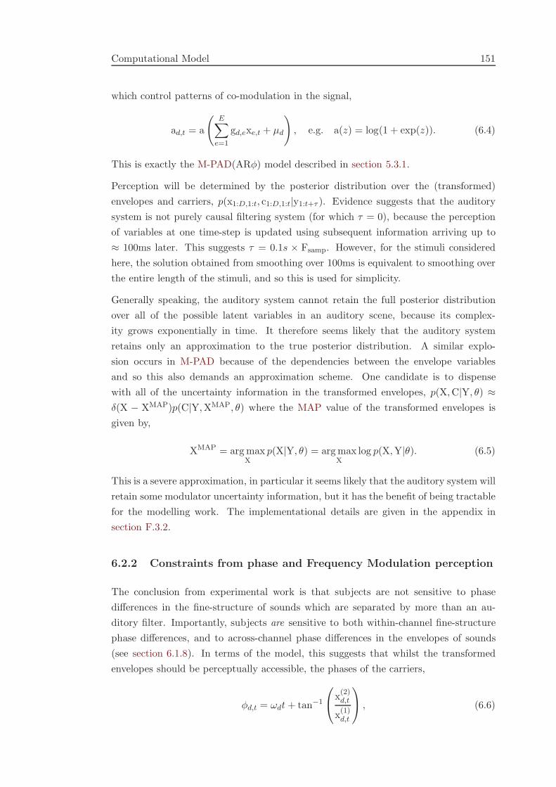
Computational Model 151
which control patterns of co-modulation in the signal,
ad,t = a
(
E∑
e=1
gd,exe,t + µd
)
, e.g. a(z) = log(1 + exp(z)). (6.4)
This is exactly the M-PAD(ARφ) model described in section 5.3.1.
Perception will be determined by the posterior distribution over the (transformed)
envelopes and carriers, p(x1:D,1:t, c1:D,1:t|y1:t+τ ). Evidence suggests that the auditory
system is not purely causal filtering system (for which τ = 0), because the perception
of variables at one time-step is updated using subsequent information arriving up to
≈ 100ms later. This suggests τ = 0.1s × Fsamp. However, for the stimuli considered
here, the solution obtained from smoothing over 100ms is equivalent to smoothing over
the entire length of the stimuli, and so this is used for simplicity.
Generally speaking, the auditory system cannot retain the full posterior distribution
over all of the possible latent variables in an auditory scene, because its complex-
ity grows exponentially in time. It therefore seems likely that the auditory system
retains only an approximation to the true posterior distribution. A similar explo-
sion occurs in M-PAD because of the dependencies between the envelope variables
and so this also demands an approximation scheme. One candidate is to dispense
with all of the uncertainty information in the transformed envelopes, p(X,C|Y, θ) ≈δ(X − XMAP)p(C|Y,XMAP, θ) where the MAP value of the transformed envelopes is
given by,
XMAP = arg maxX
p(X|Y, θ) = arg maxX
log p(X,Y|θ). (6.5)
This is a severe approximation, in particular it seems likely that the auditory system will
retain some modulator uncertainty information, but it has the benefit of being tractable
for the modelling work. The implementational details are given in the appendix in
section F.3.2.
6.2.2 Constraints from phase and Frequency Modulation perception
The conclusion from experimental work is that subjects are not sensitive to phase
differences in the fine-structure of sounds which are separated by more than an au-
ditory filter. Importantly, subjects are sensitive to both within-channel fine-structure
phase differences, and to across-channel phase differences in the envelopes of sounds
(see section 6.1.8). In terms of the model, this suggests that whilst the transformed
envelopes should be perceptually accessible, the phases of the carriers,
φd,t = ωdt+ tan−1
x(2)d,t
x(1)d,t
, (6.6)

Computational Model 152
should not. However, the (possibly smoothed) instantaneous-frequencies, φd,t = φd,t −φd,t−1, must be accessible. This idea is not only consistent with the psychophysical
data, but also with sound coding strategies that transmit the derivatives of the phase
in each sub-band (Flanagan and Golden, 1966).
Another important constraint from experimental work is that auditory processing is
just as sensitive to incoherent frequency modulation in widely separated carriers, as
it is to coherent frequency modulation (see section 6.1.3.2). This is also true in the
model, because the carriers are modelled as independent.
6.2.3 Proximity as inference
The grouping principle of proximity is illustrated in figure 6.1 (see section 6.1.1 for a
review). The first stimulus shown in the figure is an alternating sequence of tones of 80
and 120Hz, that are widely separated. These are heard as separate streams of tones.
In the second stimulus, the gap between the tones has been narrowed and they are
then are heard as a single group. The figure also indicates that a version of M-PAD
can reproduce this effect when it contains a pair of independently modulated carrier
processes,
yt = a1,tc1,t + a2,tc2,t. (6.7)
where the carrier centre frequencies are 80 and 120Hz and the FWHM bandwidths
50Hz. The time-scales of the modulators were set to 200ms. In the figure, the MAP
inferences for a1,t are shown in blue, and a2,t in red. For the first stimulus, the envelope
activity alternates, indicating that the tones remain separate in the model. In the sec-
ond stimulus, the amplitude of the low frequency component remains active throughout,
whilst the high-frequency component remains inactive. This indicates that the tones are
grouped together. The panels below the waveform show the instantaneous frequency
estimates of the model (φ1,t in red, and φ2,t in blue), and ground truth (black). For
the second stimulus, the instantaneous frequency tracks that of the component tones.
Practically, the posterior distribution over the instantaneous frequencies can be esti-
mated using a sampling method called the forward-filter, backward sample algorithm
(see section F.3.4 in the appendices). The figure shows the mean and one-standard
deviation error-bars in the estimates. For clarity, when the envelope of the component
drops below a threshold, it is not plotted.
Importantly, the finding that inference in M-PAD replicates grouping by proximity
is robust against changes to the parameters. The conditions which must be met are
that the carrier processes should be relatively near the tone centre-frequencies, and
the bandwidths wide enough to cover both tones to some degree. The crucial factor is
that the time-scale of the envelopes should be shorter than the gap between the tones
which are not grouped, and longer than the gap between the stimuli that are grouped.

Computational Model 153
Grouping then arises because of a mismatch between the long time-scale in the prior,
and the short time-scale in the signal.
0
sign
al 1
0
100
freq
uenc
y /H
z
0
sign
al 2
0 0.5 1 1.5 2 2.5 3 3.5 4 4.5 5 0
100
time /s
freq
uenc
y /H
z
Figure 6.1: Grouping by proximity as inference. The top two panels show thefirst alternating tone stimulus, and the bottom two show the second. Withineach pair of panels, the top one shows the signal waveforms and the MAP (trans-formed) envelopes, and the bottom one shows the frequency of the tones and theposterior distribution over the instantaneous frequencies of the carriers. For moreinformation, see the text.
In the next section, an identical model is used to explain grouping by good continuation.
6.2.4 Good continuation
The grouping principle of good continuation is illustrated in figure 6.2 (see section 6.1.2
for a review). The first stimulus is an alternating tone sequence (80 and 140Hz) which
separates into two streams as before. In the second stimulus the tones are linked by
smooth frequency-modulated glissandi, and this causes the stimulus to be heard as a
single group. Inference in an identical model to that used in the last section reproduces
this percept. Again, the critical factor is for the envelope process to be slowly varying.

Computational Model 154
0
sign
al 1
0
100
200
freq
uenc
y /H
z
0
sign
al 2
0 0.5 1 1.5 2 2.5 3 3.5 4 4.5 5 0
100
200
time /s
freq
uenc
y /H
z
Figure 6.2: Grouping by good continuation as inference. The top two panels showthe alternating tone stimulus, and the bottom two show the frequency modulatedstimulus. Within each pair of panels, the top one shows the signal waveforms andthe MAP (transformed) envelopes, and the bottom one shows the frequency ofthe tones and the posterior distribution over the instantaneous frequencies of thecarriers. For more information, see the text.
6.2.5 Common Amplitude Modulation
The grouping principle of common amplitude modulation is illustrated in figure 6.3
(see section 6.1.3.1 for a review). In the first half of the stimulus two tones at 80 and
180Hz undergo asynchronous sinusoidal amplitude modulation. In the second half of
the stimulus, the two tones undergo synchronous sinusoidal modulation. Perceptually,
the first half of the stimulus is heard as two independent tones, and the second as a
single, grouped, complex tone.
In order to show that inference can replicate grouping by common AM, it is neces-
sary to extend the model considered in the previous section, because it only contains
independent modulators. The natural extension is to add a third modulator which

Computational Model 155
modulates both of the carriers simultaneously,
yt = (a1,t + a3,t) c1,t + (a2,t + a3,t) c2,t. (6.8)
The envelopes are shown in figure 6.3 (a1,t in red, a2,t in blue, and a3,t in green). In
the first half of the stimulus the independent envelopes are activated asynchronously,
and the third envelope is inactive. However, in the second half of the stimulus, the
situation is reversed indicating that the model groups the two tones.
Once again, this finding is robust to changes in the model parameters. The important
factor is that the prior over the envelopes should be sparse as this introduces com-
petition between the components which then ensures that only one component in the
model is activated in the second half of the stimulus.
0
sign
al
0 0.5 1 1.5 2 2.5 3 3.5 4
100
150
200
time /s
freq
uenc
y /H
z
Figure 6.3: Grouping by common AM as inference. The top panel shows the sig-nal (black) and the envelopes of the three modulators. The lower panel shows thetone frequencies (black lines) and the posterior distribution over the instantaneousfrequencies of the carriers. For more details, see the text.
6.2.6 Closure and the continuity illusion
If a short section of a tone is removed and replaced with noise, sufficient in energy to
have masked the tone were it present, then the tone is heard to continue through the
noise (see section 6.1.6 for a discussion). Similarly, a tone ending in a noise burst is
heard to persist into the noise. Finally, a tone starting after a noise burst, is heard to
begin in the noise. Figure 6.4 illustrates these three examples of the continuity illusion
for a 100Hz tone and a white noise masker of variance 10.
From the perspective of inference, these stimuli are reminiscent of denoising tasks in
which prior knowledge is used to fill-in data in a noisy region. The twist is that the noisy

Computational Model 156
regions have to be inferred from the data, rather than being known a priori. A suitable
model therefore should contain two components, yt = ytonet + ynoise
t . First, a fairly
narrow-band carrier, with a slow modulator, is used to model the tone ytonet = a1,tc1,t.
The experiments use a carrier with a centre-frequency of 100Hz and a bandwidth of
30Hz, and a modulator with a time-scale of 50ms. Second, a broad-band component
with a relatively quickly varying (15ms) modulator is used to model the noise bursts.
One way of modelling the broad-band component is to use a single broad-band carrier,
another is to use a number of co-modulated narrow-band carriers,
ynoiset = a2,t (c2,t + c3,t + c4,t) . (6.9)
This version of the model connects to the experiments on CMR in the next section
and so results are shown in this configuration with centre-frequencies of 70, 100 and
130Hz, and bandwidths of 30Hz. The top panel of figure 6.4 shows the inferences for the
envelopes (a1,t in red and a2,t in blue). The inferences for the instantaneous frequency
of the carrier process c1,t are shown in the panel below. The third panel shows the
inference for the tone component of the model, ytonet (black) and the uncertainty in this
component (grey). In the noisy regions, the mean of the component quickly decays to
zero, but the uncertainty rises. Furthermore, the envelope, a1,t (shown in red), decays
slowly, according to the prior. The bottom panel shows ynoiset in black, together the
envelope a2,t in blue. The conclusion is that the model identifies the noisy regions and
interpolates the envelope of the tone through them. The next section illustrates CMR
which can also be viewed as a denoising task in which the local SNR must be estimated
from the data.
6.2.7 CMR
When a tone is masked by noise of a bandwidth greater than that of an auditory filter,
the tone can become audible if the noise is amplitude modulated (see section 6.1.7 for
a review). This effect, called CMR, is illustrated in figure 6.5 for a 100Hz tone in noise
of variance 2, centred on 100Hz with a cosine shaped spectrum of bandwidth 50Hz.
An identical model to that used in the last section can be used to model CMR. This
model contains a tone component, ytone, with a carrier that has a bandwidth equal
to that of an auditory filter and a slowly varying modulator. The second component
models the noise, ynoise, and contains a more quickly varying modulator and three (or
more) comodulated carriers which are essentially adjacent auditory filters with similar
bandwidths (30Hz) and differing centre frequencies (70, 100 and 130Hz).
Figure 6.5 shows that, in the first condition, the noise component is activated through-
out the stimulus, whilst the tone component remains inactive. In the second condition
the tone is revealed in the dips of the modulator. This activates the tone component,
and the slowness prior interpolates through subsequent peaks in the modulation so that

Computational Model 157
−5
0
5
sign
al
0
50
100
150
freq
uenc
y /H
z
−1
−0.5
0
0.5
1
ytone
0 0.5 1 1.5
−5
0
5
ynois
e
time /s
Figure 6.4: The continuity illusion as inference. The top panel shows the signal(black), and the inferred envelopes of the tone modulator (red) and the noisemodulator (blue). The second panel down shows the posterior distribution overthe instantaneous frequency of the tone carrier. The lower two panels show theinferences for the tone and the noise component respectively (black) and theirassociated envelopes. The uncertainty in the tone component is shown in lightgrey. For more details, see the text.
the component is active throughout the stimulus. The second row of the figure shows
the mean of the noise component of the model (black) and the associated modulator
(blue). The third row shows the mean of the tone component (black) and modulator
(red). The uncertainty in the tone component is shown in grey. The final row shows
the uncertainty in the instantaneous frequency of the tone component in regions where
the amplitude of the tone component is larger than a threshold value of 0.1. The am-
plitude during the first stimulus never crosses this threshold indicating that the tone
is masked. In the second stimulus, the amplitude remains above the threshold for the
duration of the tone indicating that the tone has been released from the masker. This
result requires that the model is sparse because this ensures just a single component is
active for the first stimulus.

Computational Model 158
−4
−2
0
2
4signal 1
−4
−2
0
2
4
ynois
e
−2
0
2
ytone
0 0.5 1 1.5 2 2.580
100
120
freq
uenc
y /H
z
time /s
signal 2
0 0.5 1 1.5 2 2.5
time /s
Figure 6.5: Comodulation masking release as inference. The left hand columnof panels shows the unmodulated condition where the noise masks the tone. Theright hand column of panels shows the modulated condition where the tone isaudible. The top row of panels shows the two signals, and the MAP inferencesfor the two modulators. The second row shows the noise component of the model,and the third row shows the tone component. The bottom row shows the posteriordistribution over the instantaneous frequency of the tone component. For moredetails, see the text.
6.2.8 Old plus new heuristic
An example of the old plus new heuristic is shown in figure 6.6 (see section 6.1.4 for
a review). The stimulus, shown in the top panel, contains four elements separated by
short gaps. The spectral content of the elements is shown in the second panel down.
The first element is a harmonic stack with components at 80, 160 and 240Hz. The
second element is also a harmonic stack with components at 160 and 320Hz. These
elements are perceived veridically and are provided for comparison with the last two
elements. The third element contains a pure 160Hz sinusoid to which a harmonic stack
is added at the mid-point with components at 80 and 240Hz. Importantly, the tone is
perceived to be constant for the duration of the element, and therefore separate from
the two component stack. The fact that the second half of the element is essentially

Conclusions and future directions 159
identical to the first element in the stimulus, but it is not perceived as such, shows
that context is important in grouping. The final element of the stimulus begins with
a harmonic stack with components at 160 and 320Hz. At the mid-point the stimulus
switches to a three component harmonic stack with harmonics at 80, 160 and 240Hz.
This element is identical to the third, except for the addition of a 320Hz tone to the first
half. However, this small change is important because it is grouped with the 160Hz
tone, and this prevents the tone from capturing the 160Hz harmonic of the second
stack. Instead, the element is perceived as a two harmonic stack, followed by a three
harmonic stack.
One way of modelling this stimulus is to use four carriers with centre frequencies near to
the four tones that appear in the signal and bandwidths equal to that of corresponding
auditory filters. These carriers are modulated in four different patterns,
yt = a1,t
3∑
k=1
ck,t + a2,t (c2,t + c4,t) + a3,tc2,t + a4,t (c1,t + c3,t) . (6.10)
The first pattern involves the three lowest frequency carriers (80, 160 and 240Hz), the
second pattern involves two carriers (160 and 320Hz), third pattern is a pure tone
(160Hz) and the fourth pattern again involves two components (80 and 240Hz). The
time-scales of these modulators are equal and set to 200ms. All of the prior activations
of the components are sparse, so there is competition between them. The results of
inference are shown in figure 6.6. Importantly, in the third element the tone component
(a3,tc2,t) is inferred as continuing throughout the subsequent harmonic stack. This effect
arises because of the slow prior on the envelope variable.
6.3 Conclusions and future directions
This chapter has argued that auditory perception is inference. As a first test of this
hypothesis, we have demonstrated that inference in a model for primitive auditory
scene statistics qualitatively replicates the primitive grouping rules that listeners use
to understand simple acoustic scenes. The model comprises a sum of comodulated
coloured noise carriers. Inference for these modulators and carriers can replicate the
grouping principles of proximity, good continuation, common-fate as well as the con-
tinuity illusion, comodulation masking release, and the old plus new heuristic. This
paves the way for a full analysis in which a model trained on natural sounds is tested
with experimental stimuli in order to determine whether it quantitatively matches psy-
chophysical data. This raises the tantalising possibility of predicting the results of new
psychophysical experiments purely from the statistics of natural sounds.
In order to capture the full range of psychophysical phenomena it is likely that im-
provements will have to be made to the model and the inference scheme, and also to

Conclusions and future directions 160
−2
0
2
0
200
400
freq
uenc
y /H
z
−202
a 1
−202
a 2
−101
a 3
0 0.5 1 1.5 2 2.5 3 3.5 4−2
02
a 4
time /s
Figure 6.6: The old plus new heuristic as inference. The top panel shows thesignal and the MAP inferences for the four modulators in the model. The secondpanel down shows the true frequencies of the tones present in the signal, and theposterior distribution over the instantaneous frequencies of the carriers, colouredby the modulator which is activating them. The final four panels show the fourcomponents in the model with associated modulators and the contribution theymake to the signal (black). For more information, see the text.
incorporate online learning.
With regard to improvements in the model, one obvious direction is to model binaural
data. Another extension is motivated by the observation that CMR is sensitive to
multiple time-scales in the modulation (see section 6.1.7). This suggests that the model
should be extended to contain a hierarchy of modulators of different time-scales. We
have already argued for an extension of this sort in Chapter 4, based on the statistics
of natural scenes (see section 5.4). The idea was to combine two sets of modulators via
a product and mix them via a set of positive weights,
ad,t =∑
l,m
Wd,l,ma(1)l,t a
(2)m,t. (6.11)
Modulators in higher levels of the hierarchy would tend to be slower than lower level

Conclusions and future directions 161
modulators, capturing statistical structure like sentences, rather than phonemes. In
fact, grouping at the level of this second layer of modulators would appear to provide a
more satisfactory match to the proximity principle; the carriers capture the frequency
content of the tones, the first layer of modulators capture the envelopes of the individual
tones, and the second layer of modulators capture the presence of the entire stream
of tones. This division accords more closely to perception, and the time-scales are a
better match to experimental data. More general, hierarchical extensions of the model
potentially provide a way of combining primitive and schema-based grouping into a
single computational framework.
With regard to improvements in the inference scheme, one example where the current
scheme is not sufficient to explain perception is the perceptual bistability that arises
for intermediate settings of the alternating tone stimulus. This could potentially be
explained if the posterior distribution was itself bimodal and if perception was switching
between these modes. However, this suggests a non-point like inference scheme is
necessary for modelling work, like a sampling method.
With regard to online-learning, one observation which bears the hallmarks of online-
learning is the fact that in the alternating tone task subjects tend to be more likely to
perceive the two stream percept as time passes.

Chapter 7
Conclusion
The purpose of this thesis was to develop statistical models for natural sounds. The
new statistical models were developed using traditional signal processing methods as
a starting point. Next a probabilistic model was identified in which inference approxi-
mated the original deterministic procedure. Finally, the new probabilistic method was
compared and contrasted to the original deterministic approach. The new algorithms
often performed better, as well as being more flexible, but the cost is a much larger
computational demand and longer processing times. This general idea, of probabilising
traditional signal processing methods, was one of three major themes of the thesis.
Traditional signal processing representations are useful because they reveal the im-
portant statistics of natural signals. For example, short sections of sounds are often
composed of a relatively small number of sinusoidal components and so time-frequency
analysis is popular tool. This link between useful representations of sounds and their
statistics means that it is important to characterise the statistics of natural sounds.
Fortunately, the new probabilistic methods can be used to unpack these statistics by
determining what aspects of sounds they fail to capture. This endeavour was the second
main theme of the thesis.
It is likely that auditory processing is matched to the statistics of natural sounds. For
example, the first stage of auditory processing is a time-frequency analysis with proper-
ties that are well matched to the spectral-temporal statistics of sounds. Furthermore, it
appears that perception is often based on the long-time statistics of sounds rather than
on the raw waveform. One unifying perspective, with a long history, that accounts for
these observations is that hearing is inference. The connection between the statistics
of sounds and inference is the third theme of this thesis.
As the thesis contains three different, but related themes, the conclusions have been
broken down thematically.

Probabilising signal processing methods 163
7.1 Probabilising signal processing methods
Many signal processing problems are ill posed because they involve estimating two
or more variables at each time-step from a one dimensional signal. This observation
motivates a new perspective, which is to view them as inference problems and to de-
rive alternative representations using the calculus of inference; Bayesian probability.
This thesis applies this approach to a range of signal processing problems including
demodulation, time-frequency analysis, and sub-band demodulation. Generally speak-
ing, the new probabilistic methods are considerably slower than their deterministic
counterparts, but they have several significant advantages.
The first technique to be probabilised in this way was amplitude demodulation. Al-
though there are many existing methods for estimating the envelopes of signals, there
are well documented problems with all of these approaches (see chapter 2). Never-
theless, in spite of these deficiencies, demodulation methods are used extensively in a
range of applications including; audio compression, audio manipulation, audio retrieval,
speech and music recognition, and in cochlear implants. This indicates that the modu-
lation content of sounds is a defining characteristic and that it is important to estimate
it accurately. We introduced the probabilistic approach to demodulation called Prob-
abilistic Amplitude Demodulation (PAD) in chapter 3, providing a family of methods
for inferring the envelope of a signal. PAD was validated in a number of ways. Firstly,
it was applied to synthetic signals where ground truth was known, and it was shown
to be more accurate than traditional approaches. It is hard to evaluate demodulation
methods on natural signals quantitatively, but qualitatively, the solutions from PAD
often appear superior. They also have several desirable properties, like the fact that
demodulating a carrier recovered from PAD yields a constant envelope. This important
consistency test indicates that the signal has been demodulated, and traditional ap-
proaches fail it catastrophically. Not only does PAD provide higher quality estimates of
the carrier and modulator, the approach also offers several other advantages over tra-
ditional methods. For instance, because uncertainty is handled automatically, the new
method is more robust to noise, it can fill in envelopes in missing regions of the signal,
and it can return error-bars that indicate the uncertainty in the estimates. Further-
more, the parameters of the model, like the time-scale of the envelope, the modulation
depth, and the frequency content of the carriers, can be learned from the signal. This
automates the methods and avoids the need for heuristic hand-tuning of parameters
which often complicates the application of other methods. Perhaps the greatest advan-
tage of the probabilistic approach is that it is relatively simple to extend and combine
models. For example, PAD can be extended to model signals with multiple time-scales
of modulation using a representation called a demodulation cascade (see chapter 4).
The number of levels in the cascade, and the time-scales of each level can be learned
from data.
The second set of methods that were probabilised were those of time-frequency analy-

Unpacking the statistics of natural sounds 164
sis. We provided probabilistic versions of filter banks, the STFT and the spectrogram.
These models were based on linear Gaussian State Space models and so the represen-
tations can be derived by Kalman Smoothing. The new methods are complementary
to traditional approaches because, whilst inference is relatively slow, resynthesis is fast,
simple and principled. We provide methods for learning the parameters of the proba-
bilistic time-frequency representations, like the filter properties. The main purpose for
developing these models was to combine them with models for modulation in order to
produce more powerful representations. This led to the third set of new probabilistic
methods called Multivariate Probabilistic Amplitude Demodulation (M-PAD), which
describe sounds in terms of a sum of amplitude co-modulated narrow-band carriers.
Versions of M-PAD can perform probabilistic sub-band demodulation and others are
probabilistic versions of the MQ algorithm and harmonic plus noise analysis. One
major advantage of the probabilistic approach is that it reduces the number of free-
parameters and it provides methods for learning the remainder from data. The utility
of the new methods were demonstrated on a missing data task in which M-PAD was
used to accurately reconstruct in missing sections of speech up to 20ms long.
7.2 Unpacking the statistics of natural sounds
Sounds are known to have extremely rich statistical structure. For example, model free
studies have shown that sounds are very sparse and that spectral-temporally they are
sparser still. Moreover, the Hilbert Envelope (HE) of the filter coefficients is known to
exhibit long-time dependencies (up to 100ms long) and wide cross-frequency dependen-
cies (over thousands of Hz). However, prior to this work, probabilistic models which
capture these important properties of natural sounds have not been developed.
In chapter 3 we focussed on the modulation content of sounds and built a family of
models called PAD that accounted for some of these statistics. By applying PAD to
sound waveforms and sound filter coefficients many of the established results concerning
the statistics of natural sounds were confirmed. In particular, we showed that natural
sounds exhibit strong modulation (average statistical modulation depths of 0.9) over
a wide range of time-scales (1ms-390ms) and across widely separated sub-bands. In
addition, we found that the sub-band statistics of modulation appeared to be sufficient
to distinguish different sound classes, like animal vocalisations, transients, auditory
textures, and complex acoustic scenes. Moreover, we showed that natural sounds often
contained specific patterns of co-modulation.
In order to investigate this further, chapter 5 generalised PAD so that it comprised
multiple carriers that underwent patterns of comodulation. The new model, called
M-PAD, was a temporal version of GSMs, which have been a popular tool for studying
natural scene statistics. M-PAD was applied to a variety of natural sounds in order to
learn the patterns of modulation, their time-scales, and the properties of the carriers

Probabilistic Auditory Scene Analysis 165
in the sound. The conclusion was that the power, sparsity (or the modulation depth),
and skew in each sub-band of the signal, together with the patterns of modulation and
their time-scale, were sufficient to produce realistic sounding auditory textures. This
indicates that simple auditory textures are largely defined by these statistics. However,
it was not possible to generate realistic versions of more complex sounds, like animal
vocalisations, indicating that they contain other important statistical structure, like
asymmetric pulse-resonances and frequency sweeps.
It is hoped that the ability to generate controlled, but natural sounding acoustic tex-
tures from a generative model will be of use to experimentalists. These stimuli fall
in an important empty middle ground between tones and noise (which are simple to
control, but sound unnatural) and natural sounds (which are uncontrolled).
7.3 Probabilistic Auditory Scene Analysis
One of the claims of this thesis is that perception often operates at the level of the
statistics of sounds, rather than at the level of the raw waveform. For example, when
artificial sounds are generated with statistics that match those of natural auditory
textures, they are perceived as coming from the same type of source as the original,
even though the raw waveforms are quite different (see chapter 5). This observation
is unsurprising because, for example, no two natural rain sounds will be precisely the
same, but they are still perceived as arising from the same type of source. Nevertheless,
it does beg an important question: What type of statistics is the auditory system
sensitive too?
We have previously argued that AM appears to be an important statistical regularity
in natural sounds and this implies that the auditory system should listen attentatively
to its statistics, which include the time-scales, modulation-depth and cross-frequency
patterns of co-modulation. There is a great deal of evidence from psychophysics which
indicates that this is the case. For instance, AM is a strong cross-frequency grouping
cue and it has been implicated in a large number of psychophysical tasks on many
different time-scales. However, although there is a wealth of evidence that AM is
important behaviourally, it is not completely clear how that is reflected in the neural
organisation. One of the consequences of the paucity of concrete experimental data on
the neural processing of AM is that the modelling work in this thesis focuses on the
psychophysics data.
The main theoretical idea explored in this theme of the thesis is that hearing is inference.
This perspective is an old one, but it is compatible with the idea that perception is
often based on the statistics of sounds and that auditory processing is optimised with
respect to these statistics. More specifically, we introduced a model for primitive natural
sound statistics and demonstrated that many psychophysical phenomena in primitive

Probabilistic Auditory Scene Analysis 166
auditory scene analysis were consistent with inference in this model. The model, a
version of M-PAD, contained coloured noise carriers that underwent patterns of co-
modulation. Inference for the modulators and the carriers reproduced the grouping
principles of proximity, good continuation and common fate, as well as the continuity
illusion, comodulation masking release, and the old plus new heuristic. This qualitative
analysis paves the way for a quantitative version where the model is trained on a corpus
of natural sounds, then tested on psychophysical stimuli, and finally compared to the
data from listeners. This raises the tantalising possibility of predicting the results of
new psychophysical experiments directly from the statistics of natural scenes.

Appendix A
Circulant Matrices
This appendix briefly surveys relevant material on circulant matrices and their rela-
tionship to stationary covariance matrices. This leads to efficient methods for learning
and inference using stationary GPs over regularly sampled points (see chapter 2). For
more details on circulant matrices see Davis (1979).
A.1 Circulant Matrices
A T by T matrix C is circulant if each column is a shifted version of the others,
C =
c0 cT−1 cT−2 . . . c2 c1
c1 c0 cT−1 . . . c3 c2
c2 c1 c0 . . . c4 c3...
......
. . ....
...
cT−2 cT−3 cT−4 . . . c0 cT−1
cT−1 cT−2 cT−3 . . . c1 c0
. (A.1)
The above can be written in index notation as Ct,t′ = cmod(t−t′,T ). The eigenvectors of
circulant matrices are complex exponentials. This can be shown as follows,
gt′ =T−1∑
t=0
Ct′,t exp(−2πikt/T ) =T−1∑
t=0
cmod(t′−t,T ) exp(−2πikt/T ) (A.2)
=
T−1−t′∑
u=−t′
cmod(u,T ) exp(−2πik(t′ + u)/T ) (A.3)
= exp(−2πikt′/T )T−1−t′∑
u=−t′
cmod(u,T ) exp(−2πiku/T ) (A.4)
= exp(−2πikt′/T )λt′,k (A.5)

Circulant Matrices 168
To complete the proof it is necessary to show that λt′,k is independent of t′,
λt′,k =
T−1−t′∑
u=−t′
cmod(u,T ) exp(−2πiku/T ),
=
c0 + c1 exp(−2πik/T ) + · · · + cT−1 exp(−2πi(T − 1)k/T )
cT−1 exp(2πik) + c0 + · · · + cT−2 exp(−2πi(T − 2)k/T )...
c1 exp(2πik(T − 1)/T )c0 + c2 exp(2πik(T − 2)/T ) + · · · + c0
,
=
T−1∑
t=0
ct exp(−2πikt/T ) = ck. (A.6)
Therefore, the eigenvalues of C are the Fourier transform of the row vector cu. The
eigen-decomposition of circulant matrices (Ct,t′ = 1T
∑
k exp(2πik(t− t′)/T )ck) leads to
fast methods for computing with them because the FFT can be used. For example, the
multiplication g = Cx, can be computed efficiently using
gt =∑
t′
Ct−t′xt′ =1
T
∑
t′,k
exp(2πik(t − t′)/T )ckxt′ , (A.7)
=1
T
∑
k
exp(2πikt/T )xk ck =∑
k
FT−1t,k xkck. (A.8)
Matrix multiplication is therefore equivalent to point-wise multiplication of the two
DFTs, followed by an inverse Fourier transform of the result. Similarly, the quadratic
form g = xTCx, can be computed quickly by,
g =1
T
∑
k,t
exp(2πikt/T )xtxkck =1
T
∑
k
x∗kxk ck =1
T
∑
k
|xk|2ck. (A.9)
Quantities involving the inverse of a circulant matrix can be handled in a similar man-
ner. Consider, h = C−1x which implies that, x = Ch. Using the above results, this
means xk = hk ck. Rearraging and using the inverse DFT gives,
ht =1
T
∑
k
exp(2πikt/T )xk
ck=∑
k
FT−1t,k
xk
ck. (A.10)
Thus matrix multiplication by a matrix inverse is equivalent to the point-wise division
of the two DFTs followed by an inverse Fourier transform. For completeness, the
quadratic form, h = xTC−1x, is given by
h =1
T
∑
k
|xk|2ck
. (A.11)
Finally, the determinant of a circulant matrix is also easy to compute using the fact
that a determinant is a product of the absolute values of a matrix’s eigenvalues and

Stationary Covariance Matrices on regularly sampled points 169
this, for ciculant matrices, is the product of the absolute value of the Fourier transform
coefficients,
det(C) =∏
k
|ck|. (A.12)
A.2 Stationary Covariance Matrices on regularly sampled
points
Stationary covariance matrices on T regularly sampled points take the following form
S =
s0 s1 s2 . . . sT−2 sT−1
s1 s0 s1 . . . sT−3 sT−2
s2 s1 s0 . . . sT−4 sT−3
......
.... . .
......
sT−2 sT−3 sT−4 . . . s0 s1
sT−1 sT−2 sT−3 . . . s1 s0
. (A.13)
Covariance matrices of this form are therefore not circulant. However they can embed-
ded into a larger 2(T − 1) × 2(T − 1) circulant matrix,
S′ =
s0 s1 . . . sT−2 sT−1 sT−2 sT−3 . . . s2 s1
s1 s0 . . . sT−3 sT−2 sT−1 sT−2 . . . s3 s2...
.... . .
......
......
. . ....
...
sT−2 sT−3 . . . s0 s1 s2 s3 . . . sT−2 sT−1
sT−1 sT−2 . . . s1 s0 s1 s2 . . . sT−3 sT−2
sT−2 sT−1 . . . s2 s1 s0 s1 . . . sT−4 sT−3
sT−3 sT−2 . . . s3 s2 s1 s0 . . . sT−3 sT−2
......
. . ....
......
.... . .
......
s2 s3 . . . sT−2 sT−3 sT−4 sT−3 . . . s0 s1
s1 s2 . . . sT−1 sT−2 sT−3 sT−2 . . . s1 s0
=
[
S P
P T Q
]
. (A.14)
Multiplication, f = Sx can then be handled using the following,
[
f
g
]
=
[
S P
P T Q
][
x
0
]
= Sx, (A.15)
which can be computed quickly using FFTs as described in the last section. Unfortu-
nately there are no tricks for computing expressions involving the inverse of S in terms

Stationary Covariance Matrices on regularly sampled points 170
of the FFT of the circulant matrix, S. This is why chapter 3 introduces the approach
of augmenting observed data with missing data in order to make the covariance matrix
circulant (see section 3.2.2).
Finally, we note that for a stationary covariance with a typical time-scale of variability
τ , in the limit of observing a large number of time-scales (T/τ → ∞),
S−1x→ 1
T
∑
k
FT−1t,kxksk. (A.16)

Appendix B
Weight space view of stationary
Gaussian Processes
This section provides an alternative view of the stationary Gaussian process prior which
connects the formalism of chapter 3 with that of Bretthorst (1988). For more informa-
tion about Gaussian Processes, see Rasmussen and Williams (2006).
In this section we will construct a prior over a real signal xt in two stages. In the first
stage we draw a set of complex valued weights wk according to a Gaussian distribution
and in the second we generate the signal by using theses weights to linearly combine
a set of basis functions bk. If the signal is stationary, one suitable choice for the basis
functions are complex exponentials. In other words the signal is given by the DFT of
the weights,
xt =
T∑
k=1
wkbk =
T∑
k=1
wk1√T
exp(−2πi(k − 1)(t − 1)/T ). (B.1)
The factor 1√T
ensures the basis functions are normalised. In order to make the no-
tation simple to understand, we will assume that T , the length of the data, is even.
Furthermore, it is useful to symmetrise this expression for the signal so that,
xt =
T/2∑
k=−T/2
wkbk =1√T
T/2∑
k=−T/2
wk exp(−2πikt/T ). (B.2)
The weights are complex valued and so, in order for the signal to be real, they have to be
constrained so they are complex-conjugate symmetric, wk = w∗−k. The real and imagi-
nary components of the weights wk = uk + ivk, will be drawn independently from zero
mean Gaussians of the same variance, p(uk) = p(vk) where p(uk) = Norm(uk; 0,12s
2k).
In other words, each weight can be thought of as a two dimensional vector drawn from
an isotropic Gaussian. The mysterious factor of one half comes from the fact that we
will be interested in the average square magnitude of the weights which then takes a

172
simple form 〈|wk|2〉 = s2k. Notice also that the average square of the weights is zero,
〈w2k〉 = 〈a2
k〉−〈b2k〉+2i〈akbk〉 = s2k−s2k = 0. Importantly, by construction, the frequency
content of xt is uncorrelated. That is, 〈wkwk′〉 is zero when k 6= k′.
The Gaussian distribution over the weights induces a Gaussian distribution over the
data (as the Gaussian family is closed under linear transformations). The moments of
the resulting Gaussian are found as follows. First the mean,
〈xt〉 =1√T
T/2∑
k=−T/2
〈wk〉 exp(−2πi(k − 1)(t− 1)/T ) = 0. (B.3)
The variance is a little more complicated, but using the fact that the signal is real,
xt = x∗t , we have,
〈xtxt′〉 =1
T
T/2∑
k=−T/2
T/2∑
k′=T/2
〈wkw∗k′〉 exp(−2πikt/T ) exp(2πikt′/T ) (B.4)
the key quantity is the covariance of the weights, 〈wkw∗k′〉 = δk,k′〈|wk|2〉+ δk,−k′〈w2
k〉 =
δk,k′s2k, and this means that the covariance of the data is,
〈xtxt′〉 =1
T
T/2∑
k=−T/2
s2k exp(−2πik(t− t′)/T ) =
T/2∑
k,k′=−T/2
FTt,ks2kδk,k′FT−1
k′,t′ . (B.5)
The inverse covariance of the Gaussian distribution over the signal is therefore (see
appendix A),
Σ−1 =
T/2∑
k,k′=−T/2
FTt,k1
s2kδk,k′FT−1
k′,t′ . (B.6)
This means the Gaussian distribution over the signal can be written,
p(x1:T |s21:K) =
T/2∏
k=−T/2
(2πs2k)−1/2 exp
(
− 1
2Ts2k|xk|2
)
, (B.7)
This is a Gaussian process prior (e.g. equation (3.39)) when s2k = γk. This makes
explicit the relationship between Bretthorst (1988) and this work. The former operates
in weight space, and describes models in terms of (a usually small number of) weighted
sinusoids. The latter operates in function space, and describes models using the induced
Gaussian process prior over the signal. For a more general discussion of the weight-
space and function-space view of GPs, see Rasmussen and Williams (2006).

Appendix C
Auto-regressive processes
This appendix briefly reviews the theory of AR processes relevant to this thesis. For
an introduction to AR processes, see Chatfield (2003).
C.1 Preliminaries
A τ th order Gaussian auto-regressive process (denoted AR(τ)) is given by,
xt =τ∑
t′=1
λt′xt−t′ + ǫtσ, ǫt = Norm(ǫt; 0, 1). (C.1)
For example, if τ = 2 then xt = λ1xt−1 + λ2xt−2 + ǫtσ. This means that the current
value of the process is given a weight sum of the previous τ = 2 values (hence the name
auto-regressive), plus some Gaussian noise (of variance σ2). Typical samples from an
AR(2) process can be seen in Figure C.1.
0 5 10 15 20 25 30 35 40 45 50−3
−2
−1
0
1
2
time /samples
x t
Figure C.1: Three samples from the stationary distributio of an AR(2) processwhere λ = [1.5697,−0.7787]T and σ2 = 1/10.

Stationarity 174
In this note several important properties of these processes are computed. For example,
certain choices of λ results in a non-stationary process that blows up to infinity (e.g. τ =
1 and λ > 1), but for other choices the process is stationary. It is therefore useful to
have an expression which determines whether the process is stationary. This is the
subject of section C.2.
AR(τ) processes are a parameterisation of a Gaussian distribution over x1:T . Gaussian
random variables are completely described by their mean and covariances. The mean
of a stationary auto-regressive process is zero. However, the covariance, which is also
called the auto-correlation, is more complicated. In section C.3 an expression is given
for the auto-correlation.
Stationary processes have covariance matrices which have sinusoidal eigenvectors. The
eigenvalues therefore completely determine stationary processes and these are called
the power-spectrum of the process. This quantity will also be derived in this note
in section C.4. The power-spectrum and the auto-correlation are intimately related,
formally one can switch between them using the Fourier transform. The mean of the
spectrum is the marginal variance.
Sections C.3 and C.4 of this note describe how to move from the parameters of the
AR(τ) process to the auto-correlation and power-spectrum, which are essentially prop-
erties of the Gaussian process over x1:T . To flip this on its head, we are often interested
in moving in the opposite direction. That is, to derive the parameters of an AR(τ) pro-
cess from an auto-correlation or power-spectrum. For example, we may need to specify
an AR(τ) prior for some quantity for which we know the power-spectrum. Methods for
doing that are developed in section C.5.
C.2 Stationarity
A one dimensional AR(τ) process can be written as a τ dimensional AR(1) process by
defining a new state-space xt = [xt, xt−1, . . . , xt−τ+1]T, so that xt = Λxt−1 + σǫt, where
the new dynamics matrix is given by,
Λ =
λ1, λ2, . . . λτ−1, λτ
1, 0, . . . 0, 0
0, 1, . . . 0, 0...
.... . .
......
0, 0, . . . 1, 0
, (C.2)

Stationarity 175
−2 −1.5 −1 −0.5 0 0.5 1 1.5 2
−1
−0.5
0
0.5
1
λ1
λ 2
Figure C.2: The triangular region of the λ1-λ2 plane which corresponds to sta-tionary AR(2) processes is shown by the black dots (λ2 < 1 − λ1, λ2 < 1 + λ1
and λ2 > −1). The red dot indicates the process with λ = [1.5697,−0.7787]T isstationary.
and the new noise by,
ǫt = Norm
ǫt;
0
0...
0
,
1, 0, . . . 0
0, 0, . . . 0...
.... . .
...
0, 0, . . . 0
. (C.3)
This relationship is useful computationally. Importantly, it also leads to a set of analytic
conditions which must be met for an AR(τ) process to be stationary. These conditions
are found by noticing that the process will be stationary if the eigenvalues of Λ are less
than or equal to unity (α ≤ 1). The simple form of Λ means there is a correspondingly
simple expression for the eigenvalues,
ατ =
τ∑
t=1
λtατ−t. (C.4)
So, for an AR(2) process, the above expression is a quadratic in α, the solutions of
which are given by, α = 12λ1 ±
√
14λ
21 + λ2. Using this result, the domain of stationary
processes is plotted in Figure C.2.

Auto-correlation 176
C.3 Auto-correlation
The auto-correlation can be derived by solving a set of τ independent linear equations
for 〈xtxt+t′′〉. Suitable equations are found by taking the residuals,
ǫt = xt −τ∑
t′=1
λt′xt−t′ , (C.5)
and finding their auto-correlation, 〈(xt −∑τ
t′=1 λxt−t′) (xt+a −∑τt′=1 λxt−t′+a)〉τ−1
a=0.
Simplfying, this becomes,
〈ǫtǫt+a〉 = σ2δa,0 =〈xtxt+a〉 −τ∑
t′=1
λt′〈xt−t′xt+a〉 −τ∑
t′=1
λt′〈xtxt+a−t′〉
+τ∑
t′=1
τ∑
t′′=1
λt′λt′′〈xt−t′xt+a−t′′〉 (C.6)
This is a system of linear equations involving the elements of the auto-correlation
function and can be written, ai =∑τ−1
j=0 Bi,j〈xtxt+j〉, where a = [σ2, 0, . . . , 0]T and
B =
1 +∑τ
t=1 λ2t , 2
∑τ−1t=1 λtλt+1 − λ1, . . . λ1λτ − λτ−1, −λτ
λ1, λ2 − 1, . . . λτ , 0
λ2, λ1 + λ3, . . . 0, 0...
.... . .
......
λτ−1, λτ−2 + λτ , . . . −1, 0
λτ , λτ−1, . . . λ1, −1
. (C.7)
This can be solved using matrix inversion to give the auto-correlation. For example,
if τ = 2 then the marginal variance is, 〈x2t 〉 = (1−λ2)σ2
1−λ21−λ2
2−λ2−λ21λ2+λ3
2. The complete
autocorrelation function is shown in Figure C.3). In the next section we find an analytic
expression for the power spectrum. A computationally less expensive proceedure to find
the auto-correlation is to find the inverse FFT the power-spectrum.
C.4 Power Spectrum
Unlike the auto-correlation function, the power-spectrum has a closed form solution.
One method for deriving the power-spectum of a process, is to form the auto-correlation
function γ(τ) = 〈xtxt+τ 〉, and then Fourier transform this quantity. Perhaps the easiest
method is to consider the auto-correlation of the residuals, which was used in the
last section (Equation (C.6)), and then to find the discrete Fourier Transform of this
quantity, defined as FT (f(t)) =∑T−1
t=0 f(t) exp(iωt). The shift-propery of the discrete
FT simplifies much of the work, FT (f(t+ δ)) = exp(iωδ)f(ω), using this relationship,

Power Spectrum 177
0 5 10 15 20 25 30 35 40−0.5
0
0.5
1
1.5
time lag
auto
−co
rrel
atio
n
Figure C.3: The autocorrelation of an AR(2) process. λ = [1.5697,−0.7787]T
and σ2 = 1/10.
we have
σ2∑
τ
exp(iωτ)δτ,0 = σ2 =γ(ω)
(
1 −τ∑
t=1
λt exp(iωt) −τ∑
t=1
λt exp(−iωt)
+
τ∑
t=1
τ∑
t′=1
λtλt′ exp(iω(t− t′))
)
(C.8)
which can be rearranged to give the power-spectrum
γ(ω) =σ2
1 +∑τ
t=1 λ2t − 2
∑τt=1 λt cos(ωt) + 2
∑τt=1
∑τt′=t+1 λtλt′ cos(ω(t− t′))
(C.9)
So, for example, the spectrum of a typical AR(2) process is given by,
γ(ω) =σ2
(1 + λ21 + λ2
2) + 2λ1(λ2 − 1) cos(ω) − 2λ2 cos(2ω). (C.10)
An example of which is shown in Figure C.4. Other useful expressions include the
frequency at the maximimum of the spectrum as well as the bandwidth (defined by the
Full Width Half Maximum) of the spectrum,
cosωMAX =λ1
4λ2(λ2 − 1) (C.11)
cosωFWHM = cosωMAX ± 1
4
√
−8 − 41 + λ2
1 + λ22
λ2− λ2
1
λ22
(λ2 − 1)2 (C.12)
Surprisingly, the humble AR(2) parameterisation can give rise to a rich range of spectra
as illustrated by Figure C.5 and Figure C.6.

Power Spectrum 178
0 0.05 0.1 0.15 0.2 0.25 0.3 0.35 0.4 0.45 0.50
2
4
6
8
10
frequency, ω
spec
trum
Γ(ω
)
Figure C.4: The spectrum of an AR(2) process where λ = [1.5697,−0.7787]T
and σ2 = 1/10.
0 0.1 0.2 0.3 0.4 0.50
0.05
0.1
0.15
0.2
0.25
0.3
0.35
0.4
0.45
0.5
centre frequency
band
wid
th
Figure C.5: The family of spectra which an AR(2) process can produce. LargePanel: Tiling of centre-frequency/bandwidth space. Red line indicates the allowedregion. Smaller panels show spectra associated with four points in this space,indicated by the red arrows.

From spectra to AR parameters 179
λ 2
−1
−0.8
−0.6
−0.4
−0.2
0.1
0.2
0.3
0.4
λ1
λ 2
−2 −1.5 −1 −0.5 0 0.5 1 1.5 2
−1
−0.8
−0.6
−0.4
−0.2
0
0.1
0.2
0.3
Figure C.6: A look up table for converting from a desired centre-frequency andbandwidth to the parameters of an AR(2) process, λ1 and λ2. Top: Centre-frequency as a function of λ1 and λ2. Bottom: Bandwidth as a function of λ1 andλ2. This plot does not include all of the stationary AR(2) processes. Those thatare missing have multiple optima and are therefore not simple to summarise interms of centre frequencies and bandwidths.
C.5 From spectra to AR parameters
Imagine we have some prior beliefs about the power spectrum of a process and we want
to encode these beliefs into an AR(τ) prior; how do we go about doing this? As a first
step, the previous section enables us to form the covariance matrix of the process (by
finding the Inverse DFT of the Power Spectrum, and using shifted versions of this to
form the covariance matrix). In general the power-spectrum will have T elements and
therefore the covariance matrix will be T by T . However, an AR(τ) process has only
τ + 1 parameters and as typically T > τ so it is not possible to model the covariance
matrix exactly. One way to resolve this issue is to find the best approxiation to the
target covariance in a KL sense, that is
[λ1:τ , σ2] = arg min
λ1:τ ,σ2
KL(p(x1:T )||q(x1:T |λ1:τ , σ2)) (C.13)
The KL is given by,
KL(p(x1:T )||q(x1:T |λ1:τ , σ2)) = c− T − 1
2log σ2 − 1
2σ2
T∑
t=1
⟨(
xt −τ∑
t′=1
λt′xt−t′
)⟩

From spectra to AR parameters 180
Minimising this expression with respect to the parameters yields,
Λ = A1−1A2, λ1:τ = Λ1:τ,1, (C.14)
Σ =1
T − 1(A3 − ΛA1T), σ2 = Σ1,1. (C.15)
where
A1 =
T∑
t=1
〈xtxt〉, A2 =
T∑
t=2
〈xtxt−1〉, A3 =
T∑
t=3
〈xt−1xt−1〉. (C.16)
and as previously defined, xT
t = [xt, xt−1, ..., xt−τ+1]. This expression is essentially what
is recovered if the process x1:T was fully observed.
Perhaps a more intuitive approach to deriving the above formulae is to consider the
upper τ by τ block of the covariance matrix, Ct,t′ = Γ(|t−t′|), which can be partitioned
as follows,
C0:τ,0:τ =
[
C0:τ−1,0:τ−1 cτ,0:τ−1
c0:τ−1,τ cτ,τ
]
. (C.17)
The expression for xτ conditioned on all the other variables is given by
p(xτ |x0:τ−1) = Norm(xτ ; cT
0:τ−1,τC−10:τ−1,0:τ−1x1:τ−1, cτ,τ − cT
0:τ−1,τC−10:τ−1,0:τ−1c0:τ−1).
These expressions are used to form the predictive distribution of a Gaussian Process.
They define λT
τ :1 = cT
0:τ−1,τC−10:τ−1,0:τ−1 and σ2 = cτ,τ − cT
0:τ−1,τC−10:τ−1,0:τ−1c0:τ−1 of an
auto-regressive process of order τ . These are identical to equations (C.14)-(C.16).
These computations involve convolutions and can be made efficient using Fourier Trans-
forms and therefore avoiding the inverse of a τ by τ matrix.
A useful rule of thumb for generating AR(τ) processes that are designed to match a
desired spectrum is that the order of the process (τ) should be about three times the
longest time-scale in the spectra. If this rule of thumb is not satisfied it is possible to
have a poor match between the desired and true spectra. This behaviour is illustrated
in figure C.7.

From spectra to AR parameters 181
0
50
100
τ=1
0
50
τ=2
0
10
20
τ=5
0
10
20
τ=15
0 0.01 0.02 0.03 0.04 0.05 0.06 0.07 0.08 0.09 0.10
10
20
τ=30
frequency
Figure C.7: The target spectrum is shown in red and it is a Gaussian with alength scale of 5 samples in the time domain. The KL minimising fits for τ =[1, 2, 5, 15, 30] are shown in black.

Appendix D
Demodulation as a convex
optimisation problem
In this appendix we consider the elegant work of Sell and Slaney (submitted) and show
that their (linear) convex amplitude demodulation algorithm can be derived from MAP
inference in a probabilistic model. This serves to illustrate the connection between their
approach and those considered in this thesis.
D.1 Probabilistic convex demodulation
Consider a forward model for amplitude demodulation in which the envelope is drawn
from a truncated multivariate Gaussian and the carrier is drawn from a uniform dis-
tribution,
p(a1:T |Σ1:T,1:T ) =1
Zexp
(
−1
2aT
1:T Σ−11:T,1:Ta1:T
)
, at ≥ 0, (D.1)
p(ct) = Uniform(ct;−1, 1), (D.2)
yt = atct. (D.3)
The fact that the carriers in this model are bounded between −1 ≤ ct ≤ 1 can be
motivated from a sinusoidal model, ct = sin(φt).
The prior over the carriers enforces the constraint that |ct| ≤ 1. The likelihood enforces
the constraint that, ct = yt/at. Both of these constraints are satisfied when the envelope
is greater than or equal to the data magnitude, at ≥ |yt|. The posterior distribution
over envelopes is therefore another truncated Gaussian where the constraints define the
new trunction points. The MAP envelope is therefore given by,
aMAP1:T = arg max
a1:T
C(a1:T ) such that at ≥ |yt|. (D.4)

Estimator Axioms 183
where the cost function is the negative of the prior probability of the envelopes,
C(a1:T ) =1
2aT
1:T Σ−11:T,1:Ta1:T =
1
2
T∑
k=1
|ak|2γk
(D.5)
Therefore, the MAP envelopes are found using a quadratic program, which is a simple
convex cost function (Boyd and Vandenberghe, 2004). This is the same cost function
used in Sell and Slaney’s ‘linear’ demodulation algorithm and reveals the connection
between their approach and probabilistic models (Sell and Slaney, submitted). This
connection is important, for example, as it gives rise to methods for learning the free
parameters in the model, like their ‘spectral weighting function’, which is equivalent to
the power-spectrum of the truncated Gaussian Process, γk.
D.2 Estimator Axioms
One of the motivations behind Sell and Slaney’s work is to produce a demodulation
algorithm which satisfies an estimator axiom called the “Projection Property”. The
projection property holds that if we demodulate a signal, yt = atct, and then demodu-
late the envelope, at = a(a)t c
(a)t , then the new carriers should be equal to unity, c
(a)t = 1
and the new envelope should be equal to the old envelope, a(a)t = at. The intuitive
idea is that the first round of demodulation separated all the the carrier information in
the signal from the envelope infomation. Therefore, the second round of demodulation
should not find any ‘carrier’ information in the envelope.
Remarkably they show that the demodulation algorithm above satisfies the Projection
Property. The result is surprising as the solution violates the (soft) assumption that
the carrier is more quickly varying than the envelope that was built into the generative
model. The proof goes as follows: As above, the first round of demodulation is the
solution of a quadratic program,
a1:T = arg maxa1:T
C(a1:T ) such that at ≥ |yt|. (D.6)
In the second round of demodulation the new “data” are the envelopes, and so the
constraint is a(a)t ≥ at ≥ |yt|. Therefore, the second round of demodulation is the
solution of another quadratic program,
a(a)1:T = arg max
a(a)1:T
C(a(a)1:T ) such that a
(a)t ≥ at. (D.7)
So, the new cost function is identical to the old one. Furthermore, the new constraints
define a domain which is a subset of the old domain and this subset includes the old
optimum. Therefore, the new envelopes must equal the old envelopes, a(a)t = at, and
the Projection Property holds.

Estimator Axioms 184
This is an example where the MAP solution is atypical of the posterior distribution.
For instance, a sample from the posterior distribution over amplitudes and carriers
would not obey the Projection Property.
In this thesis we have argued for another estimator axiom, similar to the projection
property, which holds that the result of demodulating a carrier, ct = c(c)t a
(c)t , should
be a constant envelope, a(c)t = α, and a new carrier which is equal to the rescaled old
carrier, c(c)t = ct/α. Does the demodulation algorithm satisfy this condition too? Un-
fortunately, it appears that the adherence to this axiom is only approximate. Moreover,
we have not been able to prove how ‘close’ the approximate adherence is.
One possible direction of future research is to devise new models that obey the second
projection property, or at least have some provable theoretical guarantees. For example,
consider a model which has a prior over envelopes which is a truncated multivariate
Gaussian and prior over carriers which is Gaussian white noise,
p(a1:T |Σ1:T,1:T ) =1
Zexp
(
−1
2aT
1:T Σ−11:T,1:Ta1:T
)
, at ≥ 0, (D.8)
p(ct) = Norm(ct; 0, σ2c ), (D.9)
yt = atct. (D.10)
The MAP solution obeys the following expression,
y2t = σ2
ca3t
∑
t′
Σ−1t,t′at′ (D.11)
Recursively demodulating the carrier yields a simlar expression to equation (D.11),
which can be used to eliminate the signal and provide an expression relating the original
envelope to that obtained from demodulating the carrier,
(
a(c)t
)3∑
t′
Σ−1t,t′a
(c)t′ = at
∑
t′
Σ−1t,t′at′ (D.12)
This implies that the envelope recovered from demodulating the carrier is slower than
the envelope obtained when demodulating the original signal. For instance, if the data
are low-pass i.e. they contain no energy above ωy, then the envelopes and carriers will
also be low-pass with a cut-off ωc = ωa = ωy/2. So, the envelopes recovered from
demodulating the carrier will only have energy below ωa(c) = ωa/2 = ωy/4, which
indicates that they are ‘slower’ than the original envelopes. Of course, this is only
informative about the limits of the spectra, and does not tell us about how the shape
changes with successive rounds of demodulation (e.g. the change in the size of the
important d.c. component). However, it is hoped that these expressions, or a similar
approach, can be used in the future to pin down theoretical guarantees for PAD models.

Comparison of the approaches 185
D.3 Comparison of the approaches
This section has shown the connection between Sell and Slaney’s convex approach to
demodulation and the probabilistic approach taken in this thesis, called PAD. Both
approaches involve optimisation of a similar cost function and so their estimates share
many properties, like the fact that they are more robust to noise than traditional ap-
proaches (see Sell and Slaney submitted and section 3.5.3). figure D.1 shows envelopes
estimated using both approaches from a spoken sentence and indicates that they are
broadly similar. In practice, optimisation of a convex cost function can by faster than
optimisation of a non-linear cost function like that used in PAD. Furthermore, the
simple form of the prior distribution over envelopes (a truncated Gaussian) used in
convex amplitude demodulation, makes it possible to derive a wider range of theo-
retical results for the convex approach. For example, the theoretical optimum obeys
the Projection Property. However, in experiments we found that the adherence to the
Projection Property was just as good for PAD, because the solution from the convex
approach does not converge completely in practice. Another consequence of the simple
form of the prior over envelopes in convex amplitude demodulation is that that the
posterior distribution over the envelopes also has a simple form; it is also a truncated
Gaussian. This can potetially be leveraged by approximate methods for representing
posterior uncertainty (e.g. variational methods, expectation propagation or sampling).
However, on the flip side, one of the drawbacks of the simple envelope distribution is
that it is not as flexible as that used in GP-PAD and it is not as well-matched to the
statistics of natural envelopes.
Another potential problem with Sell and Slaney’s algorithm is the use of the uniform
prior over the carriers. Although this results in a tractable, convex model, and connects
to traditional approaches like the Hilbert method, whose carriers are also bounded
between −1 and 1, it is hard to justify from the statistics of natural sounds. Indeed
the carriers estimated using convex amplitude demodulation are often not uniformly
distributed (see figure D.1). This situation might be improved by learning the range
of the uniform prior using approaches similar to those developed in section 3.2.5.1.
Similarly, the other parameters could also be learned using the techniques developed
in chapter 3, like the spectral content of the envelopes.

Comparison of the approaches 186
0 0.5 1 1.5−6
−4
−2
0
2
4
6Demodulation of speech
time /s
signal
CAD
GPPAD
0 0.5 1 1.5
−1
0
1
Demodulation of the CAD carrier
−1 −0.5 0 0.5 10
0.01
0.02
0.03Histogram of the CAD carrier
p(c t)
0 0.5 1 1.5−5
0
5Demodulation of the GPAD carrier
time /s−5 0 50
0.01
0.02
0.03Histogram of the GPAD carrier
ct
p(c t)
Figure D.1: A qualitative comparison of convex amplitude demodulation andGP-PAD. The top panel shows a sentence of spoken speech (black) which wasdemodulated using convex amplitude demodulation (magenta) and GP-PAD (red).In the convex optimisation we used a squared exponential covariance function witha time-scale equal to that learned using GP-PAD. GP-PAD is less sensitive tooutliers and therefore the envelope it recovers is rather slower. In the lower panelswe show the carriers extracted by both methods. The left hand panels showthe carriers (black) and the envelopes recovered from demodulating the carriers.The right hand panels show a histogram of the estimated carriers (black) andthe prior distributions in the models (blue). The plots demonstrate that thecarriers estimated from GP-PAD are a better match to the prior, and the enveloperecovered from demodulating them is rather slower.

Appendix E
List of Acronyms
This chapter summarises the acronymns used in the text.
AM Amplitude Modulation
AR Auto-Regressive
AR(1) First order Auto-Regressive Process
AR(2) Second order Auto-Regressive Process
AR(τ) τ th order Auto-Regressive Process
CASA Computational Auditory Scene Analysis
CICA Convolutional Independent Component Analysis
CMR Comodulation Masking Release
dB Decibels
EEG Electroencephalography
EM Expectation Maximisation
FFT Fast Fourier Transform
DFT Discrete Fourier Transform
FM Frequency Modulation
fMRI Functional Magnetic Resonance Imaging
FWHM Full Width Half Maximum
GP Gaussian Process
GP-PAD Gaussian Process Probabilistic Amplitude Demodulation
PTFR Probabilistic Time Frequency Representation

188
GARCH Generalised Autoregressive Conditionally Heteroscedastic
GPTFM Gaussian Process Time-Frequency Model
GSM Gaussian Scale Mixture
HE Hilbert Envelope
ICA Independent Component Analysis
KL Kullback Leibler
MAP Maximum a posteriori
MCP Modulation Cascade Process
MCMC Monte Carlo Markov Chain
MEG Magnetoencephalography
MDI Modulation Detection Interference
ML Maximum Likelihood
M-PAD Multivariate Probabilistic Amplitude Demodulation
MQ McAulay Quatieri
PAD Probabilistic Amplitude Demodulation
PCA Principal Component Analysis
RMS Root Mean Square
SFA Slow Feature Analysis
SLP Square and Low-Pass filter
SNR Signal to Noise Ratio
S-PAD Simple Probabilistic Amplitude Demodulation
SP-PAD Student-t Process Probabilistic Amplitude Demodulation
STFT Short Time Fourier Transform

Appendix F
Summary of Models
This appendix summarises the models developed in this thesis and it also provides
missing inference equations, like those for the gradients of the MAP objectives and
implementations of the Kalman Smoothing algorithms. The appendix is organised into
the four sections. The first section summarises models for probabilistic amplitude de-
modulation, and the second section summarises models for probabilistic time-frequency
analysis. The third section summarises models which combine probabilistic amplitude
demodulation and time-frequency analysis to produce models which can capture prim-
itive auditory scene statistics. The final section of the chapter reviews the Kalman
Smoothing algorithm because it is a key component of many of the inference procee-
dures for these models.
F.1 Models for Probabilistic Amplitude Demodulation
This section contains the models for probabilistic amplitude demodulation, starting for
simple models and moving to more complex ones. For a general description of theory
and ideas behind these models, see chapters 3 and 4.
F.1.1 Simple Probabilistic Amplitude Demodulation
S-PAD models a one dimensional time-series as modulated white noise where the enve-
lope is given by an exponentiated AR(1) process. A full description of the model can
be found in section 3.1. The forward model is,
p(ct) = Norm(ct; 0, σ2c ), (F.1)
p(xt|xt−1) = Norm(xt;λxt−1, σ2x(1 − λ2)), p(x0) = Norm(0, σ2
x) (F.2)
yt = ctat = ct exp(xt). (F.3)

Models for Probabilistic Amplitude Demodulation 190
Inference proceeds by integrating out the carriers and finding the MAP transformed
envelopes by optimising the following objective,
log p(y1:T , x0:T |θ) = c− 1
2σ2c
T∑
t=1
y2t
a2t
−T∑
t=1
xt
− 1
2(1 − λ2)σ2x
(
(1 + λ2)
T−1∑
t=1
x2t − 2λ
T∑
t=1
xtxt−1 + x20 + x2
T
)
, (F.4)
where c does not depend on the transformed envelopes and can be ignored.
The gradients of this function (with respect to x1:T−1) are given by,
d
dxtlog p(y1:T , x0:T |θ) =
1
σ2c
y2t
a2t
− 1 − 1 + λ2
(1 − λ2)σ2x
xt −λ
(1 − λ2)σ2x
(xt−1 + xt+1) (F.5)
A gradient based method, like conjugate gradients, can be used to find the MAP
estimate.
F.1.2 Gaussian Process Probabilistic Amplitude Demodulation (1)
GP-PAD(1) models a one dimensional time-series as modulated white noise where the
envelope is given by a Gaussian Process, which is passed through a soft version of the
threshold-linear function. A full description of the model can be found in section 3.2.
The forward model is,
p(x1:T ′ |µ1:2(T−1),Γ1:T ′ ,1:T ′ ) = Norm(x1:T ′ ;µ1:T ′ ,Γ1:T ′ ,1:T ′ ), µt = µ, Γt,t′ = γ|t−t′|,
at = a(xt) = log(1 + exp(xt)),
p(ct) = Norm(ct; 0, σ2c ),
yt = atct. (F.6)
Where, to remind the reader, T′
= 2(T −1). The objective function for MAP inference
is given by,
log p(y1:T , x1:T ′ |θ) = c−T∑
t=1
log at −1
2σ2c
T∑
t=1
y2t
a2t
− 1
2T′
T′
∑
k=1
|∆xk|2γk
, (F.7)
where
∆xk =
T′
∑
t=1
FTk,t(xt − µ), γk =
T′
∑
t=1
FTk,tγt, (F.8)
FTk,t = exp(−2πi(k − 1)(t− 1)/T′
), FT−1k,t =
1
T ′exp(−2πi(k − 1)(t− 1)/T
′
). (F.9)

Models for Probabilistic Amplitude Demodulation 191
The gradients of this function with respect to the transformed envelopes are,
d
dxtlog p(y1:T , x1:T
′ |θ) = 1(1 ≥ t ≥ T )
(
1
σ2c
y2t
a2t
− 1
)
1
at
dat
dxt−
T′
∑
k=1
FT−1t,k
xk
γk. (F.10)
The indicator function deals with the fact that the likelihood only contributes to the
first half of the data-set. For completeness, the derivatives of the envelopes with respect
to the transformed envelopes are, dat
dxt= 1
1+exp(−xt).
If we write the Fourier coefficients interms of the real and imaginary parts, xk = ak+ibk,
then the gradients with respect to these parts are,
d
daklog p(y1:T , x1:T ′ |θ) =
T′
∑
t=1
FT−1kt 1(1 ≥ t ≥ T )
(
1
σ2c
y2t
a2t
− 1
)
1
at
dat
dxt− 1
T ′
ak
γk, (F.11)
d
dbklog p(y1:T , x1:T ′ |θ) = i
T′
∑
t=1
FT−1kt 1(1 ≥ t ≥ T )
(
1
σ2c
y2t
a2t
− 1
)
1
at
dat
dxt− 1
T ′
bkγk.
A gradient based method, like conjugate gradients, can be used to find the MAP
estimate.
F.1.3 Gaussian Process Probabilistic Amplitude Demodulation (2)
GP-PAD(2) models a one dimensional time-series as modulated coloured noise where
the envelope is given by a Gaussian Process which is passed through a soft version of
the threshold-linear function. For a full description of the model see section 3.2. The
forward model is,
p(x1:T ′ |µ1:T ′ ,Γ1:T ′ ,1:T ′ ) = Norm(x1:T ′ ;µ1:T ′ ,Γ1:T ′ ,1:T ′ ), µt = µ, Γt,t′ = γ|t−t′|,
at = a(xt) = log(1 + exp(xt)),
p(c1:T ′ |Φ1:T ′ ,1:T ′ ) = Norm(c1:T ′ ; 0,Φ1:T ′ ,1:T ′ ), Φt,t′ = φ|t−t′|,
yt = atct. (F.12)
Where, to remind the reader, T′
= 2(T − 1). Defining,
c1:T ′ = [y1/a1, . . . , yT /aT , cT+1 . . . cT ′ ]T, (F.13)
the objective function is given by,
log p(y1:T , x1:T′ , cT+1:T
′ |θ) = c−T∑
t=1
log at −1
2T ′
T′
∑
k=1
|˜ck|2φk
− 1
2T ′
T′
∑
k=1
|∆xk|2γk
. (F.14)

Models for Probabilistic Amplitude Demodulation 192
The derivatives with respect to the transformed envelopes are,
d
dxtlog p(y1:T , x1:T
′ |θ) = 1(1 ≥ t ≥ T )1
at
dat
dxt
yt
at
T′
∑
k=1
FT−1t,k
˜ck
φk
− 1
−T
′
∑
k=1
FT−1t,k
xk
γk.
(F.15)
The derivatives with respect to the carriers in the missing region is,
d
dctlog p(y1:T , x1:T ′ |θ) = −
T′
∑
k=1
FT−1t,k
˜ck
φk
. (F.16)
F.1.4 Student-t Process Probabilistic Amplitude Demodulation
SP-PAD is a model for an amplitude modulation in which both the transformed en-
velopes and the carriers are drawn from GPs as they are in GP-PAD(2) (see previous
section). However, the model is more general because the spectra of the transformed en-
velopes and the carriers is no longer fixed. rather each spectral component is drawn from
an Inverse Gamma distribution. For a full description of the model, see section 3.3.2.
The forward model is,
p(γk|αxk , β
xk ) = InvGam(γk;α
xk , β
xk ), p(∆xk|γk) = Norm(∆xk; 0, γk), (F.17)
xt =
T′
∑
k=1
FT−1t,k∆xk + µ, at = a(xt) = log(1 + exp(xt)), (F.18)
p(φk|αck, β
ck) = InvGam(φk;α
ck, β
ck), p(ck|φk) = Norm(ck; 0, φk), (F.19)
ct =
T′
∑
k=1
FT−1t,k ck, (F.20)
yt = atct. (F.21)
Inference proceeds via MAP estimation of the envelopes. The objective function is
recovered by integrating out the spectra and the first T carriers,
log p(z1:T ′ , cT+1:T ′ , y1:T |θ) =
c+
T∑
k=1
(
αck log βc
k − αc,posk log βc,pos
k + αxk log βx
k − αx,posk log βx,pos
k
)
(F.22)
where for 1 < k < T
αc,posk = αc
k + 1, βc,posk = βc
k +1
T ′
∣
∣
∣
˜ck
∣
∣
∣
2, (F.23)
αx,posk = αx
k + 1, βx,posk = βx
k +1
T ′|∆xk|2 , (F.24)

Models for Probabilistic Amplitude Demodulation 193
otherwise, for k = 1 or k = T
αc,posk = αc
k +1
2, βc,pos
k = βck +
1
2T ′
∣
∣
∣
˜ck
∣
∣
∣
2, (F.25)
αx,posk = αx
k +1
2, βx,pos
k = βxk +
1
2T ′|∆xk|2 , (F.26)
and, to remind the reader, c1:T ′ = [y1/a1, . . . , yT /aT , cT+1 . . . cT ′ ]T. The derivatives of
this objective function are,
d
dxtlog p(z1:T ′ , cT+1:T ′ , y1:T |θ) = 1(1 ≥ t ≥ T )
yt
a2t
T′
∑
k=1
FT−1αc,posk
βc,posk
˜ck
−T
′
∑
k=1
FT−1αx,posk
βx,posk
∆xk. (F.27)
In addition, it is necessary to add extra terms to the objective function in order to avoid
over fitting. For instance, to ensure the scale of the carrier variables is not shrunk to
zero, we add a term that penalises the empirical variance of the carriers if it differs
substantially from the marginal value learned using GP-PAD, σ2c ,
=γ
1
T ′
T′
∑
t=1
c2t − σ2
c
2
. (F.28)
Finally, we note two other useful expressions. First, the mean marginal variance of z,
up to edge effects is,
〈var(z)〉 =
T′
∑
k=1
〈γk〉 ≈1
T − 1
T∑
k=1
βk
αk − 1. (F.29)
Second, the posterior marginal variance,
〈var(z)〉 = var(zMAP) +1
T − 1
T∑
k=1
βprik
αprik
. (F.30)
This last result is a little counter intuitive as the posterior marginal variance of the
transformed amplitudes is therefore always greater than the empirical variance of the
MAP transformed amplitudes (sometimes considerably so, depending on the prior).
F.1.5 Modulation Cascade Process
The Modulation Cascade Process (MCP) models a one-dimensional time-series as a
product of a white-noise carrier and slowly varying positive envelope. The envelope
itself is composed of a product of envelopes, each of which is a transformed Gaussian
process. These envelopes are ordered by their slowness. For a full description of this

Models for Probabilistic Time Frequency Analysis 194
model, see section 4.1). The forward model is,
p(xm,1:T ′ |θm) = Norm(xm,1:T ′ ;µm,1:T ′ ,Γm,1:T ′ ,1:T ′ ), (F.31)
µm,t = µ, Γt,t′ = γmod(|t−t′|,T ′), (F.32)
am,t = a(xm,t) = log(1 + exp(xm,t)), (F.33)
p(yt|a1:M,t, σ2c ) = Norm
(
yt; 0, σ2c
M∏
m=1
a2m,t
)
. (F.34)
Inference proceeds in an analogous manner to PAD via estimation of theM transformed
envelopes by optimising the log-joint,
log p(y1:T , x1:M,1:T ′ ) = log p(x1:M,1:T ′ |γk) + log p(y1:T |a1:M,1:T , σ2c ). (F.35)
The log-prior is a sum of M terms each of which is identical to the prior for GP-PAD,
log p(x1:M,1:T ′ |γk) = c− 1
2T ′
M∑
m=1
T′
∑
k=1
|xm,k|2γm,k
. (F.36)
The likelihood is more complex, being
log p(y1:T |a1:M,1:T , σ2c ) = −T
2log σ2
c −M∑
m=1
T∑
t=1
log am,t −1
2σ2c
T∑
t=1
y2t
∏Mm=1 a2
m,t
. (F.37)
The derivative of the log-prior has already been given (see equation (F.10)). The deriva-
tive of the log-likelihood with respect to a transformed envelopes, xm,t is,
d
dxm,tp(yt|a1:M,t, σ
2c ) =
(
y2t
σ2c
∏Mm=1 a2
m,t
− 1
)
1
am,t
dam,t
dxm,t. (F.38)
These gradients can be used in an algorithm like conjugate gradients to find the MAP
estimate.
F.2 Models for Probabilistic Time Frequency Analysis
This section contains the models for probabilistic time-frequency analysis. For a general
description of theory and ideas behind these models, see chapter 5.

Models for Probabilistic Time Frequency Analysis 195
F.2.1 AR(2) Filter bank
The AR(2) Filter bank models sounds as a sum of Gaussian AR(2) processes (for more
details see section 5.2.2.3),
p(xd,t|xd,t−1:t−2) = Norm(xd,t;λd,1xd,t−1) + λd,2xd,t−2), σ2xd), (F.39)
p(yt|x1:D,t) = Norm
(
yt;
D∑
d=1
xd,t, σ2y
)
. (F.40)
This model can be mapped to a standard linear Gaussian state space model by collecting
together the latent variables to form a new set of vectors,
xT
t =[
x1,t x1,t−1 x2,t x2,t−1 . . . xD,t xD,t−1
]
. (F.41)
This enables us to map the model into a standard linear Gaussian state space model,
p(zt|zt−1,Q,A) = Norm(zt; Azt,Q), (F.42)
p(yt|zt, σ2y,wt) = Norm(yt; w
T
t zt, σ2y). (F.43)
The dynamical parameters are,
A =
λ1,1 λ1,2 0 0 . . . 0 0
1 0 0 0 . . . 0 0
0 0 λ1,1 λ1,2 . . . 0 0
0 0 1 0 . . . 0 0...
......
.... . .
......
0 0 0 0 . . . λD,1 λD,2
0 0 0 0 . . . 1 0
, Q =
σ21 0 0 0 . . . 0 0
0 0 0 0 . . . 0 0
0 0 σ22 0 . . . 0 0
......
......
. . ....
...
0 0 0 0 . . . σ2D 0
0 0 0 0 . . . 0 σ2D
.
(F.44)
The emission weights are,
wT
t =[
1 0 1 0 . . . 1 0]
. (F.45)
Exact inference proceeds by standard application of the Kalman Smoother (see Kalman
1960 and section F.3.3).
F.2.2 Bayesian Spectrum Estimation
Bayesian spectrum estimation is an equivalent model to the Probabilistic Phase Vocoder
which is described in the next section. Bayesian spectrum estimation models data at
each time-point as a sum of sinusoids which are weighted by slowly varying Gaussian

Models for Probabilistic Time Frequency Analysis 196
coefficients (for more details see section 5.2.2.4). The forward model is,
p(zd,t|zd,t−1:t−2) = Norm(zd,t;λd,1zd,t−1 + λd,2zd,t−2, σ2xdI), (F.46)
p(yt|z1:D,t) = Norm
(
yt;
D∑
d=1
(
cos(ωdt)z(1)d,t − sin(ωdt)z
(2)d,t
)
, σ2y
)
. (F.47)
Actually, this model is a minor extension of the original Bayesian Spectrum Estimation
model which is recovered when λd,1 = 1 and λd,2 = 0 (Qi et al., 2002).
This model can be mapped to a standard linear Gaussian state space model by collecting
together the latent variables to form a new set of vectors,
zT
t =[
z(1)d,t z
(2)d,t z
(1)d,t−1 z
(2)d,t−1 . . . z
(1)D,t z
(2)D,t z
(1)D,t−1 z
(2)D,t−1
]
. (F.48)
This enables us to map the model into a standard linear Gaussian state space model,
p(zt|zt−1,Q,A) = Norm(zt; Azt,Q), (F.49)
p(yt|zt, σ2y,wt) = Norm(yt; w
T
t zt, σ2y). (F.50)
The dynamical parameters are,
A =
λ1,1 0 λ1,2 0 . . . 0 0 0 0
0 λ1,1 0 λ1,2 . . . 0 0 0 0
1 0 0 0 . . . 0 0 0 0
0 1 0 0 . . . 0 0 0 0...
......
.... . .
......
......
0 0 0 0 . . . λD,1 0 λD,2 0
0 0 0 0 . . . 0 λD,1 0 λD,2
0 0 0 0 . . . 1 0 0 0
0 0 0 0 . . . 0 1 0 0
, (F.51)
Q = diag([
σ2x1 σ2
x1 0 0 . . . σ2xD σ2
xD 0 0])
. (F.52)
The emission weights (which depend on time) are,
wT
t =[
cos(ω1,t) − sin(ω1,t) 0 0 . . . cos(ωD,t) − sin(ωD,t) 0 0]
. (F.53)
Exact inference is proceeds by standard application of the Kalman Smoother (see
Kalman 1960 and section F.3.3).
F.2.3 The Probabilistic Phase Vocoder
Probabilistic Phase Vocoder is an equivalent model to the Bayesian spectrum estimation
which was described in the previous section. The Probabilistic Phase Vocoder models
data at each time-point as a sum of filter bank coefficients. The filter bank coefficients

Models for Probabilistic Time Frequency Analysis 197
are the real part of a rotating phasor variable which undergoes Gaussian perturbations
(for more details see section 5.2.2.4). The forward model is,
p(xd,t|xd,t−1:t−2) = Norm(xd,t;λd,1R(ωd)xd,t−1 + λd,2R(2ωd)xd,t−2, σ2xdI), (F.54)
p(yt|x1:D,t) = Norm
(
yt;
D∑
d=1
x(1)d,t , σ
2y
)
. (F.55)
Actually, this model is a minor extension of the original Probabilistic Phase Vocoder
model which is recovered when λd,1 = 1 and λd,2 = 0 (Cemgil and Godsill, 2005a,b).
This model can be mapped to a standard linear Gaussian state space model by collecting
together the latent variables to form a new set of vectors,
xT
t =[
x(1)d,t x
(2)d,t x
(1)d,t−1 x
(2)d,t−1 . . . x
(1)D,t x
(2)D,t x
(1)D,t−1 x
(2)D,t−1
]
. (F.56)
This enables us to map the model into a standard linear Gaussian state space model,
p(xt|xt−1,Q,A) = Norm(xt; Axt,Q), (F.57)
p(yt|xt, σ2y,wt) = Norm(yt; w
T
t xt, σ2y). (F.58)
The dynamical parameters are
A =
Φ1 0 . . . 0
0 Φ2 . . . 0...
.... . .
...
0 0 . . . ΦD
, Q = diag([
σ2x1 σ2
x1 0 0 . . . σ2xD σ2
xD 0 0])
.
(F.59)
where
Φd =
λ1,1 cos(ω1) −λ1,1 sin(ω1) λ1,2 cos(2ω1) −λ1,2 sin(2ω1)
λ1,1 sin(ω1) λ1,1 cos(ω1) λ1,2 sin(2ω1) λ1,2 cos(2ω1)
1 0 0 0
0 1 0 0
. (F.60)
The emission weights are,
wT
t =[
1 0 0 0 . . . 1 0 0 0]
. (F.61)
Exact inference is proceeds by standard application of the Kalman Smoother recursions
(see Kalman 1960 and section F.3.3).

Models for Probabilistic Primitive Auditory Scene Analysis 198
F.3 Models for Probabilistic Primitive Auditory Scene
Analysis
This section describes the models which combine probabilistic amplitude demodulation
and probabilistic time-frequency analysis to model primitive auditory scene statistics.
For a general discussion about the background and theory behind these models, see
chapter 5.
F.3.1 Multivariate Probabilistic Amplitude Demodulation (1)
M-PAD models a one-dimensional time-series as a sum of amplitude modulated coloured
noise processes. The coloured noise processes are AR(2) processes as used in an AR(2)
filter bank. The amplitudes are generated by transformed GPs as for GP-PAD. For
more details see section 5.3. The forward model is,
p(xe,1:T ′ |Γe,1:T ′ ,1:T ′ ) = Norm(xe,1:T ′ ; 0,Γe,1:T ′ ,1:T ′ ), (F.62)
ad,t = a
(
E∑
e=1
gd,exe,t + µd
)
, e.g. a(z) = log(1 + exp(z)), (F.63)
p(cd,t|cd,t−1:t−2, θ) = Norm
(
cd,t;
2∑
t′=1
λd,t′cd,t−t′ , σ2d
)
, (F.64)
yt =D∑
d=1
cd,tad,t + σyǫt. (F.65)
Inference proceeds via MAP estimation,
XMAP = arg maxX
p(X|Y, θ) = arg maxX
log p(X,Y|θ). (F.66)
This involves an integration over the latent transformed envelopes,
p(X,Y|θ) =
∫
dC p(X,C,Y|θ) = p(X|θ)∫
dC p(Y,C|X, θ). (F.67)
p(Y,C|X, θ) is equivalent to a linear Gaussian state-space system where the state space
is,
cT
t = [c1,t, c1,t−1, c2,t, c2,t−1, . . . cD,t, cD,t−1]. (F.68)
The parameters required are defined by,
p(ct|ct−1,Q,A) = Norm(ct; Act,Q), (F.69)
p(yt|ct, σ2y,wt) = Norm(yt; w
T
t ct, σ2y). (F.70)

Models for Probabilistic Primitive Auditory Scene Analysis 199
The dynamical parameters are,
A =
λ1,1 λ1,2 0 0 . . . 0 0
1 0 0 0 . . . 0 0
0 0 λ2,1 λ2,2 . . . 0 0
0 0 1 0 . . . 0 0...
......
.... . .
......
0 0 0 0 . . . λD,1 λD,2
0 0 0 0 . . . 1 0
, Q =
σ21 0 0 0 . . . 0 0
0 0 0 0 . . . 0 0
0 0 σ22 0 . . . 0 0
0 0 0 0 . . . 0 0...
......
.... . .
......
0 0 0 0 . . . σ2D,1 0
0 0 0 0 . . . 0 0
.
(F.71)
The emission weights (which depend on time) are related to the time-veying amplitudes,
wT
t =[
a1,t 0 a2,t 0 . . . aD,1 0]
. (F.72)
The Kalman Smoother recursions (see Kalman 1960 and section F.3.3) are an effi-
cient method for computing the objective function for MAP inference in M-PAD. The
derivatives of the objective function can also be computed efficiently using the Kalman
Smoother as follows,
d
dxk,tlog p(X,Y|θ) =
d
dxk,tlog p(X|θ) +
1
p(Y|X, θ)
∫
dCd
dxk,tp(Y,C|X). (F.73)
The first term is the derivative of the prior and this is simple to compute as it is
equivalent to the derivative of the prior in GP-PAD (see equation (F.10)). The second
term also takes a simple form,
1
p(Y|X, θ)
∫
dCd
dxk,tp(Y,C|X) =
1
σ2y
yt 〈cd,t〉 −∑
d′,t
ad′,t
⟨
cd,tcd′,t
⟩
dad,t
dxk,t(F.74)
The expectations required are returned by the Kalman Smoother.
F.3.2 Multivariate Probabilistic Amplitude Demodulation (2)
M-PAD(2) is identical to M-PAD(1) except for the fact that the carrier are probabilistic
phasors as used in the probabilistic phase vocoder (for more details see section 5.3),
cd,t = cos(ωdt)x(1)d,t − sin(ωdt)x
(2)d,t , x
(i)d,t = Norm
(
x(i)d,t;
2∑
t′=1
λd,t′x(i)d,t−t′ , σ
2d
)
. (F.75)
The same inference process can be used as for M-PAD(1), however the parameters of
the equivalent linear Gaussian state space model,
p(xt|xt−1,Q,A) = Norm(xt; Axt,Q), (F.76)
p(yt|xt, σ2y,wt) = Norm(yt; w
T
t xt, σ2y), (F.77)

Models for Probabilistic Primitive Auditory Scene Analysis 200
have to be altered to,
A =
Φ1 0 . . . 0
0 Φ2 . . . 0...
.... . .
...
0 0 . . . ΦD
, Q = diag([
σ21 σ2
2 0 0 . . . σ2D σ2
D 0 0])
.
(F.78)
where
Φd =
λ1,1 cos(ω1) −λ1,1 sin(ω1) λ1,2 cos(2ω1) −λ1,2 sin(2ω1)
λ1,1 sin(ω1) λ1,1 cos(ω1) λ1,2 sin(2ω1) λ1,2 cos(2ω1)
1 0 0 0
0 1 0 0
. (F.79)
The emission weights are,
wT
t =[
a1,t 0 0 0 . . . aD,t 0 0 0]
. (F.80)
F.3.3 Kalman Smoothing Recursions
Many of the algorithms in this thesis are twists on the well known linear Gaussian state
space model,
p(xt|xt−1,Q,A) = Norm(xt; Axt,Q), (F.81)
p(yt|xt,R,Wt) = Norm(yt;Wtxt,R). (F.82)
In this section we describe how to find the exact posterior distribution over the latent
variables in this model. Using the notation,
xτt =
∫
dxt xtp(xt|y1:τ ) (F.83)
Vτt =
∫
dxt (xt − xτt )
2p(xt|y1:τ ). (F.84)
As the model is a chain, the posterior distribution can be computed recursively in an
efficient manner. The Kalman Filter recursions return the moments of the filtering
distribution,
xtt = Axt−1
t−1 + Kt
(
yt − WtAxt−1t−1
)
, (F.85)
Kt = Vt−1t WT
t
(
WtVt−1t WT
t + R)−1
, (F.86)
Vt−1t = AVt−1
t−1AT + Q, (F.87)
Vtt = Vt−1
t − KtWVt−1t . (F.88)

Models for Probabilistic Primitive Auditory Scene Analysis 201
The smoothing recursions return the moments of the smoothing distribution,
Jt = VttA
T(Vtt+1)
−1, (F.89)
xTt = xt
t + Jt(xTt+1 − Axt
t), (F.90)
VTt = Vt
t + Jt(VTt+1 − Vt
t+1)JT
t (F.91)
F.3.4 Forward Filter Backward Sample Algorithm
The forward filter backward sample algorithm samples from the posterior distribution
over the latent variables in a linear-Gaussian state space system. The first, forward,
step in the algorithm is to run the Kalman Filter (see section F.3.3). This gives,
p(xt|y1:t) = Norm(
xt;xtt,V
tt
)
(F.92)
The next step is a backwards sampling pass which begins by first drawing, xT ∼p(xT |y1:T ) and then recursing backwards using xt ∼ Norm(µt,Σt) where,
Σ−1t =
(
Vtt
)−1+ ATQ−1A (F.93)
µt = Σt
(
(
Vtt
)−1xt
t + ATQ−1xt+1
)
. (F.94)

Bibliography
S. Abdallah and M. Plumbley. If edges are the independent components of natural
images, what are the independent components of natural sounds? In International
Conference on Independent Component Analysis and Blind Signal Separation, 2001.
(page 33)
M. Athineos and D. P. W. Ellis. Autoregressive modeling of temporal envelopes. IEEE
Transactions on Signal Processing, 55(11):5237–5245, 2007. (page 44)
K. Atkinson. An Introduction to Numerical Analysis. John Wiley and Sons, 1988.
(page 46)
L. Atlas, Q. Li, and J. Thompson. Homomorphic modulation spectra. In IEEE Interna-
tional Conference on Acoustics, Speech, and Signal Processing (ICASSP), volume 2,
pages 17–21, 2004. (page 25)
H. Attias and C. E. Schreiner. Temporal low-order statistics of natural sounds. In
M. C. Mozer, M. I. Jordan, and T. Petsche, editors, Advances in Neural Information
Processing Systems, volume 9. The MIT Press, 1997. (pages 30 and 124)
S. P. Bacon and D. W. Grantham. Modulation masking: Effects of modulation fre-
quency, depth, and phase. The Journal of the Acoustical Society of America, 85(6):
2575–2580, 1989. (page 39)
M. J. Beal. Variational Algorithms for approximate Bayesian Inference. PhD thesis,
University College London, May 1998. (page 62)
A. J. Bell and T. J. Sejnowski. The ‘independent components’ of natural scenes are
edge filters. Vision Research, 37(23):3327–3338, 1997. (page 32)
P. Berkes and L. Wiskott. Slow feature analysis yields a rich repertoire of complex cell
properties. Journal of Vision, 5(6):579–602, July 2005. ISSN 1534-7362. (page 37)
P. Berkes, R. Turner, and S. Maneesh. A structured model of video reproduces primary
visual cortical organisation. PLoS Computational Biology, in press.
(pages 35, 37, and 140)
C. Bishop. Pattern Recognition and Machine Learning. Springer, 2006. (page 120)

BIBLIOGRAPHY 203
S. Boyd and L. Vandenberghe. Convex Optimization. Cambridge University Press,
March 2004. ISBN 0521833787. (pages 46 and 183)
P. Bozzi and G. Vicario. Due fattori di unificazione fra note musicali: La vicinanza
temporale e la vicinanza tonale. Rivista di Psicologia, 54:235–258, 1960. (page 142)
A. S. Bregman. Auditory Scene Analysis: The Perceptual Organization of Sound. The
MIT Press, September 1994. ISBN 0262521954.
(pages 16, 26, 38, 142, 143, 144, 145, 146, and 149)
A. S. Bregman and G. L. Dannenbring. The effect of continuity on auditory stream
segregation. Perception and Psychophysics, 13:308–312, 1973. (page 143)
A. S. Bregman and S. Pinker. Auditory streaming and the building of timbre. Canadian
Journal of Psychology, 32:19–31, 1978. (pages 144 and 145)
G. L. Bretthorst. Bayesian Spectrum Analysis and Parameter Estimation. Springer,
1988. (pages 68, 112, 171, and 172)
A. Bultheel and M. V. Barel. Chapter 3 lanczos algorithm. In Linear Algebra, Rational
Approximation and Orthogonal Polynomials, volume 6 of Studies in Computational
Mathematics, pages 99 – 133. Elsevier, 1997. (page 58)
S. Buss. Release from masking caused by envelope fluctuations. The Journal of the
Acoustical Society of America, 78:1958–1965, 1985. (page 147)
T. J. F. Buunen and F. A. Bilsen. Facts and Models in Hearing, chapter Subjective
Phase Effects and combination tones, pages 344–352. Springer-Verlag, Berlin, 1974.
(page 148)
R. P. Carlyon. Detecting pitch-pulse asynchronies and differences in fundamental fre-
quency. The Journal of the Acoustical Society of America, 95(2):968–979, 1994.
(page 148)
R. P. Carlyon. Detecting coherent and incoherent frequency modulation. Hearing
research, 140(1-2):173–188, February 2000. ISSN 0378-5955. (page 144)
R. P. Carlyon and T. M. Shackleton. Comparing the fundamental frequencies of resolved
and unresolved harmonics: Evidence for two pitch mechanisms? The Journal of the
Acoustical Society of America, 95(6):3541–3554, 1994. (page 148)
R. P. Carlyon and S. Shamma. An account of monaural phase sensitivity. Journal of
the Acoustical Society of America, 114(1):333–348, 2003. (pages 148 and 150)
R. P. Carlyon, C. Micheyl, J. M. Deeks, and B. C. J. Moore. Auditory processing of
real and illusory changes in frequency modulation (fm) phase. The Journal of the
Acoustical Society of America, 116(6):3629–3639, 2004. (page 146)

BIBLIOGRAPHY 204
G. Casella and C. P. Robert. Rao-blackwellisation of sampling schemes. Biometrika,
83(1):81–94, 1996. (page 129)
A. T. Cemgil and S. J. Godsill. Probabilistic Phase Vocoder and its application to
Interpolation of Missing Values in Audio Signals. In 13th European Signal Processing
Conference, Antalya/Turkey, 2005a. EURASIP. (pages 118 and 197)
A. T. Cemgil and S. J. Godsill. Efficient Variational Inference for the Dynamic Har-
monic Model. In Proc. of IEEE Workshop on Applications of Signal Processing to
Audio and Acoustics, New Paltz, NY, October 2005b. (pages 118 and 197)
C. Chatfield. The Analysis of Time Series: An Introduction. Chapman & Hall/CRC,
sixth edition, July 2003. ISBN 1584883170. (pages 44, 113, and 173)
L. Cohen. Time Frequency Analysis : Theory and Applications (Prentice-Hall Signal
Processing). Prentice Hall PTR, December 1994. ISBN 0135945321.
(pages 12, 107, and 121)
M. Cooke. A glimpsing model of speech perception in noise. Journal of the Acoustical
Society of America, 119(3):1562–1573, 2006. (page 147)
R. T. Cox. Algebra of Probable Inference. Johns Hopkins University Press, February
2002. ISBN 080186982X. (page 14)
R. Cusask. The intraparietal sulcus and perceptual organization. Journal of Cognitive
Neuroscience, 17:641–651, 2005. (pages 142 and 143)
C. J. Darwin and R. P. Carlyon. The Handbook of Perception and Cognition, volume 6,
chapter Auditory grouping, pages 387–424. Academic Press, 1995.
(pages 16, 142, 144, and 149)
C. J. Darwin and N. S. Sutherland. Grouping frequency components of vowels: When
is a harmonic not a harmonic? Quarterly Journal of Experimental Psychology, 36A:
193–208, 1984. (page 145)
T. Dau, J. Verhey, and A. Kohlrausch. Intrinsic envelope fluctuations and modulation-
detection thresholds for narrow-band noise carriers. The Journal of the Acoustical
Society of America, 106(5):2752–2760, 1999. (page 39)
M. Davis. An introduction to sine-wave speech, 2007. (page 26)
P. J. Davis. Circulant Matrices. New York: Wiley, 1979. (page 167)
P. Dayan and L. F. Abbott. Theoretical Neuroscience: Computational and Mathemat-
ical Modeling of Neural Systems. The MIT Press, 1st edition, December 2001. ISBN
0262041995. (page 150)

BIBLIOGRAPHY 205
R. P. Derleth and T. Dau. On the role of envelope fluctuation processing in spectral
masking. The Journal of the Acoustical Society of America, 108(1):285–296, 2000.
(page 39)
M. F. Dorman, P. C. Loizou, and D. Rainey. Speech intelligibility as a function of the
number of channels of stimulation for signal processors using sine-wave and noise-
band outputs. Journal of the Acousical Society of America, 102(4):2403–2411, 1997.
(page 29)
R. Drullman, J. M. Festen, and R. Plomp. Effect of temporal envelope smearing on
speech reception. The Journal of the Acoustical Society of America, 95(2):1053–1064,
1994. (page 24)
H. Dudley. Remaking speech. The Journal of the Acoustical Society of America, 11(2):
169–177, 1939. (page 27)
J. Dugundji. Envelopes and pre-envelopes of real waveforms. IEEE Transactions on
Information Theory, 4:53–57, 1958. (pages 22, 24, and 78)
H. Duifhuis, L. F. Willems, and R. J. Sluyter. Measurement of pitch in speech: An im-
plementation of goldstein’s theory of pitch perception. The Journal of the Acoustical
Society of America, 71(6):1568–1580, 1982. (page 146)
D. A. Eddins and B. A. Wright. Comodulation masking release for single and multiple
rates of envelope fluctuation. The Journal of the Acoustical Society of America, 96
(6):3432–3442, 1995. (pages 39 and 147)
D. Ellis. The Handbook of Phonetic Science, chapter An introduction to signal process-
ing for speech. Blackwell Handbooks in Linguistics, 2 edition, 2008.
(pages 24, 27, and 107)
D. P. W. Ellis. Prediction-Driven Computational Auditory Scene Analysis for Dense
Sound Mixtures. PhD thesis, Department of Electrtical Engineering and Computer
Science, M.I.T, 1996. (page 150)
D. P. W. Ellis. Computational Auditory Scene Analysis: Principles, Algorithms and
Applications, chapter Model Based Scene Analysis, pages 115–146. IEEE Press, 2006.
(page 26)
R. F. Engle. Autoregressive conditional heteroscedasticity with estimates of the vari-
ance of united kingdom inflation. Econometrica, 50:987–1007, 1982. (page 45)
S. D. Ewert and T. Dau. Characterizing frequency selectivity for envelope fluctuations.
The Journal of the Acoustical Society of America, 108(3):1181–1196, 2000. (page 39)
Y. I. Fishman, D. H. Reser, J. C. Arezzo, and M. Steinschneider. Neural correlates of
auditory stream segregation in primary auditory cortex of the awake monkey. Hearing
Research, 151:167–187, 2001. (page 143)

BIBLIOGRAPHY 206
J. L. Flanagan. Parametric coding of speech spectra. Journal of the Acoustical Society
of America, 68:412–419, 1980. (pages 23, 24, 27, and 106)
J. L. Flanagan and R. M. Golden. Phase vocoder. Bell System Technical Journal, pages
1493–1509, 1966. (pages 23, 28, 118, and 152)
K. J. Friston. A theory of cortical responses. Philosophical Transactions of The Royal
Society of London Series B-Biological Sciences, 360:815–836, 2005. (page 150)
S. Furukawa and B. C. J. Moore. Across-channel processes in frequency modulation
detection. The Journal of the Acoustical Society of America, 100(4):2299–2311, 1996.
(page 144)
D. Gabor. Theory of communication. Journal of the Institute of Electronic Engineers,
93(1046):429–457, 1946. (page 22)
A. Gerson and J. L. Goldstein. Evidence for a general template in central optimal
processing for pitch of complex tones. The Journal of the Acoustical Society of
America, 63(2):498–510, 1978. (page 146)
O. Ghitza. On the upper cutoff frequency of the auditory critical-band envelope de-
tectors in the context of speech perception. The Journal of the Acoustical Society of
America, 110(3):16281640, 2001. (pages 24, 77, and 78)
G. Girolami and D. Vakman. Instantaneous frequency estimation and measurement:
a quasi-local method. Measurement Science and Technology, 13(6):909–917, 2002.
(page 23)
B. R. Glasberg and B. C. Moore. Derivation of auditory filter shapes from notched-noise
data. Hearing research, 47:103–138, 1990. (pages 116 and 120)
P. W. Goldberg, C. K. I. Williams, and C. M. Bishop. Regression with input-dependent
noise: a gaussian process treatment. In NIPS ’97: Proceedings of the 1997 conference
on Advances in neural information processing systems 10, pages 493–499, Cambridge,
MA, USA, 1998. MIT Press. ISBN 0-262-10076-2. (page 45)
D. Griffin and J. Lim. Signal estimation from modified short-time fourier transform.
Acoustics, Speech and Signal Processing, IEEE Transactions on, 32(2):236–243, 1984.
(page 107)
J. H. Grose and J. W. Hall. Across-frequency processing of multiple modulation pat-
terns. The Journal of the Acoustical Society of America, 99(1):534–541, 1996.
(page 147)
A. Gutschalk, C. Micheyl, J. Melcher, A. Rupp, M. Scherg, and A. Oxenham. Neuro-
magnetic correlates of streaming in human auditory cortex. Journal of Neuroscience,
25(22):5382–5388, 2005. (page 143)

BIBLIOGRAPHY 207
A. Gutschalk, A. J. Oxenham, C. Micheyl, E. Wilson, and J. R. Melcher. Human
cortical activity during streaming without spectral cues suggests a general neural
substrate for auditory stream segregation. The Journal of Neuroscience, 27(48):
13074–13081, 2007. (page 143)
M. Haggard, A. D. G. Harvey, and R. P. Carlyon. Peripheral and central components
of comodulation masking release. The Journal of the Acoustical Society of America,
78(S1):S63, 1985. (page 148)
M. P. Haggard, J. W. H. III, and J. H. Grose. Comodulation masking release as a
function of bandwidth and test frequency. The Journal of the Acoustical Society of
America, 88(1):113–118, 1990. (pages 39 and 147)
J. W. Hall, M. P. Haggard, A. D., and G. Harvey. Release from masking through
ipsilateral and contralateral comodulation of a flanking band. The Journal of the
Acoustical Society of America, 76(S1):S76–S76, 1984. (page 39)
J. W. Hall, J. H. Grose, and M. P. Haggard. Effects of flanking band proximity,
number, and modulation pattern on comodulation masking release. The Journal of
the Acoustical Society of America, 87(1):269–283, 1990. (page 147)
A. C. Harvey, E. Ruiz, and N. Shephard. Multivariate stochastic volatility models. The
Review of Economic Studies, 61:247–264, 1994. (page 45)
H. Helmholtz. Handbuch der physiologischen optik. New York: Dover, 1860/1962.
(page 149)
H. Hermansky, N. Morgan, A. Bayya, and P. Kohn. The challenge of inverse-e: the
rasta-plp method. In Signals, Systems and Computers, 1991. 1991 Conference Record
of the Twenty-Fifth Asilomar, volume 2, pages 800–804, 1991. (page 27)
H. Hermansky, N. Morgan, A. Bayya, and P. Kohn. Rasta-plp speech analysis tech-
nique. In Acoustics, Speech, and Signal Processing, 1992. ICASSP-92., 1992 IEEE
International Conference on, volume 1, pages 121–124 vol.1, 1992. (page 27)
K. Hermus, W. Verhelst, P. Lemmerling, P. Wambacq, and S. Van Huffel. Perceptual
audio modeling with exponentially damped sinusoids. Signal Process., 85(1):163–176,
2005. ISSN 0165-1684. (page 36)
J. Hillenbrand, L. A. Getty, M. J. Clark, and K. Wheeler. Acoustic characteristics of
american english vowels. The Journal of the Acoustical Society of America, 97(5):
3099–3111, 1995. (page 14)
T. Houtgast. Frequency selectivity in amplitude-modulation detection. The Journal of
the Acoustical Society of America, 85(4):1676–1680, 1989. (page 39)
BIBLIOGRAPHY 208
A. Hyvarinen. A two-layer sparse coding model learns simple and complex cell recep-
tive fields and topography from natural images. Vision Research, 41(18):2413–2423,
August 2001. ISSN 00426989. (page 34)
A. Hyvarinen, J. Hurri, and J. Vayrynen. Bubbles: a unifying framework for low-level
statistical properties of natural image sequences. Journal of the Optical Society of
America A, 20(7):1237–1252, 2003. (page 37)
A. Hyvarinen, J. Hurri, and P. O. Hoyer. Natural Image Statistics: A probabilistic
approach to early computational vision. Springer, 2009. (pages 31 and 33)
L. Iordanov and P. Penev. The principal component structure of natural sound, 1999.
(pages 30 and 31)
E. T. Jaynes. Probability Theory: The Logic of Science (Vol 1). Cambridge University
Press, April 2003. ISBN 0521592712. (pages 13, 14, and 41)
M. I. Jordan, Z. Ghahramani, T. S. Jaakkola, and L. K. Saul. An introduction to
variational methods for graphical models. Mach. Learn., 37(2):183–233, 1999. ISSN
0885-6125. (pages 62 and 127)
P. Joris, C. Schreiner, and A. Rees. Neural processing of amplitude-modulated sounds.
Phys. Review, 84:541–577, 2004. (page 39)
R. E. Kalman. A new approach to linear filtering and prediction problems. Transactions
of the ASME–Journal of Basic Engineering, 82(Series D):35–45, 1960.
(pages 113, 126, 195, 196, 197, and 199)
N. Kanedera, H. Hermansky, and T. Arai. On properties of modulation spectrum for
robust automatic speech recognition. In Proceedings of the 1998 IEEE International
Conference on Acoustics, Speech and Signal Processing, volume 2, pages 613–616,
1998. (page 27)
Y. Karklin and M. S. Lewicki. Learning higher-order structures in natural images.
Network: Computation in Neural Systems, 14:483–499, 2003. (pages 34, 125, and 127)
Y. Karklin and M. S. Lewicki. A hierarchical bayesian model for learning non-linear
statistical regularities in non-stationary natural signals. Neural Computation, 17(2):
397–423, 2005. (pages 34, 125, and 127)
Y. Karklin and M. S. Lewicki. Emergence of complex cell properties by learning to
generalize in natural scenes. Nature, 457:83–86, November 2008. ISSN 0028-0836.
(pages 35 and 127)
R. Kay. Hearin of modulation in sounds. Physiological Reviews, 62:894–975, 1982.
(page 38)
BIBLIOGRAPHY 209
C. Kayser, W. Einhauser, O. Dummer, P. Konig, and K. Kording. Extracting slow
subspaces from natural videos leads to complex cells. Lecture Notes in Computer
Science, 2130:1075–1080, 2001. (page 36)
K. Kersting, C. Plagemann, P. Pfaff, and W. Burgard. Most likely heteroscedastic
gaussian process regression. In ICML ’07: Proceedings of the 24th international
conference on Machine learning, pages 393–400, New York, NY, USA, 2007. ACM.
ISBN 978-1-59593-793-3. (page 45)
B. E. D. Kingsbury, N. Morgan, and S. Greenberg. Robust speech recognition using
the modulation spectrogram. Speech Communication, 25:117–132, 1998. (page 27)
T. Kinnunen. Joint acoustic-modulation frequency for speaker recognition. In IEEE In-
ternational Conference on Acoustics, Speech and Signal Processing (ICASSP), 2006.
(page 23)
K. P. Kording, C. Kayser, W. Einhauser, and P. Konig. How are complex cell properties
adapted to the statistics of natural stimuli? J Neurophysiol, 91(1):206–212, January
2004. ISSN 0022-3077. (page 36)
E. Kvedalen. Signal processing using the Teager Energy Operator and other nonlinear
operators. PhD thesis, University of Oslo Department of Informatics, 2003. (page 22)
P. Ladefoged and D. Broadbent. Information conveyed by vowels. Journal of the
Acoustical Society of America, 29:98–104, 1957. (page 142)
G. Langner and C. E. Schreiner. Periodicity coding in the inferior colliculus of the cat.
J. Neurophys., 60:1799–1822, 1988. (page 39)
J. Laroche and M. Dolson. Phase-vocoder: about this phasiness business. In Applica-
tions of Signal Processing to Audio and Acoustics, 1997. 1997 IEEE ASSP Workshop
on, pages 4 pp.–, Oct 1997. (page 28)
T. S. Lee and D. Mumford. Hierarchical bayesian inference in the visual cortex. Journal
of the Optical Society of America Optics Image Science and Vision, 20:1434–1448,
2003. (page 150)
M. S. Lewicki. Efficient coding of natural sounds. Nature Neuroscience, 5(4):356–363,
2002. (pages 33, 82, and 149)
R. Libbey. Signal and image processing sourcebook. Springer, 1994. (page 21)
P. C. Loizou, M. Dorman, and Z. Tu. On the number of channels needed to understand
speech. Journal of the Acoustical Society of America, 104(4):2097–2103, 1999.
(page 29)
P. J. Loughlin and B. Tacer. On the amplitude- and frequency-modulation decomposi-
tion of signals. The Journal of the Acoustical Society of America, 100(3):1594–1601,
1996. (pages 19, 22, and 74)

BIBLIOGRAPHY 210
L. Lu, L. Wenyin, and H.-J. Zhang. Audio textures: theory and applications. Speech
and Audio Processing, IEEE Transactions on, 12(2):156–167, March 2004. ISSN
1063-6676. (page 14)
D. J. C. Mackay. Maximum likelihood and covariant algorithms for independent com-
ponent analysis, 1996. (page 32)
D. J. C. MacKay. Information Theory, Inference, and Learning Al-
gorithms. Cambridge University Press, 2003. available from
http://www.inference.phy.cam.ac.uk/mackay/itila/. (pages 14, 38, 55, 57, 62, and 129)
S. McAdams. Spectral fusion, spectral parsing and the formation of auditory images.
PhD thesis, Stanford University. Program in Hearing and Speech, 1984. (page 145)
R. McAulay and T. Quatieri. Speech analysis/synthesis based on a sinusoidal repre-
sentation. Acoustics, Speech, and Signal Processing [see also IEEE Transactions on
Signal Processing], IEEE Transactions on, 34(4):744–754, 1986. (page 25)
R. J. McAulay and T. F. Quatieri. Principles of Speech Coding, chapter Sinusoidal
Coding. Elsevier Science, 1995. (page 25)
J. McDermott, A. Oxenham, and E. Simoncelli. Sound texture synthesis via filter
statistics. In Proceedings IEEE Workshop on Applications of Signal Processing to
Audio and Acoustics, Mohonk NY, 2009. (pages 13, 125, 126, and 130)
D. McFadden. Comodulation masking release: Effects of varying the level, duration,
and time delay of the cue band. The Journal of the Acoustical Society of America,
80(6):1658–1667, 1986. (page 148)
R. Meddis and L. P. O’Mard. Virtual pitch in a computational physiological model.
The Journal of the Acoustical Society of America, 120(6):3861–3869, 2006.
(pages 148 and 150)
C. Micheyl, R. P. Carlyon, Y. Shtyrov, O. Hauk, T. Dodson, and F. Pullvermuller. The
neurophysiological basis of the auditory continuity illusion: A mismatch negativity
study. Journal of Cognitive Neuroscience, 15(5):747–758, 2003. (page 146)
C. Micheyl, B. Tian, R. Carlyon, and J. P. Rauschecker. Perceptual organization of
tone sequences in the auditory cortex of awake macaques. Neuron, 48:139–148, 2005.
(page 143)
G. A. Miller and G. A. Heise. The trill threshold. Journal of the Acoustical Society of
America, 22:637–638, 1950. (page 142)
T. Minka. A family of algorithms for approximate Bayesian inference. PhD thesis,
MIT Media Lab, 2001. (page 62)

BIBLIOGRAPHY 211
B. C. J. Moore. An Introduction to the Psychology of Hearing. Verlag: Academic Press,
2003. (pages 38, 39, 90, 142, 144, 146, 147, and 148)
B. C. J. Moore and G. P. Schooneveldt. Comodulation masking release as a function
of bandwidth and time delay between on-frequency and flanking-band maskers. The
Journal of the Acoustical Society of America, 88(2):725–731, 1990. (page 148)
B. C. J. Moore and A. Sek. Effects of relative phase and frequency spacing on the
detection of three-component amplitude modulation. The Journal of the Acoustical
Society of America, 108(5):2337–2344, 2000. (page 39)
B. C. J. Moore, A. Sek, and B. R. Glasberg. Modulation masking produced by beating
modulators. The Journal of the Acoustical Society of America, 106(2):908–918, 1999.
(page 39)
R. Neal. Bayesian Learning for Neural Networks. Lecture Notes in Statistics No. 118,
New York: Springer-Verlag, 1996. (page 97)
R. M. Neal. Probabilistic inference using markov chain Monte Carlo methods. Technical
Report CRG-TR-93-1, University of Toronto, University of Toronto, 1993. (page 62)
A. Oceak, I. Winkler, and E. Sussman. Units of sound representation and temporal
integration: A mismatch negativity study. Neuroscience Letters, 436:85–89, 2008.
(page 143)
O’Hagan. Bayes-hermite quadrature. Journal of Statistical Planning and Inference, 29:
245–260, 1991. (page 32)
A. O’Hagan, M. C. Kennedy, and J. E. Oakley. Bayesian Statistics 6, chapter Uncertain
Analysis and other Inference Tools for Complex Computer Codes, pages 503–524.
Oxford University Press, 1999. (page 32)
B. A. Olshausen and D. J. Field. Emergence of simple-cell receptive field properties
by learning a sparse code for natural images. Nature, 381(6583):607–609, June 1996.
ISSN 0028-0836. (page 32)
N. Orio. Music Retrieval: A Tutorial and Review. now publishers Inc, 2006.
(pages 24 and 27)
L. Parra and U. Jain. Approximate kalman filtering for the harmonic plus noise model.
In in Proc. of IEEE WASPAA, New Paltz, 2001. (page 26)
R. Patterson, I. Nimmo-Smith, J. Holdsworth, and P. Rice. An efficient auditory
filterbank based on the gammatone function. Technical report, APU TR. 2341,
1988. (pages 36 and 142)
R. D. Patterson. Frequency Selectivity in Hearing, chapter Auditory filters and ex-
citation patterns as representations of frequency resolution, pages 123–177. 1986.
(page 36)

BIBLIOGRAPHY 212
R. D. Patterson, M. H. Allerhand, and C. Giguere. Time-domain modeling of peripheral
auditory processing: A modular architecture and a software platform. The Journal
of the Acoustical Society of America, 98(4):1890–1894, 1995. (pages 148 and 150)
M. Pedersen, J. Larsen, U. Kjems, and L. Parra. Convolutive blind source separation
methods. In Springer Handbook of Speech Processing, pages 1065–1094. Springer,
2008. (page 36)
G. E. Peterson and H. L. Barney. Control methods used in a study of the vowels. The
Journal of the Acoustical Society of America, 24(2):175–184, 1952. (page 14)
C. I. Petkov, K. N. O’Connor, and M. L. Sutter. Encoding of illusory continuity in
primary auditory cortex. Neuron, 54:153–165, 2007. (page 146)
R. Plomp. Continuity effects in the perception of sounds. In Psychoacoustics of music;.
Jablonna, Poland., 1982. (page 146)
R. Plomp. HearingPsysiological bases and psychophysics, chapter The role of modula-
tion in hearing, page 270276. Springer-Verlag, 1983. (page 38)
M. R. Portnoff. Time-frequency representation of. digital signals and systems based
on short-time fourier analysis. IEEE Transactions on Acoustics, Speech and Signal
Processing, 1:55–69, 1980. (page 107)
A. Potamianos, R. Potamianos, P. Maragos, and P. P. Maragos. A comparison of the
energy operator and the hilbert transform approach to signal and speech demodula-
tion, 1994. (page 22)
D. Pressnitzer, M. Sayles, C. Michey, and I. M. Winter. Perceptual organization of
sound begins in the auditory periphery. Current Biology, 18:1124–1128, 2008.
(page 143)
Y. Qi, T. P. Minka, and R. W. Picard. Bayesian spectrum estimation of unevenly
sampled nonstationary data. Technical report, Proceedings of the International Con-
ference on Acoustics Speech and Signal Processing, 2002. (pages 111, 118, and 196)
R. P. N. Rao, B. A. Olshausen, and M. S. Lewicki, editors. Probabilistic Models of the
Brain: Perception and Neural Function. MIT Press, 2002. (page 150)
C. E. Rasmussen and C. K. I. Williams. Gaussian Processes for Machine Learning.
The MIT Press, December 2006. ISBN 026218253X. (pages 49, 67, 74, 171, and 172)
R. E. Remez, P. E. Rubin, D. B. Pisoni, and T. D. Carrell. Speech perception without
traditional speech cues. Science, 212(4497):947–949, May 1981. (pages 26, 38, and 144)
L. Riecke, A. van Opstal, R. Goebel, and E. Formisano. Hearing illusory sounds in
noise: Sensory-perceptual transformations in primary auditory cortex. The Journal
of Neuroscience, 27(46):12684–12689, 2007. (page 146)

BIBLIOGRAPHY 213
B. S. Rosner and J. B. Pickering. Vowel perception and production. Oxford University
Press, Oxford [England] ; New York :, 1994. ISBN 0198521383. (page 14)
S. T. Roweis. Speech Separation by Humans and Machines, chapter Automatic Speech
Processing by Inference in Generative Models, pages 97–134. Springer, 2004.
(pages 16 and 124)
T. N. Sainath. Acoustic Landmark Detection and Segmentation using the McAulay-
Quatieri Sinusoidal Model. PhD thesis, Massachusetts Institute of Technology, 2005.
(page 26)
R. Salakhutdinov, S. Roweis, and Z. Ghahramani. Optimization with em and
expectation-conjugate-gradient, 2003. (page 128)
S. M. Schimmel. Theory of Modulation Frequency Analysis and Modulation Filtering,
with Applications to Hearing Devices. PhD thesis, University of Washington, 2007.
(pages 20, 23, and 24)
M. Schroeder. Vocoders: Analysis and synthesis of speech. Proceedings of the IEEE,
54:720–734, 1966. (page 27)
O. Schwartz and E. P. Simoncelli. Natural signal statistics and sensory gain control.
Nat Neurosci, 4(8):819–825, August 2001. ISSN 1097-6256. (page 34)
A. Sek and B. C. J. Moore. Mechanisms of modulation gap detection. The Journal of
the Acoustical Society of America, 111(6):2783–2792, 2002. (page 39)
A. Sek and B. C. J. Moore. Testing the concept of a modulation filter bank: The au-
dibility of component modulation and detection of phase change in three-component
modulators. The Journal of the Acoustical Society of America, 113(5):2801–2811,
2003. (page 39)
G. Sell and M. Slaney. Solving demodulation as an optimization problem. IEEE
Transactions on Audio, Speech and Language Processing, submitted.
(pages 22, 41, 46, 182, 183, and 185)
X. Serra and J. O. Smith. Spectral modeling synthesis: A sound analysis/synthesis
based on a deterministic plus stochastic decomposition. Computer Music Journal,
1990. (page 26)
R. Shannon, F.-G. Zeng, V. Kamath, J. Wygonski, and M. Ekelid. Speech recognition
with primarily temporal cues. Science, 270:303–304, 1995. (page 29)
N. Shephard and T. G. Andersen. Handbook of Financial Time Series, chapter Stochas-
tic Volatility: Origins and Overview, pages 233–254. Springer, 2009. (page 45)
N. C. Singh and F. E. Theunissen. Modulation spectra of natural sounds and ethological
theories of auditory processing. The Journal of the Acoustical Society of America,
114(6 Pt 1):3394–3411, December 2003. ISSN 0001-4966. (page 31)

BIBLIOGRAPHY 214
E. Smith and M. S. Lewicki. Efficient coding of time-relative structure using spikes.
Neural Comput, 17(1):19–45, 2005. ISSN 0899-7667. (pages 36 and 140)
E. Smith and M. S. Lewicki. Efficient auditory coding. Nature, 439(7079), 2006.
(pages 36, 140, and 149)
Z. M. Smith, B. Delgutte, and A. J. Oxenham. Chimaeric sounds reveal dichotomies
in auditory perception. Nature, 416(6876):87–90, March 2002. (pages 24 and 29)
A. S. Spanias. Speech coding: A tutorial review. Proceedings of the IEEE, 82:1541–
1582, 1994. (page 27)
S. Strahl and A. Mertins. Sparse gammatone signal model optimized for english speech
does not match the human auditory filters. Brain Research, 1220:224 – 233, 2008.
ISSN 0006-8993. Active Listening. (page 36)
E. A. Strickland and N. F. Viemeister. Cues for discrimination of envelopes. The
Journal of the Acoustical Society of America, 99(6):3638–3646, 1996. (page 39)
G. Strobl, G. Eckel, and D. Rocchesso. Sound texture modelling: A survey. In Proc.
of the Sound and Music Computing Conference SMC’06, 2006. (page 14)
Y. Stylianou. Modeling speech based on harmonic plus noise models. In Nonlinear
Speech Modeling and Apps. Springer, 2005. (page 26)
Y. Stylianou, J. Laroche, and E. Moulines. High-quality speech modification based on
a harmonic + noise model. In EUROSPEECH, 1995. (page 26)
E. S. Sussman. Integration and segregation in auditory scene analysis. Journal of the
Acoustical Society of America, 117(3):1285–1298, 2004. (page 143)
J. K. Thompson and L. E. Atlas. A non-uniform modulation transform for audio coding
with increased time resolution. In IEEE International Conference on Acoustics,
Speech and Signal Processing (ICASSP), volume 5, pages 397–400, 2003. (page 23)
M. E. Tipping and C. M. Bishop. Probabilistic principal component analysis. Journal
of the Royal Statistical Society, Series B, pages 611–622, 1999. (page 32)
R. Turner and M. Sahani. A maximum-likelihood interpretation for slow feature anal-
ysis. Neural Computation, 19(4):1022–1038, 2007a. ISSN 0899-7667. (page 37)
R. E. Turner and M. Sahani. Probabilistic amplitude demodulation. In Independent
Component Analysis and Signal Separation, pages 544–551, 2007b. Best student
paper award. (page 46)
R. E. Turner and M. Sahani. Time series, chapter Two problems with variational
expectation maximisation for time-series models. Cambridge University Press, in
press. (pages 30, 38, 115, and 129)

BIBLIOGRAPHY 215
V. Tyagi, I. McCowan, H. Misra, and H. Bourlard. Mel-cepstrum modulation spectrum
(mcms) features for robust asr. In Automatic Speech Recognition and Understanding,
pages 399 – 404, 2003. (page 27)
D. Vakman. On the analytic signal, the teager-kaiser energy algorithm, and other
methods for defining amplitude and frequency. IEEE Journal of Signal Processing,
44(4):791–797, 1996. ISSN 1053-587X. (pages 22, 23, and 74)
L. P. A. S. Van Noorden. Temporal coherence in the Perception of Tone Sequences.
PhD thesis, Eindhoven University of Technology, 1975. (page 142)
J. Verhey, D. Pressnitzer, and I. Winter. The psychophysics and physiology of comod-
ulation masking release. Experimental Brain Research, 153(4):405–417, December
2003. (pages 39 and 147)
R. F. Voss and J. Clarke. ‘1/f noise’ in music and speech. Nature, 258(5533):317–318,
November 1975. (pages 30 and 32)
M. J. Wainwright and M. I. Jordan. Graphical models, exponential families, and vari-
ational inference. Found. Trends Mach. Learn., 1(1-2):1–305, 2008. ISSN 1935-8237.
(pages 62 and 127)
M. J. Wainwright and E. P. Simoncelli. Scale mixtures of gaussians and the statistics
of natural images. In S. A. Solla, T. K. Leen, and K. Muller, editors, Adv. Neural
Information Processing Systems (NIPS*99), volume 12, pages 855–861, Cambridge,
MA, 2000. MIT Press. (pages 33, 34, and 125)
B. Wang and D. M. Titterington. Lack of consistency of mean field and variational
break bayes approximations for state space models. Neural Process. Lett., 20(3):
151–170, 2004. ISSN 1370-4621. (page 129)
D. Wang and G. J. Brown, editors. Computational Auditory Scene Analysis: Principles,
Algorithms, and Applications. Wiley-IEEE Press, September 2006. ISBN 0471741094.
(pages 12 and 26)
R. Warren. Auditory perception: a new synthesis. Pergamon general psychology series,
1982. (page 146)
B. Williams, M. Toussaint, and A. Storkey. Modelling motion primitives and their
timing in biologically executed movements. In Proceedings of Neural Information
Processing Systems (NIPS), 2007. (page 36)
E. C. Wilson, J. R. Melcher, C. Michey, A. Gutschalk, and A. J. Oxenham. Cortical fmri
activation to sequences of tones alternating in frequency: Relationship to perceived
rate and streaming. Journal of Neurophysiology, 97:2230–2238, 2007. (page 143)
L. Wiskott and T. J. Sejnowski. Slow feature analysis: unsupervised learning of invari-
ances. Neural Comput, 14(4):715–770, April 2002. ISSN 0899-7667. (pages 36 and 103)

BIBLIOGRAPHY 216
H. Yabe, M. Tervaniemi, J. Sinkkonen, M. Huotilainen, R. J. Ilmoniemi, and N. R.
Temporal window of integration of auditory information in the human brain. Psy-
chophysiology, 35(5):615–619, 1998. (page 146)
W. A. Yost and S. Sheft. Across-critical-band processing of amplitude-modulated tones.
The Journal of the Acoustical Society of America, 85(2):848–857, 1989. (page 148)
W. A. Yost, S. Sheft, and J. Opie. Modulation interference in detection and discrim-
ination of amplitude modulation. Journal of the Acoustical Society of America, 86:
2138–2147, 1989. (pages 38 and 148)
F. G. Zeng, K. Nie, S. Liu, G. Stickney, E. Del Rio, Y. Y. Kong, and H. Chen. On
the dichotomy in auditory perception between temporal envelope and fine structure
cues (l). The Journal of the Acoustical Society of America, 116(3):1351–1354, 2004.
(page 24)