Bernoulli Regression Models: Re-examining Statistical Models with Binary

Dependent Variables

Jason Bergtold1 and Aris Spanos2

1 Agricultural Economist, Soils Dynamic Research Unit, Agricultural Research Service,

United States Department of Agriculture, 411 S. Donahue, Auburn, AL 36832.

Phone: (334) 844-0864. Email: jbergtold@ars.usda.gov.

2 Professor, Department of Economics, Virginia Tech, 3016 Pamplin Hall, Virginia Tech,

Blacksburg, VA 24061. Phone: (540) 231-7981. Email: aris@vt.edu.

Selected Paper prepared for presentation at the American Agricultural Economics

Association Annual Meeting, Providence, Rhode Island, July 24 – 27, 2005

All views expressed are those of the authors and not necessarily those of the U.S.

Department of Agriculture. The USDA is an equal opportunity provider and employer.

Please contact authors for permission to quote or reference this paper.

1

Bernoulli Regression Models:

Re-examining Statistical Models with Binary Dependent Variables

Abstract

The classical approach for specifying statistical models with binary dependent variables

in econometrics using latent variables or threshold models can leave the model

misspecified, resulting in biased and inconsistent estimates as well as erroneous

inferences. Furthermore, methods for trying to alleviate such problems, such as univariate

generalized linear models, have not provided an adequate alternative for ensuring the

statistical adequacy of such models. The purpose of this paper is to re-examine the

underlying probabilistic foundations of statistical models with binary dependent variables

using the probabilistic reduction approach to provide an alternative approach for model

specification. This re-examination leads to the development of the Bernoulli Regression

Model. Simulated and empirical examples provide evidence that the Bernoulli Regression

Model can provide a superior approach for specifying statistically adequate models for

dichotomous choice processes.

Keywords: Bernoulli Regression Model, logistic regression, generalized linear models,

discrete choice, probabilistic reduction approach, model specification

2

Bernoulli Regression Models:

Re-examining Statistical Models with Binary Dependent Variables

1. Introduction

The evolution of conditional statistical models with binary dependent variables

has led to two interrelated approaches on how to specify these models. Powers and Xie

(2000) refer to these two approaches as the latent variable or theoretical approach and the

transformational or statistical approach. The latent variable approach assumes the

existence of an underlying continuous latent or unobservable stochastic process giving

rise to the dichotomous choice process being observed. The transformational approach

views the observed dichotomous choice process as inherently categorical and uses

transformations of the observed data to derive an operational statistical model (Powers

and Xie, 2000).

The latent variable approach assumes the existence of a latent stochastic process

{ }NiY iii ,...,1,|* == xX , where ( ) iii gY εθ += ;* X , the functional form of ( ).;.g is

derived from theory, iX is a k-dimensional vector of explanatory (random) variables, θ

is a set of estimable parameters, iε is IID and ( ) 0=iE ε (Maddala, 1983). Given that *iY

is not directly observable, what is observed is another variable, iY , related to *iY , such

that ( )λ>= *ii YY 1 , for some R∈λ , where ( ).1 is the indicator function. A statistical

model is then specified based on the following probabilistic framework:

( ) ( ) ( )( ) ( )( )λθλεθλ −=>+=>== ;;1 *iiiii gFgYY XXPPP ,

3

where ( ).F is the cumulative density function (cdf) of iε and assumed to be symmetric.1

If iε is distributed IID extreme value, then ( ).F is the logistic cdf, and if iε is IID

normal, then ( ).F is the normal cdf, giving rise to the binary logistic and probit

regression models, respectively (Train, 2003). Given that the underlying latent process

used to specify the model is unobservable, the assumptions concerning the distribution of

iε and the functional form of ( )θ;ig X cannot be directly verified. If these assumptions

are wrong, then the estimable model obtained is misspecified and the parameter estimates

inconsistent (Coslett, 1983).

The transformational approach follows the theory of univariate generalized linear

models developed by Nelder and Wedderburn (1972), except these models arise from

conditional rather than marginal distributions. Following Fahrmeir and Tutz (1994), let

{ }NiY iii ,...,1,| == xX be an independent stochastic process, such that

)1,(~| iiii pbinY xX = . Now consider the linear predictor ( )ii t xβη ′= , where ( )it x is a

( )1×S vector of transformations of ix and β is a ( )1×S vector of parameters. It is

assumed that the linear predictor is related to ip via the inverse of a known one-to-one,

sufficiently smooth response function, i.e. ( )ii pl=η , where ( ).l is referred to as the link

function. Hence, the transformational approach attempts to specify a transformation or

functional form for the link function to obtain an operational statistical model. If ( ).l is

the logistic (probit) transformation, then this approach gives rise to the traditional binary

logistic (probit) regression model. In fact, the inverse of any one-to-one, sufficiently 1 When ( ).F is symmetric:

( )( ) ( )( ) ( )( ) ( )( )λθθλθλελεθ −=−−=−>=>+ ;;1;; iiiiii gFgFgg XXXPXP .

4

smooth cdf could provide a proper model under this approach. Kay and Little (1987) but

the functional form of ( ) ( )ηη glpi == −1 is in fact determined by the probabilistic

structure of the observed data. That is, the functional form of ( )iiii YEp xX == | is

dependent upon the functional form of ( )iiiYf xX =| and can be specified using

( ) 1,0for | == jjYf iiX (see also Arnold and Press, 1989). Again the wrong choice of

( ).l or η will leave the model misspecified and the parameter estimates inconsistent.

In an attempt to deal with these functional form issues, the purpose of this paper is

to re-examine the underlying probabilistic foundations of conditional statistical models

with binary dependent variables using the probabilistic reduction approach developed by

Spanos (1986,1995,1999). This examination leads to a formal presentation of the

Bernoulli Regression Model (BRM), a family of statistical models, which includes the

binary logistic regression model. This paper provides a more complete extension of the

work done by Kay and Little (1987). Other issues addressed include, specification and

estimation of the model, as well as, using the BRM for simulation.

2. The Probabilistic Reduction Approach and Bernoulli Regression Model

The probabilistic reduction approach is based on re-interpreting the De Finetti

representation theorem as a formal way of reducing the joint distribution of all observable

random variables involved into simplified products of distributions by imposing certain

probabilistic assumptions (Spanos, 1999). This decomposition provides a formal and

intuitive mechanism for constructing statistical models, with the added benefit of

identifying the underlying probabilistic assumptions of the statistical model being

examined.

5

A statistical model is defined as a set of probabilistic assumptions that adequately

capture the systematic information in the observed data in a parsimonious and efficient

way. The primary goal of the probabilistic reduction approach is to obtain statistically

adequate models, where the “adequacy of a statistical model is judged by the

appropriateness of the [probabilistic] assumptions (making up the model) in capturing the

systematic information in the observed data (Spanos, 1999; p.544).”

Let { }NiYi ,...,1, = be a stochastic process defined on the probability space

( )( ).,, PS ℑ , where )1,(~ pbinYi (Bernoulli), ( ) pYE i = and )1()( ppYVar i −= for

Ni ,...,1= . Furthermore, let ( ){ }NiXX iKii ,...,1,,..., ,,1 ==X be a vector stochastic process

defined on the same probability space with joint density function ( )2;ψXf , where 2ψ is

an appropriate set of parameters. Furthermore, assume that ( ) ∞<2,ikXE for Kk ,...,1=

and Ni ,...,1= , making { }NiYi ,...,1, = and each { }Niik ,...,1,, =X , Kk ,...,1= , elements

of ( )NL R2 , the space of all square integrable stochastic processes over NR . The joint

density function of the joint vector stochastic process ( ){ }NiY ii ,...,1,, =X takes the form:

);,...,,,...,( 11 φNNYYf XX , (1)

where φ is an appropriate set of parameters.

All of the systematic (and probabilistic) information contained in the vector

stochastic process ( ){ }NiY ii ,...,1,, =X is captured by the Haavelmo Distribution, which

is represented by the joint density function given by equation (1). Based on a weaker

version of De Finetti’s representation theorem, by specifying a set of reduction

assumptions from three broad categories:

(D) Distributional, (M) Memory/Dependence, and (H) Heterogeneity,

6

concerning the vector stochastic process ( ){ }NiY ii ,...,1,, =X , the modeler can reduce the

Haavelmo distribution or joint density function into an operational form, giving rise to an

operational statistical model and probabilistic model assumptions. By specifying

particular reduction assumptions, the modeler is essentially partitioning the space of all

possible statistical models into a family of operational models (indexed by the parameter

space) (Spanos, 1999).

Assuming that the joint vector stochastic process ( ){ }NiY ii ,...,1,, =X is

independent (I) and identically distributed (ID), the joint distribution given by equation

(1) can be reduced (decomposed) in the following manner:

( ) ( )∏ ∏= =

==N

i

N

iii

ID

iiii

I

NN YfYfYYf1 1

11 ;,;,);,...,,,...,( ϕϕφ XXXX , (2)

where iϕ and ϕ are appropriate sets of parameters. The last component of the reduction

in equation (2) can be further reduced so that:

( ) ( ) ( )∏∏==

⋅==N

iiii

N

iii

IID

NN fYfYfYYf1

211

11 ;;|;,);,...,,,...,( ψψϕφ XXXXX , (3)

where 1ψ and 2ψ are appropriate sets of parameters.

It is the reduction in (3) that provides us with the means to define an operational

statistical model with binary dependent variables. For the reduction in equation (3) to

give rise to a proper statistical model, it is necessary that the joint density function

( )ϕ;, iiYf X exist. The existence of ( )ϕ;, iiYf X is dependent upon the compatibility of

the conditional density functions, ( )1;| ψiiYf X and ( )1;| ηii Yf X (where 1η is an

appropriate set of parameters) (Arnold and Castillo, 1999), i.e.

( ) ( ) ( ) ( )pYfYffYf iiiiii ;;|;;| 121 ⋅=⋅ ηψψ XXX = ( )ϕ;, iiYf X , (4)

7

where ( ) ii YYi pppYf −−= 1)1(; .

Arnold et al. (1999;p. 17) state that a sufficient condition for the compatibility of

( )1;| ψiiYf X and ( )1;| ηii Yf X is that the ratio:

( ) ( )( ) ( )11

11

;1|;|0;0|;|1ηψηψ

=⋅==⋅=

iiii

iiii

YfYfYfYf

XXXX

does not depend on iZ . Thus, using equation (4), the above ratio must be equal to p

p−1

,

implying the following condition must be met:

( )( )

( )( )

( )( )

( )( )2

2

1

1

1

1

;;

;|0;|1

;0;1

;0|;1|

ψψ

ψψ

ηη

i

i

ii

ii

i

i

ii

ii

ff

YfYf

pYfpYf

YfYf

XX

XX

XX

⋅==

===

⋅==

. (5)

Assume that ( )1;| ψiiYf X is a conditional Bernoulli density function with the

following functional form:

( ) ( ) ( )[ ] ii Yi

Yiii ggYf −−= 1

111 ;1;;| ψψψ XXX , (6)

where ( ) [ ]1,0:; 11 →Θ×Kig RX ψ and 11 Θ∈ψ , the parameter space associated with 1ψ .2

The density function specified by equation (6) satisfies the usual properties of a density

function, i.e. following the properties of the Bernoulli density function (see Spanos,

1999):

(i) ( ) 0;| 1 ≥ψiiYf X for 1,0=iY and Kii RxX ∈= ,

(ii) ( ) ( ) ( )( )∑=

=−+=1,0

111 1;1;;|iY

iiii ggYf ψψψ XXX , and

2 This choice of functional form is based upon a similar functional form used by Cox and Wermuth (1992).

8

(iii) ( ) ( )( )

( ) ,

1 and 1 if1 and 0 if

1 and 10 if10 and 0 if

0 and 0 if

01;

;10

;|;| 1

1

11

⎪⎪⎪

⎩

⎪⎪⎪

⎨

⎧

>>≥≤≥<<<≤<

<<−

=−

baba

baba

ba

gg

aFbF i

i

ii ψψ

ψψ XX

XX for ( ) R∈ba, ,

where (i) follows from the nonnegativity of ( )1;ψig X and ( )1;|. ψiF X represents the

cumulative conditional Bernoulli density function, which takes the following functional

form:

( ) ( )⎪⎩

⎪⎨

⎧

≥<≤

<−=

1for 10for

0for

1;1

0;| 11

zz

zgzF ii ψψ XX .

Substituting equation (6) into (5) and letting jjj pp −−= 1)1(π for 1,0=j gives:

( )( )

( )( )

( )( )2

2

1

1

0

1

1

1

;;

;1;

;0|;1|

ψψ

ψψ

ππ

ηη

i

i

i

i

ii

ii

ff

gg

YfYf

XX

XX

XX

⋅−

=⋅==

, (7)

which implies that:

( ) ( )( ) ( )1110

111 ;1|;0|

;1|;

ηπηπηπ

ψ=⋅+=⋅

=⋅=

iiii

iii YfYf

Yfg

XXX

X . (8)

Given the general properties of density functions and that ( )1,0∈jπ for 1,0=j , the

range of ( )1;ψig X is [ ]1,0 , justifying the assumption that ( ) [ ]1,0:; 11 →Θ×Kig RX ψ .

A more intuitive and practical choice for ( )1;ψig X can be found by using results

from Kay and Little (1987). Using the identity ( ) ( )( ).lnexp. ff = and after rearranging

some terms, ( )1;ψig X becomes:

( ) ( ){ }( ){ } ( ){ }[ ] 1

11

11 ;exp1

;exp1;exp

; −−+=+

= ηη

ηψ i

i

ii h

hh

g XX

XX , (9)

9

where ( ) ( )( ) κ

ηη

η +⎟⎟⎠

⎞⎜⎜⎝

⎛==

=1

11 ;0|

;1|ln;

ii

iii Yf

Yfh

XX

X and ( ) ( )01 lnln ππκ −= . Written as the

composite function, ( )( )1;ηihg X , ( ).g represents the logistic cumulative density function

(the transformation function) and ( ).;.h represents the traditional index function. Equation

(9) illustrates the functional relationship between 1ψ and 1η (i.e. ( )11 ηψ G= ), as well.3

The conditional distribution ( )1;| ψiiYf X allows the modeler to define a

statistical generating mechanism (SGM), which is viewed as an idealized representation

of the true underlying data generating process (see Spanos, 1999). The SGM is usually

characterized by a set of conditional moment functions of ( )1;| ψiiYf X , such as the

regression function:

( ) iiiii uYEY +== xX| , (10)

where ( )iiiYE xX =| represents the systematic component and iu the nonsystematic

component (the error term). The orthogonal decomposition in equation (10) arises when

{ }NiYi ,...,1, = and { }NiX ik ,...,1,, = are elements of 2L for Kk ,...,1= (see Small and

McLeish, 1994 and Spanos, 1999). The SGM can contain higher order conditional

moment functions when they capture systematic information in the data. These can be

specified using iu , in the following manner:

( ) siiisi

si vuEu ,| +== xX , (11)

3 Note, that in some cases one is able to reparametricize ( )1;ηih x , so that

( ) ( )( ) ( )111 ;;; ψηη iii hGhh xxx == . In other cases, 11 ηψ = (see section 3 for examples).

10

where s denotes the sth order conditional moment function. When 4or 3,2=s , equation

(11) represents the skedastic (conditional variance), clitic (conditional skewness) and

kurtic (conditional kurtosis) functions, respectively.

Given that ( ) ∞<= iiiYVar xX| , the stochastic process { }NiY iii ,...,1,| == xX

can be decomposed orthogonally giving rise to the following regression function:

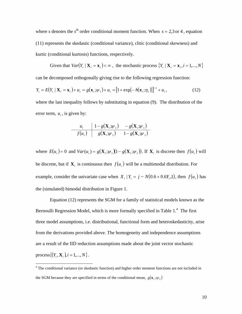
( ) ( ) ( ){ }[ ] iiiiiiiii uhuguYEY +−+=+=+== −111 ;exp1;| ηψ xxxX , (12)

where the last inequality follows by substituting in equation (9). The distribution of the

error term, iu , is given by:

iu ( )1;1 ψig X− ( )1;ψig X− ( )iuf ( )1;ψig X ( )1;1 ψig X−

where ( ) 0=iuE and ( ) ( )( )11 ;1;)( ψψ iii gguVar XX −= . If iX is discrete then ( )iuf will

be discrete, but if iX is continuous then ( )iuf will be a multimodal distribution. For

example, consider the univariate case when ( )1,6.06.0~| iii YNjYX += , then ( )iuf has

the (simulated) bimodal distribution in Figure 1.

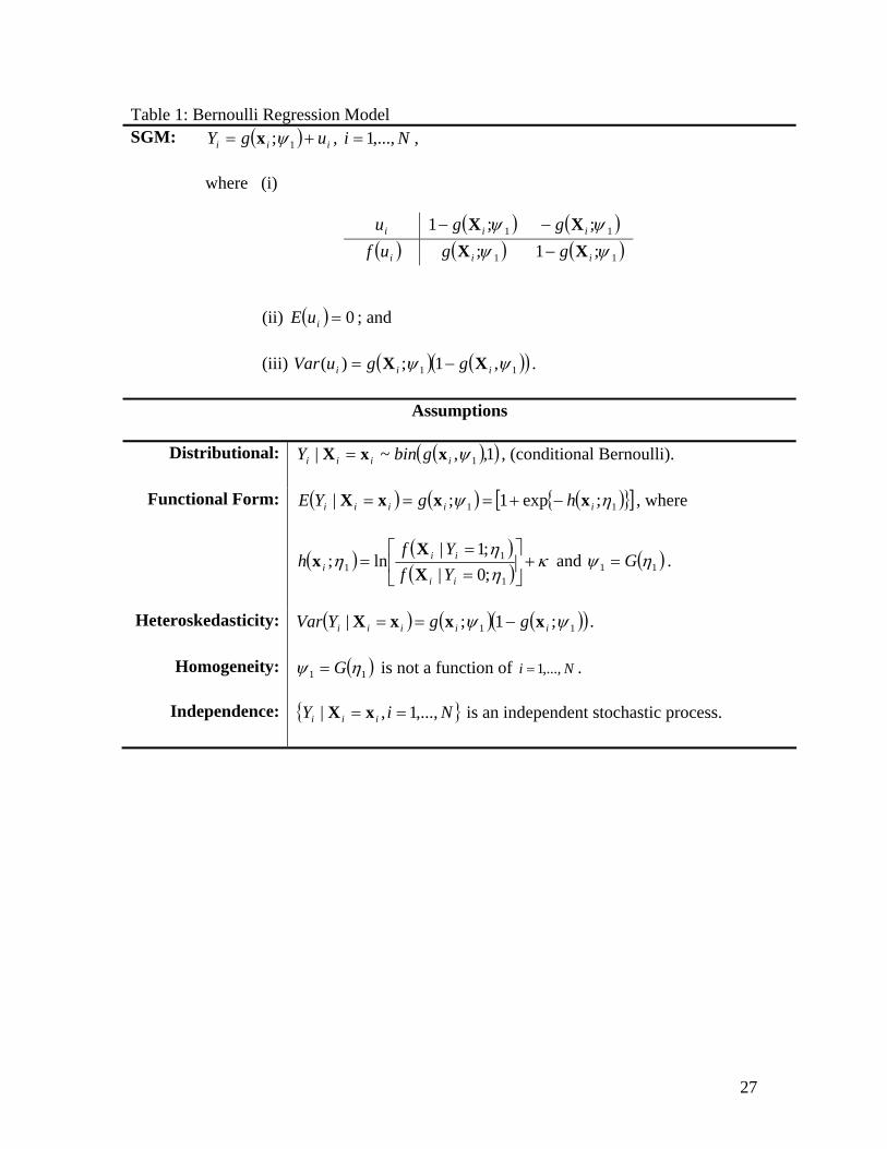
Equation (12) represents the SGM for a family of statistical models known as the

Bernoulli Regression Model, which is more formally specified in Table 1.4 The first

three model assumptions, i.e. distributional, functional form and heteroskedasticity, arise

from the derivations provided above. The homogeneity and independence assumptions

are a result of the IID reduction assumptions made about the joint vector stochastic

process ( ){ }NiY ii ,...,1,, =X .

4 The conditional variance (or skedastic function) and higher order moment functions are not included in

the SGM because they are specified in terms of the conditional mean, ( )1;ψig x

11

The regression function given by equation (12) is similar to the traditional binary

logistic regression model, but above derivations show that it arises naturally from the

joint density function given by equation (1), suggesting it as an obvious candidate for

modeling discrete choice processes when the dependent variable is distributed

Bernoulli(p). Another important observation is that the functional forms for both

( )1;ψig X and ( )1;ηih X are both dependent upon the functional form of ( )1;| ηii Yf X

and in turn the joint distribution of iY and iX .

3. Model Specification

Kay and Little (1987) provide the necessary specifications for ( )1;ηih x

when ikX , , Kk ,...,1= (the explanatory variables) have distributions from the simple

exponential family and are independent conditional on iY of each other. When these

conditions are not met, the model specification becomes more complex. Kay and Little

(1987) provide examples involving sets of random variables with multivariate Bernoulli

and normal distributions, but due to the complexity of dealing with multivariate

distributions they advocate accounting for any dependence between the explanatory

variables by including cross-products of transformations (based on their marginal

distributions) of the explanatory variables. This paper builds on the model specification

work initiated by Kay and Little (1987).

An initial issue concerning specification of BRMs is that ( )1;| ηii Yf X is not

usually known and for many cases cannot be readily derived.5 A potential alternative is to

assume that:

5 For help with such derivations, work by Arnold, Castillo and Sarabia (1999) may be of assistance.

12

( ) ( )( )iiii YfYf 11 ;;| ηη XX = . (13)

In this sense, one is treating the moments of the conditional distribution of iX given iY

as functions of iY . That is ( ) 1,0for ,11 === jjY ji ηη . Lauritzen and Wermuth (1989)

use a similar approach to specify conditional Gaussian distributions, and Kay and Little

(1987) use this approach to specify the logistic regressions models in their paper (see also

Tate, 1954 and Oklin and Tate, 1961).

Table 2 provides the functional forms for ( )1;ψixg needed to obtain a properly

specified BRM with one explanatory variable for a number of different conditional

distributions of the form ( )jiXf ,1;η . Following Kay and Little (1987), all of the cases

examined in Table 2 have index functions that are linear in the parameters. Examples of

conditional distributions that give rise to nonlinear index functions include

when ( )jiXf ,1;η is distributed F, extreme value or logistic. In such cases, one option is to

explicitly specify ( )jiXf ,1;η and estimate the model using equation (9), which can be

difficult numerically due to the inability to reparametricize the model, leaving both 0,1η

and 1,1η in ( )jih ,1;ηx . Another option is to transform iX so that it has one of the

conditional distributions specified in Table 2. To illustrate this latter approach, consider

the following example.

Example 1: Let ( )jiXf ,1;η be a conditional Weibull distribution of the form:

( )⎪⎭

⎪⎬⎫

⎪⎩

⎪⎨⎧

⎟⎟⎠

⎞⎜⎜⎝

⎛−

⋅=

−γ

γ

γ

ααγ

ηj

i

j

ii

XXXf exp;

1

1 , (14)

13

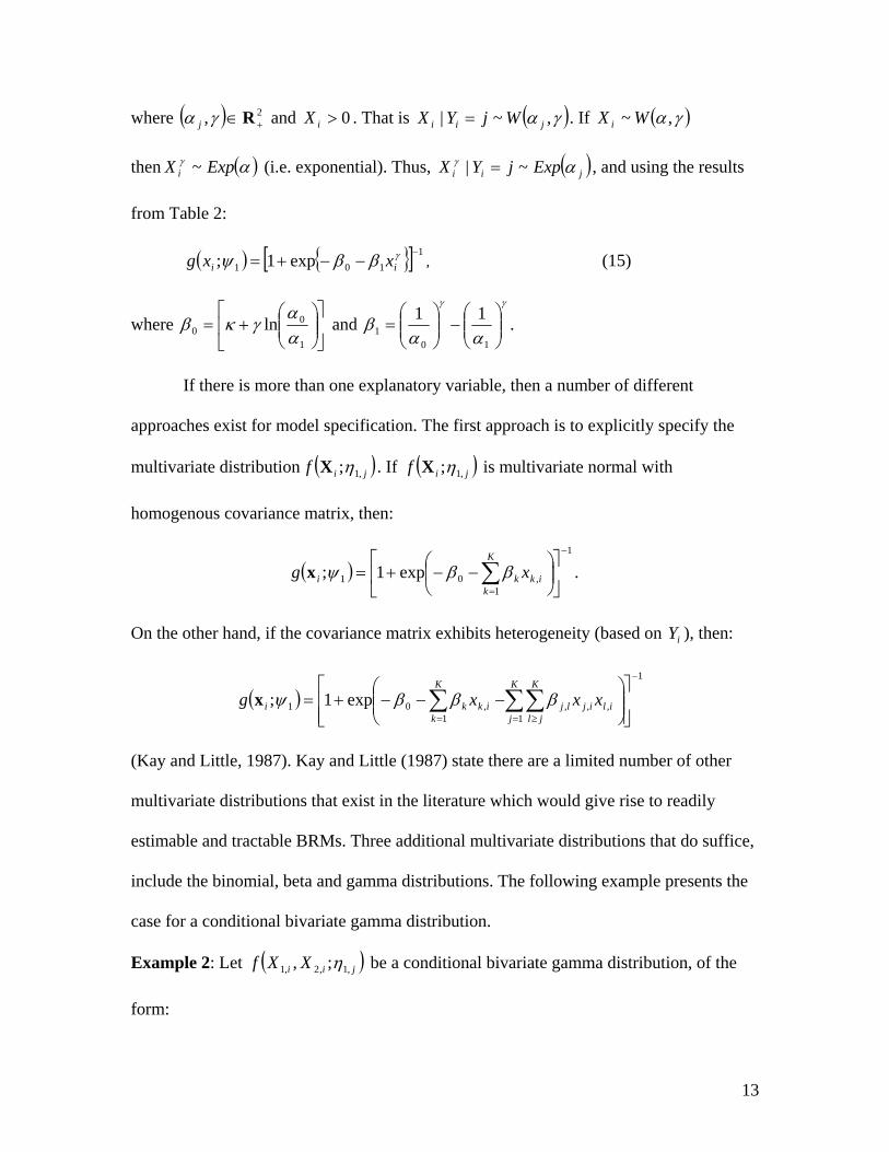
where ( ) 2, +∈Rγα j and 0>iX . That is ( )γα ,~| jii WjYX = . If ( )γα ,~ WX i

then ( )αγ ExpX i ~ (i.e. exponential). Thus, ( )jii ExpjYX αγ ~| = , and using the results

from Table 2:

( ) { }[ ] 1101 exp1; −

−−+= γββψ ii xxg , (15)

where ⎥⎦

⎤⎢⎣

⎡⎟⎟⎠

⎞⎜⎜⎝

⎛+=

1

00 ln

αα

γκβ and γγ

ααβ ⎟⎟

⎠

⎞⎜⎜⎝

⎛−⎟⎟

⎠

⎞⎜⎜⎝

⎛=

101

11 .

If there is more than one explanatory variable, then a number of different

approaches exist for model specification. The first approach is to explicitly specify the

multivariate distribution ( )jif ,1;ηX . If ( )jif ,1;ηX is multivariate normal with

homogenous covariance matrix, then:

( )1

1,01 exp1;

−

=⎥⎦

⎤⎢⎣

⎡⎟⎠

⎞⎜⎝

⎛−−+= ∑

K

kikki xg ββψx .

On the other hand, if the covariance matrix exhibits heterogeneity (based on iY ), then:

( )1

1,,,

1,01 exp1;

−

= ≥= ⎥⎥⎦

⎤

⎢⎢⎣

⎡⎟⎟⎠

⎞⎜⎜⎝

⎛−−−+= ∑∑∑

K

j

K

jlilijlj

K

kikki xxxg βββψx

(Kay and Little, 1987). Kay and Little (1987) state there are a limited number of other

multivariate distributions that exist in the literature which would give rise to readily

estimable and tractable BRMs. Three additional multivariate distributions that do suffice,

include the binomial, beta and gamma distributions. The following example presents the

case for a conditional bivariate gamma distribution.

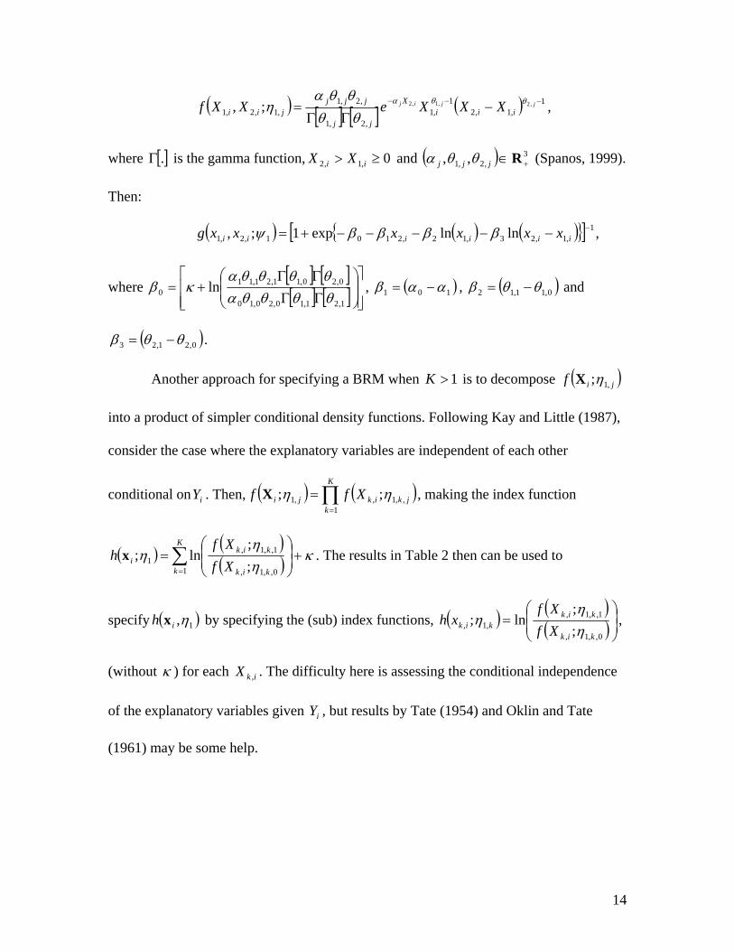
Example 2: Let ( )jii XXf ,1,2,1 ;, η be a conditional bivariate gamma distribution, of the

form:

14

( ) [ ] [ ] ( ) 1,1,2

1,1

,2,1

,2,1,1,2,1

,2,1,2;, −−− −ΓΓ

= jjijiii

X

jj

jjjjii XXXeXXf θθα

θθθθα

η ,

where [ ].Γ is the gamma function, 0,1,2 ≥> ii XX and ( ) 3,2,1 ,, +∈Rjjj θθα (Spanos, 1999).

Then:

( ) ( ) ( ){ }[ ] 1,1,23,12,2101,2,1 lnlnexp1;, −−−−−−+= iiiiii xxxxxxg ββββψ ,

where [ ] [ ][ ] [ ] ⎥

⎥⎦

⎤

⎢⎢⎣

⎡⎟⎟⎠

⎞⎜⎜⎝

⎛

ΓΓ

ΓΓ+=

1,21,10,20,10

0,20,11,21,110 ln

θθθθαθθθθα

κβ , ( )101 ααβ −= , ( )0,11,12 θθβ −= and

( )0,21,23 θθβ −= .

Another approach for specifying a BRM when 1>K is to decompose ( )jif ,1;ηX

into a product of simpler conditional density functions. Following Kay and Little (1987),

consider the case where the explanatory variables are independent of each other

conditional on iY . Then, ( ) ( )∏=

=K

kjkikji Xff

1,,1,,1 ;; ηηX , making the index function

( ) ( )( ) κ

ηη

η +⎟⎟⎠

⎞⎜⎜⎝

⎛= ∑

=

K

k kik

kiki Xf

Xfh

1 0,,1,

1,,1,1 ;

;ln;x . The results in Table 2 then can be used to

specify ( )1,ηih x by specifying the (sub) index functions, ( ) ( )( )⎟

⎟⎠

⎞⎜⎜⎝

⎛=

0,,1,

1,,1,,1, ;

;ln;

kik

kikkik Xf

Xfxh

ηη

η ,

(without κ ) for each ikX , . The difficulty here is assessing the conditional independence

of the explanatory variables given iY , but results by Tate (1954) and Oklin and Tate

(1961) may be some help.

15

If some or none of the explanatory variables are independent conditional on iY ,

then another approach for decomposing ( )jif ,1;ηX is sequential conditioning (Spanos,

1999), i.e.

( ) ( ) ( )∏=

−=K

kjkiikikjiji XXXfXff

2,,1,1,,1,1,1,1 ;,...,|;; ξηηX ,

where jk ,ξ is an appropriate set of parameters. Given the potential complexity of this

approach, it can be combined with the previous approach to reduce the dimensionality

and increase the tractability of the problem. To illustrate this alternative, consider the

following example.

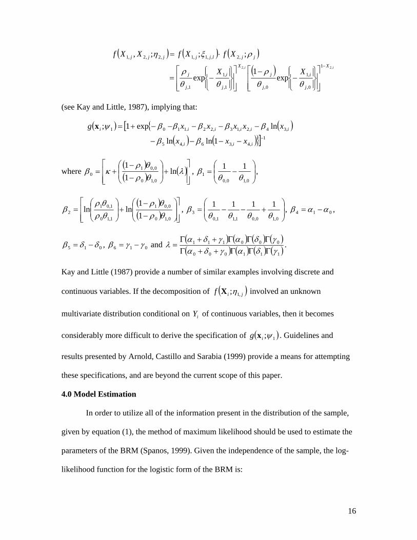
Example 3: Let

( ) ( ) ( )jiijiijiiii XXfXXfXXXXf ,3,4,3,2,2,1,1,4,3,2,1 ;,;,;;,, ηηη ⋅= ,

where iX ,1 and iX ,2 are independent conditional on iY of iX ,3 and iX ,4 . Now assume

that (i) iX ,1 given jYi = is distributed bin(1, jρ ), (ii) iX ,2 given lX i =,1 ( )1,0=l and

jYi = is distributed exponential, i.e.:

( ) ,exp1;,

,1

,,,1,1

⎪⎭

⎪⎬⎫

⎪⎩

⎪⎨⎧−=

lj

i

ljlji

XXf

θθξ

and (iii) iX ,3 and iX ,4 given jYi = are jointly distributed bivariate beta, i.e.:

( ) ( )( ) ( ) ( ) ( )[ ]1

,4,31

,41

,3,3,4,3 1;, −−− −−⋅⋅⎟⎟⎠

⎞⎜⎜⎝

⎛

ΓΓΓ

++Γ= jjj

iiiijjj

jjjjii XXXXXXf γδα

γδαγδα

η ,

where 0,3 ≥iX , 0,4 ≥iX and 1,4,3 ≤+ ii XX for Ni ,...,1= ; ( ) 0,, >jjj γδα for 1,0=j ;

and ( ).Γ is the gamma function (Spanos, 1999). Using these assumptions:

16

( ) ( ) ( )( ) ii X

j

i

j

j

X

j

i

j

j

jjljjjjj

XX

XfXfXXf,2,2 1

0,

,1

0,1,

,1

1,

,2,,1,1,2,2,1

exp1

exp

;;;,−

⎥⎥⎦

⎤

⎢⎢⎣

⎡

⎪⎭

⎪⎬⎫

⎪⎩

⎪⎨⎧−

−

⎥⎥⎦

⎤

⎢⎢⎣

⎡

⎪⎭

⎪⎬⎫

⎪⎩

⎪⎨⎧−=

⋅=

θθρ

θθρ

ρξη

(see Kay and Little, 1987), implying that:

( ) {[ ( )( ) ( )}] 1

,4,36,45

,34,2,13,22.1101

1lnln

lnexp1;−−−−−

−−−−−+=

iii

iiiiii

xxx

xxxxxg

ββ

βββββψx

where ( )( ) ( )

⎥⎥⎦

⎤

⎢⎢⎣

⎡+⎟

⎟⎠

⎞⎜⎜⎝

⎛

−

−+= λ

θρθρ

κβ ln11

0,10

0,010 , ⎟

⎟⎠

⎞⎜⎜⎝

⎛−=

0,10,01

11θθ

β ,

( )( ) ⎥

⎥⎦

⎤

⎢⎢⎣

⎡⎟⎟⎠

⎞⎜⎜⎝

⎛

−

−+⎟

⎟⎠

⎞⎜⎜⎝

⎛=

0,10

0,01

1,10

1,012 1

1lnln

θρθρ

θρθρ

β , ⎟⎟⎠

⎞⎜⎜⎝

⎛+−−=

0,10,01,11,03

1111θθθθ

β , 014 ααβ −= ,

015 δδβ −= , 016 γγβ −= and ( ) ( ) ( ) ( )( ) ( ) ( ) ( )111000

000111

γδαγδαγδαγδα

λΓΓΓ++ΓΓΓΓ++Γ

= .

Kay and Little (1987) provide a number of similar examples involving discrete and

continuous variables. If the decomposition of ( )jif ,1;ηX involved an unknown

multivariate distribution conditional on iY of continuous variables, then it becomes

considerably more difficult to derive the specification of ( )1;ψig x . Guidelines and

results presented by Arnold, Castillo and Sarabia (1999) provide a means for attempting

these specifications, and are beyond the current scope of this paper.

4.0 Model Estimation

In order to utilize all of the information present in the distribution of the sample,

given by equation (1), the method of maximum likelihood should be used to estimate the

parameters of the BRM (Spanos, 1999). Given the independence of the sample, the log-

likelihood function for the logistic form of the BRM is:

17

( )( ) ( )( )( ) ( ) ( )( )( )[ ]∑=

−−+=N

iiiii hgyhgyL

111 ;1ln1;ln,;ln ψψϕ xxxy , (16)

where ( ).g is the logistic cdf and ( ).,.h is written as a function of 1ψ , the parameters of

interest. Now let ih∂ denote the gradient of ( )1;ψih x with respect to the vector 1ψ

(e.g.β ), ih2∂ the Hessian, and ( ).g ′ the logistic probability density function. Then:

( )( ) ( )( )( )( ) ( )( )( ) ( )( )∑

=⎥⎦

⎤⎢⎣

⎡∂′⎟⎟

⎠

⎞⎜⎜⎝

⎛−

−=

∂∂ N

iii

ii

ii hghghg

hgyL1

111

1

1

;;1;

;,;ln hxxx

xxy ψψψ

ψψϕ , and

( )( ) ( )( )( )( ) ( )( )( ) ( )( )( ) ( )( )

( )( )( )( ) ( )( )( ) ( )( )( )( ) ( )( )( )( ) .;;

;1;;

;;1;

;,,ln

1

21

T1

11

1

1

T21

2

11

1

11

2

∑

∑

=

=

⎥⎦

⎤⎢⎣

⎡∂+∂∂′⎟⎟

⎠

⎞⎜⎜⎝

⎛−

−+

⎥⎥⎦

⎤

⎢⎢⎣

⎡∂∂′⎟⎟

⎠

⎞⎜⎜⎝

⎛−

−−=

′∂∂∂

N

iiiiii

ii

ii

N

iiii

ii

ii

hghghghg

hgy

hghghg

hgyL

hxhhxxx

x

hhxxx

xxy

ψψψψ

ψ

ψψψ

ψψψ

ϕ

When ( )1;ηih x is nonlinear in the parameters estimation becomes more difficult, because

the likelihood function may no longer be globally concave and many computer routines

only estimate logistic regression models with index functions linear in the parameters

(Train, 2003). In these cases, the researcher may need to write their own code and use a

number of different algorithms to estimate the model. The asymptotic properties of

consistency and asymptotic normality of the MLE estimates follow if certain regularity

conditions are satisfied (see Gourieroux, 2000 and Spanos, 1999).

5. Simulation

A significant benefit of using the probabilistic reduction approach for developing

the BRM is that it provides a mechanism for randomly generating the vector stochastic

process, ( ){ }NiY ii ,...,1,, =X using the relationship given by equation (4) for simulations

involving the BRM. The process involves performing two steps:

18

Step 1: Generate a realization of the stochastic process { }NiYi ,...,1, = using a binomial

random number generator.

Step 2: Using ( )jif ,1;ηX generate a realization of the vector stochastic process,

{ }Nii ,...,1, =X using appropriate random number generators with the parameters given

by 0,1,1 ηη =j when 0=iY and 1,1,1 ηη =j when 1=iY .

It should be noted that no a priori theoretical interpretation is imposed on the generation

process, it is purely statistical in nature.6 Furthermore, the parameters 1ψ can be easily

determined from the parameters j,1η , via ( )0,11,11 ,ηηψ G= when conducting simulations.

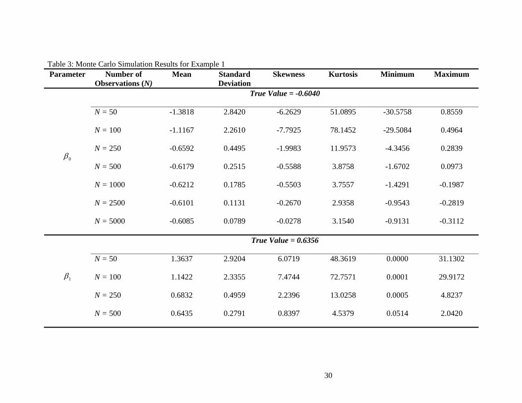
To illustrate, consider the BRM given in Example 1. Let ( )1,6.0~ binYi and

jYX ii =| have a conditional Weibull distribution with 10 =α , 4.11 =α and 3=γ . In

this situation, the mapping ( )0,11,11 ,ηηψ G= given in Example 1 gives 6040.00 −=β ,

6356.01 =β and 3=γ for the parameters of the regression function given by equation

(15). A Monte Carlo simulation using the above two-step procedure for randomly

generating a binary choice process was used to examine the asymptotic properties of the

parameters 0β , 1β and γ . A random sample of iY ( 6.0=p ) was generated 1000 times

and then was used to generate iX 100 times using equation (14) for

5000and 2500,1000,500,250,100,50=N . For each run, the regression equation given

by equation (15) was estimated using the log likelihood function given by equation (16)

6 This generation procedure is in contrast to procedures assuming the existence of an unobservable latent

stochastic process (see Train, 2003).

19

and a derivative-free algorithm developed by Nelder and Mead (1965).7 The results of the

simulation are reported in Table 3. Given the convergence of the mean to the true value,

the decreasing standard errors, and convergence of the skewness and kurtosis towards 0

and 3 respectively, as N increases, it would seem that there is evidence for concluding

that 0β , 1β and γ are consistent and asymptotically normal.

6. Empirical Example

Data was obtained from Al-Hmoud and Edwards (2004) from a study examining

private sector participation in the water and sanitation sector of developing countries.

Using there data a model was constructed examining this participation based on four

explanatory factors. The dependent variable, total private investment (Y ), was binary,

taking a value of ‘1’ if there was private investment in a given year and ‘0’ otherwise. Of

the four explanatory variables used in the model, two were binary and two were

continuous. The two binary variables were low renewable water resources ( 3X ) and

government effectiveness ( 4X ). The two continuous variables were per capita GDP ( 1X )

and percent urban population growth ( 2X ). The dataset contained 149 observations for

39 countries from 1996 to 2001, but data was not available for all countries for all years,

resulting in an unbalanced panel (Al-Hmoud and Edwards, 2004).

Given that Y is distributed Bernoulli, a BRM was chosen to model private sector

participation in developing countries in the water and sanitation sector. To examine how

7 It was found that this algorithm provided the best convergence properties for the given problem. A

potential problem with index functions nonlinear in the parameters is the difficulty algorithms using

derivatives and Hessians may have in finding an optimal solution due to potentially highly nonlinear or

large relatively flat regions of the objective surface.

20

to proceed with model specification, the sample conditional correlation matrix given

Y was estimated using the sample correlation coefficients of the residuals from

appropriate regressions of the explanatory variables on Y .8 The sample conditional

correlation matrix was:

⎟⎟⎟⎟⎟

⎠

⎞

⎜⎜⎜⎜⎜

⎝

⎛

−−

−−−−

00.119.019.054.019.000.152.011.019.052.000.145.0

54.011.045.000.1

,

which provided no determination on how to decompose ( )jiiii XXXXf ,1,4,3,2,1 ;,,, η into

independent components. Thus, sequential conditioning was used to give:

( ) ( ) ( )jiilkjiijiiii XXfXXfXXXXf q;,;,;,,, ,4,3,,,1,2,1,1,4,3,2,1 ⋅′= ηη , (17)

where ( )lXkXjY iiilkj ====′ ,4,31,,,1 ,,ηη and

( ) ( )( ) ( ) ( ) iiiiiiii XXj

XXj

XXj

XXjjii qqqqXXf ,4.3,4,3,4,3,4.3

1,1,1

1,0,1

0,1,11

0,0,,4,3 ;, −−−−=q , (18)

where 11,1,1,0,0,1,0,0, =+++ jjjj qqqq . That is, equation (18) is a multivariate

Bernoulli( jq ) distribution conditional on jYi = .

After taking account of the heterogeneity in the continuous explanatory variables,

it was assumed that iX ,1 and iX ,2 were jointly distributed bivariate normal conditional on

lXkXjY iii === ,4,3 and , for 1,0,, =lkj , i.e.

( ) ( ) ( ) ( ) ,21exp2;, ,,

1,,,,

21

,,1

,,,1,2,1⎭⎬⎫

⎩⎨⎧ −Σ′−−Σ=′ −−−

lkjilkjlkjilkjlkjii XXf µµπη XX (19)

8 For the binary explanatory variables, appropriate logistic regression models were estimated, while for the

continuous explanatory variables normal linear regression models were used.

21

where ( )′= iii XX ,2,1 ,X , ( )′= lkjlkjlkj ,,,2,,,1,, ,µµµ is a vector of conditional means, lkj ,,Σ is

the conditional covariance matrix, and . signifies the determinant operator. Given

equation (18), this implies that:

( ) ( )[ ]( )( )

( )[ ] ( )

( )[ ]( )

( )[ ] (20) .;,

;,

;,

;,;,,,

,4,3

,4,3

,4,3

,4,3

1,1,,1,2,11,1,

11,0,,1,2,11,0,

10,1,,1,2,10,1,

110,0,,1,2,10,0,,1,4,3,2,1

ii

ii

ii

ii

XXjiij

XXjiij

XXjiij

XXjiijjiiii

XXfq

XXfq

XXfq

XXfqXXXXf

η

η

η

ηη

′⋅

×′⋅

×′⋅

×′⋅=

−

−

−−

Plugging equation (20) into ( )1;ηih x and computing ( )jG ,11 ηψ = :

( )

(21) ,

;

,4,32,223

,4,3,2,122,4,32,121,4,3,220,4,3,119

,42,218,4,2,1174

2,116,3

2,215,3,2,114

,32,113,4,312,4,211,4,110,3,29,3,18

2,27,2,16

2,15,44,33,22,1101

iii

iiiiiiiiiiiii

iiiiiiiiiii

iiiiiiiiiiii

iiiiiiiii

xxx

xxxxxxxxxxxxx

xxxxxxxxxxxx

xxxxxxxxxxxx

xxxxxxxxh

β

ββββ

βββββ

ββββββ

ββββββββψ

++++

+++++

++++++

++++++++=x

which when plugged into equation (9) provides an estimable BRM. If Σ=Σ lkj ,, , then all

the terms involving 2,1 ix , ii xx ,2,1 and 2

,2 ix would disappear, but this was not the case.9

Since the index function given by equation (21) is linear in the parameters,

standard computer software packages with logistic regression models, were used to

estimate the corresponding BRM. Estimation results for the logistic regression model

using equation (21) and a more common specification found in the applied literature:

( ) iiiii xxxxh ,44,33,22,1101; βββββψ ++++=x , (22)

9 Results of these analyses using the data are available from the authors upon request.

22

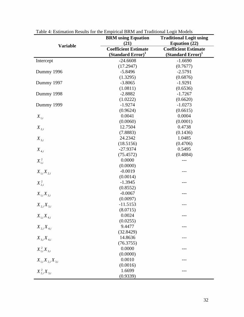
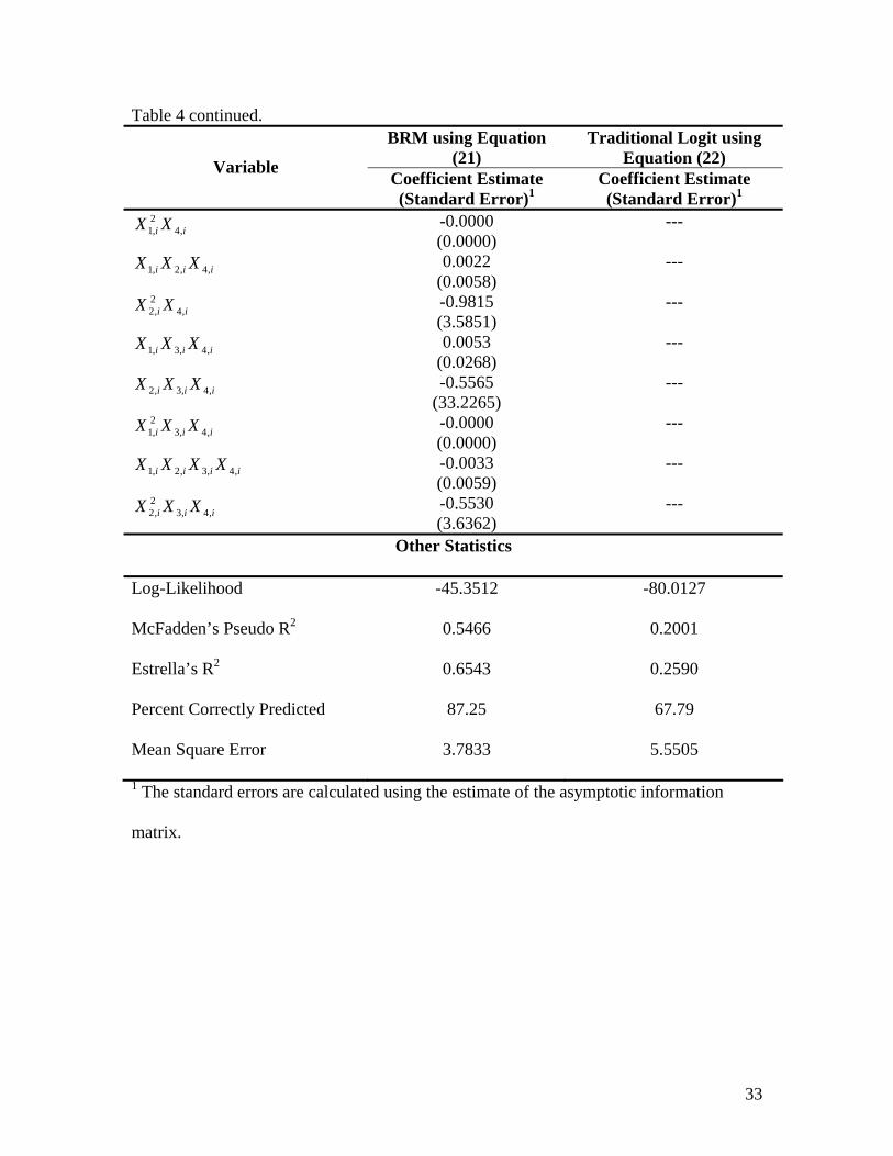
are presented in Table 4. Misspecification testing results for the BRM using equation (21)

indicated the presence of heterogeneity across years, so fixed effects (using dummy

variables) for the years 1996-1999 were incorporated into both models.10

The two models were compared using a likelihood ratio test, with the null

hypothesis being that the more common specification of the logit model using equation

(22) with fixed effects across time was correct. The computed likelihood ratio test

statistic was 69.3229 with an associated p-value of 0.0000, indicating that the more

common formulation of the logistic regression model is misspecified. Further evidence

that the BRM using equation (22) was superior to the more common specification of the

logistic regression model is given by the higher R2 values, higher within-sample

prediction and lower mean square error.11

7. Conclusion

The latent variable approach and the transformational approach for specifying

statistical models with binary dependent variables can result in statistical

misspecification. Both approaches do not explicitly recognize that the functional form of

( )iiiYE xX =| depends on ( )1;| ηjYf ii =X and in turn the existence of ( )ϕ;, iiYf X .

Using the probabilistic reduction approach and results derived by Kay and Little (1987),

10 A likelihood ratio test was conducted in a Fisher testing framework to examine the BRM without fixed

effects across time (see Spanos, 1999). The null hypothesis was no fixed effects and the likelihood test

statistic was 34.1369 with an association p-value of 0.00001, indicating no support for the null hypothesis.

Heterogeneity across regions was tested as well, but no evidence of this type of heterogeneity was found.

11 Additional misspecification tests for functional form and dependence indicated that the functional form

was not misspecified, but there may exist temporal and/or spatial dependence in the data. These tests and

results are available from the authors upon request and will be explored further in a future paper.

23

this relationship is formally defined to derive the Bernoulli Regression Model. While

specification of these models can be difficult at times, examination of the sample

conditional correlation matrix of the explanatory variables given iY can help determine

plausible decompositions of ( )1;| ηjYf ii =X to arrive at operational BRMs.

Furthermore, the model assumptions shown in Table 1 can be tested to verify that the

BRM obtained is statistically adequate, thereby allowing the model to provide reliable

statistical inferences and predictions. The theoretical and empirical examples provide

evidence that the common use of logit and probit models with linear index functions both

in the parameters and variables are suspect when the underlying model assumptions have

not been verified.

The Bernoulli Regression Model can provide a parsimonious description of the

probabilistic structure of conditional binary choice process being examined and imposes

no a priori theoretical or ad hoc restrictions (or assumptions) upon the model, thereby

providing a theory-free statistical model of the conditional binary choice process being

examined. As noted by Spanos (1995), this freedom allows the modeler to conduct

statistical inferences (if the statistical assumptions made about the underlying stochastic

process are appropriate) that can be used to examine if the theory in question can account

for the systematic information in the observed data.

24

References

1. Al-Hmoud, R.B. and J. Edwards. “A Means to an End: Studying the Existing

Environment for Private Sector Participation in the Water and Sanitation Sector.”

Working Paper. Department of Economics and Geography, Texas Tech University,

Lubbock Texas, 2004.

2. Arnold, B.C., E. Castillo and J.M. Sarabia. Conditional Specification of Statistical

Models. New York, NY: Springer Verlag, 1999.

3. Arnold, B.C. and S.J. Press. “Compatible Conditional Distributions.” Journal of the

American Statistical Association. 84(March, 1989): 152 – 156.

4. Coslett, S.R. “Distribution-Free Maximum Likelihood Estimator of the Binary Choice

Model.” Econometrica. 51(May 1983): 765 – 782.

5. Cox, D.R. and N. Wermuth. “Response Models for Mixed Binary and Qualitative

Variables. Biometrika. 79(1992): 441 – 461.

6. Fahrmeir, L. and G. Tutz. Multivariate Statistical Modeling Based on Generalized

Linear Models. New York: Springer-Verlag, 1994.

7. Gourieroux, C. Econometrics of Qualitative Dependent Variables. Cambridge, UK:

Cambridge University Press, 2000.

8. Kay, R. and S. Little. “Transformations of the Explanatory Variables in the Logistic

Regression Model for Binary Data.” Biometrika. 74(September, 1987): 495 – 501.

9. Keane, M.P. “Current Issues in Discrete Choice Modeling.” Marketing Letters.

8(1997): 307 – 322.

25

10. Lauritzen, S.L. and N. Wermuth. “Graphical Models for Association Between

Variables, Some Which Are Qualitative and Some Quantitative.” Annals of Statistics.

17(1989): 31 – 57.

11. Maddala, G.S. Limited Dependent and Qualitative Variables in Econometrics.

Cambridge, UK: Cambridge University Press, 1983.

12. Nelder, J.A. and R. Mead. “A Simplex Method for Function Minimization.”

Computer Journal. 7(1965): 308 – 313.

13. Nelder, J.A. and R.W.M. Wedderburn. “Generalized Linear Models.” Journal of the

Royal Statistical Society, Series A (General). 3(1972): 370 – 384.

14. Oklin, I. and R.F. Tate. “Multivariate Correlation Models with Mixed Discrete and

Continuous Variables.” The Annals of Mathematical Statisitcs. 32(June, 1961): 448 –

465.

15. Powers, D.A. and Y. Xie. Statistical Methods for Categorical Data Analysis. San

Deigo, CA: Academic Press, 2000.

16. Small, C.G. and D.L. McLeish. Hilbert Space Methods in Probability and Statistical

Inference. New York: John Wiley and Sons, Inc., 1994.

17. Spanos, A. “On Theory Testing In Econometrics: Modeling with Nonexperimental

Data.” Journal of Econometrics. 67(1995): 189 – 226.

18. Spanos, A. Probability Theory and Statistical Inference: Econometric Modeling with

Observational Data. Cambridge, UK: Cambridge University Press, 1999.

19. Spanos, A. Statistical Foundations of Econometrics Modeling. Cambridge, UK:

Cambridge University Press, 1986.

26

20. Tate, R.F. “Correlation Between a Discrete and a Continuous Variable. Point-Biserial

Correlation.” The Annals of Mathematical Statistics. 25(September, 1954): 603 – 607.

21. Train, K.E. Discrete Choice Methods with Simulation. Cambridge, UK: Cambridge

University Press, 2003.

27

Table 1: Bernoulli Regression Model SGM: ( ) iii ugY += 1;ψx , Ni ,...,1= ,

where (i)

iu ( )1;1 ψig X− ( )1;ψig X− ( )iuf ( )1;ψig X ( )1;1 ψig X−

(ii) ( ) 0=iuE ; and

(iii) ( ) ( )( )11 ,1;)( ψψ iii gguVar XX −= .

Assumptions

Distributional: ( )( )1,,~| 1ψiiii gbinY xxX = , (conditional Bernoulli).

Functional Form: ( ) ( ) ( ){ }[ ]11 ;exp1;| ηψ iiiii hgYE xxxX −+=== , where

( ) ( )( ) κ

ηη

η +⎥⎦

⎤⎢⎣

⎡==

=1

11 ;0|

;1|ln;

ii

iii Yf

Yfh

XX

x and ( )11 ηψ G= .

Heteroskedasticity: ( ) ( ) ( )( )11 ;1;| ψψ iiiii ggYVar xxxX −== .

Homogeneity: ( )11 ηψ G= is not a function of Ni ,...,1= .

Independence: { }NiY iii ,...,1,| == xX is an independent stochastic process.

28

Table 2: Specification of ( )1;ηixg with one explanatory variable and conditional distribution, ( )jiXf ,1;η , for 1,0=j . Distribution of

iX given iY ( )=jiXf ,1;η 2 ( ) =1;ψixg

Beta1 ( )[ ]jj

iijj XX

γα

γα

,1 11

B

−− −, where

( ) .10 and , 2 ≤≤∈ + ijj XRγα

( ) ( ){ }[ ] 1210 1lnlnexp1 −−+++ ii xx βββ , where

[ ][ ] ( ) ( ). and ,

,,

ln 01201111

000 γγβααβ

γαγα

κβ −=−=⎥⎥⎦

⎤

⎢⎢⎣

⎡⎟⎟⎠

⎞⎜⎜⎝

⎛+=

BB

Binomial1 ( ) ii Xnj

Xj

iXn −−⎟⎟⎠

⎞⎜⎜⎝

⎛θθ 1 , where

,...3,2,1 and 1,0,10 ==<< nX ijθ

{ }[ ] 110exp1 −−−+ ixββ , where

.11

lnln and 11

ln0

1

0

11

0

10 ⎟⎟

⎠

⎞⎜⎜⎝

⎛−−

−⎟⎟⎠

⎞⎜⎜⎝

⎛=

⎥⎥⎦

⎤

⎢⎢⎣

⎡⎟⎟⎠

⎞⎜⎜⎝

⎛−−

+=θθ

θθ

βθθ

κβ n

Chi-square

⎭⎬⎫

⎩⎨⎧−

⎥⎥⎦

⎤

⎢⎢⎣

⎡Γ

−−

2exp

2

2 22

2i

v

ij

v

XX

v

jj

, where

. and ,...3,2,1 +∈= Rxv

{ }[ ] 110exp1 −−−+ ixββ , where

( ) . 2

and

2

2ln2ln

201

11

0

100

vvv

vvv −

=

⎥⎥⎥⎥⎥

⎦

⎤

⎢⎢⎢⎢⎢

⎣

⎡

⎟⎟⎟⎟⎟

⎠

⎞

⎜⎜⎜⎜⎜

⎝

⎛

⎥⎦

⎤⎢⎣

⎡Γ

⎥⎦

⎤⎢⎣

⎡Γ

+⎟⎟⎠

⎞⎜⎜⎝

⎛ −+= βκβ

Exponential ⎪⎭

⎪⎬⎫

⎪⎩

⎪⎨⎧−

j

i

j

Xθθ

exp1 , where

. and ++ ∈∈ RR ij Xθ

{ }[ ] 110exp1 −−−+ ixββ , where

.11 and ln10

01

00 ⎟⎟

⎠

⎞⎜⎜⎝

⎛−=

⎥⎥⎦

⎤

⎢⎢⎣

⎡+⎟⎟

⎠

⎞⎜⎜⎝

⎛=

θθβκ

θθ

β

Gamma1

[ ] ⎪⎭

⎪⎬⎫

⎪⎩

⎪⎨⎧−⎟

⎟⎠

⎞⎜⎜⎝

⎛

Γ

−

j

i

j

i

jj

XX j

γγαγ

α

exp11

, where

( ) . and , 2++ ∈∈ RR ijj Xγα

( ){ }[ ] 1210 lnexp1 −+++ ii xx βββ , where

[ ][ ] ( ) ( ) ( ) ( ) ( ). and 11,ln1ln1ln 012

1011100

11

000 ααβ

γγβγαγα

αγαγ

κβ −=⎟⎟⎠

⎞⎜⎜⎝

⎛−=

⎥⎥⎦

⎤

⎢⎢⎣

⎡−−−+⎟⎟

⎠

⎞⎜⎜⎝

⎛ΓΓ

+=

Geometric 1)1( −− iXjj θθ , where

,...3,2,1 and 10 =≤≤ ij Xθ

{ }[ ] 110exp1 −−−+ ixββ , where

.11

ln and 11

lnln0

11

0

1

0

10 ⎟⎟

⎠

⎞⎜⎜⎝

⎛−−

=⎥⎥⎦

⎤

⎢⎢⎣

⎡⎟⎟⎠

⎞⎜⎜⎝

⎛−−

−⎟⎟⎠

⎞⎜⎜⎝

⎛+=

θθ

βθθ

θθ

κβ

29

Table 2 continued.

Logarithmic ,⎟⎟

⎠

⎞

⎜⎜

⎝

⎛

i

Xj

j X

iθα where

( )[ ] ,...3,2,1X and 10,1ln i1 =<<−−= −

jjj θθα

{ }[ ] 110exp1 −−−+ ixββ , where

.ln and ln0

11

0

10 ⎟⎟

⎠

⎞⎜⎜⎝

⎛=

⎥⎥⎦

⎤

⎢⎢⎣

⎡⎟⎟⎠

⎞⎜⎜⎝

⎛+=

θθ

βαα

κβ

Log-Normal ( )( )⎪⎭

⎪⎬⎫

⎪⎩

⎪⎨⎧ −−⋅

2

2

2

lnexp

211

j

ji

ji

XX σ

µ

πσ, where

. and , 2 RRR ∈∈∈ + ijj Xσµ

( )( ){ }[ ] 12210 ln)ln(exp1

−+++ ii xx βββ , where

.2

12

1 and ,22

ln 21

20

220

021

112

1

21

20

20

1

00 ⎟

⎟⎠

⎞⎜⎜⎝

⎛−=⎟

⎟⎠

⎞⎜⎜⎝

⎛−=

⎥⎥⎦

⎤

⎢⎢⎣

⎡⎟⎟⎠

⎞⎜⎜⎝

⎛−+⎟⎟

⎠

⎞⎜⎜⎝

⎛+=

σσβ

σµ

σµβ

σµ

σµ

σσκβ

Normal1 ( )

⎪⎭

⎪⎬⎫

⎪⎩

⎪⎨⎧

−− 222

1exp1ji

jj

X µσπσ

, where

. and , 2 RRR ∈∈∈ + ijj Xσµ

{ }[ ] 12210exp1

−+++ ii xx βββ , where

.2

12

1 and ,22

ln 21

20

220

021

112

1

21

20

20

1

00 ⎟

⎟⎠

⎞⎜⎜⎝

⎛−=⎟

⎟⎠

⎞⎜⎜⎝

⎛−=

⎥⎥⎦

⎤

⎢⎢⎣

⎡⎟⎟⎠

⎞⎜⎜⎝

⎛−+⎟⎟

⎠

⎞⎜⎜⎝

⎛+=

σσβ

σµ

σµβ

σµ

σµ

σσκβ

Pareto 10

−− jjij Xx θθθ , where

. and 0, 00 xXx ij ≥>∈ +Rθ

( ){ }[ ] 110 lnexp1 −−−+ ixββ , where

( ) ( ) ( ).1010010

10 and lnln θθβθθ

θθ

κβ −=⎥⎥⎦

⎤

⎢⎢⎣

⎡−+⎟⎟

⎠

⎞⎜⎜⎝

⎛+= x

Poisson1 !i

Xj

X

e ijθθ−

, where

,...3,2,1 and 0 => ij Xθ

{ }[ ] 110exp1 −−−+ ixββ , where

[ ] .ln and 0

11`00 ⎟⎟

⎠

⎞⎜⎜⎝

⎛=−+=

θθ

βθθκβ

1 Source: Kay and Little (1987).

2 Source: Spanos (1999). [ ]B represents the beta function and [ ]Γ represents the gamma function.

30

Table 3: Monte Carlo Simulation Results for Example 1 Parameter Number of

Observations (N) Mean Standard

Deviation Skewness Kurtosis Minimum Maximum

True Value = -0.6040

N = 50 -1.3818 2.8420 -6.2629 51.0895 -30.5758 0.8559

N = 100 -1.1167 2.2610 -7.7925 78.1452 -29.5084 0.4964

N = 250 -0.6592 0.4495 -1.9983 11.9573 -4.3456 0.2839

N = 500 -0.6179 0.2515 -0.5588 3.8758 -1.6702 0.0973

N = 1000 -0.6212 0.1785 -0.5503 3.7557 -1.4291 -0.1987

N = 2500 -0.6101 0.1131 -0.2670 2.9358 -0.9543 -0.2819

0β

N = 5000 -0.6085 0.0789 -0.0278 3.1540 -0.9131 -0.3112

True Value = 0.6356

N = 50 1.3637 2.9204 6.0719 48.3619 0.0000 31.1302

N = 100 1.1422 2.3355 7.4744 72.7571 0.0001 29.9172

N = 250 0.6832 0.4959 2.2396 13.0258 0.0005 4.8237

1β

N = 500 0.6435 0.2791 0.8397 4.5379 0.0514 2.0420

31

Table 3 continued. Parameter Number of

Observations (N) Mean Standard

Deviation Skewness Kurtosis Minimum Maximum

N = 1000 0.6506 0.1992 0.7351 4.1469 0.1581 1.6016

N = 2500 0.6421 0.1269 0.3445 2.9474 0.2739 1.0701 1β

N = 5000 0.6376 0.0895 0.0660 2.9984 0.3223 0.9763

True Value = 3.0

N = 50 4.6698 4.3463 2.4179 11.6444 -6.6156 36.2235

N = 100 4.1471 3.5111 2.6295 13.0030 0.0824 28.0070

N = 250 3.5300 1.7017 2.5781 16.4192 0.4513 17.7591

N = 500 3.2363 0.9155 1.2591 6.8497 1.1333 9.1500

N = 1000 3.0825 0.5811 0.6526 4.3230 1.6281 6.1177

N = 2500 3.0361 0.3655 0.2861 2.9450 2.1125 4.2341

γ

N = 5000 3.0250 0.2609 0.3726 3.2808 2.2855 4.1462

32

Table 4: Estimation Results for the Empirical BRM and Traditional Logit Models BRM using Equation

(21) Traditional Logit using

Equation (22) Variable Coefficient Estimate (Standard Error)1

Coefficient Estimate (Standard Error)1

Intercept -24.6608 (17.2947)

-1.6690 (0.7677)

Dummy 1996 -5.8496 (1.3295)

-2.5791 (0.6876)

Dummy 1997 -3.8065 (1.0811)

-1.9291 (0.6536)

Dummy 1998 -2.8882 (1.0222)

-1.7267 (0.6620)

Dummy 1999 -1.9274 (0.9624)

-1.0273 (0.6615)

iX ,1 0.0041 (0.0060)

0.0004 (0.0001)

iX ,2 12.7504 (7.8883)

0.4738 (0.1436)

iX ,3 24.2342 (18.5156)

1.0485 (0.4706)

iX ,4 -27.9374 (75.4572)

0.5495 (0.4884)

2,1 iX 0.0000

(0.0000) ---

ii XX ,2,1 -0.0019 (0.0014)

---

2,2 iX -1.3945

(0.8552) ---

ii XX ,3,1 -0.0067 (0.0097)

---

ii XX ,3,2 -11.5153 (8.0715)

---

ii XX ,4,1 0.0024 (0.0255)

---

ii XX ,4,2 9.4477 (32.8429)

---

ii XX ,4,3 14.8636 (76.3755)

---

ii XX ,32,1 0.0000

(0.0000) ---

iii XXX ,3,2,1 0.0010 (0.0016)

---

ii XX ,32,2 1.6699

(0.9339) ---

33

Table 4 continued. BRM using Equation

(21) Traditional Logit using

Equation (22) Variable Coefficient Estimate (Standard Error)1

Coefficient Estimate (Standard Error)1

ii XX ,42,1 -0.0000

(0.0000) ---

iii XXX ,4,2,1 0.0022 (0.0058)

---

ii XX ,42,2 -0.9815

(3.5851) ---

iii XXX ,4,3,1 0.0053 (0.0268)

---

iii XXX ,4,3,2 -0.5565 (33.2265)

---

iii XXX ,4,32,1 -0.0000

(0.0000) ---

iiii XXXX ,4,3,2,1 -0.0033 (0.0059)

---

iii XXX ,4,32,2 -0.5530

(3.6362) ---

Other Statistics

Log-Likelihood -45.3512 -80.0127

McFadden’s Pseudo R2 0.5466 0.2001

Estrella’s R2 0.6543 0.2590

Percent Correctly Predicted 87.25 67.79

Mean Square Error 3.7833 5.5505

1 The standard errors are calculated using the estimate of the asymptotic information

matrix.

34

Figure 1: Simulated Density Plot for a Bernoulli Regression Model with One Explanatory

Variable Conditionally Distributed Normal Given jYi = .