statistical methods for testing genetic pleiotropy
TRANSCRIPT

1
Statistical Methods for Testing Genetic Pleiotropy
Daniel J. Schaid1, Xingwein Tong3,
Beth Larrabee1, Richard B. Kennedy2, Gregory A. Poland2, Jason P. Sinnwell1
1) Dept. Health Sciences Research and 2) Mayo Clinic Vaccine Research Group, Mayo
Clinic, Rochester, MN, USA; 3) School of Statistics, Beijing Normal University,
Beijing, China.
Abstract
Genetic pleiotropy is when a single gene influences more than one trait. Detecting
pleiotropy and understanding its causes can improve the biological understanding of a gene in
multiple ways, yet current multivariate methods to evaluate pleiotropy test the null hypothesis
that none of the traits are associated with a variant; departures from the null could be driven by
just one associated trait. A formal test of pleiotropy should assume a null hypothesis that one or
fewer traits are associated with a genetic variant. For the special case of two traits, one can
construct this null hypothesis based on the intersection-union test (IU) [Silvapulle and Sen 2004],
which rejects the null hypothesis only if the null hypotheses of no association for both traits are
rejected. To allow for more than two traits, we developed a new likelihood ratio test for
pleiotropy. We then extended the testing framework to a sequential approach to test the null
Genetics: Early Online, published on August 15, 2016 as 10.1534/genetics.116.189308
Copyright 2016.

2
hypothesis that 1k + traits are associated, given that the null of k traits are associated was
rejected. This provides a formal testing framework to determine the number of traits associated
with a genetic variant, while accounting for correlations among the traits. By simulations, we
illustrate the Type-I error rate and power of our new methods, describe how they are influenced
by sample size, the number of traits, and the trait correlations, and apply the new methods to
multivariate immune phenotypes in response to smallpox vaccination. Our new approach
provides a quantitative assessment of pleiotropy, enhancing current analytic practice.
Key Words: constrained model, likelihood ratio test, multivariate analysis, seemingly unrelated
regression, sequential testing

3
Introduction
Genetic pleiotropy is when a single gene influences more than one trait. Detecting
pleiotropy, and understanding its causes, can improve the biological understanding of a gene in
multiple ways: 1) there is potential to expand understanding of the medical impact of a gene,
such as in phenome-wide association studies [Denny, et al. 2013]; 2) the pharmacologic genetic
target could impact multiple traits or diseases, allowing a drug developed for a disease to be
repurposed for other diseases, or suggesting that a toxicity should be monitored for multiple
traits; 3) joint analysis of multiple traits can increase accuracy of phenotype prediction [Maier, et
al. 2015]. Yet, understanding pleiotropy can be challenging. A gene can be associated with more
than one trait for many reasons, such as when a single genetic variant directly influences multiple
traits, or when different variants within a gene influence different traits. Alternatively, the
association of a gene with some of the traits can be indirect, such as when a gene directly
influences a trait, and that trait directly influences a second trait; the gene and the second trait are
indirectly associated. The association of a gene with multiple traits can also result from spurious
associations. One cause of spurious association is when subjects with more than one disease
symptom are more likely ascertained for a study than if they had only one symptom – called
Berkson’s bias [Berkson 1946]. A second cause is misclassification between two similar traits, a
common problem for some psychiatric conditions. A third cause is when a genetic marker is in
linkage disequilibrium with each of two causal loci [Gianola, et al. 2015]. These types of biases,
and a thorough review of pleiotropy with numerous examples, are nicely summarized elsewhere
[Solovieff, et al. 2013]. Despite the great deal of attention given to pleiotropy, most statistical
tests do not formally test pleiotropy. Rather, they test the null hypothesis that no trait is
associated with a variant; rejecting this null could be due to just one associated trait, not a

4
situation of pleiotropy. The aim of this report is to provide a formal statistical method to assess
pleiotropy in order to infer the number of traits associated with a variant.
Statistical methods to evaluate pleiotropy have been developed from different angles,
ranging from comparison of univariate marginal associations of a genetic variant with multiple
traits, to multivariate analyses with simultaneous regression of all traits on a genetic variant, to
reversed regression of a genetic variant on all traits. A brief survey of statistical methods for
pleiotropy is provided here, with more details provided elsewhere [Schriner 2012; Solovieff, et
al. 2013; Yang and Wang 2012; Zhang, et al. 2014]. Univariate analyses are often based on
comparison of variant-specific p-values across multiple traits. Although simple and feasible for
meta-analyses, this approach ignores correlation among the traits and is based on post-hoc
analyses. More formal meta-analysis methods aggregate p-values to test whether any traits are
associated with a variant, yet a significant association could be driven by just one trait. A slightly
more sophisticated approach, also based on summary p-values, tests whether the distribution of
p-values differs from the null distribution of no associations beyond those already detected
[Cotsapas, et al. 2011]. Description of additional univariate methods are given elsewhere
[Solovieff, et al. 2013].
Multivariate methods have been popular for quantitative traits. Although different
statistical methods have been proposed, some of them result in the same statistical tests. The
following three approaches to analyze quantitative traits result in the same F-statistic to test
whether any of the traits are associated with a genetic variant: 1) simultaneous regression of all
traits on a single variant (for example using the statistical software R function lm(Y ~ g), where
Y is a matrix of traits and g a vector for a single genetic variant coded as 0, 1, 2 for the dose of
the minor allele); 2) regression of the minor allele dose on all traits (lm(g ~ Y)); 3) canonical

5
correlation of Y with g (using either plink.multivariate [Ferreira and Purcell 2009], or using R
code given in Appendix 1). The regression of the dose of the minor allele on all traits is a
convenient approach, particularly if some of the traits are binary. A slightly different approach is
to account for the categorical nature of the dose of the minor allele: instead of using linear
regression, use ordinal logistic regression of the dose on the traits (R MultiPhen package,
[O'Reilly, et al. 2012]). An advantage of this approach is that it allows for binary traits, unlike
most methods that assume traits are quantitative with a multivariate normal distribution.
However, score tests for generalized linear models, based on estimating equations, have been
developed as a way to simultaneously test multiple traits, some of which could be binary [Xu and
Pan 2015]. An approach somewhat between univariate and multivariate is based on reducing the
dimension of the multiple traits by principal components (PC) and using a reduced set of PCs as
either the dependent or independent variables in regression. A comparison of univariate and
multivariate approaches found that multivariate methods based on multivariate normality (e.g.,
canonical correlation, linear regression of traits on minor allele dose, reverse regression,
MultiPhen, Bayes methods [BIMBAM [Stephens 2013], and SNPTEST [Marchini, et al. 2007]]
) all had similar power and were generally more powerful than univariate methods [Galesloot, et
al. 2014].
The power advantage of multivariate over univariate methods occurs when the direction
of the residual correlation is opposite from that of the genetic correlation induced by the causal
variant [Galesloot, et al. 2014; Liu, et al. 2009]. In addition to the methods discussed above, a
few new approaches have been proposed, but have not yet been compared with others. An
interesting approach is to scale the different traits by their standard deviation, and then assume
that the effect of a single nucleotide polymorphism (SNP) is constant across all traits to in order
6
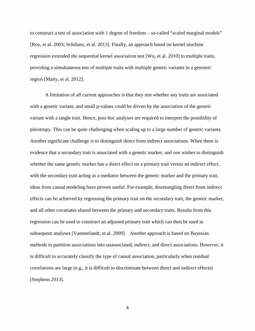
to construct a test of association with 1 degree of freedom – so-called “scaled marginal models”
[Roy, et al. 2003; Schifano, et al. 2013]. Finally, an approach based on kernel machine
regression extended the sequential kernel association test [Wu, et al. 2010] to multiple traits,
providing a simultaneous test of multiple traits with multiple genetic variants in a genomic
region [Maity, et al. 2012].
A limitation of all current approaches is that they test whether any traits are associated
with a genetic variant, and small p-values could be driven by the association of the genetic
variant with a single trait. Hence, post-hoc analyses are required to interpret the possibility of
pleiotropy. This can be quite challenging when scaling up to a large number of genetic variants.
Another significant challenge is to distinguish direct from indirect associations. When there is
evidence that a secondary trait is associated with a genetic marker, and one wishes to distinguish
whether the same genetic marker has a direct effect on a primary trait versus an indirect effect,
with the secondary trait acting as a mediator between the genetic marker and the primary trait,
ideas from causal modeling have proven useful. For example, disentangling direct from indirect
effects can be achieved by regressing the primary trait on the secondary trait, the genetic marker,
and all other covariates shared between the primary and secondary traits. Results from this
regression can be used to construct an adjusted primary trait which can then be used in
subsequent analyses [Vansteelandt, et al. 2009]. Another approach is based on Bayesian
methods to partition associations into unassociated, indirect, and direct associations. However, it
is difficult to accurately classify the type of causal association, particularly when residual
correlations are large (e.g., it is difficult to discriminate between direct and indirect effects)
[Stephens 2013].

7
The above methods are used to test whether a single genetic variant is associated with
multiple traits. When scaling up to genome-wide data, it has been useful to use all the genetic
markers to estimate the marker-predicted heritability of a trait. This has recently been extended
to multiple traits to estimate pleiotropy as the genetic correlation of multiple traits. Mixed
models are used to partition the phenotype correlations into genetic correlation (i.e., correlation
of polygenic total genetic values) and environmental correlation [Furlotte and Eskin 2015; Korte,
et al. 2012; Lee, et al. 2012; Zhou and Stephens 2014]. Although this approach does not evaluate
whether particular SNPs or particular genomic regions are the cause for phenotype correlations,
it has the potential to guide design of studies that focus on pleiotropy. For example, the
correlation of two phenotypes can be partitioned as 1 2 1 2P g er h h r e e r= + ,where 2ih is the heritability
of trait i, 2 21i ie h= − , gr is the genetic correlation, and er is the environmental correlation
[Falconer and Mackay 1996]( page 314). Heritability in the narrow sense is the percent of the
variance of the trait explained by additive genetic factors. This illustrates that if both traits have
low heritability, the phenotype correlation is primarily due to environmental correlation (and
non-additive genetic effects that are missed by gr ), implying that large sample sizes would be
needed to test pleiotropy when there are small genetic effects.
We have emphasized that current methods to evaluate pleiotropy do not perform a
formal test of the null hypothesis of no pleiotopy. For the special case of two traits, one can
construct a null hypothesis of no pleiotropy based on the intersection-union (IU) test [Silvapulle
and Sen 2004]. Consider the regression equation , 1,j o j j jy g eβ β= + + , where jy is the vector of
values for the thj trait, ,o jβ is the intercept, 1,iβ is the slope association parameter of interest, g is
the vector of doses for the minor allele, and je is a vector of residuals. The union null hypothesis

8
is 1,1 1,2: 0 or 0OH β β= = , and the intersection alternative hypothesis is 1 1,1 1,2: 0 and 0H β β≠ ≠ .
Testing each 1,iβ at a desired Type-I error, say 0.05α = , the null is rejected only if both tests
reject. There is no need to correct for multiple testing, because the Type-I error rate is not
inflated by this procedure. But, this approach can be conservative, particularly if the two tests are
uncorrelated. The IU test can be extended to 2p > traits, but rejection of the null would occur
only when all p tests are significant at the specified α . For our situation, we wish to reject the
null if at least two of the p tests reject. One approach would be to apply the IU test to each pair of
traits, and reject the null if at least one of the IU tests rejects. But, this would entail many pairs of
tests, and for this situation one would need to correct for testing multiple pairs. Bonferroni
correction would lead to an overly conservative test.
Because of current limitations, we developed a likelihood ratio test for testing the null
hypothesis of no pleiotropy – the null hypothesis that one or fewer traits are associated with a
genetic variant, versus the alternative hypothesis that two or more traits are associated. We then
extended the testing framework to test the null hypothesis that k or fewer traits are associated,
versus the alternative hypothesis that more than k traits are associated ( 0,1,... 1k p= − ). By this
generalization, we propose sequential testing to test the null hypothesis that 1k + traits are
associated, given that the null hypothesis of k traits are associated was rejected. This sequential
approach provides a refined approach to evaluate how many traits, and which traits, are
associated with a genetic variant, accounting for correlation among the traits, and possibly
adjusting for covariates that could differ across the traits.

9
Methods
Likelihood Ratio Test of Pleiotropy: Null of One or Fewer Traits
Suppose that p traits are measured on each of n subjects. Let 1( ,..., )j j jny y y′ = denote the
vector of measures on the thj trait for n subjects. Assume that each trait is modeled by linear
regression, denoted
= ,j j jy xβ ε+
where x is the dose of the minor allele for n subjects. Also assume that all jy and x are
centered, so intercepts can be ignored. For simplicity of presentation, we ignore adjusting
covariates, but our methods are general and allow for trait-specific covariates. By stacking
vectors, we can express the model as y Xβ ε= + , where 1( ,..., )py y y′ ′ ′= , ( )X diag x= ,
1( ,..., )pβ β β′ ′ ′= , and 1( ,..., )pε ε ε′ ′ ′= .The error term (0, )Nε Ω, where IΩ = Σ⊗ , I is an nxn
identify matrix, ⊗ is the Kronecker product, and the pxp matrix Σ is the covariance matrix for
the within-subject covariances of the errors. Under this model, the log-likelihood function of
( , )β Σ is given by
11( , ) = log | | ( ) ( )( ).2 2nnl y X I y Xβ β β−′Σ − Σ − − Σ ⊗ −
Suppose that the covariance Σ is known, otherwise, we can obtain a consistent estimate
by maximum likelihood estimation. For example, we we can estimate β by using methods from
seemingly unrelated regression, an approach called feasible generalized least squares. Separate
10
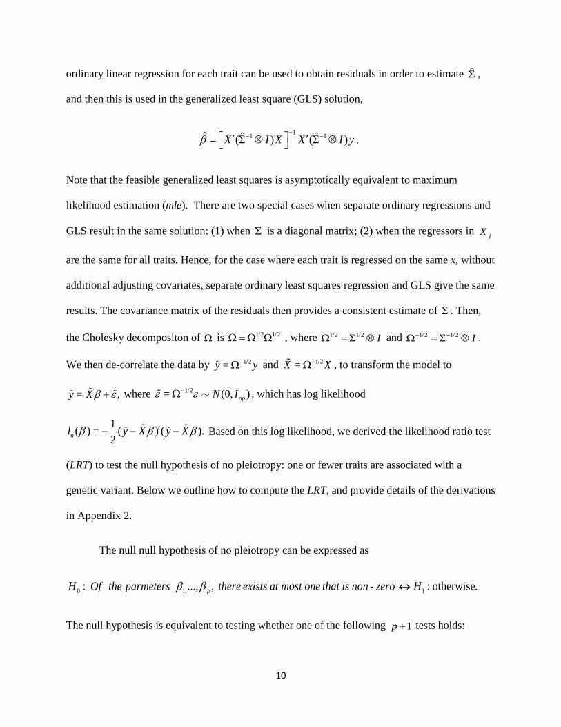
ordinary linear regression for each trait can be used to obtain residuals in order to estimate Σ ,
and then this is used in the generalized least square (GLS) solution,
11 1ˆ ˆ ˆ( ) ( )X I X X I yβ−− − ′ ′= Σ ⊗ Σ ⊗ .
Note that the feasible generalized least squares is asymptotically equivalent to maximum
likelihood estimation (mle). There are two special cases when separate ordinary regressions and
GLS result in the same solution: (1) when Σ is a diagonal matrix; (2) when the regressors in jX
are the same for all traits. Hence, for the case where each trait is regressed on the same x, without
additional adjusting covariates, separate ordinary least squares regression and GLS give the same
results. The covariance matrix of the residuals then provides a consistent estimate of Σ . Then,
the Cholesky decompositon of Ω is 1/2 1/2Ω = Ω Ω , where 1/2 1/2 IΩ = Σ ⊗ and 1/2 1/2 I− −Ω = Σ ⊗ .
We then de-correlate the data by 1/2=y y−Ω and 1/2=X X−Ω , to transform the model to
= ,y Xβ ε+
where 1/2= (0, )npN Iε ε−Ω , which has log likelihood
1( ) = ( ) ( ).2nl y X y Xβ β β′− − −
Based on this log likelihood, we derived the likelihood ratio test
(LRT) to test the null hypothesis of no pleiotropy: one or fewer traits are associated with a
genetic variant. Below we outline how to compute the LRT, and provide details of the derivations
in Appendix 2.
The null null hypothesis of no pleiotropy can be expressed as
0 1, 1: ..., , : otherwise.pH Of the parmeters there exists at most one that is non - zero Hβ β ↔
The null hypothesis is equivalent to testing whether one of the following 1p + tests holds:

11
0 : 0, = 0 ( )k k jH j kβ β≠ ≠ ,
for = 0, ,k p. Note that 00H represents all 0kβ = ( = 1, ,k p
), while for 0k > , 0kH allows
0kβ ≠ while all other 0 ( )j j kβ = ≠ . To represent these p+1 hypotheses, we use 0 : 0k kH V β = .
Let 0V be a matrix such that 00 0: 0H V β = tests whether all 0jβ = . This is the usual
multivariate test. In this case, 0V is the identity matrix of dimension p . To construct kV ( 0k > ),
create an identity matrix of dimension p , then remove the thk row. This results in
1 1 1( ,..., , )k k k pV β β β β β− + ′= .Then, the null hypothesis is equivalent to
0 0: : = 0, = 0, , .k kH there exists one of H V for k pβ
To construct the LRT, center y and x about their means, use ordinary least squares to estimate
,β use the residuals to estimate Σ , and then use Σ to decorrelate y and X according to
1/2 1/2= , =y y X X− −Ω Ω
, where 1/2 1/2 I− −Ω = Σ ⊗ . Then, for each = 0, ,k p, compute
1 1 1 1( ) [ ( ) ] ( )k k k k kt y X X X V V X X V V X X X y− − − −′ ′ ′ ′ ′ ′=
.
An alternative way to express kt is 2|| ||kk n Vt X Xβ β= − , the squared 2l norm between the fitted
values based on the ordinary least squares estimates, nβ , and the fitted values based on the
constrained esimates, kVβ (see Appendix 2).
As shown in Appendix 2, the LRT is
=0, ,= .min k
k pT t

12
Because jt is based on the sum of squared differences of the fitted values between the
unconstrained and constrained models, for a correctly specified contrained model, jt has a 2χ
distribution. But, the distribution of T is more complicated. The statisitc T has two different
asymptotic distributions depending on when β equals to zero or not. When = 0β , the
asymptotic distribution of each jt is a 2χ distribution, yet the distribution of the minimum of
them, T , is unknown. Alternatively, when = 0β , we can use the commonly used 2χ test for
the null hypothesis that all 0jβ = . This motivates us to do the test by two stages. The first stage
is just test 00H : = 0β , using the statistic 20 pt χ as the test statistic, so we reject 00H if
20 > ( )pt χ α , where 2 ( )pχ α is the 1 α− quantile of 2χ distribution with p degrees of freedom
(df). If 00H can not be rejected, then the 0H of no pleiotropy cannot be rejected. If 00H is
rejected, we turn to the second stage to test the null hypothesis that one 0kH holds for
= 1, , .k p For this we ignore 0t and use the test statisitc
1=1, ,
= .min kk p
T t
Since 21 1pT χ − , we reject the null hypothesis that only one 0kH holds for = 1, ,k p if
21 1> ( )pT χ α− . Then, the null hypthosis 0H of no pleiotropy is rejected only if both 00H is
rejected and null hypothesis that only one 0kH holds is rejected ( = 1, ,k p ).
To provide intuition why 1T has a large sample chi-square distribution with (p-1) df when
only one jβ differs from zero, while all others equal zero, we present an example in Figure 1. In
this example 1 0β ≠ and 0 ( 1)j jβ = ≠ . As shown in Appendix 2 (corollary 1), the distribution of

13
jt for a correctly specified model is 21pχ − . In contrast, the incorrect models result in arbitrarily
large values of jt (see corollary 2 of Appendix 2). This means that 1t will be minimum and
21 1~ pT t χ −= .
General Likelihood Ratio Sequential Testing: Null of K Associated Traits
The above sequential approach is based on testing the null hypothesis 00 : = 0H β ,
and then if this rejects, to turn to the second stage to test the null hypothesis that only one
0 : 0, 0 ( )k k jH j kβ β≠ = ≠ holds for = 1, ,k p . The advantage of this approach is that if 00H is
rejected and the null hypothesis that only one 0kH holds is accepted, one can conclude that there
is only one non-zero β . But, if the null hypothesis that only one 0kH holds is rejected , we
cannot make a firm conclusion aboult the number of traits associasted with a genetic variant. To
provide a more rigorous testing framework, we extended our approach to sequentially test the
null hypthothesis that a specified number of 'sβ are non-zero. So, if the null hypothesis that k
'sβ are non-zero is rejected, but the null hypothesis that 1k + 'sβ are non-zero is accepted,
we can conclude there are 1k + traits associated with a genetic variant. Futhermore, because the
sequential testing is based on a likelihood ratio framework, evaluating all possible combinations
of non-zero 'sβ , the combination that fails to reject the null hypothesis provides evidence of
which traits are assocaited with the genetic variant. The details of the statistical procedures of
this general sequential testing methods are provided in Appendix 2, as well as a proof that the
Type-I error is controlled. In summary, this general sequential procedure provides a formal way
to determine not only they number of traits associated with a genetic variant, but also which
traits are associated.

14
Simulations
To evaluate the adequacy of the 2χ distribution for the LRT, we performed simulations.
For the pleiotropy null, we performed two sets of simulations. The first assumed that all 0jβ = ,
the usual null for multivariate data. The second fixed 1 1β = and all other 0jβ = ( 2,...,j p= ).
The value of 1 1β = was chosen because the power for detecting this marginal effect size was
very large for our setup. We assumed three different sample sizes, 100, 500, 1000n = , and two
different values of 4, 10p = . The small sample size of 100n = was used to evaluate the
adequacy of our asymptotic derivations for small samples. The variance of the errors was
assumed to be 1, and the covariance was assumed to be either a constant ρ for all pairs of traits
(i.e., exchangeable correlation structure), or a range of covariances. For the range of covariances,
we randomly chose covariances from a specified range, assuming a uniform distribution of the
covariances. With a specified covariance structure, we simulated the random errors from either a
multivariate normal distribution or a multivariate t-distribution with 3 df, to evaluate the impact
of heavy-tailed distributions. For all simulations, a single SNP was simulated, assuming a minor
allele frequency of 0.2.
To evaluate the power of our proposed LRT for pleiotropy, we simulated 10 traits from a
multivariate normal distribution with variances of 1 and equal covariances among the traits, set
at 0.2, 0.5, or 0.8ρ = , for a total of n = 500 subjects. The number of traits associated with the
SNP ranged over 2, 3, or 5. The marginal effect of a trait was set at 0.25β = . This effect size
explains 2% of the variation of a trait, and there is 90% power to detect a marginal effect of this
size, using nominal 0.05α = . We also set the marginal effect to 0.2β = , which corresponds to an

15
explained 1.2% of the variation of a trait, and there is 70% power to detect a marginal effect of
this size. All simulations were repeated 1,000 times.
Data Application
Our newly developed LRT for pleiotropy was applied to a dataset that has 10 immunologic
phenotypes measured in response to primary smallpox vaccination. These phenotypes included
measures of humoral immunity (neutralizing antibody titer) and cellular immunity (two separate
IFNγ ELISPOT assays and cytokine secretion upon viral stimulation as measured by ELISA [IL-
1β, IL-2, IL-6, IL-12p40, IFNα, IFNγ, TNFα]) All 645 subjects included in the presented
analyses were of Caucasian ancestry. All subjects provided informed consent for use of their
samples and this study was approved by the Mayo Clinic Institutional Review Board. A genome-
wide association of the 10 phenotypes was performed, with each phenotype adjusted for relevant
covariates (i.e., p-value < .10 for association of a covariate with the phenotype, including
eigenvectors to adjust for potential population stratification). Details of the study can be found in
prior published reports [Kennedy, et al. 2012a; Kennedy, et al. 2012b; Ovsyannikova, et al.
2013; Ovsyannikova, et al. 2012a; Ovsyannikova, et al. 2012b; Ovsyannikova, et al. 2014].
Results
Simulation Results
The Type-I error rates based on simulations are presented in Tables 1-6. For all
simulations, we show results from the 2-stage test (using 0t for stage-1 and
1 min ; 1,..., kT t k p= = for stage-2), but in all cases, the results from the 2-stage test were

16
identical to the compound pleiotropy test = min ; 0,..., kT t k p= .The results for when only one
jβ differs from zero (Tables 1, 2, and 5) illustrate that the LRT can have inflated Type-I error
rates for small sample sizes ( 100n = ), with more extreme inflation as p increased from 4 to 10.
In contrast, for moderate to large sample sizes ( 500, 1000n = ), the Type-I error rates were
close to the nominal level, with only an occasional slight inflation. The inflated Type-I error rate
for small sample sizes seems to be caused by the need to estimate the covariance matrix of the
residuals. When we simulated errors that were independent, and used the identity matrix for the
residual correlations, the simulated Type-I error rates were very close to the nominal rates for all
sample sizes. In contrast, when all jβ were zero (Tables 3, 4, and 6), the LRT has conservative
Type-I error rates. This, however, is not of concern, because controlling the Type-I error rate
when only one jβ differs from zero is the major error that should be controlled when testing
pleiotropy. These results were consistent for different amounts and patterns of residual
correlations, and for multivariate normal and multivariate t distributions.
To further evaluate the adequacy of our asymptotic approximations for large samples, we
performed 10,000 simulations for 1,000 subjects and 4 traits that had a common correlation
structure. All but one β was zero; the non-zero β was chosen such that there was either 90% or
30% power to detect its marginal effect using 0.001α = . This scenario reflects modern large-
scale genomic studies that use more stringent significance thresholds. The quantile-quantile plots
in Figure 2 show that the asymptotic chi-square distribution to test pleiotropy provides adequate
p-values over the entire range of p-values for when the marginal effect of one β is small (power
of 30%) or large (power of 90%), and for when the correlation of the traits is small ( 0.2ρ = ) or
large ( 0.8ρ = ).
17
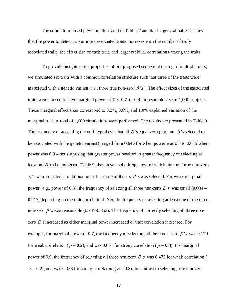
The simulation-based power is illustrated in Tables 7 and 8. The general patterns show
that the power to detect two or more associated traits increases with the number of truly
associated traits, the effect size of each trait, and larger residual correlations among the traits.
To provide insights to the properties of our proposed sequential testing of multiple traits,
we simulated six traits with a common correlation structure such that three of the traits were
associated with a genetic variant (i.e., three true non-zero ' sβ ). The effect sizes of the associated
traits were chosen to have marginal power of 0.3, 0.7, or 0.9 for a sample size of 1,000 subjects.
These marginal effect sizes correspond to 0.2%, 0.6%, and 1.0% explained variation of the
marginal trait. A total of 1,000 simulations were performed. The results are presented in Table 9.
The frequency of accepting the null hypothesis that all ' sβ equal zero (e.g., no ' sβ selected to
be associated with the genetic variant) ranged from 0.646 for when power was 0.3 to 0.015 when
power was 0.9 – not surprising that greater power resulted in greater frequency of selecting at
least one β to be non-zero . Table 9 also presents the frequency for which the three true non-zero
' sβ were selected, conditional on at least one of the six ' sβ was selected. For weak marginal
power (e.g., power of 0.3), the frequency of selecting all three non-zero ' sβ was small (0.034 –
0.213, depending on the trait correlation). Yet, the frequency of selecting at least one of the three
non-zero ' sβ was reasonable (0.747-0.862). The frequency of correctly selecting all three non-
zero ' sβ increased as either marginal power increased or trait correlation increased. For
example, for marginal power of 0.7, the frequency of selecting all three non-zero ' sβ was 0.179
for weak correlation ( ρ = 0.2), and was 0.851 for strong correlation ( ρ = 0.8). For marginal
power of 0.9, the frequency of selecting all three non-zero ' sβ was 0.472 for weak correlation (
ρ = 0.2), and was 0.956 for strong correlation ( ρ = 0.8). In contrast to selecting true non-zero

18
' sβ , we also present in Table 9 the frequency of wrongly selecting ' sβ that are truly zero. Not
surprisingly, when marginal power is weak (power of 0.3), if at least one β is selected, there is a
significant chance of wrongly selecting a true-zero β (e.g., frequency of 0.209 when ρ = 0.2).
This type of error decreased as the marginal power for traits increased and the trait correlation
increased. For example, when power was 0.9 and trait correlation was ρ = 0.8, the frequency of
selecting one true-zero β was 0.034, approaching the nominal Type-I error rate of 0.05. Table 9
illustrates that although there is a chance of wrongly selecting one true-zero β , the frequency of
selecting more than one true-zero β was small.
Data Application Results
Based on the traditional multivariate regression of all 10 traits on each SNP, we found a
strong association of at least one of the traits with SNPs in a region on chromosome 5 (see Figure
3). Figure 4 illustrates the traditional multivariate test 0( )t in a small region of chromosome 5
(left panel) and the LRT of pleiotropy in the same region (right panel). The test for pleiotropy
provides strong evidence that the signal of association was driven by a single phenotype. This is
confirmed qualitatively in Figure 5, which shows the individual marginal trait associations for
the chromosome 5 region. Although the individual marginal associations in Figure 5 give the
visual impression that only one trait is strongly associated with the chromosome 5 SNPs, the LRT
of pleiotropy provides a formal statistical test that accounts for the correlations among the traits.
19
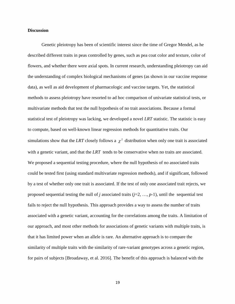
Discussion
Genetic pleiotropy has been of scientific interest since the time of Gregor Mendel, as he
described different traits in peas controlled by genes, such as pea coat color and texture, color of
flowers, and whether there were axial spots. In current research, understanding pleiotropy can aid
the understanding of complex biological mechanisms of genes (as shown in our vaccine response
data), as well as aid development of pharmacologic and vaccine targets. Yet, the statistical
methods to assess pleiotropy have resorted to ad hoc comparison of univariate statistical tests, or
multivariate methods that test the null hypothesis of no trait associations. Because a formal
statistical test of pleiotropy was lacking, we developed a novel LRT statistic. The statistic is easy
to compute, based on well-known linear regression methods for quantitative traits. Our
simulations show that the LRT closely follows a 2χ distribution when only one trait is associated
with a genetic variant, and that the LRT tends to be conservative when no traits are associated.
We proposed a sequential testing procedure, where the null hypothesis of no associated traits
could be tested first (using standard multivariate regression methods), and if significant, followed
by a test of whether only one trait is associated. If the test of only one associated trait rejects, we
proposed sequential testing the null of j associated traits (j=2, …, p-1), until the sequential test
fails to reject the null hypothesis. This approach provides a way to assess the number of traits
associated with a genetic variant, accounting for the correlations among the traits. A limitation of
our approach, and most other methods for associations of genetic variants with multiple traits, is
that it has limited power when an allele is rare. An alternative approach is to compare the
similarity of multiple traits with the similarity of rare-variant genotypes across a genetic region,
for pairs of subjects [Broadaway, et al. 2016]. The benefit of this approach is balanced with the

20
limitation of not knowing which genotypes are associated with which traits. Our proposed
sequential testing might provide a worthy follow-up procedure if some variants are not too rare.
Although our proposed methods assumed the subjects are independent, it is straight-
forward to extend our approach to pedigree data. To do so, the variance matrix of residuals for
independent subjects, ( ) ( )V Iε = Σ⊗ , would be replaced with ( ) ( )V Kε = Σ⊗ . The matrix K
contains diagonal elements 1 ii iK h= + where ih is the inbreeding coefficient for subject i, and
off-diagonal elements 2ij ijK j= . The parameter ijj is the kinship coefficient between
individuals i and j, the probability that a randomly chosen allele at a given locus from individual
i is identical by descent to a randomly chosen allele from individual j, conditional on their
ancestral relationship. For subjects from different pedigrees, 0ijj = , so K can be structured as a
block-diagonal matrix, with diagonal block iK for the thi pedigree. With this adjustment, our
methods can be used for pedigree data, or for data with population structure where matrix K is an
estimate of genetic relationships [Schaid, et al. 2013].
Application of our new approach to a study of immune phenotypes in response to
smallpox vaccination strongly suggests that only one of 10 correlated traits is statistically
associated with SNPs in a region on chromosome 5. The benefit of this type of analysis is that it
provides strong guidance on follow-up functional studies for genome-wide association studies
with multiple traits. In our case, it allowed investigators to focus on the single immunologic trait
truly associated with the chromosome 5 SNPs, rather than conducting labor-intensive, expensive,
and time-consuming experiments on unrelated immune response traits.
We recognize that our proposed LRT depends on the assumption that residuals have a
multivariate normal distribution. Our simulations with a multivariate t distribution (3 df) suggests

21
that the LRT is robust to heavy-tailed distributions. To assure robustness with the traditional
multivariate regression, it is common practice to transform the data to have at least normally
distributed marginal distributions, such as use of normal quantile transformation. This is a
reasonable approach for our proposed LRT.
A limitation of our method is that each of the traits is assumed to be quantitative. If all
traits are binary, or if there is a mixture of quantitative and binary traits, then the dependence of
the LRT on an assumed likelihood would need to be reconsidered. One approach is to consider
general multivariate exponential family of models [Prentice and Zhao 1991; Sammel, et al. 1997;
Zhao, et al. 1992]. Another approach would be to consider the reverse regression of a SNP dose
on all traits, like the ordinal logistic MultiPhen approach of [O'Reilly, et al. 2012], yet develop
an LRT for pleiotropy whereby one of the β ’s is allowed to be unconstrained under the null. An
alternative approach that we are developing is based on generalized linear models and
generalized estimating equations. The theoretical underpinnings of these alternate approaches,
and their computational challenges, are topics of future research.
Software for Pleiotropy
Software implementing the proposed tests for pleiotropy for quantitative traits is available as an
R package called “pleio” in the Comprehensive R Archive Network (https://cran.r-
project.org/web/packages/pleio/index.html).

22
Appendix 1.
R Code to compute F-statistic for canonical correlation of matrix Y with vector x.
library(CCA)
cc.fit <- cc(Y,x)
cc.fstat <- function(cc.fit)
rho <- cc.fit$cor
lambda <- 1 - rho^2
dimx <- max(dim(cc.fit$xcoef))
dimy <- max(dim(cc.fit$ycoef))
k <- max(c(dimx, dimy))
n <- nrow(Y)
fstat <- ((1-lambda)/lambda) * ((n-k-1)/k)
pval <- 1-pf(fstat, k, n-k-1, ncp=0)
return(list(fstat=fstat, pval=pval))
Appendix 2. Hypothesis Tests For Linear Model
Notation and Model
Based on the regression model described in the main text, suppose that p traits are
measured on each of n subjects, with 1( ,..., )j j jny y y′ = the vector of measures on the thj trait for n
subjects, and stack the vectors as 1( ,..., )py y y′ ′ ′= . Let ( )X diag x= , where x is a vector of length

23
n. We assume that y and x are centered on their means. We can express the model as
y Xβ ε= + , where 1( ,..., )pε ε ε′ ′ ′= .The error term (0, )Nε Ω, where IΩ = Σ⊗ and the pxp
matrix Σ is the covariance matrix for the within-subject covariances of the errors. Then, the
Cholesky decompositon of Ω is 1/2 1/2Ω = Ω Ω , where 1/2 1/2 IΩ = Σ ⊗ and 1/2 1/2 I− −Ω = Σ ⊗ .
Using 1/2 1/2= , =y y X X− −Ω Ω
, the model can transform to independent standard normal
random variables, = ,y Xβ ε+
where 1/2= (0, )npN Iε ε−Σ , and with log likelihood
1( ) = ( ) ( ).2nl y X y Xβ β β′− − −
Theorem 1. Let V be a k p× matrix of rank k ( )k p≤ . Then the minimizer of 2y Xβ−
under the constraint = 0Vβ is
*= ,V n Vβ β β−
where 1= ( )n X X X yβ −′ ′
is the ordinary least squares (OLS) estimate and
* 1 1 1 1= ( ) [ ( ) ] ( )V X X V V X X V V X X X yβ − − − −′ ′ ′ ′ ′ ′
.
Furthermore,
2 2 * 2= .V n Vy X y X Xβ β β− − +
(1)
Proof. Denote * = nβ β β− . Note that
2 2
2 * * *
2 * *
|| || || ( ) ||
|| || 2( )
|| || .
n n
n n
n
y X y X X
y X X X y X X
y X X X
β β β β
β β β β β
β β β
− = − + −
′ ′ ′= − + + −
′ ′= − +

24
The last above step results from *2( ) 0ny X Xβ β′− =
, because nyX X Xβ′ ′=
.
Under the constraint = 0Vβ , * = nV Vβ β . Applying the Lagrange multiplier method, we
minimize
* 2 * * *( , ) = 2 ( ).n nQ y X X X V Vβ λ β β β λ β β′− + + −
By taking the derivative of Q with respect to β and λ , we obtain the solution
* 1 1 1 1= ( ) [ ( ) ] ( )V X X V V X X V V X X X yβ − − − −′ ′ ′ ′ ′ ′
and the estimate of β is *=V n Vβ β β− .
Therefore, we have
2 2 * *|| = .V n V Vy X y X X Xβ β β β′ ′− − +
This completes the proof.
Remark: Equation (1) illustrates that the residual sums of squares (ssq) for the contrained model
( 2Vy Xβ−
) is partitioned into two parts: 1) the ssq for the OLS fit ( 2ny Xβ−
), and 2) the
sum of squared differences of the fitted values for the OLS model and the constrained model (
* 2 2|| ||V n VX X Xβ β β= −
).
Corrollary 1. Under the null Hypothesis: = 0Vβ ,
* 2 1 1 1 2 2= [ ( ) ] ( ) .V kX V X X V V X X Xβ ε χ− − −′ ′ ′ ′
Proof.

25
* 2 1 1 1 1 2
1 1 1 1
1 1 1 1
= ( ) [ ( ) ] ( )
( ) [ ( ) ] ( ) ( ) [ ( ) ] ( ) (
VX X X X V V X X V V X X X y
y X X X V V X X V V X X X XX X V V X X V V X X X y
y X X X
β − − − −
− − − −
− − − −
′ ′ ′ ′ ′ ′
′ ′ ′ ′ ′ ′ ′=
′ ′ ′ ′ ′ ′
′ ′=
1 1 1 1
1 1 1 1
) [ ( ) ] ( ) ( ) [ ( ) ] ( ) .
V V X X V V X X X yX X X V V X X V V X X Xε ε
− − − −
− − − −
′ ′ ′ ′ ′
′ ′ ′ ′ ′ ′ ′=
The substitution of y with ε in the last step of the above proof can be made because by the
assumed linear model, y X β ε= +
, we find that
1 1
1
1
( ) ( ) ( )( )
( )
V X X X y V X X X XV V X X XV X X X
β ε
β ε
ε
− −
−
−
′ ′ ′ ′= +
′ ′= +
′ ′=
The last step above results because 0Vβ = under the null hypothesis.
It is easy to verify that the matrix 1 1 1 1= ( ) [ ( ) ] ( )VP X X X V V X X V V X X X− − − −′ ′ ′ ′ ′ ′
is idempotent and is of rank k if the rank of V is of rank k . Because = (0, )npN Iε
and VP is
idempotent, 2V kPε ε χ′
, completing the proof.
Corrollary 2. If 0 0Vβ ≠ , then
* 2 = ( ) .VX O nβ →∞
Proof. It follows from the proof of Corrollary 1 that * 2 =V VX y P yβ ′
. By the linear model, we
have
*0 0 0= = 2V V V V VX y P y X P X P X Pβ β β ε ε β ε′ ′ ′ ′ ′ ′+ +

26
It is clear that 2 = (1)V k pP Oε ε χ′ and 1/2
0 = ( )V pX P O nβ ε′ ′ . In addition,
1 1 1 1 10 0 0 0= ( ) [ ( ) ] = ( ) [ ( ) ] = ( )VX P X V V X X V V n V V n X X V V O nβ β β β β β− − − − −′ ′ ′ ′ ′ ′ ′ ′ since
1 1 11 1( ) ( ) = (1)V n X X V V EX X V O− − −′′ ′ ′→ in probability. Combining all the three facts yields this
corrollary.
Hypothesis Tests
Now we consider the null hypothesis of no pleiotropy:
0 1, 1: ..., , : otherwise.pH Of the parmeters there exists at most one that is non - zero Hβ β ↔
The null hypothesis is equivalent to testing whether one of the following 1p + tests holds:
0 : 0, 0 ( )k k jH j kβ β≠ = ≠ ,
for = 0, ,k p. Note that 00H represents all 0kβ = ( = 1, ,k p
), while for 0k > , 0kH allows
0kβ ≠ while all other 0 ( )j j kβ = ≠ .
To represent these 1p + hypotheses, we use 0 : 0k kH V β = . Let 0V be a matrix such that
00 0: 0H V β = tests whether all 0jβ = . In this case, 0V is the identity matrix of dimension p . To
construct kV ( 0k > ), create an identity matrix of dimension p , then remove the thk row. This
results in 1 1 1( ,..., , )k k k pV β β β β β− + ′= .Then, the null hypothesis is equivalent to
0 0: : = 0, = 0, , .k kH there exists one of H V for k pβ
For = 0,1, ,k p , set =k Vkt y P y′ . Then it follows from Theorem 1 that

27
2 2= || ,k V nkt X Xβ β−
where Vkβ is the least squares estimate under the constraint = 0kV β and
1 1 1 1= ( ) [ ( ) ] ( ) .V k k k kkP X X X V V X X V V X X X− − − −′ ′ ′ ′ ′ ′
Then we have the following corollary.
Corollary 3. The likelihood ratio test (LRT), 2− times log of ratio of likelihoods, is
given by
=0, ,
= .min kk p
T t
If 00H holds, then
= ,k Vkt Pε ε′
and 2 20 1, p k pt tχ χ − for = 1, ,k p .
If only one 0kH ( > 0)k holds, then
21.pT χ −
From Corollary 3, one can see that the test statisitc T has two different asymptotic distributions
when β equals to zero or not. When = 0β , the asymptotic distribution of T is unknown.
Alternatively, when = 0β , we can use the commonly used 2pχ test for the null hypothesis that
all 0jβ = . This motivates us to do the test by two stages. The first stage is just test 00H : = 0β ,
using the statistic 20 pt χ as the test statistic, so we reject 00H if 2
0 > ( )pt χ α , where 2 ( )pχ α is

28
the 1 α− quantile of 2χ distribution with p degrees of freedom. If 00H can not be rejected, then
0H cannot be rejected. If 00H is rejected, we turn to the second stage to test the null hypothesis
that one 0kH holds for = 1, ,k p . Then we can use the test statistic 1=1, ,
= .min kk p
T t
Since 21 1pT χ −
, we reject the null hypothesis that one 0kH holds for = 1, ,k p if 21 1> ( )pT χ α− . Then, the null
hypthosis 0H is rejected only if both 00H is rejected and null hypothesis that one 0kH holds is
rejected ( = 1, ,k p ). Since both tests are conducted at Type-I error rate of α , and this is based
on the principal of the intersection-union (IU) test [Silvapulle and Sen 2004], the Type-I error
rate for rejecting 0H is no more than α .
Remark. If p is too large, it might be beneficial to ignore the 0t and directly use 21 1pT χ − to
construct the rejection region.
Sequential Test of Nonzero Beta’s
The above solutions can be easily extended to test the following null hypothesis:
0 1: : .H There exists at most K nonzero components of H otherwiseβ↔
With appropriately defined V matrices (there are pKC matrices), the LRT reduces to
2
=1, ,= ,min Vkpk CK
T P y
where 1 1 1 1= ( ) [ ( ) ] ( ) .V k k k kkP X X X V V X X V V X X X− − − −′ ′ ′ ′ ′ ′

29
In the above, kV is a ( )p K p− × matrix. For example, if for indices 11 < < Ki i p≤ ≤ ,
we test
110, , 0 = 0, , , ,i i j KK
and j i iβ β β≠ ≠ ≠
then we can constitute the corresponding matrix , ,1i iKV
as follows: (i) constitute a p p× identity
matrix; (ii) delete the rows for indices 1, , Ki i .
Then we can use the following multi-stage test.
i. First test 00H : = 0β . Reject if 20 > ( )pt χ α . If reject, go onto the next stage,
otherwise stop and conclude 00H is true.
ii. For = 1, , 1s K − , test 0 :sH there are only s components of β unequal to zero.
Reject 0sH if 2> ( )s p sT χ α− , where , ,1 < < 11
= .mins Vi ii i p ss
T y P y≤ ≤
′
The indices range over
the psC choices. If reject, continue testing by incrementing s by 1. If fail to reject
0sH , stop testing and conclude there are s traits associated with x.
The Type-I error rate of this sequential testing is no greater than the nominal α level. To
understand this, suppose there are K non-zero β ’s, and define the Type-I error as concluding
there are K> non-zero β ’s. Note that the test statistic sT at each stage is based on the minimum
of statistics, where each statistic is based on * 2 2|| ||V n VX X Xβ β β= −
, a measure of distance
between fitted values based on the unconstrained OLS model and the constrained model
determined by V. If one of the constrained models is correct, then by corollarries 1 and 2,

30
2~sT χ . If, however, none of the constrained models are correct, = ( )sT O n →∞ . This means
that at testing stage j K< , the probability of rejecting the null hypothesis at stage j depends on
the power to detect the misspecified models, which approach 1 as n increases. With this
background, we can formally evalaute the Type-I error rate. Define jr as an indicator of whether
the null hypothesis is rejected at stage j. The probability of a Type-I error is the probability of
rejecting the sequential stage testing up to and including stage K. This joint probability can be
expressed a
0 1 2 0 1 0 2 0 1 0 1 1( , , ,..., ) ( ) ( | ) ( | , )... ( | , ,..., )K K KP r r r r P r P r r P r r r P r r r r −= (2)
The last term in expression (2) represents the probability of rejecting the null hypothesis when
the null hypothesis is true, so one of the constrained models is correct. The test statisic at stage
K follows a 2p Kχ − distribution, so 0 1 1( | , ,..., )K KP r r r r α− = . All other terms in (2) approach 1 as n
increases, because all stages j K< represent misspecified models. This proves that Type-I error
rate is no greater than the specified α level.
Acknowledgements
This research was supported by 1) the U.S. Public Health Service, National Institutes of Health,
contract grant number GM065450 (DJS) ; 2) federal funds from the National Institute of
Allergies and Infectious Diseases, National Institutes of Health, Department of Health and
Human Services, under Contract No. HHSN266200400025C (N01AI40065) (GAP); and 3) the
National Natural Science Foundation of China (Grant No. 11371062), Beijing Center for
Mathematics and Information Interdisciplinary Sciences, China Zhongdian Project (Grant No.

31
11131002) (XT). The content is solely the responsibility of the authors and does not necessarily
represent the official views of the National Institutes of Health.
Dr. Poland is the chair of a Safety Evaluation Committee for novel investigational
vaccine trials being conducted by Merck Research Laboratories. Dr. Poland offers consultative
advice on vaccine development to Merck & Co. Inc., CSL Biotherapies, Avianax, Dynavax,
Novartis Vaccines and Therapeutics, Emergent Biosolutions, Adjuvance, and Microdermis. Dr.
Poland holds two patents related to vaccinia and measles peptide research. Dr. Kennedy has
grant funding from Merck Research Laboratories to study immune responses to mumps vaccine.
These activities have been reviewed by the Mayo Clinic Conflict of Interest Review Board and
are conducted in compliance with Mayo Clinic Conflict of Interest policies. This research has
been reviewed by the Mayo Clinic Conflict of Interest Review Board and was conducted in
compliance with Mayo Clinic Conflict of Interest policies.

32
References
Berkson J. 1946. Limitations of the application of fourfold table analysis to hospital data. Biometrics Bulletin 2(3):47-53.
Broadaway KA, Cutler DJ, Duncan R, Moore JL, Ware EB, Jhun MA, Bielak LF, Zhao W, Smith JA, Peyser PA and others. 2016. A Statistical Approach for Testing Cross-Phenotype Effects of Rare Variants. American journal of human genetics 98(3):525-40.
Cotsapas C, Voight BF, Rossin E, Lage K, Neale BM, Wallace C, Abecasis GR, Barrett JC, Behrens T, Cho J and others. 2011. Pervasive sharing of genetic effects in autoimmune disease. PLoS genetics 7(8):e1002254.
Denny JC, Bastarache L, Ritchie MD, Carroll RJ, Zink R, Mosley JD, Field JR, Pulley JM, Ramirez AH, Bowton E and others. 2013. Systematic comparison of phenome-wide association study of electronic medical record data and genome-wide association study data. Nature biotechnology 31(12):1102-10.
Falconer D, Mackay T. 1996. Introduction to Quantitative Genetics. New York: Pearson Prentice Hall. Ferreira MA, Purcell SM. 2009. A multivariate test of association. Bioinformatics 25(1):132-3. Furlotte N, Eskin E. 2015. Efficient multiple-trait association and estimation of genetic correaltion using
the matrix-variate linear mixed model. Genetics 200:59-68. Galesloot TE, van Steen K, Kiemeney LA, Janss LL, Vermeulen SH. 2014. A comparison of multivariate
genome-wide association methods. PloS one 9(4):e95923. Gianola D, de los Campos G, Toro M, H N, Schon C, Sorensen D. 2015. Do molecular markers inform
about pleiotropy? Genetics Early online. Kennedy RB, Ovsyannikova IG, Pankratz VS, Haralambieva IH, Vierkant RA, Jacobson RM, Poland GA.
2012a. Genome-wide genetic associations with IFNgamma response to smallpox vaccine. Human genetics 131(9):1433-51.
Kennedy RB, Ovsyannikova IG, Pankratz VS, Haralambieva IH, Vierkant RA, Poland GA. 2012b. Genome-wide analysis of polymorphisms associated with cytokine responses in smallpox vaccine recipients. Human genetics 131(9):1403-21.
Korte A, Vilhjalmsson BJ, Segura V, Platt A, Long Q, Nordborg M. 2012. A mixed-model approach for genome-wide association studies of correlated traits in structured populations. Nature genetics 44(9):1066-71.
Lee S, Yang J, Goddard M, Visscher P, Wray N. 2012. Estimation of pleiotropy between complex diseases using single-nucleotide polymorphism-derived genomic relationships and restricted maximum likelihood. Bioinformatics 28:254-2542.
Liu J, Pei Y, Papasian CJ, Deng HW. 2009. Bivariate association analyses for the mixture of continuous and binary traits with the use of extended generalized estimating equations. Genetic epidemiology 33(3):217-27.
Maier R, Moser G, Chen GB, Ripke S, Coryell W, Potash JB, Scheftner WA, Shi J, Weissman MM, Hultman CM and others. 2015. Joint analysis of psychiatric disorders increases accuracy of risk prediction for schizophrenia, bipolar disorder, and major depressive disorder. American journal of human genetics 96(2):283-94.
Maity A, Sullivan PF, Tzeng JY. 2012. Multivariate phenotype association analysis by marker-set kernel machine regression. Genetic epidemiology 36(7):686-95.
Marchini J, Howie B, Myers S, McVean G, Donnelly P. 2007. A new multipoint method for genome-wide association studies by imputation of genotypes. Nat Genet 39(7):906-13.
O'Reilly PF, Hoggart CJ, Pomyen Y, Calboli FC, Elliott P, Jarvelin MR, Coin LJ. 2012. MultiPhen: joint model of multiple phenotypes can increase discovery in GWAS. PloS one 7(5):e34861.

33
Ovsyannikova IG, Haralambieva IH, Kennedy RB, O'Byrne MM, Pankratz VS, Poland GA. 2013. Genetic variation in IL18R1 and IL18 genes and Inteferon gamma ELISPOT response to smallpox vaccination: an unexpected relationship. The Journal of infectious diseases 208(9):1422-30.
Ovsyannikova IG, Haralambieva IH, Kennedy RB, Pankratz VS, Vierkant RA, Jacobson RM, Poland GA. 2012a. Impact of cytokine and cytokine receptor gene polymorphisms on cellular immunity after smallpox vaccination. Gene 510(1):59-65.
Ovsyannikova IG, Kennedy RB, O'Byrne M, Jacobson RM, Pankratz VS, Poland GA. 2012b. Genome-wide association study of antibody response to smallpox vaccine. Vaccine 30(28):4182-9.
Ovsyannikova IG, Pankratz VS, Salk HM, Kennedy RB, Poland GA. 2014. HLA alleles associated with the adaptive immune response to smallpox vaccine: a replication study. Human genetics 133(9):1083-92.
Prentice RL, Zhao LP. 1991. Estimating equations for parameters in means and covariances of multivariate discrete and continuous responses. Biometrics 47:825-839.
Roy J, Lin X, Ryan LM. 2003. Scaled marginal models for multiple continuous outcomes. Biostatistics 4(3):371-83.
Sammel M, Ryan L, Legler J. 1997. Latent variable models for mixed discrete and continuous outcomes. J Royal Statist Soc, Series B 59(3):667-678.
Schaid DJ, McDonnell SK, Sinnwell JP, Thibodeau SN. 2013. Multiple genetic variant association testing by collapsing and kernel methods with pedigree or population structured data. Genetic epidemiology 37(5):409-18.
Schifano ED, Li L, Christiani DC, Lin X. 2013. Genome-wide association analysis for multiple continuous secondary phenotypes. American journal of human genetics 92(5):744-59.
Schriner D. 2012. Moving toward system genetics through multiple trait analysis in genome-wide association studies. Frontiers in Genetics 16(7):1-7.
Silvapulle MJ, Sen PK. 2004. Constrained Statistical Inference: Order, Inequality, and Shape Constraints. New York: John Wiley and Sons, Inc.
Solovieff N, Cotsapas C, Lee PH, Purcell SM, Smoller JW. 2013. Pleiotropy in complex traits: challenges and strategies. Nature reviews. Genetics 14(7):483-95.
Stephens M. 2013. A unified framework for association analysis with multiple related phenotypes. PloS one 8(7):e65245.
Vansteelandt S, Goetgeluk S, Lutz S, Waldman I, Lyon H, Schadt EE, Weiss ST, Lange C. 2009. On the adjustment for covariates in genetic association analysis: a novel, simple principle to infer direct causal effects. Genetic epidemiology 33(5):394-405.
Wu MC, Kraft P, Epstein MP, Taylor DM, Chanock SJ, Hunter DJ, Lin X. 2010. Powerful SNP-set analysis for case-control genome-wide association studies. Am J Hum Genet 86(6):929-42.
Xu Z, Pan W. 2015. Approximate score-based testing with application to multivariate trait association analysis. Genetic epidemiology 39(6):469-79.
Yang Q, Wang Y. 2012. Methods for Analyzing Multivariate Phenotypes in Genetic Association Studies. Journal of probability and statistics 2012:652569.
Zhang Y, Xu Z, Shen X, Pan W. 2014. Testing for association with multiple traits in generalized estimation equations, with application to neuroimaging data. NeuroImage 96:309-25.
Zhao LP, Prentice RL, Self SG. 1992. Multivariate mean parameter estimation by using a partly exponential model. J R Statist Soc B 54(3):805-811.
Zhou X, Stephens M. 2014. Efficient multivariate linear mixed model algorithms for genome-wide association studies. Nature methods 11(4):407-9.

34
Table 1. Empirical Type-I error rate for common correlation structure when 1 1β = and
all other 0jβ = ( 1j ≠ ), based on multivariate normal distribution. Underlined values
for when empirical Type-I error exceeds upper 95% CI interval.
Sample
Size No.
Traits Trait
Correlation Nominal Type-I
Error Rate 0.05 0.01
100 4 0.2 0.072 0.020 0.5 0.070 0.016 0.8 0.066 0.014 10 0.2 0.105 0.036 0.5 0.092 0.032 0.8 0.094 0.029
500 4 0.2 0.056 0.017 0.5 0.058 0.011 0.8 0.058 0.009 10 0.2 0.061 0.010 0.5 0.056 0.011 0.8 0.068 0.019
1000 4 0.2 0.052 0.012 0.5 0.058 0.008 0.8 0.051 0.010 10 0.2 0.057 0.012 0.5 0.052 0.010 0.8 0.046 0.007

35
Table 2. Empirical Type-I error rate for random correlation structure when 1 1β = and all
other 0jβ = ( 1j ≠ ), based on multivariate normal distribution. Underlined values for
when empirical Type-I error exceeds upper 95% CI interval.
Sample Size
No. Traits
Trait Correlation
Nominal Type-I
Error Rate 0.05 0.01
100 4 0-0.2 0.066 0.011 0.2-0.5 0.065 0.013 0.5-0.8 0.055 0.011 10 0-0.2 0.077 0.018 0.2-0.5 0.106 0.029 0.5-0.8 0.112 0.039
500 4 0-0.2 0.065 0.007 0.2-0.5 0.049 0.015 0.5-0.8 0.047 0.008 10 0-0.2 0.049 0.011 0.2-0.5 0.067 0.016 0.5-0.8 0.053 0.012
1000 4 0-0.2 0.042 0.007 0.2-0.5 0.055 0.009 0.5-0.8 0.043 0.009 10 0-0.2 0.072 0.012 0.2-0.5 0.056 0.012 0.5-0.8 0.056 0.011

36
Table 3. Empirical Type-I error rate for common correlation structure when all 0jβ = ,
based on multivariate normal distribution.
Sample Size
No. Traits
Trait Correlation
Nominal Type-I Error Rate
0.05 0.01 100 4 0.2 0.005 0.002
0.5 0.006 0.001 0.8 0.009 0.002 10 0.2 0.015 0 0.5 0.011 0 0.8 0.014 0.003
500 4 0.2 0.003 0 0.5 0.005 0.001 0.8 0.011 0.001 10 0.2 0.005 0.001 0.5 0.003 0.001 0.8 0.009 0.001
1000 4 0.2 0.005 0 0.5 0.008 0 0.8 0.004 0.001 10 0.2 0.011 0.002 0.5 0.012 0 0.8 0.009 0.002

37
Table 4. Empirical Type-I error rate for random correlation structure when all 0jβ = ,
based on multivariate normal distribution.
Sample Size
No. Traits
Trait Correlation
Nominal Type-I Error Rate
0.05 0.01 100 4 0-0.2 0.005 0
0.2-0.5 0.012 0.001 0.5-0.8 0.014 0.001 10 0-0.2 0.018 0.002 0.2-0.5 0.01 0.002 0.5-0.8 0.029 0.004
500 4 0-0.2 0.004 0 0.2-0.5 0.009 0 0.5-0.8 0.007 0.001 10 0-0.2 0.009 0 0.2-0.5 0.009 0.001 0.5-0.8 0.019 0.005
1000 4 0-0.2 0.006 0.001 0.2-0.5 0.006 0 0.5-0.8 0.004 0 10 0-0.2 0.01 0.002 0.2-0.5 0.01 0 0.5-0.8 0.01 0

38
Table 5. Empirical Type-I error rate when 1 1β = and all other 0jβ = ( 1j ≠ ), based on
multivariate t- distribution with 3 df, with common correlation structure. Underlined values for when empirical Type-I error exceeds upper 95% CI interval.
Sample Size
No. Traits
Trait Correlation
Nominal Type-I Error Rate
0.05 0.01 100 4 0.2 0.042 0.011
0.5 0.067 0.019 0.8 0.057 0.015 10 0.2 0.088 0.018 0.5 0.104 0.028 0.8 0.094 0.030
500 4 0.2 0.059 0.011 0.5 0.038 0.007 0.8 0.043 0.009 10 0.2 0.041 0.016 0.5 0.059 0.021 0.8 0.050 0.010
1000 4 0.2 0.052 0.006 0.5 0.047 0.006 0.8 0.054 0.009 10 0.2 0.054 0.010 0.5 0.058 0.015 0.8 0.055 0.016

39
Table 6. Empirical Type-I error rate when all 0jβ = , based on multivariate t-
distribution with 3 df, with common correlation structure.
Sample Size
No. Traits
Trait Correlation
Nominal Type-I Error Rate
0.05 0.01 100 4 0.2 0.009 0
0.5 0.007 0 0.8 0.011 0.002 10 0.2 0.015 0.001 0.5 0.015 0.002 0.8 0.013 0.003
500 4 0.2 0.003 0 0.5 0.005 0 0.8 0.005 0 10 0.2 0.009 0.001 0.5 0.008 0 0.8 0.008 0.001
1000 4 0.2 0.004 0.001 0.5 0.009 0.001 0.8 0.007 0.001 10 0.2 0.011 0.001 0.5 0.002 0 0.8 0.011 0.001

40
Table 7. Power to detect pleiotropy when associated traits have 0.25β = (explain 2%
trait variation; power = 90% for marginal effect). Multivariate normal distribution with equal correlation structure, for sample size of 500 subjects and minor allele frequency of genetic variant set to 0.20.
No. Associated Traits ( 0.25β = )
Trait Correlation
Nominal Type-I Error Rate
0.05 0.01 2 0.2 0.503 0.237
0.5 0.801 0.581
0.8 0.971 0.900 3 0.2 0.859 0.677
0.5 0.956 0.858
0.8 0.999 0.998 5 0.2 0.980 0.928
0.5 0.999 0.985
0.8 1.000 1.000

41
Table 8. Power to detect pleiotropy when associated traits have 0.2β = (explain 1.2%
trait variation; power = 70% for marginal effect). Multivariate normal distribution with equal correlation structure, for sample size of 500 subjects and minor allele frequency of genetic variant set to 0.20.
No. Associated Traits ( 0.2β = )
Trait Correlation
Nominal Type-I Error Rate
0.05 0.01 2 0.2 0.220 0.069
0.5 0.393 0.165
0.8 0.964 0.850 3 0.2 0.494 0.255
0.5 0.715 0.478
0.8 1.000 0.991 5 0.2 0.842 0.636
0.5 0.907 0.750
0.8 1.000 1.000

42
Table 9. Properties of sequential testing for 6 traits: proportions out of 1,000 simulations with no β ’s selected, proportions according to the number of true non-zero β ’s selected, and proportions according to the number of zero β ’s falsely selected. Marginal power is for detecting the effect of a single trait in a sample size of 1,000 subjects ( 0.05α = ), and the corresponding β and trait explained variation are provided.
Marginal Power
β
Explained Variation
(%) Trait Corr.
No β ’s Selected Number True β ’s Selected
0 1 2 3 0.3 0.081 0.2 0.2 0.646 0.138 0.644 0.184 0.034
0.5 0.830 0.235 0.471 0.229 0.065 0.8 0.850 0.253 0.267 0.267 0.213
0.7 0.139 0.6 0.2 0.128 0.048 0.361 0.412 0.179 0.5 0.169 0.113 0.178 0.337 0.372 0.8 0.169 0.105 0.011 0.034 0.851
0.9 0.180 1.0 0.2 0.014 0.007 0.109 0.413 0.472 0.5 0.015 0.030 0.028 0.172 0.770 0.8 0.015 0.043 0.001 0.000 0.956
Number β ’s Falsely Selected
0 1 2 3
0.3 0.081 0.2 0.2
0.782 0.209 0.008 0.000 0.5
0.694 0.247 0.053 0.006
0.8
0.693 0.127 0.140 0.040 0.7 0.139 0.6 0.2
0.867 0.119 0.011 0.002
0.5
0.792 0.140 0.057 0.012 0.8
0.864 0.024 0.019 0.093
0.9 0.180 1.0 0.2
0.923 0.071 0.005 0.001 0.5
0.920 0.048 0.017 0.015
0.8
0.918 0.034 0.005 0.044

43
Figure Legends
Figure 1. Example to illustrate why the pleiotropy LRT has an approximate 21pχ − distribution
when only one jβ differs from zero. For this example, 1 0β ≠ and 0 ( )j j iβ = ≠ . Then, 1t will be
the minimum because it measures the sum of squared differences of the fitted values for the
unconstrained ordinary least squares model and the constrained model, which in this case is
correctly specified. Because all other ( 1)jt j ≠ represent mis-specified models, their values can
become arbitrarily large as n increases. Hence, the correctly specified model will have the
smallest values of jt . And, the distribution of jt for a correctly specified model is 21pχ − .
Figure 2. Quantile-quantile plots of p-values to test the null hypothesis of no pleiotropy. Sample
size was 1,000 with 4 equally correlated traits ( 0.2 or 0.8ρ = ). All but one β was zero; the non-
zero β was chosen such that there was either 30% or 90% power to detect its marginal effect
using 0.001α = . A total of 10,000 simulations were performed.
Figure 3. Manhattan plot of the multivariate regression of 10 traits on each SNP, using statistic
0t , to test whether any of the traits are associated with a SNP. The red horizontal line
corresponds to a p-value of 85 10−× , and the blue line for a p-value of 510− .

44
Figure 4. Zoomed-in region of chromosome 5, comparing the traditional multivariate regression
of 10 traits on each SNP (left panel) with the pleiotropy LRT for the same traits and region.
Figure 5. Zoomed-in region of chromosome 5 for each of the univariate regression results for the
10 traits. Trait-5 is the only trait showing strong associations with SNPs on region of
chromosome 5.

*
1( ,0,...,0)
1t
jt
pt
*(0,0,..., ,...,0)j *(0,0,..., )p

0 1 2 3 4
01
23
4
Expected − log10(p)
Obs
erve
d −
log 1
0(p
)marginal power =.9, ρ = 0.2
0 1 2 3 4
01
23
45
Expected − log10(p)
Obs
erve
d −
log 1
0(p
)
marginal power =.9, ρ = 0.8
0 1 2 3 4
01
23
4
Expected − log10(p)
Obs
erve
d −
log 1
0(p
)
marginal power =.3, ρ = 0.2
0 1 2 3 4
01
23
Expected − log10(p)
Obs
erve
d −
log 1
0(p
)marginal power =.3, ρ = 0.8

Chromosome
1 2 3 4 5 6 7 8 9 10 11 12 13 14 15 16 17 18 21 22 X 19 20
0
5
10
1
5
-log1
0(p
-val
ue)

0 50 100 150 200 250
05
1015
20
position
−lo
g10(
p−va
lue)
Multivariate Test
0 50 100 150 200 250
05
1015
20
position
−lo
g10(
p−va
lue)
Pleiotropy Test

0 100 200
position
−lo
g10(
pval
)
Trait−10
510
15
0 100 200
position
−lo
g10(
pval
)
Trait−2
05
1015
0 100 200
position
−lo
g10(
pval
)
Trait−3
05
1015
0 100 200
position
−lo
g10(
pval
)
Trait−4
05
1015
0 100 200
position
−lo
g10(
pval
)
Trait−5
05
1015
0 100 200
position
−lo
g10(
pval
)
Trait−6
05
1015
0 100 200
position
−lo
g10(
pval
)
Trait−7
05
1015
0 100 200
position
−lo
g10(
pval
)
Trait−8
05
1015
0 100 200
position
−lo
g10(
pval
)
Trait−9
05
1015
0 100 200
position
−lo
g10(
pval
)
Trait−10
05
1015