1

Statistical method for risk management and portfolio

theory

A Major Qualifying Project

Submitted to the Faculty of the

WORCESTER POLYTECHNIC INSITUTE

in partial fulfillment of the requirements for the degree of Bachelor of Science

Submitted by:

_______________

Zhenyan Li

Mathematical Science. Class of 2016

December 10, 2015

_______________________

Advisor: Professor Jian Zou

This report represents work of WPI undergraduate students submitted to the faculty as evidence of a degree requirement. WPI routinely publishes these reports on its web site without editorial or peer review. For

more information about the projects program at WPI, see http://www.wpi.edu/Academics/Projects.

2

Abstract

The portfolio theory is a risk management framework through the concept of

diversification. When investing, the theory attempts to maximize portfolio expected return

or minimize portfolio risk for a given level of expected return by choosing the proportions

of various assets. The project focuses on the Dow 30 companies’ activity in 2014 and

generalizes the return of the 30 assets to find the one with the highest return. Based on the

regression analysis, we found two assets with maximum return and minimum risks. We

ran the model diagnostics on the regression model and removed the outliers to reduce the

bias. To find the best portfolio, we combined these two assets into the tangency portfolio

and added a risk-free asset (Treasury Yield Curve Rate) into the portfolio. To evaluate the

performance of the combined portfolio, we applied risk measures including Value-at Risk,

the Sharpe ratio and the Sortino ratio as well as formulated the most desirable portfolio in

terms of reward-to-risk criteria for investment. This project was accomplished by

combining the applications of multiple linear regression analysis, model diagnostics and

portfolio theory. The implementation was achieved by statistical language R and EXCEL.

Key words: Regression analysis; Risk Management; Portfolio Theory; Expected Return

3

Acknowledgements

Without the help from certain individuals, the completion of this project would not

have been possible. First, I would like to thank my advisor, Professor Zou, for giving me

the opportunity to work with him and providing me with the topic as well as for his

guidance, support and patience during the summer and the last three terms. I must finally

thank my academic advisor, Professor Blais, for his valuable advice.

4

Table of Contents

1 Introduction and Background ..............................................................................8

1.1 Introduction ..............................................................................................................8

1.2 Literature Reviews .................................................................................................10

2 Methodology .........................................................................................................15

Overview ................................................................................................................15

2.1 Returns ...................................................................................................................16

2.1.1 Net Return ..................................................................................................16

2.1.2 Log Returns ................................................................................................16

2.2 Regression ..............................................................................................................17

2.2.1 Straight-line Regression .............................................................................17

2.2.2 Multiple Linear Regression .......................................................................18

2.3 Portfolio Theory .....................................................................................................18

2.3.1 One Risky Asset and One Risk-Free Asset................................................19

2.3.2 Two Risky Assets ......................................................................................19

2.3.3 Combining Two Risky Assets with a Risk-Free Asset ..............................19

2.3.4 Risk measurement for Portfolio performance ............................................21

3 Results ...................................................................................................................23

3.1 Security Valuation .................................................................................................24

3.1.1 Generalizing Security.................................................................................24

3.1.2 Finding two Risky Assets ..........................................................................26

3.1.3 Model Diagnostics .....................................................................................30

5

3.2 Asset Allocation .....................................................................................................33

3.2.1 Transferring the Risk-free Rate .................................................................33

3.2.2 Tangency Portfolio.....................................................................................34

3.3 Portfolio Optimization ...........................................................................................35

3.3.1 Targeting a Certain Expected Return .........................................................36

3.3.2 Targeting Certain Volatility .......................................................................36

3.4 Performance Measurement ....................................................................................39

3.4.1 Value-at-Risk .............................................................................................39

3.4.2 Sharpe Ratio ...............................................................................................39

3.4.3 Sortino Ratio ..............................................................................................40

3.5 INTC with KO .......................................................................................................42

4 Conclusion ............................................................................................................47

4.1 Results summary ....................................................................................................47

4.2 Future Work ...........................................................................................................48

Appendix A .......................................................................................................................49

R codes ..........................................................................................................................49

Appendix B .......................................................................................................................52

Excel Forms ..................................................................................................................52

Annualized Return and risk ...........................................................................................52

Downside Deviation output ...........................................................................................52

Performance Measurement of portfolios .......................................................................52

Plot INTC~KO without outliers ...................................................................................52

6

List of Tables

Table 1: Sheet of Return and Risk of Dow 30 (2015.01-2015.09) ...................................24

Table 2: Sheet of Return and Risk of Dow 30 sort by return (2014.01-2014.12) ............25

Table 3: Sheet of Return and Risk of Dow 30 sort by risk (2014.01-2014.12) ................26

Table 4: Sheet of Correlation .............................................................................................27

Table 5: Update Return and Risk of 2 risky assets ............................................................32

Table 6: Return and Risk sheet of two Risky Assets and Risk-free Asset ........................33

Table 7: Daily Return and Risk sheet ................................................................................33

Table 8: Tangency Portfolio weight ..................................................................................34

Table 9: Daily Tangency Portfolio output .........................................................................35

Table 10: Annualized return and risk output .....................................................................35

Table 11: Combined Portfolio Outputs ..............................................................................37

Table 12: VaR of portfolio .................................................................................................39

Table 13: Sharpe ratio outputs ...........................................................................................40

Table 14: Sortino ratio outputs ..........................................................................................41

Table 15: The overall performance measurement .............................................................42

Table 16: Return and Risk sheet (INTC&KO) .................................................................44

Table 17: Tangency portfolio outputs (INTC&KO) .........................................................45

Table 18: Annualized return and risk outputs (INTC&KO) .............................................45

Table 19: Performance measurement output .....................................................................45

7

List of Figures

Figure 1: R call output of model1 ......................................................................................28

Figure 2: multiple linear regressions (R codes) ................................................................30

Figure 3: Diagnostics in R: Plot (model) ..........................................................................31

Figure 4: Diagnostics in R: plot (model.2) .......................................................................32

Figure 5: Portfolio plots (R) ..............................................................................................38

Figure 6: Diagnostics in R (INTC~ KO) ..........................................................................43

Figure 7: Plot INTC~KO without outliers .......................................................................44

8

Chapter 1

Introduction and Background

1.1 Introduction

Statistics is widely defined as the study of the collection, classification, analysis

and interpretation of data (Dodge, 2003). People can apply statistics as a tool to find

trends in large amounts of data to predict the performance of such data. Furthermore,

Statistics plays an important role in a number of different fields including math,

economics, business, financing, investing, industry, engineering, accounting, biology and

social science. Business managers apply statistics to perform the market research, find the

customer preferences, estimate costs and profits in order to make decisions. Economists

use statistics to find the relationship between supply and demand, the imports and exports,

the inflation rate and estimate the trend of the market. Accountants carry out statistics to

evaluate the performance, discover the profit trends, build the financial statement and

setup the revenue goal for next season. Investors apply statistics to combine various assets

and find the proportion of the assets to ensure more return with lower risk. The examples

show how people are using statistical methods to analyze data to reasonably invest and

manage assets and the broader social and economical impacts of statistics. The project

will focus on the application of statistics in financing and investing with an emphasis on

the risk management.

Risk Management is a rich subject which includes many aspects such as assets

9

allocation, security valuation, portfolio optimization and performance measurement. In

this project, we focus on the statistical methods for controlling the risk and portfolio

allocation. Risk is always uncertain and it is related to certainty quantification. It is the

threat when an event could impede the companies’ or the market’s current development

by affecting the firm’s ability to achieve its business goal successfully. Risk accompanies

all kinds of business activities, thus, it is an inherent components and sometimes

unavoidable. The objective of risk management is not to completely prevent or eliminate

all risks. It is about making decisions in order to efficiently manage and respond to the

risks by maximizing the benefits and minimizing the adverse effects.

Regression is a statistical tool used to understand and estimate the relationship

between two or more variables. The primary application of regression in business and

finance is forecasting. For example, the investors rely on regression analysis to estimate

the relationship between the asset activities and interest rate. The companies’ advertising

department applies regression analysis to estimate the relation between corporation’s sales

and advertising expenditures. Also, the regression can be used to forecast the future

demand for a product in a company.

Performance measurement is the process of collecting, analyzing and reporting of

the information to help us understand, manage, and improve our goal. It usually tells us

how well we are doing, if there is space to improve, if we are meeting our goals, if our

customers are satisfied, etc. There are multiple approaches of performance measurements

such as return on investment, number of accidents per day, units of mile per gallon, etc.

These units or numbers tell people about the efficiency, productivity, safety, quality, etc.

Performance measure is widely used in many industries in real life and it is one of the

10

most significant topics we will talk in our project since we need these measurements to

reflect the profitability of our portfolio.

In the project, we downloaded 30 Dow Jones companies’ activities in 2014 and

generated the return & risk list to find the asset with the highest expected return. We used

regression analysis to find two assets with maximum return and minimum risks. We used

the portfolio theory to combine these two assets into the tangency portfolio and added a

risk-free asset into the portfolio to find a better one. To evaluate the performance of the

combined portfolio, we used Value-at Risk, the Sharpe ratio and the Sortino ratio. The

ultimate goal of the project is to combine the tangency portfolio with the risk-free asset

and to achieve the lowest overall risk with the highest expected return in terms of the

reward-to-risk criteria. This project is mostly accomplished with the application of

regression analysis and portfolio theory.

We will introduce the formulas and definitions in our application in the

Methodology Chapter which have a great amount of studies and development behind

them.

1.2 Literature Reviews

The study of risk can be traced to Markowitz’s work on Portfolio Theory which

stated that investors should care about risks as well as return, since the future is not

known as certainty but variations of this type of rule can be suggested (1952). After that,

the science of risk management has developed and became its own study of field. Risk

management is defined to be the identification, assessment, and prioritization of risks.

Risk management is a two-step process: firstly determine the risks existing in the

11

investment, and then deal with the risk to minimize it in the investment. Risk management

a subject combining both the statistical analysis and financial skills to identify and

effectively response to the emerging risks. The companies rely on risk managers to ensure

that no unforeseeable events would negatively impact the company. Risk managers

analyze data and learn lessons from risk events as well as obtain the unbiased and

independent data from the source to evaluate and respond to the risks. According to

Ruppert (2011):

There are many different types of risk. Market risk is due to changes in

prices. Credit risk is the danger that counterparty does not meet

contractual obligation, for example, that interest or principal on a bond

is not paid. Liquidity risk is the potential extra cost of liquidating a

position because buyers are difficult to locate. Operational risk is due to

fraud, mismanagement, human errors, and similar problems.

Miller developed a framework for categorizing the uncertainties faced by firms operating

internationally and proposed both financial and strategic corporate risk management

responses (1992). Slovic brought up methods for assessing perceptions of risk and the

implications for regulation and public policy in his book (2000). He examined the gap

between expert views of risk and public perceptions. The risk management as an

enterprise-wide approach is really important in an organization. If a company defines its

objective without taking the risks into account, they will definitely lack the methods on

how to respond once the risks emerge. That is why risk management is especially critical

for people who work in the business area.

The regression model is the most important method in data analysis. Hundreds of

12

years ago, the original form of regression was the method of least squares published by

Legendre in 1805 and Gauss in 1809. Gauss published a further theory of least squares in

1821. The term “regression” was firstly coined by Francis Galton in the 19th century, and

the original meaning described a biological phenomenon (return to a former stage). But

it’s meaning had been extended to a more general statistical context which shows

relationship between the selected values of predictor x and observed values of response y

(Yule, 1897 & Karl & Yule, 1903). Regression analysis has its unique application in the

real life. Marketing department applies the regression to forecast the future demand and

investors carry out it to optimize the benefits. In our project, regression models were

performed to estimate the relationship between the assets activities and to optimize the

expected return.

The Portfolio Theory is another significant topic we will introduce and apply in

the project. It was first introduced in the book “Portfolio Selection” (Harry M. Markowitz,

1952). Markowitz proposed an “expected returns-variance of returns” rule and won the

Nobel memorial prize for the theory in 1990. The theory is widely used in the financial

industry. The modern portfolio theory explains how to select a portfolio with the highest

possible expected return on a given level of risk, or for a given expected return, how to

select a portfolio with the lowest possible risk (Edwin & Gruber, 1997). The Capital Asset

Pricing Model (CAPM) was introduced by several people, who referred to the earlier

work of Markowitz on portfolio theory (Frencha, 2003). This model describes the

relationship between risk and expected return. Arbitrage pricing theory (APT) proposed

by Stephen Ross (1976) is another theory of asset pricing that states that the return of a

financial asset can be predicted using the relationship between the asset and many

13

common risk factors. APT is often viewed as an alternative to the CAPM. The difference

is that APT has multiple factors whereas CAPM has a single factor. Moreover, APT

considers various macro-economic factors and has more assumption requirements than

CAPM. The Fama-French Three-factor model is another model introduced by Eugene

Fama and Kenneth French (1993) to describe stock returns with three variables instead of

one variable used by the capital pricing model. In our project, we apply portfolio theory to

find the allocating distribution of our two risky assets and one risk-free asset in order to

combine our desirable portfolio with maximized return and minimized risk.

The Sharpe ratio, arguably the most common way to measure the financial

performance of an investment, was developed in 1966 by William F. Sharpe, and used to

be called the “reward-to-variability” ratio by Sharpe. In 1983, the Sortino ratio, a further

development of Sharpe ratio, was created by Brian M. Rom but it was named after Frank

A. Sortino who popularized downside risk optimization. Different from the Sharpe ratio,

the Sortino ratio only penalizes the standard deviation of negative return asset. Thus the

Sortino ratio is better at analyzing portfolios with high volatility than the Sharpe ratio

(Sortino, 2010). The Sharpe ratio and the Sortino ratio are the most significant two

measurements in our project and reflect the efficiency of our portfolios. Another measure

of performance analysis, value-at-risk (VaR), did not emerge as a distinct concept until

the late 1980s because of the stock market crash in 1987. The market crash prompted the

risk managers to think about the new measure model to predict the actual risk

emergement. The approach to model selection for predicting VaR, consisting of

alternative risk models and comparing strategies for choosing VaR models, was proposed

in 2009 (McAleer, Jimenez-Martin, Perez-Amaral). VaR measures the predictable

14

financial risk on an investment portfolio over a specific time and it is used to estimate the

actual risk and compare the portfolios with the initial assets.

15

Chapter 2

Methodology

Overview

First of all, we chose the Dow Jones 30 companies as our targeted assets. We downloaded

the daily historical price of the Dow 30 companies and the daily one-year Treasury Yield

Curve Rate. We got the daily returns for each asset using the log return and copied them

into a new sheet. Then, we calculate the expected return (the average log return) and the

volatility (the standard deviation of the log returns), for each asset and sort expected

return from largest to smallest. We picked up the asset with the largest return as our

Asset1 and used the multiple regressions model to find the least correlated asset to Asset1

as our Asset2. We used R language to apply the multiple regressions model. During the

procedure, we also used residual diagnostics for regression to determine the validation of

the model assumption and remove the outliers. After finding our two targeted assets, we

began to allocate the assets and optimize the portfolio. We firstly found the weight for the

two assets in the tangency portfolio and then combined the tangency portfolio with the

risk-free asset. To find out the final proportion of the tangency portfolio and risk-free

asset, we set up our targeted return and volatility first. After we found the combined

portfolios, we also evaluated the portfolio performance by some reward-to-risk measures.

To better understand the procedure of this project, the following subsections introduce the

formulations and definitions we used in the project. The interested readers can find the

following formulation from e.g., Ruppert, 2011.

16

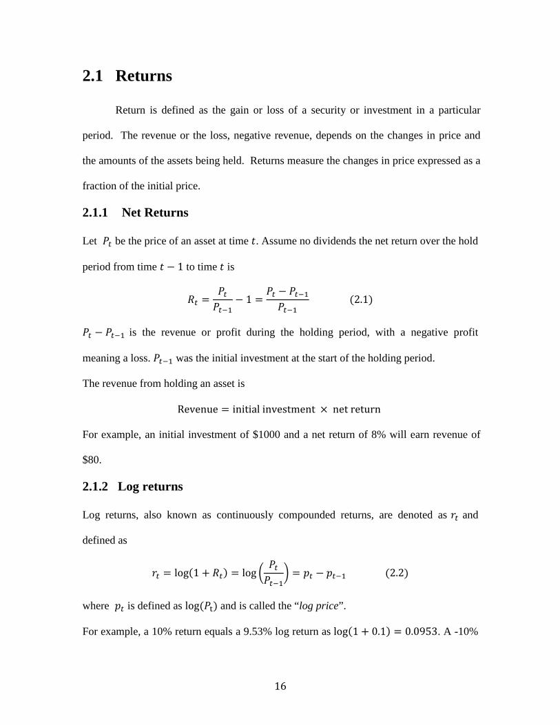
2.1 Returns

Return is defined as the gain or loss of a security or investment in a particular

period. The revenue or the loss, negative revenue, depends on the changes in price and

the amounts of the assets being held. Returns measure the changes in price expressed as a

fraction of the initial price. 2.1.1 Net Returns

Let 𝑃𝑃𝑡𝑡 be the price of an asset at time 𝑡𝑡. Assume no dividends the net return over the hold

period from time 𝑡𝑡 − 1 to time 𝑡𝑡 is

𝑅𝑅𝑡𝑡 =𝑃𝑃𝑡𝑡𝑃𝑃𝑡𝑡−1

− 1 =𝑃𝑃𝑡𝑡 − 𝑃𝑃𝑡𝑡−1𝑃𝑃𝑡𝑡−1

(2.1)

𝑃𝑃𝑡𝑡 − 𝑃𝑃𝑡𝑡−1 is the revenue or profit during the holding period, with a negative profit

meaning a loss. 𝑃𝑃𝑡𝑡−1 was the initial investment at the start of the holding period.

The revenue from holding an asset is

Revenue = initial investment × net return

For example, an initial investment of $1000 and a net return of 8% will earn revenue of

$80.

2.1.2 Log returns

Log returns, also known as continuously compounded returns, are denoted as 𝑟𝑟𝑡𝑡 and

defined as

𝑟𝑟𝑡𝑡 = log(1 + 𝑅𝑅𝑡𝑡) = log �𝑃𝑃𝑡𝑡𝑃𝑃𝑡𝑡−1

� = 𝑝𝑝𝑡𝑡 − 𝑝𝑝𝑡𝑡−1 (2.2)

where 𝑝𝑝𝑡𝑡 is defined as log(𝑃𝑃t) and is called the “log price”.

For example, a 10% return equals a 9.53% log return as log(1 + 0.1) = 0.0953. A -10%

17

return equals a -10.54% log return since log(1 − 0.1) = −0.1054. Also, log(1 +

0.05) = 0.0488 and log(1 − 0.05) = −0.0513.

Log return is significant here in the project, we use (2.2) to get the log return of each 2

days prices and calculate the mean of these continuous log returns, which is the expected

return.

2.2 Regression

Let 𝑌𝑌 be the response variable and 𝑋𝑋1, … ,𝑋𝑋𝑝𝑝 be the predictor variables. 𝑌𝑌𝑖𝑖 and

𝑋𝑋𝑖𝑖,1, … ,𝑋𝑋𝑖𝑖,𝑝𝑝 are the values of these variables for the ith observation. The regression

modeling investigates how Y is related to 𝑋𝑋1, … ,𝑋𝑋𝑝𝑝, estimates the conditional expectation

of Y given 𝑋𝑋1, … ,𝑋𝑋𝑝𝑝, and prediction of future Y values when the corresponding values of

𝑋𝑋1, … ,𝑋𝑋𝑝𝑝 are already available.

The multiple linear regression model rating Y to the predictor variables is

𝑌𝑌𝑖𝑖 = 𝛽𝛽0 + 𝛽𝛽1𝑋𝑋𝑖𝑖,1 + ⋯+ 𝛽𝛽𝑝𝑝𝑋𝑋𝑖𝑖,𝑝𝑝 + 𝜖𝜖𝑖𝑖

where 𝜖𝜖𝑖𝑖 is the random noise. 𝛽𝛽0 is the intercept, it is the expected value of 𝑌𝑌𝑖𝑖 when all

the 𝑋𝑋𝑖𝑖,𝑗𝑗 are zero. The coefficients of 𝛽𝛽1, … ,𝛽𝛽𝑝𝑝 are the corresponding slopes of

𝑋𝑋𝑖𝑖,1, … ,𝑋𝑋𝑖𝑖,𝑝𝑝. 𝛽𝛽𝑗𝑗 Indicates every unit change in the expected value of 𝑌𝑌𝑖𝑖 when 𝑋𝑋𝑖𝑖,𝑗𝑗 changes

on unit.

2.2.1 Straight-Line Regression

Straight-line regression is linear regression with only one predictor variable. The model

is

𝑌𝑌𝑖𝑖 = 𝛽𝛽0 + 𝛽𝛽1𝑋𝑋𝑖𝑖 + 𝜖𝜖𝑖𝑖 (2.3)

18

where 𝛽𝛽0 and 𝛽𝛽1 are the intercept and slope of the line.

2.2.2 Multiple Linear Regression

The multiple linear regression model is

𝑌𝑌𝑖𝑖 = 𝛽𝛽0 + 𝛽𝛽1𝑋𝑋𝑖𝑖,1 + ⋯+ 𝛽𝛽𝑝𝑝𝑋𝑋𝑖𝑖,𝑝𝑝 + 𝜖𝜖𝑖𝑖 (2.4)

We use the multiple linear regression model in R to find out the pair of assets with the

smallest correlation. We firstly test the asset with the largest return with the other 29

assets and take into account the most correlated one, and test this new asset with the rest

28 assets and so forth. In the end, the last asset left is the least correlated to the first asset.

2.3 Portfolio Theory

Portfolio theory, also known as modern portfolio theory (MPT) or portfolio management

theory, is a theory based on how the investors construct the portfolios to optimize the

expected return on a given level of risk.

There are four steps:

• Security valuation

• Asset allocation

• Portfolio optimization

• Performance measurement

We will see the details of the four steps in the Results Chapter when we carry out the real

data analysis.

19

2.3.1 One Risky Asset and One Risk-Free Asset

Assume the expected return and standard deviation of a risky asset is 𝜇𝜇 and 𝜎𝜎, and there

is also on risk-free asset with return of 𝜇𝜇𝑓𝑓 and standard deviation 𝜎𝜎𝑓𝑓 = 𝑜𝑜. Suppose that a

fraction w of our wealth is invested in the risky asset and the remaining fraction 1 − 𝑤𝑤 is

invested in the risk-free asset. Then the expected return is

𝐸𝐸(𝑅𝑅) = 𝑤𝑤𝜇𝜇 + (1 − 𝑤𝑤)𝜇𝜇𝑓𝑓 (2.5)

The variance of the return is

𝜎𝜎𝑅𝑅2 = 𝑤𝑤2𝜎𝜎2 + (1 − 𝑤𝑤)2(0)2 = 𝑤𝑤2𝜎𝜎2

and the standard deviation of the return is

𝜎𝜎𝑅𝑅 = 𝜎𝜎𝑤𝑤 (2.6)

2.3.2 Two Risky Assets

Suppose two risky assets have returns 𝑅𝑅1 and 𝑅𝑅2 and we mix them in proportion w and

1 − 𝑤𝑤 . The return is 𝑅𝑅 = 𝑤𝑤𝑅𝑅1 + (1 − 𝑤𝑤)𝑅𝑅2. The expected return on the portfolio is

𝐸𝐸(𝑅𝑅) = 𝑤𝑤𝜇𝜇1 + (1 − 𝑤𝑤)𝜇𝜇2 . Let 𝜌𝜌12 be the correlation between the returns on the two

risky assets. The variance of the return on the portfolio is

𝜎𝜎𝑅𝑅2 = 𝑤𝑤2𝜎𝜎12 + (1 − 𝑤𝑤)2𝜎𝜎22 + 2𝑤𝑤(1 − 𝑤𝑤)𝜌𝜌12𝜎𝜎1𝜎𝜎2 (2.7)

Note that 𝜎𝜎𝑅𝑅1,𝑅𝑅2 = 𝜌𝜌12𝜎𝜎1𝜎𝜎2.

2.3.3 Combining Two Risky Assets with a Risk-Free Asset

Tangency Portfolio with Two Risky Assets

Again, let 𝜇𝜇1, 𝜇𝜇2 and 𝜇𝜇𝑓𝑓 be the expected returns on the two risky assets and the

return on the risk-free asset. Let 𝜎𝜎1 and 𝜎𝜎2 be the standard deviations of the returns

on the two risky assets and let 𝜌𝜌12 be the correlation between the returns on the

20

risky assets.

Define 𝑉𝑉1 = 𝜇𝜇1 − 𝜇𝜇𝑓𝑓 and 𝑉𝑉2 = 𝜇𝜇2 − 𝜇𝜇𝑓𝑓, the excess expected returns. Then the

tangency portfolio uses weight

𝑤𝑤𝑇𝑇 =𝑉𝑉1𝜎𝜎22 − 𝑉𝑉2𝜌𝜌12𝜎𝜎1𝜎𝜎2

𝑉𝑉1𝜎𝜎22 + 𝑉𝑉2𝜎𝜎12 − (𝑉𝑉1 + 𝑉𝑉2)𝜌𝜌12𝜎𝜎1𝜎𝜎2 (2.8)

For the first risky asset and weight (1 − 𝑤𝑤𝑇𝑇) for the second.

Let 𝑅𝑅𝑇𝑇 ,𝐸𝐸(𝑅𝑅𝑇𝑇), and 𝜎𝜎𝑇𝑇 be the return, expected return, and standard deviation of the

return on the tangency portfolio. Then 𝐸𝐸(𝑅𝑅𝑇𝑇) and 𝜎𝜎𝑇𝑇 can be found by first finding 𝑤𝑤𝑇𝑇

using (2.8) and using the formulas

𝐸𝐸(𝑅𝑅𝑇𝑇) = 𝑤𝑤𝑇𝑇𝜇𝜇1 + (1 − 𝑤𝑤𝑇𝑇)𝜇𝜇2 (2.9)

and

𝜎𝜎𝑇𝑇 = �𝑤𝑤𝑇𝑇2𝜎𝜎12 + (1 − 𝑤𝑤𝑇𝑇)2𝜎𝜎22 + 2𝑤𝑤𝑇𝑇(1 − 𝑤𝑤𝑇𝑇)𝜌𝜌12𝜎𝜎1𝜎𝜎2 (2.10)

These formulas above are crucial to our project, since we use them to find the

weight 𝑤𝑤𝑇𝑇 for our tangency portfolio.

Combining the Tangency Portfolio with the Risk-free Asset

Let 𝑅𝑅𝑝𝑝 be the return on the portfolio that allocates a fraction 𝜔𝜔 of the investment to the

tangency portfolio and 1 − 𝜔𝜔 to the risk-free asset. Then

𝑅𝑅𝑝𝑝 = 𝜔𝜔𝑅𝑅𝑇𝑇 + (1 − 𝜔𝜔)𝜇𝜇𝑓𝑓 = 𝜇𝜇𝑓𝑓 + 𝜔𝜔(𝑅𝑅𝑇𝑇 − 𝑅𝑅𝑓𝑓)

so that

𝐸𝐸(𝑅𝑅𝑃𝑃) = 𝜇𝜇𝑓𝑓 + 𝜔𝜔{𝐸𝐸(𝑅𝑅𝑇𝑇) − 𝜇𝜇𝑓𝑓} and 𝜎𝜎𝑅𝑅𝑃𝑃 = 𝜔𝜔𝜎𝜎𝑇𝑇 . (2.11)

After finding the tangency portfolio in our project, we use (2.11) find the combing weight

𝜔𝜔.

21

2.3.4 Risk measurement for Portfolio performance

VaR

In financial risk management, value-at-risk is a risk measure of the level of financial risk

on a investment portfolio over a specific time. The risk managers always use it to estimate

and control the level of risk which the firm could undertake.

Suppose a portfolio of investment has a one-month 5% VaR of $1 million, this means that

there is 5% chance that the portfolio will fall in value of more than $1 million in any

given month.

Sharpe ratio

Sharpe ratio is a way to measure the performance of investment by calculating risk-

adjusted return. The Sharpe ratio measures the excess return per unit of volatility or risk

(standard deviation) in an investment asset.

𝑆𝑆ℎ𝑎𝑎𝑟𝑟𝑝𝑝𝑎𝑎 𝑟𝑟𝑎𝑎𝑡𝑡𝑟𝑟𝑜𝑜 =𝐸𝐸(𝑅𝑅𝑃𝑃) − 𝜇𝜇𝑓𝑓

𝜎𝜎𝑅𝑅𝑃𝑃

Sharpe ratio is last but significant part in our project since measurement of performance

plays an important role in the risk management project. A larger Sharpe ratio means a

higher expected return for a given level of risk, thus, the larger Sharpe ratio, the better the

portfolio is performing.

Sortino ratio

Sortino ratio is a modification of Sharpe ratio that differentiates the harmful volatility by

focusing on the standard deviation of the negative asset returns which is downside

deviation, different from Sharpe ratio penalizes both upside and downside volatility. A

large sortino ratio indicates the probability of a large loss is low.

22

𝑠𝑠𝑜𝑜𝑟𝑟𝑡𝑡𝑟𝑟𝑠𝑠𝑜𝑜 𝑟𝑟𝑎𝑎𝑡𝑡𝑟𝑟𝑜𝑜 = 𝐸𝐸(𝑅𝑅𝑃𝑃) − 𝜇𝜇𝑓𝑓

𝜎𝜎𝑑𝑑 (2.13)

where 𝜎𝜎𝑑𝑑 = Standard deviation of negative asset returns.

Sortino ratio is better than Sharpe ratio when analyzing a portfolio with high volatility.

Effect of 𝝆𝝆𝟏𝟏𝟏𝟏

According to (2.10), the smaller 𝜌𝜌12, the smaller the risk is. Thus, positive correlation

between two risky assets is not good since it will increase the volatility. Conversely,

negative correlation is good. When 𝜌𝜌12 is small, the efficient portfolio has less risk for a

given level of return compare to a larger 𝜌𝜌12. This is significant in our project, since our

goal is to maximize the return and minimize the risk. Thus, we have to find a pair of two

assets with the correlation between them as small as possible to minimize the risk based

on the given level of return.

23

Chapter 3

Results

First of all, we chose the Dow Jones 30 companies as our targeted assets. We downloaded

the daily historical price of the Dow 30 companies and the daily Treasury Yield Curve

Rate from January 2015 to September 2015. We got the daily return for each asset using

the Formula 2.2 and copied them into a new sheet. Then, we calculated the expected

return (the average of the 166 data) and the volatility (the standard deviation of the return)

for each asset and sorted the Expected Return column by largest to smallest. The list is

shown in Table 1 below.

Company Expected Return Volatility NKE 0.00036246 0.005427245 UNH 0.000308778 0.006704323 HD 0.000272074 0.005618419 DIS 0.000170144 0.006447469 V 0.000117591 0.0059978 MCD 7.36645E-05 0.005132488 PFE 6.70026E-05 0.00475848 BA -1.53483E-06 0.005932228 AAPL -5.7528E-06 0.007468806 JPM -9.47463E-06 0.006003824 VZ -5.68783E-05 0.004250472 GE -7.96061E-05 0.006028705 GS -0.000144628 0.005647444 TRV -0.000174514 0.004829707 KO -0.000175244 0.003783511 MRK -0.000180369 0.005854845 CSCO -0.000205998 0.006410425 MSFT -0.000237981 0.007895184 IBM -0.000271929 0.005707904

24

JNJ -0.000272409 0.004535395 3M -0.000389884 0.00471668 CAT -0.000464768 0.006417421 AXP -0.000568849 0.006167833 XOM -0.000592784 0.005871294 UTX -0.000601334 0.005339694 INTC -0.00063737 0.00696479 PG -0.00064696 0.004331788 WMT -0.000723041 0.005000283 DD -0.000822185 0.006342017 CVX -0.000864191 0.007036405 Risk-free rate 0.002643976 0.000572549

Table 1: Sheet of Return and Risk of Dow 30 (2015.01-2015.09)

However, the largest return among the 30 companies of NKE (Nike, Inc.) is still smaller

than the average daily Treasury Yield Rate. In this case, we cannot continue with the

negative excess expected returns (the difference between return of risky asset and risk-

free asset), since this means the risk-free asset leads to a higher return than the risky asset,

which is a meaningless portfolio construction. The low expected return is caused by the

bad performance of the stock happening in 2015, as the overall market is experiencing a

sharp decline during 2015.

To avoid negative excess expected return, we selected a time period with a better

market performance. Accordingly, we decided to analyze the assets performance in 2014

when the overall market performed better than 2015.

3.1 Security Valuation

3.1.1 Generalizing Assets

After making the final decision on the time period, we downloaded all Dow 30

companies’ historical daily prices from January 2014 to December 2014 and measured the

25

log returns by the Formula 2.2 between each two-day prices. We had 251 expected returns

for each asset, then we calculated the expected return and standard deviation of the 251

data and combined them into a new excel sheet. After sorting these data by expected

return from largest to smallest, we got that INTC (Intel Corporation) is the security with

the highest expected return. The result is shown in Table 2 below.

Company Expected Return Volatility INTC 0.000644984 0.006016181 AAPL 0.000614366 0.005924446 UNH 0.000554677 0.005131256 HD 0.000463851 0.004542265 CSCO 0.000447134 0.004572712 MSFT 0.000432838 0.005201736 DIS 0.000386997 0.004849593 NKE 0.000377597 0.005720839 MMM 0.00034187 0.004118795 TRV 0.000333134 0.003234185 V 0.000308706 0.005774122 DD 0.000305251 0.004369133 MRK 0.000290118 0.005215922 JNJ 0.00028725 0.003990711 PG 0.00026678 0.003195245 WMT 0.000189261 0.003637665 GS 0.000180835 0.004747392 JPM 0.000159794 0.004896901 KO 0.00011624 0.004112382 PFE 9.8599E-05 0.004406175 AXP 8.68251E-05 0.004876352 CAT 7.71345E-05 0.004972695 UTX 7.50764E-05 0.004166835 MCD 9.33574E-06 0.003458593 VZ -4.56371E-06 0.00405599 BA -4.69131E-05 0.005286244 XOM -8.31201E-05 0.004522835 GE -8.62938E-05 0.004121864 CVX -0.00011466 0.004972695 IBM -0.000209891 0.004729747

Table 2: Sheet of Return and Risk of Dow 30 sort by return (2014.01-2014.12)

26

There is another way to evaluate these 30 assets by looking at the risk level. If we

sort these data by volatility from smallest to largest, we can conclude that PG (The

Procter & Gamble Company) is the least risky asset among 30 assets. We attach the list in

Table 3 below.

Company Expected Return Volatility PG 0.00026678 0.003195245 TRV 0.000333134 0.003234185 MCD 9.33574E-06 0.003458593 WMT 0.000189261 0.003637665 JNJ 0.00028725 0.003990711 VZ -4.56371E-06 0.00405599 KO 0.00011624 0.004112382 MMM 0.00034187 0.004118795 GE -8.62938E-05 0.004121864 UTX 7.50764E-05 0.004166835 DD 0.000305251 0.004369133 PFE 9.8599E-05 0.004406175 XOM -8.31201E-05 0.004522835 HD 0.000463851 0.004542265 CSCO 0.000447134 0.004572712 IBM -0.000209891 0.004729747 GS 0.000180835 0.004747392 DIS 0.000386997 0.004849593 AXP 8.68251E-05 0.004876352 JPM 0.000159794 0.004896901 CAT 7.71345E-05 0.004972695 CVX -0.00011466 0.004972695 UNH 0.000554677 0.005131256 MSFT 0.000432838 0.005201736 MRK 0.000290118 0.005215922 BA -4.69131E-05 0.005286244 NKE 0.000377597 0.005720839 V 0.000308706 0.005774122 AAPL 0.000614366 0.005924446 INTC 0.000644984 0.006016181

Table 3: Sheet of Return and Risk of Dow 30 sort by risk (2014.01-2014.12)

27

3.1.2 Finding two Risky Assets

In portfolio theory, researchers always choose the least risky asset or the most

profitable one to be the first risky asset. In the project, we would like to ensure our return,

thus, we picked up INTC as our first risky asset.

After finding our most profitable asset1, our goal in the following procedures was

to minimize the risk. According to the previous studies, we learned that the smaller the

correlation between the two assets, the smaller the risk. Therefore, we calculated the

correlation between INTC and all other 29 assets and sorted from smallest to largest.

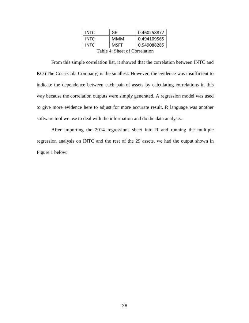
Company Company Correlation INTC KO 0.163379529 INTC AAPL 0.216856382 INTC V 0.217627613 INTC NKE 0.220008633 INTC HD 0.222552133 INTC PG 0.228610937 INTC MRK 0.265253872 INTC MCD 0.27500614 INTC WMT 0.280123692 INTC TRV 0.280719747 INTC UTX 0.293778755 INTC UNH 0.295207306 INTC VZ 0.306220831 INTC PFE 0.307461828 INTC DD 0.309532287 INTC IBM 0.311483727 INTC JNJ 0.3175937 INTC CVX 0.32145425 INTC BA 0.324174314 INTC CAT 0.334473464 INTC DIS 0.352877496 INTC XOM 0.360204204 INTC GS 0.393399476 INTC AXP 0.403812028 INTC JPM 0.427715217 INTC CSCO 0.460201611

28

INTC GE 0.460258877 INTC MMM 0.494109565 INTC MSFT 0.549088285

Table 4: Sheet of Correlation

From this simple correlation list, it showed that the correlation between INTC and

KO (The Coca-Cola Company) is the smallest. However, the evidence was insufficient to

indicate the dependence between each pair of assets by calculating correlations in this

way because the correlation outputs were simply generated. A regression model was used

to give more evidence here to adjust for more accurate result. R language was another

software tool we use to deal with the information and do the data analysis.

After importing the 2014 regressions sheet into R and running the multiple

regression analysis on INTC and the rest of the 29 assets, we had the output shown in

Figure 1 below:

29

Figure 1: R call output of model1

The p-value ( Pr > |t| in the lm output) tests the null hypothesis that the

coefficient is 0 versus the alternative hypothesis that it is not 0. If a p-value for a predictor

variable is small, then it shows evidence that the predictor has a linear relationship with

the response variable. (Ruppert, 2011)

From the output we saw that the p-value (Pr > |t| in the lm output) of MSFT was

the smallest among all the other p-values, in this case, we concluded that this was

evidence that the coefficient of MSFT was not 0 and MSFT had a linear relationship with

the response INTC. Also, it was most correlated to INTC compared to the other assets.

Therefore, we ran the multiple regressions to model the relationship between

30

MSFT and the rest of the 28 assets to find the most correlated one to MSFT, exactly the

same as what we did before when we ran the regression analysis. We repeated the

procedure until there was only one asset left which was the least correlated to the INTC

asset. Every time the predictor with the smallest p-value had to be eliminated, as it is the

most correlated to the corresponding response variable, thus leaving the least correlated

predictor in the rest of the predictors. The R codes are shown in Figure 2 below.

Figure 2: multiple linear regressions (R codes)

Model 1 through model 29 stand for all the 29 multiple regressions models on the

corresponding assets. From the outputs we got, we concluded that AAPL (Apple Inc.) was

the one we were looking for, which was the least correlated to INTC since it was the last

asset left after we did all 29 attempts. Therefore, AAPL was the second risky asset we

figured out how to combine with INTC to find the efficient portfolio.

3.1.3 Model Diagnostics

After we fitted the regression model, it was important to determine if the models

were normal to ensure the assumptions were valid. Since AAPL was the least dependent

to INTC among the rest of the 29 securities, we performed the model diagnostic on AAPL

31

and INTC. We assigned model=lm(INTC~AAPL) in R and plotted the model in Figure 3

below.

Figure 3: Diagnostics in R: Plot (model)

We saw from the plots, there were three outliers and all of them were significantly

bigger than the majority, which definitely made the overall expected return bigger than

normal. Thus, we removed the outliers to make it normal since the outliers may result in a

faulty conclusion. After we removed the three outliers, we had the new plots Figure 4

below.

32

Figure 4: Diagnostics in R: plot (model.2)

After removing the outliers, to avoid violations in the current model, the 112th,

135th and 195th data from the excel sheet to refresh the expected return from INTC and

AAPL before we began the next procedure asset allocation.

Company Expected Return Volatility INTC 0.000473212 0.005041186 AAPL 0.000656052 0.005945869

Table 5: Update Return and Risk of 2 risky assets

After we updated the expected return and risk, it was clear that the expected return

33

of INTC decreases from 0.000644984 to 0.000473212 as some of the outliers had

unrealistically large returns, which may have resulted in inaccurate estimates.

3.2 Asset Allocation

3.2.1 Transferring the Risk-free Rate

The following figure shows the raw data of the two risky assets and the risk-free

asset we chose.

Company Expected Return Volatility INTC 0.000473212 0.005041186 AAPL 0.000656052 0.005945869 Risk-free rate 0.001210843 0.000343727

Table 6: Return and Risk sheet of two Risky Assets and Risk-free Asset

The risk-free rate we choose is daily Treasury Yield Curve 1-year Rate, so the

expected return is the annual rate. To unify the risk-free asset and risky assets, we need to

transfer the risk-free rate into daily rate. Suppose the annual risk-free rate is 𝜇𝜇𝑓𝑓𝑓𝑓 then

using the formula

𝜇𝜇𝑓𝑓𝑑𝑑 = (1 + 𝜇𝜇𝑓𝑓𝑓𝑓)1/365 − 1

to obtain the daily rate.

Thus 𝜇𝜇𝑓𝑓𝑑𝑑 = (1 + 0.00121260163)1/365 − 1 = 3.31538E-06 as shown in Table 7

below.

Company Expected Return Volatility (std of dif adj close) INTC 0.000473212 0.005041186 AAPL 0.000656052 0.005945869 Risk-free rate 3.31538E-06 0.000343727

Table 7: Daily Return and Risk sheet

34

3.2.2 Tangency Portfolio

By using the Formula 2.8 in the previous chapter we developed to find the weight

for tangency portfolio.

𝑤𝑤𝑇𝑇 =𝑉𝑉1𝜎𝜎22 − 𝑉𝑉2𝜌𝜌12𝜎𝜎1𝜎𝜎2

𝑉𝑉1𝜎𝜎22 + 𝑉𝑉2𝜎𝜎12 − (𝑉𝑉1 + 𝑉𝑉2)𝜌𝜌12𝜎𝜎1𝜎𝜎2

where the excess expected returns 𝑉𝑉1 = 𝜇𝜇1 − 𝜇𝜇𝑓𝑓 and 𝑉𝑉2 = 𝜇𝜇2 − 𝜇𝜇𝑓𝑓 .

We obtain 𝑉𝑉1 = 0.000469897,𝑉𝑉2 =0.000652736 and weight 𝑤𝑤𝑇𝑇 = 0.47752457

by inputting the formulas into Excel shown in Table 8 below.

Cor 0.216856382 V1 0.000469897 V2 0.000652736

1.23696E-08 2.59036E-08

Wt 0.47752457 1-Wt 0.52247543 E(Rt) 0.000568741 std 0.004323113 Table 8: Tangency Portfolio weight

3.4163E-09 and 1.10813E-08 are numerator 𝑉𝑉1𝜎𝜎22 − 𝑉𝑉2𝜌𝜌12𝜎𝜎1𝜎𝜎2 and denominator 𝑉𝑉1𝜎𝜎22 +

𝑉𝑉2𝜎𝜎12 − (𝑉𝑉1 + 𝑉𝑉2)𝜌𝜌12𝜎𝜎1𝜎𝜎2 which help to obtain the weight.

By the Formulas 2.9

𝐸𝐸(𝑅𝑅𝑇𝑇) = 𝑤𝑤𝑇𝑇𝜇𝜇1 + (1 − 𝑤𝑤𝑇𝑇)𝜇𝜇2

and the Formulas 2.10

𝜎𝜎𝑇𝑇 = �𝑤𝑤𝑇𝑇2𝜎𝜎12 + (1 − 𝑤𝑤𝑇𝑇)2𝜎𝜎22 + 2𝑤𝑤𝑇𝑇(1 − 𝑤𝑤𝑇𝑇)𝜌𝜌12𝜎𝜎1𝜎𝜎2

from Chapter 2, we calculated the return and standard deviation of the tangency portfolio

which are 0.000568741 and 0.004323113 respectively. The standard deviation of

tangency portfolio is smaller than both of INTC and AAPL, and the overall expected

35

return is between those of INTC and AAPL. Therefore, we reduced the risk level and

maintained the expected return after combining these two assets into the tangency

portfolio shown in Table 9 below.

Daily INTC AAPL Risk free rate Tangency portfolio MEAN 0.047% 0.066% 0.00033% 0.057% STD 0.504% 0.595% 0.034% 0.432%

Table 9: Daily Tangency Portfolio output

We had our tangency portfolio combined by 47.75% of INTC and 52.25% of

AAPL.

3.3 Portfolio Optimization

After finding the tangency portfolio, which ensures the highest expected return

between two risky assets with minimum risk by choosing the tangency weight 𝑤𝑤𝑇𝑇, the

next step was to find the combing fraction 𝜔𝜔 between the risk-free asset and tangency

portfolio we got to obtain the ultimate portfolio. Before that, we wanted to annualize all

the outputs in order to do the following procedures more conveniently. The annualized

data are shown in Table 10 below.

Annual INTC AAPL Risk free rate Tangency Portfolio MEAN 18.849% 27.046% 0.121% 23.064% STD 7.955% 9.382% 0.542% 6.822%

Table 10: Annualized return and risk output

We needed to set up our goals first to combine our two risky assets with the risk-

free asset. We could set our target in various ways: ensuring a high-expected return, or

ensuring a low risk level.

36

3.3.1 Targeting a Certain Expected Return

Suppose we wanted a 20% expected return, firstly, we needed to transfer 20%

annual return into daily return which was (1.2)1/365 − 1 = 0.0004996359.

We assigned 𝐸𝐸(𝑅𝑅𝑃𝑃) = 0.000568741, then, substituted the 𝜇𝜇𝑓𝑓 and 𝐸𝐸(𝑅𝑅𝑇𝑇) into the

Formula 2.11 from Chapter 2, we obtained 0.877781468. According to 𝜎𝜎𝑅𝑅𝑃𝑃 = 𝜔𝜔𝜎𝜎𝑇𝑇 , we

could also get the standard deviation of the ultimate portfolio 𝜎𝜎𝑅𝑅𝑃𝑃 =5.988%.

Identically, if we wanted a lower expected return such as 15%, corresponding to a

0.0003829 daily return, and substituted the data into the formula, we got 𝜔𝜔 =

0.671471307 and 𝜎𝜎𝑅𝑅𝑃𝑃 = 4.581%. Thus, if we lowered the expected return, the weight

would decrease and standard deviation would decrease. Since 𝜔𝜔 was the fraction of the

ultimate investment to the tangency portfolio with an optimal expected return, the smaller

the targeted return, the smaller the fraction 𝜔𝜔 would be. Once the expected return

decreased, the relative risk level would decrease.

3.3.2 Targeting Certain Volatility

Another option was to reduce the risk level and maintain the return as much as

possible. Suppose we were targeting the volatility to be 6% (our current tangency risk was

6.822%) then used the formula (2.11)

𝜎𝜎𝑅𝑅𝑃𝑃 = 𝜔𝜔𝜎𝜎𝑇𝑇 .

We neglected the risk of risk-free asset, as the standard deviation was really small.

Therefore,

𝜔𝜔 =𝜎𝜎𝑅𝑅𝑃𝑃𝜎𝜎𝑇𝑇

=0.06

0.06822= 0.879538674.

𝜔𝜔 was relatively big, since our targeted volatility was close to the that of tangency

37

portfolio. We could obtain the expected return 20.044%

Next, we changed our target to 5% volatility annually. Then

𝜔𝜔 =𝜎𝜎𝑅𝑅𝑃𝑃𝜎𝜎𝑇𝑇

=0.05

0.06822= 0.732948895.

Since the weight was still beyond a half, there was space to lower the risk.

𝐸𝐸(𝑅𝑅𝑃𝑃) = 16.468%.

If we chose the volatility to be 2.5%,

𝜔𝜔 =𝜎𝜎𝑅𝑅𝑃𝑃𝜎𝜎𝑇𝑇

=0.025

0.06822= 0.366474447.

and

𝐸𝐸(𝑅𝑅𝑃𝑃) = 7.986%

The weight was half of the previous weight corresponding to 𝜎𝜎𝑅𝑅𝑃𝑃 = 0.05, as the

volatility was also half of the previous one.

We had five different outputs based on the corresponding targets shown in Table

11 below.

Combing portfolio Portfolio 1 Portfolio 2 Portfolio 3 Portfolio 4 Portfolio 5 MEAN 15.000% 20.000% 7.986% 16.468% 20.044% STD 4.581% 5.988% 2.500% 5.000% 6.000% w 0.671471307 0.877781468 0.366474447 0.732948895 0.879538674

Table 11: Combined Portfolio Outputs

The first two columns of the form show the outputs when we assigned our target

to be expected return and the last three show the results based on the certain volatility

target. If we combined them together, and looked at the return and volatility, we could get

the conclusion that small return was always followed by a relatively small risk level, and

the corresponding proportion to the tangency portfolio was small. As the expected return

38

increased, the volatility increased and combined weight increased at the same level.

To see the ultimate combined portfolio more clearly, we plot the portfolio into R

in Figure 5 shown below.

Figure 5: Portfolio plots (R)

These four plots correspond to the combined portfolio1, 3, 4, 5. We can see from

the graph that the portfolio with 𝜔𝜔 = 0.8795 earned higher return under a relatively high

risk level. To better understand the portfolio and refine the best one, we used the next

chapter-performance measurement.

39

3.4 Performance Measurement

3.4.1 Value-at-Risk

In financial risk management, VaR is always used to measure risk of loss on a

given period. We used VaR to see the loss value based on the confidence level of 99%

and 95%. The output is shown in Table 12 below.

VaR at 1000000 INTC AAPL Tangency portfolio 0.99 -11254.33999 -13176.10766 -9488.324437 0.95 -7818.800709 -9124.032255 -6542.147466

Table 12: VaR of portfolio

From the form, it shows that there is a one-day 1% chance that the tangency

portfolio will fall in value by more than $9488 and one-day 5% chance that the tangency

portfolio will fall in value by more than $6542 based on a $1 million investment, which is

good to see since it is much lower than both of VaR of INTC and AAPL.

3.4.2 Sharpe Ratio

As we talked in the previous chapter, the Sharpe Ratio calculates the average

return earned in excess of the risk-free rate per unit of volatility. The greater the value of

the Sharpe Ratio, the better the performance of the risk-adjusted return. Thus, Sharpe

Ratio is another way to measure the performance of our investment.

Firstly, we calculated the Sharpe Ratio of the initial assets and the tangency

portfolio to check whether our tangency portfolio was doing well by using the formula

(2.12)

𝑆𝑆ℎ𝑎𝑎𝑟𝑟𝑝𝑝𝑎𝑎 𝑟𝑟𝑎𝑎𝑡𝑡𝑟𝑟𝑜𝑜 =𝐸𝐸(𝑅𝑅𝑃𝑃) − 𝜇𝜇𝑓𝑓

𝜎𝜎𝑅𝑅𝑃𝑃

40

We got that the Sharpe ratio of INTC was 2.354245593, of AAPL was

2.869736534, and tangency portfolio was 3.36314739. Hence, the tangency portfolio had

a Sharpe ratio larger than both of AAPL and INTC, which indicates our tangency

portfolio was performing well so far.

After that, we tested our five combined portfolios to see which one earned the

most return in excess of the risk-free rate per unit of the total risk. We subsequently got

the Sharpe ratio of these portfolios shown in Table 13 below.

Combing portfolio Portfolio 1 Portfolio 2 Portfolio 3 Portfolio 4 Portfolio 5 MEAN 15.000% 20.000% 7.986% 16.468% 20.044% STD 4.581% 5.988% 2.500% 5.000% 6.000% w 0.671471307 0.877781468 0.366474447 0.732948895 0.879538674 Sharpe ratio 3.248235531 3.319785115 3.146130641 3.269342821 3.320403358

Table 13: Sharpe ratio outputs

From the form, we saw that even all the five Sharpe ratios were close to each

other, but the Sharpe ratio of the last column was the biggest with the value 3.3204.

Therefore, we gave a preliminary conclusion that the portfolio 5 with mean of 20.044%

and standard deviation of 6% was the best among all the others.

3.4.3 Sortino Ratio

From the log return of two assets, we saw nearly half of them were negative. In

this case, we should also look at the Sortino ratio besides the Sharpe ratio.

The Sortino ratio always focuses on the standard deviation of negative asset

returns, which is also called downside deviation. In this case, the Sortino ratio analyzes

the portfolio with relatively high volatility better than the Sharpe ratio.

To calculate the Sortino ratio, we needed to measure the downside deviation of the

portfolio. First of all, we filtered data by choosing “less than 0” command, and pasted all

41

the negative returns into the new column. After that, we calculated the standard deviation

of these negative returns. The downside deviations of INTC and AAPL were

0.033389943 and 0.048243976. The pairwise covariance between INTC and AAPL was -

7.02887E-07, it means the dependence was very weak and they were almost independent.

Hence, we can use the formula

𝑠𝑠𝑜𝑜𝑟𝑟𝑡𝑡𝑟𝑟𝑠𝑠𝑜𝑜 𝑟𝑟𝑎𝑎𝑡𝑡𝑟𝑟𝑜𝑜 = 𝐸𝐸(𝑅𝑅𝑃𝑃)− 𝜇𝜇𝑓𝑓

𝜎𝜎𝑑𝑑

to find the ultimate downside deviation 0.029825909. The results are shown in Table 14

below.

Combing portfolio Portfolio 1 Portfolio 2 Portfolio 3 Portfolio 4 Portfolio 5 MEAN 15.000% 20.000% 7.986% 16.468% 20.044% STD 4.581% 5.988% 2.500% 5.000% 6.000% w 0.671471307 0.877781468 0.366474447 0.732948895 0.879538674 Sharpe ratio 3.248235531 3.319785115 3.146130641 3.269342821 3.320403358 Sotino ratio 4.988587566 6.664982432 2.637078627 5.480709521 6.679568571

Table 14: Sortino ratio outputs

The Sortino ratio manifested the same conclusion that the portfolio 5 was the best among

the five portfolios and made it more evident.

In conclusion, we acquired our most desirable combined portfolio with annual

return of 20.044% and risk of 6.00%. So 12.05% of the portfolio should be in the risk-free

asset, and 87.95% should be in the tangency portfolio. Therefore, 42% should be in the

first asset INTC and 45.95% should be in the second asset AAPL. The total was around

100%. The result is shown in Table 15 below.

Combing portfolio Tangency Portfolio

Portfolio 1 Portfolio 2 Portfolio 3 Portfolio 4 Portfolio 5 Tangency Portfolio

MEAN 15.000% 20.000% 7.986% 16.468% 20.044% 23.064%

42

STD 4.581% 5.988% 2.500% 5.000% 6.000% 6.822%

w 0.671471307

0.877781468

0.366474447

0.732948895

0.879538674 1

Sharpe ratio

3.248235531

3.319785115

3.146130641

3.269342821

3.320403358

3.363147390

Sotino ratio

4.988587566

6.664982432

2.637078627

5.480709521

6.679568571

7.692163885

Table 15: The overall performance measurement

If we put the combined portfolios and tangency portfolio together, we saw that the

tangency portfolio had a better performance result analysis than any of the combined

portfolio. As the Sharpe ratio and the sortino ratio were also used to compare the change

in a portfolio’s overall risk-return characteristics when a new asset was added into the

portfolio, if the addition of the new investment lowers the ratio, it means it should not be

added to the portfolio. In this case, the addition of the risk-free asset did lower both of the

two ratios, and the two risky assets were doing well in 2014, combing INTC and AAPL

with the risk-free asset was not a good option for investment comparing to the tangency

portfolio. Our final solution was choosing the tangency portfolio instead of combing the

tangency with risk-free asset for investment.

3.5 INTL and KO

From the correlation list in the previous section, we found that the correlation between

INTC and KO (The Coca-Cola Company) is the even smaller than INTC and AAPL. In

this case, to certify our conclusion that INTC and AAPL is the best tangency portfolio

combination, we are going to combine INTL and KO and risk-free asset in this section.

Since we have done the procedures, it is familiar to us. We restarted everything

performing the model diagnostic on KO and INTC. We assigned model0=lm(INTC~KO)

43

in R and plot model in Figure 6 below.

Figure 6: Diagnostics in R (INTC~ KO)

INTC~KO had same outliers with INTC~AAPL as we expect, as these outliers

were extremely large return in INTC. Then, we removed the outliers as shown in Figure 7

below.

44

Figure 7: Plot INTC~KO without outliers

We updated the return and risk sheet in EXCEL shown in Table 16 below.

Company Expected Return Volatility INTC 0.000473212 0.005041186 KO 9.51939E-05 0.004120615 Risk-free rate 0.001210843 0.000343727

Table 16: Return and Risk sheet (INTC&KO)

After preliminary analyzing this return and risk sheet, the expected return of KO

was much lower than that of AAPL and really close to 0, we gave an assumption that the

expected return of this tangency portfolio was lower than the tangency portfolio of INTC

45

and AAPL. In the following process, we will prove this assumption. The tangency

portfolio output is shown in Table 17 below.

Cor 0.163379529 V1 0.000469897 V2 9.18785E-05

7.66678E-09 8.40698E-09

w 0.911954041 1-w 0.088045959 E(Rt) 0.000439929 std 0.00467034 Table 17: Tangency portfolio outputs (INTC&KO)

The weight for this tangency portfolio we got was really close to 1, which means

that the proportion of INTC in the portfolio is really high since the return of the two asset

are quite different. We attach the annual return and risk sheet for INTC&KO shown in

Table 18 below.

Annual INTC KO Risk free rate Tangency Portfolio MEAN 18.85% 3.54% 0.1211% 17.41% STD 7.955% 6.502% 0.542% 7.370%

Table 18: Annualized return and risk outputs (INTC&KO)

The expected return of the portfolio combined by INTC and KO (17.41%) was

much lower than the expected return of the portfolio combined by INTC and AAPL

(23.064%) and the volatility (7.37%) was higher than the volatility of INTC and AAPL

(6.822%) which was not a good option to choose to combine. To make it clear, we

calculated the Sharpe ratio of both of the tangency portfolio in Figure 25 below.

Annual Tangency Portfolio (INTC&AAPL)

Tangency Portfolio (INTC&KO)

MEAN 23.06% 17.41% STD 6.82% 7.37% Sharpe ratio 3.36314739 2.346544215

Table 19: Performance measurement output

46

From the sheet, it is clear that the Sharpe ratio of the tangency portfolio consisted of

INTC & AAPL is larger than the tangency portfolio consisted of INTC & KO.

In conclusion, INTC and AAPL is the best combination to be the tangency

portfolio, and the combined portfolio we found in 3.4 is the best among all the combined

portfolios. According to the performance analysis, the tangency portfolio of AAPL and

INTC is the most desirable portfolio in terms of reward-to-risk criteria for investment.

47

Chapter 4

Conclusion

In this project, we focus on risk management, regression analysis and portfolio

theory. We applied regression analysis to find a pair of two risky assets from Dow Jones

30 companies with highest return and lowest risk and found the proportion of the two

assets to combine them into the tangency portfolio. We applied several reward-to-risk

measures including Value-at-Riak, Sharpe ratio and Sortino ratio to evaluate the

performance of our portfolios. Finally, we obtained our most desirable portfolio in terms

of reward-to-risk criteria for investment.

4.1 Results Summary

At first, the data we chose in 2015 was not good for the asset portfolio

combination since during the time, the stock market was experiencing a downturn trend

and undertaking enormous risks. Therefore, we reorganized the assets into 2014 and

generalized them again from Yahoo Finance.

After that, we found the pair of assets with maximum return and minimum risk by

seeking out the asset INTC with the highest return and it least correlated asset AAPL after

performing 30 attempts of regression models through R. In addition, we ran model

diagnostics on the regression models to reduce the existing error. Then, we applied

portfolio theory to find the weight for the tangency portfolio between INTC and AAPL

and the combined portfolio based on the certain targets. Finally, we used several measures

to estimate the performance of our combined portfolios and tangency portfolio to

determine our best portfolio for investing.

48

After all the data analysis and the use of the Sharpe ratio and the Sortino ratio to

measure the overall performance of all the portfolios we combined, we decided that the

tangency portfolio of INTC and AAPL constitute the most desirable portfolio we were

seeking with allocation distribution as 47.75% of INTC and 52.25% of AAPL. Since the

status of stock market was strong in 2014. Adding the risk-free asset into the tangency

portfolio lowers the Sharpe ratio and Sortino ratio, therefore, we recommend that the

tangency portfolio without the risk-free asset is preferable if the maximum return is the

ultimate goal.

4.2 Future Work

There is no doubt that people have a lot to be done in the field of risk management,

especially the portfolio theory. By extending the method of finding the optimal

compromise between expected return and risk, detailed in the Methodology Section, we

can also find the efficient portfolios with an arbitrary number of assets instead of two

risky assets and one risk-free asset. We can add more assets into the portfolio to see if

there is more room to improve the investment. More details can be found in e.g., Ruppert,

2011, Chapter 11.

Risk management is rapidly developing into an essential strategic approach in the

recent decades. Generally, riskier investments have a higher expected return, as investors

always demand a reward for bearing higher risk. In this case, risk management is crucial

to either short-term trends or long-term development.

49

Appendix A:

R code

mu1 = 0.26534287 mu2 = 0.251289796 sig1 = 0.09538 sig2 = 0.08665 rho = 0 rf = 0.001210843 corr = 0.216856382 w = seq(0, 1, len = 500) means = 0.26534287 * w + 0.251289796 *(1-w) var = sig1^2 * w^2 + sig2^2 * (1 - w)^2 + 2 * w * (1-w) * corr *sig1 *sig2 risk = sqrt(var) ind = !(risk > min(risk)) ind2 = (means > means[ind]) wt = 0.509182468 meant = 0.26534287 * wt + 0.251289796 * (1-wt) riskt = sqrt(sig1^2 * wt^2 + sig2^2 * (1 - wt)^2 + 2 * wt * (1-wt) * corr *sig1 *sig2) wp = 0.411467822 meanp = wp * meant + (1- wp) * rf riskp = wp * riskt #pdf("portfolioNew.pdf", width = 6, height = 5) plot(risk, means, type = "l", lwd = 1, xlim = c(0, 0.1), ylim = c(0.0010, 0.27)) abline(v = 0) lines(risk[ind2], means[ind2], type = "l", lwd = 5, col = "red") lines( c(0, riskt), c(rf, meant), col = "blue", lwd =2) lines(c(0,riskp), c(rf,meanp), col = "purple", lwd = 2, lty = 2) text(riskt, meant, "T", cex = 1) text(sig1, mu1, "R1", cex = 1) text(sig2, mu2, "R2", cex = 1) text(0, rf, "F", cex = 1) text(riskp, meanp, "P", cex = 1) text(min(risk), means[ind], "MV", cex = 1) #graphics.off()

50

data=read.table(file.choose(),header=T,sep=",") attach(data) View(data) model1=lm(INTC~MMM+AXP+AAPL+CAT+CVX+CSCO+DD+XOM+GE+IBM+JNJ+JPM+MCD +MRK+MSFT+NKE+PFE+BA+KO+GS+HD+PG+TRV+DIS+UTX+UNH+VZ+V+WMT) model2=lm(MSFT~MMM+AXP+AAPL+CAT+CVX+CSCO+DD+XOM+GE+IBM+JNJ+JPM+MCD +MRK+NKE+PFE+BA+KO+GS+HD+PG+TRV+DIS+UTX+UNH+V+WMT+VZ) model3=lm(VZ~MMM+AXP+AAPL+CAT+CVX+CSCO+DD+XOM+GE+IBM+JNJ+JPM+MCD +MRK+NKE+PFE+BA+KO+GS+HD+PG+TRV+DIS+UTX+UNH+V+WMT) model4=lm(XOM~MMM+AXP+AAPL+CAT+CVX+CSCO+DD+GE+IBM+JNJ+JPM+MCD+MRK +NKE+PFE+BA+KO+GS+HD+PG+TRV+DIS+UTX+UNH+V+WMT) model5=lm(CVX~MMM+AXP+AAPL+CAT+CSCO+DD+GE+JNJ+IBM+JPM+MCD+MRK+NKE +PFE+BA+KO+GS+HD+PG+TRV+DIS+UTX+UNH+V+WMT) model6=lm(CAT~MMM+AXP+AAPL+CSCO+DD+GE+JNJ+IBM+JPM+MCD+MRK+NKE+PFE +BA+KO+GS+HD+PG+TRV+DIS+UTX+UNH+V+WMT) model7=lm(UTX~MMM+AXP+AAPL+CSCO+DD+GE+JNJ+IBM+JPM+MCD+MRK+NKE+ +BA+KO+GS+HD+PG+TRV+DIS+UNH+V+WMT) model8=lm(BA~MMM+AXP+AAPL+CSCO+DD+GE+JNJ+IBM+JPM+MCD+MRK+NKE+PFE +KO+GS+HD+PG+TRV+DIS+UNH+V+WMT) model9=lm(MMM~AXP+AAPL+CSCO+DD+GE+JNJ+IBM+JPM+MCD+MRK+NKE+PFE+KO +GS+HD+PG+TRV+DIS+UNH+V+WMT) model10=lm(GE~AXP+AAPL+CSCO+DD+JNJ+IBM+JPM+MCD+MRK+NKE+PFE+KO +GS+HD+PG+TRV+DIS+UNH+V+WMT) model11=lm(CSCO~AXP+AAPL+DD+JNJ+IBM+JPM+MCD+MRK+NKE+PFE+KO +GS+HD+PG+TRV+DIS+UNH+V+WMT) model12=lm(IBM~AXP+AAPL+DD+JNJ+JPM+MCD+MRK+NKE+PFE+KO +GS+HD+PG+TRV+DIS+UNH+V+WMT) model13=lm(JNJ~AXP+AAPL+DD+JPM+MCD+MRK+NKE+PFE+KO +GS+HD+PG+TRV+DIS+UNH+V+WMT) model14=lm(MRK~AXP+AAPL+DD+JPM+MCD+NKE+PFE+KO +GS+HD+PG+TRV+DIS+UNH+V+WMT) model15=lm(PFE~AXP+AAPL+DD+JPM+MCD+NKE+KO +GS+HD+PG+TRV+DIS+UNH+V+WMT) model16=lm(V~AXP+AAPL+DD+JPM+MCD+NKE+KO +GS+HD+PG+TRV+DIS+UNH+WMT) model17=lm(AXP~AAPL+DD+JPM+MCD+NKE+KO +GS+HD+PG+TRV+DIS+UNH+WMT) model18=lm(GS~AAPL+DD+JPM+MCD+NKE+KO+HD+PG+TRV+DIS+UNH+WMT) model19=lm(JPM~AAPL+DD+MCD+NKE+KO+HD+PG+TRV+DIS+UNH+WMT) model20=lm(TRV~AAPL+DD+MCD+NKE+KO+HD+PG+DIS+UNH+WMT) model21=lm(DD~AAPL+MCD+NKE+KO+HD+PG+DIS+UNH+WMT) model22=lm(DIS~AAPL+MCD+NKE+KO+HD+PG+UNH+WMT) model23=lm(NKE~AAPL+MCD+KO+HD+PG+UNH+WMT) model24=lm(HD~AAPL+MCD+KO+PG+UNH+WMT)

51

model25=lm(WMT~AAPL+MCD+KO+PG+UNH) model26=lm(PG~AAPL+MCD+KO+UNH) model27=lm(KO~AAPL+MCD+UNH) model28=lm(MCD~AAPL+UNH) model29=lm(UNH~AAPL) model=lm(INTC~AAPL) par(mfrow=c(2,2)) plot(model) model.2=lm(UNH[-c(134,112,195)]~AAPL[-c(134,112,195)]) plot(model.2)

52

Appendix B:

Excel Sheets

Annualized Return and Risk

Annual INTC AAPL Tangency Portfolio MEAN 18.849% 27.046% 23.064% STD 7.955% 9.382% 6.822% Sharpe's ratio 2.35424559 2.86973653 3.36314739

Downside Deviation output

INTC AAPL Portfolio Downside Deviation 0.033389943 0.048243976 0.029825909

Performance Measurement of portfolios

Combing portfolio Tangency Portfolio

Portfolio 1 Portfolio 2 Portfolio 3 Portfolio 4 Portfolio 5

Tangency Portfolio

MEAN 15.000% 20.000% 7.986% 16.468% 20.044% 23.064% STD 4.581% 5.988% 2.500% 5.000% 6.000% 6.822% w 0.67147 0.8777814 0.3664744 0.7329488 0.8795386 1 Sharpe ratio

3.248235531

3.319785115

3.146130641

3.269342821

3.320403358

3.363147390

Sotino ratio

4.988587566

6.664982432

2.637078627

5.480709521

6.679568571

7.692163885

VaR at 99% -6370.04 -8328.27 -3475.13 -6953.57 -8344.95 -9488.32 VaR at 95% -4391.78 -5742.17 -2395.43 -4794.17 -5753.67 -6542.15

53

Bibliography

[1] Ruppert, D. (2011). Statistics and data analysis for financial engineering. Springer,

New York.

[2] Ruppert, D. (2004). Statistics and finance: An introduction. Springer, New York.

[3] Legendre, A.M. (1805). Nouvelles Méthodes Pour La Détermination Des Orbites

Des Comètes. Chez Firmin Didot.

[4] Gauss, C.F. (1809). Theoria Motus Corporum Coelestium in Sectionibus Conicis

Solem Ambientum.

[5] Gauss, Carl Friedrich. (1821). Theoria Combinationes Observationum Erroribus

Minimis Obnoxia.

[6] Galton, Francis. (1989). "Kinship and Correlation." Statistical Science Statist. Sci.:

81-86.

[7] Yule, G. Udny. (1897). “On the Theory of Correlation.” Journal of the Royal

Statistical Society: 812-854.

[8] Pearson, Karl; Yule, G. U.; Blanchard, Norman; and Lee, Alice. (1903). "The Law of

Ancestral Heredity." Biometrika: 211-228.

[9] Markowitz, H. (1959). Portfolio Selection: Efficient Diversification of Investment.

Wiley, New York.

[10] Miller, Kent D. (1992). "A Framework for Integrated Risk Management in

International Business." Journal of International Business Studies J Int Bus Stud: 311-31.

54

[11] Slovic, Paul. (2000). The Perception of Risk. Earthscan Publications, London.

[12] Ross, Stephen A. (1976). "The Arbitrage Theory of Capital Asset Pricing." Journal

of Economic Theory: 341-60.

[13] Roll, Richard; Ross, Stephen. (1980). "An Empirical Investigation of the Arbitrage

Pricing Theory." The Journal of Finance: 1073.

[14] Fama, Eugene F., and Kenneth R. French. (1993). "Common Risk Factors in the

Returns on Stocks and Bonds." Journal of Financial Economics: 3-56.

[15] Fama, E. F., & French, K. R. (1992). The cross‐ section of expected stock

returns. the Journal of Finance, 47(2), 427-465.

[16] Fama, E. F., & French, K. R. (2004). The capital asset pricing model: Theory and

evidence. Journal of Economic Perspectives, 18, 25-46.

[17] Sharpe, W. F. (1966). “Mutual Fund Performance.” Journal of Business: 119-138.

[18] Sortino, Frank Alphonse. (2010). The Sortino Framework for Constructing

Portfolios Focusing on Desired Target Return to Optimize Upside Potential Relative to

Downside Risk. Elsevier, Amsterdam.

[19] Chang, Chia. Jiménez-Martin, Juan-Angel. McAleer, Michael. Amaral, Teodosio.

(2011). Risk Management of Risk under the Basel Accord Forecasting Value-at-risk of

VIX Futures. N.Z.: Dept. of Economics and Finance, College of Business and Economics,

U of Canterbur, Christchurch.

[20] Sortino, Frank Alphonse. (2001). Managing Downside Risk in Financial Markets

Theory, Practice and Implementation. Butterworth-Heinemann, Oxford.

[21] Pindyck, Robert S., and Daniel L. Rubinfeld. (1981). Econometric Models and

Economic Forecasts. 2d ed. McGraw-Hill, New York.

55

[22] MacAleer, Michael, and Juan Martin. (2009). Has the Basel II Accord Encouraged

Risk Management during the 2008-09 Financial Crisis? [etc.: Tinbergen Institute,

Amsterdam.

[23] Chen, N. F., Roll, R., & Ross, S. A. (1986). “Economic forces and the stock

market.” Journal of business, 383-403.

[23] Dodge, Y. (2003). The Oxford Dictionary of Statistical Terms. 6th ed. Oxford UP,

Oxford.

[24] Jensen, M. C., Black, F., & Scholes, M. S. (1972). “The capital asset pricing model:

Some empirical tests.” Studies in the Theory of Capital Markets.

[25] Elton, Edwin J., and Gruber, Martin J. (1998). Modern Portfolio Theory: 1950 to

Date. NYU Stern, New York.

[26] Frencha C W. (2003). The Treynor capital asset pricing model. Journal of

Investment Management, 1(2): 60-72.