a statistical method for maximum power estimation …

Active and Pasaive Elec. Comp., 2000, Vol. 22, pp. 215-233 (C) 2000 OPA (Overseas Publishers Association) N.V.Reprints available directly from the publisher Published by license underPhotocopying permitted by license only the Gordon and Breach Science

Publishers imprint.Printed in Singapore

A NEW STATISTICAL METHODFOR MAXIMUM POWER ESTIMATION

IN CMOS VLSI CIRCUITS

N. E. EVMORFOPOULOS and J. N. AVARITSIOTIS*

Department of Electrical and Computer Engineering, NationalTechnical University of Athens, 9, Iroon Polytechniou St.,

Zographou, Athens, 15773, Greece

(Received 11 October 1999; In finalform 18 November 1999)

A method for maximum power estimation in CMOS VLSI circuits is proposed. Themethod is based on extreme value theory and allows for the calculation of the upper endpoint of the probability distribution which is followed by the instantaneous power drawnfrom the supply bus. The main features of the method arc the relatively small and circuit-independent subset of input patterns required for accurate prediction of maximumpower and its simulative nature which ensures that no over-simplifying assumptions arcmade. Application of the proposed method to eight distributions, which come close tothe behavior of power consumption in VLSI circuits, proved its superior capabilitieswith respect to existing methods.

Keywords: Maximum power; reliability; CMOS VLSI circuits; statistics; extremes

1. INTRODUCTION

Excessive instantaneous power dissipation in CMOS VLSI circuitsis a potential source of many reliability and performance problemssuch as physical failures duc to overheating or clcctromigration, func-tional failures caused by voltage drop (or IR-drop) on power rails,reduced noise margins and switching speed degradation. The issuesregarding reliability arc becoming cvcn more important as we moveinto dccp-submicron ICs which exhibit decreased feature sizes and

*Corresponding author, e-mail: [email protected]

215

216 N.E. EVMORFOPOULOS AND J. N. AVARITSIOTIS

power supply levels. Consequently, there is an increasing need fortools and methods that perform fast and accurate estimation of thecircuit’s maximum power requirements during the design phase.

Previous work on this field has focused on the creation and ex-ploitation of deterministic or stochastic information (such as switch-ing activity and signal correlations) about the circuit’s inputs, withoutexplicitly simulating the circuit. While most related techniques exhibitgood timing figures, they make some simplifying assumptions that of-ten result in loss of accuracy. In addition, their speed and algorithmicefficiency generally degrade with large or complex circuit structures.Statistical methods might offer a promising alternative but they havenot seen a widespread application as yet, due to the inadequacy of exist-ing statistical models to deal with extreme situations such as in maxi-mum power analysis. Even though a step towards the right direction wasmade in [1], the reported method overlooked some important factsabout extremes.

This paper presents a new statistical method for maximum powerestimation which is based on extreme value theory and more preciselyon the properties of extreme order statistics of the probability dis-tribution of the instantaneous power drawn from the power supplybus. The proposed method has proved extremely fast in its operation,as only a small subset of input patterns is required to obtain a rea-sonably accurate estimate of maximum power. Furthermore, the num-ber of units of this subset is constant and independent of the circuitsize or complexity, whereas most competing techniques impose a com-putational load that grows exponentially with circuit size and mayprove prohibitively expensive to apply to large circuits. On the otherhand, there are no over-simplifying assumptions to hinder the neces-sary accuracy, since the statistical inference is performed on the out-come of highly-accurate simulation of the circuit under typical inputvectors.

2. THEORETICAL BACKGROUND

2.1. Order Statistics and Extreme Order Statistics

DEFINITION 2.1 Let X’I, X2,... ,X’n be a sample of size n from agiven population with cumulative distribution function (cdf) F(x).

CMOS VLSI CIRCUITS 217

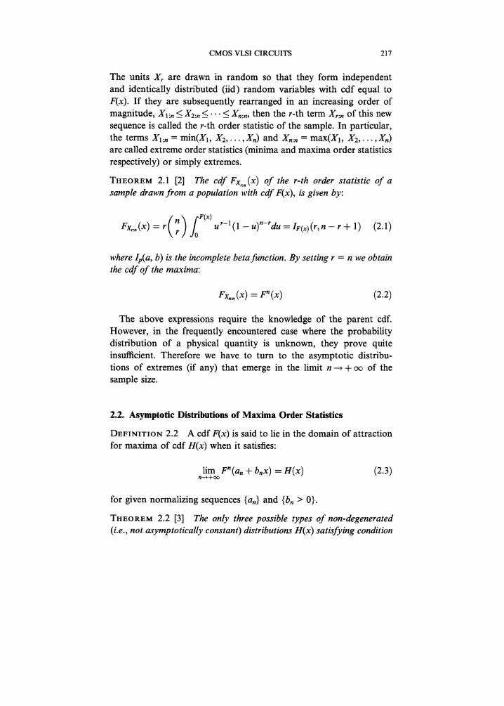
The units Xr are drawn in random so that they form independentand identically distributed (iid) random variables with cdf equal toF(x). If they are subsequently rearranged in an increasing order ofmagnitude, Xl:n < Xz:n <"" < Xn:n, then the r-th term Xr:n of this newsequence is called the r-th order statistic of the sample. In particular,the terms Xl:n min(X1, X2,... ,Xn) andare called extreme order statistics (minima and maxima order statisticsrespectively) or simply extremes.

THEOREM 2.1 [2] The cdf Fx,:.(x) of the r-th order statistic of asample drawn from a population with cdf F(x), is given by:

Fx,:,(x) r ur-l(1 u)n-rdu IF(x)(r,n- r + 1) (2.1)

where lp(a, b) is the incomplete betafunction. By setting r n we obtainthe cdf of the maxima:

Fx,:, (x) Fn(x) (2.2)

The above expressions require the knowledge of the parent cdf.However, in the frequently encountered case where the probabilitydistribution of a physical quantity is unknownl they prove quiteinsufficient. Therefore we have to turn to the asymptotic distribu-tions of extremes (if any) that emerge in the limit n + of thesample size.

2.2. Asymptotic Distributions of Maxima Order Statistics

DEINIIO 2.2 A cdf F(x) is said to lie in the domain of attractionfor maxima of cdf H(x) when it satisfies:

lim Fn(an + bnx) H(x) (2.3)

for given normalizing sequences {an} and {bn > 0}.

THEOREM 2.2 [3] The only three possible types of non-degenerated(i.e., not asymptotically constant) distributions H(x) satisfying condition


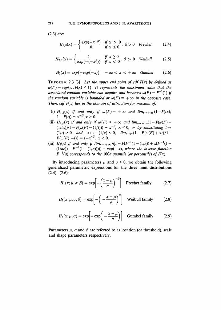
(2.3) are:

H1,/(x) ( exp(-x-)O /fx>0if x <_ 0 /3 > 0 Freehet (2.4)

/fx_>OH23(x) exp(-(-x)) if x < O’ 3 > 0 Weibull (2.5)

H3(x) exp(-exp(-x)) < x < + oo Gumbel (2.6)

THEOREM 2.3 [3] Let the upper end point of cdf F(x) be defined as

w(F) sup{x:F(x) < 1}. It represents the maximum value that theassociated random variable can acquire and becomes w(F) F-1(1) /fthe random variable is bounded or w(F)= + o in the opposite case.Then, cdf F(x) lies in the domain of attraction for maxima of’.

(i) H1,B(x) /f and only if w(F)= / oo and limt+o (1-F(tx)/1- F(t)) x-,x > O.

(ii) H2,a(x) /f and, only if w (F) < + oo and limt +(1 F(w(F)(1/tx))/1-F(w(F)-(1/t))) x-B, x < O, or by substituting t(I/t) > 0 and x -(I/x) < 0, limt-,o+(1 F(w(F) + xt)/1-F(w(F) -t)) (-x), x < O.

(iii) H3(x) /f and only if lim, + oo n[1 F(F- a(1 (1 In)) + x(F-l(1(1/ne)) F- 1(1 (1/n))))] exp(- x), where the inverse functionF-l(a) corresponds to the lOOa quantile (or percentile) of F(x).

By introducing parameters # and cr > 0, we obtain the followinggeneralized parametric expressions for the three limit distributions(2.4)-(2.6):

x -. #. Frechet family (2.7)/-/ (x; #, o’, ) expr

H2(x;#,a,/)= expl- ( x # Weibull family (2.8)

H3(x; #, a)= exp[-exp( Gumbel family (2.9)

Parameters #, a and are referred to as location (or threshold), scaleand shape parameters respectively.


2.3. Properties of Asymptotic Distributions

This section contains some important facts about the three afore-mentioned families of asymptotic distributions. Theorem 2.3 impliesthat a parent distribution with a finite upper end point (w(F) <cannot lie in a Frechet-type domain of attraction, whereas a distribu-tion with an infinite upper end point (w(F) + oe) cannot belong to aWeibull-type domain of attraction. However, these observationsare not enough to guarantee a Frechet or Weibull-type domain ofattraction for a particular distribution. In fact the Gumbel limitdistribution, even though it is not bounded by itself, asymptoticallymodels many parent distributions with either finite or infinite endpoints. The upper end point of the Weibull family (2.8) is equal to thelocation parameter #, while both Frechet and Gumbel families haveinfinite upper end points.The domain of attraction of a cdf F(x) is determined by the rate with

which its right tail approaches the value ofone as x w(F). Dependingon this rate we can distinguish between three families of distributions[4], namely the Cauchy-Pareto family, the Beta family (a special case ofwhich is the well-known uniform distribution) and the Exponentialfamily (which includes most of the common statistical distributionssuch as the Normal and Gamma ones). The Cauchy-Pareto family ischaracterized by an infinite upper end point and a very slow rate ofconvergence to one at its tail and is therefore asymptotically modeledby a Frechet limit distribution. The tail of a distribution of theExponential family converges to one at least as fast as that of theexponential distribution with cdf F(x)= 1-exp(-(x-a2)/a). Bothunbounded and bounded cdfs belong to this family and are all modeledby a Gumbel limit distribution at their extremes. Finally, members ofthe Beta family of distributions, which asymptotically approach theWeibull limit distribution, exhibit the faster (approximately linear)convergence towards one and are all bounded by finite upper limits.

2.4. Tail Equivalence

DEFINITION 2.3 TWO cdfs F(x) and G(x) are referred to as right tailequivalent if and only if

w(F)=w(G) and lim1-F(x)

xw(F) 1 G(x)1.


THEOREM 2.4 [5] Two right tail equivalent cdfs F(x) and G(x) belongto the same domain of attraction for maxima and have the samenormalizing sequences an and bn i.e.,

tim Fn(an + bnx) lira Gn(an + bnx) H(x).n--+oo n---+o

The practical implication of the above theorem when dealing withextreme value problems, is that a common cdf F(x) may be fitted to theright tail of an unknown cdf G(x) which is observed to follow the samelimit distribution as F(x). This will be the basis of the maximum powerestimation method proposed throughout this paper.

2.5. Probability Plots

The basic concept of a probability plot of a given parametric familyF(x; O) of distributions with vector parameter 0, is to modify therandom variable X and probability P axes scales in such way that theplot against X of any cdf belonging to that family becomes a straightline [6]. This allows one to decide whether or not a set of ordered datafollows a probability distribution drawn from that particular family.More specifically, if F(x; O) can be written as y F(x; O) h-l(ag(x)+ b), then the transformation g(x), h(y) changes F(x; O) into afamily of straight lines r/= a+ b.

Such a transformation can be applied to the parametric families(2.7)-(2.9) by taking logarithms twice:

log(- log(y)) =/3 log(x #) -/3 log cr

log(- log(y)) -/3 log(# x) +/3 log a

Frechet probability plotequation

(2.10)

Weibull probability plotequation

(2.11)

log(- log(y)) -xl _U Gumbel probability plot equation

(2.12)


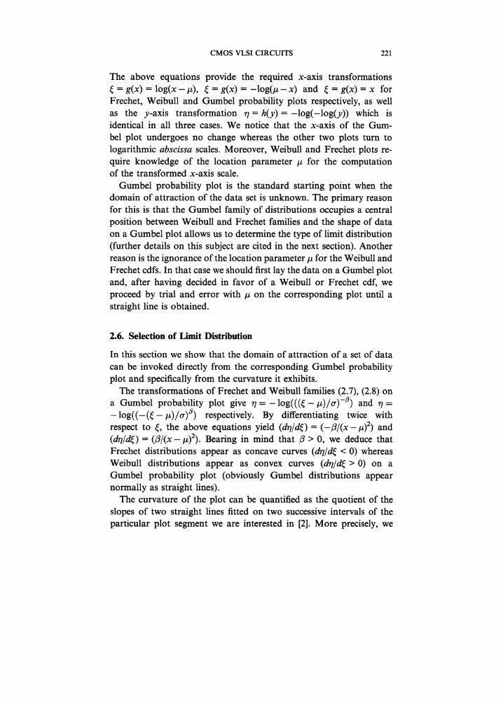
The above equations provide the required x-axis transformationsg(x) log(x- #), g(x) -log(#- x) and g(x) x for

Frechet, Weibull and Gumbel probability plots respectively, as wellas the y-axis transformation r/= h(y)=-log(-log(y)) which isidentical in all three cases. We notice that the x-axis of the Gum-bel plot undergoes no change whereas the other two plots turn tologarithmic abscissa scales. Moreover, Weibull and Frechet plots re-quire knowledge of the location parameter # for the computationof the transformed x-axis scale.Gumbel probability plot is the standard starting point when the

domain of attraction of the data set is unknown. The primary reasonfor this is that the Gumbel family of distributions occupies a centralposition between Weibull and Frechet families and the shape of dataon a Gumbel plot allows us to determine the type of limit distribution(further details on this subject are cited in the next section). Anotherreason is the ignorance of the location parameter # for the Weibull andFrechet cdfs. In that case we should first lay the data on a Gumbel plotand, after having decided in favor of a Weibull or Frechet cdf, weproceed by trial and error with # on the corresponding plot until astraight line is obtained.

2.6. Selection of Limit Distribution

In this section we show that the domain of attraction of a set of datacan be invoked directly from the corresponding Gumbel probabilityplot and specifically from the curvature it exhibits.The transformations of Frechet and Weibull families (2.7), (2.8) on

a Gumbel probability plot give r/=-log(((-#)/or)-) and-log((-(-#)/cr)a) respectively. By differentiating twice withrespect to , the above equations yield (d/d)= (-/(x-#)2) and(drl/d) (//(x-t)2). Beating in mind that > 0, we deduce thatFrechet distributions appear as concave curves (d/d < 0) whereasWeibull distributions appear as convex curves (d7/d > 0) on aGumbel probability plot (obviously Gumbel distributions appearnormally as straight lines).The curvature of the plot can be quantified as the quotient of the

slopes of two straight lines fitted on two successive intervals of theparticular plot segment we are interested in [2]. More precisely, we


compute the quantity S (S,,,2/Sn3,n,), where

is the slope of the least-squares straight line fit on the order statistics

Xk with index k between ni andIf the value of S, calculated on a Gumbel probability plot, is well

above 1 or well below 1, we may decide in favor of a Weibull orFrechet-type domain of attraction respectively. Significance levelsof this test are also provided in the literature [2], though not byanalytical calculation but from extensive Monte Carlo simulations(over 5000 units) that were applied on a Gumbel parent.

2.7. Parameter Estimation

The next step after determining the domain of attraction of a parentdistribution, is to estimate parameters #, g and (possibly)/ which arefound in expressions (2.7)-(2.9).

If the domain of attraction turns out to be of Gumbel-type, wemust first perform a least-squares straight line fit to the Gumbelprobability plot and then estimate parameters # and cr by match-ing the line equation coefficients to the ones in (2.12).

If the domain of attraction is of Weibull or Frechet-type, we mustcreate the corresponding probability plot for various values of # untilwe obtain the best straight line in terms of the minimum fit error. After# is determined, we may proceed with the estimation of parameters cr

and/3 by matching the line equation to (2.10) or (2.11), just as in theGumbel case. However, for the particular problem we are dealing


with, we do not need those parameters, since (as it will become clearin Section 3) we are only interested in the location parameter/z.

3. MAXIMUM POWER ESTIMATION PROCEDURE

3.1. Problem Formulation

The term "maximum power" refers to the worst-case instantaneouspower (or equivalently current) that is drawn from the supply bus.In order to render the estimation problem precise, we have to con-sider the sources of power dissipation in digital CMOS circuits,which are [8] Pswitching, Pshort-cireuit and Pleakage. The first two quan-tities are the dynamic components of total power since they onlyoccur at transitions between logic states, whereas the third one is thestatic component as it is a constant source of dissipation. Becauseof its static nature, leakage power may be regarded as an offsetto the total instantaneous power, while at the same time, it is twoto three orders of magnitude smaller than the other two components.It is therefore clear that the worst-case power conditions arise stric-tly on transition intervals and that any corresponding analysisshould be restricted inside a clock cycle which marks a transition be-tween two consecutive binary vectors. Because of this, maximum powerestimation is also referred to as cycle-accurate power estimation.

Within this context, estimation of maximum power is a fundamen-tally different problem than that of average power estimation. Theformer is related to the maximum value, among all possible vectorpairs, of the instantaneous power consumed within a clock cycle,whereas the latter involves the mean power of a sequence of inputpatterns applied over a large number of clock cycles that cover anextended period of time. From a statistical point of view, the prob-ability distribution of average power exhibits smoothing propertiesover time and approximates a normal (Gaussian) distribution asthe number of clock cycles tends to infinity. On the other hand,instantaneous power is considered within short periods of time andtherefore its probability distribution is completely undetermined. Inaddition, a normal distribution model may be suitable for the centerof the distribution but not for the tail which always follows an


asymptotic extreme value model. Consequently, conventional prob-abilistic and statistical techniques [9, 10], though have proved suc-cessful for average power estimation, are not adequate to handlemaximum power and a radically different approach should be adopt-ed which makes use of extreme value theory.

Instantaneous power dissipation in a CMOS circuit depends uponthe specific pair of binary vectors (Vl, v2) that define a transition on aparticular clock edge. If the number of primary inputs is n, then sucha vector consists of n bits and obviously the population of inputvector pairs contains 2n. 2n= 4n units. We will restrict our analysisto combinational circuits and furthermore, we will assume that allprimary inputs execute their transitions simultaneously on the sameclock edge. However, the generalization to a sequential circuit isstraightforward, if we expand the "previous" input vector vl toencompass the state bits (or outputs) of all sequential elements (flip-flops) of the circuit. In that case, if the number of state bits is m, thenthe input population will contain 2n+m. 2n 4n. 2" units. We shouldalso remark that the input population may not always include allpossible vector pairs but only selected ones that correspond to typicalcircuit operation or input switching activity (constrained problem).

3.2. Procedure Description

Since we have defined an input population of vector pairs, we mayregard the instantaneous power consumption of a particular cir-cuit as a random variable with a certain probability distribution. Therequired maximum power will then be represented by the upper endpoint w(F) of this distribution. The proposed method closely followsthe concepts presented in Section 2. However, in order to apply themwe must assume a continuous probability distribution of powerconsumption and an input population of infinite size. Both assump-tions are most frequently justified in practice for circuits of reason-able size with a moderate number of primary inputs (8 or more).A flow chart of the estimation procedure is depicted in Figure 1. The

main point is to acquire a number of distinct samples, form anadditional sample of maxima and graphically transfer it to a Gumbelprobability plot in order to determine the domain of attraction andultimately the upper end point of the probability distribution. The

power values

Drew Gumbelprobability plot andcalculate curvature

value S

Draw exponentialprobability plot for all

30 samples

Estimate paremetersand from

least.squares line fitfor all 30 samples

Estimate parameterlJfrom least-squares linefit Gumbel plot for

maxima

Estimate upper endpoint from equation

(3.4)

2.588Y

Drew Welbullprobability plot for thesample of maxima

Perform least-squaresstraight line fit and

;

function minimizationJ algorithm

Estimate upper endpoint the value oftomin’m’zeflterror

FIGURE Flow chart of the proposed method for maximum power estimation.


procedure begins with the generation of a number of vector pairsin random way or under certain constraints. This is equivalent torandom sampling out of the unconstrained or constrained popula-tion of input vector pairs. The circuit due for maximum power ana-lysis is entered in a transistor-level or gate-level simulator such asSPICE or PowerMill. Each generated vector pair is fed as input fortransient analysis to the simulator and the peak power during tran-sition time is recorded. The set of power values obtained for all gene-rated vector pairs forms one of the samples to be used hereafterand the procedure is repeated for the rest of them.The choice of sample size is critical at this point, in order to ensure

the validity of the asymptotic models for the minimum possiblenumber of units. Experiments performed on various parent distri-butions have shown that the rate of convergence to the corres-ponding domains of attraction is reasonably fast. Indeed, mostdistributions already approach their limit distribution as soon asthe sample reaches a size of about 30 to 50 units, depending on thetype of distribution, the problem size and the quality of the selectedunits. The worst case is encountered in the case of normal distribu-tion, which takes about 100 units to approach its Gumbel-type limitdistribution. Thus, the sample size is set to n 100. However onemay further improve the quality of the final estimate by increasingthe sample size. The choice of the number of samples, or equivalen-tly the size of the sample of maxima, is less critical and a total ofrn 30 is more than adequate in most cases. On the whole, thetotal number of units required to obtain an estimate of the maxi-mum power is 3000, which is significantly smaller (by a factor of 2Xto 10X) than the majority of the existing methods.The sample of maxima of power values is subsequently laid on a

Gumbel probability plot and the domain of attraction is determinedwith the aid of the curvature method presented in Section 2.6.According to Monte Carlo tests reported in [2], the critical value of thecurvature S for a sample size of 100 is S 2.588, with a significancelevel of 95%. The indices of the order statistics that define the inter-vals encountered in the calculation of S are chosen as nl 1, n.n3 m/2 and n4 m.Due to physical limitations, it is obvious that the probability

distribution of power consumption for a particular circuit is upperbounded (i.e., it has a finite upper end point) and therefore it can only


lie in the domain of attraction of Gumbel or Weibull families(Theorem 2.3). Consequently the proposed method has consideredboth types of asymptotic models.

If the limit distribution turns out to be of Gumbel-type, we mayinfer (due to the discussion in Section 2.3) that the parent distributionbelongs to the Exponential family regarding its rate of convergence toone as x w(F). The tail equivalence principle (Theorem 2.4) allowsus then to approximate the right tail of the unknown parent dis-tribution with a function of the form:

F(x)--al-exp( x-a a2), al>l (3.1)

If al is close to then F(x) is a probability distribution with the samerate of convergence to one (and consequently with the same Gumbel-type domain of attraction) as the standard exponential distribution,but which has a finite upper end point equal to:

w(F) F-l(1) a2 a log(al 1) (3.2)

Estimates of parameters a2 and a (location and scale respectively)may be derived with the same approach cited in Section 2.7 for theGumbel parameter estimation, i.e., by fitting a straight line on aprobability plot and by subsequently matching the coefficients ofthe line and plot equations. Care though has to be taken in that thetype of probability plot is now exponential and also that the sam-ple does not necessarily follow the distribution for which the plot isdesigned, which means that the fit should only include the right tailof the sample. A good choice for the number of points comprisingthe tail is 2v/-. Parameters a2 and a are estimated for all 30 samplesof power and mean values are taken out of them. The extra param-eter al in (3.2) cannot be estimated from the exponential probabilityplot since the latter is designed for the standard exponential distri-bution F(x) -exp(-(x- a2)/a). However, al is associated with theGumbel location parameter # of the sample of maxima, throughthe relation (see Appendix):

al= exp( #-a a2) +1 --nl (3.3)


For the estimation of parameter # we refer again to Section 2.7 andthe Gumbel probability plot of maxima that we have already created.When (3.3) is substituted in (3.2), we obtain the following estimateof the upper end point for the Gumbel case:

w(F)=a2-alog [exp (- # a2)_] (3.4)

The case of a Weibull limit distribution is considerably easier than theGumbel one, since the upper end point is equal to the locationparameter # which can be estimated as the value to give the beststraight line in terms of the minimum fit error on the Weibull plot(Section 2.7).To be more specific, we calculate the sum of squared errors be-

tween the data and the corresponding coordinates of the straight linefit as a function of #, and then employ a function minimizationalgorithm such as the Nelder-Mead simplex method [7].

4. EXPERIMENTAL RESULTS

Experiments have been conducted on two sets of distributionswhich are assumed to come close to the behavior of instantane-ous power consumption in VLSI circuits. Distributions that belongto the first set asymptotically follow the Gumbel model, whereasmembers of the second set are associated with the Weibull extrememodel. Each set embodies four distributions with range of values15.00-49.54mW, 15.00-222.69mW, 15.00-533.08 mW and 500.00-707.23 mW respectively. The difference between these two sets isobviously their speed of ascent from the lower end point towardsthe upper end point. Experimental results for the first and the secondset of distributions are shown in Tables I and II respectively. Bothtables display the average, maximum and minimum values of theestimated upper end point and the relative percentage error over100 runs of the procedure for each distribution. The intermediategraphs created for a single run of the estimation procedure appliedon the third distribution of both sets are depicted in Figures 2-4(Gumbel set) and Figures 5-7 (Weibull set).


TABLE Results for distributions with Gumbel-type domain of attraction

Actual upper Estimated value Relative error (%)endpoint Average Max Min Average Max Min

49.54 50.93 53.83 48.66 2.90 8.66 0.07222.69 229.07 244.05 219.03 2.95 9.59 0.11533.08 548.82 590.01 516.99 3.36 10.68 0.01707.23 716.17 737.33 700.79 1.32 4.26 0.01

TABLE II Results for distributions with Weibull-type domain of attraction

Actual upper Estimated value Relative error (%)end point Average Max Min Average Max Min

49.54 49.54 49.57 49.50 0.02 0.09 0222.69 222.67 222.93 222.35 0.03 0.15 0533.08 532.98 533.42 531.07 0.03 0.38 0707.23 707.21 707.50 706.76 0.01 0.07 0

50 100 150 200 250 300 350Data

FIGURE 2 Approximate probability distribution of Gumbel-type domain of attrac-tion and exponential fit on tail data.

Two important observations can be made by closer examinationof the above tables. The first one is that the method appears to bemuch more precise when dealing with distributions of Weibull-type


1.5

50 100 250

0.99

0.98

0,95

0.9

0.75

0.5

0.25

150 200 300 350Data

FIGURE 3 Exponential probability plot (with equation -log(1 -y) x/a- a2/a) andleast-squares straight line fit on tail data.

"*" 0.95

;.- 0.5

250 300 350 400 450 500Data

FIGURE 4 Gumbel probability plot of Gumbel-type domain of attraction and least-squares straight line fit.


, ....i.

..

o. ,.i....0.2 ’’

:i, ,

50 100 150 200 250 300 350 400 450 500Data

FIGURE 5 Approximate probability distribution of Weibull-type domain of attrac-tion.

10.99

0.98

3= 0.95

0.9

1.’/5

o...:oO

0-i

0.25

:- - 0,,

0.0

0.02i. ,I,-, I,. 0.01

505 510 515 520 525 530Data

FIGURE 6 Gumbel probability plot of Weibull-type domain of attraction.


0.98

. 0.9a- :’.

I :---:---: 0.75

.I -...:...:... 0,05

-i o.o50 10 1 5ao 55

Data

FIGURE 7 Weibull probability plot of Weibull-type domain of attraction and bestleast-squares straight line fit.

domain of attraction. This is not a direct result of our method butstems from the fact that, for random and equal-sized samples, a dis-tribution with a fast rate of ascent will exhibit more sample pointsbelonging to its right tail than a distribution with a slower rate ofascent (as is obvious from Figs. 2 and 5). The second observationis that estimates of the upper end point in the Gumbel case appearslightly biased towards larger values than the actual ones on average.This can be attributed to the fact that estimation of parameters a2and a of (3.1) is performed through a probability plot which isdesigned for the standard exponential distribution. However, thisdistribution has an infinite upper end point, which is a cause fora small positive bias on the estimated value of a finite one.

5. CONCLUSIONS

Fast and accurate estimation of maximum instantaneous powermay both allow to spot reliability problems early in the design phaseas well as to perform efficient design and optimization of the power


distribution network. A statistical approach based on extreme valuetheory has been proposed to address these issues. The method’sstrongest benefit is its speed, which is mainly due to the fact that asmall subset of input vectors captures all the necessary informationfor extreme value analysis. In addition, the simulative nature of themethod renders it a very attractive alternative solution, as its in-tegration within the design flow of digital CMOS VLSI circuits isstraightforward.

References[1] Qiu, Q., Wu, Q. and Pedram, M. (1998). "Maximum power estimation using the

limiting distributions of extreme order statistics", ACM/1EEE Design AutomationConference.

[2] Castillo, E. (1988). Extreme Value Theory in Engineering, Academic Press.[3] Galambos, J. (1987). The Asymptotic Theory ofExtreme Order Statistics 2nd edn.,

Krieger.[4] Reiss, R.-D. and Thomas, M. (1997). Statistical Analysis of Extreme Values,

Birkhauser Verlag.[5] Resnick, S. (1971). "Tail equivalence and its applications", J. Applied Probability,

$, 136-156.[6] Hahn, G. and Shapiro, S. (1994). Statistical Models in Engineering, Wiley.[7] Nelder, J. and Mead, R. (1965). "A simplex method for function minimization",

Computer J., 7, 308-313.[8] Weste, N. and Eshragian, K. (1993). Principles ofCMOS VLSI Design: A Systems

Perspective 2nd edn., Addison-Wesley.[9] Burch, R., Najm, F., Yang, P. and Trick, T., "A Monte Carlo approach for power

estimation", 1EEE Trans. VLS1 Systems, 1, 63-71, Mar., 1993.[10] Stamoulis, G. and Hajj, I. (1993). "Improved techniques for probabilistic

simulation including signal correlation effects", ACM/1EEE Design AutomationConference.

APPENDIX

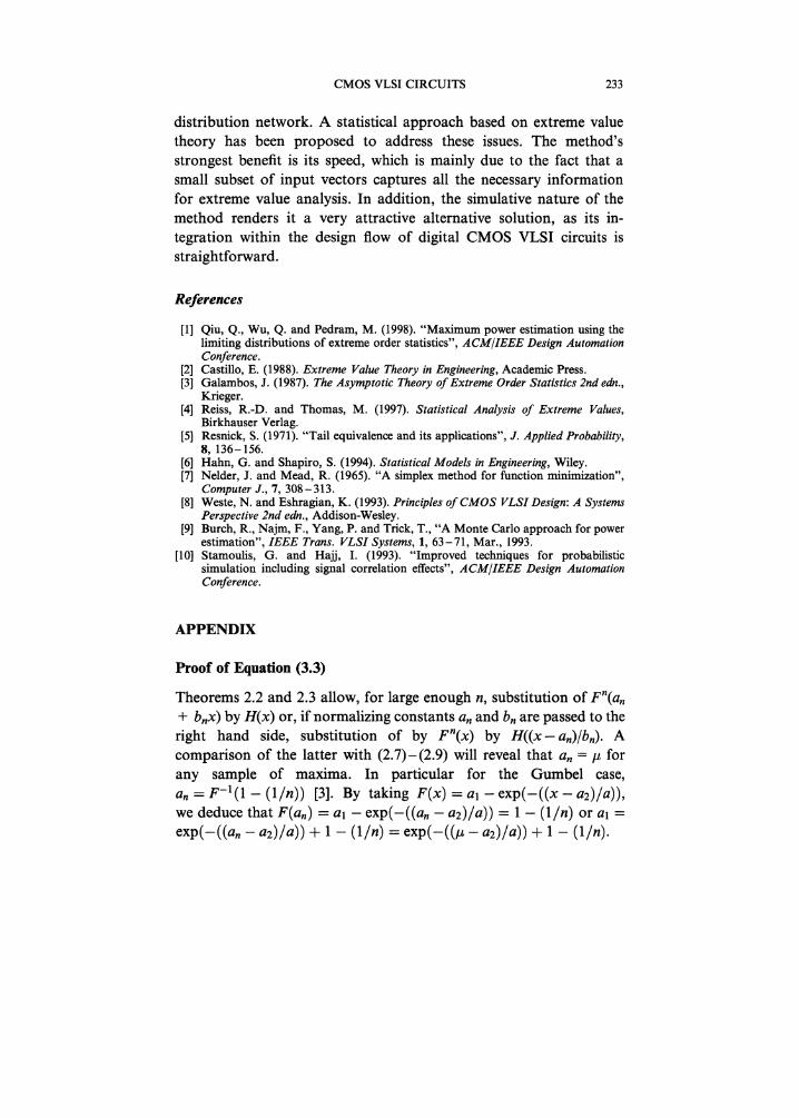
Proof of Equation (3.3)

Theorems 2.2 and 2.3 allow, for large enough n, substitution of Fn(an+ bnx) by H(x) or, if normalizing constants an and bn are passed to theright hand side, substitution of by Fn(x) by H((x-an)/bn). Acomparison of the latter with (2.7)-(2.9) will reveal that an # forany sample of maxima. In particular for the Gumbel case,an F-l(1 (l/n)) [3]. By taking F(x) al exp(-((x a2)/a)),we deduce that F(an) al exp(-((an a2)/a)) 1 (l/n) or al

exp(-((an a2)/a)) + 1 (l/n) exp(-((# a2)/a)) + 1 (l/n).

International Journal of

AerospaceEngineeringHindawi Publishing Corporationhttp://www.hindawi.com Volume 2010

RoboticsJournal of

Hindawi Publishing Corporationhttp://www.hindawi.com Volume 2014


Active and Passive Electronic Components

Control Scienceand Engineering

Journal of



RotatingMachinery


Hindawi Publishing Corporation http://www.hindawi.com

Journal ofEngineeringVolume 2014

Submit your manuscripts athttp://www.hindawi.com

VLSI Design



Shock and Vibration


Civil EngineeringAdvances in

Acoustics and VibrationAdvances in



Electrical and Computer Engineering

Journal of

Advances inOptoElectronics

Hindawi Publishing Corporation http://www.hindawi.com

Volume 2014

The Scientific World JournalHindawi Publishing Corporation http://www.hindawi.com Volume 2014

SensorsJournal of


Modelling & Simulation in EngineeringHindawi Publishing Corporation http://www.hindawi.com Volume 2014


Chemical EngineeringInternational Journal of Antennas and

Propagation




Navigation and Observation



DistributedSensor Networks


a statistical method for maximum power estimation …

Documents