statistical extended-range forecast of winter surface air...

Quarterly Journal of the Royal Meteorological Society Q. J. R. Meteorol. Soc. 143: 1528–1538, April 2017 A DOI:10.1002/qj.3023

Statistical extended-range forecast of winter surface air temperatureand extremely cold days over China

Zhiwei Zhua,b* and Tim Lia,b

aKey Laboratory of Meteorological Disaster, Ministry of Education (KLME)/Joint International Research Laboratory of Climate andEnvironment Change (ILCEC)/Collaborative Innovation Center on Forecast and Evaluation of Meteorological Disasters (CIC-FEMD),

Nanjing University of Information Science and Technology, Nanjing, ChinabDepartment of Atmospheric Sciences, International Pacific Research Center, University of Hawaii, Honolulu, HI, USA

*Correspondence to: Z. Zhu, IPRC, SOEST, University of Hawaii, 1680 East West Road, POST Bldg. 401, Honolulu, HI 96822, USA.E-mail: [email protected]

An extremely cold day (ECD) in boreal winter over China is often accompanied by freezingrainfall or snow, leading to power outages, paralysed traffic and damaged ecosystems.Extended-range (5–30 days lead) forecast of Chinese winter surface air temperature (SAT)and ECD has become a critical demand nationwide. In the present study, based on trainingdata during 1960/1961–1999/2000, a statistical spatial–temporal projection model (STPM)is conducted to carry out an independent extended-range forecast of winter SAT and ECDover China.

For the independent forecast period (2000/2001–2012/2013), STPM is able to capture theempirical orthogonal function (EOF)-filtered 10–80 days SAT anomaly at all 5–30 days leadtimes. Verification against the observed 10–80 days SAT anomaly shows that significanttemporal correlation coefficient skill persists to 25–30 days lead times over most parts ofChina, except for northeastern China and the Tibetan Plateau where useful skill is upto a 15 days lead time. Significant pattern correlation coefficients between forecasted andthe EOF-filtered/observed 10–80 days SAT anomaly account for over 63%/59% of totalforecasts for all 5–30 days lead times.

The forecast local ECD is determined based on reconstructed SAT by adding the lowerfrequency (longer than 80 days) climatological SAT to the forecast 10–80 days SAT anomaly.Except for southeastern China and the Tibetan Plateau, STPM can hit above 30% of localECDs over most parts of China at least 15 days in advance.

Key Words: spatial–temporal projection model; winter surface air temperature over China; extremely cold days;extended-range forecast

Received 10 October 2016; Revised 9 January 2017; Accepted 21 February 2017; Published online in Wiley Online Library21 April 2017

1. Introduction

China stretches across a vast area covering the cold, temperateand tropical zones. Because of the prevailing East Asian wintermonsoon, low-temperature air mass from Siberia is transported tolower latitudes, influencing the whole of China (Ding, 1990; Gonget al., 2001; Wang et al., 2010). During boreal winter, extremelycold temperatures and blizzards are frequent in northern China,whilst freezing rain and snowstorms tend to occur over southernChina owing to the confluence of cold air from high latitudesand warm moisture from tropical oceans. In the context of Arcticwarming, because of the enhanced meridional transportation ofcold air from the polar regions (Jiang et al., 2012; Liu et al., 2012;Ma et al., 2012; Kim et al., 2014; Kug et al., 2015), increasing harshcold winters have occurred in the past few years over East Asia. Forinstance, a series of winter storm events with heavy snow, ice andcold temperatures in the 2007/2008 winter affected large portions

of southern and central China, causing extensive infrastructuredamage, transportation disruptions and more than one hundredfatalities (Zhou et al., 2009; Wu et al., 2011; Li and Wu, 2012).More recently in the 2015/2016 winter, the temperature droppedto −47 ◦c over Inner Mongolia, and plunged to around 3–4 ◦cover Hong Kong (lowest temperature recorded in 59 years) andTaiwan (coldest recorded in 44 years). Given the foreseeablegreater frequency of extremely cold days (ECD) in the nearfuture, accurate subseasonal to seasonal forecasting of wintersurface air temperature (SAT) and ECD has become a nationwidepublic demand of the utmost urgency.

Considerable efforts have been devoted to seasonal predictionof winter SAT and ECD over China (Lee et al., 2013). It is suggestedthat about 50% of the total variance of the number of ECDis predictable by a physics-based empirical seasonal predictionmodel (Luo and Wang, 2016). However, studies on subseasonalor extended-range statistical forecasting of SAT and ECD remains

c© 2017 Royal Meteorological Society

http://orcid.org/0000-0002-4885-1299

Extended-range Forecast of Winter Surface Temperature over China 1529

a big challenge. Recently, we developed several spatial–temporalprojection models (STPMs) in which the extended single valuedecomposition was used to extract the information of temporallyvarying coupled predictor–predictand modes. These STPMswere successfully applied to extended-range (5–30 days lead)forecasts over both the Tropics and extratropics. For example,tropical convection patterns associated with the Madden–JulianOscillation (MJO) were predicted reasonably well at a lead time of25–30 days (Zhu et al., 2015); the occurrence of clustering tropicalcyclones over the western North Pacific were captured at a 15 dayslead time (Zhu et al., 2016); useful forecast skill of subseasonalsummer rainfall was achieved at a lead time of 20 days over mostparts of China (Zhu and Li, 2017a); and the onset date of theSouth China Sea monsoon was successfully forecasted (Zhu andLi, 2017b). In summary, STPM presents superior skills comparedto previous statistical models.

Given the satisfactory performance of the STPM over bothTropics and extratropics, it will be of benefit to apply STPM toforecasting winter SAT and ECD over China. Therefore, the maingoal of this article is to construct STPM and to assess forecast skillsof winter SAT and ECD over China. Following this introduction,section 2 introduces the data, method and the detail of STPM.In section 3, the predictability sources of winter SAT over Chinaand the projection domains for STPM are illustrated. The STPMforecast skill of winter SAT and ECD are presented in section 4.The last section provides conclusions and discussion.

2. Data, method and statistical model

2.1. Data

A homogenized minimum daily air temperature dataset isderived from the 753 stations in mainland China that are runby the China Meteorological Administration. The atmosphericcirculation variables are from National Centers for EnvironmentalPrediction and National Center for Atmospheric Researchreanalysis I (Kalnay et al., 1996). They have a horizontal resolutionby 2.5◦ × 2.5◦ (longitude × latitude). To focus on large-scalecirculation, the original datasets are interpolated into a 5◦ × 5◦resolution. A 5 days mean is first applied to all the datasets toform pentad data. Note that 29 February in a leap year is omitted,therefore there are always 73 pentads for each year. The datasetscover the period from 1960 to 2013. The winter season in thepresent study denotes the extended boreal winter (i.e. November,December, January, February, March and April) from pentad 62to pentad 24 of the next year.

2.2. Extraction of intraseasonal oscillation (ISO) signal

Figure 1 shows the fractional variance of the 10–80 days SATto the total pentad SAT. The largest fractional variance locatesover southern China, whereas northeast and western China hasa relatively smaller fractional variance. Nevertheless, as shownin Figure 1, 10–80 days SAT explains more than 70% of thetotal variance of SAT over most parts of China during borealwinter. The present study focuses on the 10–80 days band ofintraseasonal SAT. To avoid the tapering problem of a regularband-pass filter, an ‘unconventional filtering’ method is applied toextract the intraseasonal signal. This method has been employedin many previous studies to reliably and efficiently extract theintraseasonal signal (Hsu et al., 2015; Zhu et al., 2016; Zhu andLi, 2017a, 2017b). It has three steps to extract the 10–80 dayssignal: first, the climatological annual cycle is removed from theoriginal pentad-mean data by subtracting a climatological 18-pentad (90 days) low-pass filtered component; second, the last8-pentad (i.e. from day −40 to 0) running mean is removedfrom the anomalous field above, and therefore the low-frequencysignal that is longer than 16 pentads (80 days) is subtracted; third,because it is already in pentad-mean (i.e. from day −5 to 0), thesynoptic-scale signal (shorter than 10 days) is removed. By doing

55°N

0.95

0.9

0.85

0.8

0.75

0.7

50°N

45°N

40°N

35°N

30°N

25°N

20°N

15°N80°E 90°E 100°E 110°E 120°E 130°E

Figure 1. The fractional variance of intraseasonal (10–80 days) filtered SATvariability to the total SAT variability during the winter season (contour lines areat 0.05 intervals). [Colour figure can be viewed at wileyonlinelibrary.com].

so, the 10–80 days ISO signal is eventually extracted. Because nofuture data after the current date (day 0) is used, we can apply this‘unconventional filtering’ method to the real-time operationalforecast.

The ECD is defined in a similar way to previous studies (Joneset al., 1999; Li et al., 2016). For a given station, a local ECD isdefined if pentad-mean minimum air temperature is below the5th percentile threshold of a set of pentad records, including thoseobserved records on the same pentad and the neighbouring pentadfor all years in the training period (1960/1961 to 1999/2000).

2.3. Model specific

In the present study, the data from 1960/1961 to 1999/2000(40 years) are used for the training model, whereas the data from2000/2001 to 2012/2013 (13 years) are employed to assess themodel’s performance for an independent forecast. Six pentadprevious predictors and six pentad succeeding predictands areconcatenated to aim at 5–30 days (5, 10, 15, 20, 25 and 30 days,respectively) lead time forecasts at once. For example, thepredictors at pentad 62–67, pentad 63–68 . . . and pentad 67–72are used to forecast the predictand at pentad 68–73, pentad 69–1. . . and pentad 73–5 at each forecast time (at pentad 67, 68 . . .

72, respectively).Following our previous studies (Zhu et al., 2015; Zhu and

Li, 2017a), STPM is based on the extended singularity valuedecomposition (E-SVD). Since the SVD is able to extract thecoupled modes of two fields (Bretherton et al., 1992), the STPMbased on E-SVD could capture the temporally varying coupledmodes of the previous predictor and the following predictand. Asexpressed by Eqs (1) and (2), during the 40 years training period(1960/1961–1999/2000), the large-scale predictor (predictand)involves a data matrix X (Y) with t dimension points in time andi1 × j1 × 6 (i2 × j2 × 6) points in space, where 6 is the numberof preceding (succeeding) pentads corresponding to the currentforecast time point.

X(t, i1 × j1 × 6) ≈K∑

k=1

Vk(i1 × j1 × 6)vk(t), (1)

Y(t, i2×j2 × 6) ≈K∑

k=1

Uk(i2 × j2 × 6)uk(t). (2)

K, which equals 6 in the present study, is the total numberof E-SVD coupled modes that are derived during the training

c© 2017 Royal Meteorological Society Q. J. R. Meteorol. Soc. 143: 1528–1538 (2017)

wileyonlinelibrary.com

1530 Z. Zhu and T. Li

55°N

(a) (b) (c) (d)EOF1 47% EOF2 13% EOF3 Var6%

50°N

45°N

40°N

35°N

30°N

25°N

20°N

15°N

80°E 90°E 100°E 110°E 120°E 130°E 80°E 90°E 100°E 110°E 120°E 130°E 80°E 90°E 100°E 110°E 120°E 130°E 1 2 3 4 5 6 7 8 9 10

55°N

50°N

45°N

40°N

35°N

30°N

25°N

20°N

15°N

55°N 60

50

40

30

20

10

0

50°N

45°N

40°N

35°N

30°N

25°N

20°N

15°N

Figure 2. (a–c) The first three leading EOF modes of 10–80 days SAT, and (d) the fractional variance (line, unit: %) explained by the first ten EOF modes and theirerror (error bar). [Colour figure can be viewed at wileyonlinelibrary.com].

period. To avoid overfitting, only the persistent and useful modesduring the training period can be used to produce an independentforecast. These persistent modes are retained through the cross-validation (leaving 1 year out) procedure. The cross-validationprocedure involves the following three steps: (i) leaving out 1 yearof data (i.e. 25 pentads) and conducting the E-SVD analysisusing the remaining 39 years of training data; (ii) projecting the1 year left-out predictor and predictand onto the correspondingpredictor–predictand E-SVD modes that are derived from theremaining years, yielding a pair of 1 year’s projected expansioncoefficients (two time series of 25 pentads) for each of theK E-SVD modes; (iii) repeating step (i) and (ii) 39 timesby leaving out different 1 year data, combining the projectedexpansion coefficients for the total 40 years (25 × 40 pentads)for each coupled mode, and retaining m coupled modes withsignificant correlation coefficients (passing the 99% confidencelevel) between the pair of projected expansion coefficients.

During the independent forecast period (from time point tf),the reproduced expansion coefficient (vm) can be obtained byprojecting the real-time predictor field (X) onto the retainedm modes of predictor (Vm), as expressed by Eq. (3). Andfinally, owing to the high correlation coefficient between the twoexpansion coefficients, as indicated by Eq. (4), the independentforecasting of predictand (Y) could be made through simplymultiplying the reproduced expansion coefficient of predictors(vm) by the corresponding retained modes of predictand (Um).

vm(tf ) =i1×j1×6∑

k=1

X(tf , i1 × j1 × 6)×Vm(i1 × j1 × 6), (3)

Y(tf , i1 × j1 × 6) ≈M∑

m=1

Um(i1 × j1 × 6)·vm(tf ). (4)

The air temperature at 850 hPa (a850), temperature advectionat 850 hPa (advc) and sea-level pressure (slpa) are used aspotential predictors. Besides, vertical motion at 500 hPa (w500),geopotential heights at 200 hPa (h200) and relatively humidityat 700 hPa (rhum) are employed as potential predictors. Eachprincipal component (PC) of empirical orthogonal function(EOF) of Chinese SAT itself is selected as the potential predictoras well. An arithmetic mean is applied to make the ensembleforecast product for these seven STPM outputs.

The forecast temporally varying SAT pattern over Chinacan be reconstructed by the forecasted PCs and the observedEOF patterns. Five metrics are employed to evaluate the STPMperformance. The temporal correlation coefficient (TCC), theroot-mean-square error (RMSE), and the pattern correlationcoefficient (PCC) are used to evaluate the forecast of SAT

anomaly, whereas the hit rate and threat score are used forECD. Note that useful TCC skill involves an issue of theeffective degrees of freedom, thus we introduce a methodproposed by Bretherton et al. (1999) to estimate the effectivesample size (Ne) and the significance of TCC. The Ne formulais Ne = N (1 − r12)/(1 + r12), where r1 is the one-pentad lagautocorrelation and N is the original sample size (325, 25 pentadsper year over 13 years) for the independent forecast period of2000/2001–2012/2013. The one-pentad lag autocorrelation (r1)is around 0.13 for each PC; therefore the effective sample size isaround 310. Based on the effective sample size, TCC exceeding0.15 could be considered as a useful TCC skill (significant at the99% confidence level).

3. Predictability sources

Because China has a vast territory, precursors of winter SATover China are complex. To better seek the predictability sources,we first unravel the spatio-temporal characteristic of winter SATover China. Figure 2 shows the first three leading modes ofEOF analysis and the variance percentage explained by the firstten leading PCs. The spatial patterns of the first three leadingEOF modes for 10–80 days winter SAT over China presenta monopole, a dipole and a tripole pattern, respectively. Themonopole pattern of the first EOF (Figure 2(a)) has maximumloadings over eastern China. Relatively smaller loading appearsover the Tibetan Plateau, southwestern China, northwestern andnortheastern China probably owing to the high elevation ofthese regions. This mode accounts for 47% of the total varianceof 10–80 days SAT. The second EOF (Figure 2(b)) primarilyshows a meridional seesaw pattern. Positive loadings appear oversouthern and central western China, whereas negative loadingsare basically over northern China but with the exception ofwedge-shaped negative loadings over the middle reaches of theYangtze River basin. The third EOF mode basically presentsa zonal tripole pattern (Figure 2(c)) with negative loadingsin central and northwestern China but positive loadings oversoutheastern/northeastern (east of 115◦E) and southwesternChina. The second and third modes explain 13% and 6% ofthe total variance, respectively. As shown in Figure 2(d), the firstthree leading modes (accounting for 66% of the total 10–80 daysSAT variances) are highly independent and distinguished fromthe higher modes according to North et al. (1982).

Since the three leading modes already account for 66% ofthe total SAT variances and the higher modes are nothing butnoise, useful forecasts are achievable if the three leading EOFPCs can be reproduced reasonably well. The temporally varyingSAT pattern can be reconstructed through multiplying threeleading patterns of EOF by their corresponding PCs. Hereafterthe reconstructed SAT by the three leading EOF modes is called




75°N

60°N

45°N

30°N

15°N

EQ

15°S

30°S40°E 80°E 120°E 160°E160°W120°W 80°W 40°W 40°E 80°E 120°E 160°E160°W120°W 80°W 40°W 40°E 80°E 120°E 160°E160°W120°W 80°W 40°W

75°N

60°N

45°N

30°N

15°N

EQ

15°S

30°S

75°N

60°N

45°N

30°N

15°N

EQ

15°S

30°S

75°N

60°N

45°N

30°N

15°N

EQ

15°S


75°N

60°N

45°N

30°N

15°N

EQ

15°S

30°S

75°N

60°N

45°N

30°N

15°N

EQ

15°S

30°S

75°N

60°N

45°N

30°N

15°N

EQ

15°S


75°N

60°N

45°N

30°N

15°N

EQ

15°S

30°S

75°N

60°N

45°N

30°N

15°N

EQ

15°S

30°S

75°N

60°N

45°N

30°N

15°N

EQ

15°S


75°N

60°N

45°N

30°N

15°N

EQ

15°S

30°S

75°N

60°N

45°N

30°N

15°N

EQ

15°S

30°S

75°N

60°N

45°N

30°N

15°N

EQ

15°S


75°N

60°N

45°N

30°N

15°N

EQ

15°S

30°S

75°N

60°N

45°N

30°N

15°N

EQ

15°S

30°S

75°N

60°N

45°N

30°N

15°N

EQ

15°S


75°N

60°N

45°N

30°N

15°N

EQ

15°S

30°S

75°N

60°N

45°N

30°N

15°N

EQ

15°S

30°S

75°N

60°N

45°N

30°N

15°N

EQ

15°S


75°N

60°N

45°N

30°N

15°N

EQ

15°S

30°S

75°N

60°N

45°N

30°N

15°N

EQ

15°S

30°S

75°N

60°N

45°N

30°N

15°N

EQ

15°S

30°S

pc1_rhum

lead 5d lead 5d lead 5d








pc1_slpa pc1_w500

pc1_a850 pc1_advc pc1_h200

40°E 80°E 120°E 160°E160°W120°W 80°W 40°W 40°E 80°E 120°E 160°E160°W120°W 80°W 40°W 40°E 80°E 120°E 160°E160°W120°W 80°W 40°W

75°N

60°N

45°N

30°N

15°N

EQ

15°S

30°S

75°N

60°N

45°N

30°N

15°N

EQ

15°S

30°S

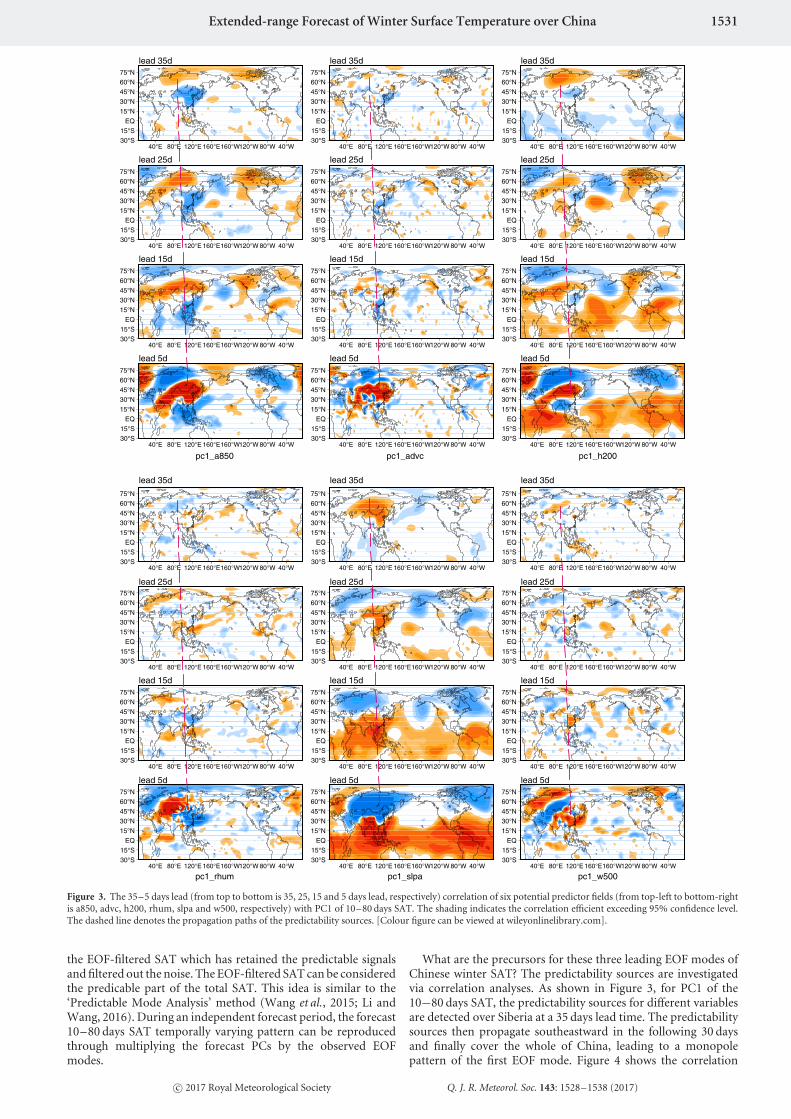
Figure 3. The 35–5 days lead (from top to bottom is 35, 25, 15 and 5 days lead, respectively) correlation of six potential predictor fields (from top-left to bottom-rightis a850, advc, h200, rhum, slpa and w500, respectively) with PC1 of 10–80 days SAT. The shading indicates the correlation efficient exceeding 95% confidence level.The dashed line denotes the propagation paths of the predictability sources. [Colour figure can be viewed at wileyonlinelibrary.com].

the EOF-filtered SAT which has retained the predictable signalsand filtered out the noise. The EOF-filtered SAT can be consideredthe predicable part of the total SAT. This idea is similar to the‘Predictable Mode Analysis’ method (Wang et al., 2015; Li andWang, 2016). During an independent forecast period, the forecast10–80 days SAT temporally varying pattern can be reproducedthrough multiplying the forecast PCs by the observed EOFmodes.

What are the precursors for these three leading EOF modes ofChinese winter SAT? The predictability sources are investigatedvia correlation analyses. As shown in Figure 3, for PC1 of the10−80 days SAT, the predictability sources for different variablesare detected over Siberia at a 35 days lead time. The predictabilitysources then propagate southeastward in the following 30 daysand finally cover the whole of China, leading to a monopolepattern of the first EOF mode. Figure 4 shows the correlation




75°N

60°N

45°N

30°N

15°N

EQ

15°S

30°S

75°N

60°N

45°N

30°N

15°N

EQ

15°S

30°S

75°N

60°N

45°N

30°N

15°N

EQ

15°S

30°S40°E 80°E 120°E 160°E160°W120°W 80°W 40°W 40°E 80°E 120°E 160°E160°W120°W 80°W 40°W 40° E 80°E 120°E 160°E160°W120°W 80°W 40°W

75°N

60°N

45°N

30°N

15°N

EQ

15°S

30°S

75°N

60°N

45°N

30°N

15°N

EQ

15°S

30°S

75°N

60°N

45°N

30°N

15°N

EQ

15°S


75°N

60°N

45°N

30°N

15°N

EQ

15°S

30°S

75°N

60°N

45°N

30°N

15°N

EQ

15°S

30°S

75°N

60°N

45°N

30°N

15°N

EQ

15°S


75°N

60°N

45°N

30°N

15°N

EQ

15°S

30°S

75°N

60°N

45°N

30°N

15°N

EQ

15°S

30°S

75°N

60°N

45°N

30°N

15°N

EQ

15°S


75°N

60°N

45°N

30°N

15°N

EQ

15°S

30°S

75°N

60°N

45°N

30°N

15°N

EQ

15°S

30°S

75°N

60°N

45°N

30°N

15°N

EQ

15°S


75°N

60°N

45°N

30°N

15°N

EQ

15°S

30°S

75°N

60°N

45°N

30°N

15°N

EQ

15°S

30°S

75°N

60°N

45°N

30°N

15°N

EQ

15°S


75°N

60°N

45°N

30°N

15°N

EQ

15°S

30°S

75°N

60°N

45°N

30°N

15°N

EQ

15°S

30°S

75°N

60°N

45°N

30°N

15°N

EQ

15°S


75°N

60°N

45°N

30°N

15°N

EQ

15°S

30°S

75°N

60°N

45°N

30°N

15°N

EQ

15°S

30°S

75°N

60°N

45°N

30°N

15°N

EQ

15°S


pc2_rhum pc2_slpa pc2_w500










Figure 4. Same as in Figure 3 but with PC2. [Colour figure can be viewed at wileyonlinelibrary.com].

between the PC2 and previous 35 to 5 days lead predictor fields.At a 35 days lead time, the predictability sources appear withopposite signs centred on the Barents Sea and northeastern Asia,respectively. Previous studies have revealed the mechanisms forthe formation of this dipole predictability source signal overthe Barents Sea and northeastern Asia. Because the changes ofsea ice over the Barents Sea is most pronounced compared toelsewhere in the polar regions, abnormal turbulent heat fluxesover the Barents Sea induced by the sea-ice reduction can initiate

a remote atmospheric response by triggering stationary Rossbywaves (Honda et al., 2009). The stationary Rossby waves showsopposite signs between the Barents Sea and northeast Asia/easternEurope. Another physical explanation (Inoue et al., 2012) for thedipole signal is that the change of Barents Sea ice can alterthe meridional location of the wintertime cyclone track andcause the cold/warm anomalous temperature advection over eastSiberia, leading to the dipole pattern over the Barents Sea andnortheast Asia. As shown in Figure 4, the two anomaly centres




75°N

60°N

45°N

30°N

15°N

EQ

15°S

30°S40°E 80°E 120°E 160°E160°W120°W 80°W 40°W

75°N

60°N

45°N

30°N

15°N

EQ

15°S

30°S40°E 80°E 120°E 160°E160°W120°W 80°W 40°W

75°N

60°N

45°N

30°N

15°N

EQ

15°S

30°S40°E 80°E 120°E 160°E160°W120°W 80°W 40°W

75°N

60°N

45°N

30°N

15°N

EQ

15°S

30°S40°E 80°E 120°E 160°E160°W120°W 80°W 40°W

75°N

60°N

45°N

30°N

15°N

EQ

15°S

30°S40°E 80°E 120°E 160°E160°W120°W 80°W 40°W

75°N

60°N

45°N

30°N

15°N

EQ

15°S

30°S40°E 80°E 120°E 160°E160°W120°W 80°W 40°W

75°N

60°N

45°N

30°N

15°N

EQ

15°S

30°S40°E 80°E 120°E 160°E160°W120°W 80°W 40°W

75°N

60°N

45°N

30°N

15°N

EQ

15°S

30°S40°E 80°E 120°E 160°E160°W120°W 80°W 40°W

75°N

60°N

45°N

30°N

15°N

EQ

15°S

30°S40°E 80°E 120°E 160°E160°W120°W 80°W 40°W

75°N

60°N

45°N

30°N

15°N

EQ

15°S

30°S40°E 80°E 120°E 160°E160°W120°W 80°W 40°W

75°N

60°N

45°N

30°N

15°N

EQ

15°S

30°S40°E 80°E 120°E 160°E160°W120°W 80°W 40°W

75°N

60°N

45°N

30°N

15°N

EQ

15°S

30°S40°E 80°E 120°E 160°E160°W120°W 80°W 40°W

75°N

60°N

45°N

30°N

15°N

EQ

15°S

30°S40°E 80°E 120°E 160°E160°W120°W 80°W 40°W

75°N

60°N

45°N

30°N

15°N

EQ

15°S

30°S40°E 80°E 120°E 160°E160°W120°W 80°W 40°W

75°N

60°N

45°N

30°N

15°N

EQ

15°S

30°S40°E 80°E 120°E 160°E160°W120°W 80°W 40°W

75°N

60°N

45°N

30°N

15°N

EQ

15°S

30°S40°E 80°E 120°E 160°E160°W120°W 80°W 40°W

75°N

60°N

45°N

30°N

15°N

EQ

15°S

30°S40°E 80°E 120°E 160°E160°W120°W 80°W 40°W

75°N

60°N

45°N

30°N

15°N

EQ

15°S

30°S40°E 80°E 120°E 160°E160°W120°W 80°W 40°W

75°N

60°N

45°N

30°N

15°N

EQ

15°S

30°S40°E 80°E 120°E 160°E160°W120°W 80°W 40°W

75°N

60°N

45°N

30°N

15°N

EQ

15°S

30°S40°E 80°E 120°E 160°E160°W120°W 80°W 40°W

75°N

60°N

45°N

30°N

15°N

EQ

15°S

30°S40°E 80°E 120°E 160°E160°W120°W 80°W 40°W

75°N

60°N

45°N

30°N

15°N

EQ

15°S

30°S40°E 80°E 120°E 160°E160°W120°W 80°W 40°W

75°N

60°N

45°N

30°N

15°N

EQ

15°S

30°S40°E 80°E 120°E 160°E160°W120°W 80°W 40°W

75°N

60°N

45°N

30°N

15°N

EQ

15°S

30°S40°E 80°E 120°E 160°E160°W120°W 80°W 40°W









pc3_rhum pc3_slpa pc3_w500


Figure 5. Same as Figure 3 but with PC3. [Colour figure can be viewed at wileyonlinelibrary.com].

over the Barents Sea and northeastern Asia then respectivelypropagate southeastward and southward in the following 30 days,and together arrive in northern and southern China, resultingin a dipole pattern of SAT, which corresponds to the secondEOF pattern. As to PC3 (Figure 5), the predictability sources aredetected at a 35 days lead time over northern Europe. They thenpropagate southeastward and reach China. At a 5 days lead time,a wave-number-4 Rossby wave train along 40◦N is formed. Thezonal wave train contributes to a tripole pattern over East Asia,which is consistent with the third EOF mode of Chinese SAT.

Once the predictability sources are detected, the projectiondomain for STPM can be determined. Our principle to choosethe projection domain is that the projection domain cannotbe too large (otherwise noise will be included when extractingthe coupled SVD modes), nor too small (otherwise some usefulsignals might be lost). Note that because the Arctic is the sourceof the cold air over East Asia, the origin of three leading modesof winter SAT over China can all be traced back upstream tothe polar regions and high latitudes of the Eurasian continent asshown in Figures 3–5. Therefore, for simplicity, the projection




Table 1. Temporal correlation coefficients and root-mean-square error (inbrackets) skills for each PC.

5 dayslead

10 dayslead

15 dayslead

20 dayslead

25 dayslead

30 dayslead

PC1 0.70 (0.72) 0.45 (0.97) 0.38 (1.04) 0.38 (1.05) 0.34 (1.05) 0.30 (1.07)PC2 0.58 (0.91) 0.37 (1.12) 0.33 (1.15) 0.31 (1.17) 0.29 (1.15) 0.26 (1.15)PC3 0.53 (0.87) 0.30 (1.04) 0.21 (1.09) 0.15 (1.09) 0.17 (1.06) 0.28 (1.02)

domains of STPM for the first three leading PCs are all selectedas 40◦E–140◦E, 15◦N–75◦N.

4. Forecast skills

Based on the selected projection domains, STPMs are conductedto forecast SAT for the period 2000/2001–2012/2013. Given thatthe direct forecast product of STPM is the three leading PCsof SAT, the forecast skills for each PC are first assessed. The

55°N5 days lead 0.65 10 days lead 0.42 15 days lead 0.35

20 days lead 0.34 25 days lead 0.31 30 days lead 0.30

5 days lead

TCC distribution against observed SAT

TCC distribution against EOF – filtered SAT

0.53 10 days lead 0.34 15 days lead 0.29

20 days lead 0.28 25 days lead 0.25 30 days lead 0.24

50°N

45°N

40°N

35°N

30°N

25°N

20°N

15°N

55°N

50°N

45°N

40°N

35°N

30°N

25°N

20°N

15°N

55°N

50°N

45°N

40°N

35°N

30°N

25°N

20°N

15°N

55°N

50°N

45°N

40°N

35°N

30°N

25°N

20°N

15°N

80°E

(b)

(a)

90°E 100°E 110°E 120°E 130°E 80°E 90°E 100°E 110°E 120°E 130°E 80°E 90°E 100°E 110°E 120°E 130°E

80°E 90°E 100°E 110°E 120°E 130°E 80°E 90°E 100°E 110°E 120°E 130°E 80°E 90°E 100°E 110°E 120°E 130°E


0.6

0.5

0.4

0.3

0.25

0.2

0.15

0.1

0.6

0.5

0.4

0.3

0.25

0.2

0.15

0.1


55°N

50°N

45°N

40°N

35°N

30°N

25°N

20°N

15°N

55°N

50°N

45°N

40°N

35°N

30°N

25°N

20°N

15°N

55°N

50°N

45°N

40°N

35°N

30°N

25°N

20°N

15°N

55°N

50°N

45°N

40°N

35°N

30°N

25°N

20°N

15°N

55°N

50°N

45°N

40°N

35°N

30°N

25°N

20°N

15°N

55°N

50°N

45°N

40°N

35°N

30°N

25°N

20°N

15°N

55°N

50°N

45°N

40°N

35°N

30°N

25°N

20°N

15°N

55°N

50°N

45°N

40°N

35°N

30°N

25°N

20°N

15°N

Figure 6. The TCC skills distribution for the 5–30 days lead (from top-left to bottom-right is 5, 10, 15, 20, 25 and 30 days lead, respectively) forecasted 10–80 daysSAT against (a) EOF-filtered 10–80 days SAT and (b) observed 10–80 days SAT during independent forecast period 2000/2001–2012/2013. Contour line is thethreshold of the 99% confidence level. The areal mean TCC skill is shown in the centre top of each panel. [Colour figure can be viewed at wileyonlinelibrary.com].




0.9

(a) PCC distribution against EOF–filtered SAT (b) PCC distribution against observed SAT

0.6

0.3

0

–0.3

–0.6

–0.9

0.9

0.6

0.3

0

–0.3

–0.6

–0.9

0.9

0.6

0.3

0

–0.3

–0.6

–0.9

0.9

0.6

0.3

0

–0.3

–0.6

–0.9

0.9

0.6

0.3

0

–0.3

–0.6

–0.9

0.9

0.6

0.3

0

–0.3

–0.6

–0.9

2000

/01

2001

/02

2002

/03

2003

/04

2004

/05

2005

/06

2006

/07

2007

/08

2008

/09

2009

/10

2010

/11

2011

/12

2012

/13

2000

/01

2001

/02

2002

/03

2003

/04

2004

/05

2005

/06

2006

/07

2007

/08

2008

/09

2009

/10

2010

/11

2011

/12

2012

/13

0.9

5d lead80%ave 0.50

10d lead66%ave 0.29

15d lead63%ave 0.25

20d lead66%ave 0.25

25d lead64%ave 0.24

30d lead63%ave 0.25

5d lead74%ave 0.32

10d lead64%ave 0.19

15d lead59%ave 0.16

20d lead61%ave 0.16

25d lead59%ave 0.15

30d lead61%ave 0.16

0.6

0.3

0

–0.3

–0.6

–0.9

0.9

0.6

0.3

0

–0.3

–0.6

–0.9

0.9

0.6

0.3

0

–0.3

–0.6

–0.9

0.9

0.6

0.3

0

–0.3

–0.6

–0.9

0.9

0.6

0.3

0

–0.3

–0.6

–0.9

0.9

0.6

0.3

0

–0.3

–0.6

–0.9

Figure 7. The PCC skills (bars) evolution for the 5–30 days lead (from top to bottom is 5, 10, 15, 20, 25 and 30 days lead, respectively) forecasted 10–80 days SATagainst (a) EOF-filtered 10–80 days SAT and (b) observed 10–80 days SAT during independent forecast period 2000/2001–2012/2013. Line is the threshold of the99% confidence level. The percentage of the significant PCC skills and the averaged PCC skill are shown on the right of each panel. [Colour figure can be viewed atwileyonlinelibrary.com].

10–80 days SAT patterns during an independent forecast periodare then reconstructed using the forecasted PCs and observedleading EOF pattern. The 10–80 days SAT patterns are furtherassessed by TCC skills at each gauge station and the whole timeperiod PCC skills.

The final forecast product of SAT is reconstructed by adding theclimatological low-frequency variability (longer than 80 days) ofSAT to the forecast 10–80 days SAT. Note that the climatologicallow-frequency variability of SAT is derived from the data ofthe training period, so it is a strictly independent forecast for2000/2001–2012/2013. The forecast ECD is then calculated fromthe final forecast product of SAT.

4.1. Forecast skills for 10–80 days SAT

Table 1 shows the TCC and RMSE for the forecasted PCs againstthe observed PCs. The STPM is able to forecast all PCs 5–30 daysin advance with TCC all passing the 99% confidence level. ForPC1, RMSE is around 1.0 at 10–30 days lead times; For PC2, the

RMSE is around 1.1 at 10–30 days lead times. For PC3, RMSE isaround 1.0, although the TCC skill is relatively low at 20–25 dayslead times.

Figure 6(a) shows the TCC skills spatial distribution for5–30 days lead forecast 10–80 days SAT against the EOF-filtered10–80 days SAT. It indicates that useful TCC skill occurs overmost parts of China at all 5–30 days lead times, and areal meanTCC skill varies from 0.65 to 0.30 with increase of lead time,suggesting STPM is capable of reproducing the three predictableSAT modes 5–30 days in advance. Figure 6(b) shows the TCCmap between forecasted and observed 10–80 days SAT. It is clearthat eastern China has persistent useful skills up to a 30 days leadtime. Areal mean TCC skill is 0.24 at a 30 days lead time, passingthe 99% confidence level. Poor skill appears over northeasternand southwestern China beyond a 20 days lead time. Note thatregions with poor forecast skills are overlapped the regions withlower fractional variance of 10–80 days SAT variability (Figure 1).Because the intraseasonal oscillation is the theoretical foundationfor the extended-range forecast, and the running of STPM and




18

5 days leadhit rate: 45%t–score: 0.13






The fcst. & obsv. SAT at Nanjing gauge station

1512

9630

–3–6–9

181512

9630

–3–6–9

181512

9630

–3–6–9

181512

9630

–3–6–9

181512

9630

–3–6–9

181512

9630

–3–6–9

2000

/01

2001

/02

2002

/03

2003

/04

2004

/05

2005

/06

2006

/07

2007

/08

2008

/09

2009

/10

2010

/11

2011

/12

2012

/13

Figure 8. The observed (dashed line) and 5–30-day lead (from top to bottom is 5, 10, 15, 20, 25 and 30 days lead, respectively) forecasted (solid line) winter SAT atNanjing gauge station along with the defined ECD (upper and lower rectangles are the observed and forecasted ECD, respectively) during independent forecast period2000/2001–2012/2013. The hit rate and threat score of ECD are shown to the right of each panel. [Colour figure can be viewed at wileyonlinelibrary.com].

the detection of the predictability source are all based on the10–80 days SAT, the forecast skill is expected to be poor if the10–80 days SAT fractional variance is small.

TCC skills suggest an encouraging performance of STPMin forecasting the temporal variability of winter SAT, so howpredictable is the SAT distribution over China? As to this aspect,we further check the PCC skills during the independent period2000/2001–2012/2013 against EOF-filtered and observed SAT,respectively. As shown in Figure 7(a), it indicates that theSTPM reproduces well the EOF-filtered pattern of 10–80 daysSAT. Averaged PCC during the independent period is above0.25, passing the 99% confidence level, and useful PCC skillsaccount for above 63% at all 5–30 days lead times. Similarresults can be also found in the verification against the observed10–80 days SAT (Figure 7(b)). The chance of a useful forecast

with significant PCC during the independent forecast periodexceeds 59%, and averaged PCC is above 0.15 at all 5–30 dayslead times.

4.2. Forecast skills for ECD

Once the 10–80 days SAT is forecasted, the forecasted ECDcan be determined by the reconstructed SAT. The reconstructedSAT is reproduced by adding the forecasted 10–80 days SAT tothe climatological low-frequency SAT (longer than 80 days). Ifreconstructed and observed SAT concurrently meet the criterionof ECD, a ‘hit’ of ECD is achieved. The hit rate is then calculatedas the ratio of the number of hits to the total number ofobserved ECD. Another metric to fairly assess the forecast skillsof ECD is the threat score. The threat score can be calculated




55°N5 days lead

The hit rate and threat score for forecasted extremely cold days

10 days lead 15 days lead

20 days lead 25 days lead 30 days lead

50°N

45°N

40°N

35°N

30°N

25°N

20°N

15°N80°E 90°E 100°E 110°E 120°E 130°E 80°E 90°E 100°E 110°E 120°E 130°E 80°E 90°E 100°E 110°E 120°E 130°E


55°N

50°N

45°N

40°N

35°N

30°N

25°N

20°N

15°N

55°N

50°N

45°N

40°N

35°N

30°N

25°N

20°N

15°N

55°N

50°N

45°N

40°N

35°N

30°N

25°N

20°N

15°N

55°N

50°N

45°N

40°N

35°N

30°N

25°N

20°N

15°N

55°N

50

40

30

25

20

15

1050°N

45°N

40°N

35°N

30°N

25°N

20°N

15°N

Figure 9. The spatial distribution for 5–30 days lead (from top-left to bottom-right is 5, 10, 15, 20, 25 and 30 days lead, respectively) forecasted ECD hit rate (shading,%, black contour line denotes 30%) and threat score (grey contour line denotes 0.1) during independent forecast period 2000/2001–2012/2013. [Colour figure can beviewed at wileyonlinelibrary.com].

by H/(FA + H + M), where M means missing, FA means falsealarm and H means overlapping or hits (Jolliffe and Stephenson,2003). Figure 8 presents a forecast example at Nanjing gaugestation. In general, the STPM reproduces the observed SATtime series reasonably well for the independent forecast period2000/2001–2012/2013. More than one-third of ECDs are ableto be reproduced by STPM for 5–30 days lead times. The threatscores from 5 to 30 days lead times are 0.13, 0.10, 0.10, 0.11,0.11 and 0.11 respectively. Note that because the definition of anextremely cold day is quite sensitive, the hit rates (threat scores)at 10–20 days (10–15 days) lead times are relatively lower than at25–30 days (20–30 days) lead times which is not consistent withthe TCC skills for PCs (Table 1).

The same as for Nanjing station, 5–30 days lead forecast hitrates and threat scores of ECD by STPM for the other gaugestations over China are further plotted in Figure 9. It indicates thatthe hit rate over large areas of China exceeds 30% for 5–10 dayslead times. Central and north China possesses a persistently highhit rate, whereas southeastern China presents a relatively low hitrate of ECD for 5–30 days lead times. The inconsistent forecastskill of SAT and ECD may suggest the ECD over southeasternChina is more related to the 10–30 days mode of SAT which theSTPM is incapable of forecasting.

5. Conclusions and discussion

The forecast of boreal winter SAT and ECD over China at5–30 days lead times is of important socioeconomic value.Using EOF and correlation analyses, predictability sources aredetected for the first three leading modes of 10–80 days SAT.The three leading EOF modes of Chinese winter SAT presenta uniform pattern, a meridional dipole pattern and a zonaltripole pattern, respectively. For all three leading modes, thepredictability sources originated from middle and high latitudes

of the Eurasian continent are of influence on the 10–80 days SATover China.

Based on the detected predictability sources for each principlecomponent (PC) of EOF mode, a uniform projection domainof STPM is selected to conduct STPM. The STPM has anencouraging performance in reproducing 10–80 days SAT. Forthe period 2000/2001–2012/2013, useful TCC skills are achievedat 5–30 days lead times for all PCs. The 10–80 days Chinese SATpattern is then reconstructed via multiplying these forecast PCsby observed 10–80 days EOF modes. The STPM can capture thetemporal variation of EOF-filtered 10–80 days SAT 5–30 daysin advance. Verification against observed 10–80 days SAT showsthat skilful TCC persists to 25–30 days lead times over mostparts of China. However, useful TCC skill can only last for 5 daysover the Tibetan region, and 10 days over northeastern China.The STPM can produce significant PCC skill exceeding 63% and59% of the total forecasts at 5–30 days lead times against bothEOF-filtered and observed 10–80 days SAT patterns.

The ECD is determined based on the final product of SATwhich is reconstructed by adding the climatological low-frequencyvariability (longer than 80 days) to the forecasted 10–80 days SAT.The forecasted time series of winter SAT and ECD at Nanjingstation is presented as an example. The STPM has some ability toreproduce the local ECD with an above 36% hit rate at 5–30 dayslead times. For the whole of mainland China, the hit rates overlarge areas of China exceed 30% at 5–15 days lead times. Centraland northern China possesses a persistent higher hit rate (threatscore), whereas southeastern China presents a relatively low hitrate (threat score). Note that STPM has poor skill in forecastingthe ECD over southeastern China, whereas high forecast TCCskills of SAT occur over the same region. This suggests thatalthough the extreme events (i.e. extremely cold days) may bemodulated by the mean state (i.e. SAT) (Li et al., 2017), theirpredictive skills can be quite different.




Note that the STPM can also be used to forecast heat waves inboreal summer over China if appropriate predictors, in particularregarding the East Asian summer monsoon (Wu et al., 2009;Wu and Yu, 2016), are selected. Although prediction skillsof winter SAT and ECD made by STPM are encouraging,there are limitations and caveats of STPM. First, the coupledpredictand–predictors information that derived from the trainingperiod (1960/1961–1999/2000) may experience secular changesor an abrupt change in the future, which may cause the skill to dropduring the independent forecast operation. Second, the relativelyhigh frequency modes (e.g. 10–30 days mode) of intraseasonaloscillation signals cannot be captured by STPM (Zhu and Li,2017a). Therefore, on one hand, during the operational real-timeforecast, we need to search for complementary predictors andcontinuously modify the predictions to prevent the skill drop; onthe other hand, outputs from state-of-the-art dynamical modelsshould be employed to offset the shortcomings of the statisticalmodels for 10–30 days mode ISO. Although it remains a grandchallenge to realistically represent the MJO (ISO) in the latestgeneration GCMs (Jiang et al., 2015), a dynamical–statisticalmethod is expected to be an avenue to achieving the best extended-range forecast skills. The essential issue to improve the currentextended-range forecast skills is to employ the outputs of thebest dynamical models and build a dynamical–statistical forecastsystem. This is our ongoing task, and the results will be reportedelsewhere.

Acknowledgements

This work was supported by NSFC project 41630423, 973 project2015CB453200, NSF AGS-1643297 and AGS-1565653, NSFC41475084, NRL grant N00173-161G906, Jiangsu NSF projectBK20150062, Jiangsu Shuang-Chuang Team (R2014SCT001) andthe Priority Academic Program Development of Jiangsu HigherEducation Institutions (PAPD). This is SOEST contributionnumber 9976, IPRC contribution number 1241, and ESMCcontribution number 151.

References

Bretherton CS, Smith C, Wallace JM. 1992. An intercomparison of methodsfor finding coupled patterns in climate data. J. Clim. 5: 541–560.

Bretherton CS, Widmann M, Dymnikov VP, Wallace JM, Blade I. 1999. Theeffective number of spatial degrees of freedom of a time-varying field.J. Clim. 12: 1990–2009.

Ding YH. 1990. Buildup, air-mass transformation and propagation of SiberianHigh and its relations to cold surge in East Asia. Meteorol. Atmos. Phys. 44:281–292.

Gong DY, Wang SW, Zhu JH. 2001. East Asian winter monsoon andArctic Oscillation. Geophys. Res. Lett. 28: 2073–2076. https://doi.org/10.1029/2000GL012311.

Honda M, Inoue J, Yamane S. 2009. Influence of low Arctic sea-ice minimaon anomalously cold Eurasian winters. Geophys. Res. Lett. 36: L08707.https://doi.org/10.1029/2008GL037079.

Hsu PC, Li T, You L, Gao J, Ren H. 2015. A spatial–temporal projectionmethod for 10–30-day forecast of heavy rainfall in southern China. Clim.Dyn. 44: 1227–1244.

Inoue J, Hori M, Takaya K. 2012. The role of Barents Sea ice in the wintertimecyclone track and emergence of a warm-Arctic cold-Siberian anomaly.J. Clim. 25: 2561–2568.

Jiang Z, Ma T, Wu Z. 2012. China coldwave duration in a warming winter:change of the leading mode. Theor. Appl. Climatol. 110: 65–75.

Jiang X, Waliser D, Xavier P, Petch J, Klingaman N, Woolnough S, Guan B,Bellon G, Crueger T, DeMott C, Hannay C, Lin H, Hu W, Kim D, Lappen C,Lu M, Ma H, Miyakawa T, Ridout J, Schubert S, Scinocca J, Seo K, Shindo E,

Song X, Stan C, Tseng W, Wang W, Wu T, Wu X, Wyser K, Zhang G, ZhuH. 2015. Vertical structure and physical processes of the Madden–Julianoscillation: Exploring key model physics in climate simulations. J. Geophys.Res. Atmos. 120: 4718–4748. https://doi.org/10.1002/2014JD022375.

Jolliffe I, Stephenson D. 2003. Forecast Verification: A Practitioner’s Guide inAtmospheric Science. Wiley: Hoboken, NJ.

Jones PD, Horton EB, Folland CK, Hulme M, Parker DE, Basnett TA. 1999.The use of indices to identify changes in climatic extremes. Clim. Change42: 131–149.

Kalnay E, Kanamitsu M, Kirtler R, Collins W, Deaven D, Gandin L, Iredell M,Saha S, White G, Woollen J, Zhu Y, Chelliah M, Ebisuzaki W, Higgins W,Janowiak J, Mo KC, Ropelewski C, Wang J, Leetma A, Reynolds R, JenneR, Joseph D. 1996. The NCEP/NCAR 40-year reanalysis project. Bull. Am.Meteorol. Soc. 77: 437–471.

Kim B-M, Son S-W, Min S-K, Jeong J-H, Kim S-J, Zhang XD, Shim T, YoonJ-H. 2014. Weakening of the stratospheric polar vortex by Arctic sea-iceloss. Nat. Commun. 5: 4646. https://doi.org/10.1038/ncomms5646.

Kug JS, Jeong J-H, Jang Y-S, Kim B-M, Folland CK, Min S-K, Son S-W. 2015.Two distinct influences of Arctic warming on cold winters over NorthAmerica and East Asia. Nat. Geosci. 8: 759–762.

Lee JY, Lee SS, Wang B, Ha KJ, Jhun JG. 2013. Seasonal prediction andpredictability of the Asian winter temperature variability. Clim. Dyn. 41:573–587.

Li J, Wang B. 2016. How predictable is the anomaly pattern of the Indiansummer rainfall? Clim. Dyn. 46: 2847–2861.

Li JP, Wu ZW. 2012. Importance of autumn Arctic sea ice to northernwinter snowfall. Proc. Natl. Acad. Sci. U.S.A. 109: E1898. https://doi.org/10.1073/pnas.1205075109.

Li J, Zhu ZW, Dong WJ. 2016. Assessing the uncertainty of CESM-LE in simu-lating the trends of mean and extreme temperature and precipitation overChina. Int. J. Climatol. 37: 2101–2110. https://doi.org/10.1002/joc.4837.

Li J, Zhu ZW, Dong WJ. 2017. A new mean-extreme vector for the trendsof temperature and precipitation over China during 1960–2013. Meteorol.Atmos. Phys. https://doi.org/10.1007/s00703-016-0464-y.

Liu J, Curry J, Wang H, Song M, Horton R. 2012. Impact of declining Arcticsea ice on winter snowfall. Proc. Natl. Acad. Sci. U.S.A. 109: 4074–4079.https://doi.org/10.1073/pnas.1114910109.

Luo X, Wang B. 2016. How predictable is the winter extremely cold daysover temperate East Asia? Clim. Dyn. https://doi.org/10.1007/s00382-016-3222-4.

Ma T, Wu Z, Jiang Z. 2012. How does coldwave frequency in China respondto a warming climate? Clim. Dyn. 39: 2487–2496.

North G, Bell T, Chalan R. 1982. Sampling errors in the estimation of empiricalorthogonal functions. Mon. Weather Rev. 110: 699–706.

Wang B, Wu Z, Liu J, Chang C, Li J, Zhou T. 2010. Another look at climatevariations of the East Asian winter monsoon: Northern and southerntemperature modes. J. Clim. 23: 1495–1512.

Wang B, Lee J, Xiang B. 2015. Asian summer monsoon rainfall predictability:A predictable mode analysis. Clim. Dyn. 44: 61–74.

Wu Z, Yu L. 2016. Seasonal prediction of the East Asian summer monsoonwith a partial-least square model. Clim. Dyn. 46: 3067–3078.

Wu Z, Wang B, Li J, Jin F. 2009. An empirical seasonal prediction model of theEast Asian summer monsoon using ENSO and NAO. J. Geophys. Res. 114:D18120. https://doi.org/10.1029/2009JD011733.

Wu Z, Li J, Jiang Z, He J. 2011. Predictable climate dynamics of abnormalEast Asian winter monsoon: Once-in-a-century snowstorms in 2007/2008winter. Clim. Dyn. 37: 1661–1669.

Zhou W, Chan JCL, Chen W, Ling J, Pinto JG, Shao Y. 2009. Synoptic-scalecontrols of persistent low temperature and icy weather over southern Chinain January 2008. Mon. Weather Rev. 137: 3978–3991.

Zhu Z, Li T. 2017a. The statistical extended-range (10–30-day) forecast ofsummer rainfall anomalies over the entire China. Clim. Dyn. 48: 209–224.https://doi.org/10.1007/s00382-016-3070-2.

Zhu Z, Li T. 2017b. Empirical prediction of the onset dates of South ChinaSea summer monsoon. Clim. Dyn. 48: 1633–1645. https://doi.org/10.1007/s00382-016-3164-x.

Zhu Z, Li T, Hsu P, He J. 2015. A spatial–temporal projectionmodel for extended-range forecast in the Tropics. Clim. Dyn. 45:1085–1098.

Zhu Z, Li T, Bai L, Gao JY. 2016. Extended-range forecast for thetemporal distribution of clustering tropical cyclogenesis over the westernNorth Pacific. Theor. Appl. Climatol. https://doi.org/10.1007/s00704-016-1925-4.


statistical extended-range forecast of winter surface air...

Documents