statistical detection and imaging of objects hidden in...

Statistical detection and imaging of objects hidden inturbid media using ballistic photons

Sina Farsiu,1,* James Christofferson,2 Brian Eriksson,3 Peyman Milanfar,2 Benjamin Friedlander,2

Ali Shakouri,2 and Robert Nowak3

1Eye Research Center, Duke University, Durham, North Carolina 27710, USA2Electrical Engineering Department, University of California, Santa Cruz, California 95064, USA

3Electrical Engineering Department, University of Wisconsin-Madison, Madison, Wisconsin 53706, USA

*Corresponding author: [email protected]

Received 12 February 2007; revised 27 June 2007; accepted 24 June 2007;posted 28 June 2007 (Doc. ID 79987); published 9 August 2007

We exploit recent advances in active high-resolution imaging through scattering media with ballisticphotons. We derive the fundamental limits on the accuracy of the estimated parameters of a mathematicalmodel that describes such an imaging scenario and compare the performance of ballistic and conventionalimaging systems. This model is later used to derive optimal single-pixel statistical tests for detecting objectshidden in turbid media. To improve the detection rate of the aforementioned single-pixel detectors, wedevelop a multiscale algorithm based on the generalized likelihood ratio test framework. Moreover, con-sidering the effect of diffraction, we derive a lower bound on the achievable spatial resolution of the proposedimaging systems. Furthermore, we present the first experimental ballistic scanner that directly takesadvantage of novel adaptive sampling and reconstruction techniques. © 2007 Optical Society of America

OCIS codes: 100.0100, 030.6600, 140.0140, 320.0320.

1. Introduction

High-resolution imaging and detection of objects hid-den in a turbid (scattering) medium have long beenchallenging and important problems with manyindustrial, military, and medical applications. Al-though turbid media such as fog, smoke, haze, orbody tissue are virtually transparent to radar rangeelectromagnetic waves, the resolution of radar-basedimaging systems is often insufficient for many prac-tical applications. Moreover, in some instances thetransparency characteristics of certain objects (tar-gets) and the medium are very close in the radarrange spectrum, making them practically indistin-guishable from each other. On the other hand, al-though the resolution of imaging systems usingultrashort wavelengths (e.g., x rays) is desirable,there exist potential health hazards for imaging sub-jects and technicians alike.

As an alternative, imaging systems working in theoptical–infrared spectrum range (laser scanners) are

potentially able to produce high-resolution imageswithout the likely health hazards. Unfortunately,even a very thin and powerful collimated laser beamquickly diffuses as it travels in turbid media, similarto a car’s headlights in fog. Therefore, a naive ap-proach to optical imaging of objects hidden inside aturbid medium results in blurry images where tar-gets are often indistinguishable from each other orthe background.

Fortunately, the advent of the new tunable solid-state lasers and ultrafast optical detectors has en-abled us to acquire high-quality images throughturbid media where the resolution is only limited bydiffraction. Although many efficient imaging systemsfor capturing high-resolution images through turbidmedia have been proposed throughout the years [1],in this paper we mainly focus on ultrafast time-gatedor coherent imaging systems [2]. We note that theproposed methods and analysis are valid and appli-cable for a great range of imaging systems includingoptical coherence tomography [3] and x-ray imagingsystems.

Ultrafast time-gated imaging is based on scanningthe region of interest (ROI) point by point by sending

0003-6935/07/235805-18$15.00/0© 2007 Optical Society of America

10 August 2007 � Vol. 46, No. 23 � APPLIED OPTICS 5805

fast bursts of optical energy (laser pulses) and detect-ing the unscattered (coherent) photons that havepassed through the medium or reflected from theobject. Although most of the photons in a laser pulseare either randomly scattered (losing their coher-ence) or absorbed as they travel through turbid me-dia, across short distances, a few photons keep theircoherence and pass through in straight lines withoutbeing scattered. These coherent photons are com-monly referred to as the ballistic photons. Aside fromthe diffusive and ballistic photons, the photons thatare slightly scattered, retaining some degree of co-herence, are referred to as snake photons.

In what follows in this paper, we focus on studyingand improving the performance of ballistic imagingsystems. In Section 2, we describe a statistical modelfor the signal and noise in a typical ballistic imagingscenario. Furthermore, we describe optimal methodsfor characterizing the optical properties of the scat-tering medium and the semitransparent objects in-side it. In Section 3, we study the performance limitsof optimal single-pixel detection systems. Moreover,we show that better detection rates are achievableusing a multipixel detection technique based on thegeneralized likelihood ratio test (GLRT) principle.The effect of diffraction on the detection rate is dis-cussed in Section 4. In Section 5, we describe a lab-oratory setup for detecting ballistic photons andcapturing high-resolution images through turbid me-dia, where real experimental data are presented tofurther clarify the concept of ballistic imaging. InSubsection 5.B, we describe an adaptive samplingscheme that effectively reduces the image acquisitiontime, making ballistic imaging more suitable forpractical applications. A summary and future workdirections are given in Section 6, which concludes thispaper.

2. Statistical Model for Ballistic Imaging Systems

To have a better understanding of the practical issuesinvolved in photon-limited imaging via ballistic sys-tems, let us consider the imaging system described byZevallos et al. [4] where the pumped Ti:sapphire laserradiates 800 nm pulses at a repetition rate of 1 kHzand an average power of 60 mW. It is easy to showthat the energy delivered by the laser during eachpulse is

epulse �60 � 10�3 � 1 s

1000 � 6 � 10�5 J,

and the energy of each photon is computed as

e � hf �hc�

� 2.4830 � 10�19 J,

where h � 6.626 � 10�34 is Planck’s constant, c �299, 792, 458 m�s is the speed of light, and � �800 nm is the wavelength. Now the number ofphotons in each packet of energy (pulse) is easily

computed as

I0 �6 � 10�5

2.4830 � 10�19 � 2.4164 � 1014 photons. (1)

Because of the statistical nature of pulse propaga-tion, as a laser beam travels through a diffusive me-dium, it is possible that some of the photons emergewithout being scattered. By selecting these unscat-tered ballistic photons and rejecting the scattered(diffused) ones, it is possible to obtain nonblurredimages that are the sharp shadows of targets buriedin the diffusive medium.

Since the diffusive and ballistic photons have dif-ferent path lengths, a femtosecond laser pulse gen-erator and an ultrafast time gate can be paired toseparate the relatively slow (delayed) diffusive pho-tons from the ballistic ones. We will say more on apractical setup of a ballistic photon imaging system inSection 5. In what follows in this section, we focus onmodeling the detected ballistic photons and noisefrom a statistical point of view.

A. Modeling Received Signal Power

As expected, in relatively long distances, the numberof detected ballistic photons is extremely small. In-deed, Beer’s law [5] dictates an exponential relation-ship between the intensity of the transmitted lightand that of the ballistic component as

Ib � I0 exp��dL�. (2)

In this expression, I0 is the number of the generatedphotons in one laser pulse before entering the turbidmedium, Ib is the number of the ballistic photons thatsurvive traveling through the medium, d is the dis-tance traveled through the medium, L � 1��t is themean free path (MFP) length (average distance pho-tons travel before being scattered), and �t � �s

� �a is the medium extinction factor (the summationof scattering and absorptive coefficients, respec-tively). From Eqs. (1) and (2), it is clear that for thelaboratory imaging systems with laser power of theorder of the one described by Zevallos et al. [4], it isfairly unlikely that any ballistic photon survives im-aging scenarios where the ratio of d�L is larger than�30 MFPs. In Appendix A, we have included a de-tailed decision-theoretic study for defining the criticaldistance after which the conventional (non-time-gated) imaging systems are preferred to the time-gated ballistic systems.

The exponential drop in the number of receivedphotons is the main prohibitive factor for using suchhigh-resolution optical imaging systems across longdistances. In such imaging scenarios, we are forced torely on the less immediately informative (due to theinherently severe blur) snake and diffusive photons.In recent literature [6,7], an accurate yet computa-tionally manageable mathematical model for diffu-

5806 APPLIED OPTICS � Vol. 46, No. 23 � 10 August 2007

sive light propagation in turbid media is presented.Cai et al. [8] analyzed and experimented on such animaging modality and Das et al. [9] and Gibson et al.[10] presented some excellent literature surveys onthe subject of diffusive imaging systems. However,imaging systems that are able to time resolve bothballistic and diffusive photons are rather expensive(e.g., a gated optical intensifier camera costs about$100,000) and are not discussed in this paper. Here,we focus on and derive fundamental performance lim-its for imaging systems that detect ballistic photonsonly. We exploit these statistical studies to improve theperformance of ballistic imaging systems even in longdistances where the signal power is weak.

It is important to note that because of the stochas-tic nature of photon propagation, Ib, calculated in Eq.(2), is merely the expected value of a Poisson randomvariable that estimates the number of surviving bal-listic photons. Moreover, we assume that the receivedsignal at the detector is contaminated with someamount of independent Poisson noise due to shotnoise and other degrading effects. Therefore, sincethe received signal at the detector is the unweightedsummation of two Poisson random variables, it can bemodeled as a Poisson random process with the fol-lowing expected value:

I � I0 exp��td� � Xe � Xs � Xe,

where Xe and Xs are the expected values of the noiseand signal, respectively. Note that weighted summa-tion of Poisson random variables in general is notPoissonian, which in some cases can be approximatedas a truncated Gaussian distribution [11]. However,summation of Poisson random variables with integerweights is yet another Poisson random variable.

B. Characterizing the Optical Properties of the Medium inthe Absence of Targets

Accurate characterization of the scattering medium’soptical properties is essential for designing optimaldetectors. Since light propagation in ballistic imagingsystems is described by the single-parameter Beer’slaw model, we are mostly interested in measuring(characterizing) the medium or semitransparent ob-ject’s extinction factor.

In the imaging model of Subsection 2.A, the re-ceived signal is modeled as a Poisson random vari-able with probability density function

f��y|X�s � X�e� � �k�1

N e��Xek�Xsk��Xek

� Xsk�yk

yk! , (3)

where yk is the kth measurement, �y � �y1, y2, . . . ,yk, . . . , yNT, X�e � �Xe1

, Xe2, . . . , Xek

, . . . , XeNT, and

X�s � �Xs1, Xs2

, . . . , Xsk, . . . , XsN

T. Note that the laseremits thousands of pulses per second and in practicalimplementation each spatial position is measured Ntimes to improve the quality of estimation, and there-fore the model in Eq. (3) is presented in vector form.

Since the average power of the laser or the detector(and medium) characteristics are assumed not to bechanging abruptly, to simplify notations, we assumethat Xe1

� Xe2� . . . � XeN

� Xe and Xs1� Xs2

� . . .� XsN

� Xs (extension to the more general time-varying signal and noise case is straight forward).The maximum likelihood (ML) estimate of themedium’s extinction factor is given by

� log�f��y�X�s � X�e��t

� 0 ) �̂t �

ln��NI0

NXe � k�1

N

yk�

d .

Study of the Fisher information matrix (FIM) de-termines the accuracy of the above estimationscheme. Each element of this matrix can be computed[12] as

�i,j � �E�2 log�f��y�X�s � X�e�

�i�j�

k�1

N � 1Xe � Xsk

�Xsk

�i

�Xsk

�j�,

where E is the expected value operator and k is thekth parameter of the model. For the case of charac-terizing the extinction factor of the medium, the FIMhas only one element:

��t� �NI0

2d2e�2�td

Xe � NI0e��td

.

Note that an unbiased estimator can be found thatattains the Cramér–Rao bound (CRB), which definesa lower bound on the covariance of any unbiasedestimator [13], if and only if the estimator is a lineartransformation of the gradient of the log-likelihood(score) function [13,14]

� log�f��y�I0e��td � Xe�

��t�?

��t��̂t � �t�.

Now, since

� log�f��y�I0e��td � Xe�

��t� ��t��I0de��td�Xe � I0e

��td�

�I0de��td

N k�1

N

yk�,

it is clear that no efficient estimate of the extinctionparameter can be found and such estimates will al-ways be biased. This suggests that, in general, thelower bound on the variance of such an estimatorcannot be computed by simply inverting the Fishermatrix element. Fortunately, we can numericallyshow that for the turbid media that are of most in-terest to us [such as [15] heavy fog ��t � 12.5�1

m�1�, light fog ��t � 125�1 m�1�, and haze ��t �505.05�1 m�1�], the bias component relative to the


variance is small and can be ignored. Therefore theCRB on the variance can be expressed as

Var��t� Xe � I0e

��td

NI02d2�e��td�2. (4)

Aside from theoretical analysis, in practice, this sim-ple closed-form expression of the lower bound to thevariance of the estimate can help us design optimalexperiments to characterize the optical properties ofthe medium and the target.

For example, the CRB analysis helps us find theoptimal distance between the laser and the detectorfor estimating the medium extinction factor. Figure1(a) shows the setup of this numerical experiment,where the black dot represents the position of thelaser and the lighter (red) dots represent the possiblelocations of the detector. The optimal distance mini-mizing the lower bound on the estimator variance canbe easily calculated by differentiation of Eq. (4) withrespect to the distance (d). Figure 1(b) shows theestimated bias for this experiment (via 60,000 MonteCarlo experiments), which are small and negligible.In Fig. 1(c), we have plotted the summation of thenumerically experimented bias (squared) and theminimum variance (solid curves) and the CRB (dot-ted curves) predicted from Eq. (4), which perfectly fitthe numerically experimented results in shorter dis-tances. These plots suggest that, for calibratingheavy fog, the optimal distance between the laser andthe detector is less than 100 m, whereas such a dis-tance for light fog is of the order of a few hundredmeters and for haze is of the order of 1 km. Note thatthe dotted curves (numerically experimented results)in Figs. 1(b)–1(c) are discontinued after certain dis-tances. The reason for such discontinuity is that inlong distances, where the signal power is about thesame as the noise level, the estimated bias is notnegligible and abruptly tends to infinity. Therefore,the proposed CRB formulation (4), depending on thescattering properties of the medium, is only valid upto some distance as plotted in Fig. 1. Practically, thisis of no concern, since these distances are away fromthe optimal calibration distance.

C. Joint Characterization of the Medium and the Target’sOptical Properties

A related and more practical problem, namely, char-acterizing the optical properties of an object locatedinside an unknown turbid medium, requires two in-dependent sets of experiments. The first set of exper-iments is performed in the absence of the object (andrepeated N1 times to improve the accuracy) and thesecond set of experiments is performed in the pres-ence of the presumed object (and repeated N2 times).Figure 2 illustrates such an imaging scenario, forwhich we can easily derive the ML estimates of themedium and the object (inclusion) extinction factors as

�̂t �

ln��N1I0

N1Xe � k�1

N1

yk�

d ,

�̂tinc�

d ln��N2I0

N2Xe � k�1

N2

yk�� d � dinc�ln��

N1I0

N1Xe � k�1

N1

yk�

ddinc,

respectively, where dinc is the thickness of the ob-ject.

The general FIM formulation of Eq. (4) can be ex-ploited for both of these imaging scenarios. In this

Fig. 1. (Color online) Optimal distance for calibrating the medium extinction factor for heavy fog, light fog, and haze. (a) Experimentalsetup, where the detector is moved to different locations [marked by lighter (red) dots] inside the turbid medium. (b) Bias of estimationthat is calculated over 60,000 Monte Carlo simulations. (c) Summation of squared bias and variance (solid curves) that is dominated bythe variance component and perfectly fits the predicted results from CRB formulation (dotted curves) in short distances.

Fig. 2. (Color online) Experimental setup for characterizing theoptical properties of the medium ��t� and a semitransparent object��tinc

�.


case, the CRBs are derived from the inverse of a�2 � 2 FIM, the diagonal elements of which definethe variance bounds:

Var��t� Xe � I0e

��td

N1I02d2�e��td�2,

Var��tinc� �e2�td�2�tdinc�2�tincdinc

I02d2N1dinc

2N2

� � �N1d2Xe � N1d

2e��td��tdinc��tincdincI0

� N2e2�tdinc�2�tincdincd2Xe

� N2e��td�2�tdinc�2�tincdincd2I0

� 2N2e2�tdinc�2�tincdincddincXe

� 2N2e��td�2�tdinc�2�tincdincddincI0

�N2e2�tdinc�2�tincdincdinc

2Xe

� N2e��td�2�tdinc�2�tincdincdinc

2I0�. (5)

As an illustrative example, we fixed N1 and N2 to 50each, Xe � 20, and assumed that semitransparentobjects with extinction factors of �tinc

� 0.124, �tinc� 1.24, and �tinc

� 12.4 and 1 m thickness are presentinside heavy fog. In Fig. 3, we compared the numer-ically experimented squared bias and variance (via5000 Monte Carlo simulations) to the CRB limit, as-suming that the distance between the laser and thedetector are variant between 50 and 300 m. The re-sults basically show that the numerically experi-mented and CRB values of the medium extinctionfactor in all cases are indistinguishably close toeach other. On the other hand, as the inclusiveobject becomes more opaque, the theoretic CRB andnumerically experimented variance diverge fromeach other.

3. Performance Analysis of Pixelwise OptimalDetectors

In this section, assuming that the laser, target, andturbid medium are accurately calibrated, we studythe performance bounds of optimal detectors in thepresence of opaque or semitransparent objects.

A. Detecting Opaque Objects

In this subsection, we study the performance of theNeyman–Pearson (NP) type statistical test [16] fordetecting opaque objects hidden in a turbid mediumversus distance. In this test, we basically compare thelikelihood of the following two scenarios:

Y �0: An opaque object is hidden in the scatteringmedium, blocking the laser pulse (i.e., measurementscontain only noise).

Y �1: No opaque object exists in the propagationline of the laser pulse (i.e., measurements containnoise plus an attenuated laser pulse).

The probability density function of these two sce-narios when such tests are repeated N times are

given by

�0 : f��y�Xe� � �k�1

N e��Xe��Xe�yk

yk! ,

�1 : f��y�Xs � Xe� � �k�1

N e��Xe�Xs��Xe � Xs�yk

yk! , (6)

and therefore the NP test is derived by comparing thelog-likelihood ratio to a threshold as

log �k�1

N e��Xe�Xs��Xe � Xs�yk

yk!

e�Xe�Xe�yk

yk!

� ��0

�1

) k�1

N

yk ��0

�1 log� � � NXs

log�Xe � Xs

Xe� � �.

(7)

Noting that k�1N yk is yet another Poisson process,

the probabilities of false alarm �PFA� and detection�PD� are computed as

PFA � P�k�1

N

yk ��0�� k� ��1

� e�NXe�NXe�k

k!

� 1 � k�0

� e�NXe�NXe�k

k! � 1 � CDF�NXe�, (8)

PD � P�k�1

N

yk ��1�� k� ��1

� e�NXe�NXS�NXe � NXS�k

k!

� 1 � k�0

� e�NXe�NXS�NXe � NXS�k

k!� 1 � CDF�NXe � NXS�, (9)

where CDF is the cumulative distribution function ofa Poisson random variable. Note that, in some scien-tific communities, the false alarm is commonly re-ferred to as a false positive and detection is referredto as a true positive.

Figure 4(a) shows the receiver operating character-istics (ROC) (PD versus PFA) curves for detectingopaque objects in heavy fog, considering a detectorwith Xe � 20 and a laser power as in Eq. (1). Thisexperiment shows that, by using only ballistic pho-tons, it is possible to reliably detect the existence (orabsence) of opaque objects in this scattering me-dium up to a distance of �30 MFPs. Figure 4(b)shows the system performance curves by fixing thefalse alarm rate �PFA� at 0.0015, 0.015, and 0.15 val-ues and plotting the detection rate versus distance(PD versus d).

B. Detecting Semitransparent Objects

Detection of semitransparent objects is based on dif-ferentiating between the following two imaging sce-narios:

Y �0: A semitransparent object is hidden in thescattering medium, partially blocking the laser pulse


(i.e., the measurement is noise plus signal attenuatedby both the medium and the target).

Y �1: No semitransparent object exists in thepropagation line of the laser pulse in the scattering(i.e., measurement is noise plus signal attenuated bythe medium).

The number of ballistic photons in the attenuatedsignal that travel through both the medium and thesemitransparent object is calculated as

Xsinc� I0e

��tincdinc��t�d�dinc�,

where �tincand dinc are the extinction factor and the

thickness of the object, respectively. Based on thismodel, a NP detection rule is derived as

k�1

N

yk ��0

�1 log� � � N�Xsinc� Xs�

log�Xe � Xsinc

Xe � Xs� � �. (10)

Fig. 3. (Color online) Comparison of the bias and variance from 5000 Monte Carlo simulations (numerically experimented) and theestimated CRB values of the medium and the semitransparent target’s optical properties versus distance. The bias, variance, and CRBof the medium extinction factor are compared in (a), (b), and (c). The bias, variance, and CRB of the target’s extinction factor are comparedin (d), (e), and (f).


The probabilities of false alarm and detection arecomputed as

PFA � P�k�1

N

yk ��0�� k� ��1

� e�NXe�NXs�NXe � NXs�k

k!

� 1 � k�0

� e�NXe�NXs�NXe � NXs�k

k!� 1 � CDF�NXe � NXS�, (11)

PD � P�k�1

N

yk ��1�� k� ��1

� e�NXe�NXsinc�NXe � NXsinc�k

k!

� 1 � k�0

� e�NXe�NXsinc�NXe � NXsinc�k

k!� 1 � CDF�NXe � NXsinc�. (12)

Figure 5 shows the ROC curves for detecting asemitransparent object in heavy fog. In this experi-ment using a laser and detector similar to the ones inSubsection 3.A, the distance was fixed at 300 m,which according to Fig. 4 delivers almost perfect de-tection for opaque objects. Figure 5(b) shows the sys-tem performance curves by fixing the false alarm rate�PFA� at 0.00015, 0.0015, and 0.015 values and plot-ting the detection rate versus the object’s extinctionfactor �PD versus �tinc

�. As expected, this experimentshows that the detection performance deteriorates asthe object becomes less opaque.

C. Multipixel GLRT Detection

As explained in Subsection 2.A, in ballistic imagingthe field of view is scanned at multiple points to cre-ate a 2-D image of the objects in the ROI. In thissubsection, we propose an effective algorithm that

Fig. 4. (Color online) (a) ROC plots at different distances for detecting opaque objects in heavy fog ��t � 12.5�1 m�1� and Xe � 20. (b) Byfixing the PFA at different values, the detection rate �PD� is plotted versus the distance.

Fig. 5. (Color online) (a) ROC plots for detecting transilluminative objects at 300 m distance in heavy fog ��t � 12.5�1 m� andXe � 20. (b) By fixing the PFA at different values, detection rate �PD� is plotted versus the object’s transparency ��tinc

�.


exploits the spatial correlation of the nearby samplesin a multipixel imaging scenario to improve on theperformance of the single-pixel optimal detectors de-veloped in the previous section.

The proposed multipixel detection technique gen-eralizes the single-pixel detection techniques andperforms tests on superpixels, which are the collec-tive intensities of a set of neighboring pixels in sizeand shape of the hidden objects. However, since ingeneral the size and shape of the hidden objects is notknown a priori, we develop a GLRT-based algorithmthat simultaneously tests the existence and also es-timates the shape and size of the objects hidden inturbid media.

The outline of the proposed GLRT algorithm isillustrated by an example in Fig. 6. First, for a given(fixed) false alarm rate the optimal detectors devel-oped in the previous section are exploited to test theexistence or absence of objects at each individualpixel. As an illustrative example, this test is appliedto the central pixel (shaded) of Fig. 6(a), where themeasured pixel value (0.4) is compared with the NP

test threshold (0.5). Of course, the greater the dis-tance of the measurement from the threshold, themore confident we are in the accuracy of the testresult. Next, we integrate the gray-level values of allimmediate neighboring pixels, and in effect considerthem as one superpixel, as illustrated in Fig. 6(b).Since the false alarm rate is fixed for all scales, thedecision threshold is different than the threshold cal-culated in the previous step, which is recalculatedbased on the gray-level value of the superpixel. In thenext steps, we repeat this process by fixing the falsealarm rate and considering larger neighborhoods.The generalized NP test for these steps is formulatedas follows:

ym,lscale �

�0

�1 log� scale� � NscaleXs

log�Xe � Xs

Xe� , (13)

where ym,lscale is the summation of the pixel values in

the Nscale � N�2 � scale � 1�2 pixels neighborhoodaround the pixel at position [m, l]. Our confidence inthe decision made on each scale is simply defined asthe distance between the summation of measure-ments in the superpixel and that of the threshold setby the GLRT:

Confidencem,lscale � �ym,l

scale �log� scale� � NscaleXs

log�Xe � Xs

Xe� �.

(14)

Finally, we decide on the presence or absence of theobject at a particular pixel based on the test result ofthe scale that shows the highest confidence value.Note that the optimal scale is not unique for all pix-els, as finer scales are more suitable for pixels locatedon the texture or edge areas, and coarser scales aremore suitable for the pixels located in flat areas. Thememory requirements of this technique are indepen-dent of the maximum scale number, since we onlyneed to keep the original image, the last estimatedimage, and the corresponding confidence values.

To have a better understanding of the proposedmultiscale GLRT technique and its performance, weset up an illustrative controlled imaging scenario.Figure 7(a) shows an ideal (noiseless and determin-istic) image of objects of different sizes and shapes. Todepict an experiment at the limit distance where thesignal of interest is weak, we consider an imagingscenario in which the average number of receivedballistic photons for each pixel is one photon. Figure7(b) shows such Poisson random signals (free of ad-ditive noise effect).

Detection of such signals becomes more difficultwhen we consider the system noise as illustrated inFigs. 8(a) and 9(a), where the Poisson noise variances(mean) are 20 and 40, respectively. Figs. 8(b) and 9(b)are images reconstructed by implementing the point-

Fig. 6. (Color online) Illustrative example showing the outline ofthe proposed multiscale GLRT algorithm. The check-marked sec-ond scale gives the highest confidence value for the central pixel.


by-point single-pixel detection techniques, consider-ing a false alarm rate of 0.00125, where none of theobjects are correctly identified. On the other hand,Figs. 8(c) and 9(c) are the results of exploiting themultiscale GLRT techniques, showing a considerablymore accurate detection of such objects. Figures 8(d)and 9(d) illustrate the scale from which each pixel inthe final images of Figs. 8(c) and 9(c), respectively,are selected. Note that, as expected, the pixels in theflat area are selected from the coarser scales, whereasthe pixels on the edge areas are selected from thefiner scales. Figures 8(e) and 9(e), show the confi-dence in the detection result (14) with respect to thecorresponding pixels. These figures show higher con-fidence levels in the flat and less confidence in the

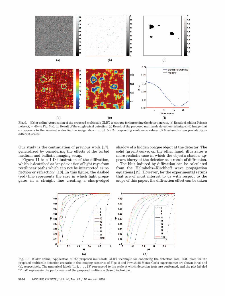
edge areas. Also, in Fig. 9(e) we see that the area withthe lowest confidence is the place where most mis-classifications happen. This is good news, since toincrease the detection rate, we may opt to do a second(and faster) round of scans, sampling only on thesevery low-confidence regions. In Figs. 8(f) and 9(f), weplot the misclassification rates at each scale (curve),and compare it with the overall multiscale rate (line).These numerically experimented plots show that theperformance of the proposed pixelwise GLRT tech-nique (depending on the noise level) is either veryclose to [Fig. 8(f)] or even better than [Fig. 9(f)] thebest fixed-scale technique. In Figs. 10(a) and 10(b),the performance of the single-pixel detection tech-nique is compared with the multiscale ones via theircorresponding ROC curves. Once again, the multi-scale technique shows the best or close to the bestperformance.

4. Diffraction Effects

So far in this paper, all detection tests and relatedperformance analysis were derived based on a sim-plified model of light propagation that ignores diffrac-tion. Although such approximation works well formany practical applications, it is not a suitable modelfor detecting or imaging relatively small sized objects.In this section, we present statistical analysis of theresolution limits in ballistic imaging systems by de-fining the smallest size of resolvable objects in a tur-bid medium at given false alarm and detection rates.

Fig. 7. (a) Ideal deterministic and noise-free image of four objectsof different sizes and shapes. (b) Corresponding image as a Pois-sonian noise-free stochastic signal, with Xs � 1.

Fig. 8. (Color online) Application of the proposed multiscale GLRT technique for improving the detection rate. (a) Result of adding Poissonnoise �Xe � 20� to Fig. 7(a). (b) Result of the single-pixel detection. (c) Result of the proposed multiscale detection technique. (d) Image thatcorresponds to the selected scales for the image shown in (c). (e) Corresponding confidence values. (f) Misclassification probability indifferent scales.


Our study is the continuation of previous work [17],generalized by considering the effects of the turbidmedium and ballistic imaging setup.

Figure 11 is a 1-D illustration of the diffraction,which is described as “any deviation of light rays fromrectilinear paths which can not be interpreted as re-flection or refraction” [18]. In this figure, the dashed(red) line represents the case in which light propa-gates in a straight line creating a sharp-edged

shadow of a hidden opaque object at the detector. Thesolid (green) curve, on the other hand, illustrates amore realistic case in which the object’s shadow ap-pears blurry at the detector as a result of diffraction.

The blur induced by diffraction can be calculatedfrom the Helmholtz–Kirchhoff wave propagationequations [19]. However, for the experimental setupsthat are of most interest to us with respect to thescope of this paper, the diffraction effect can be taken

Fig. 9. (Color online) Application of the proposed multiscale GLRT technique for improving the detection rate. (a) Result of adding Poissonnoise �Xe � 40� to Fig. 7(a). (b) Result of the single-pixel detection. (c) Result of the proposed multiscale detection technique. (d) Image thatcorresponds to the selected scales for the image shown in (c). (e) Corresponding confidence values. (f) Misclassification probability indifferent scales.

Fig. 10. (Color online) Application of the proposed multiscale GLRT technique for enhancing the detection rate. ROC plots for theproposed multiscale detection scenario in the imaging scenarios of Figs. 8 and 9 (with 25 Monte Carlo experiments) are shown in (a) and(b), respectively. The numerical labels “1, 4, . . . , 23” correspond to the scale at which detection tests are performed, and the plot labeled“Final” represents the performance of the proposed multiscale (fused) technique.


into account by convolving the expected signal valuewith an appropriate point-spread function (PSF) thatdescribes the blurring effect of an object estimatedfrom the Fraunhofer approximation. For a circularopaque object, such a PSF is given by

H�r� � 1 �2k�2

z sinkr2

2z

J1�k�rz �

k�rz

�k2�4

z2 J1�k�rz �

k�rz

�2

,

(15)

where k � 2�� is the wavenumber, J1� � is the order1 Bessel function of the first kind, � is the radius ofthe opaque object, r is the radius coordinate in thedetector plane, and z is the distance between theobject and the detector [20]. Note that the Fraunhoferapproximation is only valid when z �� 4�2��, andtherefore in this paper we only consider far-field im-aging scenarios. Ignoring the effect of a turbid me-dium and considering homogeneous illuminationwith intensity I� at the object plane, the radially sym-

metric intensity of the detected signal at the radiuscoordinate r is simply given by I � I�H�r�. Figure12(a) shows the diffraction pattern of a circularopaque object with a distance of z � 100 m from thedetector, illuminated by unit-intensity �I� � 1� lightwith 800 nm wavelength.

In the imaging scenarios considered in this paper,the detected signal is further attenuated by the tur-bid medium, and the expected value of the signalintensity at the radius coordinate r and distance zfrom the object plane can be approximated as

I � I� exp��tz�H�r�,

where we have ignored the fact that due to diffractionsome parts of the wavefront travel slightly longerdistances. Note that in practice, due to the far-fieldimaging assumption, such variance in attenuation issmall. This effect is shown in Fig. 12(b), where thepath lengths L1 and L2 are practically equal if thedistance between the opaque object and the detector(z) is significantly larger than the PSF spread. Thedetection problem associated with the signal modeldefined above is described in the following two imag-ing scenarios:

Y �0: An opaque object of unknown but small size�� 0� is hidden in the scattering medium, blockingand blurring the laser pulse (i.e., measurements con-tain noise plus attenuated and blurred laser pulse).

Y �1: No opaque object exists �� 0� in the prop-agation line of the laser pulse (i.e., measurementscontain noise plus attenuated laser pulse).

The above GLRT detector is different than the NPdetectors of Section 3 since the size of the object isnow assumed to be unknown. Following Eq. (2), theexpected value of the intensity in the absence of theobject ��1� is given by

I�k, 0� � I0e��td � Xe.

Fig. 11. (Color online) Shadow of an opaque object illuminated bya homogeneous widespread light beam. The dashed (red) curverepresents the intensity of the measured light ignoring diffraction.The solid (green) curve represents the diffraction-induced PSF.

Fig. 12. (Color online) (a) 1-D slice of the diffraction pattern of a circular object of radius 3 mm at 100 m distance and 800 nm wavelength.(b) 1-D slice of the imaging scenario, where z is the distance between the opaque circular object (radius �) and the detector. d is the distancebetween the laser and the detector. The pass length L1 � L2 when z is very long.


The intensity of the signal in the presence of theobject ��0� is estimated as

I�k, �̂� � I0e��tdH�rk� � Xe, (16)

where �̂ is the estimate of the opaque object’s radiusand rk is the radial distance of the kth pixel from theaxes passing through the center of the object. Theunknown radius of the opaque object is estimated as

�̂ � arg max�

�k�1

N e�I�k,��I�k, ��yk

yk! . (17)

The above ML estimate of the radius is solved bynumerical optimization, where we discretize � overan assumed range of values ��g, g � 1, . . . , G, andcompute the cost function,

|�g � k�1

N

yk log�I�k, ��g�� I�k, ��g�. (18)

The value of g for which |�g takes on the largestvalue is gmax, and finally the GLRT detection statis-tics is given by

k�1

N

yk log�I�k, ��gmax�I�k, 0� �� . (19)

As an illustrative example, by fixing the falsealarm rate at PFA � 0.1, the noise level at Xe � 20, andassuming a large detector that detects all the light,regardless of the distance or size of the object, weused the above GLRT framework to search for thesmallest detectable object size at different distancesand detection rates in heavy fog ��t � 12.5�1 m�1�.Figure 13 illustrates the result of this experiment,where as expected the size of detectable objects firstrises as the distance increases.

5. Laboratory Setup and Experiments

A. Conventional Ballistic Imaging Experimentation

In our experiments, to generate ultrashort opticalpulses we used a Coherent Mira 900 Ti:sapphire tun-able femtosecond laser pumped by an 8 W pump(Verdi V-8). At the output this laser generates anaverage power of �1 W with pulses of 200 fs duration,13 ns repetition period, and 830 nm wavelength.

As shown in Fig. 14, each laser pulse passesthrough a ��2 plate and is incident on a polarizingbeam splitter that divides the pulse into two copies,one used for triggering the ultrafast time gate whilethe other passes through the scattering medium(which is modeled by two sets of solid diffusers lo-cated in front and back of the target). Rotation of the��2 plate determines the power ratio between the twopulses, and we experimentally determined that thebest results are achieved in a near 50%�50% splittingratio. After passing through the diffusers and target,the ballistic photons are incident on the gate at ex-actly the same time as the triggering pulse and passthrough the ultrafast time gate, where due to thephase and polarization difference the scattered pho-tons are rejected. In practice, the triggering pulsetiming is controlled by a delay line, which increasesor decreases the optical path length, using acomputer-controlled translation stage.

The ultrafast time gate used is a nonlinear crystal,�-barium borate (BBO) [21], which utilizes a two-photon process such that the gating time can be asshort as the laser pulse width. Additionally, byslightly changing the incident angles of the twopulses on the nonlinear crystal, the time-gated resultcan be spatially separated from the background sig-nal, greatly increasing the signal-to-noise ratio. Thiseffect is sometimes referred to as background-freecross correlation [22]. The energy of the ballistic pho-tons are then measured by a silicon detector and alock-in amplifier. The entire setup implemented atthe ultrafast imaging laboratory at the University of

Fig. 13. (Color online) Detection rate versus the (unknown)opaque circular target’s radius and the distance between the laserand the detector considering the diffraction limit with PFA � 0.1and Xe � 20 in heavy fog ��t � 12.5�1 m�1�.

Fig. 14. (Color online) Laser setup at the Ballistic Imaging Lab-oratory at the University of California, Santa Cruz.


California, Santa Cruz, is controlled using LabViewand a general purpose interface bus (GPIB) bus.

Figure 15 shows the results of two imaging exper-iments where the objective is to read the text writtenon transparency sheets by a ballpoint pen, sur-rounded by a total of five solid glass (Thorlabs groundglass, DG10-220) diffusers. The thickness of thesediffusers is 2 mm each, with the MFP of 0.73 mm (7.3MFP total). We also note that the dynamic range ofour system is approximately 100 dB. Figures 15(a)and 15(b) show the result of scans in the absence andFigs. 15(c) and 15(d) show the result of scans in thepresence of the ballistic time gate, without any post-processing. To acquire the nongated images, the gatewas removed and the detector repositioned. Note thatFigs. 15(a) and 15(c) illustrate raw data (without anypostprocessing) from the imaging system, whereasthe results shown in Figs. 15(b) and 15(d) are eachupsampled by a factor of 3 via the bicubic interpola-tion technique. These results show that, althoughballistic images are noisier than the non-time-gated(diffusive) ones, they are preferable since they arevirtually blur free.

B. Adaptive Sampling Experimentation

As explained in the previous sections, in ballistic im-aging, 2-D images of the objects in the scatteringmedia are created by a relatively time-consumingpoint-by-point scanning scheme in which the field ofview (FOV) is sampled at regularly spaced locations.For instance, in a typical laboratory setup with amechanical translation stage (Fig. 14), creating a256 � 256 image (i.e., sampling at 65,536 points)

takes about 4 h, which might be prohibitively long formany real-world applications. Although such exces-sive time can be reduced if the mechanical transla-tion stage is replaced by a more expensive optical one,faster scans are always desired, and moreover, formany applications, the total number of pulses deliv-ered in a given time period is limited by the averagedelivered energy due to health concerns.

By making some simplifying assumptions aboutthe objects of interest (e.g., piecewise constancy), ir-regular scan strategies, such as sampling sparsely inthe low-frequency areas and densely in the high-frequency (edge or textured) areas, are shown to beuseful in reducing the imaging time. Recently, tworelated techniques, namely, compressive sensing[23,24] and active learning [25] (adaptive sampling)were proposed to reduce the number of samples re-quired to achieve certain reconstruction accuracywith respect to the regular (passive) scanning tech-nique. We note that it is the sparsity of the signal ofinterest (in a given overcomplete dictionary of bases)that enables such techniques to gather sufficient in-formation to achieve optimal (if not perfect) recon-struction in the presence of noise, even when thesampling rate is lower than the Nyquist rate [26]. Inthe compressive sensing technique, random projec-tions of the signal of interest onto an overcomplete setof basis functions are sequentially recorded. Suchrandom projections in practical optical imaging sce-narios can be implemented by passing a wide-fieldbeam through binary masks with a random pattern[in practice, a digital micromirror device can be usedto generate the random basis patterns [27]]. Unfor-tunately, in the ballistic imaging setup, creating awide-field beam is not easy. Moreover, diffraction lim-its the resolution of the binary mask and thereforeimplementing a compressive-sensing-based ballisticimaging system is not trivial. On the other hand, inthe following we show that adaptive sampling tech-niques can be readily exploited for ballistic imagingpurposes.

We have implemented adaptive sampling as a two-step process [28]. In the first step, we regularly sam-ple the FOV space at N�2 points, where N is the totalnumber of samples that we plan to collect. We usethese N�2 measurements to create a pilot estimate ofthe unknown FOV. In the next step, the remainder ofthe N�2 points are used to sample the FOV on theedge areas of the estimated image. It can be shownthat the decay rate of the mean square error for piece-wise constant images is O�N�1�2� and O�N�1� for thepassive and active sampling techniques, respectively[28].

We also note that active learning relies on accurateadaptive image reconstruction algorithms to recon-struct the unknown images from the irregular sam-ples of the FOV. In our implementation, we used animage reconstruction method based on maximuma posteriori (MAP) with bilateral total variation prior(regularizer) [29]. The general formulation of this

Fig. 15. (Color online) Comparison of diffusive and ballistic im-aging. (a), (b) Two diffusive (no time gating) scans. (c), (d) Twocorresponding ballistic (time-gated) scans through five solidground glass diffusers.


technique is presented as follows:

�̂X�t� � arg min�X�t�

��A��X��̂Z��22 � �

l,m��P

P

��m��l��X

�SxlSy

m�X�1�, (20)

where �X of size �ML � 1 is a vector representing thereconstructed image of size �M � L after lexico-graphic ordering, and �Z of size �ML � 1 is a vectorthat stores the N � ML measurements. In this vector,the elements that correspond to those pixels in X forwhich no measurement is available are filled withzeros. The matrices Sx

l and Sym are the operators

corresponding to shifting the image represented by �Xby l pixels in the horizontal direction and m pixels inthe vertical direction, respectively. The scalar weight,0 � � � 1, is applied to give a spatially decaying effectto the summation of the regularization terms, whichin effect represent derivatives across multiple reso-lution scales. Matrix A of size �ML � ML is a diag-onal matrix whose values are chosen in relation toour confidence in the measurements that contributedto make each element of �̂Z (diagonal elements corre-sponding to pixels for which no measurement is avail-able are replaced with zeros). The regularization

parameter, �, is a scalar for properly weighting thefirst term (data fidelity cost) against the second term(regularization cost).

To validate the applicability of this adaptive sam-pling and reconstruction technique versus the com-mon passive sampling technique, we performed thefollowing experiment. A metal washer was imagedthrough a ground glass diffuser (Thorlabs groundglass, DG10-220) via the ballistic imaging setup ofFig. 14. Figure 16(a) shows the result of scanning themedium on a 128 � 128 (16,384 total) regularly sam-pled grid. Figure 16(b) shows the same image sam-pled on a regular 32 � 32 (1024) grid and thenupsampled by the bicubic interpolation method to adense 256 � 256 grid. The alternative samplingstrategy was performed by exploiting the same ex-perimental setup (distance, turbid medium, target),where a total of 950 irregularly sampled data pointswere collected in the said two-step adaptive process.Figure 16(c) shows the result of such an adaptivesampling scheme after upsampling to the 256 �256 grid by the proposed adaptive MAP-based in-terpolation method. The spatial position of the 984adaptive samples are marked as white dots on a256 � 256 grid in Fig. 16(d), which, as expected, isconsiderably denser on the edge areas.

6. Conclusion and Future Work

In this paper, we have studied a technique for cap-turing high-resolution images through turbid media.This approach was based on separating the unscat-tered (ballistic) photons from the diffused ones byimplementing an ultrafast time-gating system. Thenovelty of this paper is in combining the recent ad-vances in optical science with the novel image pro-cessing and statistical signal processing techniques.We studied the resolution limits of such a system thatwere close to diffraction (Rayleigh) limits for longerdistances. We derived the fundamental limits on theaccuracy of the estimated extinction parameters of anunknown turbid medium and the targets inside it.This study also guided us toward the most efficientexperiments (with respect to both time and accuracy)for calibrating the model parameters of the unknownturbid medium as well as the optical properties of thetarget (which can be used to identify and categorizeit). Our results showed that for a medium of practicalinterest, namely, heavy fog, optical parameters canbe estimated with high accuracy. We used the saidmodel to derive optimal statistical tests for detectingobjects hidden in turbid media. Performance analysiswas carried out by computing ROC curves for theproposed optimal tests, showing that, by consideringonly the ballistic photons, we are able to detectopaque objects hidden in heavy fog in the range ofapproximately 380 m (i.e., 30 MFPs). The detectionrate of the semitransparent objects is shown to beslightly less than this distance. Also, real experi-ments attested to the fact that ballistic imaging, es-pecially in longer distances, is difficult, and thereforewe developed a multiscale GLRT algorithm to im-prove the detection rate in such scenarios. To reduce

Fig. 16. Comparison of passive and active imaging. (a) Result ofscanning the turbid medium on a regular 128 � 128 grid (16,384dense passive sampling). (b) Result of scanning the turbid mediumon a regular 32 � 32 grid (1024 sparse passive sampling) followedby interpolation via bicubic interpolation to reconstruct the imageon a 256 � 256 grid. (c) Result of scanning the turbid medium onan irregular grid (984 sparse adaptive sampling) followed by in-terpolation via adaptive interpolation to reconstruct the image ona 256 � 256 grid. (d) Distribution of the 984 irregular samples.


the data acquisition time that is essential for manyreal-world applications, we implemented an adaptivesampling scheme that significantly reduced the dataacquisition time.

As for future work, one may exploit temporal, spa-tial, and wavelength diversity and coding for ballisticimaging. We can study the array imaging frameworkwhere multiple emitters will transmit coordinatedpulses of light, and for their part, a collection ofphoton-detecting elements will gather the receiveddata and compute a resultant image. Furthermore,there is the possibility of analyzing various ways ofcoding these pulses (e.g., transmitting sequences ofpulses as is done in ultrawideband communications).

Moreover, we believe that detection techniquesthat exploit all ballistic, snake, and diffused photons[30] (what we term holistic imaging and detection)enable detection of larger objects at significantlylonger range. More theoretical and experimentalwork needs to be done to design a (near) optimal yetpractical solution to this important problem.

Appendix A: Decision-Theoretic Resolution Bounds

As explained throughout this paper, the diffraction-limited resolution of ballistic imaging systems [e.g.,Figs. 15(c) and (d)] makes them appealing for imag-ing in relatively short distances. However, in rela-tively long distances the ballistic signal is too weakand we are bound to rely on the blurry but highersignal-to-noise ratio (SNR) images of conventionalimaging systems [e.g., Figs. 15(a) and (b)]. In thisAppendix, we adapt a decision-theoretic approach tothe resolution bounds and search for the critical dis-tance after which the ballistic imaging systems are ofno practical advantage compared with the conven-tional imaging systems.

1. Ballistic Imaging—Single Point

The problem of determining whether an object liesalong the line of sight can be cast as a statisticalhypothesis test as follows. Given a received photoncount X at the sensor, one must choose between twopossible situations. The first situation is that no oc-cluding object exists in the path between the laserand the sensor ��0�. The alternative is that there is anoccluding object along the line of sight between thelaser and the detector ��1�. Semitransparent objectscan be considered to be significantly more scatteringthan the medium [31], and therefore the detector willcollect an attenuated number of ballistic photons(compared with �0) along with the noise photons.

Following the notation of Subsection 3.B, we definethe number of noise photons that will arrive at thedetector as ��NXe�, where X � �� is a Poisson-distributed random variable with mean �. Then, thehypothesis test is given by the null hypothesis de-fined as �0 : X � ��NXe � NXs� and the alternatehypothesis (object exists) defined as �1 : X � ��NXe

� NXsinc�. As the mean of the Poisson distribution

grows, the probability distribution tends to a Gauss-ian, e.g., averaging many repeated Poissonian trials(i.e., N large) results in a Gaussian-distributed sta-

tistic. Using the Anscombe transformation [31], weobtain the following relationship:

X � �� ) 2�X �38 � ��2��, 1�,

where ��, �2� represents Gaussian distribution withmean � and variance �2. Defining a new variablerepresenting the Anscombe-transformed statistic X�� 2�X � 3�8 the hypothesis test becomes

�0 : X� � ��2�NXe � NXs, 1�,

�1 : X� � ��2�NXe � NXsinc, 1�. (A1)

The decision test is now defined as �X� � �0

�1 ��,where a user-specified false alarm rate �PFA� deter-mines the value of the threshold � �� such that P�X�� 0� � PFA.

2. Ballistic Imaging—K Points

The problem now is modified to describe an imagingscenario of scanning the FOV at a fixed square arrayof ��K � �K� points. This results in a multiple hypoth-esis testing problem (K tests), where for large K itputs a lower bound on the SNR of the observation. Toboost the SNR, one could use spatial aggregation byaveraging over a number of observation points. Thismodifies the problem to averaging neighborhoods ofpoints in an area measuring �W � �W, W � K, effec-tively reducing the spatial resolution of the detectionmap (image). By decreasing the spatial resolution,this also decreases the variance at each point, modi-fying the decision test to

�0 : X� � ��2�NXe � NXs,1W�,

�1 : X� � ��2�NXe � NXsinc,

1W�. (A2)

This test is under the assumption that the averag-ing window will contain either no occluder points orall occluder points. In reality, the averaging filter willresult in an observed point, X� � ��E�X�|�0 ��1 � ��E�X�|�1, 1�W�, where � is the fraction of thewindow containing nonoccluders, and E is the ex-pected value operator. Our goal is to find the lowerbound on the value of W that will guarantee an over-all false alarm rate of less than PFA, and we onlyconsider the ideal case (all occluders or nonoccluders)in our calculations in order to obtain closed-form so-lutions.

The Bonferroni correction approach is a con-servative method of controlling the false alarm ratefor a detection problem under multiple independentand identically distributed tests [33]. The correc-tion adjusts the threshold for each individual test inorder to satisfy a lower (per test) false alarm rate


value �PFA�K� such that each of the fixed number Kpoints in the array (and W-point averaging filter)satisfies �P�X � �|�0� � PFA�K. With ��x� as thecumulative distribution function of the ��0, 1�density at the point x, this results in � � ��1��W��1�PFA�K� � 2�NXe � NXs. To give a satis-factory observation, we also bound the miss probabil-ity for detecting a ballistic photon by the samemodified value �PFA�K� such that �P�X �|�1�� PFA�K. Using the miss bounds, we determine thelower bound on the necessary averaging window size(W) to image a fixed K-point array as

W � 12 ��1�1 �PFA

K �� 1�PFA

K ��NXe � NXs � �NXe � NXsinc

�2

. (A3)

The minimum width of the occluding object �wb�that can be reliably resolved for a given parameter-ized turbid medium can now be derived. Using thelower bound for W found in Eq. (A3), we can solvefor the lower bound on the width using wb ��FOV � W��K.

3. Conventional Imaging Analysis

In the conventional imaging regime, there is no time-gating mechanism and all the photons that reach thedetector over a long acquisition time will be observed[acquisition time �� (d�c) direct line-of-sight flighttime]. Therefore, a large number of photons sentthrough the medium will be collected by the detector.A problem occurs here, too—although the SNR is highdue to the large number of photons, the average num-ber of scattering events on each photon collected will

Fig. 17. Simulation experiments with FOV � 50 m � 50 m, dinc � 0.3 m, and �t � 12.5�1 m�1. (a)–(c) Ballistic, Bonferroni, andconventional observations at d � 350 m, respectively. (d)–(f) Ballistic, Bonferroni, and conventional observations at d � 400 m, respec-tively. (g)–(i) Ballistic, Bonferroni, and conventional observations at the critical distane d � dcritical � 417 m, respectively.


also be high. As the number of scattering events in-creases for a photon, the spatial resolution of theoccluding object will degrade. The lack of spatial in-formation results in a blurred observation. Usingrandom-walk theory [34,35], it is possible to solve forthe minimum width of an occluding object that is re-liably resolved using a conventional imaging system.The width [36] is found using the photon mean time offlight ��t�, which can be numerically computed as afunction of the parameters of the medium ��s, �a�.The modified minimum full width at half-maximum(FWHM) is equal to wconv � 0.94��t�c��s�1�2.

4. Optimal Resolution Trade-Offs

Ideally, one should choose the imaging system (bal-listic or conventional) that reliably resolves thesmallest possible object �w � min�wconv, wb�. The de-cision test using the minimum resolvable sizes de-rived above becomes

wconv �ballistic

conventionalwb ) 0.94��t�c

�s�1�2

�ballistic

conventional�FOV � WK .

(A4)

Using the lower bound of W from Eq. (A3), one cansolve for the critical distance �d � dcritical�, the maxi-mum distance at which ballistic still offers superiorresolution relative to conventional imaging.

As an illustrative example, we considered a ballis-tic scanning experiment at �K � 2562� points, imaginga 50 m � 50 m FOV. The occluding objects were as-sumed to be circular of diameter 1.0, 2.0, 4.0, 10.0,and 20.0 m each of thickness dinc � 0.3 m and �inc

� 12.5 m�1. We used false alarm rate PFA � 0.05 andconsidered a heavy fog turbid medium with �t �12.5�1 m�1. Using the analysis from above, dcritical �417 m, which is consistent with earlier results weshowed in Section 3. Figure 17 shows the effect ofdistance on the ballistic resolution, illustrating thecaptured ballistic and diffused (conventional) imagesat distances of d � 350, 400, 417 m.

The authors wish to thank Ines Delfino, HeikeLischke, and Mohammad Alrubaiee for providinginvaluable information and data throughout thisproject. This work was supported in part by DefenseAdvanced Research Projects Agency, Air Force Of-fice of Scientific Research grant FA9550-06-1-0047.Approved for public release; distribution unlimited.

References1. C. Dunsby and P. M. W. French, “Techniques for depth-

resolved imaging through turbid media including coherence-gated imaging,” J. Phys. D 36, 207–227 (2003).

2. K. Yoo and R. R. Alfano, “Time-resolved coherent and incoher-ent components of forward light scattering in random media,”Opt. Lett. 15, 320–322 (1990).

3. A. F. Fercher, W. Drexler, C. K. Hitzenberger, and T. Lasser,“Optical coherence tomography —principles and applications,”Rep. Prog. Phys. 66, 239–303 (2003).

4. M. E. Zevallos, S. K. Gayen, M. Alrubaiee, and R. R. Alfano,

“Time-gated backscattered ballistic light imaging of objectsin turbid water,” Appl. Phys. Lett. 86, 0111151–0111153(2005).

5. M. Paciaroni and M. Linne, “Single-shot, two-dimensional bal-listic imaging through scattering media,” Appl. Opt. 43, 5100–5109 (2004).

6. D. Contini, F. Martelli, and G. Zaccanti, “Photon migrationthrough a turbid slab described by a model based on diffusionapproximation. I. Theory,” Appl. Opt. 36, 4587–4599 (1997).

7. I. Delfino, M. Lepore, and P. L. Indovina, “Experimental testsof different solutions to the diffusion equation for optical char-acterization of scattering media by time-resolved transmit-tance,” Appl. Opt. 38, 4228–4236 (1999).

8. W. Cai, S. K. Gayen, M. Xu, M. Zevallos, M. Alrubaiee, M. Lax,and R. R. Alfano, “Optical tomographic image reconstructionfrom ultrafast time-sliced transmission measurements,” Appl.Opt. 38, 4237–4246 (1999).

9. B. B. Das, F. Liu, and R. R. Alfano, “Time-resolved fluorescenceand photon migration studies in biomedical and model randommedia,” Rep. Prog. Phys. 60, 227–292 (1997).

10. A. Gibson, J. Hebden, and S. Arridge, “Recent advances indiffuse optical imaging,” Phys. Med. Biol. 50, R1–R43 (2005).

11. H. Lischke, T. J. Loeffler, and A. Fischlin, “Aggregation ofindividual trees and patches in forest succession models: cap-turing variability with height structured, random, spatial dis-tributions,” Theor. Popul. Biol. 54, 213–236 (1998).

12. S. V. Aert, D. V. Dyck, and A. J. den Dekker, “Resolution ofcoherent and incoherent imaging systems reconsidered—classical criteria and a statistical alternative,” Opt. Express14, 3830–3839 (2006).

13. S. M. Kay, Fundamentals of Statistical Signal Processing: Es-timation Theory (Prentice-Hall, 1993), Vol. 1.

14. L. L. Scharf, Statistical Signal Processing: Detection, Estima-tion, and Time Series Analysis (Addison-Wesley, 1991).

15. G. W. Sutton, “Fog hole boring with pulsed high-energylasers—an exact solution including scattering and absorption,”Appl. Opt. 17, 3424–3430 (1978).

16. S. M. Kay, Fundamentals of Statistical Signal Processing De-tection Theory (Prentice-Hall, 1998), Vol. 2.

17. M. Shahram and P. Milanfar, “Imaging below the diffractionlimit: a statistical analysis,” IEEE Trans. Image Processing13, 677–689 (2004).

18. A. Sommerfeld, Optics Lectures on Theortical Physics (Aca-demic, 1954), Vol. 4.

19. J. Goodman, Introduction to Fourier Optics, 3rd ed. (Robertsand Company, 2005).

20. G. B. Parrent, Jr. and B. J. Thompson, “On the Fraunhofer (farfield) diffraction patterns of opaque and transparent objectswith coherent background,” J. Mod. Opt. 11, 183–193 (1964).

21. D. N. Nikogosyan, “Beta barium borate (BBO),” Appl. Phys. A52, 359–368 (1991).

22. M. Ghotbi and M. Ebrahim-Zadeh, “Optical second harmonicgeneration properties of BiB3O6,” Opt. Express 12, 6002–6019(2004).

23. E. Candès, J. Romberg, and T. Tao, “Stable signal recoveryfrom incomplete and inaccurate measurements,” Commun.Pure Appl. Math. 59, 1207–1223 (2006).

24. J. Haupt and R. Nowak, “Signal reconstruction from noisyrandom projections,” IEEE Trans. Inf. Theory 52, 4036–4048(2006).

25. R. Castro, J. Haupt, and R. Nowak, “Compressed sensing vs.active learning,” in 2006 International Conference on Acous-tics, Speech and Signal Processing (IEEE, 2006), pp. 820–823.

26. D. Donoho, M. Elad, and V. Temlyakov, “Stable recovery ofsparse overcomplete representations in the presence of noise,”IEEE Trans. Inf. Theory 52, 6–18 (2006).

27. M. Wakin, J. Laska, M. Duarte, D. Baron, S. Sarvotham, D.


Takhar, K. Kelly, and R. Baraniuk, “An architecture for com-pressive imaging,” in 2006 International Conference on ImageProcessing (IEEE, 2006), pp. 1273–1276.

28. R. Castro, R. Willett, and R. Nowak, “Faster rates in regres-sion via active learning,” in 2005 Advances in Neural Informa-tion Processing Systems 18 (MIT Press, 2005), pp. 179–186.

29. S. Farsiu, D. Robinson, M. Elad, and P. Milanfar, “Fast androbust multi-frame super-resolution,” IEEE Trans. Image Pro-cessing 13, 1327–1344 (2004).

30. B. Eriksson and R. Nowak, “Maximum likelihood methods fortime-resolved imaging through turbid media,” in 2006 Inter-national Conference on Image Processing (IEEE, 2006), pp.641–644.

31. S. Fantini, S. Walker, M. Franceschini, M. Kaschke, P. Schlag,and K. Moesta, “Assessment of the size, position, and optical

properties of breast tumors in vivo by noninvasive opticalmethods,” Appl. Opt. 37, 1982–1989 (1998).

32. F. Anscombe, “The transformation of Poisson, binomial andnegative-binomial data,” Biometrika 35, 246–254 (1948).

33. R. Miller, Simultaneous Statistical Inference (Springer, 1991).34. A. Gandjbakhche, G. Weiss, R. Bonner, and R. Nossal, “Photon

path-length distributions for transmission through opticallyturbid slabs,” Phys. Rev. E 48, 810–818 (1993).

35. A. Gandjbakhche, R. Nossal, and R. Bonner, “Resolution limitsfor optical transillumination of abnormalities deeply embed-ded in tissues,” Med. Phys. 21, 185–191 (1994).

36. V. Chernomordik, R. Nossal, and A. Gandjbakhche, “Pointspread functions of photons in time-resolved transilluminationexperiments using simple scaling arguments,” Med. Phys. 23,1857–1861 (1996).


statistical detection and imaging of objects hidden in...

Documents