statistical analysis of alcohol-related driving trends - nhtsa
TRANSCRIPT
DOT HS 810 942 May 2008
Statistical Analysis ofAlcohol-Related DrivingTrends 1982-2005
This document is available to the public from the National Technical Information Service Springfield Virginia 22161
The United States Government does not endorse products or manufacturers Trade or manufacturersrsquo names appear only because they are considered essential to the object of this report
ii
Technical Report Documentation Page 1 Report No
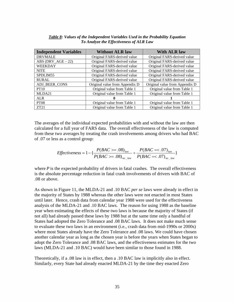
DOT HS 810 942
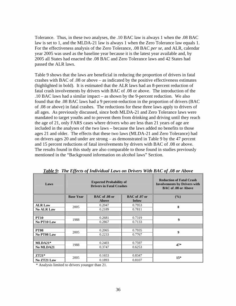
2 Government Accession No 3 Recipientrsquos Catalog No
4 Title and Subtitle
STATISTICAL ANALYSIS OF ALCOHOL-RELATED DRIVING TRENDS 1982-2005
5 Report Date
May 2008 6 Performing Organization Code
7 Author(s)
Jennifer N Dang
8 Performing Organization Report No
9 Performing Organization Name and Address
Evaluation Division National Center for Statistics and Analysis National Highway Traffic Safety Administration Washington DC 20590
10 Work Unit No (TRAIS)
11 Contract or Grant No
12 Sponsoring Agency Name and Address
Department of Transportation National Highway Traffic Safety Administration 1200 New Jersey Avenue SE Washington DC 20590
13 Type of Report and Period Covered
NHTSA Technical Report 14 Sponsoring Agency Code
15 Supplementary Notes
Overall the percent of drivers involved in fatal crashes who had consumed alcohol and had blood alcohol concentration (BAC) of 08 or above prior to the crash steadily decreased from 1982 to 1997 and then leveled off (more or less) In an attempt to explain the 1982-1997 reduction and the 1997-2005 level trend this report presents a statistical analysis of factors that influenced the historical alcohol-related driving trends from 1982 to 2005
The study is based on disaggregate logistic regression of imputed Fatality Analysis Reporting System (FARS) cases from all 50 States and the District of Columbia ndash to predict the probability of an alcohol-related involvement given a set of independent variables The independent variables include alcohol-related legislation (ie 10 BAC 08 BAC Administrative License Revocation minimum-legal-drinking-age laws) demographic factors (ie driverrsquos age and gender) per capita alcohol consumption and external factors (ie day of the week time of day roadway function class and posted speed limit)
The independent variables explain both the decrease in alcohol-related fatal crashes (where drivers involved in fatal crashes had BAC of 08 or above) from 1982 to 1997 and its leveling off after 1997 Large portions of the reduction are explained by the effect of alcohol-laws and by the demographic trends ndash the aging of the population and the increased proportion of female drivers The leveling off after 1997 does not imply that the laws are becoming less effective On the contrary they effectively maintain the proportion of drivers in fatal crashes who had BAC of 08 or above at the time of the crash ndash at the lowest level since 1982
17 Key Words
NHTSA FARS alcohol-related driving trends alcohol-related fatal crashes statistical analysis evaluation impaired driving fatality reduction
18 Distribution Statement
Document is available to the public at the Docket Management System of the US Department of Transportation httpdmsdotgov
19 Security Classif (Of this report)
Unclassified
20 Security Classif (Of this page)
Unclassified
21 No of Pages
69
22 Price
Form DOT F 17007 (8-72) Reproduction of completed page authorized
TABLE OF CONTENTS
TABLE OF CONTENTS iii
LIST OF ABBREVIATIONS iv
EXECUTIVE SUMMARY v
MOTIVATION FOR THIS STUDY1
METHOD 12 bull MULTIPLE IMPUTATION METHOD bull DEPENDENT VARIABLE bull INDEPENDENT VARIABLES
frac34 DEMOGRAPHIC AND EXTERNAL VARIABLES frac34 ADJUSTED PER CAPITA ALCOHOL CONSUMPTION frac34 PROGRAMMATIC INDEPENDENT VARIABLES
ALCOHOL-RELATED LEGISLATION frac34 OTHER POTENTIAL INDEPENDENT VARIABLES
bull ANALYZING THE MULTIPLE-IMPUTED DATASETS IN FARS bull LOGISTIC REGRESSION
RESULTS 25
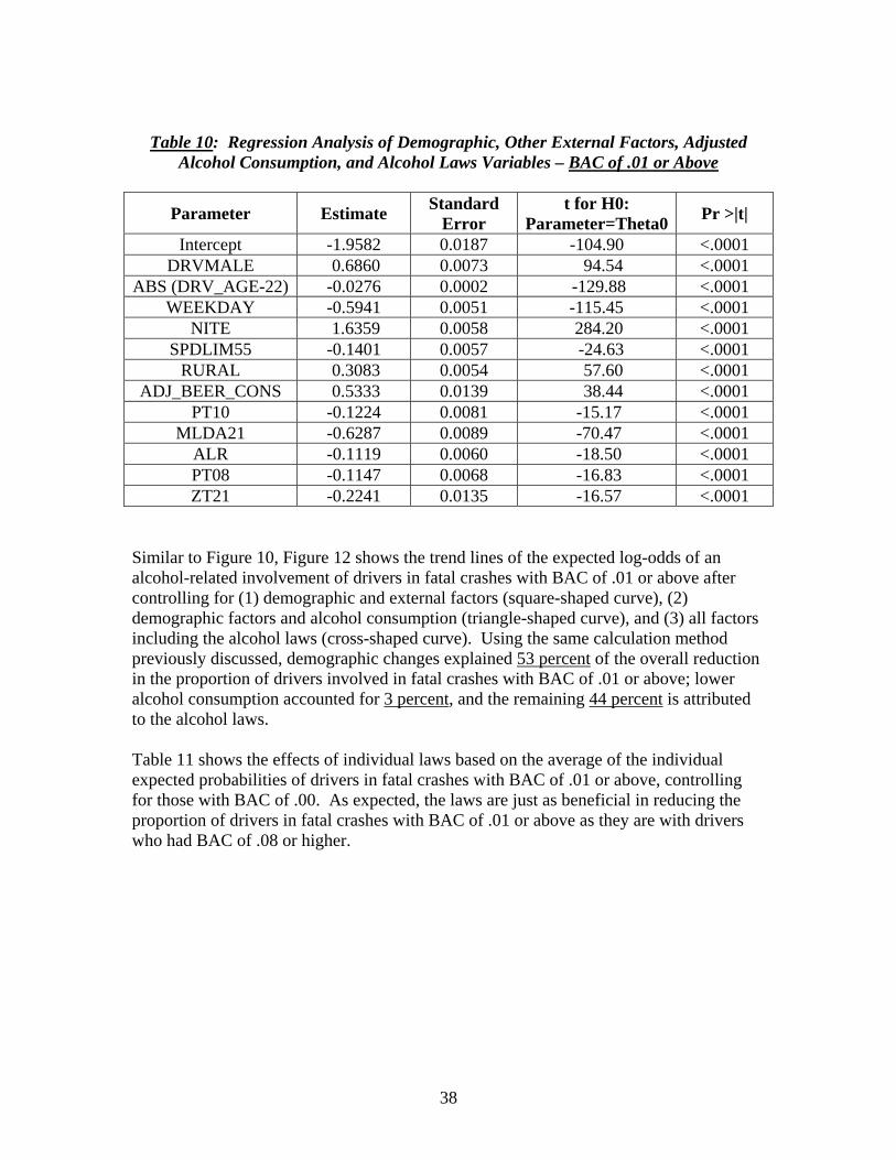
ANALYSIS OF ALCOHOL-RELATED DRIVING TRENDS INVOLVING 37 DRIVERS WITH BAC OF 01 OR ABOVE
CONCLUSIONS40
REFERENCES 42
APPENDIX A45
APPENDIX B 47
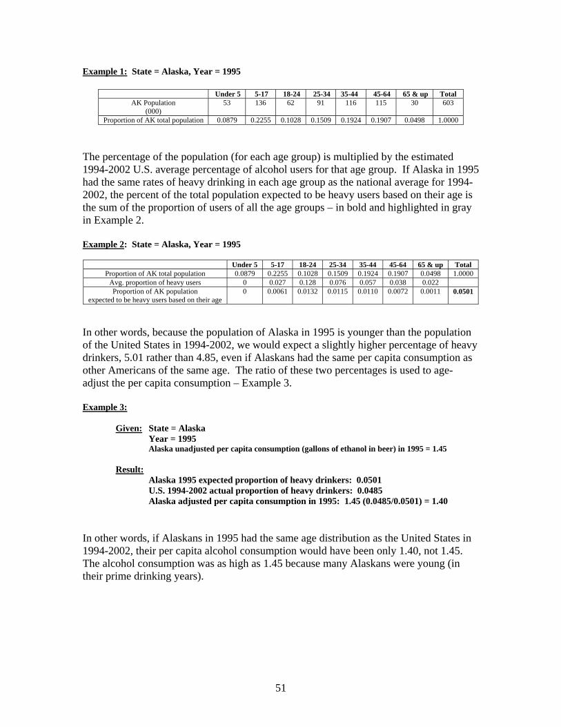
APPENDIX C 50
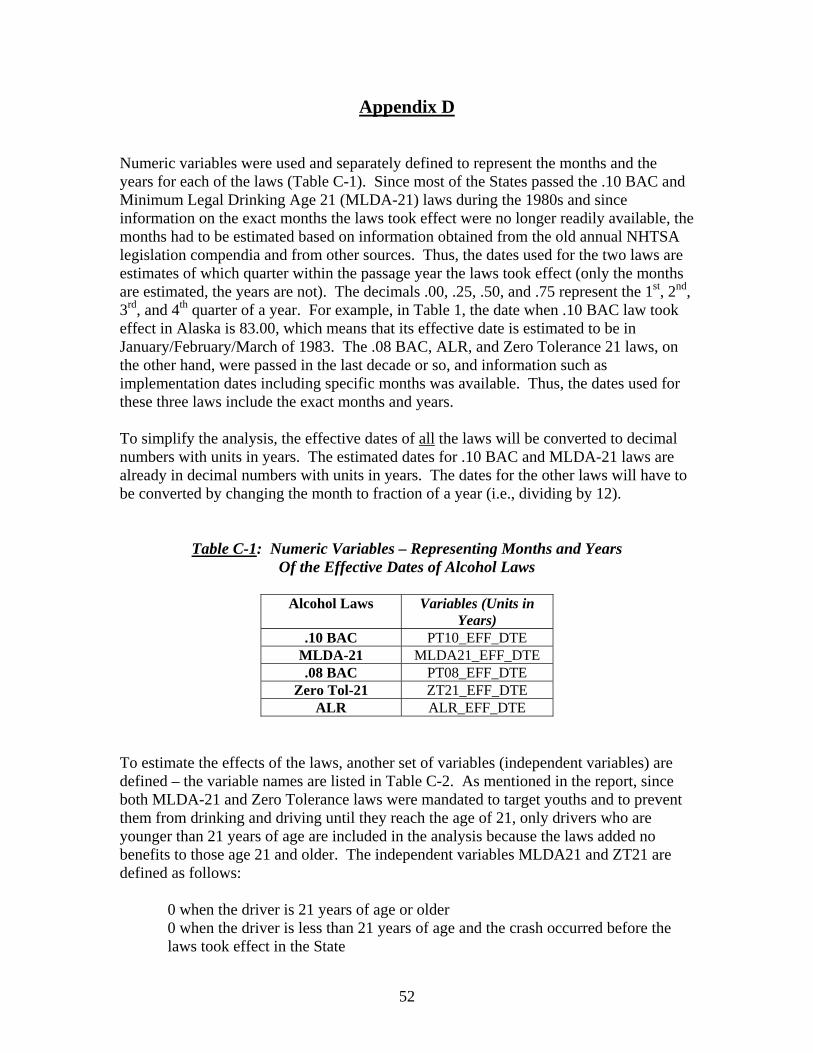
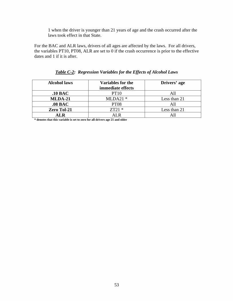
APPENDIX D52
APPENDIX E 54
iii
LIST OF ABBREVIATIONS
ALR Administrative License Revocation
BAC Blood alcohol concentration
DUI Driving under the influence
FARS Fatality Analysis Reporting System
MADD Mothers Against Drunk Driving
MLDA-21 Minimum Legal Drinking Age 21
NHTSA National Highway Traffic Safety Administration
SADD Students Against Destructive Decisions
SAS Statistical analysis software produced by SAS Institute Inc
iv
Figure 1 Actual Proportion of Drivers in Fatal Crashes with BAC = 08 or Above 1982-2005
0180
0200
0220
0240
0260
0280
0300
0320
0340
0360
0380
1982
1983
1984
1985
1986
1987
1988
1989
1990
1991
1992
1993
1994
1995
1996
1997
1998
1999
2000
2001
2002
2003
2004
2005
CY
Prop
ortio
n of
Dri
vers
in F
atal
Cra
shes
Cra
shes
0200
0350 Actual Proportion of Drivers (BAC of 08 or above)
EXECUTIVE SUMMARY
The number of fatal crashes that involved drivers who had been drinking at the time of the crash has decreased during the past two decades The proportion of crash fatalities that are alcohol-related ndash that occurred in crashes where at least one of the drivers andor nonoccupants involved had a blood alcohol concentration (BAC) of 08 or above ndash decreased at a steady rate from 53 percent in 1982 to 34 percent in 1997 It leveled off for two years and then increased by 1 percent in 2000 and remained at that level for two more years before it decreased to 33 percent in 2005 The proportion of drivers involved in fatal crashes who had BAC of 08 or above decreased from 35 percent in 1982 to 20 percent in 1997 and leveled off thereafter as shown in Figure 1
Tireless efforts were made in the last 20 years through legislative enactments and programs that were funded by States communities and private organizations to deter impaired driving These alcohol programs and laws served as a general deterrent to all those who drink and drive by sending a message that the States were getting tougher on impaired driving and hence these efforts made people think twice about getting behind the wheel after they had been drinking In fact the directional trend of the proportion of alcohol-related crash fatalities involving a driver andor nonoccupant with BAC of 01 or above is similar to the crash fatality trend where the BAC of a crash-involved driver
v
andor nonoccupant is 08 or above Moreover the directional trend of the proportion of drivers in fatal crashes with BAC of 01 or higher is similar to the trend in Figure 1
In 1998 the National Highway Traffic Safety Administration (NHTSA) contracted with a group of researchers (Voas and Tippetts) to study the ldquoRelationship of Alcohol Safety Laws to Drinking Drivers in Fatal Crashesrdquo Information on drivers in fatal crashes with positive BAC values for all 50 States and the District of Columbia from 1982 to 1997 was extracted from the Fatality Analysis Reporting System (FARS) and missing BAC data were imputed using Kleinrsquos methoddiams That analysis attributed a substantial benefit to laws that deter impaired driving However the study period was limited to the years where alcohol-related fatal crashes were steadily decreasing (1982-1997) and before they leveled off Post-1997 FARS data are now available The leveling off of the alcohol-related driving trend raised questions as to whether these alcohol programs are still as effective in deterring impaired driving as they were before NHTSA has embarked on this update and modification of Voas and Tippettsrsquos analysis
This study uses logistic regression analysis to (1) provide clarification to the change in the historical alcohol-related driving trends ndash why they steadily decreased from 1982 to 1997 and why they leveled off after that period and (2) assess the effects of alcohol programs that directly and indirectly changed public attitudes and behavior toward drinking and driving during the last 20 years In the first analysis this study calibrates the probability that a driver involved in a fatal crash had a BAC of 08 or above Since the two trends (specifically the proportion of drivers in fatal crashes with BAC of 08 or above and those with BAC of 01 or higher) are very similar this study also predicts (in the second analysis) the likelihood that a driver involved in a fatal crash had a BAC of 01 or above Logistic regression explores each driver as an individual in order to calibrate the effects of legislation to deter alcohol-related driving while controlling for demographic factors (ie driverrsquos age gender) external factors (ie whether or not the crash occurred at night on a weekday on a rural roadway and on a roadway with posted speed limit of 55 or greater) and per capita alcohol consumption By contrast the study by Voas and Tippetts aggregated the data by State and year making it more difficult to isolate the effect of demographic and external factors that vary from crash to crash This study is based on 1982-2005 FARS data for the 50 States and the District of Columbia
that include the estimates of alcohol involvement generated using Multiple Imputation
diams Kleinrsquos method was the method being used in FARS at the time of Voasrsquo and Tippettsrsquo study to estimate BAC distributions for drivers with unknown BAC test results It would calculate the probability that drivers in fatal crashes ndash where police reported alcohol information is unknown ndash had a BAC in grams per deciliter (gdL) of 00 01-09 or 10+ For additional information please refer to Klein T A Method for Estimating Posterior BAC Distributions for Persons Involved in Fatal Traffic Accidents NHTSA Technical Report No DOT HS 807 094 Washington 1986 These 51 jurisdictions are all called ldquoStatesrdquo in the discussion that follows
vi
when the BAC of drivers involved in fatal crashes is not explicitly reported a technique that has superseded Kleinrsquos imputation method
For both groups of drivers involved in fatal crashes (ie BAC of 08 or above and BAC of 01 or above) this study found that the 1982-1997 reductions in alcohol-related driving and the nearly level trends in 1997-2005 can be explained by the following
bull The benefits of five major types of State legislation to deter alcohol-related driving All or most of these laws were in effect in the majority of States by 1997
1) 10 BAC laws make it illegal to operate a motor vehicle at or above 10 gdL Most of the States passed this law during the 1980s All 50 had passed 10 laws by 1997
2) 08 BAC laws make it illegal to operate a motor vehicle at or above 08 gdL By 1997 16 out of 51 States had enacted this law and by 2005 every State had
3) Administrative License Revocation (ALR) laws revoke or suspend the driverrsquos license of an individual who refuses to submit to a BAC test or fails a test By 1997 40 out of 51 States had passed this law
4) Minimum Legal Drinking Age 21 (MLDA-21) laws make it illegal for an individual under the age of 21 to drink This law went into effect in every State during the 1980s
5) Zero Tolerance laws make it illegal for an individual under the age of 21 to operate a vehicle with a BAC level of 02 or more By 1997 47 out of 51 States had passed this lawlowast
bull The decreasing proportion of population age 18-34 from 1982 to 1999 leveling off thereafter
bull The increasing proportion of licensed female drivers from 1982 to 1997 leveling off thereafter Female drivers are generally much less likely to drink and drive than males
bull A small reduction in per capita alcohol consumption
Logistic regression models make it possible to tease out the relative contributions of legislation demographics and per-capital alcohol consumption to the reduction in the proportion of drivers in fatal crashes who had BAC of 08 or above (first analysis) and
Multiple imputation method is the method currently used in FARS to handle missing BAC data It imputes ten specific values of BAC across the full range of possible values for each missing value rather than estimating probabilities lowast Currently all 50 States and the District of Columbia have passed Zero Tolerance laws
vii
those who BAC of 01 or above (second analysis) and to track the contributions over time Figure 2 shows trend lines of predicted probability of an alcohol-related involvement of drivers in fatal crashes with BAC of 08 or above by models using none some or all of the factors considered in the logistic regressions
The horizontal line near the top of Figure 2 depicts the [unchanged] expected proportion of alcohol-related fatal crash involvements from 1982 to 2005 if (1) no new alcohol laws had gone into effect after December 31 1981 (2) the public attitudes about alcohol had not changed and (3) the driving population had not aged or otherwise changed Hence the expected proportion of drivers in fatal crashes with BAC of 08 or higher remains at 0349 from 1982 through 2005
The lowest curve in Figure 2 (short dashes of uniform length) shows the trend line predicted by the model controlling for all factors including the laws The expected proportion of drivers with a BAC of 08 or above decreases from 0336 in 1982 to 0214 in 1998 and somewhat levels off afterward (actually it slightly decreases to 0207 in 2005) This predicted trend closely follows the actual statistics shown in Figure 1
The uppermost curve in Figure 2 (alternating long and short dashes) is the trend predicted by a model that includes the demographic factors but not the variables on State laws and per capita alcohol consumption In other words it predicts what might have happened if the driving population had decreasing proportions of young andor male drivers ndash as happened in reality ndash but State laws and per capita alcohol consumption had remained exactly the same as they were on December 31 1981 This curve decreases from 0349 in 1982 to 0274 in 1998 and slightly increases to 0278 in 2005 The curve shows how favorable demographic trends in 1982-1997 would by themselves have accounted for a substantial proportion of the overall reduction ndash even in the absence of programs to reduce alcohol-related driving But because those demographic trends somewhat leveled off circa 1998 and one may even argue that there is a slight reversal in the trend toward an aging driver population so did the non-uniform dashed curve The light dotted region (upper portion of the graph) between the horizontal line and the non-uniform dashed curve denotes the year-by-year contribution of demographic factors to the overall reduction in the proportion of drivers in fatal crashes with BAC of 08 or greater
The middle curve in Figure 2 (long dashes) is the trend predicted by a model that includes demographic factors and per capita alcohol consumption but not State laws It predicts what might have happened if demography and per capita alcohol consumption had changed as really happened ndash but State laws had remained exactly the same as they were on December 31 1981 This curve decreases from 0349 in 1982 to 0269 in 1998 and levels off thereafter Per capita consumption decreased from 1982 to1997 but the true reduction was relatively small after taking into account that the population was aging at the same time The dark region (middle portion of the graph) between this curve and the one above it denotes the small contribution of reduced alcohol consumption to the overall decline in the proportion of drivers with BAC of 08 or above in fatal crashes
viii
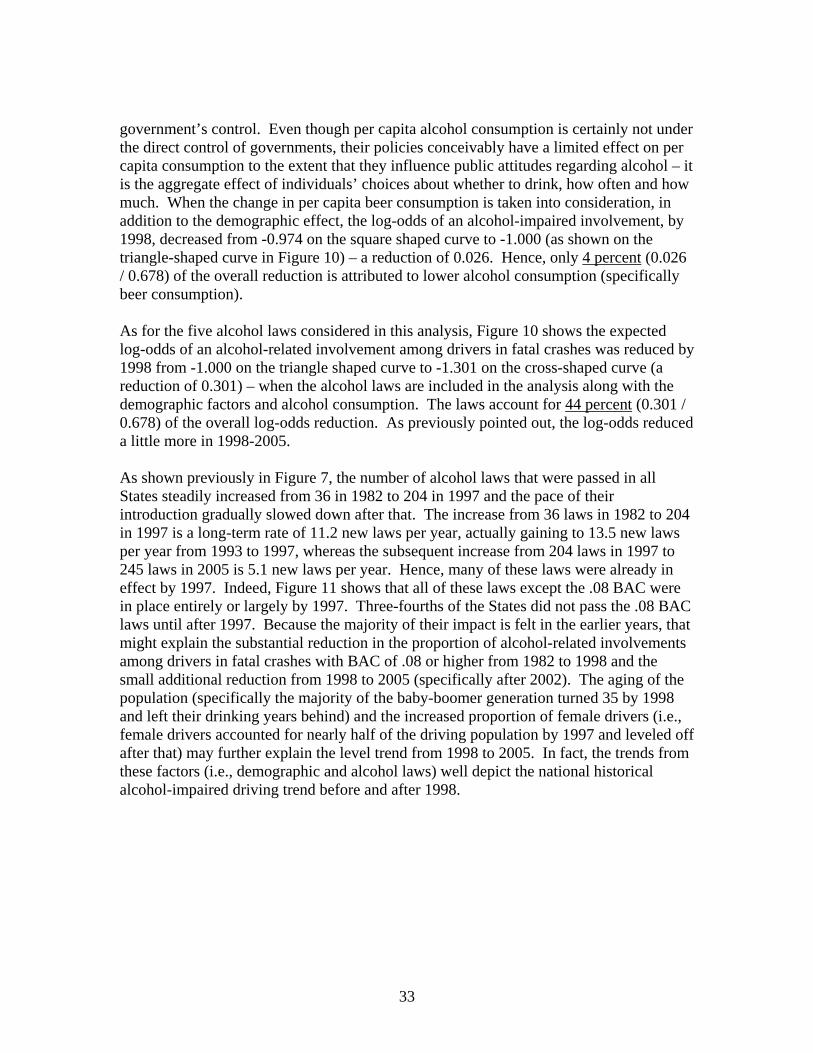
Finally the light diamond shaped region (bottom portion of the graph) between the two lowest curves in Figure 2 measures the year-by-year contribution of State alcohol laws to the overall reduction in the proportion of drivers in fatal crashes with BAC of 08 or higher The laws account for a substantial proportion of the overall effect and their contribution grows steadily from 1982 to 1997 By 1997 most of these laws (except 08 BAC) had been enacted in most of the States Three-fourths of the States did not pass 08 BAC laws until after 1997 The benefits of the laws continue to be substantial each year after 1997 but they do not grow as quickly because fewer new laws were enacted The slight additional improvements in the overall trend in 1998-2005 may be attributed to a portion of the benefits of the 08 BAC laws
As for the expected probability of an alcohol-related fatal crash involvements of drivers who had BAC of 01 or above at the time of the crash the second logistic regression analysis predicted similar contributions of legislation demographics and per-capita alcohol consumption to the reduction in alcohol-related driving trend involving drivers with BAC of 01 or higher (Figure 2A)
The regression analyses also showed that each individual law was associated with a statistically significant reduction in alcohol-related driving for both groups of drivers (BAC of 08 or above and BAC of 01 or above) MLDA-21 and Zero Tolerance laws reduced alcohol involvement by individuals less than 21 years of age while 10 BAC 08 BAC and ALR laws reduced alcohol involvement at all ages Whereas the method of this report is not ideal for estimating the effects of individual laws the findings are generally consistent with published time-series analyses of the effects of specific laws in individual States as well as with the findings of Voas and Tippetts
ix
Figure 2 Probability of Alcohol Involvement of Drivers With BAC of 08 or Greater in Fatal Crashes
0349
0274
0349
0269
0336
0214
0200
0220
0240
0260
0280
0300
0320
0340
0360
1982
1983
1984
1985
1986
1987
1988
1989
1990
1991
1992
1993
1994
1995
1996
1997
1998
1999
2000
2001
2002
2003
2004
2005
CY
Prob
abili
ty o
f an
Alc
ohol
-Rel
ated
Invo
lvem
ent
Contribution of alcohol consumption (particularly beer)
Contribution of State alcohol laws
Contribution of demographic factors
x
Figure 2A Probability of Alcohol Involvement of Drivers With BAC of 01 or Greater in Fatal Crashes
0403
0320
0403
0315
0390
0254
0240
0260
0280
0300
0320
0340
0360
0380
0400
0420
1982
1983
1984
1985
1986
1987
1988
1989
1990
1991
1992
1993
1994
1995
1996
1997
1998
1999
2000
2001
2002
2003
2004
2005
CY
Prob
abili
ty o
f an
Alc
ohol
-Rel
ated
Invo
lvem
ent
Contrtibution of alcohol consumption (particularly beer)
Contribution of State alcohol laws
Contribution of demographic factors
xi
We explored other factors that might have contributed to the alcohol-related driving trends from 1982 to 2005 level of enforcement (eg number of DUI arrests presence of sobriety checkpoints) alcohol excise tax rates economic activity seat belt laws and the level of effort contributed by activist groups (eg MADD SADD) We did not subsequently include them in the analysis because (1) index variables based on the number of DUI arrests (eg per capita per gallon of alcohol consumed) did not have a significant correlation to the dependent variable (the ratio of drivers in fatal crashes with BAC gt= 08 to those with BAC = 00) (2) mere presenceabsence of sobriety checkpoints did not have a significant correlation with the dependent variable (we did not have nationwide data to quantify the level of activity at the checkpoints) (3) both the historical Federal and State alcohol tax changes were quite small relative to the retail price of alcoholic beverages (4) the countryrsquos economic activity ndash particularly the slowdowns of the economy in the early 1980s and early-mid 1990s ndash did not show any noteworthy association with the dependent variable (5) because the relationship between seat belt laws and drivers in alcohol-related fatal crashes is complex and information on belt use by year and by State was not available and (6) information on the number of MADD and SADD chapters by year and by State needed for quantifying the level of effort by these activist groups was not readily available
Although enforcement and activism (MADD SADD) could not be directly included as variables in the model it could be argued that their effect is implicitly present Parts of the fatality reductions that the model attributes to the various laws is a consequence of the enforcement and publicity activities that have made the laws effective
In conclusion this study supports earlier findings that alcohol laws such as BAC ALR Zero Tolerance and MLDA-21 significantly reduced (from 1982 to 1997) the proportion of drivers involved in fatal crashes who had BAC of 08 or higher as well as those who had BAC of 01 or higher Demographics and alcohol laws each explain a considerable portion of the decrease in drunk driving from 1982 to 1997 and its leveling off in 1997-2005 The leveling off after 1997 does not in any way suggest that the laws are becoming less effective On the contrary they continue to successfully hold (1) the proportion of drivers with a BAC of 08 or above and (2) the proportion of drivers with BAC of 01 or above close to the historically low 1997 rates But there has been little additional improvement because the laws were already in effect in most of the States by 1997 and the demographic changes that reduced impaired driving had also leveled off
xii
Figure 3 Actual Proportion of Drivers in Fatal Crashes With BAC = 08 or Above 1982-2005
0180
0200
0220
0240
0260
0280
0300
0320
0340
0360
0380
1982
1983
1984
1985
1986
1987
1988
1989
1990
1991
1992
1993
1994
1995
1996
1997
1998
1999
2000
2001
2002
2003
2004
2005
CY
Prop
ortio
n of
Dri
vers
in F
atal
Cra
shes
Cra
shes
0350
0200
Actual Proportion of Drivers (BAC 08 or above)
Source US Department of Transportation National Highway Traffic Safety Administration Traffic Safety Facts 2005 p 34
Motivation for This Study
The proportion of crash fatalities that are alcohol-related ndash that occurred in crashes where at least one driver andor nonoccupant involved had a blood alcohol concentration (BAC) of 08 or higher ndash decreased at a steady rate from 53 percent in 1982 to 34 percent in 1997 It remained at 34 percent for two more years before it slightly increased (by 1) for three years and then decreased to an all time low of 33 percent in 20051 Similar to the proportion of crash fatalities that are alcohol-related the proportion of drivers in fatal crashes ndash who had been drinking and had BAC of 08 or higher ndash decreased from 35 percent in 1982 to 20 percent in 1997 It remained at the lowest level for two more years before it went up to 21 percent for five years and finally came back down to 20 percent in 2005 ndash as shown in Figure 3 and Table 1
1 NHTSA (2006) Traffic Safety Facts 2005 (NHTSA Technical Report No DOT HS 810 631 p 32) Washington DC National Highway Traffic Safety Administration
1
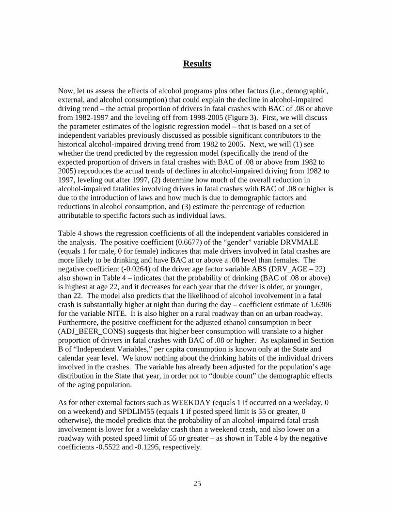
Table 1 Drivers With BAC = 08 or Greater in Fatal Crashes 1982-2005
Year
Drivers in Fatal Crashes
Total Percentage of Drivers With
BAC=08 or Greater
1982 56029 35 1983 54656 34 1984 57512 32 1985 57883 29 1986 60335 30 1987 61442 28 1988 62253 28 1989 60435 27 1990 58893 28 1991 54391 27 1992 51901 25 1993 53401 24 1994 54549 23 1995 56164 22 1996 57001 22 1997 56688 20 1998 56604 20 1999 56502 20 2000 57280 21 2001 57586 21 2002 58113 21 2003 58517 21 2004 58395 21 2005 59104 20
Source US Department of Transportation National Highway Traffic Safety Administration Traffic Safety Facts 2005
During the past two decades tireless efforts were made through national movements toward legislative enactments (BAC Illegal Per Se laws administrative licensing revocation (ALR) laws legal drinking age laws etc) to deter alcohol-impaired driving In addition many programs that were funded by States communities or private organizations were created to reduce alcohol-impaired driving These alcohol programs and laws served as a general deterrent to all those who drink and drive because they sent a message that the States were getting tougher on impaired driving and these efforts made people think twice about getting behind the wheel after they had been drinking In fact the trend of the proportion of crash fatalities that are alcohol-related ndash where BAC of
2
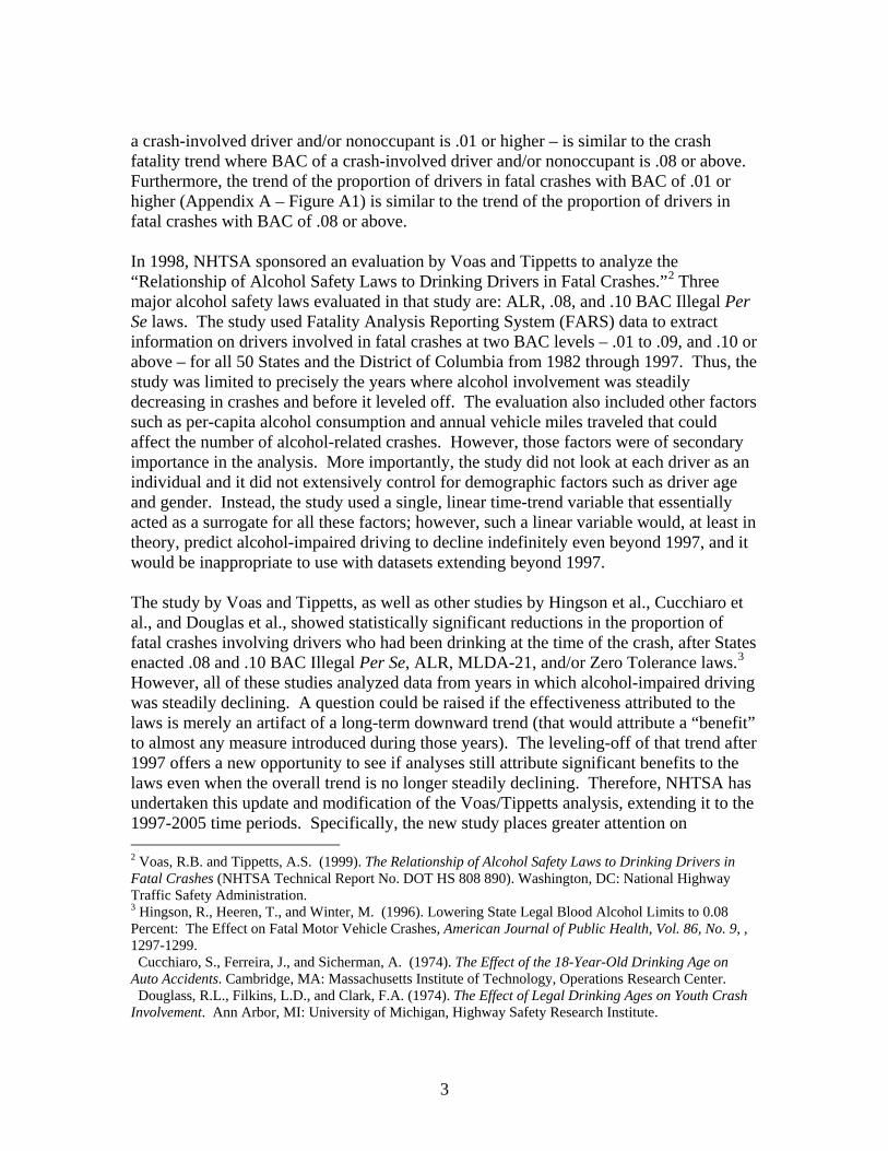
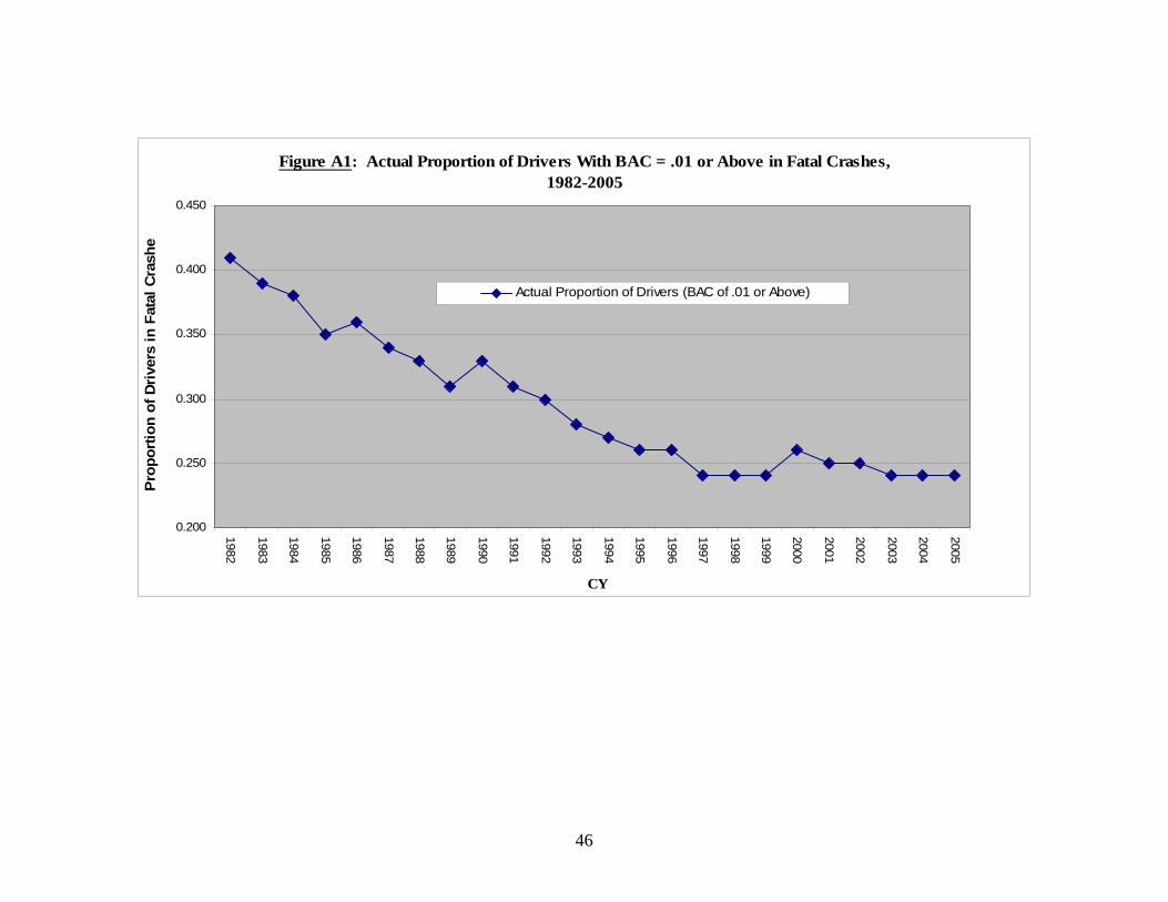
a crash-involved driver andor nonoccupant is 01 or higher ndash is similar to the crash fatality trend where BAC of a crash-involved driver andor nonoccupant is 08 or above Furthermore the trend of the proportion of drivers in fatal crashes with BAC of 01 or higher (Appendix A ndash Figure A1) is similar to the trend of the proportion of drivers in fatal crashes with BAC of 08 or above
In 1998 NHTSA sponsored an evaluation by Voas and Tippetts to analyze the ldquoRelationship of Alcohol Safety Laws to Drinking Drivers in Fatal Crashesrdquo2 Three major alcohol safety laws evaluated in that study are ALR 08 and 10 BAC Illegal Per Se laws The study used Fatality Analysis Reporting System (FARS) data to extract information on drivers involved in fatal crashes at two BAC levels ndash 01 to 09 and 10 or above ndash for all 50 States and the District of Columbia from 1982 through 1997 Thus the study was limited to precisely the years where alcohol involvement was steadily decreasing in crashes and before it leveled off The evaluation also included other factors such as per-capita alcohol consumption and annual vehicle miles traveled that could affect the number of alcohol-related crashes However those factors were of secondary importance in the analysis More importantly the study did not look at each driver as an individual and it did not extensively control for demographic factors such as driver age and gender Instead the study used a single linear time-trend variable that essentially acted as a surrogate for all these factors however such a linear variable would at least in theory predict alcohol-impaired driving to decline indefinitely even beyond 1997 and it would be inappropriate to use with datasets extending beyond 1997
The study by Voas and Tippetts as well as other studies by Hingson et al Cucchiaro et al and Douglas et al showed statistically significant reductions in the proportion of fatal crashes involving drivers who had been drinking at the time of the crash after States enacted 08 and 10 BAC Illegal Per Se ALR MLDA-21 andor Zero Tolerance laws3
However all of these studies analyzed data from years in which alcohol-impaired driving was steadily declining A question could be raised if the effectiveness attributed to the laws is merely an artifact of a long-term downward trend (that would attribute a ldquobenefitrdquo to almost any measure introduced during those years) The leveling-off of that trend after 1997 offers a new opportunity to see if analyses still attribute significant benefits to the laws even when the overall trend is no longer steadily declining Therefore NHTSA has undertaken this update and modification of the VoasTippetts analysis extending it to the 1997-2005 time periods Specifically the new study places greater attention on
2 Voas RB and Tippetts AS (1999) The Relationship of Alcohol Safety Laws to Drinking Drivers inFatal Crashes (NHTSA Technical Report No DOT HS 808 890) Washington DC National Highway Traffic Safety Administration3 Hingson R Heeren T and Winter M (1996) Lowering State Legal Blood Alcohol Limits to 008Percent The Effect on Fatal Motor Vehicle Crashes American Journal of Public Health Vol 86 No 9 1297-1299 Cucchiaro S Ferreira J and Sicherman A (1974) The Effect of the 18-Year-Old Drinking Age onAuto Accidents Cambridge MA Massachusetts Institute of Technology Operations Research Center Douglass RL Filkins LD and Clark FA (1974) The Effect of Legal Drinking Ages on Youth Crash Involvement Ann Arbor MI University of Michigan Highway Safety Research Institute
3
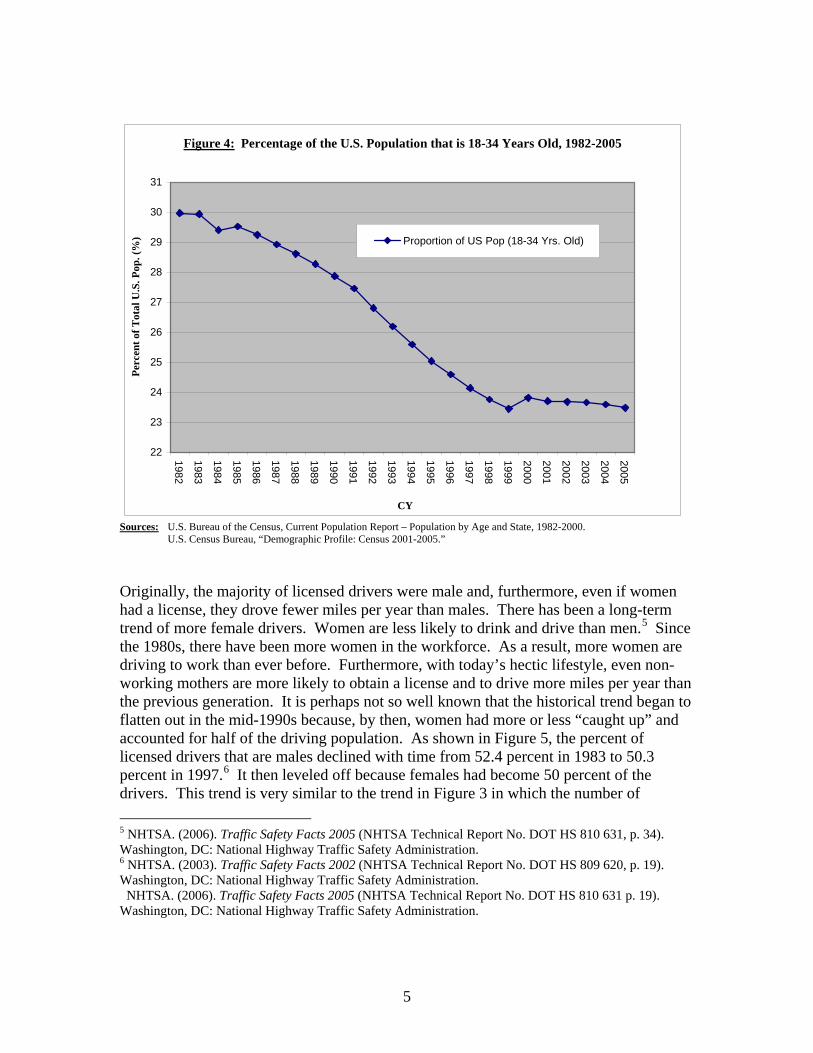
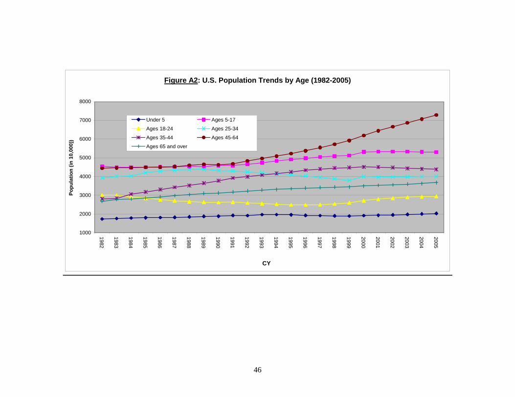
demographic as well as economic and other external factors that may have not only contributed to the steady decline in 1982-1997 but also influenced the post-1997 trend Critical factors include driver age gender and per-capita alcohol consumption Let us take a look at some of these factors to see how they might be possible contributors to the overall trend on alcohol-related fatalities in motor vehicle crashes It is known that the population of the United States has been steadily aging (Appendix A2) and that older people drink less But it is perhaps not so well known that the shrinkage has not been at a steady rate This is because the ldquobaby boomrdquo after World War II produced a bulge in the population distribution that aged with each passing year Figure 4 shows the percent of the United States population that is 18 to 34 years old4 The population age group (18 to 34 years old) shown in Figure 4 decreased at a steady rate from 1982 to 1999 and then gradually leveled off In 1982 the crest of the ldquobaby-boomersrdquo born in 1947 turned 35 and left their most intensive drinking years behind By 1999 the last of the baby-boomer generation born in 1960-1964 had reached 35 The trend in Figure 4 is not so different from the trend in alcohol-related fatalities (Figure 3) that leveled off after 1997 In other words here is one demographic factor that may partially explain both why the number of fatal crashes involving drivers who had been drinking progressively declined from 1982 to 1997 and why it gradually leveled off around that time
4 Current Population Reports ndash Resident Population By Age and State 1982-2005 Washington DC United States Census Bureau
4
Figure 4 Percentage of the US Population that is 18-34 Years Old 1982-2005
22
23
24
25
26
27
28
29
30
31
1982
1983
1984
1985
1986
1987
1988
1989
1990
1991
1992
1993
1994
1995
1996
1997
1998
1999
2000
2001
2002
2003
2004
2005
CY
Perc
ent o
f Tot
al U
S P
op (
) Proportion of US Pop (18-34 Yrs Old)
Sources US Bureau of the Census Current Population Report ndash Population by Age and State 1982-2000 US Census Bureau ldquoDemographic Profile Census 2001-2005rdquo
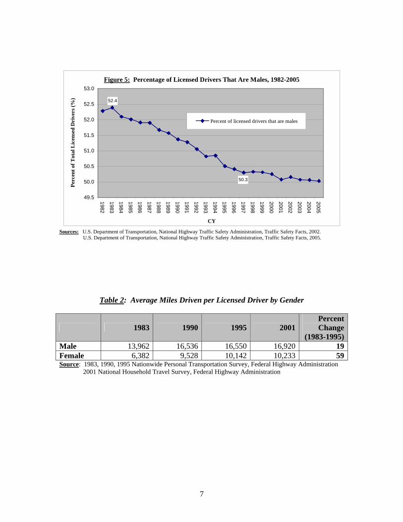
Originally the majority of licensed drivers were male and furthermore even if women had a license they drove fewer miles per year than males There has been a long-term trend of more female drivers Women are less likely to drink and drive than men5 Since the 1980s there have been more women in the workforce As a result more women are driving to work than ever before Furthermore with todayrsquos hectic lifestyle even non-working mothers are more likely to obtain a license and to drive more miles per year than the previous generation It is perhaps not so well known that the historical trend began to flatten out in the mid-1990s because by then women had more or less ldquocaught uprdquo and accounted for half of the driving population As shown in Figure 5 the percent of licensed drivers that are males declined with time from 524 percent in 1983 to 503 percent in 19976 It then leveled off because females had become 50 percent of the drivers This trend is very similar to the trend in Figure 3 in which the number of
5 NHTSA (2006) Traffic Safety Facts 2005 (NHTSA Technical Report No DOT HS 810 631 p 34)Washington DC National Highway Traffic Safety Administration6 NHTSA (2003) Traffic Safety Facts 2002 (NHTSA Technical Report No DOT HS 809 620 p 19)Washington DC National Highway Traffic Safety Administration
NHTSA (2006) Traffic Safety Facts 2005 (NHTSA Technical Report No DOT HS 810 631 p 19) Washington DC National Highway Traffic Safety Administration
5
fatalities involving drivers with BAC of 08 or above steadily declined and leveled off after 1997 Furthermore Table 2 shows the average annual miles per licensed driver by gender for calendar years 1983 1990 1995 and 2001 as well as the percent change from 1983 to 1995 Average annual miles per licensed driver increased 59 percent for women from 1983 to 1995 but only 19 percent for men The average annual miles driven did not change much from 1995 to 2001 for either men or women Although annual mileage is not available on a year-to-year basis here too it seems the trend is similar to Figure 3 with a leveling off somewhere in the mid-1990s Hence gender is another demographic factor that may influence the historical alcohol-related driving fatalities trend
Alcohol is an integral part of many Americansrsquo way of life Although the percentage of Americans who drink at all has not changed much in the last 30 years alcohol consumption per capita has declined quite a bit There is a widespread perception that the public has been placing more emphasis on health fitness and safety especially after 1980 In addition Federal State and local governments and private organizations have implemented many policies and programs to combat alcohol abuse One of the many actions taken by governments has been to increase the price of alcoholic beverages through tax increases However it is not clear as to whether the impact of tax hikes on alcohol consumption is significant since such increases at a wholesale level (ie by gallon barrel liter) are calculated to be negligible at a retail level after accounting for the effects of inflation Thus the increases would not strongly discourage light and moderate drinkers and certainly not alcohol abusers from purchasing alcohol
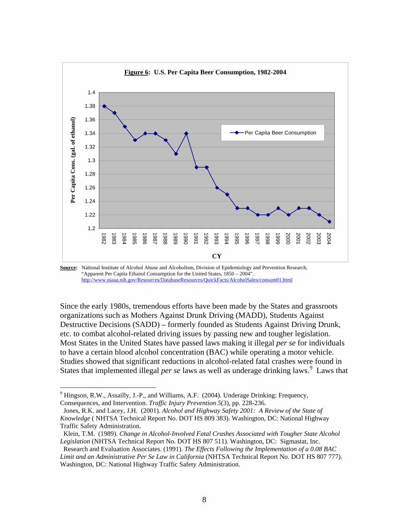
Figure 6 shows that the national per capita beer consumption (in gallons of ethanol) reduced from 138 in 1982 to 123 in 1995 and then leveled off (more or less)7 The trend in Figure 6 once again demonstrates similarity to the trend in Figure 3 According to Gallups annual Consumption Habits poll beer has always been the preferred alcoholic beverage for Americans since 19928 Hence beer consumption may further explain why the number of alcohol-related fatalities reduced over the fifteen-year period and why it has leveled off One contributing factor for the lowered beer consumption during this time period is that as previously discussed the ldquobaby boomrdquo generation is drinking less after they turn 35 and leave their drinking years behind Thus any analysis will need to adjust the trend in per capita consumption for changes in the age of the population Wine and liquor were neither included in the graph nor the regression analysis because (1) the initial analysis indicated that wine consumption was not significantly associated with the change in the alcohol-related driving trend ndash although there is a significant shift in wine preferences recorded by Gallup in the last eight years and in 2005 for the first time wine edged out beer as the standard drink for most Americans and (2) liquor has consistently ranked third as the preferred drink behind wine and beer
7 Apparent Per Capita Ethanol Consumption for the United States 1850-2004 accessible fromwwwniaaanihgovdatabasesqfhtmcons8 Jones J (July 31 2006) US Drinkers Consuming Alcohol More Regularly ndash Beer Regains Slight Edge Over Wine as Preferred Drink The Gallup Poll News Service Washington DC
6
Figure 5 Percentage of Licensed Drivers That Are Males 1982-2005
503
524
495
500
505
510
515
520
525
530
Percent of licensed drivers that are males
2005
2004
2003
2002
2001
2000
1999
1998
1997
1996
1995
1994
1993
1992
1991
1990
1989
1988
1987
1986
1985
1984
1983
1982
CY
Sources US Department of Transportation National Highway Traffic Safety Administration Traffic Safety Facts 2002 US Department of Transportation National Highway Traffic Safety Administration Traffic Safety Facts 2005
Perc
ent o
f Tot
al L
icen
sed
Dri
vers
()
Table 2 Average Miles Driven per Licensed Driver by Gender
1983 1990 1995 2001 Percent Change
(1983-1995) Male 13962 16536 16550 16920 19 Female 6382 9528 10142 10233 59 Source 1983 1990 1995 Nationwide Personal Transportation Survey Federal Highway Administration
2001 National Household Travel Survey Federal Highway Administration
7
Figure 6 US Per Capita Beer Consumption 1982-2004
12
122
124
126
128
13
132
134
136
138
14
1982
1983
1984
1985
1986
1987
1988
1989
1990
1991
1992
1993
1994
1995
1996
1997
1998
1999
2000
2001
2002
2003
2004
CY
Per
Cap
ita C
ons
(gal
of e
than
ol)
Per Capita Beer Consumption
Source National Institute of Alcohol Abuse and Alcoholism Division of Epidemiology and Prevention Research ldquoApparent Per Capita Ethanol Consumption for the United States 1850 ndash 2004rdquo
httpwwwniaaanihgovResourcesDatabaseResourcesQuickFactsAlcoholSalesconsum01html
Since the early 1980s tremendous efforts have been made by the States and grassroots organizations such as Mothers Against Drunk Driving (MADD) Students Against Destructive Decisions (SADD) ndash formerly founded as Students Against Driving Drunk etc to combat alcohol-related driving issues by passing new and tougher legislation Most States in the United States have passed laws making it illegal per se for individuals to have a certain blood alcohol concentration (BAC) while operating a motor vehicle Studies showed that significant reductions in alcohol-related fatal crashes were found in States that implemented illegal per se laws as well as underage drinking laws9 Laws that
9 Hingson RW Assailly J-P and Williams AF (2004) Underage Drinking Frequency Consequences and Intervention Traffic Injury Prevention 5(3) pp 228-236 Jones RK and Lacey JH (2001) Alcohol and Highway Safety 2001 A Review of the State of Knowledge ( NHTSA Technical Report No DOT HS 809 383) Washington DC National Highway Traffic Safety Administration Klein TM (1989) Change in Alcohol-Involved Fatal Crashes Associated with Tougher State Alcohol Legislation (NHTSA Technical Report No DOT HS 807 511) Washington DC Sigmastat Inc Research and Evaluation Associates (1991) The Effects Following the Implementation of a 008 BAC Limit and an Administrative Per Se Law in California (NHTSA Technical Report No DOT HS 807 777) Washington DC National Highway Traffic Safety Administration
8
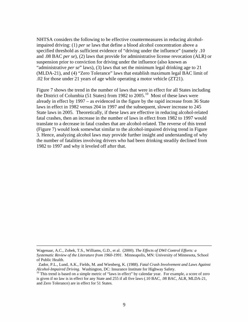
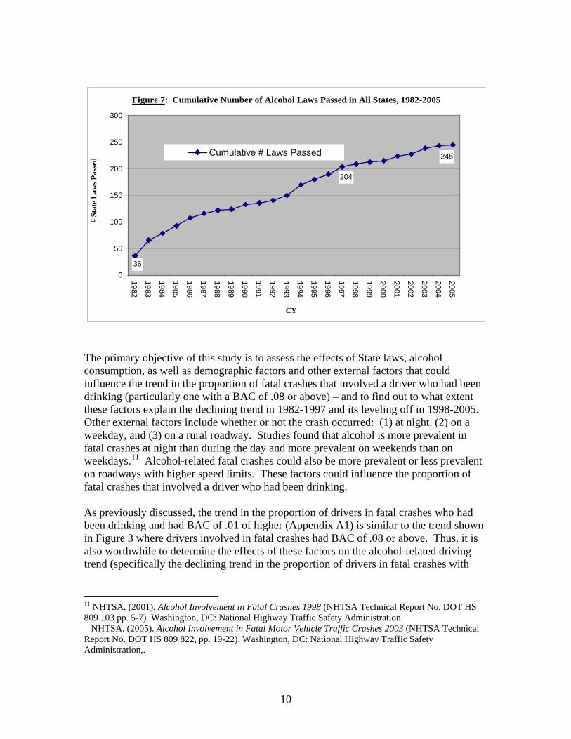
NHTSA considers the following to be effective countermeasures in reducing alcohol-impaired driving (1) per se laws that define a blood alcohol concentration above a specified threshold as sufficient evidence of ldquodriving under the influencerdquo (namely 10 and 08 BAC per se) (2) laws that provide for administrative license revocation (ALR) or suspension prior to conviction for driving under the influence (also known as ldquoadministrative per serdquo laws) (3) laws that set the minimum legal drinking age to 21 (MLDA-21) and (4) ldquoZero Tolerancerdquo laws that establish maximum legal BAC limit of 02 for those under 21 years of age while operating a motor vehicle (ZT21)
Figure 7 shows the trend in the number of laws that were in effect for all States including the District of Columbia (51 States) from 1982 to 200510 Most of these laws were already in effect by 1997 ndash as evidenced in the figure by the rapid increase from 36 State laws in effect in 1982 versus 204 in 1997 and the subsequent slower increase to 245 State laws in 2005 Theoretically if these laws are effective in reducing alcohol-related fatal crashes then an increase in the number of laws in effect from 1982 to 1997 would translate to a decrease in fatal crashes that are alcohol-related The reverse of this trend (Figure 7) would look somewhat similar to the alcohol-impaired driving trend in Figure 3 Hence analyzing alcohol laws may provide further insight and understanding of why the number of fatalities involving drivers who had been drinking steadily declined from 1982 to 1997 and why it leveled off after that
Wagenaar AC Zobek TS Williams GD et al (2000) The Effects of DWI Control Efforts a Systematic Review of the Literature from 1960-1991 Minneapolis MN University of Minnesota School of Public Health
Zador PL Lund AK Fields M and Wienberg K (1988) Fatal Crash Involvement and Laws Against Alcohol-Impaired Driving Washington DC Insurance Institute for Highway Safety 10 This trend is based on a simple metric of ldquolaws in effectrdquo by calendar year For example a score of zero is given if no law is in effect for any State and 255 if all five laws (10 BAC 08 BAC ALR MLDA-21 and Zero Tolerance) are in effect for 51 States
9
St
ate
Law
s Pas
sed
300
250
200
150
100
50
0
Figure 7 Cumulative Number of Alcohol Laws Passed in All States 1982-2005
36
204
245Cumulative Laws Passed
2005
2004
2003
2002
2001
2000
1999
1998
1997
1996
1995
1994
1993
1992
1991
1990
1989
1988
1987
1986
1985
1984
1983
1982
CY
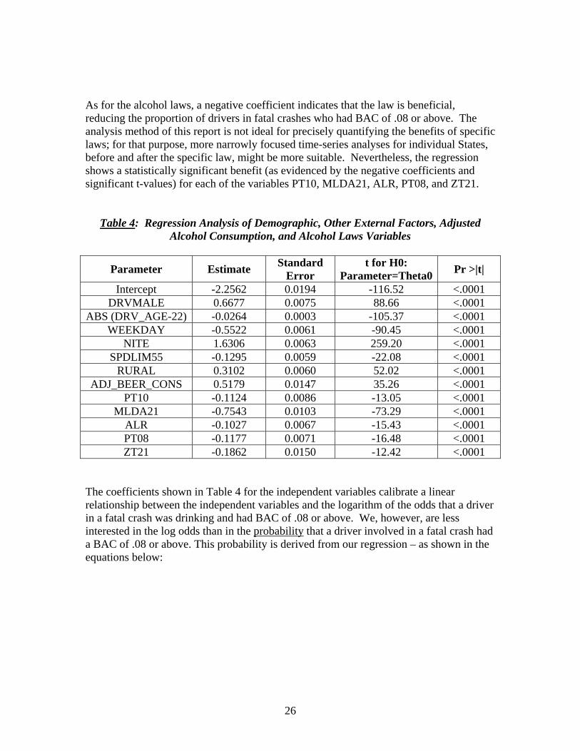
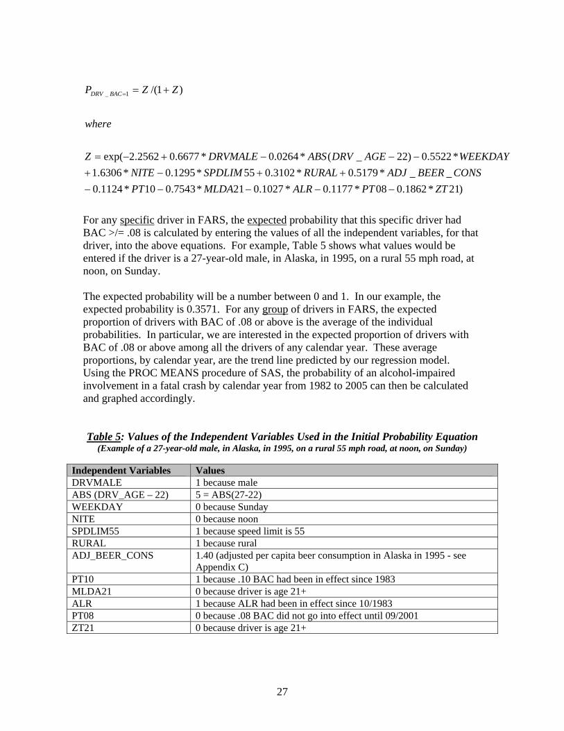
The primary objective of this study is to assess the effects of State laws alcohol consumption as well as demographic factors and other external factors that could influence the trend in the proportion of fatal crashes that involved a driver who had been drinking (particularly one with a BAC of 08 or above) ndash and to find out to what extent these factors explain the declining trend in 1982-1997 and its leveling off in 1998-2005 Other external factors include whether or not the crash occurred (1) at night (2) on a weekday and (3) on a rural roadway Studies found that alcohol is more prevalent in fatal crashes at night than during the day and more prevalent on weekends than on weekdays11 Alcohol-related fatal crashes could also be more prevalent or less prevalent on roadways with higher speed limits These factors could influence the proportion of fatal crashes that involved a driver who had been drinking
As previously discussed the trend in the proportion of drivers in fatal crashes who had been drinking and had BAC of 01 of higher (Appendix A1) is similar to the trend shown in Figure 3 where drivers involved in fatal crashes had BAC of 08 or above Thus it is also worthwhile to determine the effects of these factors on the alcohol-related driving trend (specifically the declining trend in the proportion of drivers in fatal crashes with
11 NHTSA (2001) Alcohol Involvement in Fatal Crashes 1998 (NHTSA Technical Report No DOT HS 809 103 pp 5-7) Washington DC National Highway Traffic Safety Administration
NHTSA (2005) Alcohol Involvement in Fatal Motor Vehicle Traffic Crashes 2003 (NHTSA Technical Report No DOT HS 809 822 pp 19-22) Washington DC National Highway Traffic Safety Administration
10
BAC of 01 or above from 1982 to 1997 and the leveling off after 1997) and to what extent these factors explain the trend
The principal analytic tool will be logistic regressions of the probability that a driver involved in a fatal crash had been drinking Logistic regression allows us to analyze each driver as a separate entity taking into account the driverrsquos age and gender In addition we can take into account (1) what laws were in effect on the day of the crash and (2) the conditions under which alcohol-related fatal crashes are particularly prevalent
11
Method
In their 1998 analysis Voas and Tippetts used Kleinrsquos imputation method which was the method being used in FARS at the time of the study to estimate the BAC of drivers in fatal crashes where alcohol test results were unknown For those drivers Kleinrsquos technique would calculate the probability that those drivers had a BAC in grams per deciliter (gdL) of 00 01 to 09 or 10 and above12 As a result Voas and Tippetts were able to analyze all drivers in fatal crashes at two different BAC levels (01 to 09 and 10 or above) since both the imputed and known BAC data are available in all 50 States and the District of Columbia
Multiple Imputation Method
Currently the multiple imputation method is being used in FARS for the same purpose13
Hence the multiple imputation method for handling missing BAC values was used for all the FARS data (1982-2005) included in this analysis The difference between the two methods is that the multiple imputation method imputes ten values of BAC for each missing BAC value whereas Kleinrsquos method calculates the probability that a missing BAC value falls within one of the three ranges (00 01-09 or 10 and above) The advantage of using the current method is that it allows the computation of statistics such as variances measures of central tendency confidence intervals and standard deviations With the current procedure each missing BAC value is replaced with ten simulated values14 However if the actual BAC is measured and known all ten values are set to the actual value The ten imputations along with the actual BAC values will first generate ten sets of BAC values (ie ten matrices) each of which will then be analyzed separately The variation obtained from analyzing the ten sets of values will be used to calculate estimates of error attributed to the imputation process Results from each of the ten sets of BAC values will then be combined by a procedure specified by Rubin to (1) estimate quantities of interest (eg proportion of drivers involved in fatal crashes with BAC of 08 or greater) and (2) produce statistical inferences that are valid (eg consistent estimation of parameters accurate calculation of 95 percent confidence intervals etc)15
12 Klein T (1986) A Method for Estimating Posterior BAC Distributions for Persons Involved in Fatal Traffic Accidents ( NHTSA Technical Report No DOT HS 807 094) Washington DC National HighwayTraffic Safety Administration 13 Subramanian R (2002) Transitioning to Multiple Imputation ndash A New Method to Impute Missing BloodAlcohol Concentration (BAC) Values in FARS (NHTSA Technical Report No DOT HS 809 403) Washington DC National Highway Traffic Safety Administration 14 The imputed values are actual values of BAC along the entire plausible range and can therefore becombined to provide estimates for any defined category of alcohol involvement (ie BAC=01+ BAC=08 BAC08+ etc) 15 Rubin D (1987) Multiple Imputation of Nonresponse in Surveys J Wiley and Sons New York
12
Dependent variable
In estimating the extent of alcohol involvement in fatal crashes one quantity of interest is the proportion of drivers who were drinking involved in fatal crashes Many factors that affect fatal crashes are likely to have a similar effect on both non-alcohol and alcohol-related fatal crashes For their dependent variable Voas and Tippetts used the ratio of drivers in fatal crashes with positive BAC test results to drivers in crashes with zero BAC results Use of this dependent variable automatically controls for factors that have similar influences on all crashes This study will use essentially the same dependent variable ndash DRV_BAC This dependent variable will have a value of 1 for drivers with imputed or known BAC values of 08 and greater and a value of 2 for all other drivers Logistic regression will be used to calibrate the odds that DRV_BAC = 1 ndash ie the odds that a driver involved in a fatal crash was drinking and had BAC of 08 or above
Independent variables
As discussed in the previous chapter ldquoMotivation for This Studyrdquo control factors such as driver age gender external factors per-capita alcohol consumption as well as alcohol-related legislation are all possible contributors to the overall alcohol-related driving trend Demographic and external variables will be discussed first followed by detailed discussion of the alcohol consumption and programmatic variables The following independent variables are obtained directly from FARS or defined for the purpose of the study
A) Demographic and external variables
bull Gender expressed as DRVMALE (=1 if the driver is male and 0 if the driver is female)
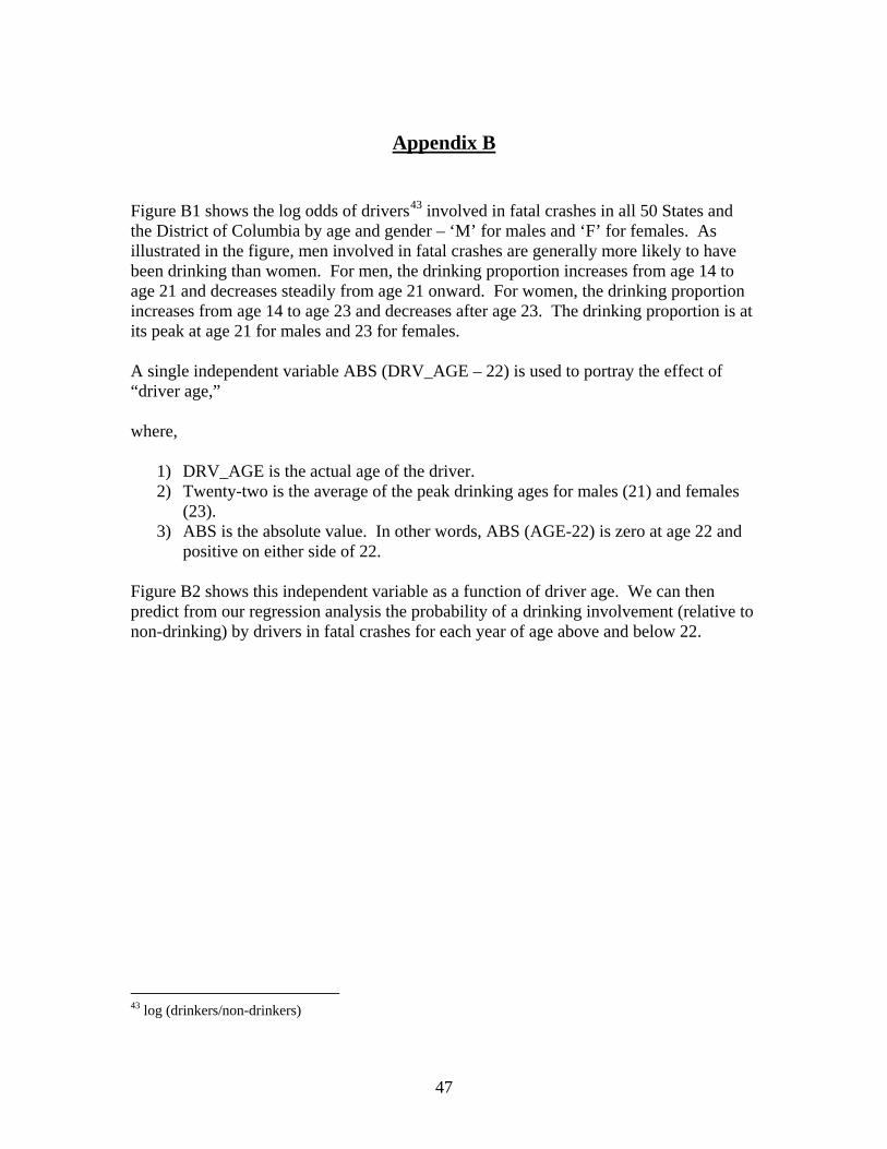
bull The driverrsquos age expressed as ABS(DRV_AGE-22)16 where 1) ABS is the absolute value 2) 22 is the average driverrsquos age for both males and females with the highest
proportion of drivers in fatal crashes who had a BAC of 08 or above 3) DRV_AGE is the actual age of the driver
bull Day of the week expressed as WEEKDAY (=1 if the crash occurred on a Monday Tuesday Wednesday Thursday or Friday and 0 if on a Saturday or Sunday)
bull Time of day expressed as NITE (=1 if 7 pm ndash 559 am 0 if 6 am ndash 659 pm)
16 Refer to Appendix B for a detailed explanation of the derived formula
13
bull Roadway function class expressed as RURAL (= 1 if the crash occurred on a rural roadway and 0 if the crash occurred on an urban roadway)
bull Posted speed limit expressed as SPDLIM55 (=1 if the posted speed limit is 55 ndash 75 miles per hour (mph) and 0 if 5 ndash 50 mph)
In this analysis the dependent variable was modeled as a function of several demographic and external variables Some of these variables had also been used in deriving the imputed BAC values in FARS Let us briefly discuss the interrelationships between the model used for imputation and the model used for regression analysis It is necessary to choose an imputation model that is compatible with the analyses to be performed on the imputed datasets hence the imputation model must be robust enough to preserve the associations among variables that will be used later in the investigation17
Thus there is no need to include the same variables in the latter model since they had already been used in the imputation model ndash unless their relationships to the dependent variable are of considerable interest ndash which in this analysis the demographic and certain external variables are factors that may influence the historical alcohol-related driving fatalities trend Results pertaining to the dependent variable are not biased by the inclusion of the same variables in the regression model
B) Adjusted per capita alcohol consumption
As discussed earlier for the past 20 years the trend of the national per capita alcohol consumption ndash specifically beer consumption ndash somewhat mirrors the national alcohol-impaired driving trend This study will look at per capita ethanol consumption for beer by State and calendar year ndash to analyze its effects in reducing crash fatalities that involved drivers with a BAC of 08 or above The national and State per capita ethanol consumption data are obtained from the National Institute of Alcohol Abuse and Alcoholism and computed for the entire population (all age groups)18 In reality alcohol consumption differs significantly due to demographic as well as behavioral changes in the population In other words if the population ages over time or if a State has an older-than-average population that will lower the overall alcohol consumption even if consumption stays the same in each age cohort Thus consumption data will have to be adjusted in the analysis to reflect different consumption levels by age group by year and by State Specifically the 1982-1997 downward trend in actual consumption (Figure 6) is partly due to the aging of the population and it overstates the actual reduction in consumption for say 30-year-olds due to purely behavioral change Appendix C will discuss in detail the calculation of the adjusted per capita alcohol consumption by State and by year
17 Rubin DB (1996) Multiple Imputation After 18+ Years (With Discussion) Journal of the American Statistical Association 91 473-489 18 Per Capita Ethanol Consumption for States Census Regions and the United States 1970-2003 accessible from wwwniaaanihgovdatabasesqfhtmcons
14
C) Programmatic independent variables Alcohol-related legislation
During the past two decades many programs were created and laws passed to deter alcohol-impaired driving In this study we will look at particularly the passage of the Illegal Per Se ALR and drinking age laws to 1) study the immediate effects that these laws had on the general population and 2) explain how they impact the historical alcohol-impaired driving trend
Let us first discuss in detail each of the laws by 1) defining its function 2) providing some background information (ie legislation efforts enactment status etc) and 3) presenting findings from other studies on the effectiveness of these laws A separate section identifying the variables (representing the laws) will then follow
Background information on alcohol laws
In the early 1980s approximately three-fourths of the States had passed what are now known as 10 BAC Illegal Per Se laws and by the mid 1990s all but two States Massachusetts and South Carolina had adopted such laws19 These laws make it illegal for an individual to operate a motor vehicle at or above 10 BAC essentially making a BAC of 10 or above sufficient evidence that a person was ldquodriving under the influencerdquo During this period the number of alcohol-impaired fatalities had dropped by 15 percent or more (Figure 3) In 1989 Kleinrsquos study concluded that 6 out of 26 States which implemented the per se laws experienced significant reductions in the alcohol-impaired driving fatality rate Most of these States had the 10 BAC limit20 However many research and epidemiologic findings suggested that a BAC limit of 10 was too lenient and that 08 was a more effective threshold Utah Oregon and Maine were the only three States in the 1980s to reduce their BAC threshold to 08 Great Britain other countries in Europe and Australia experienced significant declines in drinking and driving where the BAC limits were set at 08 or 0521 Dennis et al conducted an experiment to study the effect of alcohol on individualsrsquo driving abilities by evaluating their handling judgment and decision making at various BAC levels (00 03 07 and 11)22 The results showed a decline in reaction time at a BAC of 11 and progressive declines in both glare recovery time and driving ability as BAC increases Hingson et al reported significant reductions in the proportion of fatal crashes involving drivers with
19 Voas RB and Tippetts AS (1999) The Relationship of Alcohol Safety Laws to Drinking Drivers in Fatal Crashes (NHTSA Technical Report Number DOT HS 808 890 p7) Washington DC National Highway Traffic Safety Administration 20 Klein TM (1989) Changes in Alcohol-Involved Fatal Crashes Associated with Tougher State Alcohol Legislation (NHTSA Technical Report No DOT HS 807 094) Washington DC Sigmastat Inc 21 Stewart K (2000) On DWI Laws in Other Countries (NHTSA Report No DOT HS 809 037) Washington DC National Highway Traffic Safety 22 Dennis ME (1995) Effects of Alcohol on Driving Task Abilities American Drivers and Traffic Safety Education Association ndash The Chronology Summer Issue Indiana PA
15
BAC above 08 when he compared five States that had adopted the 08 threshold with five neighboring States that had kept the 10 threshold23 The strong relationships between BAC levels increased impairment and probability of crash involvement have convinced many States to lower their legal BAC limitslowast In 2001 the Centers for Disease Control performed a review of the available literature and concluded that the 08 BAC law reduced alcohol-related fatalities by an average of 7 percent24 Currently all 50 States and the District of Columbia have adopted the 08 threshold25
When coupled with a 08 Illegal Per Se law administrative license revocation (ALR) sanctions have proven to be one of the most effective ways to deter alcohol-impaired driving ALR allows police officers to seize the driverrsquos license of individuals who failed a BAC test or refused to submit to a test Currently 41 States and the District of Columbia have adopted some form of administrative license revocation26 NHTSA conducted a study in California to determine the effect of implementing 08 Illegal Per Se and ALR laws on alcohol-related fatalities and found a 12-percent reduction when California passed both laws27 Another NHTSA study reported that Illinois New Mexico Maine North Carolina Colorado and Utah experienced significant reductions in alcohol-related fatal crashes after the passage of the ALR law in those States28 In an independent study for the Insurance Institute for Highway Safety researchers found that the number of alcohol involved nighttime fatal crashes was reduced by 9 percent in States that adopted an ALR law relative to States that had not adopted such laws29 It is believed that ALR not only deterred potential offenders but also deterred convictedrepeat offenders due to its swiftness and certainty One study found that the recidivism rates decreased by 10 percentage points (15 to 5) for first time offenders and by 18 percentage points (25 to 7) for multiple offenders30
After the repeal of Prohibition in an effort to restrict youth access to alcohol nearly all States designated 21 as the minimum legal drinking age (MLDA) Then from 1970 to 1975 29 States lowered the MLDA to 17 18 19 or 2031 During this period numerous
23 Hingson R Heereen T and Winter M (1996) Lowering State Legal Blood Alcohol Limits to 08 Percent The Effect on Fatal Motor Vehicle Crashes American Journal of Public Health 86(9) September lowast These noted studies are only examples of the many studies on impairment at various BAC levels and onthe effectiveness of 08 BAC laws 24 Effectiveness of 008 Percent Blood Alcohol Concentration (BAC) Laws CDC Community Guide 2001 25 NHTSA (2005) Traffic Safety LawsFacts Office of Program Development amp Delivery 26 NHTSA (2005) Traffic Safety LawsFacts Office of Program Development amp Delivery 27 NHTSA (1991) The Effects Following the Implementation of a 008 BAC Limit and an Administrative Per Se Law in California (NHTSA Report No DOT HS 807 777) Washington DC National HighwayTraffic Safety Administration28 NHTSA (1996) State Legislative Fact Sheet 29 Zador PL Lund AK Fields M and Weinberg K (1989) Fatal Crash Involvement and LawsAgainst Alcohol-Impaired Driving Washington DC Insurance Institute for Highway Safety 30 Voas RB Tippetts AS and Taylor EP (1999) Impact of Ohio Administrative License Suspension Journal of Crash Prevention and Injury Control 31 The Minimum Legal Drinking Age Facts and Fallacies accessible from wwwama-assnorgamapubarticle3566-3640html
16
research findings indicated that motor vehicle crashes the leading cause of death among teenagers increased significantly in States where MLDA was lowered32 Armed with such strong evidence (from many studies) linking lower drinking age laws with higher motor vehicle fatalities among youths 16 States restored their MLDA to 21 between 1976 and 1983 The National Minimum Drinking Age Act of 1984 required all States to raise their minimum purchase and public possession of alcohol age to 21 The Federal Aid Highway Act mandated a reduction of Federal transportation funds to States that had not raised the MLDA to 21 By January 1988 every State had adopted 21 as the MLDA In 1982 55 percent of all fatal crashes involving young drivers were alcohol-related when many of the States had minimum drinking ages of 18 Since the National Minimum Drinking Age Act of 1984 the alcohol-related traffic fatality rate has been reduced by half
The MLDA-21 law was given much credit for the decrease of youth drinking and driving by reducing the availability of alcohol and by establishing the threat of punishment for alcohol use A subsequent law that further increases the deterrent effect on youth drinking and driving was the Zero Tolerance law This law makes it illegal for drivers under the age of 21 to operate a motor vehicle with a BAC of 02 or more Violators of such law have their driverrsquos license suspended or revoked By 1998 all States and the District of Columbia had adopted this law In the mid 1990s Hingson et al compared 12 States that had enacted the Zero Tolerance law with 12 neighboring States that had not enacted such law in a given prepost law period and found that single vehicle nighttime crashes among young drivers dropped 16 percent in the zero tolerance States while the neighboring States had a 1 percent increase33 An early study in Maryland found that alcohol-related crashes for young drivers (ages 21 or less) decreased by 21 percent in six counties after the Zero Tolerance law was implemented34
32 Cucchiaro S Ferreira J and Sicherman A (1974) The Effect of the 18-Year-Old Drinking Age on Auto Accidents Cambridge MA Massachusetts Institute of Technology Operations Research Center
Douglass RL Filkins LD and Clark FA (1974) The Effect of Legal Drinking Ages on Youth Crash Involvement Ann Arbor MI University of Michigan Highway Safety Research Institute
Williams AF Rich RF Zador PL and Robertson LS (1974) The Legal Minimum Drinking Age and Fatal Motor Vehicle Crashes Washington DC Insurance Institute for Highway Safety
33 Hingson RW et al (1994) Lower Legal Blood Alcohol Limits for YoungDrivers Public Health Reports 34 Jones RK and Lacey JH (2001) Alcohol and Highway Safety 2001 A Review of the State of Knowledge (NHTSA Technical Report No DOT HS 809 383) Washington DC National Highway Traffic Safety Administration
17
Defining variables for the laws
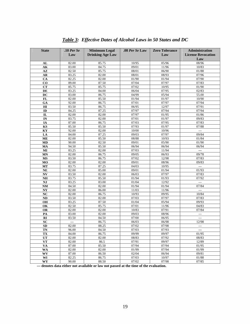
Table 3 lists the effective dates of the five laws in 50 States and the District of Columbia35 The effective dates are not themselves independent variables in the analysis but are used to define the independent variables36
The per se laws and ALR laws apply to drivers of all ages An independent variable PT10 is defined to be
0 if no per se law was in effect on the date of the crash in the State where the crash occurred
1 if a per se law for BAC 10 or lower was in effect on the date of the crash in that State
Similarly an independent variable PT08 is defined to be
0 if no per se law at all or only a BAC 10 law was in effect on the date of the crash in the State where the crash occurred
1 if a BAC 08 law was in effect on the date of the crash in that State
The variable ALR is defined to be zero if ALR was not in effect in that State on the day of the crash 1 if it was in effect
MLDA-21 and Zero Tolerance laws only apply to drivers under the age of 21 Thus the independent variable MLDA21 is defined to be
0 for any driver age 21 or older 0 for drivers under 21 if the minimum legal drinking age was not 21 on the date
of the crash in the State where the crash occurred 1 for drivers under 21 if the minimum legal drinking age was 21 on the date of
the crash in that State
The variable ZT21 is defined to be 1 for drivers under age 21 if the Zero Tolerance law was in effect in that State on the day of the crash 0 for all other drivers
Once the dependent and independent variables were defined in the SAS datasets the next steps were to combine the datasets including the imputed BAC values and perform logistic regression analysis The next several sections discuss in detail the coding analysis procedure
35 Tippetts AS Pacific Institute for Research and Evaluation an Excel spreadsheet e-mailed to Jennifer Dang on 080103 36 Refer to Appendix D for a detailed explanation of how the variables for the laws were defined
18
Table 3 Effective Dates of Alcohol Laws in 50 States and DC
State 10 Per Se Law
Minimum Legal Drinking Age Law
08 Per Se Law Zero Tolerance Law
Administration License Revocation
Law AL 8200 8575 1095 0596 0896 AK 8300 8475 0901 1196 1083 AZ 8250 8575 0801 0690 0188 AR 8325 8200 0801 0893 0796 CA 8225 8200 0190 0194 0790 CO 8900 8750 0704 0797 0783 CT 8575 8575 0702 1095 0190 DE 8325 8400 0604 0795 0283 DC 8300 8675 0499 0594 5500 FL 8200 8550 0194 0197 1090 GA 9200 8675 0701 0797 0794 HI 8350 8675 0695 1297 0791 ID 8425 8725 0797 0794 0794 IL 8200 8200 0797 0195 0186 IN 8375 8200 0701 0197 0983 IA 8700 8675 0703 0795 0783 KS 8550 8550 0793 0197 0788 KY 9200 8200 1000 1096 --- LA 8400 8725 0903 0797 0984 ME 8200 8550 0888 1093 0184 MD 9000 8250 0901 0590 0190 MA 9450 8550 0694 0694 0694 MI 8325 8200 0703 1194 --- MN 8200 8675 0905 0693 0978 MS 8350 8675 0702 1298 0783 MO 8200 8200 0901 0896 0983 MT 8375 8725 0403 1095 --- NE 8200 8500 0901 0194 0193 NV 8350 8200 0603 0797 0783 NH 8375 8550 0194 0193 0792 NJ 8325 8300 0104 1292 --- NM 8450 8200 0194 0194 0784 NY 8200 8600 1103 1196 --- NC 8200 8675 1093 0995 1084 ND 8350 8200 0703 0797 0783 OH 8325 8750 0104 0594 0993 OK 8250 8575 0701 1196 0483 OR 8200 8200 1083 0791 0784 PA 8300 8200 0903 0896 --- RI 8350 8450 0700 0695 --- SC --- 8675 0603 0698 1298 SD 8200 8825 0702 0798 --- TN 9600 8450 0703 0793 --- TX 8400 8675 0999 0997 0195 UT 8200 8200 0883 0792 0883 VT 8200 865 0791 0997 1289 VA 8700 8550 0794 0794 0195 WA 8200 8200 0199 0794 0199 WV 8700 8650 0204 0694 0981 WI 8225 8675 0703 1097 0188 WY 9000 8850 0702 0798 0785
--- denotes data either not available or law not passed at the time of the evaluation
19
D) Other potential independent variables
We surveyed the literature and where possible performed exploratory analyses with other factors that might have significantly reduced alcohol involvement in fatal crashes
bull Activism of non-government organizations such as MADD and SADD has undoubtedly made the public more aware and less tolerant of the alcohol-impaired driving problem by educating them on crash and injury risks posed by drinking and driving and on the effects of alcohol use and abuse MADD created the first two chapters in California and Maryland in 1980 and grew to 100 chapters in 1982 to 300 chapters in 47 States in 198437 Likewise SADD was founded in Massachusetts in 1981 and created hundreds of chapters throughout nine States in 1982 and many more thereafter38 Moreover telemarketing programs and other organizations that supported the growth and development of these organizational chapters across the country have promoted tremendous awareness to the general public across all ages of the alcohol-impaired driving issues Thus these organizations contributed to the reduction in alcohol-impaired driving in the early 1980s ndash specifically in 1982-1985 These public information programs and education have (1) provided support and momentum for passing alcohol legislation (2) increased deterrent effect by educating the public on the provisions and penalties of the laws and (3) generated public support for law enforcement programs However when we investigated quantifying this factor for the analysis (ie by counting the number of MADD and SADD chapters by year and by State) we found such information was not readily available
bull Enforcement is obviously an important factor in deterring alcohol-impaired driving The only quantitative information (by year and State) available to us was the DUI arrest data obtained from the Uniform Crime Reports published yearly by the Federal Bureau of Investigation39 The absolute number of arrests however may be an indication of the size of the underlying problem as well as the level of enforcement More arrests could mean there are more drinkers or that enforcement was intensified The number of arrests should be measured relative to the size of the drinking problem
Aggregate national data initially suggested this could be a promising variable During the critical years 1982-85 nationwide arrests went up while drunk-driving fatalities sharply decreased suggesting a trend of stricter enforcement That encouraged us to define an arrest index for each State and year normalizing the
37 httpwwwmaddorgaboutus11056117900html 38 httpwwwsaddonlinecomhistoryhtm 39 httpwwwfbigovucrcius2006datatable_69html
20
arrests alcohol _ consumption given _ year
⎛⎜⎝ ⎡ ⎤
arrests
⎞⎟⎠
alcohol consumption
⎢ ⎢ ⎢ ⎢⎣
⎥ ⎥ ⎥ ⎥⎦
Arrest index_ =100 given year ⎛⎜⎝
⎞⎟⎠1982
_
_
bull
bull
bull
bull
bull httpwwwbeagovregionalgspactioncfm
number of arrests relative to aggregate alcohol consumption and enter it in our model The arrest index is defined as follows
However this independent variable did not have a statistically significant correlation with alcohol-related driving fatalities across our database
Sobriety checkpoints also act as deterrents to drivers who drink and remind them and the general public that alcohol-impaired driving is not only socially unacceptable but also a crime When adequately publicized they can be very effective Most States allow sobriety checkpoints and many States set their own guidelines but still comply with the Federal requirements Only information such as the year that the States initially permitted sobriety checkpoints was available We entered that variable in our analysis as another possible measure of enforcement levels However it did not have a statistically significant association with our dependent variable
Although enforcement and activism (MADD SADD) could not be directly included as variables in the model it could be argued that their effect is implicitly present Parts of the fatality reductions that the model attributes to the various laws is a consequence of the enforcement and publicity activities that have made the laws effective
The economy could play a role in the reduction of alcohol-impaired driving where an economic slowdown might after a while lead to reduced partying and alcohol consumption while a resumption of growth could initially increase non-drinking fatalities (work- and shopping-related) lowering the ratio of drinkers to non-drinkers We obtained a measure of economic activity by State and yearbull ndash the Gross State Product per capita ndash from the Bureau of Economic Analysis and included it in our model However neither this variable nor permutations of it such as a 1-year or 2-year lag had a significant correlation with our dependent variable
Increasing taxes on alcohol could reduce alcohol-impaired driving by discouraging alcohol consumption directly by increasing its price and indirectly by fostering a societal attitude against excessive consumption It is true that the
21
Federal tax on beer was doubled from $9 to $18 per 31-gallon barrel in 1991 However that amounts to an increase of less than 3 cents per 12-ounce serving It is unlikely that an increase of 3 cents per can or bottle had much of an effect on drinking and driving Moreover to the extent that increased price directly reduces consumption its effect is already included in our per capita consumption variable
bull One other important safety legislation that was not analyzed in this study is the seat belt laws The relationship between these laws and drivers in alcohol-related fatal crashes is complex Historically drivers who had been drinking at the time of the crash have always had lower belt use than drivers who had not However information on belt use by year and by State was not readily available
Analyzing the multiple-imputed datasets in FARS
The Multiple Imputation database available at NHTSA and used in this study includes for each specific driver case on FARS with missing values of BAC ten predictions of that BAC based on the non-missing values of other FARS variables for that driver and crash such as the driverrsquos age and gender the number of vehicles involved in the crash and the time of day40 The ten predictions are called ldquoimputedrdquo values If the actual BAC was measured for a driver that measurement is used for all ten imputed values Essentially ten separate copies of FARS are created identical on all data elements except imputed BAC The first copy has on each case the first imputed value of BAC the second copy has the second imputed value and so on
Any desired statistical analysis in our case a logistic regression is performed separately on each of those ten copies of FARS A SAS procedure MIANALYZE combines and compares the results of these ten separate analyses to create one single set of desired point estimates (in our case the coefficients for the logistic regression) and confidence bounds for these point estimates that take into account the uncertainty of the driversrsquo BAC estimate on those cases where it was not actually reported on the original FARS in addition to the usual sources of uncertainty in the computation of confidence bounds Appendix E discusses the coding process in detail
Logistic regression
Let us discuss further why logistic regression is used in this study The data points in the regressions are cases of drivers involved in fatal crashes during 1982-2005 As
40 Subramanian R (2002) Transitioning to Multiple Imputation ndash A New Method to Impute Missing Blood Alcohol Concentration (BAC) Values in FARS (NHTSA Technical Report No DOT HS 809 403) Washington DC National Highway Traffic Safety Administration
22
⎡ ( fatal _ crash _ involvement) ⎤log⎢( fatal _ crash _ involvement)
BAC=08orabove ⎥ = A0 + A1 V1 + A2 + V2 +
⎣ BAC=07orbelow ⎦
previously defined the dependent variable DRV_BAC has values 1 or 2 The independent variables were also defined in earlier sections
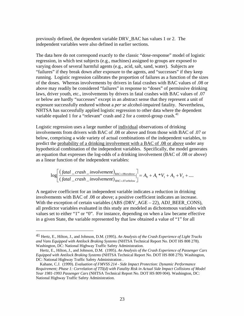
The data here do not correspond exactly to the classic ldquodose-responserdquo model of logistic regression in which test subjects (eg machines) assigned to groups are exposed to varying doses of several harmful agents (eg acid salt sand water) Subjects are ldquofailuresrdquo if they break down after exposure to the agents and ldquosuccessesrdquo if they keep running Logistic regression calibrates the proportion of failures as a function of the sizes of the doses Whereas involvements by drivers in fatal crashes with BAC values of 08 or above may readily be considered ldquofailuresrdquo in response to ldquodosesrdquo of permissive drinking laws driver youth etc involvements by drivers in fatal crashes with BAC values of 07 or below are hardly ldquosuccessesrdquo except in an abstract sense that they represent a unit of exposure successfully endured without a per se alcohol-impaired fatality Nevertheless NHTSA has successfully applied logistic regression to other data where the dependent variable equaled 1 for a ldquorelevantrdquo crash and 2 for a control-group crash41
Logistic regression uses a large number of individual observations of drinking involvements from drivers with BAC of 08 or above and from those with BAC of 07 or below comprising a wide variety of actual combinations of the independent variables to predict the probability of a drinking involvement with a BAC of 08 or above under any hypothetical combination of the independent variables Specifically the model generates an equation that expresses the log-odds of a drinking involvement (BAC of 08 or above) as a linear function of the independent variables
A negative coefficient for an independent variable indicates a reduction in drinking involvements with BAC of 08 or above a positive coefficient indicates an increase With the exception of certain variables (ABS (DRV_AGE ndash 22) ADJ_BEER_CONS) all predictor variables evaluated in this study are modeled as dichotomous variables with values set to either ldquo1rdquo or ldquo0rdquo For instance depending on when a law became effective in a given State the variable represented by that law obtained a value of ldquo1rdquo for all
41 Hertz E Hilton J and Johnson DM (1995) An Analysis of the Crash Experience of Light Trucks and Vans Equipped with Antilock Braking Systems (NHTSA Technical Report No DOT HS 808 278) Washington DC National Highway Traffic Safety Administration
Hertz E Hilton J and Johnson DM (1995) An Analysis of the Crash Experience of Passenger Cars Equipped with Antilock Braking Systems (NHTSA Technical Report No DOT HS 808 279) Washington DC National Highway Traffic Safety Administration
Kahane CJ (1999) Evaluation of FMVSS 214 - Side Impact Protection Dynamic Performance Requirement Phase 1 Correlation of TTI(d) with Fatality Risk in Actual Side Impact Collisions of Model Year 1981-1993 Passenger Cars (NHTSA Technical Report No DOT HS 809 004) Washington DC National Highway Traffic Safety Administration
23
crashes that occurred during the period after the law was in effect and ldquo0rdquo for all crashes that occurred during the period prior to the effective date of the law
24
Results
Now let us assess the effects of alcohol programs plus other factors (ie demographic external and alcohol consumption) that could explain the decline in alcohol-impaired driving trend ndash the actual proportion of drivers in fatal crashes with BAC of 08 or above from 1982-1997 and the leveling off from 1998-2005 (Figure 3) First we will discuss the parameter estimates of the logistic regression model ndash that is based on a set of independent variables previously discussed as possible significant contributors to the historical alcohol-impaired driving trend from 1982 to 2005 Next we will (1) see whether the trend predicted by the regression model (specifically the trend of the expected proportion of drivers in fatal crashes with BAC of 08 or above from 1982 to 2005) reproduces the actual trends of declines in alcohol-impaired driving from 1982 to 1997 leveling out after 1997 (2) determine how much of the overall reduction in alcohol-impaired fatalities involving drivers in fatal crashes with BAC of 08 or higher is due to the introduction of laws and how much is due to demographic factors and reductions in alcohol consumption and (3) estimate the percentage of reduction attributable to specific factors such as individual laws
Table 4 shows the regression coefficients of all the independent variables considered in the analysis The positive coefficient (06677) of the ldquogenderrdquo variable DRVMALE (equals 1 for male 0 for female) indicates that male drivers involved in fatal crashes are more likely to be drinking and have BAC at or above a 08 level than females The negative coefficient (-00264) of the driver age factor variable ABS (DRV_AGE ndash 22) also shown in Table 4 ndash indicates that the probability of drinking (BAC of 08 or above) is highest at age 22 and it decreases for each year that the driver is older or younger than 22 The model also predicts that the likelihood of alcohol involvement in a fatal crash is substantially higher at night than during the day ndash coefficient estimate of 16306 for the variable NITE It is also higher on a rural roadway than on an urban roadway Furthermore the positive coefficient for the adjusted ethanol consumption in beer (ADJ_BEER_CONS) suggests that higher beer consumption will translate to a higher proportion of drivers in fatal crashes with BAC of 08 or higher As explained in Section B of ldquoIndependent Variablesrdquo per capita consumption is known only at the State and calendar year level We know nothing about the drinking habits of the individual drivers involved in the crashes The variable has already been adjusted for the populationrsquos age distribution in the State that year in order not to ldquodouble countrdquo the demographic effects of the aging population
As for other external factors such as WEEKDAY (equals 1 if occurred on a weekday 0 on a weekend) and SPDLIM55 (equals 1 if posted speed limit is 55 or greater 0 otherwise) the model predicts that the probability of an alcohol-impaired fatal crash involvement is lower for a weekday crash than a weekend crash and also lower on a roadway with posted speed limit of 55 or greater ndash as shown in Table 4 by the negative coefficients -05522 and -01295 respectively
25
As for the alcohol laws a negative coefficient indicates that the law is beneficial reducing the proportion of drivers in fatal crashes who had BAC of 08 or above The analysis method of this report is not ideal for precisely quantifying the benefits of specific laws for that purpose more narrowly focused time-series analyses for individual States before and after the specific law might be more suitable Nevertheless the regression shows a statistically significant benefit (as evidenced by the negative coefficients and significant t-values) for each of the variables PT10 MLDA21 ALR PT08 and ZT21
Table 4 Regression Analysis of Demographic Other External Factors Adjusted Alcohol Consumption and Alcohol Laws Variables
Parameter Estimate Standard Error
t for H0 Parameter=Theta0 Pr gt|t|
Intercept -22562 00194 -11652 lt0001 DRVMALE 06677 00075 8866 lt0001
ABS (DRV_AGE-22) -00264 00003 -10537 lt0001 WEEKDAY -05522 00061 -9045 lt0001
NITE 16306 00063 25920 lt0001 SPDLIM55 -01295 00059 -2208 lt0001
RURAL 03102 00060 5202 lt0001 ADJ_BEER_CONS 05179 00147 3526 lt0001
PT10 -01124 00086 -1305 lt0001 MLDA21 -07543 00103 -7329 lt0001
ALR -01027 00067 -1543 lt0001 PT08 -01177 00071 -1648 lt0001 ZT21 -01862 00150 -1242 lt0001
The coefficients shown in Table 4 for the independent variables calibrate a linear relationship between the independent variables and the logarithm of the odds that a driver in a fatal crash was drinking and had BAC of 08 or above We however are less interested in the log odds than in the probability that a driver involved in a fatal crash had a BAC of 08 or above This probability is derived from our regression ndash as shown in the equations below
26
PDRV _ BAC=1 = Z (1 + Z )
where
Z = exp(minus22562 + 06677 DRVMALE minus 00264 ABS(DRV _ AGE minus 22) minus 05522 WEEKDAY +16306 NITE minus 01295 SPDLIM 55 + 03102 RURAL + 05179 ADJ _ BEER _ CONS minus 01124 PT10 minus 07543 MLDA21 minus 01027 ALR minus 01177 PT 08 minus 01862 ZT 21)
For any specific driver in FARS the expected probability that this specific driver had BAC gt= 08 is calculated by entering the values of all the independent variables for that driver into the above equations For example Table 5 shows what values would be entered if the driver is a 27-year-old male in Alaska in 1995 on a rural 55 mph road at noon on Sunday
The expected probability will be a number between 0 and 1 In our example the expected probability is 03571 For any group of drivers in FARS the expected proportion of drivers with BAC of 08 or above is the average of the individual probabilities In particular we are interested in the expected proportion of drivers with BAC of 08 or above among all the drivers of any calendar year These average proportions by calendar year are the trend line predicted by our regression model Using the PROC MEANS procedure of SAS the probability of an alcohol-impaired involvement in a fatal crash by calendar year from 1982 to 2005 can then be calculated and graphed accordingly
Table 5 Values of the Independent Variables Used in the Initial Probability Equation (Example of a 27-year-old male in Alaska in 1995 on a rural 55 mph road at noon on Sunday)
Independent Variables Values DRVMALE 1 because male ABS (DRV_AGE ndash 22) 5 = ABS(27-22) WEEKDAY 0 because Sunday NITE 0 because noon SPDLIM55 1 because speed limit is 55 RURAL 1 because rural ADJ_BEER_CONS 140 (adjusted per capita beer consumption in Alaska in 1995 - see
Appendix C) PT10 1 because 10 BAC had been in effect since 1983 MLDA21 0 because driver is age 21+ ALR 1 because ALR had been in effect since 101983 PT08 0 because 08 BAC did not go into effect until 092001 ZT21 0 because driver is age 21+
27
Figure 8 Proportion of Alcohol-Impaired Involvement of Drivers in Fatal Crashes - BAC of 08 or Above (Expected versus Actual)
0350
0200
0336
0216
0180
0200
0220
0240
0260
0280
0300
0320
0340
0360
0380
Prop
ortio
n of
Alc
ohol
-Im
pair
ed In
volv
emen
t
Actual Proportion of Drivers (BAC 08 or above)
Expected - P(drivers w ith BAC 08 or above)
2005
2004
2003
2002
2001
2000
1999
1998
1997
1996
1995
1994
1993
1992
1991
1990
1989
1988
1987
1986
1985
1984
1983
1982
CY
Figure 8 shows the trend lines of both the expected and the actual proportion of drivers in fatal crashes with BAC of 08 or above from 1982 to 2005 The trends in this figure show that the actual proportion of drivers in fatal crashes with BAC of 08 or above is higher (to some extent) than the expected prior to 1992 and slightly lower (more or less) than the expected after 1992 In general the average rate of change in the trend line of the actual proportion of drivers in fatal crashes with BAC of 08 or above from 1982 to 1997 is slightly steeper [(0350-0200)16= 0009] when compared with the rate of change in the trend line of the expected [(0336-0216)16=0008] proportion of drivers in fatal crashes with a BAC of 08 or above ndash also from the same time period After 1997 the two trend lines level off (more or less) but the expected drinking proportion is more stable than the actual Overall our model does a good job tracking the actual even though some of the peaks and outliers are smoothed out Hence we can feel quite comfortable using expected effects based on regression formulas to compute the relative contributions of the individual factors
To determine how much of the overall reduction in the proportion of drivers in fatal crashes with BAC of 08 or above is due to demographic external factors and alcohol consumption the values of the alcohol-law variables in the above probability equation are replaced by a new set of values corresponding to the alcohol laws that were in effect on December 31 1981 Table 6 continues our example of the 27-year-old male in Alaska in
28
1995 but now in a hypothetical scenario that alcohol laws were still the same as in 1981 Prior to 1982 none of the studied alcohol laws had been enacted in Alaska Hence for this scenario the values of the individual alcohol-law variables (prior to 1982) are equaled to 0 In our example the expected probability of an alcohol-related involvement of a driver with BAC of 08 or above is 04428 this is higher than the 03571 calculated in Table 5 and demonstrates how risk has increased without PT10 and ALR
Table 6 Values of the Independent Variables Used in the Probability Equation (Controls for Demographic Environment-related Factors and Alcohol Consumption But Not the Laws)
(Example of a 27-year-old male in Alaska in 1995 on a rural 55 mph road at noon on Sunday)
Independent Variables Values DRVMALE 1 ABS (DRV_AGE ndash 22) 5 WEEKDAY 0 NITE 0 SPDLIM55 1 RURAL 1 ADJ_BEER_CONS 140 PT10 0 because not in effect in Alaska on 12311981 MLDA21 0 because driver is age 21+ ALR 0 because not in effect in Alaska on 12311981 PT08 0 because not in effect in Alaska on 12311981 ZT21 0 because driver is age 21+
Similarly if only the demographic and external factors are considered then not only are the values of the alcohol-law variables replaced but also the actual yearrsquos adjusted per capita ethanol consumption in beer is replaced by the adjusted per capita consumption for Alaska in 1982 ndash Table 7 In our example the expected probability of positive BAC (specifically BAC of 08 or above) has further increased to 04736 because per capita beer consumption was higher in 1982 than in 1995
29
Table 7 Values of the Independent Variables Used in the Probability Equation (Controls for Demographic and Environment-related Factors only)
(Example of a 27-year-old male in Alaska in 1995 on a rural 55 mph road at noon on Sunday)
Independent Variables Values DRVMALE 1 ABS (DRV_AGE ndash 22) 5 WEEKDAY 0 NITE 0 SPDLIM55 1 RURAL 1 ADJ_BEER_CONS 153 (adjusted per capita beer consumption in AK in 1982) PT10 0 MLDA21 0 ALR 0 PT08 0 ZT21 0
Figure 9 shows the trend lines of the expected proportion of drivers in fatal crashes with BAC of 08 or above from 1982 to 2005 ndash after controlling for (1) only the demographic and external factors (2) just the demographic and external factors plus alcohol consumption and (3) all factors that are considered in the analysis including the alcohol laws The horizontal line in Figure 9 shows the drinking proportion if (1) the alcohol laws remained unchanged from December 31 1981 (2) per-capita consumption remained at 1982 levels and (3) the age and gender distribution of the driving population remained at the 1982 level ndash that is nothing had changed since 1982 The three trend lines in Figure 9 generally show that the expected proportion of drivers in fatal crashes with BAC of 08 or greater reduced substantially from 1982 to 1998 and leveled off after that Also as illustrated in the figure the demographic factors and the alcohol laws each made a sizeable and growing contribution to the overall reduction in alcohol-impaired involvement among drivers in fatal crashes in 1982-1997 but with little or no further growth from 1998 onwards This will be discussed in depth in the next several sections
30
Figure 9 Expected Proportion of Drinking Involvement Among Drivers With BAC of 08 or Greater in Fatal Crashes
0349
0274
0269
0214
0150
0200
0250
0300
0350
0400
1982
1983
1984
1985
1986
1987
1988
1989
1990
1991
1992
1993
1994
1995
1996
1997
1998
1999
2000
2001
2002
2003
2004
2005
CY
Expe
cted
Pro
port
ion
of A
lcoh
ol-Im
paire
d D
river
s in
Fat
al C
rash
es
Expected - P(BAC 08 or above) wo factors
Expected - P(BAC 08 or above) w demographic environment-related factors Expected - P(BAC 08 or above) w demographic environment-related factors amp consumption Expected - P(BAC 08 or above) w all factors
As previously mentioned in a logistic regression the logarithm of the odds that the dependent variable equals 1 is linearly related to the independent variables Hence quantifying the relative effects of individual factors should be based on the log odds ratio so that (1) the effects are additive and commutative and (2) the results are the same regardless of the order the factors are applied to the regression model The three trend lines in Figure 10 show that the expected log-odds of alcohol-impaired involvement among drivers in fatal crashes reduced substantially from 1982 to 1998 and leveled off after that As shown by the cross-shaped curve the expected log-odds of BAC of 08 or above for drivers involved in fatal crashes dropped from -0623 to -1301 by 1998 ndash an overall reduction of 0678 in the log-odds The log-odds dropped a little more in 1998-2005
31
Figure 10 Expected Log Odds of Alcohol-Impaired Involvement of Drivers in FatalCrashes with BAC of 08 or Above
-0623
-0974
-1000
-1301
-1470
-1370
-1270
-1170
-1070
-0970
-0870
-0770
-0670
-0570
Log
Odd
s of D
rink
ing
Invo
lvem
ent
Expected Log Odds (BAC gt= 08) wo factors
Expected Log Odds (BAC gt= 08) w demographic environment-related factors
Expected Log Odds (BAC gt= 08) w demographic environment-related factors amp consumption
Expected Log Odds (BAC gt= 08) w all factors
2005
2004
2003
2002
2001
2000
1999
1998
1997
1996
1995
1994
1993
1992
1991
1990
1989
1988
1987
1986
1985
1984
1983
1982
CY
Now let us find out how much of that reduction is explained by driver age and gender specifically how much of the reduction is due to the fact that the driving population became older and proportionately more female ndash and therefore less likely to have been drinking and by other external factors (particularly day of the week time of day roadway function class and posted speed limit) When we assumed that alcohol laws and per capita alcohol consumption remained the same as in 1982 and modeled only the demographic change the expected log-odds of drivers in fatal crashes with BAC of 08 or above reduced from -0623 to -0974 in 1998 the year with the lowest (more or less) percentage of alcohol-impaired involvement among drivers in fatal crashes a reduction of 0351 as shown in the square-shaped curve In other words the aging of the population and the greater proportion of female drivers along with other external factors explained more than one-half [(0351) (0678) = 052] of the overall decrease in the log-odds of alcohol-impaired involvements among drivers in fatal crashes by 1998 This part of the reduction is due simply to demographic changes and would have presumably occurred even without any programs to discourage drinking and driving After 1998 the log-odds increased a little as illustrated in Figure 10 by the slight upward trend
The alcohol consumption variable is conceptually somewhere between the purely ldquoexternalrdquo demographic variables and the State laws that are directly under the
32
governmentrsquos control Even though per capita alcohol consumption is certainly not under the direct control of governments their policies conceivably have a limited effect on per capita consumption to the extent that they influence public attitudes regarding alcohol ndash it is the aggregate effect of individualsrsquo choices about whether to drink how often and how much When the change in per capita beer consumption is taken into consideration in addition to the demographic effect the log-odds of an alcohol-impaired involvement by 1998 decreased from -0974 on the square shaped curve to -1000 (as shown on the triangle-shaped curve in Figure 10) ndash a reduction of 0026 Hence only 4 percent (0026 0678) of the overall reduction is attributed to lower alcohol consumption (specifically beer consumption)
As for the five alcohol laws considered in this analysis Figure 10 shows the expected log-odds of an alcohol-related involvement among drivers in fatal crashes was reduced by 1998 from -1000 on the triangle shaped curve to -1301 on the cross-shaped curve (a reduction of 0301) ndash when the alcohol laws are included in the analysis along with the demographic factors and alcohol consumption The laws account for 44 percent (0301 0678) of the overall log-odds reduction As previously pointed out the log-odds reduced a little more in 1998-2005
As shown previously in Figure 7 the number of alcohol laws that were passed in all States steadily increased from 36 in 1982 to 204 in 1997 and the pace of their introduction gradually slowed down after that The increase from 36 laws in 1982 to 204 in 1997 is a long-term rate of 112 new laws per year actually gaining to 135 new laws per year from 1993 to 1997 whereas the subsequent increase from 204 laws in 1997 to 245 laws in 2005 is 51 new laws per year Hence many of these laws were already in effect by 1997 Indeed Figure 11 shows that all of these laws except the 08 BAC were in place entirely or largely by 1997 Three-fourths of the States did not pass the 08 BAC laws until after 1997 Because the majority of their impact is felt in the earlier years that might explain the substantial reduction in the proportion of alcohol-related involvements among drivers in fatal crashes with BAC of 08 or higher from 1982 to 1998 and the small additional reduction from 1998 to 2005 (specifically after 2002) The aging of the population (specifically the majority of the baby-boomer generation turned 35 by 1998 and left their drinking years behind) and the increased proportion of female drivers (ie female drivers accounted for nearly half of the driving population by 1997 and leveled off after that) may further explain the level trend from 1998 to 2005 In fact the trends from these factors (ie demographic and alcohol laws) well depict the national historical alcohol-impaired driving trend before and after 1998
33
Figure 11 Number of States That Enacted Acohol Laws (by Year and by Law)
0
10
20
30
40
50
60
1982
1983
1984
1985
1986
1987
1988
1989
1990
1991
1992
1993
1994
1995
1996
1997
1998
1999
2000
2001
2002
2003
2004
2005
CY
Tot
al
Sta
tes
PT10 MLDA-21 PT08 ZT21 ALR
Effects of Individual Laws
As previously discussed the analysis method of this report is not ideal for precisely quantifying the benefits of specific laws for that purpose more narrowly focused time-series analyses for individual States before and after the specific law might be more suitable Nevertheless the regression shows statistically significant benefits for each of the laws Therefore it is worthwhile to analyze these laws more in depth by computing the effectiveness of each of the laws based on the ldquoexpectedrdquo drinking proportion by drivers involved in fatal crashes (BAC of 08 or above) with and without the law ndash by comparing two hypothetical scenarios one of which assumes that all States enacted the law and the other assumes that none of the States enacted the law These expected probabilities are computed by the regression equation for two sets of values for the independent variables The first set of values corresponding to the first scenario sets the variable for the law in question to 1 on all cases The second scenario always sets it to 0 All the other independent variables are set identically in the two scenarios to their original values For example Table 8 shows the values of the independent variables used in the probability equation to analyze the effectiveness of the ALR law
34
Effectiveness = 1minus P(BAC gt= 08) law divide
P(BAC =lt 07) law P(BAC gt= 08)no _ law P(BAC =lt 07)no _ law
Table 8 Values of the Independent Variables Used in the Probability Equation To Analyze the Effectiveness of ALR Law
Independent Variables Without ALR law With ALR law DRVMALE Original FARS-derived value Original FARS-derived value ABS (DRV_AGE ndash 22) Original FARS-derived value Original FARS-derived value WEEKDAY Original FARS-derived value Original FARS-derived value NITE Original FARS-derived value Original FARS-derived value SPDLIM55 Original FARS-derived value Original FARS-derived value RURAL Original FARS-derived value Original FARS-derived value ADJ_BEER_CONS Original value from Appendix D Original value from Appendix D PT10 Original value from Table 1 Original value from Table 1 MLDA21 Original value from Table 1 Original value from Table 1 ALR 0 1 PT08 Original value from Table 1 Original value from Table 1 ZT21 Original value from Table 1 Original value from Table 1
The averages of the individual expected probabilities with and without the law are then calculated for a full year of FARS data The overall effectiveness of the law is computed from these two averages by treating the crash involvements among drivers who had BAC of 07 or less as a control group
where P is the expected probability of drivers in fatal crashes The overall effectiveness is the absolute percentage reduction in fatal crash involvements of drivers with BAC of 08 or above
As shown in Figure 11 the MLDA-21 and 10 BAC per se laws were already in effect in the majority of States by 1988 whereas the other laws were not enacted in most States until later Hence crash data from calendar year 1988 were used for the effectiveness analysis of the MLDA-21 and 10 BAC laws The reason for using 1988 as the baseline year when estimating the effects of these two laws is because the majority of States (if not all) had already passed these laws by 1988 but at the same time only a handful of States had adopted the Zero Tolerance and 08 BAC laws It does not make much sense to evaluate these two laws in an environment (ie crash data from mid-1990s or 2000s) where most States already have the Zero Tolerance and 08 laws We could have chosen another calendar year as long as the chosen year is before the years when States began to adopt the Zero Tolerance and 08 BAC laws and the effectiveness estimates for the two laws (MLDA-21 and 10 BAC) would have been similar to those found in 1988
Theoretically if a 08 law is in effect then a 10 BAC law is implicitly also in effect Similarly every State had already enacted MLDA-21 by the time they enacted Zero
35
Table 9 The Effects of Individual Laws on Drivers With BAC of 08 or Above
Laws Expected Probability of Drivers in Fatal Crashes
Reduction of Fatal Crash Involvements by Drivers with
BAC of 08 or Above
Base Year BAC of 08 or Above
BAC of 07 or below
()
ALR Law 02047 07953 No ALR Law
2005 02189 07811
8
PT10 02681 07319 No PT10 Law 1988 02867 07133 9
PT08 02065 07935 No PT08 Law 2005 02233 07767 9
MLDA21 02403 07597 No MLDA21 1988 03747 06253 47
ZT21 01653 08347 No ZT21 Law
2005 01893 08107
15
Analysis limited to drivers younger than 21
Tolerance Thus in these two analyses the 10 BAC law is always 1 when the 08 BAC law is set to 1 and the MLDA-21 law is always 1 when the Zero Tolerance law equals 1 For the effectiveness analysis of the Zero Tolerance 08 BAC per se and ALR calendar year 2005 was used as the baseline year because it is the latest year available and by 2005 all States had enacted the 08 BAC and Zero Tolerance laws and 42 States had passed the ALR laws
Table 9 shows that the laws are beneficial in reducing the proportion of drivers in fatal crashes with BAC of 08 or above ndash as indicated by the positive effectiveness estimates (highlighted in bold) It is estimated that the ALR laws had an 8-percent reduction of fatal crash involvements by drivers with BAC of 08 or above The introduction of the 10 BAC laws had a similar impact ndash as shown by the 9-percent reduction We also found that the 08 BAC laws had a 9 percent-reduction in the proportion of drivers (BAC of 08 or above) in fatal crashes The reductions for these three laws apply to drivers of all ages As previously discussed since both MLDA-21 and Zero Tolerance laws were mandated to target youths and to prevent them from drinking and driving until they reach the age of 21 only FARS cases where drivers who are less than 21 years of age are included in the analyses of the two laws ndash because the laws added no benefits to those ages 21 and older The effects that these two laws (MLDA-21 and Zero Tolerance) had on drivers ages 20 and under are strong ndash as demonstrated in Table 9 by the 47 percent and 15 percent reductions of fatal involvements by drivers with BAC of 08 or above The results found in this study are also comparable to those found in studies previously mentioned in the ldquoBackground information on alcohol lawsrdquo Section
36
Analysis of Alcohol-Related Driving Trends Involving Drivers With BAC of 01 or Above
As previously mentioned in the ldquoMotivation for This Studyrdquo Section the alcohol-related driving trend (where drivers involved in fatal crashes had BAC of 01 or above) is similar to the alcohol-impaired driving trend where crash-involved drivers had BAC of 08 or above We have discussed in detail how the effects of alcohol laws demographic trends and lower alcohol consumption influenced the impaired driving trend (specifically the proportion of drivers involved in fatal crashes with BAC of 08 or above from 1982 to 2005) It is also worthwhile to analyze similar programs to determine if they have the same effects on drivers involved in fatal crashes with BAC of 01 or above In other words we are interested in the general deterrent effects (if any) of these programs on drivers involved in fatal crashes who had been drinking but were not necessarily alcohol-impaired at the time of the crash
In the latter analysis we also modeled the effect on a binary dependent variable but the variable has a value of 1 for drivers with BAC of 01 or above and a value of 2 for all other drivers The regression coefficients of all the independent variables considered in the latter analysis (shown in Table 10) also indicate that male drivers involved in fatal crashes are more likely to be drinking (BAC of 01 or above) than females Similar to the previous analysis result the probability of drinking is highest at age 22 and it decreases for each year that the driver is older or younger than 22 ndash as shown by the negative coefficient Furthermore the likelihood of an alcohol-related involvement in a fatal crash is higher (1) at night than during the day and (2) on a rural roadway than on an urban roadway The results also suggest that higher beer consumption will translate not only to higher proportion of drivers with BAC of 08 or above but also to higher proportion of drivers with BAC of 01 or above The model predicts that the probability of a fatal crash involvement by a driver who had BAC of 01 or above is also lower for a weekday crash than a weekend crash and lower on a roadway with posted speed limit of 55 or greater Furthermore the laws are also beneficial in reducing the proportion of drivers in fatal crashes with BAC of 01 or above ndash though the method of quantifying the benefits of these laws (as previously discussed) may not be appropriate
37
Table 10 Regression Analysis of Demographic Other External Factors Adjusted Alcohol Consumption and Alcohol Laws Variables ndash BAC of 01 or Above
Parameter Estimate Standard Error
t for H0 Parameter=Theta0 Pr gt|t|
Intercept -19582 00187 -10490 lt0001 DRVMALE 06860 00073 9454 lt0001
ABS (DRV_AGE-22) -00276 00002 -12988 lt0001 WEEKDAY -05941 00051 -11545 lt0001
NITE 16359 00058 28420 lt0001 SPDLIM55 -01401 00057 -2463 lt0001
RURAL 03083 00054 5760 lt0001 ADJ_BEER_CONS 05333 00139 3844 lt0001
PT10 -01224 00081 -1517 lt0001 MLDA21 -06287 00089 -7047 lt0001
ALR -01119 00060 -1850 lt0001 PT08 -01147 00068 -1683 lt0001 ZT21 -02241 00135 -1657 lt0001
Similar to Figure 10 Figure 12 shows the trend lines of the expected log-odds of an alcohol-related involvement of drivers in fatal crashes with BAC of 01 or above after controlling for (1) demographic and external factors (square-shaped curve) (2) demographic factors and alcohol consumption (triangle-shaped curve) and (3) all factors including the alcohol laws (cross-shaped curve) Using the same calculation method previously discussed demographic changes explained 53 percent of the overall reduction in the proportion of drivers involved in fatal crashes with BAC of 01 or above lower alcohol consumption accounted for 3 percent and the remaining 44 percent is attributed to the alcohol laws
Table 11 shows the effects of individual laws based on the average of the individual expected probabilities of drivers in fatal crashes with BAC of 01 or above controlling for those with BAC of 00 As expected the laws are just as beneficial in reducing the proportion of drivers in fatal crashes with BAC of 01 or above as they are with drivers who had BAC of 08 or higher
38
Figure 12 Expected Log Odds of Alcohol-Related Involvement of Drivers in Fatal Crashes With BAC of 01 or Above
-0393
-0754
-0777
-1077
-1170
-1070
-0970
-0870
-0770
-0670
-0570
-0470
-0370
1982
1983
1984
1985
1986
1987
1988
1989
1990
1991
1992
1993
1994
1995
1996
1997
1998
1999
2000
2001
2002
2003
2004
2005
CY
Log
Odd
s of D
rink
ing
Invo
lvem
ent
Expected Log Odds (BAC of 01 or above) wo factors
Expected Log Odds (BAC of 01 or above) w demographic environment-related factors
Expected Log Odds (BAC of 01 or above) w demographic environment-related factors amp consumption Expected Log Odds (BAC of 01 or above) w all factors
Laws
Table 11 The Effects of Individual Laws on Drivers With BAC of 01 or Above
Expected Probability of Drivers in Fatal Crashes
Reduction of Fatal Crash Involvements by Drivers
with BAC of 01 or Above
Base Year BAC of 01 or Above BAC = 0 () ALR Law 2005 02446 07554 9 No ALR Law 02617 07383
PT10 No PT10 Law 1988 03177
03394 06823 06606 9
PT08 No PT08 Law 2005 02468
02649 07532 07351 9
MLDA21 No MLDA21 1988 03115
04317 06885 05683 40
ZT21 No ZT21 Law
2005
Analysis limited to drivers younger than 21
02161 02505
07839 07495
18
39
Conclusions
In summary the change in the alcohol-related driving trends (1) the proportion of drivers in fatal crashes who had BAC of 08 or above and (2) the proportion of drivers with BAC of 01 or above in fatal crashes decreasing from 1982 to 1997 and leveling off after 1997 can largely be explained by the following
bull Alcohol laws (44 of the change) minus The minimum legal drinking age (MLDA-21 Zero Tolerance) 10 BAC
08 BAC and ALR laws were very effective in deterring alcohol-related fatal crashes involving drivers who had been drinking at the time of the crash
minus Most of the laws were already in effect in most of the States by 1997 Hence the majority of the improvements in alcohol-related fatal crash involvements (due to the laws) occurred before 1997 The 08 BAC law is the only law that was passed in a large number of States since 1997 As a result small additional improvements in alcohol-related crashes occurred after 1997
minus The leveling off by and large after 1997 does not imply that the laws are becoming less effective On the contrary they effectively maintain the proportion of drivers involved in fatal crashes who had been drinking
bull Demographic trends (52 of the change) minus As the driving population became older (specifically the majority of the
baby-boomer generation turned 35 by 1998) they tended to drink less and thus were less likely to be involved in alcohol-related fatal crashes
minus The increasing numbers and annual mileage of female drivers Female drivers accounted for nearly half of the driving population by 1997 and that proportion did not change after that) females are less likely to drink and drive than males
minus The leveling off of these demographic trends circa 1998 (and even a slight reversal in the trend toward an aging driver population in the last few years) further explains much of the leveling off in the proportion of drivers involved in fatal crashes at all BAC levels42
bull Lower per capita alcohol consumption (4 of the change) minus Although the model predicts a statistically significant reduction in the
proportion of drivers in fatal crashes who had been drinking at all BAC levels the fatality reduction part attributed by the analysis to this factor is substantially less than the effects of the laws and demographic trends
42 The slight reversal in the aging driver population trend in recent years may explain why the actual proportion of drivers who had been drinking at the time of the crash levels off after 1997 even though there are small additional improvements (due to the 08 BAC per se laws) in alcohol-related crashes after 1997
40
minus The decrease in per capita alcohol consumption had leveled off by 1997
In summary demographics and alcohol laws each explain similar proportions of the overall reduction in alcohol-related fatal crash involvements among drivers with BAC of 08 or above and among those with BAC of 01 or higher The laws provide similar benefits to those drivers as well
41
REFERENCES
NHTSA (2001) Alcohol Involvement in Fatal Crashes 1998 (NHTSA Technical Report No DOT HS 809 103) Washington DC National Highway Traffic Safety Administration
NHTSA (2005) Alcohol Involvement in Fatal Motor Vehicle Traffic Crashes 2003 (NHTSA Technical Report No DOT HS 809 822) Washington DC National Highway Traffic Safety Administration
Apparent Per Capita Ethanol Consumption for the United States 1850-2004 accessible from wwwniaaanihgovdatabasesqfhtmcons
Cucchiaro S Ferreira J and Sicherman A (1974) The Effect of the 18-Year-Old Drinking Age on Auto Accidents Cambridge MA Massachusetts Institute of Technology Operations Research Center
Current Population Reports ndash Resident Population by Age and State 1982-2005 Washington DC United States Census Bureau
Dennis ME (1995) Effects of Alcohol on Driving Task Abilities American Drivers and Traffic Safety Education Association ndash The Chronology Indiana PA Summer Issue
Douglass RL Filkins LD and Clark FA (1974) The Effect of Legal Drinking Ages on Youth Crash Involvement Ann Harbor MI University of Michigan Highway Safety Research Institute
Effectiveness of 008 Percent Blood Alcohol Concentration (BAC) Laws CDC Community Guide 2001
Hertz E Hilton J and Johnson D (1995) An Analysis of the Crash Experience of Passenger Cars Equipped with Antilock Braking Systems (NHTSA Technical Report No DOT HS 808 279) Washington DC National Highway Traffic Safety Administration
Hertz E Hilton J and Johnson D (1995) An Analysis of the Crash Experience of Light Trucks and Vans Equipped with Antilock Braking Systems (NHTSA Technical Report No DOT HS 808 278) Washington DC National Highway Traffic Safety Administration
Hingson RW et al (1994) Lower Legal Blood Alcohol Limits for YoungDrivers Public Health Reports
Hingson RW Assailly JP and Williams AF (2004) Underage Drinking Frequency Consequences and Intervention Traffic Injury Prevention 5(3) 228-236
42
Hingson R Heeren T and Winter M (1996) Lowering State Legal Blood Alcohol Limits to 008 Percent The Effect on Fatal Motor Vehicle Crashes American Journal of Public Health 86(9) 1297-1299
History of SADD accessible from wwwsaddonlinecomhistoryhtm
Jones J (2006) US Drinkers Consuming Alcohol More Regularly ndash Beer Regains Slight Edge Over Wine as Preferred Drink Washington DC The Gallup Poll News Service
Jones RK and Lacey JH (2001) Alcohol and Highway Safety 2001 A Review of the State of Knowledge (NHTSA Technical Report No DOT HS 809 383) Washington DC National Highway Traffic Safety Administration
Kahane CJ (1999) An Evaluation of FMVSS 214 ndash Side Impact Protection Dynamic Performance Requirement Phase 1 Correlation of TTI(d) with Fatality Risk in Actual Side Impact Collisions of Model Year 1981-1993 Passenger Cars (NHTSA Technical Report No DOT 809 004) Washington DC National Highway Traffic Safety Administration
Klein T (1986) A Method for Estimating Posterior BAC Distributions for Persons Involved in Fatal Traffic Accidents (NHTSA Technical Report No DOT HS 807 094) Washington DC National Highway Traffic Safety Administration
Klein TM (1989) Change in Alcohol-Involved Fatal Crashes Associated with Tougher State Alcohol Legislation (NHTSA Technical Report No DOT HS 807 511) Washington DC Sigmastat Inc
MADD Milestones accessible from wwwmaddorgaboutus11056117900html
Per Capita Ethanol Consumption for States Census Regions and the United States 1970-2003 accessible from wwwniaaanihgovdatabasesqfhtmcons
Percent Reporting Heavy Alcohol Use in the Past Month by Age Group and Demographic Characteristics NHSDA 1994-97 accessible from wwwniaaanihgovdatabasesqfhtmdkpat
Research and Evaluation Associates (1991) The Effects Following the Implementation of an 008 BAC Limit and an Administrative Per Se Law in California (NHTSA Technical Report No DOT HS 807 777) Washington DC National Highway Traffic Safety Administration
43
Rubin D (1987) Multiple Imputation of Nonresponse in Surveys JWiley and Sons New York
Subramanian R (2002) Transitioning to Multiple Imputation ndash A New Method to Impute Missing Blood Alcohol Concentration (BAC) Values in FARS (NHTSA Technical Report No DOT HS 809 403) Washington DC National Highway Traffic Safety Administration Stewart K (2000) On DWI Laws in Other Countries (NHTSA Report No DOT HS 809 037) Washington DC National Highway Traffic Safety Administration
The Effects Following the Implementation of a 008 BAC Limit and an Administrative Per Se Law in California (NHTSA Technical Report No DOT HS 807 777) Washington DC National Highway Traffic Safety Administration 1991
The Minimum Legal Drinking Age Facts and Fallacies accessible from wwwama-assnorgamapubarticle3566-3640html
Traffic Safety Facts 2002 (NHTSA Technical Report No DOT HS 810 620) (2003) Washington DC National Highway Traffic Safety Administration
Traffic Safety Facts 2005 (Early Edition) (NHTSA Technical Report No DOT HS 810 631) (2006) Washington DC National Highway Traffic Safety Administration
Traffic Safety Facts 2005 (Early Edition) (NHTSA Technical Report No DOT HS 810 631) (2006) Washington DC National Highway Traffic Safety Administration
Voas RB and Tippetts AS (1999) The Relationship of Alcohol Safety Laws to Drinking Drivers in Fatal Crashes (NHTSA Technical Report No DOT HS 808 890) Washington DC National Highway Traffic Safety Administration
Voas RB Tippetts AS and Taylor EP (1999) Impact of Ohio Administrative License Suspension Journal of Crash Prevention and Injury Control
Wagenaar AC Zobek TS Williams GD et al (2000) The Effects of DWI Control Efforts a Systematic Review of the Literature from 1960-1991 Minneapolis MN University of Minnesota School of Public Health
Williams AF Rich RF Zador PL and Robertson LS (1974) The Legal Minimum Drinking Age and Fatal Motor Vehicle Crashes Washington DC Insurance Institute for Highway Safety
Zador PL Lund AK Fields M and Wienberg K (1988) Fatal Crash Involvement and Laws Against Alcohol-Impaired Driving Washington DC Insurance Institute for Highway Safety
44
Appendix A
45
Figure A1 Actual Proportion of Drivers With BAC = 01 or Above in Fatal Crashes 1982-2005
0200
0250
0300
0350
0400
0450
Actual Proportion of Drivers (BAC of 01 or Above)
2005
2004
2003
2002
2001
2000
1999
1998
1997
1996
1995
1994
1993
1992
1991
1990
1989
1988
1987
1986
1985
1984
1983
1982
CY
Prop
ortio
n of
Dri
vers
in F
atal
Cra
she
46
Figure A2 US Population Trends by Age (1982-2005)
1000
2000
3000
4000
5000
6000
7000
8000
Under 5 Ages 5-17
Ages 18-24 Ages 25-34
Ages 35-44 Ages 45-64
Ages 65 and over
2005
2004
2003
2002
2001
2000
1999
1998
1997
1996
1995
1994
1993
1992
1991
1990
1989
1988
1987
1986
1985
1984
1983
1982
CY
Popu
latio
n (in
10
000)
)
46
Appendix B
Figure B1 shows the log odds of drivers43 involved in fatal crashes in all 50 States and the District of Columbia by age and gender ndash lsquoMrsquo for males and lsquoFrsquo for females As illustrated in the figure men involved in fatal crashes are generally more likely to have been drinking than women For men the drinking proportion increases from age 14 to age 21 and decreases steadily from age 21 onward For women the drinking proportion increases from age 14 to age 23 and decreases after age 23 The drinking proportion is at its peak at age 21 for males and 23 for females
A single independent variable ABS (DRV_AGE ndash 22) is used to portray the effect of ldquodriver agerdquo
where
1) DRV_AGE is the actual age of the driver 2) Twenty-two is the average of the peak drinking ages for males (21) and females
(23) 3) ABS is the absolute value In other words ABS (AGE-22) is zero at age 22 and
positive on either side of 22
Figure B2 shows this independent variable as a function of driver age We can then predict from our regression analysis the probability of a drinking involvement (relative to non-drinking) by drivers in fatal crashes for each year of age above and below 22
43 log (drinkersnon-drinkers)
47
Figure B1 Log Average Drinking Drivers in Fatal Crashes by Age and Gender 1982‐2002
Log (Avg Drinking Drivers in Fatal Crashes) M Males F Femalessbquo sbquo
‐ 05 ˆsbquosbquo
‐ 10 ˆ M MM M M MM M M MMsbquo M M M MM M M MMsbquo M M M MM M
‐ 15 ˆ M F F F F FF M MM M Msbquo M F F F F F F F FF F FF MM M M Msbquo F F F FF M M M MM
‐ 20 ˆM F F F F F M M MM M Msbquo M F F F F MM M Msbquo FF F F MM
‐ 25 ˆF F FF F F FF M M Msbquo M M Msbquo F F F
‐ 30 ˆ F F F MM Msbquo F F Msbquo FF F
‐ 35 ˆ FF F Fsbquo F F F Fsbquo F F
‐ 40 ˆ F Fsbquosbquo
‐ 45 ˆsbquosbquo
‐ 50 ˆsbquoŠƒƒˆƒƒƒƒƒƒˆƒƒƒƒƒƒˆƒƒƒƒƒƒˆƒƒƒƒƒƒˆƒƒƒƒƒƒˆƒƒƒƒƒƒˆƒƒƒƒƒƒˆƒƒƒƒƒƒˆƒƒƒƒƒƒˆƒƒƒƒƒƒˆƒƒƒƒƒƒˆƒƒƒƒƒƒˆƒƒƒƒƒƒˆƒƒƒƒƒƒˆƒƒƒƒƒƒˆƒƒƒƒƒƒˆƒƒ
16 20 24 28 32 36 40 44 48 52 56 60 64 68 72 76 80
Age
48
Figure B2 ABS (DRV_AGE - 22) As a Function of Driver Age
0
10
20
30
40
50
60
70
80
ABS (DRV_AGE - 22)
95928986838077747168656259565350474441383532292623201714
Driver Age
AB
S (D
RV
_AG
E -
22)
49
Appendix C
This section will discuss step-by-step how to calculate the adjusted per capita ethanol consumption (specifically for beer) by State and by year using available population alcohol consumption and self-reported drinking data The adjusted per capita ethanol consumption for beer expressed as ADJ_BEER_CONS in the analysis is a continuous variable To calculate for the values of this variable both the US and State population by year (1982-2005) and by age group (Under 5 5-17 18-24 25-34 35-44 45-64 65 and up) are obtained from the US Bureau of the Census44 As discussed in the previous section the US and State per capita ethanol consumption by year are available for the entire population and not for the individual age groups However consumption data by age group can be estimated by using the available population data (by age group) and ldquopercent self-reporting heavy alcohol use in the past monthrdquo survey data (also by age group) from the National Household Survey on Drug Abuse45 A person who has had at least 5 drinks per occasion on 5 or more days in the past 30 days is considered to be a heavy alcohol user Since the self-reported drinking data was only available from 1994 to 2002 the average percent is used and the data had to be extrapolated to estimate the average percent of heavy alcohol users for each of the above-mentioned seven age groups and are shown below
Age Group Percentage of Population Who Were Heavy Alcohol
Users (1994-2002 Average)
Under age 5 00 Ages 5-17 27
Ages 18-24 128 Ages 25-34 76 Ages 35-44 57 Ages 45-64 38 Over age 64 22
Entire Population 49
For example for the age group 18-24 128 percent of this age group population reported that they had 5 or more drinks per occasion on 5 or more days in the past 30 days
The following sections continue to discuss step-by-step calculations and provide examples for each of them First the proportion of the population by age group is calculated by dividing the population of each age group by the total population Total population is the sum of the population of all the age groups (Example 1)
44 Current Population Reports ndash Resident Population By Age and State 1982-2005 Washington DC United States Census Bureau 45 Percent Reporting Heavy Alcohol Use in the Past Month by Age Group and Demographic Characteristics NHSDA 1994-1997 accessible from wwwniaaanihgovdatabasesqfhtmdkpat
50
Example 1 State = Alaska Year = 1995
Under 5 5-17 18-24 25-34 35-44 45-64 65 amp up Total AK Population
(000) 53 136 62 91 116 115 30 603
Proportion of AK total population 00879 02255 01028 01509 01924 01907 00498 10000
The percentage of the population (for each age group) is multiplied by the estimated 1994-2002 US average percentage of alcohol users for that age group If Alaska in 1995 had the same rates of heavy drinking in each age group as the national average for 1994-2002 the percent of the total population expected to be heavy users based on their age is the sum of the proportion of users of all the age groups ndash in bold and highlighted in gray in Example 2
Example 2 State = Alaska Year = 1995
Under 5 5-17 18-24 25-34 35-44 45-64 65 amp up Total Proportion of AK total population 00879 02255 01028 01509 01924 01907 00498 10000
Avg proportion of heavy users 0 0027 0128 0076 0057 0038 0022 Proportion of AK population
expected to be heavy users based on their age 0 00061 00132 00115 00110 00072 00011 00501
In other words because the population of Alaska in 1995 is younger than the population of the United States in 1994-2002 we would expect a slightly higher percentage of heavy drinkers 501 rather than 485 even if Alaskans had the same per capita consumption as other Americans of the same age The ratio of these two percentages is used to age-adjust the per capita consumption ndash Example 3
Example 3
Given State = Alaska Year = 1995 Alaska unadjusted per capita consumption (gallons of ethanol in beer) in 1995 = 145
Result Alaska 1995 expected proportion of heavy drinkers 00501 US 1994-2002 actual proportion of heavy drinkers 00485 Alaska adjusted per capita consumption in 1995 145 (0048500501) = 140
In other words if Alaskans in 1995 had the same age distribution as the United States in 1994-2002 their per capita alcohol consumption would have been only 140 not 145 The alcohol consumption was as high as 145 because many Alaskans were young (in their prime drinking years)
51
Appendix D
Numeric variables were used and separately defined to represent the months and the years for each of the laws (Table C-1) Since most of the States passed the 10 BAC and Minimum Legal Drinking Age 21 (MLDA-21) laws during the 1980s and since information on the exact months the laws took effect were no longer readily available the months had to be estimated based on information obtained from the old annual NHTSA legislation compendia and from other sources Thus the dates used for the two laws are estimates of which quarter within the passage year the laws took effect (only the months are estimated the years are not) The decimals 00 25 50 and 75 represent the 1st 2nd 3rd and 4th quarter of a year For example in Table 1 the date when 10 BAC law took effect in Alaska is 8300 which means that its effective date is estimated to be in JanuaryFebruaryMarch of 1983 The 08 BAC ALR and Zero Tolerance 21 laws on the other hand were passed in the last decade or so and information such as implementation dates including specific months was available Thus the dates used for these three laws include the exact months and years
To simplify the analysis the effective dates of all the laws will be converted to decimal numbers with units in years The estimated dates for 10 BAC and MLDA-21 laws are already in decimal numbers with units in years The dates for the other laws will have to be converted by changing the month to fraction of a year (ie dividing by 12)
Table C-1 Numeric Variables ndash Representing Months and Years Of the Effective Dates of Alcohol Laws
Alcohol Laws Variables (Units in Years)
10 BAC PT10_EFF_DTE MLDA-21 MLDA21_EFF_DTE 08 BAC PT08_EFF_DTE
Zero Tol-21 ZT21_EFF_DTE ALR ALR_EFF_DTE
To estimate the effects of the laws another set of variables (independent variables) are defined ndash the variable names are listed in Table C-2 As mentioned in the report since both MLDA-21 and Zero Tolerance laws were mandated to target youths and to prevent them from drinking and driving until they reach the age of 21 only drivers who are younger than 21 years of age are included in the analysis because the laws added no benefits to those age 21 and older The independent variables MLDA21 and ZT21 are defined as follows
0 when the driver is 21 years of age or older 0 when the driver is less than 21 years of age and the crash occurred before the laws took effect in the State
52
1 when the driver is younger than 21 years of age and the crash occurred after the laws took effect in that State
For the BAC and ALR laws drivers of all ages are affected by the laws For all drivers the variables PT10 PT08 ALR are set to 0 if the crash occurrence is prior to the effective dates and 1 if it is after
Table C-2 Regression Variables for the Effects of Alcohol Laws
Alcohol laws Variables for the immediate effects
Driversrsquo age
10 BAC PT10 All MLDA-21 MLDA21 Less than 21 08 BAC PT08 All
Zero Tol-21 ZT21 Less than 21 ALR ALR All
denotes that this variable is set to zero for all drivers age 21 and older
53
Appendix E
This section of code creates a dataset MI_ALLVAR which is a result of a merge between the crash data file that includes all control factors already discussed in the previous sections and the multiple imputation dataset ndash with crash information at the person level from calendar years 1982-2005 As previously discussed under the multiple imputation ndash each missing BAC value is replaced by 10 imputed values Hence in each multiple imputation data file in FARS there are ten imputed values P1 ndash P10 for each driver in FARS In the cases where BAC was actually measured the values of P1 ndash P10 are identical and equal to the measured BAC But if BAC was not measured P1 ndash P10 may have up to 10 different values ranging from zero upwards These imputed values (P1- P10) are scaled values of BAC by a factor of 100 (ie 10 actually corresponds to a BAC value of 10)
DATA MI_ALLVAR MERGE ALLVAR_82_05(IN=A)
MIPER_82_05(IN=B) BY CY ST_CASE IF A AND B IF PER_TYP=1
RUN
The macro MI in the first step of the next segment runs through each of the 10 imputations and assigns values of BAC to whatever the value of the imputation In other words this dataset generates ten [N x 1] matrices of imputed BAC values where N is the number of FARS cases of drivers involved in fatal crashes during 1982-2005 The second dataset sorts these matrices by order of imputation and assigns values to the dependent variable DRV_BAC to 0 or 1 (dataset BAC) depending upon the value of the imputation In other words if the value of the imputation is equaled or greater than 8 (BAC 08 or above) then DRV_BAC equals 1 otherwise it equals 0
DATA MULTI_IMP SET MI_ALLVAR MACRO MI
DO I=1 TO 10 _IMPUTATION_ = ampI
BAC=PampI OUTPUT END MEND MI MI RUN
PROC SORT DATA=MULTI_IMP BY _IMPUTATION_
54
RUN
DATA BAC SET MULTI_IMP IF BAC lt 8 THEN DRV_BAC= 0 IF BAC gt= 8 THEN DRV_BAC =1 RUN
The first statement of the next segment creates datasets containing parameter estimates and corresponding covariance matrices computed by a logistic regression analysis (PROC LOGIST) for each of the ten imputed datasets (matrices) These estimates are then combined using PROC MIANALYZE to produce valid statistical inferences about the model parameters
PROC LOGIST DATA=BAC CLASS DRVMALE WEEKDAY NITE RURAL SPDLIM55 PT10 MLDA21 ALR PT08 ZT21 MODEL DRV_BAC(EVENT=rsquo1rsquo) = DRVMALE DRV_AGE WEEKDAY NITE SPDLIM55 PT10 MLDA21 ALR PT08 ZT21COVB BY _IMPUTATION_ ODS OUTPUT PARAMETERESTIMATES=LGSPARMS
COVB=LGSCOVG RUN
PROC MIANALYZE PARMS=LGSPARMS COVB(EFFECTVAR=STACKING)=LGSCOVB
MODELEFFECS INTERCEPT DRVMALE DRV_AGE WEEKDAY NITE SPDLIM55 RURAL ADJ_BEER_CONS PT10 MLDA21 ALR PT08 ZT21
RUN
55
DOT HS 810 942May 2008
The United States Government does not endorse products or manufacturers Trade or manufacturersrsquo names appear only because they are considered essential to the object of this report
ii
Technical Report Documentation Page 1 Report No
DOT HS 810 942
2 Government Accession No 3 Recipientrsquos Catalog No
4 Title and Subtitle
STATISTICAL ANALYSIS OF ALCOHOL-RELATED DRIVING TRENDS 1982-2005
5 Report Date
May 2008 6 Performing Organization Code
7 Author(s)
Jennifer N Dang
8 Performing Organization Report No
9 Performing Organization Name and Address
Evaluation Division National Center for Statistics and Analysis National Highway Traffic Safety Administration Washington DC 20590
10 Work Unit No (TRAIS)
11 Contract or Grant No
12 Sponsoring Agency Name and Address
Department of Transportation National Highway Traffic Safety Administration 1200 New Jersey Avenue SE Washington DC 20590
13 Type of Report and Period Covered
NHTSA Technical Report 14 Sponsoring Agency Code
15 Supplementary Notes
Overall the percent of drivers involved in fatal crashes who had consumed alcohol and had blood alcohol concentration (BAC) of 08 or above prior to the crash steadily decreased from 1982 to 1997 and then leveled off (more or less) In an attempt to explain the 1982-1997 reduction and the 1997-2005 level trend this report presents a statistical analysis of factors that influenced the historical alcohol-related driving trends from 1982 to 2005
The study is based on disaggregate logistic regression of imputed Fatality Analysis Reporting System (FARS) cases from all 50 States and the District of Columbia ndash to predict the probability of an alcohol-related involvement given a set of independent variables The independent variables include alcohol-related legislation (ie 10 BAC 08 BAC Administrative License Revocation minimum-legal-drinking-age laws) demographic factors (ie driverrsquos age and gender) per capita alcohol consumption and external factors (ie day of the week time of day roadway function class and posted speed limit)
The independent variables explain both the decrease in alcohol-related fatal crashes (where drivers involved in fatal crashes had BAC of 08 or above) from 1982 to 1997 and its leveling off after 1997 Large portions of the reduction are explained by the effect of alcohol-laws and by the demographic trends ndash the aging of the population and the increased proportion of female drivers The leveling off after 1997 does not imply that the laws are becoming less effective On the contrary they effectively maintain the proportion of drivers in fatal crashes who had BAC of 08 or above at the time of the crash ndash at the lowest level since 1982
17 Key Words
NHTSA FARS alcohol-related driving trends alcohol-related fatal crashes statistical analysis evaluation impaired driving fatality reduction
18 Distribution Statement
Document is available to the public at the Docket Management System of the US Department of Transportation httpdmsdotgov
19 Security Classif (Of this report)
Unclassified
20 Security Classif (Of this page)
Unclassified
21 No of Pages
69
22 Price
Form DOT F 17007 (8-72) Reproduction of completed page authorized
TABLE OF CONTENTS
TABLE OF CONTENTS iii
LIST OF ABBREVIATIONS iv
EXECUTIVE SUMMARY v
MOTIVATION FOR THIS STUDY1
METHOD 12 bull MULTIPLE IMPUTATION METHOD bull DEPENDENT VARIABLE bull INDEPENDENT VARIABLES
frac34 DEMOGRAPHIC AND EXTERNAL VARIABLES frac34 ADJUSTED PER CAPITA ALCOHOL CONSUMPTION frac34 PROGRAMMATIC INDEPENDENT VARIABLES
ALCOHOL-RELATED LEGISLATION frac34 OTHER POTENTIAL INDEPENDENT VARIABLES
bull ANALYZING THE MULTIPLE-IMPUTED DATASETS IN FARS bull LOGISTIC REGRESSION
RESULTS 25
ANALYSIS OF ALCOHOL-RELATED DRIVING TRENDS INVOLVING 37 DRIVERS WITH BAC OF 01 OR ABOVE
CONCLUSIONS40
REFERENCES 42
APPENDIX A45
APPENDIX B 47
APPENDIX C 50
APPENDIX D52
APPENDIX E 54
iii
LIST OF ABBREVIATIONS
ALR Administrative License Revocation
BAC Blood alcohol concentration
DUI Driving under the influence
FARS Fatality Analysis Reporting System
MADD Mothers Against Drunk Driving
MLDA-21 Minimum Legal Drinking Age 21
NHTSA National Highway Traffic Safety Administration
SADD Students Against Destructive Decisions
SAS Statistical analysis software produced by SAS Institute Inc
iv
Figure 1 Actual Proportion of Drivers in Fatal Crashes with BAC = 08 or Above 1982-2005
0180
0200
0220
0240
0260
0280
0300
0320
0340
0360
0380
1982
1983
1984
1985
1986
1987
1988
1989
1990
1991
1992
1993
1994
1995
1996
1997
1998
1999
2000
2001
2002
2003
2004
2005
CY
Prop
ortio
n of
Dri
vers
in F
atal
Cra
shes
Cra
shes
0200
0350 Actual Proportion of Drivers (BAC of 08 or above)
EXECUTIVE SUMMARY
The number of fatal crashes that involved drivers who had been drinking at the time of the crash has decreased during the past two decades The proportion of crash fatalities that are alcohol-related ndash that occurred in crashes where at least one of the drivers andor nonoccupants involved had a blood alcohol concentration (BAC) of 08 or above ndash decreased at a steady rate from 53 percent in 1982 to 34 percent in 1997 It leveled off for two years and then increased by 1 percent in 2000 and remained at that level for two more years before it decreased to 33 percent in 2005 The proportion of drivers involved in fatal crashes who had BAC of 08 or above decreased from 35 percent in 1982 to 20 percent in 1997 and leveled off thereafter as shown in Figure 1
Tireless efforts were made in the last 20 years through legislative enactments and programs that were funded by States communities and private organizations to deter impaired driving These alcohol programs and laws served as a general deterrent to all those who drink and drive by sending a message that the States were getting tougher on impaired driving and hence these efforts made people think twice about getting behind the wheel after they had been drinking In fact the directional trend of the proportion of alcohol-related crash fatalities involving a driver andor nonoccupant with BAC of 01 or above is similar to the crash fatality trend where the BAC of a crash-involved driver
v
andor nonoccupant is 08 or above Moreover the directional trend of the proportion of drivers in fatal crashes with BAC of 01 or higher is similar to the trend in Figure 1
In 1998 the National Highway Traffic Safety Administration (NHTSA) contracted with a group of researchers (Voas and Tippetts) to study the ldquoRelationship of Alcohol Safety Laws to Drinking Drivers in Fatal Crashesrdquo Information on drivers in fatal crashes with positive BAC values for all 50 States and the District of Columbia from 1982 to 1997 was extracted from the Fatality Analysis Reporting System (FARS) and missing BAC data were imputed using Kleinrsquos methoddiams That analysis attributed a substantial benefit to laws that deter impaired driving However the study period was limited to the years where alcohol-related fatal crashes were steadily decreasing (1982-1997) and before they leveled off Post-1997 FARS data are now available The leveling off of the alcohol-related driving trend raised questions as to whether these alcohol programs are still as effective in deterring impaired driving as they were before NHTSA has embarked on this update and modification of Voas and Tippettsrsquos analysis
This study uses logistic regression analysis to (1) provide clarification to the change in the historical alcohol-related driving trends ndash why they steadily decreased from 1982 to 1997 and why they leveled off after that period and (2) assess the effects of alcohol programs that directly and indirectly changed public attitudes and behavior toward drinking and driving during the last 20 years In the first analysis this study calibrates the probability that a driver involved in a fatal crash had a BAC of 08 or above Since the two trends (specifically the proportion of drivers in fatal crashes with BAC of 08 or above and those with BAC of 01 or higher) are very similar this study also predicts (in the second analysis) the likelihood that a driver involved in a fatal crash had a BAC of 01 or above Logistic regression explores each driver as an individual in order to calibrate the effects of legislation to deter alcohol-related driving while controlling for demographic factors (ie driverrsquos age gender) external factors (ie whether or not the crash occurred at night on a weekday on a rural roadway and on a roadway with posted speed limit of 55 or greater) and per capita alcohol consumption By contrast the study by Voas and Tippetts aggregated the data by State and year making it more difficult to isolate the effect of demographic and external factors that vary from crash to crash This study is based on 1982-2005 FARS data for the 50 States and the District of Columbia
that include the estimates of alcohol involvement generated using Multiple Imputation
diams Kleinrsquos method was the method being used in FARS at the time of Voasrsquo and Tippettsrsquo study to estimate BAC distributions for drivers with unknown BAC test results It would calculate the probability that drivers in fatal crashes ndash where police reported alcohol information is unknown ndash had a BAC in grams per deciliter (gdL) of 00 01-09 or 10+ For additional information please refer to Klein T A Method for Estimating Posterior BAC Distributions for Persons Involved in Fatal Traffic Accidents NHTSA Technical Report No DOT HS 807 094 Washington 1986 These 51 jurisdictions are all called ldquoStatesrdquo in the discussion that follows
vi
when the BAC of drivers involved in fatal crashes is not explicitly reported a technique that has superseded Kleinrsquos imputation method
For both groups of drivers involved in fatal crashes (ie BAC of 08 or above and BAC of 01 or above) this study found that the 1982-1997 reductions in alcohol-related driving and the nearly level trends in 1997-2005 can be explained by the following
bull The benefits of five major types of State legislation to deter alcohol-related driving All or most of these laws were in effect in the majority of States by 1997
1) 10 BAC laws make it illegal to operate a motor vehicle at or above 10 gdL Most of the States passed this law during the 1980s All 50 had passed 10 laws by 1997
2) 08 BAC laws make it illegal to operate a motor vehicle at or above 08 gdL By 1997 16 out of 51 States had enacted this law and by 2005 every State had
3) Administrative License Revocation (ALR) laws revoke or suspend the driverrsquos license of an individual who refuses to submit to a BAC test or fails a test By 1997 40 out of 51 States had passed this law
4) Minimum Legal Drinking Age 21 (MLDA-21) laws make it illegal for an individual under the age of 21 to drink This law went into effect in every State during the 1980s
5) Zero Tolerance laws make it illegal for an individual under the age of 21 to operate a vehicle with a BAC level of 02 or more By 1997 47 out of 51 States had passed this lawlowast
bull The decreasing proportion of population age 18-34 from 1982 to 1999 leveling off thereafter
bull The increasing proportion of licensed female drivers from 1982 to 1997 leveling off thereafter Female drivers are generally much less likely to drink and drive than males
bull A small reduction in per capita alcohol consumption
Logistic regression models make it possible to tease out the relative contributions of legislation demographics and per-capital alcohol consumption to the reduction in the proportion of drivers in fatal crashes who had BAC of 08 or above (first analysis) and
Multiple imputation method is the method currently used in FARS to handle missing BAC data It imputes ten specific values of BAC across the full range of possible values for each missing value rather than estimating probabilities lowast Currently all 50 States and the District of Columbia have passed Zero Tolerance laws
vii
those who BAC of 01 or above (second analysis) and to track the contributions over time Figure 2 shows trend lines of predicted probability of an alcohol-related involvement of drivers in fatal crashes with BAC of 08 or above by models using none some or all of the factors considered in the logistic regressions
The horizontal line near the top of Figure 2 depicts the [unchanged] expected proportion of alcohol-related fatal crash involvements from 1982 to 2005 if (1) no new alcohol laws had gone into effect after December 31 1981 (2) the public attitudes about alcohol had not changed and (3) the driving population had not aged or otherwise changed Hence the expected proportion of drivers in fatal crashes with BAC of 08 or higher remains at 0349 from 1982 through 2005
The lowest curve in Figure 2 (short dashes of uniform length) shows the trend line predicted by the model controlling for all factors including the laws The expected proportion of drivers with a BAC of 08 or above decreases from 0336 in 1982 to 0214 in 1998 and somewhat levels off afterward (actually it slightly decreases to 0207 in 2005) This predicted trend closely follows the actual statistics shown in Figure 1
The uppermost curve in Figure 2 (alternating long and short dashes) is the trend predicted by a model that includes the demographic factors but not the variables on State laws and per capita alcohol consumption In other words it predicts what might have happened if the driving population had decreasing proportions of young andor male drivers ndash as happened in reality ndash but State laws and per capita alcohol consumption had remained exactly the same as they were on December 31 1981 This curve decreases from 0349 in 1982 to 0274 in 1998 and slightly increases to 0278 in 2005 The curve shows how favorable demographic trends in 1982-1997 would by themselves have accounted for a substantial proportion of the overall reduction ndash even in the absence of programs to reduce alcohol-related driving But because those demographic trends somewhat leveled off circa 1998 and one may even argue that there is a slight reversal in the trend toward an aging driver population so did the non-uniform dashed curve The light dotted region (upper portion of the graph) between the horizontal line and the non-uniform dashed curve denotes the year-by-year contribution of demographic factors to the overall reduction in the proportion of drivers in fatal crashes with BAC of 08 or greater
The middle curve in Figure 2 (long dashes) is the trend predicted by a model that includes demographic factors and per capita alcohol consumption but not State laws It predicts what might have happened if demography and per capita alcohol consumption had changed as really happened ndash but State laws had remained exactly the same as they were on December 31 1981 This curve decreases from 0349 in 1982 to 0269 in 1998 and levels off thereafter Per capita consumption decreased from 1982 to1997 but the true reduction was relatively small after taking into account that the population was aging at the same time The dark region (middle portion of the graph) between this curve and the one above it denotes the small contribution of reduced alcohol consumption to the overall decline in the proportion of drivers with BAC of 08 or above in fatal crashes
viii
Finally the light diamond shaped region (bottom portion of the graph) between the two lowest curves in Figure 2 measures the year-by-year contribution of State alcohol laws to the overall reduction in the proportion of drivers in fatal crashes with BAC of 08 or higher The laws account for a substantial proportion of the overall effect and their contribution grows steadily from 1982 to 1997 By 1997 most of these laws (except 08 BAC) had been enacted in most of the States Three-fourths of the States did not pass 08 BAC laws until after 1997 The benefits of the laws continue to be substantial each year after 1997 but they do not grow as quickly because fewer new laws were enacted The slight additional improvements in the overall trend in 1998-2005 may be attributed to a portion of the benefits of the 08 BAC laws
As for the expected probability of an alcohol-related fatal crash involvements of drivers who had BAC of 01 or above at the time of the crash the second logistic regression analysis predicted similar contributions of legislation demographics and per-capita alcohol consumption to the reduction in alcohol-related driving trend involving drivers with BAC of 01 or higher (Figure 2A)
The regression analyses also showed that each individual law was associated with a statistically significant reduction in alcohol-related driving for both groups of drivers (BAC of 08 or above and BAC of 01 or above) MLDA-21 and Zero Tolerance laws reduced alcohol involvement by individuals less than 21 years of age while 10 BAC 08 BAC and ALR laws reduced alcohol involvement at all ages Whereas the method of this report is not ideal for estimating the effects of individual laws the findings are generally consistent with published time-series analyses of the effects of specific laws in individual States as well as with the findings of Voas and Tippetts
ix
Figure 2 Probability of Alcohol Involvement of Drivers With BAC of 08 or Greater in Fatal Crashes
0349
0274
0349
0269
0336
0214
0200
0220
0240
0260
0280
0300
0320
0340
0360
1982
1983
1984
1985
1986
1987
1988
1989
1990
1991
1992
1993
1994
1995
1996
1997
1998
1999
2000
2001
2002
2003
2004
2005
CY
Prob
abili
ty o
f an
Alc
ohol
-Rel
ated
Invo
lvem
ent
Contribution of alcohol consumption (particularly beer)
Contribution of State alcohol laws
Contribution of demographic factors
x
Figure 2A Probability of Alcohol Involvement of Drivers With BAC of 01 or Greater in Fatal Crashes
0403
0320
0403
0315
0390
0254
0240
0260
0280
0300
0320
0340
0360
0380
0400
0420
1982
1983
1984
1985
1986
1987
1988
1989
1990
1991
1992
1993
1994
1995
1996
1997
1998
1999
2000
2001
2002
2003
2004
2005
CY
Prob
abili
ty o
f an
Alc
ohol
-Rel
ated
Invo
lvem
ent
Contrtibution of alcohol consumption (particularly beer)
Contribution of State alcohol laws
Contribution of demographic factors
xi
We explored other factors that might have contributed to the alcohol-related driving trends from 1982 to 2005 level of enforcement (eg number of DUI arrests presence of sobriety checkpoints) alcohol excise tax rates economic activity seat belt laws and the level of effort contributed by activist groups (eg MADD SADD) We did not subsequently include them in the analysis because (1) index variables based on the number of DUI arrests (eg per capita per gallon of alcohol consumed) did not have a significant correlation to the dependent variable (the ratio of drivers in fatal crashes with BAC gt= 08 to those with BAC = 00) (2) mere presenceabsence of sobriety checkpoints did not have a significant correlation with the dependent variable (we did not have nationwide data to quantify the level of activity at the checkpoints) (3) both the historical Federal and State alcohol tax changes were quite small relative to the retail price of alcoholic beverages (4) the countryrsquos economic activity ndash particularly the slowdowns of the economy in the early 1980s and early-mid 1990s ndash did not show any noteworthy association with the dependent variable (5) because the relationship between seat belt laws and drivers in alcohol-related fatal crashes is complex and information on belt use by year and by State was not available and (6) information on the number of MADD and SADD chapters by year and by State needed for quantifying the level of effort by these activist groups was not readily available
Although enforcement and activism (MADD SADD) could not be directly included as variables in the model it could be argued that their effect is implicitly present Parts of the fatality reductions that the model attributes to the various laws is a consequence of the enforcement and publicity activities that have made the laws effective
In conclusion this study supports earlier findings that alcohol laws such as BAC ALR Zero Tolerance and MLDA-21 significantly reduced (from 1982 to 1997) the proportion of drivers involved in fatal crashes who had BAC of 08 or higher as well as those who had BAC of 01 or higher Demographics and alcohol laws each explain a considerable portion of the decrease in drunk driving from 1982 to 1997 and its leveling off in 1997-2005 The leveling off after 1997 does not in any way suggest that the laws are becoming less effective On the contrary they continue to successfully hold (1) the proportion of drivers with a BAC of 08 or above and (2) the proportion of drivers with BAC of 01 or above close to the historically low 1997 rates But there has been little additional improvement because the laws were already in effect in most of the States by 1997 and the demographic changes that reduced impaired driving had also leveled off
xii
Figure 3 Actual Proportion of Drivers in Fatal Crashes With BAC = 08 or Above 1982-2005
0180
0200
0220
0240
0260
0280
0300
0320
0340
0360
0380
1982
1983
1984
1985
1986
1987
1988
1989
1990
1991
1992
1993
1994
1995
1996
1997
1998
1999
2000
2001
2002
2003
2004
2005
CY
Prop
ortio
n of
Dri
vers
in F
atal
Cra
shes
Cra
shes
0350
0200
Actual Proportion of Drivers (BAC 08 or above)
Source US Department of Transportation National Highway Traffic Safety Administration Traffic Safety Facts 2005 p 34
Motivation for This Study
The proportion of crash fatalities that are alcohol-related ndash that occurred in crashes where at least one driver andor nonoccupant involved had a blood alcohol concentration (BAC) of 08 or higher ndash decreased at a steady rate from 53 percent in 1982 to 34 percent in 1997 It remained at 34 percent for two more years before it slightly increased (by 1) for three years and then decreased to an all time low of 33 percent in 20051 Similar to the proportion of crash fatalities that are alcohol-related the proportion of drivers in fatal crashes ndash who had been drinking and had BAC of 08 or higher ndash decreased from 35 percent in 1982 to 20 percent in 1997 It remained at the lowest level for two more years before it went up to 21 percent for five years and finally came back down to 20 percent in 2005 ndash as shown in Figure 3 and Table 1
1 NHTSA (2006) Traffic Safety Facts 2005 (NHTSA Technical Report No DOT HS 810 631 p 32) Washington DC National Highway Traffic Safety Administration
1
Table 1 Drivers With BAC = 08 or Greater in Fatal Crashes 1982-2005
Year
Drivers in Fatal Crashes
Total Percentage of Drivers With
BAC=08 or Greater
1982 56029 35 1983 54656 34 1984 57512 32 1985 57883 29 1986 60335 30 1987 61442 28 1988 62253 28 1989 60435 27 1990 58893 28 1991 54391 27 1992 51901 25 1993 53401 24 1994 54549 23 1995 56164 22 1996 57001 22 1997 56688 20 1998 56604 20 1999 56502 20 2000 57280 21 2001 57586 21 2002 58113 21 2003 58517 21 2004 58395 21 2005 59104 20
Source US Department of Transportation National Highway Traffic Safety Administration Traffic Safety Facts 2005
During the past two decades tireless efforts were made through national movements toward legislative enactments (BAC Illegal Per Se laws administrative licensing revocation (ALR) laws legal drinking age laws etc) to deter alcohol-impaired driving In addition many programs that were funded by States communities or private organizations were created to reduce alcohol-impaired driving These alcohol programs and laws served as a general deterrent to all those who drink and drive because they sent a message that the States were getting tougher on impaired driving and these efforts made people think twice about getting behind the wheel after they had been drinking In fact the trend of the proportion of crash fatalities that are alcohol-related ndash where BAC of
2
a crash-involved driver andor nonoccupant is 01 or higher ndash is similar to the crash fatality trend where BAC of a crash-involved driver andor nonoccupant is 08 or above Furthermore the trend of the proportion of drivers in fatal crashes with BAC of 01 or higher (Appendix A ndash Figure A1) is similar to the trend of the proportion of drivers in fatal crashes with BAC of 08 or above
In 1998 NHTSA sponsored an evaluation by Voas and Tippetts to analyze the ldquoRelationship of Alcohol Safety Laws to Drinking Drivers in Fatal Crashesrdquo2 Three major alcohol safety laws evaluated in that study are ALR 08 and 10 BAC Illegal Per Se laws The study used Fatality Analysis Reporting System (FARS) data to extract information on drivers involved in fatal crashes at two BAC levels ndash 01 to 09 and 10 or above ndash for all 50 States and the District of Columbia from 1982 through 1997 Thus the study was limited to precisely the years where alcohol involvement was steadily decreasing in crashes and before it leveled off The evaluation also included other factors such as per-capita alcohol consumption and annual vehicle miles traveled that could affect the number of alcohol-related crashes However those factors were of secondary importance in the analysis More importantly the study did not look at each driver as an individual and it did not extensively control for demographic factors such as driver age and gender Instead the study used a single linear time-trend variable that essentially acted as a surrogate for all these factors however such a linear variable would at least in theory predict alcohol-impaired driving to decline indefinitely even beyond 1997 and it would be inappropriate to use with datasets extending beyond 1997
The study by Voas and Tippetts as well as other studies by Hingson et al Cucchiaro et al and Douglas et al showed statistically significant reductions in the proportion of fatal crashes involving drivers who had been drinking at the time of the crash after States enacted 08 and 10 BAC Illegal Per Se ALR MLDA-21 andor Zero Tolerance laws3
However all of these studies analyzed data from years in which alcohol-impaired driving was steadily declining A question could be raised if the effectiveness attributed to the laws is merely an artifact of a long-term downward trend (that would attribute a ldquobenefitrdquo to almost any measure introduced during those years) The leveling-off of that trend after 1997 offers a new opportunity to see if analyses still attribute significant benefits to the laws even when the overall trend is no longer steadily declining Therefore NHTSA has undertaken this update and modification of the VoasTippetts analysis extending it to the 1997-2005 time periods Specifically the new study places greater attention on
2 Voas RB and Tippetts AS (1999) The Relationship of Alcohol Safety Laws to Drinking Drivers inFatal Crashes (NHTSA Technical Report No DOT HS 808 890) Washington DC National Highway Traffic Safety Administration3 Hingson R Heeren T and Winter M (1996) Lowering State Legal Blood Alcohol Limits to 008Percent The Effect on Fatal Motor Vehicle Crashes American Journal of Public Health Vol 86 No 9 1297-1299 Cucchiaro S Ferreira J and Sicherman A (1974) The Effect of the 18-Year-Old Drinking Age onAuto Accidents Cambridge MA Massachusetts Institute of Technology Operations Research Center Douglass RL Filkins LD and Clark FA (1974) The Effect of Legal Drinking Ages on Youth Crash Involvement Ann Arbor MI University of Michigan Highway Safety Research Institute
3
demographic as well as economic and other external factors that may have not only contributed to the steady decline in 1982-1997 but also influenced the post-1997 trend Critical factors include driver age gender and per-capita alcohol consumption Let us take a look at some of these factors to see how they might be possible contributors to the overall trend on alcohol-related fatalities in motor vehicle crashes It is known that the population of the United States has been steadily aging (Appendix A2) and that older people drink less But it is perhaps not so well known that the shrinkage has not been at a steady rate This is because the ldquobaby boomrdquo after World War II produced a bulge in the population distribution that aged with each passing year Figure 4 shows the percent of the United States population that is 18 to 34 years old4 The population age group (18 to 34 years old) shown in Figure 4 decreased at a steady rate from 1982 to 1999 and then gradually leveled off In 1982 the crest of the ldquobaby-boomersrdquo born in 1947 turned 35 and left their most intensive drinking years behind By 1999 the last of the baby-boomer generation born in 1960-1964 had reached 35 The trend in Figure 4 is not so different from the trend in alcohol-related fatalities (Figure 3) that leveled off after 1997 In other words here is one demographic factor that may partially explain both why the number of fatal crashes involving drivers who had been drinking progressively declined from 1982 to 1997 and why it gradually leveled off around that time
4 Current Population Reports ndash Resident Population By Age and State 1982-2005 Washington DC United States Census Bureau
4
Figure 4 Percentage of the US Population that is 18-34 Years Old 1982-2005
22
23
24
25
26
27
28
29
30
31
1982
1983
1984
1985
1986
1987
1988
1989
1990
1991
1992
1993
1994
1995
1996
1997
1998
1999
2000
2001
2002
2003
2004
2005
CY
Perc
ent o
f Tot
al U
S P
op (
) Proportion of US Pop (18-34 Yrs Old)
Sources US Bureau of the Census Current Population Report ndash Population by Age and State 1982-2000 US Census Bureau ldquoDemographic Profile Census 2001-2005rdquo
Originally the majority of licensed drivers were male and furthermore even if women had a license they drove fewer miles per year than males There has been a long-term trend of more female drivers Women are less likely to drink and drive than men5 Since the 1980s there have been more women in the workforce As a result more women are driving to work than ever before Furthermore with todayrsquos hectic lifestyle even non-working mothers are more likely to obtain a license and to drive more miles per year than the previous generation It is perhaps not so well known that the historical trend began to flatten out in the mid-1990s because by then women had more or less ldquocaught uprdquo and accounted for half of the driving population As shown in Figure 5 the percent of licensed drivers that are males declined with time from 524 percent in 1983 to 503 percent in 19976 It then leveled off because females had become 50 percent of the drivers This trend is very similar to the trend in Figure 3 in which the number of
5 NHTSA (2006) Traffic Safety Facts 2005 (NHTSA Technical Report No DOT HS 810 631 p 34)Washington DC National Highway Traffic Safety Administration6 NHTSA (2003) Traffic Safety Facts 2002 (NHTSA Technical Report No DOT HS 809 620 p 19)Washington DC National Highway Traffic Safety Administration
NHTSA (2006) Traffic Safety Facts 2005 (NHTSA Technical Report No DOT HS 810 631 p 19) Washington DC National Highway Traffic Safety Administration
5
fatalities involving drivers with BAC of 08 or above steadily declined and leveled off after 1997 Furthermore Table 2 shows the average annual miles per licensed driver by gender for calendar years 1983 1990 1995 and 2001 as well as the percent change from 1983 to 1995 Average annual miles per licensed driver increased 59 percent for women from 1983 to 1995 but only 19 percent for men The average annual miles driven did not change much from 1995 to 2001 for either men or women Although annual mileage is not available on a year-to-year basis here too it seems the trend is similar to Figure 3 with a leveling off somewhere in the mid-1990s Hence gender is another demographic factor that may influence the historical alcohol-related driving fatalities trend
Alcohol is an integral part of many Americansrsquo way of life Although the percentage of Americans who drink at all has not changed much in the last 30 years alcohol consumption per capita has declined quite a bit There is a widespread perception that the public has been placing more emphasis on health fitness and safety especially after 1980 In addition Federal State and local governments and private organizations have implemented many policies and programs to combat alcohol abuse One of the many actions taken by governments has been to increase the price of alcoholic beverages through tax increases However it is not clear as to whether the impact of tax hikes on alcohol consumption is significant since such increases at a wholesale level (ie by gallon barrel liter) are calculated to be negligible at a retail level after accounting for the effects of inflation Thus the increases would not strongly discourage light and moderate drinkers and certainly not alcohol abusers from purchasing alcohol
Figure 6 shows that the national per capita beer consumption (in gallons of ethanol) reduced from 138 in 1982 to 123 in 1995 and then leveled off (more or less)7 The trend in Figure 6 once again demonstrates similarity to the trend in Figure 3 According to Gallups annual Consumption Habits poll beer has always been the preferred alcoholic beverage for Americans since 19928 Hence beer consumption may further explain why the number of alcohol-related fatalities reduced over the fifteen-year period and why it has leveled off One contributing factor for the lowered beer consumption during this time period is that as previously discussed the ldquobaby boomrdquo generation is drinking less after they turn 35 and leave their drinking years behind Thus any analysis will need to adjust the trend in per capita consumption for changes in the age of the population Wine and liquor were neither included in the graph nor the regression analysis because (1) the initial analysis indicated that wine consumption was not significantly associated with the change in the alcohol-related driving trend ndash although there is a significant shift in wine preferences recorded by Gallup in the last eight years and in 2005 for the first time wine edged out beer as the standard drink for most Americans and (2) liquor has consistently ranked third as the preferred drink behind wine and beer
7 Apparent Per Capita Ethanol Consumption for the United States 1850-2004 accessible fromwwwniaaanihgovdatabasesqfhtmcons8 Jones J (July 31 2006) US Drinkers Consuming Alcohol More Regularly ndash Beer Regains Slight Edge Over Wine as Preferred Drink The Gallup Poll News Service Washington DC
6
Figure 5 Percentage of Licensed Drivers That Are Males 1982-2005
503
524
495
500
505
510
515
520
525
530
Percent of licensed drivers that are males
2005
2004
2003
2002
2001
2000
1999
1998
1997
1996
1995
1994
1993
1992
1991
1990
1989
1988
1987
1986
1985
1984
1983
1982
CY
Sources US Department of Transportation National Highway Traffic Safety Administration Traffic Safety Facts 2002 US Department of Transportation National Highway Traffic Safety Administration Traffic Safety Facts 2005
Perc
ent o
f Tot
al L
icen
sed
Dri
vers
()
Table 2 Average Miles Driven per Licensed Driver by Gender
1983 1990 1995 2001 Percent Change
(1983-1995) Male 13962 16536 16550 16920 19 Female 6382 9528 10142 10233 59 Source 1983 1990 1995 Nationwide Personal Transportation Survey Federal Highway Administration
2001 National Household Travel Survey Federal Highway Administration
7
Figure 6 US Per Capita Beer Consumption 1982-2004
12
122
124
126
128
13
132
134
136
138
14
1982
1983
1984
1985
1986
1987
1988
1989
1990
1991
1992
1993
1994
1995
1996
1997
1998
1999
2000
2001
2002
2003
2004
CY
Per
Cap
ita C
ons
(gal
of e
than
ol)
Per Capita Beer Consumption
Source National Institute of Alcohol Abuse and Alcoholism Division of Epidemiology and Prevention Research ldquoApparent Per Capita Ethanol Consumption for the United States 1850 ndash 2004rdquo
httpwwwniaaanihgovResourcesDatabaseResourcesQuickFactsAlcoholSalesconsum01html
Since the early 1980s tremendous efforts have been made by the States and grassroots organizations such as Mothers Against Drunk Driving (MADD) Students Against Destructive Decisions (SADD) ndash formerly founded as Students Against Driving Drunk etc to combat alcohol-related driving issues by passing new and tougher legislation Most States in the United States have passed laws making it illegal per se for individuals to have a certain blood alcohol concentration (BAC) while operating a motor vehicle Studies showed that significant reductions in alcohol-related fatal crashes were found in States that implemented illegal per se laws as well as underage drinking laws9 Laws that
9 Hingson RW Assailly J-P and Williams AF (2004) Underage Drinking Frequency Consequences and Intervention Traffic Injury Prevention 5(3) pp 228-236 Jones RK and Lacey JH (2001) Alcohol and Highway Safety 2001 A Review of the State of Knowledge ( NHTSA Technical Report No DOT HS 809 383) Washington DC National Highway Traffic Safety Administration Klein TM (1989) Change in Alcohol-Involved Fatal Crashes Associated with Tougher State Alcohol Legislation (NHTSA Technical Report No DOT HS 807 511) Washington DC Sigmastat Inc Research and Evaluation Associates (1991) The Effects Following the Implementation of a 008 BAC Limit and an Administrative Per Se Law in California (NHTSA Technical Report No DOT HS 807 777) Washington DC National Highway Traffic Safety Administration
8
NHTSA considers the following to be effective countermeasures in reducing alcohol-impaired driving (1) per se laws that define a blood alcohol concentration above a specified threshold as sufficient evidence of ldquodriving under the influencerdquo (namely 10 and 08 BAC per se) (2) laws that provide for administrative license revocation (ALR) or suspension prior to conviction for driving under the influence (also known as ldquoadministrative per serdquo laws) (3) laws that set the minimum legal drinking age to 21 (MLDA-21) and (4) ldquoZero Tolerancerdquo laws that establish maximum legal BAC limit of 02 for those under 21 years of age while operating a motor vehicle (ZT21)
Figure 7 shows the trend in the number of laws that were in effect for all States including the District of Columbia (51 States) from 1982 to 200510 Most of these laws were already in effect by 1997 ndash as evidenced in the figure by the rapid increase from 36 State laws in effect in 1982 versus 204 in 1997 and the subsequent slower increase to 245 State laws in 2005 Theoretically if these laws are effective in reducing alcohol-related fatal crashes then an increase in the number of laws in effect from 1982 to 1997 would translate to a decrease in fatal crashes that are alcohol-related The reverse of this trend (Figure 7) would look somewhat similar to the alcohol-impaired driving trend in Figure 3 Hence analyzing alcohol laws may provide further insight and understanding of why the number of fatalities involving drivers who had been drinking steadily declined from 1982 to 1997 and why it leveled off after that
Wagenaar AC Zobek TS Williams GD et al (2000) The Effects of DWI Control Efforts a Systematic Review of the Literature from 1960-1991 Minneapolis MN University of Minnesota School of Public Health
Zador PL Lund AK Fields M and Wienberg K (1988) Fatal Crash Involvement and Laws Against Alcohol-Impaired Driving Washington DC Insurance Institute for Highway Safety 10 This trend is based on a simple metric of ldquolaws in effectrdquo by calendar year For example a score of zero is given if no law is in effect for any State and 255 if all five laws (10 BAC 08 BAC ALR MLDA-21 and Zero Tolerance) are in effect for 51 States
9
St
ate
Law
s Pas
sed
300
250
200
150
100
50
0
Figure 7 Cumulative Number of Alcohol Laws Passed in All States 1982-2005
36
204
245Cumulative Laws Passed
2005
2004
2003
2002
2001
2000
1999
1998
1997
1996
1995
1994
1993
1992
1991
1990
1989
1988
1987
1986
1985
1984
1983
1982
CY
The primary objective of this study is to assess the effects of State laws alcohol consumption as well as demographic factors and other external factors that could influence the trend in the proportion of fatal crashes that involved a driver who had been drinking (particularly one with a BAC of 08 or above) ndash and to find out to what extent these factors explain the declining trend in 1982-1997 and its leveling off in 1998-2005 Other external factors include whether or not the crash occurred (1) at night (2) on a weekday and (3) on a rural roadway Studies found that alcohol is more prevalent in fatal crashes at night than during the day and more prevalent on weekends than on weekdays11 Alcohol-related fatal crashes could also be more prevalent or less prevalent on roadways with higher speed limits These factors could influence the proportion of fatal crashes that involved a driver who had been drinking
As previously discussed the trend in the proportion of drivers in fatal crashes who had been drinking and had BAC of 01 of higher (Appendix A1) is similar to the trend shown in Figure 3 where drivers involved in fatal crashes had BAC of 08 or above Thus it is also worthwhile to determine the effects of these factors on the alcohol-related driving trend (specifically the declining trend in the proportion of drivers in fatal crashes with
11 NHTSA (2001) Alcohol Involvement in Fatal Crashes 1998 (NHTSA Technical Report No DOT HS 809 103 pp 5-7) Washington DC National Highway Traffic Safety Administration
NHTSA (2005) Alcohol Involvement in Fatal Motor Vehicle Traffic Crashes 2003 (NHTSA Technical Report No DOT HS 809 822 pp 19-22) Washington DC National Highway Traffic Safety Administration
10
BAC of 01 or above from 1982 to 1997 and the leveling off after 1997) and to what extent these factors explain the trend
The principal analytic tool will be logistic regressions of the probability that a driver involved in a fatal crash had been drinking Logistic regression allows us to analyze each driver as a separate entity taking into account the driverrsquos age and gender In addition we can take into account (1) what laws were in effect on the day of the crash and (2) the conditions under which alcohol-related fatal crashes are particularly prevalent
11
Method
In their 1998 analysis Voas and Tippetts used Kleinrsquos imputation method which was the method being used in FARS at the time of the study to estimate the BAC of drivers in fatal crashes where alcohol test results were unknown For those drivers Kleinrsquos technique would calculate the probability that those drivers had a BAC in grams per deciliter (gdL) of 00 01 to 09 or 10 and above12 As a result Voas and Tippetts were able to analyze all drivers in fatal crashes at two different BAC levels (01 to 09 and 10 or above) since both the imputed and known BAC data are available in all 50 States and the District of Columbia
Multiple Imputation Method
Currently the multiple imputation method is being used in FARS for the same purpose13
Hence the multiple imputation method for handling missing BAC values was used for all the FARS data (1982-2005) included in this analysis The difference between the two methods is that the multiple imputation method imputes ten values of BAC for each missing BAC value whereas Kleinrsquos method calculates the probability that a missing BAC value falls within one of the three ranges (00 01-09 or 10 and above) The advantage of using the current method is that it allows the computation of statistics such as variances measures of central tendency confidence intervals and standard deviations With the current procedure each missing BAC value is replaced with ten simulated values14 However if the actual BAC is measured and known all ten values are set to the actual value The ten imputations along with the actual BAC values will first generate ten sets of BAC values (ie ten matrices) each of which will then be analyzed separately The variation obtained from analyzing the ten sets of values will be used to calculate estimates of error attributed to the imputation process Results from each of the ten sets of BAC values will then be combined by a procedure specified by Rubin to (1) estimate quantities of interest (eg proportion of drivers involved in fatal crashes with BAC of 08 or greater) and (2) produce statistical inferences that are valid (eg consistent estimation of parameters accurate calculation of 95 percent confidence intervals etc)15
12 Klein T (1986) A Method for Estimating Posterior BAC Distributions for Persons Involved in Fatal Traffic Accidents ( NHTSA Technical Report No DOT HS 807 094) Washington DC National HighwayTraffic Safety Administration 13 Subramanian R (2002) Transitioning to Multiple Imputation ndash A New Method to Impute Missing BloodAlcohol Concentration (BAC) Values in FARS (NHTSA Technical Report No DOT HS 809 403) Washington DC National Highway Traffic Safety Administration 14 The imputed values are actual values of BAC along the entire plausible range and can therefore becombined to provide estimates for any defined category of alcohol involvement (ie BAC=01+ BAC=08 BAC08+ etc) 15 Rubin D (1987) Multiple Imputation of Nonresponse in Surveys J Wiley and Sons New York
12
Dependent variable
In estimating the extent of alcohol involvement in fatal crashes one quantity of interest is the proportion of drivers who were drinking involved in fatal crashes Many factors that affect fatal crashes are likely to have a similar effect on both non-alcohol and alcohol-related fatal crashes For their dependent variable Voas and Tippetts used the ratio of drivers in fatal crashes with positive BAC test results to drivers in crashes with zero BAC results Use of this dependent variable automatically controls for factors that have similar influences on all crashes This study will use essentially the same dependent variable ndash DRV_BAC This dependent variable will have a value of 1 for drivers with imputed or known BAC values of 08 and greater and a value of 2 for all other drivers Logistic regression will be used to calibrate the odds that DRV_BAC = 1 ndash ie the odds that a driver involved in a fatal crash was drinking and had BAC of 08 or above
Independent variables
As discussed in the previous chapter ldquoMotivation for This Studyrdquo control factors such as driver age gender external factors per-capita alcohol consumption as well as alcohol-related legislation are all possible contributors to the overall alcohol-related driving trend Demographic and external variables will be discussed first followed by detailed discussion of the alcohol consumption and programmatic variables The following independent variables are obtained directly from FARS or defined for the purpose of the study
A) Demographic and external variables
bull Gender expressed as DRVMALE (=1 if the driver is male and 0 if the driver is female)
bull The driverrsquos age expressed as ABS(DRV_AGE-22)16 where 1) ABS is the absolute value 2) 22 is the average driverrsquos age for both males and females with the highest
proportion of drivers in fatal crashes who had a BAC of 08 or above 3) DRV_AGE is the actual age of the driver
bull Day of the week expressed as WEEKDAY (=1 if the crash occurred on a Monday Tuesday Wednesday Thursday or Friday and 0 if on a Saturday or Sunday)
bull Time of day expressed as NITE (=1 if 7 pm ndash 559 am 0 if 6 am ndash 659 pm)
16 Refer to Appendix B for a detailed explanation of the derived formula
13
bull Roadway function class expressed as RURAL (= 1 if the crash occurred on a rural roadway and 0 if the crash occurred on an urban roadway)
bull Posted speed limit expressed as SPDLIM55 (=1 if the posted speed limit is 55 ndash 75 miles per hour (mph) and 0 if 5 ndash 50 mph)
In this analysis the dependent variable was modeled as a function of several demographic and external variables Some of these variables had also been used in deriving the imputed BAC values in FARS Let us briefly discuss the interrelationships between the model used for imputation and the model used for regression analysis It is necessary to choose an imputation model that is compatible with the analyses to be performed on the imputed datasets hence the imputation model must be robust enough to preserve the associations among variables that will be used later in the investigation17
Thus there is no need to include the same variables in the latter model since they had already been used in the imputation model ndash unless their relationships to the dependent variable are of considerable interest ndash which in this analysis the demographic and certain external variables are factors that may influence the historical alcohol-related driving fatalities trend Results pertaining to the dependent variable are not biased by the inclusion of the same variables in the regression model
B) Adjusted per capita alcohol consumption
As discussed earlier for the past 20 years the trend of the national per capita alcohol consumption ndash specifically beer consumption ndash somewhat mirrors the national alcohol-impaired driving trend This study will look at per capita ethanol consumption for beer by State and calendar year ndash to analyze its effects in reducing crash fatalities that involved drivers with a BAC of 08 or above The national and State per capita ethanol consumption data are obtained from the National Institute of Alcohol Abuse and Alcoholism and computed for the entire population (all age groups)18 In reality alcohol consumption differs significantly due to demographic as well as behavioral changes in the population In other words if the population ages over time or if a State has an older-than-average population that will lower the overall alcohol consumption even if consumption stays the same in each age cohort Thus consumption data will have to be adjusted in the analysis to reflect different consumption levels by age group by year and by State Specifically the 1982-1997 downward trend in actual consumption (Figure 6) is partly due to the aging of the population and it overstates the actual reduction in consumption for say 30-year-olds due to purely behavioral change Appendix C will discuss in detail the calculation of the adjusted per capita alcohol consumption by State and by year
17 Rubin DB (1996) Multiple Imputation After 18+ Years (With Discussion) Journal of the American Statistical Association 91 473-489 18 Per Capita Ethanol Consumption for States Census Regions and the United States 1970-2003 accessible from wwwniaaanihgovdatabasesqfhtmcons
14
C) Programmatic independent variables Alcohol-related legislation
During the past two decades many programs were created and laws passed to deter alcohol-impaired driving In this study we will look at particularly the passage of the Illegal Per Se ALR and drinking age laws to 1) study the immediate effects that these laws had on the general population and 2) explain how they impact the historical alcohol-impaired driving trend
Let us first discuss in detail each of the laws by 1) defining its function 2) providing some background information (ie legislation efforts enactment status etc) and 3) presenting findings from other studies on the effectiveness of these laws A separate section identifying the variables (representing the laws) will then follow
Background information on alcohol laws
In the early 1980s approximately three-fourths of the States had passed what are now known as 10 BAC Illegal Per Se laws and by the mid 1990s all but two States Massachusetts and South Carolina had adopted such laws19 These laws make it illegal for an individual to operate a motor vehicle at or above 10 BAC essentially making a BAC of 10 or above sufficient evidence that a person was ldquodriving under the influencerdquo During this period the number of alcohol-impaired fatalities had dropped by 15 percent or more (Figure 3) In 1989 Kleinrsquos study concluded that 6 out of 26 States which implemented the per se laws experienced significant reductions in the alcohol-impaired driving fatality rate Most of these States had the 10 BAC limit20 However many research and epidemiologic findings suggested that a BAC limit of 10 was too lenient and that 08 was a more effective threshold Utah Oregon and Maine were the only three States in the 1980s to reduce their BAC threshold to 08 Great Britain other countries in Europe and Australia experienced significant declines in drinking and driving where the BAC limits were set at 08 or 0521 Dennis et al conducted an experiment to study the effect of alcohol on individualsrsquo driving abilities by evaluating their handling judgment and decision making at various BAC levels (00 03 07 and 11)22 The results showed a decline in reaction time at a BAC of 11 and progressive declines in both glare recovery time and driving ability as BAC increases Hingson et al reported significant reductions in the proportion of fatal crashes involving drivers with
19 Voas RB and Tippetts AS (1999) The Relationship of Alcohol Safety Laws to Drinking Drivers in Fatal Crashes (NHTSA Technical Report Number DOT HS 808 890 p7) Washington DC National Highway Traffic Safety Administration 20 Klein TM (1989) Changes in Alcohol-Involved Fatal Crashes Associated with Tougher State Alcohol Legislation (NHTSA Technical Report No DOT HS 807 094) Washington DC Sigmastat Inc 21 Stewart K (2000) On DWI Laws in Other Countries (NHTSA Report No DOT HS 809 037) Washington DC National Highway Traffic Safety 22 Dennis ME (1995) Effects of Alcohol on Driving Task Abilities American Drivers and Traffic Safety Education Association ndash The Chronology Summer Issue Indiana PA
15
BAC above 08 when he compared five States that had adopted the 08 threshold with five neighboring States that had kept the 10 threshold23 The strong relationships between BAC levels increased impairment and probability of crash involvement have convinced many States to lower their legal BAC limitslowast In 2001 the Centers for Disease Control performed a review of the available literature and concluded that the 08 BAC law reduced alcohol-related fatalities by an average of 7 percent24 Currently all 50 States and the District of Columbia have adopted the 08 threshold25
When coupled with a 08 Illegal Per Se law administrative license revocation (ALR) sanctions have proven to be one of the most effective ways to deter alcohol-impaired driving ALR allows police officers to seize the driverrsquos license of individuals who failed a BAC test or refused to submit to a test Currently 41 States and the District of Columbia have adopted some form of administrative license revocation26 NHTSA conducted a study in California to determine the effect of implementing 08 Illegal Per Se and ALR laws on alcohol-related fatalities and found a 12-percent reduction when California passed both laws27 Another NHTSA study reported that Illinois New Mexico Maine North Carolina Colorado and Utah experienced significant reductions in alcohol-related fatal crashes after the passage of the ALR law in those States28 In an independent study for the Insurance Institute for Highway Safety researchers found that the number of alcohol involved nighttime fatal crashes was reduced by 9 percent in States that adopted an ALR law relative to States that had not adopted such laws29 It is believed that ALR not only deterred potential offenders but also deterred convictedrepeat offenders due to its swiftness and certainty One study found that the recidivism rates decreased by 10 percentage points (15 to 5) for first time offenders and by 18 percentage points (25 to 7) for multiple offenders30
After the repeal of Prohibition in an effort to restrict youth access to alcohol nearly all States designated 21 as the minimum legal drinking age (MLDA) Then from 1970 to 1975 29 States lowered the MLDA to 17 18 19 or 2031 During this period numerous
23 Hingson R Heereen T and Winter M (1996) Lowering State Legal Blood Alcohol Limits to 08 Percent The Effect on Fatal Motor Vehicle Crashes American Journal of Public Health 86(9) September lowast These noted studies are only examples of the many studies on impairment at various BAC levels and onthe effectiveness of 08 BAC laws 24 Effectiveness of 008 Percent Blood Alcohol Concentration (BAC) Laws CDC Community Guide 2001 25 NHTSA (2005) Traffic Safety LawsFacts Office of Program Development amp Delivery 26 NHTSA (2005) Traffic Safety LawsFacts Office of Program Development amp Delivery 27 NHTSA (1991) The Effects Following the Implementation of a 008 BAC Limit and an Administrative Per Se Law in California (NHTSA Report No DOT HS 807 777) Washington DC National HighwayTraffic Safety Administration28 NHTSA (1996) State Legislative Fact Sheet 29 Zador PL Lund AK Fields M and Weinberg K (1989) Fatal Crash Involvement and LawsAgainst Alcohol-Impaired Driving Washington DC Insurance Institute for Highway Safety 30 Voas RB Tippetts AS and Taylor EP (1999) Impact of Ohio Administrative License Suspension Journal of Crash Prevention and Injury Control 31 The Minimum Legal Drinking Age Facts and Fallacies accessible from wwwama-assnorgamapubarticle3566-3640html
16
research findings indicated that motor vehicle crashes the leading cause of death among teenagers increased significantly in States where MLDA was lowered32 Armed with such strong evidence (from many studies) linking lower drinking age laws with higher motor vehicle fatalities among youths 16 States restored their MLDA to 21 between 1976 and 1983 The National Minimum Drinking Age Act of 1984 required all States to raise their minimum purchase and public possession of alcohol age to 21 The Federal Aid Highway Act mandated a reduction of Federal transportation funds to States that had not raised the MLDA to 21 By January 1988 every State had adopted 21 as the MLDA In 1982 55 percent of all fatal crashes involving young drivers were alcohol-related when many of the States had minimum drinking ages of 18 Since the National Minimum Drinking Age Act of 1984 the alcohol-related traffic fatality rate has been reduced by half
The MLDA-21 law was given much credit for the decrease of youth drinking and driving by reducing the availability of alcohol and by establishing the threat of punishment for alcohol use A subsequent law that further increases the deterrent effect on youth drinking and driving was the Zero Tolerance law This law makes it illegal for drivers under the age of 21 to operate a motor vehicle with a BAC of 02 or more Violators of such law have their driverrsquos license suspended or revoked By 1998 all States and the District of Columbia had adopted this law In the mid 1990s Hingson et al compared 12 States that had enacted the Zero Tolerance law with 12 neighboring States that had not enacted such law in a given prepost law period and found that single vehicle nighttime crashes among young drivers dropped 16 percent in the zero tolerance States while the neighboring States had a 1 percent increase33 An early study in Maryland found that alcohol-related crashes for young drivers (ages 21 or less) decreased by 21 percent in six counties after the Zero Tolerance law was implemented34
32 Cucchiaro S Ferreira J and Sicherman A (1974) The Effect of the 18-Year-Old Drinking Age on Auto Accidents Cambridge MA Massachusetts Institute of Technology Operations Research Center
Douglass RL Filkins LD and Clark FA (1974) The Effect of Legal Drinking Ages on Youth Crash Involvement Ann Arbor MI University of Michigan Highway Safety Research Institute
Williams AF Rich RF Zador PL and Robertson LS (1974) The Legal Minimum Drinking Age and Fatal Motor Vehicle Crashes Washington DC Insurance Institute for Highway Safety
33 Hingson RW et al (1994) Lower Legal Blood Alcohol Limits for YoungDrivers Public Health Reports 34 Jones RK and Lacey JH (2001) Alcohol and Highway Safety 2001 A Review of the State of Knowledge (NHTSA Technical Report No DOT HS 809 383) Washington DC National Highway Traffic Safety Administration
17
Defining variables for the laws
Table 3 lists the effective dates of the five laws in 50 States and the District of Columbia35 The effective dates are not themselves independent variables in the analysis but are used to define the independent variables36
The per se laws and ALR laws apply to drivers of all ages An independent variable PT10 is defined to be
0 if no per se law was in effect on the date of the crash in the State where the crash occurred
1 if a per se law for BAC 10 or lower was in effect on the date of the crash in that State
Similarly an independent variable PT08 is defined to be
0 if no per se law at all or only a BAC 10 law was in effect on the date of the crash in the State where the crash occurred
1 if a BAC 08 law was in effect on the date of the crash in that State
The variable ALR is defined to be zero if ALR was not in effect in that State on the day of the crash 1 if it was in effect
MLDA-21 and Zero Tolerance laws only apply to drivers under the age of 21 Thus the independent variable MLDA21 is defined to be
0 for any driver age 21 or older 0 for drivers under 21 if the minimum legal drinking age was not 21 on the date
of the crash in the State where the crash occurred 1 for drivers under 21 if the minimum legal drinking age was 21 on the date of
the crash in that State
The variable ZT21 is defined to be 1 for drivers under age 21 if the Zero Tolerance law was in effect in that State on the day of the crash 0 for all other drivers
Once the dependent and independent variables were defined in the SAS datasets the next steps were to combine the datasets including the imputed BAC values and perform logistic regression analysis The next several sections discuss in detail the coding analysis procedure
35 Tippetts AS Pacific Institute for Research and Evaluation an Excel spreadsheet e-mailed to Jennifer Dang on 080103 36 Refer to Appendix D for a detailed explanation of how the variables for the laws were defined
18
Table 3 Effective Dates of Alcohol Laws in 50 States and DC
State 10 Per Se Law
Minimum Legal Drinking Age Law
08 Per Se Law Zero Tolerance Law
Administration License Revocation
Law AL 8200 8575 1095 0596 0896 AK 8300 8475 0901 1196 1083 AZ 8250 8575 0801 0690 0188 AR 8325 8200 0801 0893 0796 CA 8225 8200 0190 0194 0790 CO 8900 8750 0704 0797 0783 CT 8575 8575 0702 1095 0190 DE 8325 8400 0604 0795 0283 DC 8300 8675 0499 0594 5500 FL 8200 8550 0194 0197 1090 GA 9200 8675 0701 0797 0794 HI 8350 8675 0695 1297 0791 ID 8425 8725 0797 0794 0794 IL 8200 8200 0797 0195 0186 IN 8375 8200 0701 0197 0983 IA 8700 8675 0703 0795 0783 KS 8550 8550 0793 0197 0788 KY 9200 8200 1000 1096 --- LA 8400 8725 0903 0797 0984 ME 8200 8550 0888 1093 0184 MD 9000 8250 0901 0590 0190 MA 9450 8550 0694 0694 0694 MI 8325 8200 0703 1194 --- MN 8200 8675 0905 0693 0978 MS 8350 8675 0702 1298 0783 MO 8200 8200 0901 0896 0983 MT 8375 8725 0403 1095 --- NE 8200 8500 0901 0194 0193 NV 8350 8200 0603 0797 0783 NH 8375 8550 0194 0193 0792 NJ 8325 8300 0104 1292 --- NM 8450 8200 0194 0194 0784 NY 8200 8600 1103 1196 --- NC 8200 8675 1093 0995 1084 ND 8350 8200 0703 0797 0783 OH 8325 8750 0104 0594 0993 OK 8250 8575 0701 1196 0483 OR 8200 8200 1083 0791 0784 PA 8300 8200 0903 0896 --- RI 8350 8450 0700 0695 --- SC --- 8675 0603 0698 1298 SD 8200 8825 0702 0798 --- TN 9600 8450 0703 0793 --- TX 8400 8675 0999 0997 0195 UT 8200 8200 0883 0792 0883 VT 8200 865 0791 0997 1289 VA 8700 8550 0794 0794 0195 WA 8200 8200 0199 0794 0199 WV 8700 8650 0204 0694 0981 WI 8225 8675 0703 1097 0188 WY 9000 8850 0702 0798 0785
--- denotes data either not available or law not passed at the time of the evaluation
19
D) Other potential independent variables
We surveyed the literature and where possible performed exploratory analyses with other factors that might have significantly reduced alcohol involvement in fatal crashes
bull Activism of non-government organizations such as MADD and SADD has undoubtedly made the public more aware and less tolerant of the alcohol-impaired driving problem by educating them on crash and injury risks posed by drinking and driving and on the effects of alcohol use and abuse MADD created the first two chapters in California and Maryland in 1980 and grew to 100 chapters in 1982 to 300 chapters in 47 States in 198437 Likewise SADD was founded in Massachusetts in 1981 and created hundreds of chapters throughout nine States in 1982 and many more thereafter38 Moreover telemarketing programs and other organizations that supported the growth and development of these organizational chapters across the country have promoted tremendous awareness to the general public across all ages of the alcohol-impaired driving issues Thus these organizations contributed to the reduction in alcohol-impaired driving in the early 1980s ndash specifically in 1982-1985 These public information programs and education have (1) provided support and momentum for passing alcohol legislation (2) increased deterrent effect by educating the public on the provisions and penalties of the laws and (3) generated public support for law enforcement programs However when we investigated quantifying this factor for the analysis (ie by counting the number of MADD and SADD chapters by year and by State) we found such information was not readily available
bull Enforcement is obviously an important factor in deterring alcohol-impaired driving The only quantitative information (by year and State) available to us was the DUI arrest data obtained from the Uniform Crime Reports published yearly by the Federal Bureau of Investigation39 The absolute number of arrests however may be an indication of the size of the underlying problem as well as the level of enforcement More arrests could mean there are more drinkers or that enforcement was intensified The number of arrests should be measured relative to the size of the drinking problem
Aggregate national data initially suggested this could be a promising variable During the critical years 1982-85 nationwide arrests went up while drunk-driving fatalities sharply decreased suggesting a trend of stricter enforcement That encouraged us to define an arrest index for each State and year normalizing the
37 httpwwwmaddorgaboutus11056117900html 38 httpwwwsaddonlinecomhistoryhtm 39 httpwwwfbigovucrcius2006datatable_69html
20
arrests alcohol _ consumption given _ year
⎛⎜⎝ ⎡ ⎤
arrests
⎞⎟⎠
alcohol consumption
⎢ ⎢ ⎢ ⎢⎣
⎥ ⎥ ⎥ ⎥⎦
Arrest index_ =100 given year ⎛⎜⎝
⎞⎟⎠1982
_
_
bull
bull
bull
bull
bull httpwwwbeagovregionalgspactioncfm
number of arrests relative to aggregate alcohol consumption and enter it in our model The arrest index is defined as follows
However this independent variable did not have a statistically significant correlation with alcohol-related driving fatalities across our database
Sobriety checkpoints also act as deterrents to drivers who drink and remind them and the general public that alcohol-impaired driving is not only socially unacceptable but also a crime When adequately publicized they can be very effective Most States allow sobriety checkpoints and many States set their own guidelines but still comply with the Federal requirements Only information such as the year that the States initially permitted sobriety checkpoints was available We entered that variable in our analysis as another possible measure of enforcement levels However it did not have a statistically significant association with our dependent variable
Although enforcement and activism (MADD SADD) could not be directly included as variables in the model it could be argued that their effect is implicitly present Parts of the fatality reductions that the model attributes to the various laws is a consequence of the enforcement and publicity activities that have made the laws effective
The economy could play a role in the reduction of alcohol-impaired driving where an economic slowdown might after a while lead to reduced partying and alcohol consumption while a resumption of growth could initially increase non-drinking fatalities (work- and shopping-related) lowering the ratio of drinkers to non-drinkers We obtained a measure of economic activity by State and yearbull ndash the Gross State Product per capita ndash from the Bureau of Economic Analysis and included it in our model However neither this variable nor permutations of it such as a 1-year or 2-year lag had a significant correlation with our dependent variable
Increasing taxes on alcohol could reduce alcohol-impaired driving by discouraging alcohol consumption directly by increasing its price and indirectly by fostering a societal attitude against excessive consumption It is true that the
21
Federal tax on beer was doubled from $9 to $18 per 31-gallon barrel in 1991 However that amounts to an increase of less than 3 cents per 12-ounce serving It is unlikely that an increase of 3 cents per can or bottle had much of an effect on drinking and driving Moreover to the extent that increased price directly reduces consumption its effect is already included in our per capita consumption variable
bull One other important safety legislation that was not analyzed in this study is the seat belt laws The relationship between these laws and drivers in alcohol-related fatal crashes is complex Historically drivers who had been drinking at the time of the crash have always had lower belt use than drivers who had not However information on belt use by year and by State was not readily available
Analyzing the multiple-imputed datasets in FARS
The Multiple Imputation database available at NHTSA and used in this study includes for each specific driver case on FARS with missing values of BAC ten predictions of that BAC based on the non-missing values of other FARS variables for that driver and crash such as the driverrsquos age and gender the number of vehicles involved in the crash and the time of day40 The ten predictions are called ldquoimputedrdquo values If the actual BAC was measured for a driver that measurement is used for all ten imputed values Essentially ten separate copies of FARS are created identical on all data elements except imputed BAC The first copy has on each case the first imputed value of BAC the second copy has the second imputed value and so on
Any desired statistical analysis in our case a logistic regression is performed separately on each of those ten copies of FARS A SAS procedure MIANALYZE combines and compares the results of these ten separate analyses to create one single set of desired point estimates (in our case the coefficients for the logistic regression) and confidence bounds for these point estimates that take into account the uncertainty of the driversrsquo BAC estimate on those cases where it was not actually reported on the original FARS in addition to the usual sources of uncertainty in the computation of confidence bounds Appendix E discusses the coding process in detail
Logistic regression
Let us discuss further why logistic regression is used in this study The data points in the regressions are cases of drivers involved in fatal crashes during 1982-2005 As
40 Subramanian R (2002) Transitioning to Multiple Imputation ndash A New Method to Impute Missing Blood Alcohol Concentration (BAC) Values in FARS (NHTSA Technical Report No DOT HS 809 403) Washington DC National Highway Traffic Safety Administration
22
⎡ ( fatal _ crash _ involvement) ⎤log⎢( fatal _ crash _ involvement)
BAC=08orabove ⎥ = A0 + A1 V1 + A2 + V2 +
⎣ BAC=07orbelow ⎦
previously defined the dependent variable DRV_BAC has values 1 or 2 The independent variables were also defined in earlier sections
The data here do not correspond exactly to the classic ldquodose-responserdquo model of logistic regression in which test subjects (eg machines) assigned to groups are exposed to varying doses of several harmful agents (eg acid salt sand water) Subjects are ldquofailuresrdquo if they break down after exposure to the agents and ldquosuccessesrdquo if they keep running Logistic regression calibrates the proportion of failures as a function of the sizes of the doses Whereas involvements by drivers in fatal crashes with BAC values of 08 or above may readily be considered ldquofailuresrdquo in response to ldquodosesrdquo of permissive drinking laws driver youth etc involvements by drivers in fatal crashes with BAC values of 07 or below are hardly ldquosuccessesrdquo except in an abstract sense that they represent a unit of exposure successfully endured without a per se alcohol-impaired fatality Nevertheless NHTSA has successfully applied logistic regression to other data where the dependent variable equaled 1 for a ldquorelevantrdquo crash and 2 for a control-group crash41
Logistic regression uses a large number of individual observations of drinking involvements from drivers with BAC of 08 or above and from those with BAC of 07 or below comprising a wide variety of actual combinations of the independent variables to predict the probability of a drinking involvement with a BAC of 08 or above under any hypothetical combination of the independent variables Specifically the model generates an equation that expresses the log-odds of a drinking involvement (BAC of 08 or above) as a linear function of the independent variables
A negative coefficient for an independent variable indicates a reduction in drinking involvements with BAC of 08 or above a positive coefficient indicates an increase With the exception of certain variables (ABS (DRV_AGE ndash 22) ADJ_BEER_CONS) all predictor variables evaluated in this study are modeled as dichotomous variables with values set to either ldquo1rdquo or ldquo0rdquo For instance depending on when a law became effective in a given State the variable represented by that law obtained a value of ldquo1rdquo for all
41 Hertz E Hilton J and Johnson DM (1995) An Analysis of the Crash Experience of Light Trucks and Vans Equipped with Antilock Braking Systems (NHTSA Technical Report No DOT HS 808 278) Washington DC National Highway Traffic Safety Administration
Hertz E Hilton J and Johnson DM (1995) An Analysis of the Crash Experience of Passenger Cars Equipped with Antilock Braking Systems (NHTSA Technical Report No DOT HS 808 279) Washington DC National Highway Traffic Safety Administration
Kahane CJ (1999) Evaluation of FMVSS 214 - Side Impact Protection Dynamic Performance Requirement Phase 1 Correlation of TTI(d) with Fatality Risk in Actual Side Impact Collisions of Model Year 1981-1993 Passenger Cars (NHTSA Technical Report No DOT HS 809 004) Washington DC National Highway Traffic Safety Administration
23
crashes that occurred during the period after the law was in effect and ldquo0rdquo for all crashes that occurred during the period prior to the effective date of the law
24
Results
Now let us assess the effects of alcohol programs plus other factors (ie demographic external and alcohol consumption) that could explain the decline in alcohol-impaired driving trend ndash the actual proportion of drivers in fatal crashes with BAC of 08 or above from 1982-1997 and the leveling off from 1998-2005 (Figure 3) First we will discuss the parameter estimates of the logistic regression model ndash that is based on a set of independent variables previously discussed as possible significant contributors to the historical alcohol-impaired driving trend from 1982 to 2005 Next we will (1) see whether the trend predicted by the regression model (specifically the trend of the expected proportion of drivers in fatal crashes with BAC of 08 or above from 1982 to 2005) reproduces the actual trends of declines in alcohol-impaired driving from 1982 to 1997 leveling out after 1997 (2) determine how much of the overall reduction in alcohol-impaired fatalities involving drivers in fatal crashes with BAC of 08 or higher is due to the introduction of laws and how much is due to demographic factors and reductions in alcohol consumption and (3) estimate the percentage of reduction attributable to specific factors such as individual laws
Table 4 shows the regression coefficients of all the independent variables considered in the analysis The positive coefficient (06677) of the ldquogenderrdquo variable DRVMALE (equals 1 for male 0 for female) indicates that male drivers involved in fatal crashes are more likely to be drinking and have BAC at or above a 08 level than females The negative coefficient (-00264) of the driver age factor variable ABS (DRV_AGE ndash 22) also shown in Table 4 ndash indicates that the probability of drinking (BAC of 08 or above) is highest at age 22 and it decreases for each year that the driver is older or younger than 22 The model also predicts that the likelihood of alcohol involvement in a fatal crash is substantially higher at night than during the day ndash coefficient estimate of 16306 for the variable NITE It is also higher on a rural roadway than on an urban roadway Furthermore the positive coefficient for the adjusted ethanol consumption in beer (ADJ_BEER_CONS) suggests that higher beer consumption will translate to a higher proportion of drivers in fatal crashes with BAC of 08 or higher As explained in Section B of ldquoIndependent Variablesrdquo per capita consumption is known only at the State and calendar year level We know nothing about the drinking habits of the individual drivers involved in the crashes The variable has already been adjusted for the populationrsquos age distribution in the State that year in order not to ldquodouble countrdquo the demographic effects of the aging population
As for other external factors such as WEEKDAY (equals 1 if occurred on a weekday 0 on a weekend) and SPDLIM55 (equals 1 if posted speed limit is 55 or greater 0 otherwise) the model predicts that the probability of an alcohol-impaired fatal crash involvement is lower for a weekday crash than a weekend crash and also lower on a roadway with posted speed limit of 55 or greater ndash as shown in Table 4 by the negative coefficients -05522 and -01295 respectively
25
As for the alcohol laws a negative coefficient indicates that the law is beneficial reducing the proportion of drivers in fatal crashes who had BAC of 08 or above The analysis method of this report is not ideal for precisely quantifying the benefits of specific laws for that purpose more narrowly focused time-series analyses for individual States before and after the specific law might be more suitable Nevertheless the regression shows a statistically significant benefit (as evidenced by the negative coefficients and significant t-values) for each of the variables PT10 MLDA21 ALR PT08 and ZT21
Table 4 Regression Analysis of Demographic Other External Factors Adjusted Alcohol Consumption and Alcohol Laws Variables
Parameter Estimate Standard Error
t for H0 Parameter=Theta0 Pr gt|t|
Intercept -22562 00194 -11652 lt0001 DRVMALE 06677 00075 8866 lt0001
ABS (DRV_AGE-22) -00264 00003 -10537 lt0001 WEEKDAY -05522 00061 -9045 lt0001
NITE 16306 00063 25920 lt0001 SPDLIM55 -01295 00059 -2208 lt0001
RURAL 03102 00060 5202 lt0001 ADJ_BEER_CONS 05179 00147 3526 lt0001
PT10 -01124 00086 -1305 lt0001 MLDA21 -07543 00103 -7329 lt0001
ALR -01027 00067 -1543 lt0001 PT08 -01177 00071 -1648 lt0001 ZT21 -01862 00150 -1242 lt0001
The coefficients shown in Table 4 for the independent variables calibrate a linear relationship between the independent variables and the logarithm of the odds that a driver in a fatal crash was drinking and had BAC of 08 or above We however are less interested in the log odds than in the probability that a driver involved in a fatal crash had a BAC of 08 or above This probability is derived from our regression ndash as shown in the equations below
26
PDRV _ BAC=1 = Z (1 + Z )
where
Z = exp(minus22562 + 06677 DRVMALE minus 00264 ABS(DRV _ AGE minus 22) minus 05522 WEEKDAY +16306 NITE minus 01295 SPDLIM 55 + 03102 RURAL + 05179 ADJ _ BEER _ CONS minus 01124 PT10 minus 07543 MLDA21 minus 01027 ALR minus 01177 PT 08 minus 01862 ZT 21)
For any specific driver in FARS the expected probability that this specific driver had BAC gt= 08 is calculated by entering the values of all the independent variables for that driver into the above equations For example Table 5 shows what values would be entered if the driver is a 27-year-old male in Alaska in 1995 on a rural 55 mph road at noon on Sunday
The expected probability will be a number between 0 and 1 In our example the expected probability is 03571 For any group of drivers in FARS the expected proportion of drivers with BAC of 08 or above is the average of the individual probabilities In particular we are interested in the expected proportion of drivers with BAC of 08 or above among all the drivers of any calendar year These average proportions by calendar year are the trend line predicted by our regression model Using the PROC MEANS procedure of SAS the probability of an alcohol-impaired involvement in a fatal crash by calendar year from 1982 to 2005 can then be calculated and graphed accordingly
Table 5 Values of the Independent Variables Used in the Initial Probability Equation (Example of a 27-year-old male in Alaska in 1995 on a rural 55 mph road at noon on Sunday)
Independent Variables Values DRVMALE 1 because male ABS (DRV_AGE ndash 22) 5 = ABS(27-22) WEEKDAY 0 because Sunday NITE 0 because noon SPDLIM55 1 because speed limit is 55 RURAL 1 because rural ADJ_BEER_CONS 140 (adjusted per capita beer consumption in Alaska in 1995 - see
Appendix C) PT10 1 because 10 BAC had been in effect since 1983 MLDA21 0 because driver is age 21+ ALR 1 because ALR had been in effect since 101983 PT08 0 because 08 BAC did not go into effect until 092001 ZT21 0 because driver is age 21+
27
Figure 8 Proportion of Alcohol-Impaired Involvement of Drivers in Fatal Crashes - BAC of 08 or Above (Expected versus Actual)
0350
0200
0336
0216
0180
0200
0220
0240
0260
0280
0300
0320
0340
0360
0380
Prop
ortio
n of
Alc
ohol
-Im
pair
ed In
volv
emen
t
Actual Proportion of Drivers (BAC 08 or above)
Expected - P(drivers w ith BAC 08 or above)
2005
2004
2003
2002
2001
2000
1999
1998
1997
1996
1995
1994
1993
1992
1991
1990
1989
1988
1987
1986
1985
1984
1983
1982
CY
Figure 8 shows the trend lines of both the expected and the actual proportion of drivers in fatal crashes with BAC of 08 or above from 1982 to 2005 The trends in this figure show that the actual proportion of drivers in fatal crashes with BAC of 08 or above is higher (to some extent) than the expected prior to 1992 and slightly lower (more or less) than the expected after 1992 In general the average rate of change in the trend line of the actual proportion of drivers in fatal crashes with BAC of 08 or above from 1982 to 1997 is slightly steeper [(0350-0200)16= 0009] when compared with the rate of change in the trend line of the expected [(0336-0216)16=0008] proportion of drivers in fatal crashes with a BAC of 08 or above ndash also from the same time period After 1997 the two trend lines level off (more or less) but the expected drinking proportion is more stable than the actual Overall our model does a good job tracking the actual even though some of the peaks and outliers are smoothed out Hence we can feel quite comfortable using expected effects based on regression formulas to compute the relative contributions of the individual factors
To determine how much of the overall reduction in the proportion of drivers in fatal crashes with BAC of 08 or above is due to demographic external factors and alcohol consumption the values of the alcohol-law variables in the above probability equation are replaced by a new set of values corresponding to the alcohol laws that were in effect on December 31 1981 Table 6 continues our example of the 27-year-old male in Alaska in
28
1995 but now in a hypothetical scenario that alcohol laws were still the same as in 1981 Prior to 1982 none of the studied alcohol laws had been enacted in Alaska Hence for this scenario the values of the individual alcohol-law variables (prior to 1982) are equaled to 0 In our example the expected probability of an alcohol-related involvement of a driver with BAC of 08 or above is 04428 this is higher than the 03571 calculated in Table 5 and demonstrates how risk has increased without PT10 and ALR
Table 6 Values of the Independent Variables Used in the Probability Equation (Controls for Demographic Environment-related Factors and Alcohol Consumption But Not the Laws)
(Example of a 27-year-old male in Alaska in 1995 on a rural 55 mph road at noon on Sunday)
Independent Variables Values DRVMALE 1 ABS (DRV_AGE ndash 22) 5 WEEKDAY 0 NITE 0 SPDLIM55 1 RURAL 1 ADJ_BEER_CONS 140 PT10 0 because not in effect in Alaska on 12311981 MLDA21 0 because driver is age 21+ ALR 0 because not in effect in Alaska on 12311981 PT08 0 because not in effect in Alaska on 12311981 ZT21 0 because driver is age 21+
Similarly if only the demographic and external factors are considered then not only are the values of the alcohol-law variables replaced but also the actual yearrsquos adjusted per capita ethanol consumption in beer is replaced by the adjusted per capita consumption for Alaska in 1982 ndash Table 7 In our example the expected probability of positive BAC (specifically BAC of 08 or above) has further increased to 04736 because per capita beer consumption was higher in 1982 than in 1995
29
Table 7 Values of the Independent Variables Used in the Probability Equation (Controls for Demographic and Environment-related Factors only)
(Example of a 27-year-old male in Alaska in 1995 on a rural 55 mph road at noon on Sunday)
Independent Variables Values DRVMALE 1 ABS (DRV_AGE ndash 22) 5 WEEKDAY 0 NITE 0 SPDLIM55 1 RURAL 1 ADJ_BEER_CONS 153 (adjusted per capita beer consumption in AK in 1982) PT10 0 MLDA21 0 ALR 0 PT08 0 ZT21 0
Figure 9 shows the trend lines of the expected proportion of drivers in fatal crashes with BAC of 08 or above from 1982 to 2005 ndash after controlling for (1) only the demographic and external factors (2) just the demographic and external factors plus alcohol consumption and (3) all factors that are considered in the analysis including the alcohol laws The horizontal line in Figure 9 shows the drinking proportion if (1) the alcohol laws remained unchanged from December 31 1981 (2) per-capita consumption remained at 1982 levels and (3) the age and gender distribution of the driving population remained at the 1982 level ndash that is nothing had changed since 1982 The three trend lines in Figure 9 generally show that the expected proportion of drivers in fatal crashes with BAC of 08 or greater reduced substantially from 1982 to 1998 and leveled off after that Also as illustrated in the figure the demographic factors and the alcohol laws each made a sizeable and growing contribution to the overall reduction in alcohol-impaired involvement among drivers in fatal crashes in 1982-1997 but with little or no further growth from 1998 onwards This will be discussed in depth in the next several sections
30
Figure 9 Expected Proportion of Drinking Involvement Among Drivers With BAC of 08 or Greater in Fatal Crashes
0349
0274
0269
0214
0150
0200
0250
0300
0350
0400
1982
1983
1984
1985
1986
1987
1988
1989
1990
1991
1992
1993
1994
1995
1996
1997
1998
1999
2000
2001
2002
2003
2004
2005
CY
Expe
cted
Pro
port
ion
of A
lcoh
ol-Im
paire
d D
river
s in
Fat
al C
rash
es
Expected - P(BAC 08 or above) wo factors
Expected - P(BAC 08 or above) w demographic environment-related factors Expected - P(BAC 08 or above) w demographic environment-related factors amp consumption Expected - P(BAC 08 or above) w all factors
As previously mentioned in a logistic regression the logarithm of the odds that the dependent variable equals 1 is linearly related to the independent variables Hence quantifying the relative effects of individual factors should be based on the log odds ratio so that (1) the effects are additive and commutative and (2) the results are the same regardless of the order the factors are applied to the regression model The three trend lines in Figure 10 show that the expected log-odds of alcohol-impaired involvement among drivers in fatal crashes reduced substantially from 1982 to 1998 and leveled off after that As shown by the cross-shaped curve the expected log-odds of BAC of 08 or above for drivers involved in fatal crashes dropped from -0623 to -1301 by 1998 ndash an overall reduction of 0678 in the log-odds The log-odds dropped a little more in 1998-2005
31
Figure 10 Expected Log Odds of Alcohol-Impaired Involvement of Drivers in FatalCrashes with BAC of 08 or Above
-0623
-0974
-1000
-1301
-1470
-1370
-1270
-1170
-1070
-0970
-0870
-0770
-0670
-0570
Log
Odd
s of D
rink
ing
Invo
lvem
ent
Expected Log Odds (BAC gt= 08) wo factors
Expected Log Odds (BAC gt= 08) w demographic environment-related factors
Expected Log Odds (BAC gt= 08) w demographic environment-related factors amp consumption
Expected Log Odds (BAC gt= 08) w all factors
2005
2004
2003
2002
2001
2000
1999
1998
1997
1996
1995
1994
1993
1992
1991
1990
1989
1988
1987
1986
1985
1984
1983
1982
CY
Now let us find out how much of that reduction is explained by driver age and gender specifically how much of the reduction is due to the fact that the driving population became older and proportionately more female ndash and therefore less likely to have been drinking and by other external factors (particularly day of the week time of day roadway function class and posted speed limit) When we assumed that alcohol laws and per capita alcohol consumption remained the same as in 1982 and modeled only the demographic change the expected log-odds of drivers in fatal crashes with BAC of 08 or above reduced from -0623 to -0974 in 1998 the year with the lowest (more or less) percentage of alcohol-impaired involvement among drivers in fatal crashes a reduction of 0351 as shown in the square-shaped curve In other words the aging of the population and the greater proportion of female drivers along with other external factors explained more than one-half [(0351) (0678) = 052] of the overall decrease in the log-odds of alcohol-impaired involvements among drivers in fatal crashes by 1998 This part of the reduction is due simply to demographic changes and would have presumably occurred even without any programs to discourage drinking and driving After 1998 the log-odds increased a little as illustrated in Figure 10 by the slight upward trend
The alcohol consumption variable is conceptually somewhere between the purely ldquoexternalrdquo demographic variables and the State laws that are directly under the
32
governmentrsquos control Even though per capita alcohol consumption is certainly not under the direct control of governments their policies conceivably have a limited effect on per capita consumption to the extent that they influence public attitudes regarding alcohol ndash it is the aggregate effect of individualsrsquo choices about whether to drink how often and how much When the change in per capita beer consumption is taken into consideration in addition to the demographic effect the log-odds of an alcohol-impaired involvement by 1998 decreased from -0974 on the square shaped curve to -1000 (as shown on the triangle-shaped curve in Figure 10) ndash a reduction of 0026 Hence only 4 percent (0026 0678) of the overall reduction is attributed to lower alcohol consumption (specifically beer consumption)
As for the five alcohol laws considered in this analysis Figure 10 shows the expected log-odds of an alcohol-related involvement among drivers in fatal crashes was reduced by 1998 from -1000 on the triangle shaped curve to -1301 on the cross-shaped curve (a reduction of 0301) ndash when the alcohol laws are included in the analysis along with the demographic factors and alcohol consumption The laws account for 44 percent (0301 0678) of the overall log-odds reduction As previously pointed out the log-odds reduced a little more in 1998-2005
As shown previously in Figure 7 the number of alcohol laws that were passed in all States steadily increased from 36 in 1982 to 204 in 1997 and the pace of their introduction gradually slowed down after that The increase from 36 laws in 1982 to 204 in 1997 is a long-term rate of 112 new laws per year actually gaining to 135 new laws per year from 1993 to 1997 whereas the subsequent increase from 204 laws in 1997 to 245 laws in 2005 is 51 new laws per year Hence many of these laws were already in effect by 1997 Indeed Figure 11 shows that all of these laws except the 08 BAC were in place entirely or largely by 1997 Three-fourths of the States did not pass the 08 BAC laws until after 1997 Because the majority of their impact is felt in the earlier years that might explain the substantial reduction in the proportion of alcohol-related involvements among drivers in fatal crashes with BAC of 08 or higher from 1982 to 1998 and the small additional reduction from 1998 to 2005 (specifically after 2002) The aging of the population (specifically the majority of the baby-boomer generation turned 35 by 1998 and left their drinking years behind) and the increased proportion of female drivers (ie female drivers accounted for nearly half of the driving population by 1997 and leveled off after that) may further explain the level trend from 1998 to 2005 In fact the trends from these factors (ie demographic and alcohol laws) well depict the national historical alcohol-impaired driving trend before and after 1998
33
Figure 11 Number of States That Enacted Acohol Laws (by Year and by Law)
0
10
20
30
40
50
60
1982
1983
1984
1985
1986
1987
1988
1989
1990
1991
1992
1993
1994
1995
1996
1997
1998
1999
2000
2001
2002
2003
2004
2005
CY
Tot
al
Sta
tes
PT10 MLDA-21 PT08 ZT21 ALR
Effects of Individual Laws
As previously discussed the analysis method of this report is not ideal for precisely quantifying the benefits of specific laws for that purpose more narrowly focused time-series analyses for individual States before and after the specific law might be more suitable Nevertheless the regression shows statistically significant benefits for each of the laws Therefore it is worthwhile to analyze these laws more in depth by computing the effectiveness of each of the laws based on the ldquoexpectedrdquo drinking proportion by drivers involved in fatal crashes (BAC of 08 or above) with and without the law ndash by comparing two hypothetical scenarios one of which assumes that all States enacted the law and the other assumes that none of the States enacted the law These expected probabilities are computed by the regression equation for two sets of values for the independent variables The first set of values corresponding to the first scenario sets the variable for the law in question to 1 on all cases The second scenario always sets it to 0 All the other independent variables are set identically in the two scenarios to their original values For example Table 8 shows the values of the independent variables used in the probability equation to analyze the effectiveness of the ALR law
34
Effectiveness = 1minus P(BAC gt= 08) law divide
P(BAC =lt 07) law P(BAC gt= 08)no _ law P(BAC =lt 07)no _ law
Table 8 Values of the Independent Variables Used in the Probability Equation To Analyze the Effectiveness of ALR Law
Independent Variables Without ALR law With ALR law DRVMALE Original FARS-derived value Original FARS-derived value ABS (DRV_AGE ndash 22) Original FARS-derived value Original FARS-derived value WEEKDAY Original FARS-derived value Original FARS-derived value NITE Original FARS-derived value Original FARS-derived value SPDLIM55 Original FARS-derived value Original FARS-derived value RURAL Original FARS-derived value Original FARS-derived value ADJ_BEER_CONS Original value from Appendix D Original value from Appendix D PT10 Original value from Table 1 Original value from Table 1 MLDA21 Original value from Table 1 Original value from Table 1 ALR 0 1 PT08 Original value from Table 1 Original value from Table 1 ZT21 Original value from Table 1 Original value from Table 1
The averages of the individual expected probabilities with and without the law are then calculated for a full year of FARS data The overall effectiveness of the law is computed from these two averages by treating the crash involvements among drivers who had BAC of 07 or less as a control group
where P is the expected probability of drivers in fatal crashes The overall effectiveness is the absolute percentage reduction in fatal crash involvements of drivers with BAC of 08 or above
As shown in Figure 11 the MLDA-21 and 10 BAC per se laws were already in effect in the majority of States by 1988 whereas the other laws were not enacted in most States until later Hence crash data from calendar year 1988 were used for the effectiveness analysis of the MLDA-21 and 10 BAC laws The reason for using 1988 as the baseline year when estimating the effects of these two laws is because the majority of States (if not all) had already passed these laws by 1988 but at the same time only a handful of States had adopted the Zero Tolerance and 08 BAC laws It does not make much sense to evaluate these two laws in an environment (ie crash data from mid-1990s or 2000s) where most States already have the Zero Tolerance and 08 laws We could have chosen another calendar year as long as the chosen year is before the years when States began to adopt the Zero Tolerance and 08 BAC laws and the effectiveness estimates for the two laws (MLDA-21 and 10 BAC) would have been similar to those found in 1988
Theoretically if a 08 law is in effect then a 10 BAC law is implicitly also in effect Similarly every State had already enacted MLDA-21 by the time they enacted Zero
35
Table 9 The Effects of Individual Laws on Drivers With BAC of 08 or Above
Laws Expected Probability of Drivers in Fatal Crashes
Reduction of Fatal Crash Involvements by Drivers with
BAC of 08 or Above
Base Year BAC of 08 or Above
BAC of 07 or below
()
ALR Law 02047 07953 No ALR Law
2005 02189 07811
8
PT10 02681 07319 No PT10 Law 1988 02867 07133 9
PT08 02065 07935 No PT08 Law 2005 02233 07767 9
MLDA21 02403 07597 No MLDA21 1988 03747 06253 47
ZT21 01653 08347 No ZT21 Law
2005 01893 08107
15
Analysis limited to drivers younger than 21
Tolerance Thus in these two analyses the 10 BAC law is always 1 when the 08 BAC law is set to 1 and the MLDA-21 law is always 1 when the Zero Tolerance law equals 1 For the effectiveness analysis of the Zero Tolerance 08 BAC per se and ALR calendar year 2005 was used as the baseline year because it is the latest year available and by 2005 all States had enacted the 08 BAC and Zero Tolerance laws and 42 States had passed the ALR laws
Table 9 shows that the laws are beneficial in reducing the proportion of drivers in fatal crashes with BAC of 08 or above ndash as indicated by the positive effectiveness estimates (highlighted in bold) It is estimated that the ALR laws had an 8-percent reduction of fatal crash involvements by drivers with BAC of 08 or above The introduction of the 10 BAC laws had a similar impact ndash as shown by the 9-percent reduction We also found that the 08 BAC laws had a 9 percent-reduction in the proportion of drivers (BAC of 08 or above) in fatal crashes The reductions for these three laws apply to drivers of all ages As previously discussed since both MLDA-21 and Zero Tolerance laws were mandated to target youths and to prevent them from drinking and driving until they reach the age of 21 only FARS cases where drivers who are less than 21 years of age are included in the analyses of the two laws ndash because the laws added no benefits to those ages 21 and older The effects that these two laws (MLDA-21 and Zero Tolerance) had on drivers ages 20 and under are strong ndash as demonstrated in Table 9 by the 47 percent and 15 percent reductions of fatal involvements by drivers with BAC of 08 or above The results found in this study are also comparable to those found in studies previously mentioned in the ldquoBackground information on alcohol lawsrdquo Section
36
Analysis of Alcohol-Related Driving Trends Involving Drivers With BAC of 01 or Above
As previously mentioned in the ldquoMotivation for This Studyrdquo Section the alcohol-related driving trend (where drivers involved in fatal crashes had BAC of 01 or above) is similar to the alcohol-impaired driving trend where crash-involved drivers had BAC of 08 or above We have discussed in detail how the effects of alcohol laws demographic trends and lower alcohol consumption influenced the impaired driving trend (specifically the proportion of drivers involved in fatal crashes with BAC of 08 or above from 1982 to 2005) It is also worthwhile to analyze similar programs to determine if they have the same effects on drivers involved in fatal crashes with BAC of 01 or above In other words we are interested in the general deterrent effects (if any) of these programs on drivers involved in fatal crashes who had been drinking but were not necessarily alcohol-impaired at the time of the crash
In the latter analysis we also modeled the effect on a binary dependent variable but the variable has a value of 1 for drivers with BAC of 01 or above and a value of 2 for all other drivers The regression coefficients of all the independent variables considered in the latter analysis (shown in Table 10) also indicate that male drivers involved in fatal crashes are more likely to be drinking (BAC of 01 or above) than females Similar to the previous analysis result the probability of drinking is highest at age 22 and it decreases for each year that the driver is older or younger than 22 ndash as shown by the negative coefficient Furthermore the likelihood of an alcohol-related involvement in a fatal crash is higher (1) at night than during the day and (2) on a rural roadway than on an urban roadway The results also suggest that higher beer consumption will translate not only to higher proportion of drivers with BAC of 08 or above but also to higher proportion of drivers with BAC of 01 or above The model predicts that the probability of a fatal crash involvement by a driver who had BAC of 01 or above is also lower for a weekday crash than a weekend crash and lower on a roadway with posted speed limit of 55 or greater Furthermore the laws are also beneficial in reducing the proportion of drivers in fatal crashes with BAC of 01 or above ndash though the method of quantifying the benefits of these laws (as previously discussed) may not be appropriate
37
Table 10 Regression Analysis of Demographic Other External Factors Adjusted Alcohol Consumption and Alcohol Laws Variables ndash BAC of 01 or Above
Parameter Estimate Standard Error
t for H0 Parameter=Theta0 Pr gt|t|
Intercept -19582 00187 -10490 lt0001 DRVMALE 06860 00073 9454 lt0001
ABS (DRV_AGE-22) -00276 00002 -12988 lt0001 WEEKDAY -05941 00051 -11545 lt0001
NITE 16359 00058 28420 lt0001 SPDLIM55 -01401 00057 -2463 lt0001
RURAL 03083 00054 5760 lt0001 ADJ_BEER_CONS 05333 00139 3844 lt0001
PT10 -01224 00081 -1517 lt0001 MLDA21 -06287 00089 -7047 lt0001
ALR -01119 00060 -1850 lt0001 PT08 -01147 00068 -1683 lt0001 ZT21 -02241 00135 -1657 lt0001
Similar to Figure 10 Figure 12 shows the trend lines of the expected log-odds of an alcohol-related involvement of drivers in fatal crashes with BAC of 01 or above after controlling for (1) demographic and external factors (square-shaped curve) (2) demographic factors and alcohol consumption (triangle-shaped curve) and (3) all factors including the alcohol laws (cross-shaped curve) Using the same calculation method previously discussed demographic changes explained 53 percent of the overall reduction in the proportion of drivers involved in fatal crashes with BAC of 01 or above lower alcohol consumption accounted for 3 percent and the remaining 44 percent is attributed to the alcohol laws
Table 11 shows the effects of individual laws based on the average of the individual expected probabilities of drivers in fatal crashes with BAC of 01 or above controlling for those with BAC of 00 As expected the laws are just as beneficial in reducing the proportion of drivers in fatal crashes with BAC of 01 or above as they are with drivers who had BAC of 08 or higher
38
Figure 12 Expected Log Odds of Alcohol-Related Involvement of Drivers in Fatal Crashes With BAC of 01 or Above
-0393
-0754
-0777
-1077
-1170
-1070
-0970
-0870
-0770
-0670
-0570
-0470
-0370
1982
1983
1984
1985
1986
1987
1988
1989
1990
1991
1992
1993
1994
1995
1996
1997
1998
1999
2000
2001
2002
2003
2004
2005
CY
Log
Odd
s of D
rink
ing
Invo
lvem
ent
Expected Log Odds (BAC of 01 or above) wo factors
Expected Log Odds (BAC of 01 or above) w demographic environment-related factors
Expected Log Odds (BAC of 01 or above) w demographic environment-related factors amp consumption Expected Log Odds (BAC of 01 or above) w all factors
Laws
Table 11 The Effects of Individual Laws on Drivers With BAC of 01 or Above
Expected Probability of Drivers in Fatal Crashes
Reduction of Fatal Crash Involvements by Drivers
with BAC of 01 or Above
Base Year BAC of 01 or Above BAC = 0 () ALR Law 2005 02446 07554 9 No ALR Law 02617 07383
PT10 No PT10 Law 1988 03177
03394 06823 06606 9
PT08 No PT08 Law 2005 02468
02649 07532 07351 9
MLDA21 No MLDA21 1988 03115
04317 06885 05683 40
ZT21 No ZT21 Law
2005
Analysis limited to drivers younger than 21
02161 02505
07839 07495
18
39
Conclusions
In summary the change in the alcohol-related driving trends (1) the proportion of drivers in fatal crashes who had BAC of 08 or above and (2) the proportion of drivers with BAC of 01 or above in fatal crashes decreasing from 1982 to 1997 and leveling off after 1997 can largely be explained by the following
bull Alcohol laws (44 of the change) minus The minimum legal drinking age (MLDA-21 Zero Tolerance) 10 BAC
08 BAC and ALR laws were very effective in deterring alcohol-related fatal crashes involving drivers who had been drinking at the time of the crash
minus Most of the laws were already in effect in most of the States by 1997 Hence the majority of the improvements in alcohol-related fatal crash involvements (due to the laws) occurred before 1997 The 08 BAC law is the only law that was passed in a large number of States since 1997 As a result small additional improvements in alcohol-related crashes occurred after 1997
minus The leveling off by and large after 1997 does not imply that the laws are becoming less effective On the contrary they effectively maintain the proportion of drivers involved in fatal crashes who had been drinking
bull Demographic trends (52 of the change) minus As the driving population became older (specifically the majority of the
baby-boomer generation turned 35 by 1998) they tended to drink less and thus were less likely to be involved in alcohol-related fatal crashes
minus The increasing numbers and annual mileage of female drivers Female drivers accounted for nearly half of the driving population by 1997 and that proportion did not change after that) females are less likely to drink and drive than males
minus The leveling off of these demographic trends circa 1998 (and even a slight reversal in the trend toward an aging driver population in the last few years) further explains much of the leveling off in the proportion of drivers involved in fatal crashes at all BAC levels42
bull Lower per capita alcohol consumption (4 of the change) minus Although the model predicts a statistically significant reduction in the
proportion of drivers in fatal crashes who had been drinking at all BAC levels the fatality reduction part attributed by the analysis to this factor is substantially less than the effects of the laws and demographic trends
42 The slight reversal in the aging driver population trend in recent years may explain why the actual proportion of drivers who had been drinking at the time of the crash levels off after 1997 even though there are small additional improvements (due to the 08 BAC per se laws) in alcohol-related crashes after 1997
40
minus The decrease in per capita alcohol consumption had leveled off by 1997
In summary demographics and alcohol laws each explain similar proportions of the overall reduction in alcohol-related fatal crash involvements among drivers with BAC of 08 or above and among those with BAC of 01 or higher The laws provide similar benefits to those drivers as well
41
REFERENCES
NHTSA (2001) Alcohol Involvement in Fatal Crashes 1998 (NHTSA Technical Report No DOT HS 809 103) Washington DC National Highway Traffic Safety Administration
NHTSA (2005) Alcohol Involvement in Fatal Motor Vehicle Traffic Crashes 2003 (NHTSA Technical Report No DOT HS 809 822) Washington DC National Highway Traffic Safety Administration
Apparent Per Capita Ethanol Consumption for the United States 1850-2004 accessible from wwwniaaanihgovdatabasesqfhtmcons
Cucchiaro S Ferreira J and Sicherman A (1974) The Effect of the 18-Year-Old Drinking Age on Auto Accidents Cambridge MA Massachusetts Institute of Technology Operations Research Center
Current Population Reports ndash Resident Population by Age and State 1982-2005 Washington DC United States Census Bureau
Dennis ME (1995) Effects of Alcohol on Driving Task Abilities American Drivers and Traffic Safety Education Association ndash The Chronology Indiana PA Summer Issue
Douglass RL Filkins LD and Clark FA (1974) The Effect of Legal Drinking Ages on Youth Crash Involvement Ann Harbor MI University of Michigan Highway Safety Research Institute
Effectiveness of 008 Percent Blood Alcohol Concentration (BAC) Laws CDC Community Guide 2001
Hertz E Hilton J and Johnson D (1995) An Analysis of the Crash Experience of Passenger Cars Equipped with Antilock Braking Systems (NHTSA Technical Report No DOT HS 808 279) Washington DC National Highway Traffic Safety Administration
Hertz E Hilton J and Johnson D (1995) An Analysis of the Crash Experience of Light Trucks and Vans Equipped with Antilock Braking Systems (NHTSA Technical Report No DOT HS 808 278) Washington DC National Highway Traffic Safety Administration
Hingson RW et al (1994) Lower Legal Blood Alcohol Limits for YoungDrivers Public Health Reports
Hingson RW Assailly JP and Williams AF (2004) Underage Drinking Frequency Consequences and Intervention Traffic Injury Prevention 5(3) 228-236
42
Hingson R Heeren T and Winter M (1996) Lowering State Legal Blood Alcohol Limits to 008 Percent The Effect on Fatal Motor Vehicle Crashes American Journal of Public Health 86(9) 1297-1299
History of SADD accessible from wwwsaddonlinecomhistoryhtm
Jones J (2006) US Drinkers Consuming Alcohol More Regularly ndash Beer Regains Slight Edge Over Wine as Preferred Drink Washington DC The Gallup Poll News Service
Jones RK and Lacey JH (2001) Alcohol and Highway Safety 2001 A Review of the State of Knowledge (NHTSA Technical Report No DOT HS 809 383) Washington DC National Highway Traffic Safety Administration
Kahane CJ (1999) An Evaluation of FMVSS 214 ndash Side Impact Protection Dynamic Performance Requirement Phase 1 Correlation of TTI(d) with Fatality Risk in Actual Side Impact Collisions of Model Year 1981-1993 Passenger Cars (NHTSA Technical Report No DOT 809 004) Washington DC National Highway Traffic Safety Administration
Klein T (1986) A Method for Estimating Posterior BAC Distributions for Persons Involved in Fatal Traffic Accidents (NHTSA Technical Report No DOT HS 807 094) Washington DC National Highway Traffic Safety Administration
Klein TM (1989) Change in Alcohol-Involved Fatal Crashes Associated with Tougher State Alcohol Legislation (NHTSA Technical Report No DOT HS 807 511) Washington DC Sigmastat Inc
MADD Milestones accessible from wwwmaddorgaboutus11056117900html
Per Capita Ethanol Consumption for States Census Regions and the United States 1970-2003 accessible from wwwniaaanihgovdatabasesqfhtmcons
Percent Reporting Heavy Alcohol Use in the Past Month by Age Group and Demographic Characteristics NHSDA 1994-97 accessible from wwwniaaanihgovdatabasesqfhtmdkpat
Research and Evaluation Associates (1991) The Effects Following the Implementation of an 008 BAC Limit and an Administrative Per Se Law in California (NHTSA Technical Report No DOT HS 807 777) Washington DC National Highway Traffic Safety Administration
43
Rubin D (1987) Multiple Imputation of Nonresponse in Surveys JWiley and Sons New York
Subramanian R (2002) Transitioning to Multiple Imputation ndash A New Method to Impute Missing Blood Alcohol Concentration (BAC) Values in FARS (NHTSA Technical Report No DOT HS 809 403) Washington DC National Highway Traffic Safety Administration Stewart K (2000) On DWI Laws in Other Countries (NHTSA Report No DOT HS 809 037) Washington DC National Highway Traffic Safety Administration
The Effects Following the Implementation of a 008 BAC Limit and an Administrative Per Se Law in California (NHTSA Technical Report No DOT HS 807 777) Washington DC National Highway Traffic Safety Administration 1991
The Minimum Legal Drinking Age Facts and Fallacies accessible from wwwama-assnorgamapubarticle3566-3640html
Traffic Safety Facts 2002 (NHTSA Technical Report No DOT HS 810 620) (2003) Washington DC National Highway Traffic Safety Administration
Traffic Safety Facts 2005 (Early Edition) (NHTSA Technical Report No DOT HS 810 631) (2006) Washington DC National Highway Traffic Safety Administration
Traffic Safety Facts 2005 (Early Edition) (NHTSA Technical Report No DOT HS 810 631) (2006) Washington DC National Highway Traffic Safety Administration
Voas RB and Tippetts AS (1999) The Relationship of Alcohol Safety Laws to Drinking Drivers in Fatal Crashes (NHTSA Technical Report No DOT HS 808 890) Washington DC National Highway Traffic Safety Administration
Voas RB Tippetts AS and Taylor EP (1999) Impact of Ohio Administrative License Suspension Journal of Crash Prevention and Injury Control
Wagenaar AC Zobek TS Williams GD et al (2000) The Effects of DWI Control Efforts a Systematic Review of the Literature from 1960-1991 Minneapolis MN University of Minnesota School of Public Health
Williams AF Rich RF Zador PL and Robertson LS (1974) The Legal Minimum Drinking Age and Fatal Motor Vehicle Crashes Washington DC Insurance Institute for Highway Safety
Zador PL Lund AK Fields M and Wienberg K (1988) Fatal Crash Involvement and Laws Against Alcohol-Impaired Driving Washington DC Insurance Institute for Highway Safety
44
Appendix A
45
Figure A1 Actual Proportion of Drivers With BAC = 01 or Above in Fatal Crashes 1982-2005
0200
0250
0300
0350
0400
0450
Actual Proportion of Drivers (BAC of 01 or Above)
2005
2004
2003
2002
2001
2000
1999
1998
1997
1996
1995
1994
1993
1992
1991
1990
1989
1988
1987
1986
1985
1984
1983
1982
CY
Prop
ortio
n of
Dri
vers
in F
atal
Cra
she
46
Figure A2 US Population Trends by Age (1982-2005)
1000
2000
3000
4000
5000
6000
7000
8000
Under 5 Ages 5-17
Ages 18-24 Ages 25-34
Ages 35-44 Ages 45-64
Ages 65 and over
2005
2004
2003
2002
2001
2000
1999
1998
1997
1996
1995
1994
1993
1992
1991
1990
1989
1988
1987
1986
1985
1984
1983
1982
CY
Popu
latio
n (in
10
000)
)
46
Appendix B
Figure B1 shows the log odds of drivers43 involved in fatal crashes in all 50 States and the District of Columbia by age and gender ndash lsquoMrsquo for males and lsquoFrsquo for females As illustrated in the figure men involved in fatal crashes are generally more likely to have been drinking than women For men the drinking proportion increases from age 14 to age 21 and decreases steadily from age 21 onward For women the drinking proportion increases from age 14 to age 23 and decreases after age 23 The drinking proportion is at its peak at age 21 for males and 23 for females
A single independent variable ABS (DRV_AGE ndash 22) is used to portray the effect of ldquodriver agerdquo
where
1) DRV_AGE is the actual age of the driver 2) Twenty-two is the average of the peak drinking ages for males (21) and females
(23) 3) ABS is the absolute value In other words ABS (AGE-22) is zero at age 22 and
positive on either side of 22
Figure B2 shows this independent variable as a function of driver age We can then predict from our regression analysis the probability of a drinking involvement (relative to non-drinking) by drivers in fatal crashes for each year of age above and below 22
43 log (drinkersnon-drinkers)
47
Figure B1 Log Average Drinking Drivers in Fatal Crashes by Age and Gender 1982‐2002
Log (Avg Drinking Drivers in Fatal Crashes) M Males F Femalessbquo sbquo
‐ 05 ˆsbquosbquo
‐ 10 ˆ M MM M M MM M M MMsbquo M M M MM M M MMsbquo M M M MM M
‐ 15 ˆ M F F F F FF M MM M Msbquo M F F F F F F F FF F FF MM M M Msbquo F F F FF M M M MM
‐ 20 ˆM F F F F F M M MM M Msbquo M F F F F MM M Msbquo FF F F MM
‐ 25 ˆF F FF F F FF M M Msbquo M M Msbquo F F F
‐ 30 ˆ F F F MM Msbquo F F Msbquo FF F
‐ 35 ˆ FF F Fsbquo F F F Fsbquo F F
‐ 40 ˆ F Fsbquosbquo
‐ 45 ˆsbquosbquo
‐ 50 ˆsbquoŠƒƒˆƒƒƒƒƒƒˆƒƒƒƒƒƒˆƒƒƒƒƒƒˆƒƒƒƒƒƒˆƒƒƒƒƒƒˆƒƒƒƒƒƒˆƒƒƒƒƒƒˆƒƒƒƒƒƒˆƒƒƒƒƒƒˆƒƒƒƒƒƒˆƒƒƒƒƒƒˆƒƒƒƒƒƒˆƒƒƒƒƒƒˆƒƒƒƒƒƒˆƒƒƒƒƒƒˆƒƒƒƒƒƒˆƒƒ
16 20 24 28 32 36 40 44 48 52 56 60 64 68 72 76 80
Age
48
Figure B2 ABS (DRV_AGE - 22) As a Function of Driver Age
0
10
20
30
40
50
60
70
80
ABS (DRV_AGE - 22)
95928986838077747168656259565350474441383532292623201714
Driver Age
AB
S (D
RV
_AG
E -
22)
49
Appendix C
This section will discuss step-by-step how to calculate the adjusted per capita ethanol consumption (specifically for beer) by State and by year using available population alcohol consumption and self-reported drinking data The adjusted per capita ethanol consumption for beer expressed as ADJ_BEER_CONS in the analysis is a continuous variable To calculate for the values of this variable both the US and State population by year (1982-2005) and by age group (Under 5 5-17 18-24 25-34 35-44 45-64 65 and up) are obtained from the US Bureau of the Census44 As discussed in the previous section the US and State per capita ethanol consumption by year are available for the entire population and not for the individual age groups However consumption data by age group can be estimated by using the available population data (by age group) and ldquopercent self-reporting heavy alcohol use in the past monthrdquo survey data (also by age group) from the National Household Survey on Drug Abuse45 A person who has had at least 5 drinks per occasion on 5 or more days in the past 30 days is considered to be a heavy alcohol user Since the self-reported drinking data was only available from 1994 to 2002 the average percent is used and the data had to be extrapolated to estimate the average percent of heavy alcohol users for each of the above-mentioned seven age groups and are shown below
Age Group Percentage of Population Who Were Heavy Alcohol
Users (1994-2002 Average)
Under age 5 00 Ages 5-17 27
Ages 18-24 128 Ages 25-34 76 Ages 35-44 57 Ages 45-64 38 Over age 64 22
Entire Population 49
For example for the age group 18-24 128 percent of this age group population reported that they had 5 or more drinks per occasion on 5 or more days in the past 30 days
The following sections continue to discuss step-by-step calculations and provide examples for each of them First the proportion of the population by age group is calculated by dividing the population of each age group by the total population Total population is the sum of the population of all the age groups (Example 1)
44 Current Population Reports ndash Resident Population By Age and State 1982-2005 Washington DC United States Census Bureau 45 Percent Reporting Heavy Alcohol Use in the Past Month by Age Group and Demographic Characteristics NHSDA 1994-1997 accessible from wwwniaaanihgovdatabasesqfhtmdkpat
50
Example 1 State = Alaska Year = 1995
Under 5 5-17 18-24 25-34 35-44 45-64 65 amp up Total AK Population
(000) 53 136 62 91 116 115 30 603
Proportion of AK total population 00879 02255 01028 01509 01924 01907 00498 10000
The percentage of the population (for each age group) is multiplied by the estimated 1994-2002 US average percentage of alcohol users for that age group If Alaska in 1995 had the same rates of heavy drinking in each age group as the national average for 1994-2002 the percent of the total population expected to be heavy users based on their age is the sum of the proportion of users of all the age groups ndash in bold and highlighted in gray in Example 2
Example 2 State = Alaska Year = 1995
Under 5 5-17 18-24 25-34 35-44 45-64 65 amp up Total Proportion of AK total population 00879 02255 01028 01509 01924 01907 00498 10000
Avg proportion of heavy users 0 0027 0128 0076 0057 0038 0022 Proportion of AK population
expected to be heavy users based on their age 0 00061 00132 00115 00110 00072 00011 00501
In other words because the population of Alaska in 1995 is younger than the population of the United States in 1994-2002 we would expect a slightly higher percentage of heavy drinkers 501 rather than 485 even if Alaskans had the same per capita consumption as other Americans of the same age The ratio of these two percentages is used to age-adjust the per capita consumption ndash Example 3
Example 3
Given State = Alaska Year = 1995 Alaska unadjusted per capita consumption (gallons of ethanol in beer) in 1995 = 145
Result Alaska 1995 expected proportion of heavy drinkers 00501 US 1994-2002 actual proportion of heavy drinkers 00485 Alaska adjusted per capita consumption in 1995 145 (0048500501) = 140
In other words if Alaskans in 1995 had the same age distribution as the United States in 1994-2002 their per capita alcohol consumption would have been only 140 not 145 The alcohol consumption was as high as 145 because many Alaskans were young (in their prime drinking years)
51
Appendix D
Numeric variables were used and separately defined to represent the months and the years for each of the laws (Table C-1) Since most of the States passed the 10 BAC and Minimum Legal Drinking Age 21 (MLDA-21) laws during the 1980s and since information on the exact months the laws took effect were no longer readily available the months had to be estimated based on information obtained from the old annual NHTSA legislation compendia and from other sources Thus the dates used for the two laws are estimates of which quarter within the passage year the laws took effect (only the months are estimated the years are not) The decimals 00 25 50 and 75 represent the 1st 2nd 3rd and 4th quarter of a year For example in Table 1 the date when 10 BAC law took effect in Alaska is 8300 which means that its effective date is estimated to be in JanuaryFebruaryMarch of 1983 The 08 BAC ALR and Zero Tolerance 21 laws on the other hand were passed in the last decade or so and information such as implementation dates including specific months was available Thus the dates used for these three laws include the exact months and years
To simplify the analysis the effective dates of all the laws will be converted to decimal numbers with units in years The estimated dates for 10 BAC and MLDA-21 laws are already in decimal numbers with units in years The dates for the other laws will have to be converted by changing the month to fraction of a year (ie dividing by 12)
Table C-1 Numeric Variables ndash Representing Months and Years Of the Effective Dates of Alcohol Laws
Alcohol Laws Variables (Units in Years)
10 BAC PT10_EFF_DTE MLDA-21 MLDA21_EFF_DTE 08 BAC PT08_EFF_DTE
Zero Tol-21 ZT21_EFF_DTE ALR ALR_EFF_DTE
To estimate the effects of the laws another set of variables (independent variables) are defined ndash the variable names are listed in Table C-2 As mentioned in the report since both MLDA-21 and Zero Tolerance laws were mandated to target youths and to prevent them from drinking and driving until they reach the age of 21 only drivers who are younger than 21 years of age are included in the analysis because the laws added no benefits to those age 21 and older The independent variables MLDA21 and ZT21 are defined as follows
0 when the driver is 21 years of age or older 0 when the driver is less than 21 years of age and the crash occurred before the laws took effect in the State
52
1 when the driver is younger than 21 years of age and the crash occurred after the laws took effect in that State
For the BAC and ALR laws drivers of all ages are affected by the laws For all drivers the variables PT10 PT08 ALR are set to 0 if the crash occurrence is prior to the effective dates and 1 if it is after
Table C-2 Regression Variables for the Effects of Alcohol Laws
Alcohol laws Variables for the immediate effects
Driversrsquo age
10 BAC PT10 All MLDA-21 MLDA21 Less than 21 08 BAC PT08 All
Zero Tol-21 ZT21 Less than 21 ALR ALR All
denotes that this variable is set to zero for all drivers age 21 and older
53
Appendix E
This section of code creates a dataset MI_ALLVAR which is a result of a merge between the crash data file that includes all control factors already discussed in the previous sections and the multiple imputation dataset ndash with crash information at the person level from calendar years 1982-2005 As previously discussed under the multiple imputation ndash each missing BAC value is replaced by 10 imputed values Hence in each multiple imputation data file in FARS there are ten imputed values P1 ndash P10 for each driver in FARS In the cases where BAC was actually measured the values of P1 ndash P10 are identical and equal to the measured BAC But if BAC was not measured P1 ndash P10 may have up to 10 different values ranging from zero upwards These imputed values (P1- P10) are scaled values of BAC by a factor of 100 (ie 10 actually corresponds to a BAC value of 10)
DATA MI_ALLVAR MERGE ALLVAR_82_05(IN=A)
MIPER_82_05(IN=B) BY CY ST_CASE IF A AND B IF PER_TYP=1
RUN
The macro MI in the first step of the next segment runs through each of the 10 imputations and assigns values of BAC to whatever the value of the imputation In other words this dataset generates ten [N x 1] matrices of imputed BAC values where N is the number of FARS cases of drivers involved in fatal crashes during 1982-2005 The second dataset sorts these matrices by order of imputation and assigns values to the dependent variable DRV_BAC to 0 or 1 (dataset BAC) depending upon the value of the imputation In other words if the value of the imputation is equaled or greater than 8 (BAC 08 or above) then DRV_BAC equals 1 otherwise it equals 0
DATA MULTI_IMP SET MI_ALLVAR MACRO MI
DO I=1 TO 10 _IMPUTATION_ = ampI
BAC=PampI OUTPUT END MEND MI MI RUN
PROC SORT DATA=MULTI_IMP BY _IMPUTATION_
54
RUN
DATA BAC SET MULTI_IMP IF BAC lt 8 THEN DRV_BAC= 0 IF BAC gt= 8 THEN DRV_BAC =1 RUN
The first statement of the next segment creates datasets containing parameter estimates and corresponding covariance matrices computed by a logistic regression analysis (PROC LOGIST) for each of the ten imputed datasets (matrices) These estimates are then combined using PROC MIANALYZE to produce valid statistical inferences about the model parameters
PROC LOGIST DATA=BAC CLASS DRVMALE WEEKDAY NITE RURAL SPDLIM55 PT10 MLDA21 ALR PT08 ZT21 MODEL DRV_BAC(EVENT=rsquo1rsquo) = DRVMALE DRV_AGE WEEKDAY NITE SPDLIM55 PT10 MLDA21 ALR PT08 ZT21COVB BY _IMPUTATION_ ODS OUTPUT PARAMETERESTIMATES=LGSPARMS
COVB=LGSCOVG RUN
PROC MIANALYZE PARMS=LGSPARMS COVB(EFFECTVAR=STACKING)=LGSCOVB
MODELEFFECS INTERCEPT DRVMALE DRV_AGE WEEKDAY NITE SPDLIM55 RURAL ADJ_BEER_CONS PT10 MLDA21 ALR PT08 ZT21
RUN
55
DOT HS 810 942May 2008
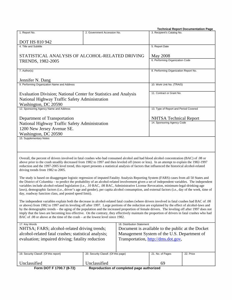
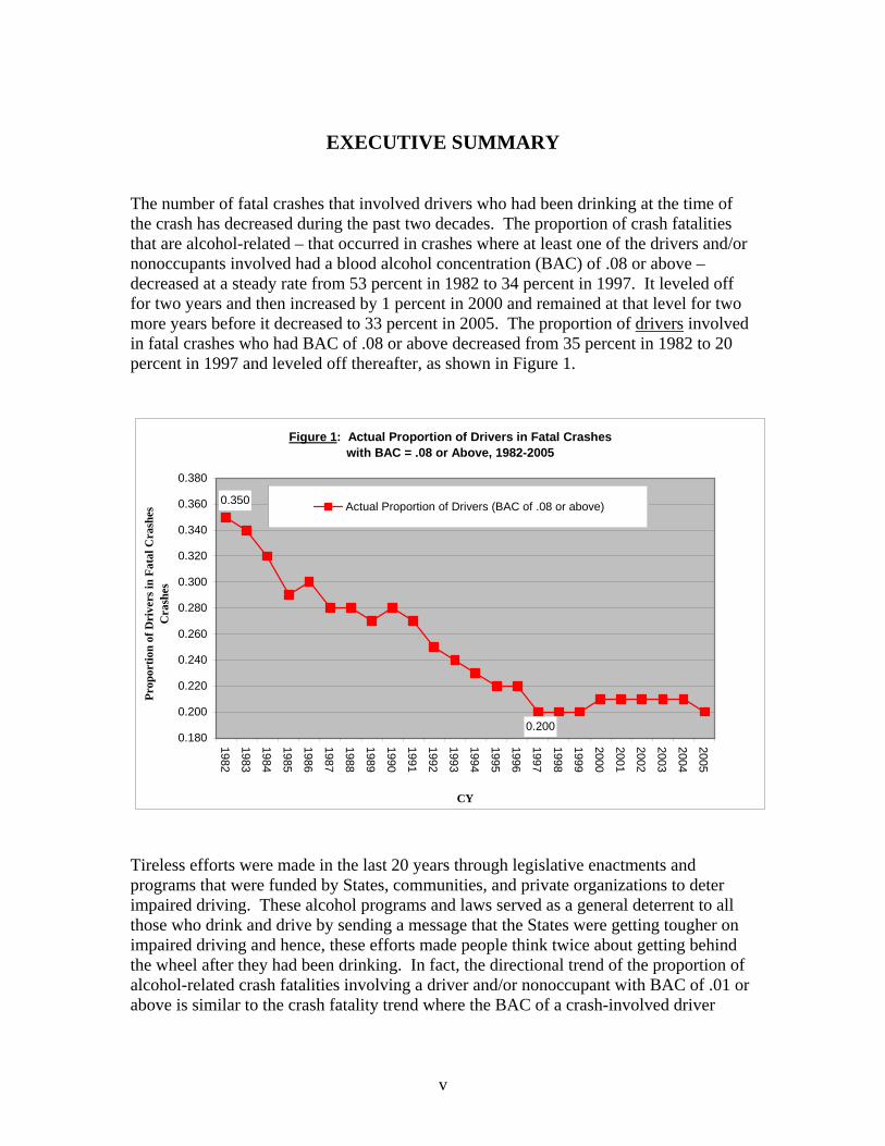
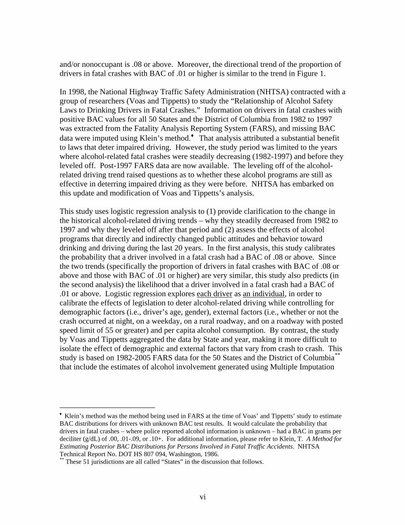
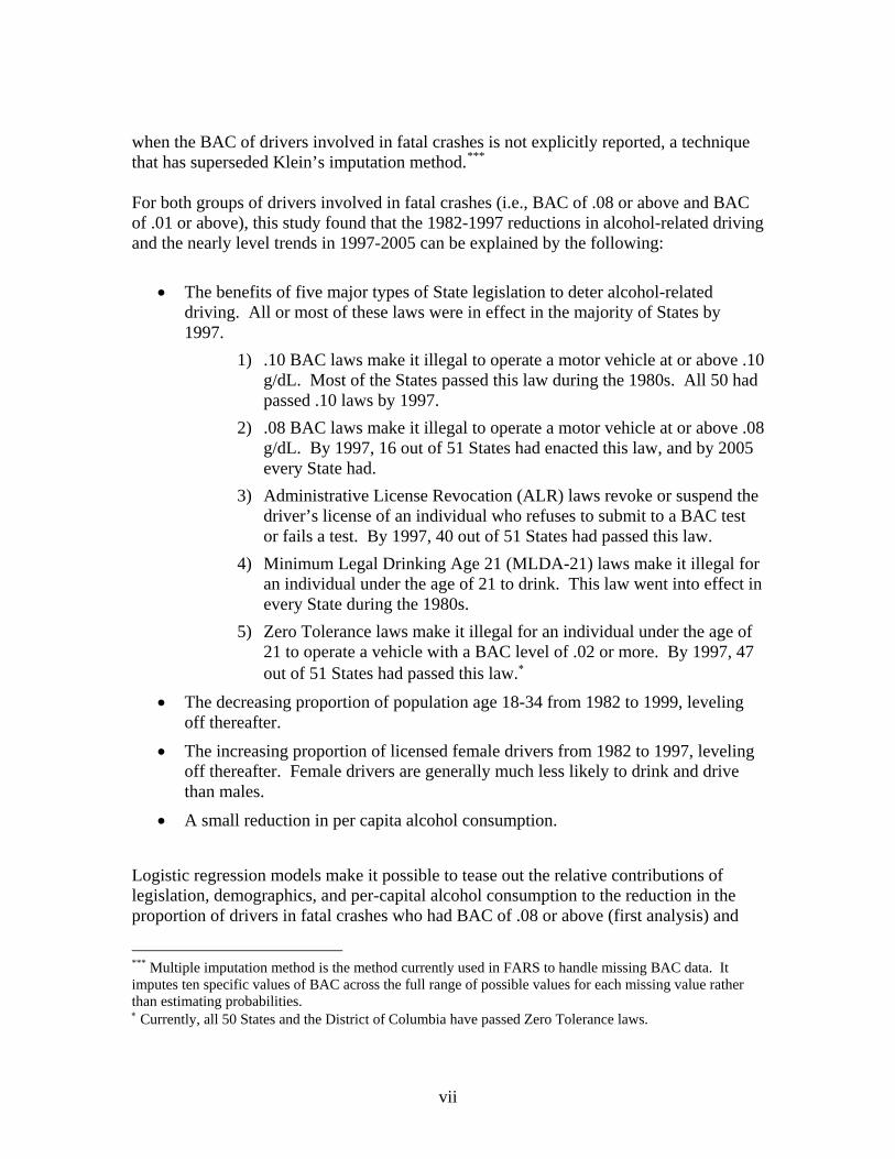
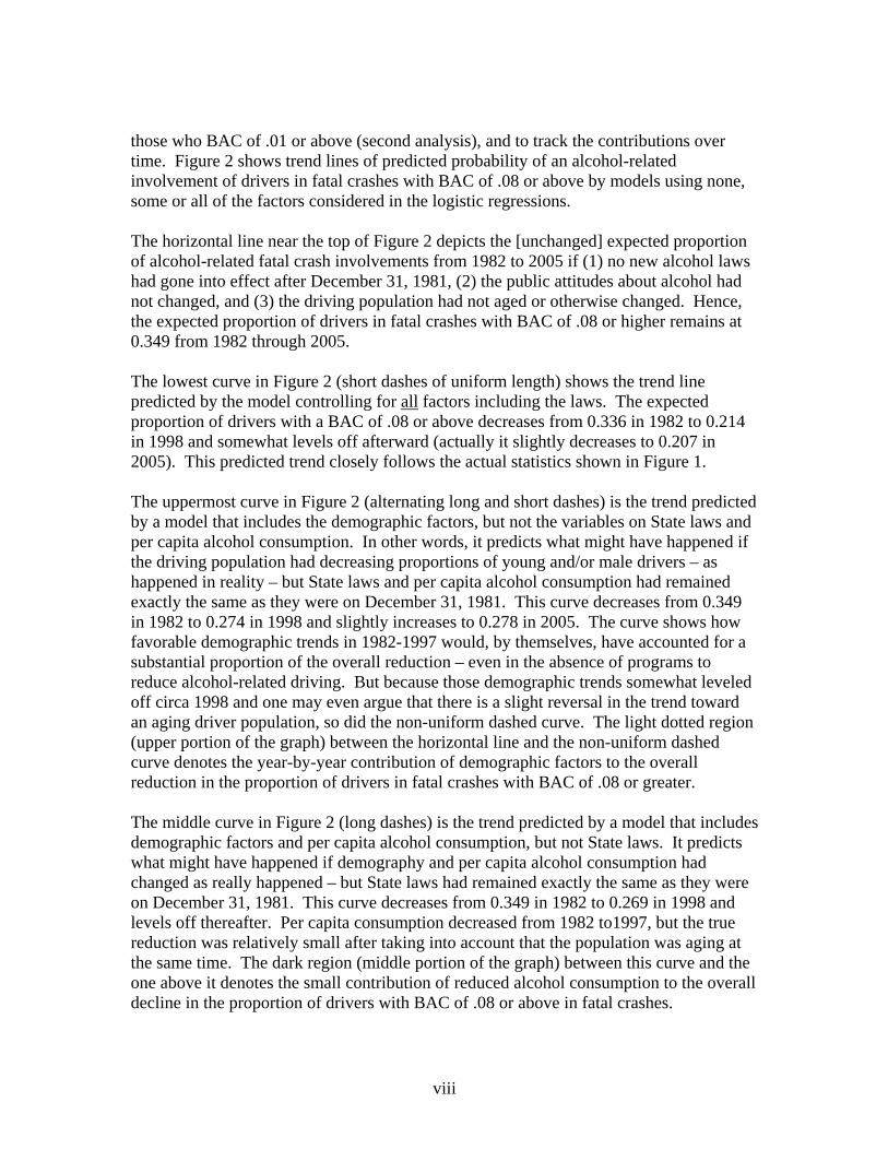
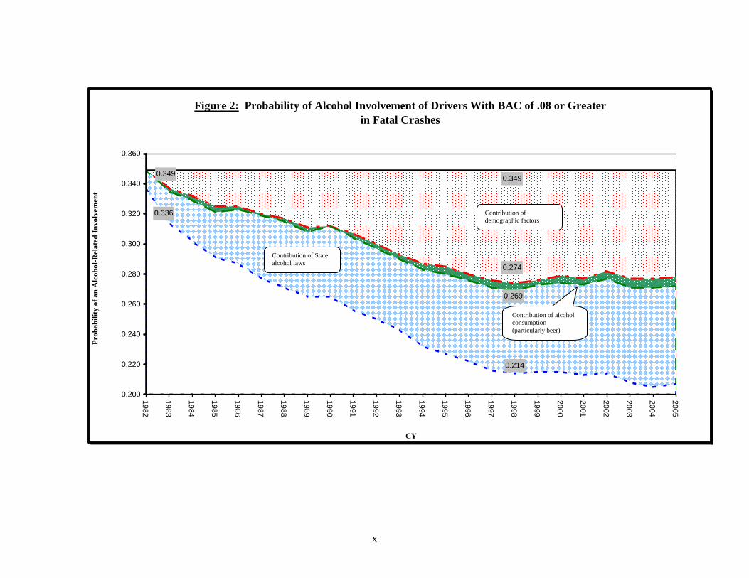
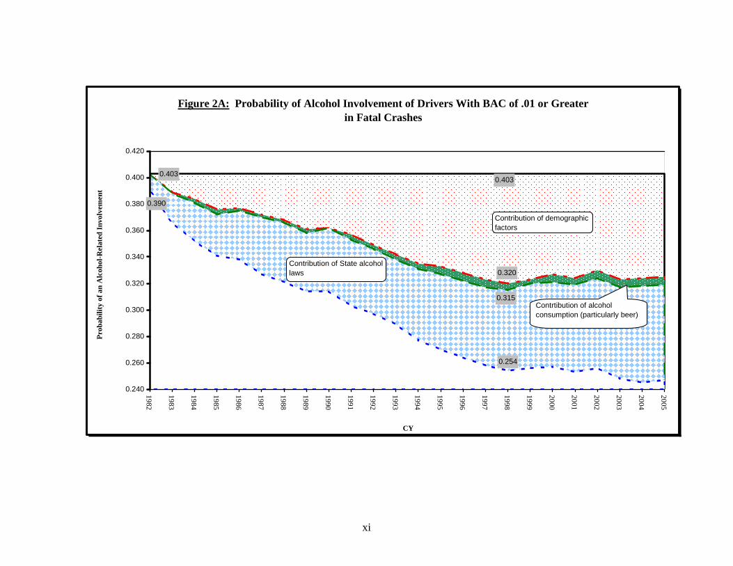
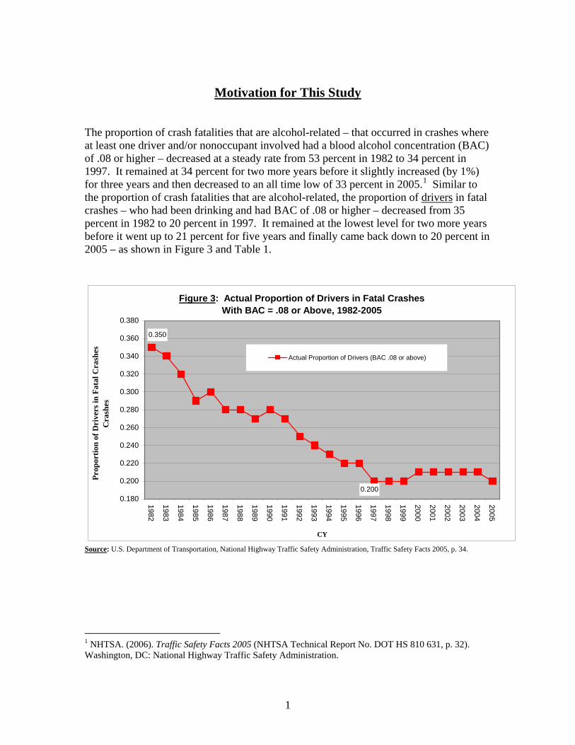
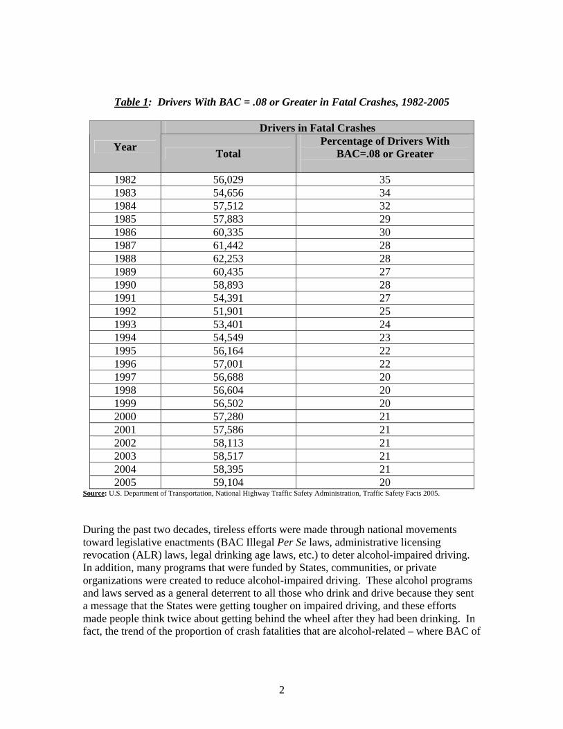