state-space estimation of multi-factor models of the term ... · statistical tests con rm that the...

STATE-SPACE ESTIMATION OF MULTI-FACTOR MODELS OF THE

TERM STRUCTURE: AN APPLICATION TO GOVERNMENT OF JAMAICA BONDS

R. BRIAN LANGRIN†

ABSTRACT

This paper estimates multi-factor versions of the Vasicek (1977) and the Cox, Ingersoll and Ross (CIR 1985) models of the term structure of interest rates using zero-coupon Government of Jamaica bond prices. Statistical tests conrm that the two-factor CIR-model best accounts for the dynamics of the term structure. The empirical analysis reveal that the level of the short rate exhibits strong and smooth mean reversion and the existence of a large and signicant risk premium that increases with time to maturity. Based on estimated factor loadings, the unobserved short rate has a signicant impact on the short end of the yield curve but a relatively minimal impact on the long end.

JEL classication: C33, E43, G12

Keywords: afne term structure, state-space models, Kalman lter

† Financial Stability Department, Bank of Jamaica, Nethersole Place, P.O. Box 621, Kingston, Jamaica, W.I. Tel.: (876) 967-1880. Fax: (876) 967-4265. Email: [email protected]

R. BRIAN LANGRIN / 31

32 / BUSINESS, FINANCE & ECONOMICS IN EMERGING ECONOMIES VOL. 2, NO. 1, 2007

1.0 Introduction

The econometric estimation of the term structure of interest rates has received tremendous attention from nancial and macro-economists, particularly in the context of bond pricing.1 Based on the Expectations Theory of the term structure, the yields on long-term bonds are the expected value of risk-adjusted average future short-term yields. Hence, measurement of the term structure of interest rates allows for the extraction of information on investors’ expectations about future interest rates. Term structure measurement models have a range of applications. Specically, interpreting the empirical properties of bond yield dynamics that are provided by term structure measurement models is important for a number of purposes that include:

• Inuencing aggregate demand through monetary policy.2

The short rate is the fundamental policy instrument of the central bank, that is, central banks may shift the short end of the yield curve when adjusting their policy stance. However, movement in long-term rates has a greater inuence on aggregate demand. Thus, knowledge of yield curve dynamics provides information to the central bank on how their interest rate decisions will impact the future path of the economy.

• Risk management through the pricing and hedging of interest rate-contingent claims including caps, floors and swaptions.3 Further, value-at-risk estimates for xed

1 See, for example, Babbs and Nowman (1999), Dai and Singleton (2000) and Pearson and Sun (1994).

2 See, for example, Ang and Piazzesi (2003), Diebold, Redebusch and Aruoba (2003), Fendel (2004), Hördahl, Tristani and Vestin (2002), Piazzesi (2003) and Rudebusch and Wu (2003).

3 See, for example, Amin and Morton (1994), Buhler et. al. (1999), Driessen, Klaasen and Melenberg (2002), Canabarro (1995), Chernov and Ghysels (2000), Jagannathan et. al., (2000) and Longstaff et. al., (2001).

income portfolios can be obtained through simulating paths for the term structure.4

• Public debt management through bond issues.5 Knowledge of the dynamic properties of the yield curve provides information on the impact of scal policy on investor risk preferences and future yield expectations of bonds across maturities. Fiscal authorities can use this information when deciding the length of tenors in their financing decisions.

There has been enormous growth since the 1990s in the sovereign bond markets for emerging economies, including Jamaica. This has led to the increased importance of obtaining information concerning the term structure of emerging countries’ sovereign bond yields in order to predict the timing of possible adverse credit events in these economies. Whereas a number of studies exist that examine the term structure of specic emerging market sovereign bond yields, no known study exists for the Jamaican case. This paper estimates the two most popular versions of afne diffusion term structure models using zero-coupon Government of Jamaica (GOJ) sovereign bonds for the period 24 September 2004 to 28 July 2006. Specically, multi-factor versions of the Vasicek (1977) and the Cox, Ingersoll and Ross (CIR 1985) models of the nominal interest rate term structure are estimated using a state-space approach. This approach simultaneously integrates time series and cross-sectional GOJ sovereign yields to generate the unobservable state variables using a Kalman lter. The objective of Section 1 then, is to examine the usefulness of popular term structure models in explaining the yield curve dynamics in Jamaica in order to derive information on investor expectations as well as to accurately price GOJ bonds and hedging instruments.

4 Value-at-Risk is dened as the maximum potential loss on a portfolio for a given horizon and probability.

5 See, for example, Dai and Philippon (2004).



The next section focuses on the theoretical formulation of the Vasicek and CIR multi-factor afne models. The state space representation of the Vasicek and CIR term structure models and the Kalman lter algorithm are presented in Section 3. One to three factor versions of these models are used to explain the dynamics of the term structure of GOJ bonds for the period 24 September 2004 to 28 July 2006. The data description and empirical results are reported in Section 4. Section 5 provides a brief conclusion.

2.0 Equilibrium Multifactor Afne Models of the Term Structure

The Vasicek (1977) and CIR (1985) models fall in the class known as “equilibrium models of the term structure” and are the two most popular versions of afne diffusion term structure models. These studies represent special cases of this class of models: the Gaussian case (Vasicek) and the non-Gaussian case (CIR). Both models rely on specic assumptions about the stochastic nature of state variables to obtain information on the dynamic evolution of the term structure within an economic environment. The distinct features of these models are that the market price of risk is identied either exogenously or endogenously and the instantaneous short rate is explicitly specied as a function of unobserved state variables.6 The main difference between these models is that the short rate in the CIR model is specied as a square root process that is proportional to the level of the interest rate, unlike the Vasicek model which assumes a constant variance. This feature prevents the occurrence of negative rates under certain restrictions.7

Single-factor term-structure models describe the dynamics of the instantaneous short rate. Hence, these models can only account for parallel shifts in the yield curve. In practice, however, other factors may inuence different sections of the yield curve allowing for various

6 The market price of risk, otherwise called the Sharpe ratio, refers to the expected standardised excess rate of return above the risk-free rate from a specic zero-coupon bond.

7 See Subrahmanyam (1996) for an extensive discussion on the Vasicek and CIR models as well as other seminal term structure models.

shapes such as twists and inverse humps. Alternatively, the exibility inherent in multi-factor term-structure models allows for a wider range of possible yield curve shapes. Three-factor term-structure models are usually estimated in practice to explain the dynamics of the term structure of interest rates. The specication of three factors relies on the seminal study by Litterman and Scheinkman (1991), based on standard principle component analysis, which found that three factors corresponding to the level, curvature and slope of the yield curve explained the term structure of US Treasury bond yields in the 1980s. However, many studies have found that the inclusion of additional factors does not increase the performance of term structure models.8 Consistent with this nding, the Litterman and Scheinkman (1991) study determined that almost 90.0 per cent of the variation in US Treasury yields was driven by the variation in the rst factor.

Multifactor afne models of the term structure represent the yields of securities as afne functions of a vector of K unobservable state variables or factors, X = (X1, X2, ..., XK)’, which is governed by the following multidimensional diffusion process9

. (1)

The instantaneous short rate is given as

(2)

The factors, Xi (t), are assumed to be independently generated by the Ornstein-Uhlenbeck (O-U) process in the Vasicek (Gaussian) case represented as

8 See, for example, Chatterjee (2005).

9 A function F:ℜn → ℜ is afne if there exist some coefcients a ∈ℜ and such that F(X) = a+bT X, ∀X ∈ℜn.



dXi (t) = κi (θi - Xi (t)) dt + σi dWi (t), i = 1, ..., K (3)

and the square-root process in the CIR (non-Gaussian) case represented as (4)

where κi , θi and σi are the speed of mean reversion, long-term mean and volatility parameters, respectively, and Wi(t) denotes the independent Wiener processes under the risk-neutral pricing measure, Φ.

The nominal pricing formula for a pure discount bond with a face value of $1 maturing at T is

(5)

where Bi (T) and Ai (T), in the Vasicek model have the following forms

(6)

(7)

and where Ai (T) and Bi (T), in the CIR model have the following forms

(8)

(9)

and . The risk premium for each state variable is λiXi where the xed parameter λi is the market price of risk for the corresponding state variable and is negatively related with the risk premium.

The pricing formula for a coupon bond with a face value of $1

maturing at T with m coupons, Ci, to be paid at Ti is

with an implied yield to maturity obtained by

solving . However, φ (X,T) would not be normally

distributed given its nonlinear relationship with X (t).

3.0 The State-Space Approach to Estimate Multi-Factor Term Structure Models

A state-space approach is adopted in this paper to estimate the unknown parameters and extract the unobservable state variables. A state-space representation is a dynamic system that comprises measurement equations, which condition observed variables on unobserved or state variables, as well as transition equations, which describe the path of the state variables. This system may be expressed in a form that may be examined using the Kalman lter which originates from the engineering control literature.10 The Kalman lter is an algorithm for sequentially updating a linear projection for the system using information from the observed variables.11 The exact state-space representation for a multi-factor model with state vector X(t) is based on the assumption that is a Markov process with X(0) ~ δ (0) [X(0)] and X(t)X(t-1) ~ δ [X(t)X (t-1] where δ (0) [X(0)] and δ [X(t)X (t-1] represent the density of the initial state vector and the transition density, respectively.

3.1 The CIR (non-Gaussian) model

Consider the following CIR square-root process for the spot interest rate

(10)

10 See Duan and Simonato (1995), Babbs and Nowman (1999), Chen and Scott (2002), De Jong (1998), Geyer and Pichler (1999) and Lund (1997) for applications of the Kalman lter to term structure models.

11 See Hamilton (1994).



The change in the instantaneous short rate has a mean-reverting drift as well as a variance which is proportional to the level of the short rate. The afne drift µ(t) = κ(θ - r(t)) ensures that if (r(t) > θ r (t) < θ) then (dr(t) < 0 (dr(t)>0) should hold under the assumption. The Feller (1951) condition 2º¸ < Ã2 ensures that the process has a reecting boundary at r (t) = 0 so that the conditional variance σ2 r(t) does not collapse to zero. This condition does not allow the process to be nonstationary (i.e. κ = 0,).

The solution for nominal price of a pure discount bond with a face value of $1 maturing at T is

P (T) = A(t) exp (-B (T) r (t)) (11)

where andare matrices with individual elements depicted by equations (8) and (9), respectively. The individual elements of and are

or, in the K = 3 - factor (12)

and (13)

The limit of the yield to maturity, or the long-term yield, as the time

to maturity gets longer is .The unobservable state variables for the CIR model are distributed

conditionally as non-central X2 variates. In order to estimate the unobservable state variables, the exact transition density is substituted by a normal density X(t)X(t-1) ˜ N(µ (t)m ∑ (t)). The matrices for the conditional mean and conditional variance of for the CIR model are determined such that they are equal to the rst two moments of the exact transition density with elements dened as

(14)

and the matrix, ∑(t), has K diagonal elements

(15)

3.2 The Vasicek (Gaussian) model

Consider the following Vasicek spot interest rate O-U process

dr(t) = κ (θ - r (t)) dt + σ dW(t) (10’)

and κ > 0 is required for the process to be stationary.The solution for nominal price of a pure discount bond with a face

value of $1 maturing at T is

P(T) = A(T) exp (B(T)r(t)) (11’)



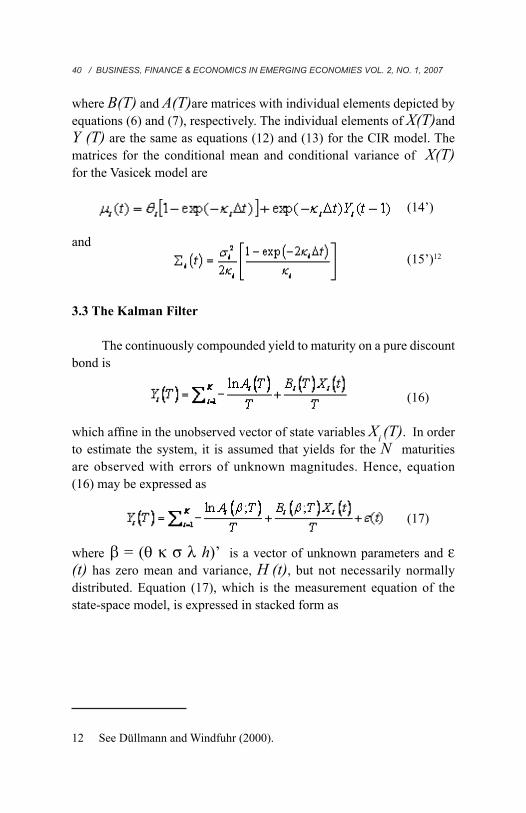
where B(T) and A(T)are matrices with individual elements depicted by equations (6) and (7), respectively. The individual elements of X(T)and Y (T) are the same as equations (12) and (13) for the CIR model. The matrices for the conditional mean and conditional variance of X(T) for the Vasicek model are

(14’)

and (15’)12

3.3 The Kalman Filter

The continuously compounded yield to maturity on a pure discount bond is

(16)

which afne in the unobserved vector of state variables Xi (T). In order to estimate the system, it is assumed that yields for the N maturities are observed with errors of unknown magnitudes. Hence, equation (16) may be expressed as

(17)

where β = (θ κ σ λ h)’ is a vector of unknown parameters and ε (t) has zero mean and variance, H (t), but not necessarily normally distributed. Equation (17), which is the measurement equation of the state-space model, is expressed in stacked form as

12 See Düllmann and Windfuhr (2000).

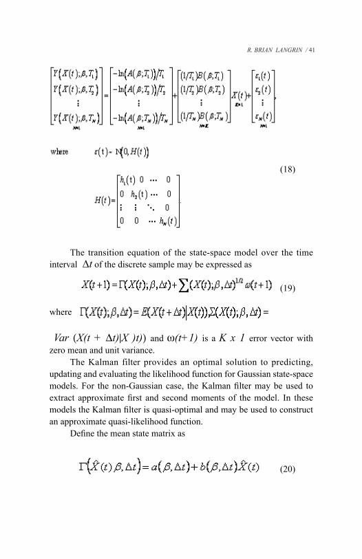
(18)

The transition equation of the state-space model over the time interval ∆t of the discrete sample may be expressed as

(19)

where

Var (X(t + ∆t)|X )t)) and ω(t+1) is a K x 1 error vector with zero mean and unit variance.

The Kalman filter provides an optimal solution to predicting, updating and evaluating the likelihood function for Gaussian state-space models. For the non-Gaussian case, the Kalman lter may be used to extract approximate rst and second moments of the model. In these models the Kalman lter is quasi-optimal and may be used to construct an approximate quasi-likelihood function.

Dene the mean state matrix as

(20)



and the state covariance matrix as

(21)

where X (t) = E (X (t) | Ω (t)), represents the information available at time t and a(.) and b(.) are K x 1 and K x K matrices, respectively.

Equations (18) and (19) describe the state space representation.

The Kalman lter provides optimal estimates, , of the state

variables given information at time t + 1. The conditional mean and

variance of may be expressed as

(22)

and

(23)

Given is afne in X(t) and

and using the law of iterated

expectations

(24)

Equations (22) and (24) are referred to as the prediction step.The second step in calculating the Kalman lter involves updating

the estimation from the prediction step given the arrival of new informa-tion based on actual observations, Y(t). Hence, the optimal estimates of the state vector and state covariance matrix are given by

(25)

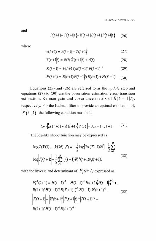
and (26)

where (27)

(28)

(29)

(30)

Equations (25) and (26) are referred to as the update step and equations (27) to (30) are the observation estimation error, transition estimation, Kalman gain and covariance matrix of R(t + 1|t), respectively. For the Kalman lter to provide an optimal estimation of,

the following condition must hold

(31) The log-likelihood function may be expressed as

(32)

with the inverse and determinant of Fi (t+1) expressed as

(33)



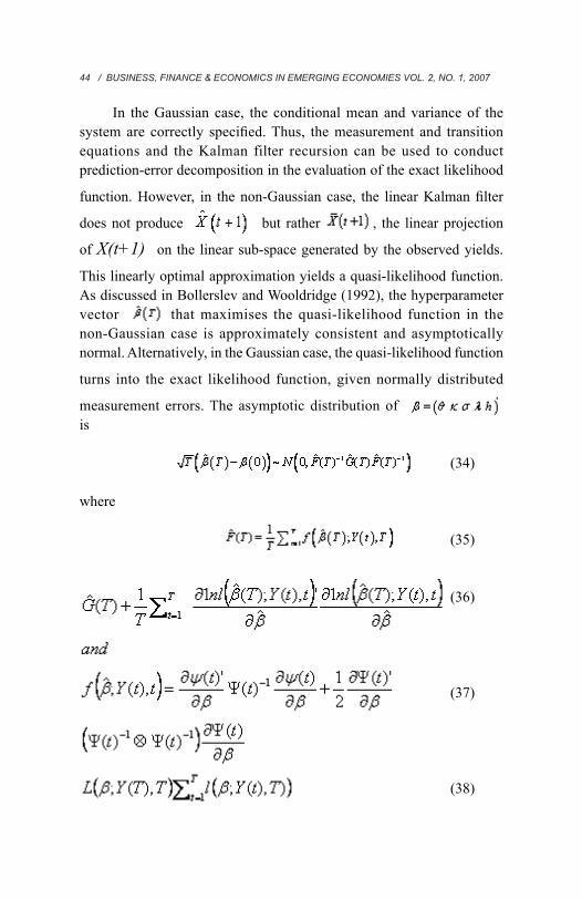
In the Gaussian case, the conditional mean and variance of the system are correctly specied. Thus, the measurement and transition equations and the Kalman filter recursion can be used to conduct prediction-error decomposition in the evaluation of the exact likelihood

function. However, in the non-Gaussian case, the linear Kalman lter

does not produce but rather , the linear projection

of X(t+1) on the linear sub-space generated by the observed yields.

This linearly optimal approximation yields a quasi-likelihood function. As discussed in Bollerslev and Wooldridge (1992), the hyperparameter vector that maximises the quasi-likelihood function in the non-Gaussian case is approximately consistent and asymptotically normal. Alternatively, in the Gaussian case, the quasi-likelihood function

turns into the exact likelihood function, given normally distributed

measurement errors. The asymptotic distribution of is

(34)

where

(35)

(36)

(37)

(38)

where Ψ and Ψ are the conditional mean and variance functions from the linear Kalman lter.13

4.0 Estimation Results of Multi-factor Models

Term structure models were originally estimated with either time series bond yields or a cross-section of bond yield over different maturities. The time series approach incorporates the intertemporal dynamics of the term structure but not cross-section information.14 However, to ensure the model is arbitrage free, a range of maturities should be included in the estimation. The cross-section approach which uses bond yield data across maturities at a point in time has the drawback that the parameters can be unstable over different points in time.15 Hence, the incorporation of both time series and cross-section data in empirical tests of the term structure allows for the proper use of information from both dimensions in order to obtain more accurate parameter estimates.16 Nevertheless, a main drawback of time series/cross-section models of the term structure is that if the number of maturities is larger than the number of factors, the model will be under-identied. In order to circumvent this problem, this paper follows the approach of most term-structure models that rely on panel data which add Gaussian measurement errors

13 See Duan and Simonato (1998).

14 Examples of recent term structure models that rely on time series data include: Anderson and Lund (1997), Brenner, Harjes and Kroner (1996), Broze, Scaillet and Zakoian (1995) and Chan, Karolyi, Longstaff and Sanders (1992).

15 Examples of recent term structure models that rely on cross-section data include: Brown and Dybvig (1986), Brown and Schaefer (1994) and De Munnik and Shotman (1994).

16 Examples of recent term structure models that incorporate both times series and cross-section data include: Babbs and Nowman (1999), Ball and Torous (1996), Chatterjee (2005), Chen and Scott (1995), De Jong (2000), Duan and Simonato (1995), Geyer and Pichler (1996), Gibbons and Ramaswamy (1993), Jegadeesh and Pennacchi (1996), Lund (1997), Pearson and Sun (1994), and Pennacchi (1991).



when estimating the relationship between the maturity yields and the unobserved state factors to obtain consistent parameters. The inclusion of measurement errors is consistent with the existence of market regularities such as bid-ask spreads and non-synchronous trading.

4.1 Data Description

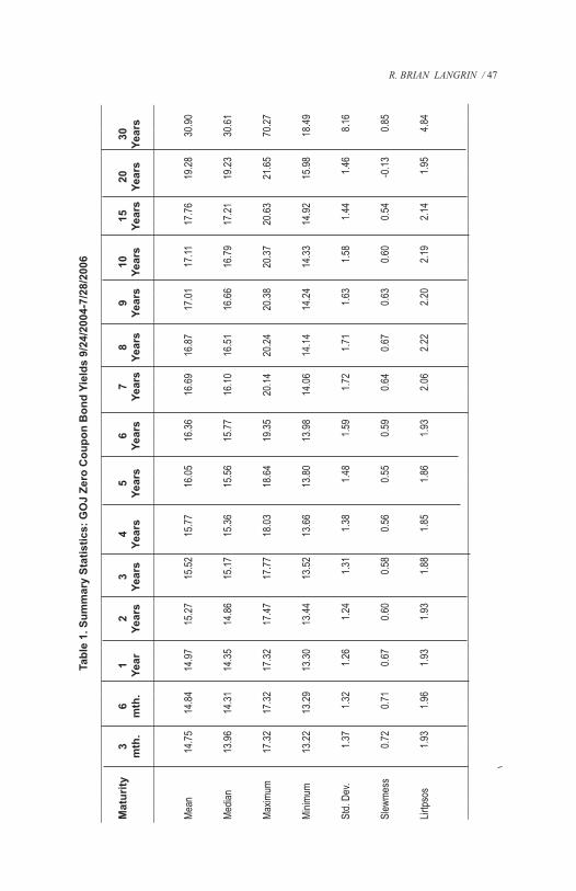
The data used in the empirical study consist of daily zero coupon GOJ domestic bond yields from 24 September 2004 to 28 July 2006 obtained from Bloomberg. In particular, the panel data set covers 435 observations and N=15 interest rates. The maturities included 0.25-, 0.5-, 1-, 2-, 3-, 4-, 5-, 6-, 7-, 8-, 9-, 10-, 15-, 20- and 30-year tenors.

The average yield per maturity over the sample period indicates that, on average, the GOJ zero coupon term-structure is upward sloping (see Table 1). The average spread or premium between the 3-month and 30-year spot rates is approximately 1,500 basis points. This signicant risk premium of 8.0 per cent demanded by investors is likely to be caused by unfavourable GOJ debt ratios. The volatility of the spot rates is greatest at the 30-year maturity and lowest at the 3-month to 4-year maturities. This is inconsistent with expectations of greater volatility at the shorter maturities which may be due to greater uncertainty regarding the riskiness of GOJ bonds. The skewness and kurtosis parameters indicate that the distributions are not normal across maturities.17 The skewness coefcient of all yields, except the 20-year yield, is greater than zero, indicating a lower downside risk relative to the normal distribution. The kurtosis values below 3 for all yields, apart from the 30-year maturity, implies lower losses when compared to the normal distribution.

The zero-coupon yields on the GOJ bonds are highly correlated (>80.0 per cent) across all maturities, abstracting from the 20- and 30-year maturities which exhibit much lower correlation coefcients (see Table 2). For the most part, the correlations are close to perfect

17 The skewness and kurtosis of the Normal distribution is 0 and 3, respectively.

Tabl

e 1.

Sum

mar

y St

atis

tics:

GO

J Ze

ro C

oupo

n B

ond

Yiel

ds 9

/24/

2004

-7/2

8/20

06__

____

____

____

____

____

____

____

____

____

____

____

____

____

____

____

____

____

____

____

____

____

____

____

____

____

____

____

____

____

____

____

____

____

____

____

__

Mat

urity

3

6

1

2

3

4

5

6

7

8

9

10

15

20

30

m

th.

m

th.

Y

ear

Y

ears

Ye

ars

Ye

ars

Year

s

Yea

rs

Ye

ars

Ye

ars

Y

ears

Ye

ars

Y

ears

Ye

ars

Ye

ars

____

____

____

____

____

____

____

____

____

____

____

____

____

____

____

____

____

____

____

____

____

____

____

____

____

____

____

____

____

____

____

____

____

____

____

____

Mean

14.75

1

4.84

1

4.97

15.27

15.52

15.77

16.0

5

16

.36

1

6.69

16

.87

17

.01

17

.11

17

.76

1

9.28

3

0.90

Media

n

13.96

1

4.31

1

4.35

14.86

15.17

15.36

15.5

6

15

.77

1

6.10

16

.51

16

.66

16

.79

17

.21

1

9.23

3

0.61

Maxim

um

1

7.32

1

7.32

1

7.32

17.47

17.77

18.03

18.6

4

19

.35

2

0.14

20

.24

20

.38

20

.37

20

.63

2

1.65

7

0.27

Minim

um

13.22

1

3.29

1

3.30

13.44

13.52

13.66

13.8

0

13

.98

1

4.06

14

.14

14

.24

14

.33

14

.92

1

5.98

1

8.49

Std.

Dev.

1.3

7

1.3

2

1.2

6

1

.24

1

.31

1

.38

1.48

1.59

1.7

2

1.71

1.63

1.58

1.44

1.4

6

8.1

6

Slew

mess

0.7

2

0.7

1

0.6

7

0

.60

0

.58

0

.56

0.55

0.59

0.6

4

0.67

0.63

0.60

0.54

-0.1

3

0.8

5

Lirtps

os

1.9

3

1.9

6

1.9

3

1

.93

1

.88

1

.85

1.86

1.93

2.0

6

2.22

2.20

2.19

2.14

1.9

5

4.8

4

____

____

____

____

____

____

____

____

____

____

____

____

____

____

____

____

____

____

____

____

____

____

____

____

____

____

____

____

____

____

____

____

____

____

____

____


48 / BUSINESS, FINANCE & ECONOMICS IN EMERGING ECONOMIES VOL. 2, NO. 1, 2007Ta

ble

2. C

orre

latio

n M

atrix

: GO

J Ze

ro C

oupo

n B

ond

Yiel

ds 9

/24/

2004

- 7/

28/2

006

____

____

____

____

____

____

____

____

____

____

____

____

____

____

____

____

____

____

____

____

____

____

____

____

____

____

____

____

____

____

____

____

____

____

_

3

6

1

2

3

4

5

6

7

8

9

10

15

20

3

0

Mth

M

th

Ye

ar

Yea

r

Ye

ar

Yea

r

Year

Year

Y

ear

Y

ear

Ye

ar

Ye

ar

Ye

ar

Ye

ar

Year

____

____

____

____

____

____

____

____

____

____

____

____

____

____

____

____

____

____

____

____

____

____

____

____

____

____

____

____

____

____

____

____

____

___

3-Mo

nth

1.00

0

.98

0.9

6

0.9

3

0

.92

0.

92

0.9

3

0

.93

0

.93

0.9

1

0.9

0

0.

90

0.9

2

0.81

0

.84

6-Mo

nth

1.00

0

.99

0

.95

0

.94

0.

94

0.9

5

0

.94

0

.94

0.9

2

0.9

1

0.

91

0.9

3

0.83

0

.48

1-Ye

ar

1.00

0.99

0.98

0.98

0.98

0.97

0.96

0.95

0.94

0.94

0.95

0

.83

0.46

2-Ye

ar

1.00

1.00

1.00

0.99

0.98

0.97

0.97

0.96

0.96

0.96

0

.79

0.39

3-Ye

ar

1.0

0

1.0

0

0.9

9

0

.98

0

.97

0.9

7

0.9

6

0.

96

0.9

6

0.79

0

.38

4-Ye

ar

1.

00

1.0

0

0

.99

0

.98

0.9

8

0.9

7

0.

97

0.9

7

0.81

0

.41

5-Ye

ar

1

.00

1.00

0.99

0.99

0.98

0.98

0.98

0

.82

0.43

6-Ye

ar

1.00

1.00

0.99

0.99

0.99

0.99

0

.83

0.45

7-Ye

ar

1.00

1.00

0.99

0.99

0.99

0

.83

0.46

8-Ye

ar

1.00

1.00

1.00

0.99

0

.80

0.43

9-Ye

ar

1.00

1.00

0.98

0

.78

0.41

10-Y

ear

1.0

0

0.9

8

0.79

0

.41

15-Y

ear

1.0

0

0.89

0

.52

20-Y

ear

1.0

0

0.71

30-Y

ear

1.00

____

____

____

____

____

____

____

____

____

____

____

____

____

____

____

____

____

____

____

____

____

____

____

____

____

____

____

____

____

____

____

____

____

___

between yields on maturities up to one year apart. As the number of years increases between maturities, these pair-wise correlation coefcients decline, suggesting the use of a multi-factor term structure model.

4.2 Empirical Results

One-, two-, and three-factor Vasicek and CIR models are estimated to obtain the parameter estimates of λ, κ, θ and σ, the standard deviation estimates of the N measurement errors, √hi, as well as the values for the log-likelihood and Akaike Information Criterion (AIC)18

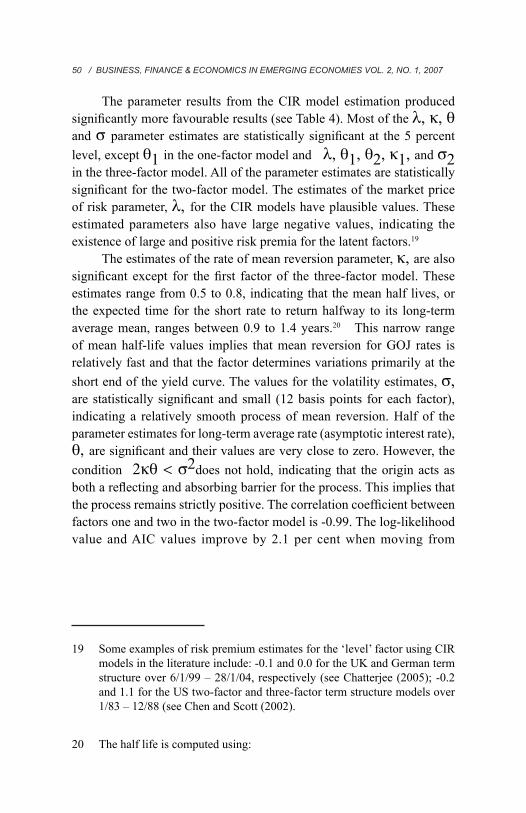
(see Tables 3 and 4; standard errors are shown in italics).The results for the Vasicek model indicate that all of the λ, θ and

parameters are statistically insignicant at the 5.0 per cent level (see Table 3). In addition, the standard errors are generally very large and in most cases increase signicantly as the number of factors increases. The results are mixed for the κ parameters. The κ parameters are statistically signicant in the two- and three-factor models but not signicant in the one-factor model. All of the estimated standard deviation parameters for the measurement errors are statistically signicant. The log-likelihood values show strong increases as the number of factors increases. However, only one of the 15 estimated standard deviation parameters for the measurement errors displays a consistent decline as the number of factors increases. The smallest standard deviations for measurement equation in the Vasicek models are 2, 3 and 0 basis points for the 5-year bond rate in the one-, two- and three-factor models, respectively. The largest standard deviations are 1,333, 1,285 and 1,195 basis points for the 30-year bond rate in the one-, two- and three-factor models, respectively. These large measurement errors suggest that the models are unable to explain a signicant portion of the 30-year yield movements.

18 The initial starting values chosen for these parameters were the same across both models. Further, the parameter estimates were robust to variations in the starting values.



The parameter results from the CIR model estimation produced signicantly more favourable results (see Table 4). Most of the λ, κ, θ and σ parameter estimates are statistically signicant at the 5 percent level, except θ1 in the one-factor model and λ, θ1, θ2, κ1, and σ2 in the three-factor model. All of the parameter estimates are statistically signicant for the two-factor model. The estimates of the market price of risk parameter, λ, for the CIR models have plausible values. These estimated parameters also have large negative values, indicating the existence of large and positive risk premia for the latent factors.19

The estimates of the rate of mean reversion parameter, κ, are also signicant except for the rst factor of the three-factor model. These estimates range from 0.5 to 0.8, indicating that the mean half lives, or the expected time for the short rate to return halfway to its long-term average mean, ranges between 0.9 to 1.4 years.20 This narrow range of mean half-life values implies that mean reversion for GOJ rates is relatively fast and that the factor determines variations primarily at the short end of the yield curve. The values for the volatility estimates, σ, are statistically signicant and small (12 basis points for each factor), indicating a relatively smooth process of mean reversion. Half of the parameter estimates for long-term average rate (asymptotic interest rate), θ, are signicant and their values are very close to zero. However, the condition 2κθ < σ2does not hold, indicating that the origin acts as both a reecting and absorbing barrier for the process. This implies that the process remains strictly positive. The correlation coefcient between factors one and two in the two-factor model is -0.99. The log-likelihood value and AIC values improve by 2.1 per cent when moving from

19 Some examples of risk premium estimates for the ‘level’ factor using CIR models in the literature include: -0.1 and 0.0 for the UK and German term structure over 6/1/99 – 28/1/04, respectively (see Chatterjee (2005); -0.2 and 1.1 for the US two-factor and three-factor term structure models over 1/83 – 12/88 (see Chen and Scott (2002).

20 The half life is computed using:

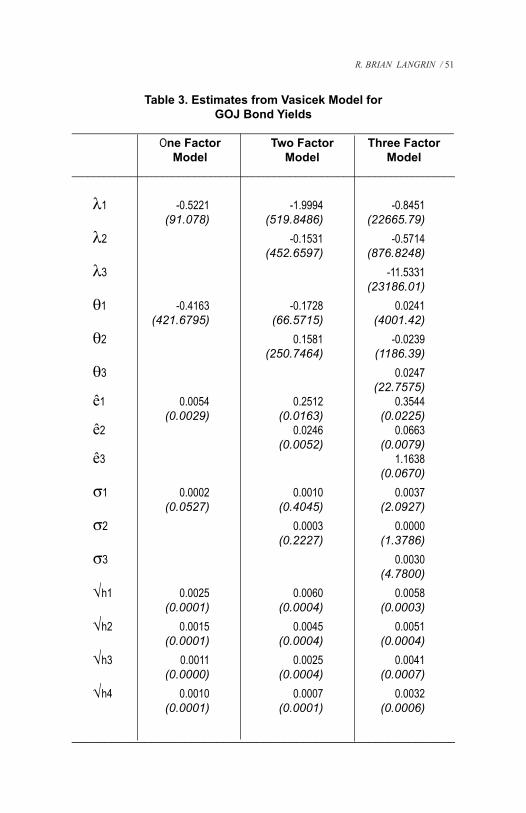
Table 3. Estimates from Vasicek Model forGOJ Bond Yields

______________________________________________________________________ One Factor Two Factor Three Factor Model Model Model________________________________________________________________________ λ1 -0.5221 -1.9994 -0.8451 (91.078) (519.8486) (22665.79) λ2 -0.1531 -0.5714 (452.6597) (876.8248) λ3 -11.5331 (23186.01) θ1 -0.4163 -0.1728 0.0241 (421.6795) (66.5715) (4001.42) θ2 0.1581 -0.0239 (250.7464) (1186.39) θ3 0.0247 (22.7575) ê1 0.0054 0.2512 0.3544 (0.0029) (0.0163) (0.0225) ê2 0.0246 0.0663 (0.0052) (0.0079) ê3 1.1638 (0.0670) σ1 0.0002 0.0010 0.0037 (0.0527) (0.4045) (2.0927) σ2 0.0003 0.0000 (0.2227) (1.3786) σ3 0.0030 (4.7800) √h1 0.0025 0.0060 0.0058 (0.0001) (0.0004) (0.0003) √h2 0.0015 0.0045 0.0051 (0.0001) (0.0004) (0.0004) √h3 0.0011 0.0025 0.0041 (0.0000) (0.0004) (0.0007) √h4 0.0010 0.0007 0.0032 (0.0001) (0.0001) (0.0006) __________________________________________________________



Table 3. Estimates from Vasicek Model forGOJ Bond Yields - Cont’d

_______________________________________________________________________ One Factor Two Factor Three Factor Model Model Model______________________________________________________________________ √h5 0.0006 0.0010 0.0026 (0.0001) (0.0002) (0.0015) √h6 0.0004 0.0008 0.0015 (0.0001) (0.0002) (0.0011) √h7 0.0002 0.0003 0.0000 (0.0001) (0.0001) (0.0000) √h8 0.0009 0.0012 0.0017 (0.0003) (0.0005) (0.0010) √h9 0.0022 0.0027 0.0036 (0.0007) (0.0010) (0.0021) √h10 0.0021 0.0024 0.0036 (0.0005) (0.0006) (0.0017) √h11 0.0023 0.0023 0.0033 (0.0005) (0.0005) (0.0011) √h12 0.0027 0.0024 0.0033 (0.0005) (0.0004) (0.0006) √h13 0.0046 0.0052 0.0069 (0.0011) (0.0013) (0.0016) √h14 0.0091 0.0098 0.0089 (0.0011) (0.0014) (0.0009) √h15 0.1333 0.1285 0.1195 (0.0059) (0.0052) (0.0041) LogL 26 319.33 28 331.25 29 712.18 AIC -120.9164 -130.1437 -136.4698_______________________________________________________________________

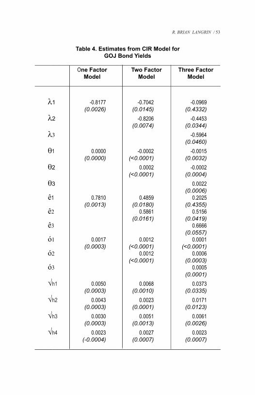
Table 4. Estimates from CIR Model forGOJ Bond Yields

______________________________________________________________________ One Factor Two Factor Three Factor Model Model Model_______________________________________________________________________ λ1 -0.8177 -0.7042 -0.0969 (0.0026) (0.0145) (0.4332) λ2 -0.8206 -0.4453 (0.0074) (0.0344) λ3 -0.5964 (0.0460) θ1 0.0000 -0.0002 -0.0015 (0.0000) (<0.0001) (0.0032) θ2 0.0002 -0.0002 (<0.0001) (0.0004) θ3 0.0022 (0.0006) ê1 0.7810 0.4859 0.2025 (0.0013) (0.0180) (0.4355) ê2 0.5861 0.5156 (0.0161) (0.0419) ê3 0.6666 (0.0557) ó1 0.0017 0.0012 0.0001 (0.0003) (<0.0001) (<0.0001) ó2 0.0012 0.0006 (<0.0001) (0.0003) ó3 0.0005 (0.0001) √h1 0.0050 0.0068 0.0373 (0.0003) (0.0010) (0.0335) √h2 0.0043 0.0023 0.0171 (0.0003) (0.0001) (0.0123) √h3 0.0030 0.0051 0.0061 (0.0003) (0.0013) (0.0026) √h4 0.0023 0.0027 0.0023 (-0.0004) (0.0007) (0.0007)__________________________________________________________



Table 4. Estimates from CIR Model forGOJ Bond Yields - Cont’d

________________________________________________________________________ One Factor Two Factor Three Factor Model Model Model_______________________________________________________________________ √h5 0.0020 0.0026 0.0005 (0.0007) (0.0008) (-0.0003) √h6 0.0012 0.0015 0.0003 (0.0004) (0.0002) (0.0001) √h7 0.0006 0.0012 0.0001 (0.0001) (0.0002) (0.0001) √h8 0.0332 0.0012 0.0007 (0.0228) (0.0003) (0.0002) √h9 0.0039 0.0016 0.0015 (0.0018) (0.0004) (0.0005) √h10 0.0038 0.0015 0.0012 (0.0017) (0.0002) (0.0001) √h11 0.0034 0.0016 0.0020 (0.0012) (0.0004) (0.0002) “√h12 0.0033 0.0010 0.1165 (0.0009) (0.0002) (0.0669) √h13 0.0056 0.0086 0.0138 (0.0016) (0.0018) (0.0100) √h14 0.0106 0.0178 0.0241 (0.0015) (0.0028) (0.0109) √h15 0.1437 0.1450 0.1325 (0.0072) (0.0120) (0.0064) LogL 25 531.71 26 068.27 24 076.15 AIC -117.2952 -119.7392 -110.557_______________________________________________________________________

the one-factor model to the two-factor model but deteriorate notably (-7.6 per cent) when moving to the three-factor model.21 This is taken as evidence that the two-factor model out-performs the one- and three-factor models.

Two of the 15 estimated standard deviation parameters for the measurement errors tend to zero as the number of factors increases. The smallest standard deviations for measurement equation in the CIR models are 6 and 1 basis points for the 5-year bond rate in the one- and three-factor models, respectively, and 10 basis points for the 10-year bond in the two-factor model. The largest standard deviations are 1,437, 1,450 and 1,325 basis points for the 30-year bond rate in the one-, two- and three-factor models, respectively. Similar to the Vasicek models, these values are signicantly larger compared to the relatively low standard deviations for the remaining bond rates. Hence, aside from the 30-year yield, the factors explain most of the yield uctuations in the CIR models, suggesting that the 30-year yield uctuation is not adequately explained by the CIR model.

The time series evolution of the combined factors of the two-factor CIR model is compared with the evolutions of the 3-month to 20-year bond yields (see Figure 1). The combined factors are strongly correlated with these yields, suggesting that monetary policy influences these yields. The correlation coefcients between the combined factors of the two-factor CIR model and GOJ yields range from 94.0 per cent to 100.0 per cent for the 3-month to 15-year yields and 82.0 per cent for the 20-year yield. The correlation between the combined factors and the 30-year yield was signicantly lower with a value of 44.0 per cent (see Figure 2). The Kalman lter one-step ahead in-sample predicted yields and the actual yields for the two-factor CIR model are illustrated in Figure 3. There appears to be a strong positive correlation between these predicted and actual yields, particularly for the 4-year to 10-year GOJ maturity yields.

21 The likelihood ratio (LR) statistic rejects the null hypothesis that the additional factors are not jointly signicant at the 1.0 per cent level. However the LR test is unreliable in this case because it does not have the standard asymptotic χ2 distribution when the errors are not Gaussian.



Figure 1. Evolution of Combined Factors of 2-Factor CIR Model and the 3-month to 20-year Maturities

Figure 2. Evolution of Combined Factors of 2-Factor CIR Model and the 30-year Maturity

Figure 3. Actual and Predicted GOJ Yields



22 See Litterman and Scheinkman (1991).

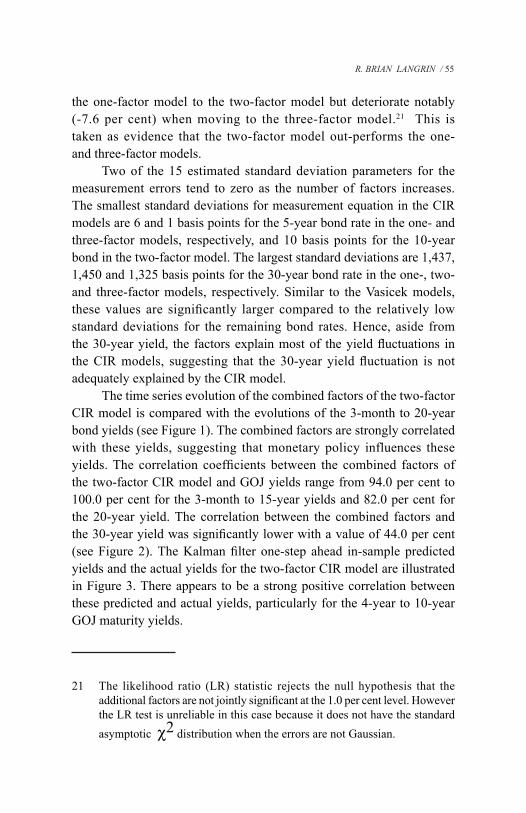
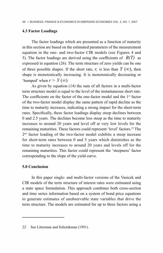
4.3 Factor Loadings

The factor loadings which are presented as a function of maturity in this section are based on the estimated parameters of the measurement equation in the one- and two-factor CIR models (see Figures 4 and 5). The factor loadings are derived using the coefcients of B(T) as expressed in equation (26). The term structure of zero yields can be one of three possible shapes. If the short rate, r, is less than Y (∞), then shape is monotonically increasing. It is monotonically decreasing or ‘humped’ when r > Y (∞)

As given by equation (14) the sum of all factors in a multi-factor term structure model is equal to the level of the instantaneous short rate. The coefcients on the factor of the one-factor model and the 1st factor of the two-factor model display the same pattern of rapid decline as the time to maturity increases, indicating a strong impact for the short-term rates. Specically, these factor loadings display steep declines between 0 and 2.5 years. The declines become less steep as the time to maturity increases to around 20 years and level off at very low levels for the remaining maturities. These factors could represent ‘level’ factors.22 The 2nd factor loading of the two-factor model exhibits a steep increase for short-term rates between 0 and 5 years which diminishes as the time to maturity increases to around 20 years and levels off for the remaining maturities. This factor could represent the ‘steepness’ factor corresponding to the slope of the yield curve.

5.0 Conclusion

In this paper single- and multi-factor versions of the Vasicek and CIR models of the term structure of interest rates were estimated using a state space formulation. This approach combines both cross-section and time series information based on a system of bond price equations to generate estimates of unobservable state variables that drive the term structure. The models are estimated for up to three factors using a

Figure 4. Factor Loading of One-Factor CIR Model

Figure 5. Factor Loadings of Two-Factor CIR Model



quasi-maximum-likelihood estimator with a Kalman lter. Fifteen bond maturities were used comprising the 0.25-, 0.5-, 1-, 2-, 3-, 4-, 5-, 6-, 7-, 8-, 9-, 10-, 15-, 20- and 30-year computed zero-coupon GOJ bond yields covering the period 24 September 2004 to 28 July 2006 to estimate the parameters of each model.

Based on the empirical results, the Vasicek models performed very poorly relative to the CIR models. Additionally, the results suggested that the 2-factor CIR model provided the best representation of the dynamics of the yield curve. Based on the factor loadings, extracted factors of the two-factor model correspond with the general level and slope of interest rates, respectively. The empirical analysis for the 2-factor model revealed that the level of the short rate exhibited strong and smooth mean reversion and indicated the existence of a large and signicant risk premium that increases with time to maturity. The values of the parameter estimates for the long-term average rate are all virtually zero. However, this is probably a result of the sample period under analysis. That is, the period corresponds to a consistent series of downward adjustments to Bank of Jamaica repurchase rates following a substantial upward adjustment of over 15,000 basis points during an episode of substantial foreign exchange market instability in 2003. The strong reversal of the short rate since 2003 could explain the dominant expectations of investors for considerable loosening of monetary policy being reected in the estimated long-term average rate.

A summary of the key ndings of this study, based on signicant estimates from two-factor CIR model is as follows:

• The short-rate (inuenced by monetary policy) exhibits rapid decline between 0 and 2.5 years which becomes less steep as the time to maturity increases to around 20 years and levels off to a very low level for the remaining bond maturities

• Risk premium parameters have large negative values, indicating the existence of a large and positive risk premia for the ‘level and ‘steepness’ factors that increases with the time to maturity of GOJ bonds

.23 See, for example, Rudebusch and Wu (2003) for an application of a ‘macro-nance’ term structure model to US Treasury yields.

• Long-run average yield parameters reveal that investors were expecting lower interest rates over the sample period

• Mean reversions for the ‘level’ and ‘steepness’ factors that drive the dynamics of GOJ yields are relatively fast and smooth, indicating relatively short lives for monetary shocks

• The ‘level’ and ‘steepness’ factors explain variations primarily at the short end of the yield curve

• The Kalman lter one-step ahead predicting yields appear

to closely track actual GOJ bond yields, particularly for the 4-year to 10-year maturity yields.

Similar to traditional research on the term structure, this study examined a ‘yields-only’ latent-factor model of the dynamics of the yield curve. Recent studies in the literature have focused on uncovering the relationship between term structure models and specic macroeconomic variables. Future research will explicitly incorporate the relationship between term structure latent factors and macroeconomic variables of interest in the Jamaica case. For example, based on estimated factor loadings, this study concluded that the unobserved short rate (related to the BOJ policy rate) has a signicant impact on the short end of the yield curve and a relatively minimal impact on the long end. Relevant observable macroeconomic variables that could be jointly incorporated with latent state variables in a state-space model of the term structure include monetary aggregates, the expected ination gap, the expected output gap, and foreign interest rates, as well as the scal decit to account for yield movements at the long end. 23



REFERENCES

Amin, K.I., and A.J. Morton. 1994. “Implied Volatility Functions in Arbitrage-Free Term Structure Models”. Journal of Financial Economics, Vol. 35, No. 2, 141-180.

Anderson, Torben G. and Jesper Lund. 1997. “Estimating Continuous-Time Stochastic Volatility Models of the Short-Term Interest Rate”. Journal of Econometrics, Vol. 72, No. 2, 343-377.

Ang, A. and M. Piazzesi. 2003. “A No-Arbitrage Vector Autoregression of Term Structure Dynamics with Macroeconomic and Latent Variables”. UCLA Working Paper.

Babbs, Simon H. and K. Ben Nowman. 1999. “Kalman Filtering of Generalized Vasicek Term Structure Models”. Journal of Financial and Quantitative Analysis, Vol. 34, No. 1, 115-130.

Ball, Clifford A. and Walter N. Torous. 1992. “Unit Roots and the Estimation of Interest Rate Dynamics”. Anderson Graduate School of Management, UCLA Working Paper.

Benninga, S. and Z. Weiner. 1999. “An Investigation of Cheapest to Deliver on Treasury Bond Futures Contracts”. Journal of Computational Finance, Vol. 2, No. 3, 39-55.

Brenner, Robin J., Richard H. Harjes, and Kenneth F. Kroner. 1996. “Another Look at Models of the Short-Term Interest Rate”. Journal of Financial and Quantitative Analysis, Vol. 31, No. 1, 85-107.

Brown, Roger H. and Stephen M. Schaefer. 1994. “The Term Structure of Real Interest Rates and the Cox, Ingersoll and Ross Model”. Journal of Financial Economics, Vol. 35, No. 1, 3-42.

Brown, Stephen and Phillip Dybvig. 1986. “The Empirical Implications of the Cox, Ingersoll, Ross Theory of the Term Structure of Interest Rates”. The Journal of Finance, Vol. 41, No. 3, 617-630.

Broze, Laurence, Olivier Scaillet and Jean-Michel Zakoian. 1995. “Testing for Continuous Time Models of the Short-Term Interest Rate”. The Journal of Empirical Finance, Vol. 2, No. 3, 199-223.

Buhler, Wolfgang, Marliese Ihrig-Homburg, Ulrivh Walter and Thomas Weber. 1999. “An Empirical Comparison of Forward-Rate and Spot-Rate Models for Valuing Interest-Rate Options”. The Journal of Finance, Vol. LIV, No. 1.

Canabarro, E. 1995. “Where Do One-Factor Interest Rate Models Fail?” Journal of Fixed Income, 31-52.

Chan, K. C., G. Andrew Karolyi, Francis A. Longstaff and Anthony B. Sanders. 1992. “An Empirical Comparison of Alternative Models of the Term Structure of Interest Rates”. The Journal of Finance, Vol. 47, No. 3, 1209-1228.

Chatterjee, Somnath. 2005. “Application of the Kalman Filter for Estimating Continuous Time Term Structure Models: The Case of UK and Germany”. University of Glasgow Working Paper.

Chen, Ren-Raw and Louis Scott. 2002. “Multifactor Cox-Ingersoll-Ross Models of the Term Structure: Estimates and Tests from a Kalman Filter Model”. Working Paper.

Chen, Ren-Raw and Louis Scott. 1993. “Maximum Likelihood Estimation for a Multifactor Equilibrium Model of the Term Structure of Interest Rates”. The Journal of Fixed Income, Vol. 3, 14-31.

Chernov, Mike and Eric Ghysels. 2000. “A Study Towards a Unied Approach to the Joint Estimation of Objective and Risk Neutral Measures for the Purpose of Options Valuation”. Journal of Financial Economics, Vol. 56, 407-458.

Cox, John C., Jonathan E. Ingersoll, Jr. and Stephen A. Ross. 2005. “A Theory of the Term Structure of Interest Rates”. Econometrica, Vol. 53, No. 2, 385-407.



Dai, Qiang and Kenneth J. Singleton. 2000. “Specication Analysis of Afne Term Structure Models”. The Journal of Finance, Vol. 55, 385-407.

Dai, Qiang and Thomas Philippon. 2004. “Fiscal Policy and the Term Structure of Interest Rates”. University of North Carolina at Chapel Hill Working Paper.

Diebold, Francis, Glenn D. Rudebusch and S. Boragan Aruoba. 2004. “The Macroeconomy and the Yield Curve: A Dynamic Latent Factor Approach”. NBER Working Paper No. W10616.

Driessen, J., Pieter Klaasen and Bertrand Melenberg. 2002. “The Performance of Multi-Factor Term Structure Models for Pricing and Hedging Caps and Swaptions”. Working Paper.

Duan J.C. and J.G. Simonato. 1999. “Estimating and Testing Exponential Afne Term Structure Models by the Kalman Filter”. Review of Quantitative Finance and Accounting Vol. 13, No. 2, 111-135.

Dülmann, Klaus and Marc Windfuhr. 2002. “Credit Spreads Between German and Italian Sovereign Bonds: Do One-Factor Affine Models Work?” Canadian Journal of Administrative Sciences, Vol. 17.

Estrella, Arturo and Mary R. Trubin. 2006. “The Yield Curve as a Leading Indicator: Some Practical Issues”. Current Issues in Economics and Finance, Federal Reserve Bank of New York Vol. 12, No. 5.

Fendel, Ralf. 2004. “Towards a Joint Characterization of Monetary Policy and the Dynamics of the Term Structure of Interest Rates”. Discussion Paper, Studies of the Economic Research Centre, Deutsche Bundesbank Vol. 24.

Geyer, Alois L. J. and Stefan Pichler. 1999. “A State-Space Approach to Estimate and Test Multifactor Cox-Ingersoll-Ross Models of the Term Structure”. The Journal of Financial Research, Vol. 32, No. 1, 107-130.

Gibbons, Michael and Krishna Ramaswamy. 1993. “A Test of the Cox, Ingersoll and Ross Model of the Term Structure”. Review of Financial Studies, Vol. 6, 619-632.

Hamilton, James D. 1994. Time Series Analysis. Princeton (NJ): Princeton University Press.

Hördahl, P., O. Tristani and D. Vestin. 2003. “A Joint Econometric Model of Macroeconomic and Term Structure Dynamics”. European Central Bank Working Paper Series, No. 405.

Jagannathan, R., A. Kaplin and S. G. Sun. 2000. “An Evaluation of Multi-Factor CIR Models Using LIBOR, Swap Rates and Cap and Swaption Prices”. Working Paper.

Jegadeesh, Narasimhan and George Pennacchi. 1996. “The Behavior of Interest Rates Implied by the Term Structure of Eurodollar Futures”. Journal of Money, Credit and Banking, Vol. 28, 426-446.

Litterman, R. and J. Scheinkman. 1991. “Common Factors Affecting Bond Returns”. Journal of Fixed Income, Vol. 1, 54-61.

Longstaff, F. A., P. Santa-Clara and E. Schwartz. 2001. “The Relative Valuation of Caps and Swaptions: Theory and Empirical Evidence”. Journal of Finance, Vol. 56, No. 6, 2067-2109.

Lund, J. 1997. “Econometric Analysis of Continuous-Time Arbitrage-Free Models of the Term Structure of Interest Rates”. Department of Finance Working Paper, The Aarhus School of Business.



Pearson, N.D., and T.S. Sun. 1994. “Exploiting the Conditional Density in Estimating the Term Structure: An Application to the Cox-Ingersoll-Ross Model”. Journal of Finance, Vol. 49, 1279-1304.

Pennacchi, George G. 1991. Identifying the Dynamics of Real Interest Rates and Inflation: Evidence Using Survey Data”. Review of Financial Studies Vol. 4, No. 1, 53-86.

Piazzesi, M. 2003. “Bond Yields and the Federal Reserve”. Working Paper.

Rudebusch, Glenn D. and Tao Wu. 2003. “A Macro-Finance Model of the Term Structure, Monetary Policy and the Economy”. Working Papers in Applied Economic Theory, Federal Reserve Bank of San Francisco.

Subrahmanyam, Marti G. 1996. “The Term Structure of Interest Rates: Alternative Approaches and Their Implications for the Valuation of Contingent Claims”. The Geneva Papers on Risk and Insurance Theory Vol. 21, 7-28.

Vasicek, Oldrich. 1977. “An Equilibrium Characterization of the Term Structure”. Journal of Financial Economics, Vol. 5, No. 2, 177-188.

state-space estimation of multi-factor models of the term ... · statistical tests con rm that the...

Documents