Transactions of the ASAE

Vol. 48(3): 1101−1113 2005 American Society of Agricultural Engineers ISSN 0001−2351 1101

ESTIMATION OF LONG-TERM SOIL MOISTURE USING ADISTRIBUTED PARAMETER HYDROLOGIC MODEL AND

VERIFICATION USING REMOTELY SENSED DATA

B. Narasimhan, R. Srinivasan, J. G. Arnold, M. Di Luzio

ABSTRACT. Soil moisture is an important hydrologic variable that controls various land surface processes. In spite of itsimportance to agriculture and drought monitoring, soil moisture information is not widely available on a regional scale.However, long-term soil moisture information is essential for agricultural drought monitoring and crop yield prediction. Thehydrologic model Soil and Water Assessment Tool (SWAT) was used to develop a long-term record of soil water at a fine spatial(16 km2) and temporal (weekly) resolution from historical weather data. The model was calibrated and validated using streamflow data. However, stream flow accounts for only a small fraction of the hydrologic water balance. Due to the lack ofmeasured evapotranspiration or soil moisture data, the simulated soil water was evaluated in terms of vegetation response,using 16 years of normalized difference vegetation index (NDVI) derived from NOAA-AVHRR satellite data. The simulatedsoil water was well-correlated with NDVI (r as high as 0.8 during certain years) for agriculture and pasture land use types,during the active growing season April-September, indicating that the model performed well in simulating the soil water. Thestudy provides a framework for using remotely sensed NDVI to verify the soil moisture simulated by hydrologic models in theabsence of auxiliary measured data on ET and soil moisture, as opposed to just the traditional stream flow calibration andvalidation.

Keywords. Drought, Evapotranspiration, NDVI, Soil moisture, SWAT, Texas.

oil moisture is an important hydrologic variable thatcontrols various land surface processes. The term“soil moisture” generally refers to the temporarystorage of precipitation in the top 1 to 2 m of soil ho-

rizon. Although only a small percentage of total precipitationis stored in the soil after accounting for evapotranspiration(ET), surface runoff, and deep percolation, soil moisture re-serve is critical for sustaining agriculture, pasture, and forest-lands. Given the fact that precipitation is a random event, soilmoisture reserve is essential for regulating the water supplyfor crops between precipitation events. Soil moisture is an in-tegrated measure of several state variables of climate andphysical properties of land use and soil. Hence, it is a goodmeasure for scheduling various agricultural operations, cropmonitoring, yield forecasting, and drought monitoring.

In spite of its importance to agriculture and droughtmonitoring, soil moisture information is not widely available

Article was submitted for review in December 2004; approved forpublication by the Soil & Water Division of ASAE in April 2005.

The authors are Balaji Narasimhan, ASAE Member Engineer,Post-Doctoral Research Associate, and Raghavan Srinivasan, ASAEMember, Director and Professor, Spatial Sciences Laboratory, TexasAgricultural Experiment Station, Texas A&M University, College Station,Texas; Jeffrey G Arnold, Agricultural Engineer, USDA-ARS GrasslandSoil and Water Research Laboratory, Temple, Texas; and Mauro Di Luzio,Assistant Research Scientist, Blackland Research and Extension Center,Texas Agricultural Experiment Station, Texas A&M University, Temple,Texas. Corresponding author: Balaji Narasimhan, Spatial SciencesLaboratory, Texas Agricultural Experiment Station, Texas A&MUniversity, 1500 Research Parkway Suite B223, College Station, TX77845: phone: 979-845-7201; fax: 979-862-2607; e-mail: balaji@neo.tamu.edu.

on a regional scale. This is partly because soil moisture ishighly variable both spatially and temporally and is thereforedifficult to measure on a large scale. The spatial and temporalvariability of soil moisture is due to heterogeneity in soilproperties, land cover, topography, and non-uniform dis-tribution of precipitation and ET.

On a local scale, soil moisture is measured using variousinstruments, such as tensiometers, TDR (time domainreflectometry) probes, neutron probes, gypsum blocks, andcapacitance sensors. The field measurements are oftenwidely spaced, and the averages of these point measurementsseldom yield soil moisture information on a watershed scaleor regional scale due to the heterogeneity involved.

In this regard, microwave remote sensing is emerging asa better alternative for getting a reliable estimate of soilmoisture on a regional scale. With current microwavetechnology, it is possible to estimate soil moisture accuratelyonly in the top 5 cm of the soil (Engman, 1991). However, theroot systems of most agricultural crops extract soil moisturefrom 20 to 50 cm at the initial growth stages and extenddeeper as the growth progresses. Further, the vegetativecharacteristics, soil texture, and surface roughness stronglyinfluence the microwave signals and introduce uncertainty inthe soil moisture estimates (Jackson et al., 1996).

Field-scale data and remotely sensed soil moisture dataare available for only a few locations and are lacking for largeareas and for multiyear periods. However, long-term soilmoisture information is essential for agricultural droughtmonitoring and crop yield prediction (Narasimhan, 2004).Keyantash and Dracup (2002) also noted the lack of anational soil moisture monitoring network in spite of itsusefulness for agricultural drought monitoring.

S

1102 TRANSACTIONS OF THE ASAE

LONG-TERM SOIL MOISTURE MODELINGA possible alternative for obtaining long-term soil

moisture information is to use historical weather data.Long-term weather data, such as precipitation and tempera-ture, are widely available and can be used with spatiallydistributed hydrologic models to simulate soil moisture. Veryfew modeling studies conducted in the past were aimed atusing hydrologic models for the purpose of monitoring soilmoisture and drought.

Palmer (1965) used a simple two-layer lumped parameterwater balance model to develop the Palmer Drought SeverityIndex (PDSI). The model is based on monthly time step anduses monthly precipitation and temperature as weather inputsand average water holding capacity for the entire climaticdivision (7000 to 100,000 km2). From these inputs, a simplelumped parameter water balance model is used to calculatevarious water balance components including ET, soil re-charge, runoff, and moisture loss from the surface layer.Akinremi and McGinn (1996) found that the water balancemodel used by Palmer (1965) did not account for snowmelt,which is significant in Canadian climatic conditions. In orderto overcome this limitation, Akinremi and McGinn (1996)used the modified Versatile Soil Moisture Budget (VB),developed by Akinremi et al. (1996). Huang et al. (1996)developed a one-layer soil moisture model to derive ahistorical record of monthly soil moisture over the entire U.S.for applications of long-range temperature forecasts. Themodel uses monthly temperature and monthly precipitationas inputs, calculates surface runoff as a simple function ofantecedent soil moisture and precipitation, and estimates ETusing the Thornthwaite method.

In all of the aforementioned studies for determining soilmoisture, the weather data are used at a coarse temporal(monthly) and spatial (several thousand km2) resolution.However, precipitation has high spatial and temporal vari-ability; hence, it is not realistic to assume a uniformdistribution of precipitation over the entire climatic division.Further, physical properties of soil, land use, and topographyare highly heterogeneous and govern the hydrologic responseon a local scale. In addition, soil moisture stress can developrapidly over a short period of time, and moisture stress duringcritical stages of crop growth can significantly affect the cropyield. For example, a 10% water deficit during the tasseling-pollination stage of corn could reduce the yield as much as25% (Hane and Pumphrey, 1984).

There are other classes of models similar to the SimpleBiosphere Model (SiB) (Sellers et al., 1986) that simulateland surface fluxes (radiation, heat, moisture) for use withinthe General Circulation Model (GCM), which handleslarge-scale climate change studies and climate forecasts overa long period of time. However, these models were developedfor a different purpose, i.e., climate forecasting on a largerscale, and are data intensive. They cannot be applied on acatchment scale due to the lack of model parameters andsub-hourly input data, primarily radiation.

Many comprehensive spatially distributed hydrologicmodels have been developed in the past decade due toadvances in hydrologic sciences, Geographical InformationSystem (GIS), and remote sensing. A good compromisewould be to select a hydrologic model that (1) takes intoaccount the major land surface processes and climaticvariables, (2) gives proper consideration to spatial variability

of soil and land use properties, (3) models crop growth androot development, and (4) uses readily available data inputs.Such a model will certainly improve our ability to monitorsoil moisture at a higher spatial and temporal resolution(Narasimhan, 2004).

Among the many hydrologic models developed in the pastdecade, the Soil and Water Assessment Tool (SWAT),developed by Arnold et al. (1998), has been used extensivelyby researchers. This is because SWAT (1) uses readilyavailable inputs for weather, soil, land, and topography,(2) allows considerable spatial detail for basin-scale model-ing, and (3) is capable of simulating crop growth and landmanagement scenarios. SWAT has been integrated withGRASS GIS (Srinivasan et al., 1998b) and with ArcView GIS(Di Luzio et al., 2002b). SWAT was applied to design theHydrologic Unit Model of the United States (HUMUS) toimprove water resources management at local and regionallevels (Srinivasan et al., 1998a). SWAT is recognized by theU.S. Environmental Protection Agency (EPA) and has beenincorporated into the EPA’s BASINS (Better AssessmentScience Integrating Point and Non-point Sources) (Di Luzioet al., 2002a). (BASINS is a multipurpose environmentalanalysis software system developed by the EPA for perform-ing watershed and water quality studies on various regionaland local scales.) In order to optimally calibrate the modelparameters, especially for large-scale modeling, an auto-cal-ibration routine has been added to SWAT (Eckhardt andArnold, 2001; Van Griensven and Bauwens, 2001). Hence,SWAT was used in this study.

The objective of this study is to develop long-term soilmoisture information, at 4 × 4 km spatial resolution andweekly temporal resolution, for selected watersheds inTexas, using the spatially distributed hydrologic modelSWAT and verify the model predictions using remotelysensed data.

METHODOLOGYSOIL AND WATER ASSESSMENT TOOL (SWAT)

SWAT is a physically based basin-scale, continuous time,distributed parameter hydrologic model that uses spatiallydistributed data on soil, land use, Digital Elevation Model(DEM), and weather data for hydrologic modeling andoperates on a daily time step. Major model componentsinclude weather, hydrology, soil temperature, plant growth,nutrients, pesticides, and land management. A completedescription of the SWAT model components (version 2000)is found in Arnold et al. (1998) and Neitsch et al. (2002). Abrief description of the SWAT hydrologic component is givenhere.

For spatially explicit parameterization, SWAT subdivideswatersheds into sub-basins based on topography, which arefurther subdivided into hydrologic response units (HRU)based on unique soil and land use characteristics. Fourstorage volumes represent the water balance in each HRU inthe watershed: snow, soil profile (0 to 2 m), shallow aquifer(2 to 20 m), and deep aquifer (>20 m). The soil profile can besubdivided into multiple layers. Soil water processes includesurface runoff, infiltration, evaporation, plant water uptake,inter (lateral) flow, and percolation to shallow and deepaquifers.

1103Vol. 48(3): 1101−1113

SWAT can simulate surface runoff using either themodified SCS curve number (CN) method (USDA-SCS,1972) or the Green and Ampt infiltration model based on aninfiltration excess approach (Green and Ampt, 1911) depend-ing on the availability of daily or hourly precipitation data,respectively. The SCS curve number method was used in thisstudy with daily precipitation data. Based on the soilhydrologic group, vegetation type, and land managementpractice, initial CN values are assigned from the SCShydrology handbook (USDA-SCS, 1972). SWAT updates theCN values daily based on changes in soil moisture.

The excess water available after accounting for initialabstractions and surface runoff, using the SCS curve numbermethod, infiltrates into the soil. A storage routing techniqueis used to simulate the flow through each soil layer. SWATdirectly simulates saturated flow only and assumes that wateris uniformly distributed within a given layer. Unsaturatedflow between layers is indirectly modeled using depthdistribution functions for plant water uptake and soil waterevaporation. Downward flow occurs when the soil water inthe layer exceeds field capacity and the layer below is notsaturated. The rate of downward flow is governed by thesaturated hydraulic conductivity. Lateral flow in the soilprofile is simulated using a kinematic storage routingtechnique that is based on slope, slope length, and saturatedconductivity. Upward flow from a lower layer to the upperlayer is regulated by the soil water to field capacity ratios ofthe two layers. Percolation from the bottom of the root zoneis recharged to the shallow aquifer.

SWAT has three options for estimating potential ET:Hargreaves, Priestley-Taylor, and Penman-Monteith. ThePenman-Monteith method (Monteith, 1965) was used in thisstudy. SWAT computes evaporation from soils and plantsseparately, as described in Ritchie (1972). Soil water

evaporation is estimated as an exponential function of soildepth and water content based on potential ET and a soilcover index based on aboveground biomass. Plant waterevaporation is simulated as a linear function of potential ET,leaf area index (LAI), root depth (from crop growth model),and soil water content.

The crop growth model used in SWAT is a simplificationof the EPIC crop model (Williams et al., 1984). A singlemodel is used for simulating both annual and perennialplants. Phenological crop growth from planting is based ondaily-accumulated heat units above a specified optimal basetemperature for each crop, and the crop biomass is accumu-lated each day based on the intercepted solar radiation untilharvest. The canopy cover, or LAI, and the root developmentare simulated as a function of heat units and crop biomass.

STUDY AREA

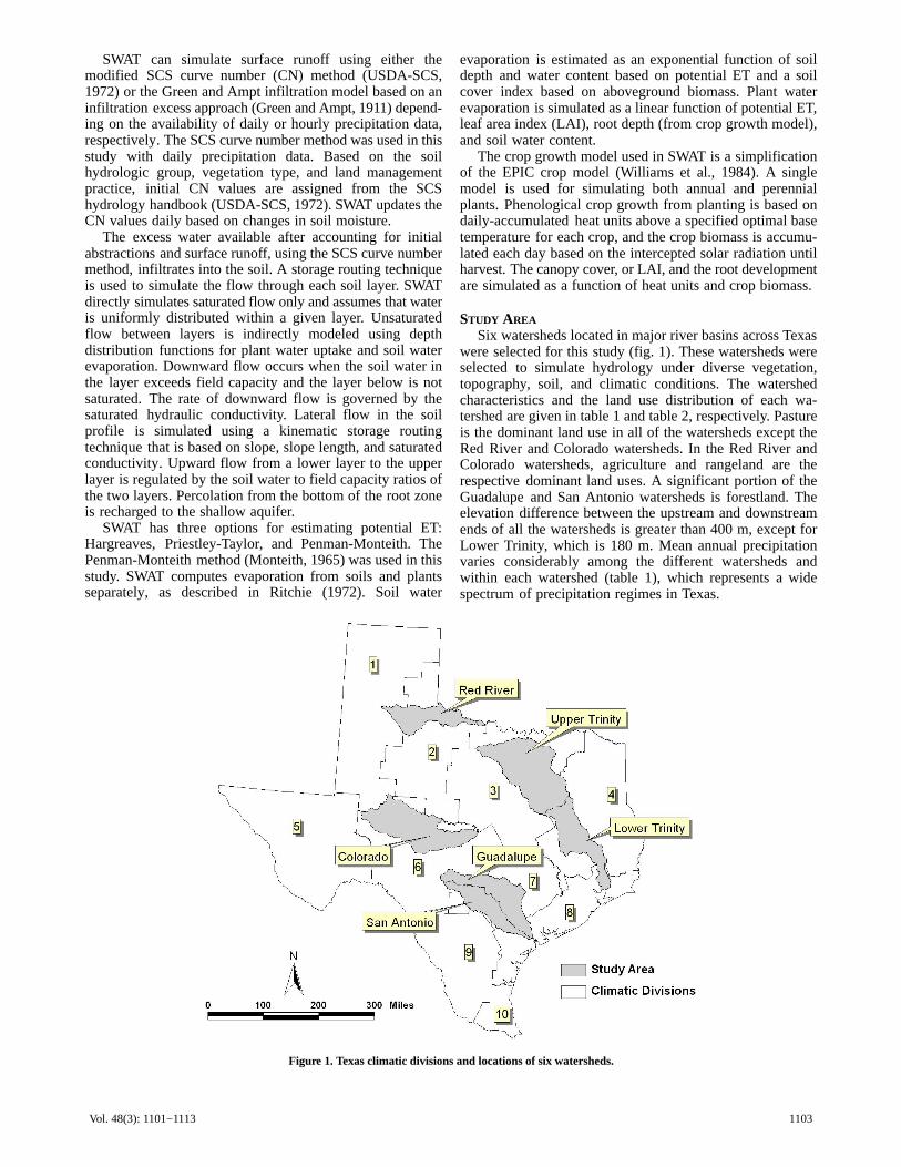
Six watersheds located in major river basins across Texaswere selected for this study (fig. 1). These watersheds wereselected to simulate hydrology under diverse vegetation,topography, soil, and climatic conditions. The watershedcharacteristics and the land use distribution of each wa-tershed are given in table 1 and table 2, respectively. Pastureis the dominant land use in all of the watersheds except theRed River and Colorado watersheds. In the Red River andColorado watersheds, agriculture and rangeland are therespective dominant land uses. A significant portion of theGuadalupe and San Antonio watersheds is forestland. Theelevation difference between the upstream and downstreamends of all the watersheds is greater than 400 m, except forLower Trinity, which is 180 m. Mean annual precipitationvaries considerably among the different watersheds andwithin each watershed (table 1), which represents a widespectrum of precipitation regimes in Texas.

Figure 1. Texas climatic divisions and locations of six watersheds.

1104 TRANSACTIONS OF THE ASAE

Table 1. Watershed characteristics.

Watershed

USGS 6-digitHydrologic Cataloging

Unit NumberArea(km2)

Number of4 × 4 km

Sub-basinsElevation[a]

(m)

Mean AnnualPrecipitation[b]

(mm)

Upper Trinity 120301 29664 1854 78 - 408 729 - 1084Lower Trinity 120302 15200 950 0 - 180 978 - 1368

Red River 111301 11632 727 295 - 1064 488 - 748Guadalupe 121002 14736 921 6 - 728 712 - 990

San Antonio 121003 10320 645 7 - 688 693 - 976Colorado 120901 25656 1541 400 - 886 365 - 708

[a] USGS 7.5 min DEM (USGS, 1993).[b] NRCS PRISM annual precipitation data (Daly et al., 1994).

Table 2. Land use distribution in watersheds obtained from the USGS 1992 National Land Cover Data (NLCD, 1992).

Land Use (%)

Watershed Agriculture Urban Forest Pasture Rangeland Wetland Water

Upper Trinity 5.1 8.8 1.6 79.9 0 0.4 4.2Lower Trinity 1.5 0.8 34.2 54.2 0 6.2 3.1

Red River 49.9 0.1 0 34 16 0 0Guadalupe 1.8 1.1 30.4 59.1 6.2 1.1 0.3

San Antonio 4.3 8.5 32.9 47 6.4 0.6 0.3Colorado 10.3 0.5 1.1 4.9 82.9 0 0.3

MODEL INPUTSWeather inputs needed by SWAT are precipitation,

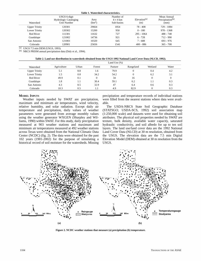
maximum and minimum air temperatures, wind velocity,relative humidity, and solar radiation. Except daily airtemperature and precipitation, daily values of weatherparameters were generated from average monthly valuesusing the weather generator WXGEN (Sharpley and Wil-liams, 1990) within SWAT. For this study, daily precipitationmeasured at 903 weather stations and maximum andminimum air temperatures measured at 492 weather stationsacross Texas were obtained from the National Climatic DataCenter (NCDC) (fig. 2). The data were obtained for the past102 years (1901-2002) for the purpose of simulating ahistorical record of soil moisture for the watersheds. Missing

precipitation and temperature records of individual stationswere filled from the nearest stations where data were avail-able.

The USDA-NRCS State Soil Geographic Database(STATSGO; USDA-SCS, 1992) soil association map(1:250,000 scale) and datasets were used for obtaining soilattributes. The physical soil properties needed by SWAT aretexture, bulk density, available water capacity, saturatedhydraulic conductivity, and soil albedo for up to ten soillayers. The land use/land cover data are the 1992 NationalLand Cover Data (NLCD) at 30 m resolution, obtained fromthe USGS. The elevation data are the 7.5 min DigitalElevation Model (DEM) obtained at 30 m resolution from theUSGS.

(a) (b)

TemperaturegaugeStudyarea

Figure 2. NCDC weather stations that measure (a) precipitation (b) temperature.

1105Vol. 48(3): 1101−1113

MODEL SETUPFor this study, a spatial resolution of 4 × 4 km was chosen

to capture adequate spatial variability over a large watershedand for future integration studies with NEXRAD radarprecipitation that has a similar spatial resolution. TheArcView interface for the model (Di Luzio et al., 2002b) wasused to extract model parameters from the GIS layers withminor modifications to delineate sub-basins at 4 × 4 kmresolution. Each watershed was divided into several sub-ba-sins (grids) at 4 × 4 km resolution, using a DEM resampledto the same resolution (e.g., Upper Trinity was divided into1854 sub-basins, each 4 × 4 km). Topographic parametersand stream channel parameters were estimated from theDEM. A dominant soil and land use type within eachsub-basin was used to develop soil and plant inputs to themodel. Initial curve number values were assigned based onthe soil hydrologic group and vegetation type for an averageantecedent moisture condition (USDA-SCS, 1972). Based onthe land use assigned for each grid, plant growth parameterslike maximum leaf area index, maximum rooting depth,maximum canopy height, and optimum and base tempera-tures, were obtained from a crop database within SWAT. Cornwas assumed to be the crop grown in all agricultural land. Theplanting and harvest dates of crops and active growing periodof perennials were scheduled using a heat unit schedulingalgorithm (Arnold et al., 1998). The weather data for eachsub-basin was assigned from the closest weather station. Inorder to simulate the natural hydrology and long-term soilmoisture balance, all the crops in the watershed wereassumed to be rainfed, and hence irrigation was notconsidered in this study.

CALIBRATION AND VALIDATION OF STREAM FLOW

Stream flow, measured at 24 USGS stream gauges locatedin six watersheds, was used for calibrating and validating themodel. Only those stream gauges that are not affected byreservoirs, diversions, or return flows were selected formodel calibration and validation. Five years of measuredstream flow data were used for model calibration. Thecalibration period for each USGS station was selected aftercareful analysis of the stream flow time series. The fivecontiguous years of stream flow that had fair distribution ofhigh and low flows were selected for model calibration. Thiswas done to obtain optimal parameters that improve themodel simulation in both wet and dry years.

The model was calibrated using the VAO5A Harwelllibrary subroutine (Harwell, 1974), a non-linear auto-calibra-tion algorithm. VAO5A uses a non-linear estimation tech-

nique known as the Gauss-Marquardt-Levenberg method toestimate optimal model parameters. The objective functionis to minimize the mean squared error in the measured versussimulated stream flow. The strength of this method lies in thefact that it can generally estimate parameters using fewermodel runs than other estimation methods (Demarée, 1982).The model parameters selected for auto-calibration using theVAO5A algorithm are listed in table 3. These modelparameters were selected because of the sensitivity of surfacerunoff to them, as reported in several studies (Arnold et al.,2000; Lenhart et al., 2002; Santhi et al., 2001; TexasAgricultural Experiment Station, 2000). In order to preventthe algorithm from choosing extreme parameter values, themodel parameters were allowed to change only withinreasonable limits (table 3).

After optimal calibration of parameters was achieved, themodel was validated at each of the 24 USGS calibrationstations using 10 to 30 years of observed stream flow data,based on data availability. As the objective of this study wasto develop the soil moisture data on a weekly time step, themeasured and simulated stream flow was also averaged overa weekly period for statistical comparison. The coefficient ofdetermination (R2 ) and the coefficient of efficiency (E)(Nash and Sutcliffe, 1970) were the statistics used to evaluatethe calibration and validation results. The R2 and E values arecalculated as follows:

( )( )

( ) ( )

2

1

2

1

2

12R

−−

−−=

∑∑

∑

==

=

N

ii

N

ii

N

iii

PPOO

PPOO��� ���

��� ���

(1)

( )

( )∑

∑

=

=

−

−−=

N

ii

N

iii

OO

PO

1

2

2

10.1E���

(2)

whereOi = observed stream flow at time iPi = predicted stream flow at time i

O���

= mean of the observed stream flow

P���

= mean of the predicted stream flowN = number of observed/simulated values.

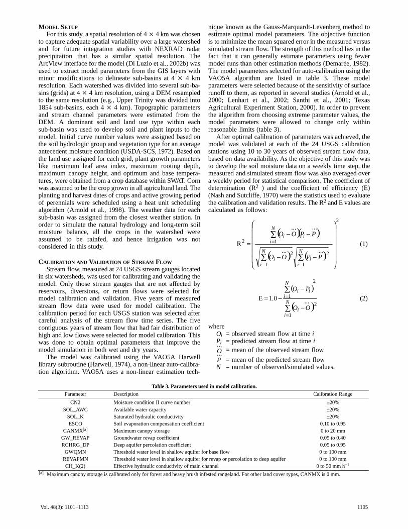
Table 3. Parameters used in model calibration.Parameter Description Calibration Range

CN2 Moisture condition II curve number ±20%SOL_AWC Available water capacity ±20%

SOL_K Saturated hydraulic conductivity ±20%ESCO Soil evaporation compensation coefficient 0.10 to 0.95

CANMX[a] Maximum canopy storage 0 to 20 mmGW_REVAP Groundwater revap coefficient 0.05 to 0.40RCHRG_DP Deep aquifer percolation coefficient 0.05 to 0.95

GWQMN Threshold water level in shallow aquifer for base flow 0 to 100 mmREVAPMN Threshold water level in shallow aquifer for revap or percolation to deep aquifer 0 to 100 mmCH_K(2) Effective hydraulic conductivity of main channel 0 to 50 mm h−1

[a] Maximum canopy storage is calibrated only for forest and heavy brush infested rangeland. For other land cover types, CANMX is 0 mm.

1106 TRANSACTIONS OF THE ASAE

The value of R2 ranges from 0 to 1, with higher valuesindicating better agreement between predicted and observedstream flow. The value of E ranges from −∞ to 1, with Evalues greater than zero indicating that the model is a goodpredictor. R2 evaluates only linear relationships betweenvariables; thus, it is insensitive to additive and proportionaldifferences between model simulations and observations(Willmott, 1984). However, E is sensitive to differences inthe means and variances of observed and simulated data andhence is a better measure to evaluate model simulations(Legates and McCabe, 1999).

SOIL MOISTURE AND VEGETATION INDEX

Stream flow is often the only component of the waterbalance that is regionally observed and, hence, widely usedfor calibrating hydrologic models. However, stream flowaccounts for a smaller fraction of the hydrologic componentthan ET and soil moisture. In the current study, soil water isthe hydrologic component of interest, and it would be idealto use soil moisture and/or ET for calibration if the measureddata were available at the study area in a natural hydrologicsetting (without irrigation). Due to a lack of measured soilmoisture and ET data, a pseudo indicator of soil moisturecondition, the normalized difference vegetation index(NDVI), was used to analyze the model’s predicted soilmoisture.

NDVI is a vegetation index obtained from red and infraredreflectance measured by satellite. It is an indicator of

photosynthetic activity, greenness, and health of vegetation(DeFries et al., 1995). Among various stress factors that af-fect vegetation, water stress is an important factor that affectsphotosynthetic activity and greenness of the vegetation. Far-rar et al. (1994) found that NDVI and soil moisture are wellcorrelated in the concurrent month of the growing season.Hence, NDVI can be a useful indicator to analyze the simu-lated soil moisture during the active growing season of thecrop and to determine the usefulness of soil moisture fordrought monitoring.

Ten-day NDVI composite data measured by NOAA-AVHRR satellite from 1982 to 1998 at a spatial resolution of8 × 8 km was used for this study. The satellite data wasresampled to 4 × 4 km to match the sub-basin resolution usedin this study and was linearly interpolated between two10-day composites to get weekly NDVI data. The weeklyNDVI data were correlated with weekly simulated soilmoisture to evaluate the soil moisture predictions of thehydrologic model.

RESULTS AND DISCUSSIONCALIBRATION AND VALIDATION OF STREAM FLOW

The model was calibrated using the non-linear auto-cal-ibration algorithm VAO5A (Harwell, 1974), and selectedmodel parameters were changed within reasonable limits, asindicated in table 3. The model was calibrated using five

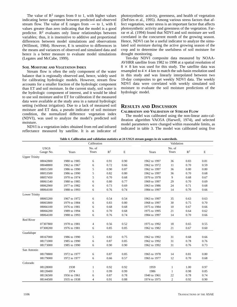
Table 4. Calibration and validation statistics at 24 USGS stream gauges in six watersheds.Calibration Validation

USGSGauge No. Years

No. ofYears R2 E Years

No. ofYears R2 E

Upper Trinity08042800 1980 to 1985 6 0.91 0.90 1962 to 1997 36 0.83 0.8108048800 1962 to 1967 6 0.72 0.66 1962 to 1972 11 0.70 0.5908051500 1986 to 1990 5 0.90 0.87 1962 to 1997 36 0.80 0.8008053500 1986 to 1990 5 0.82 0.80 1962 to 1997 36 0.70 0.6808057450 1970 to 1974 5 0.70 0.68 1970 to 1978 9 0.68 0.6708061540 1980 to 1985 6 0.80 0.77 1969 to 1997 29 0.70 0.6908062900 1977 to 1982 6 0.73 0.69 1963 to 1986 24 0.71 0.6808064100 1988 to 1993 6 0.76 0.74 1984 to 1997 14 0.70 0.66

Lower Trinity08065200 1967 to 1972 6 0.54 0.54 1963 to 1997 35 0.63 0.6308065800 1979 to 1984 6 0.83 0.80 1968 to 1997 30 0.75 0.7008066100 1976 to 1981 6 0.68 0.68 1975 to 1984 10 0.67 0.6608066200 1989 to 1994 6 0.70 0.68 1975 to 1995 21 0.64 0.6208064100 1988 to 1993 6 0.76 0.74 1984 to 1997 14 0.70 0.66

Red River07307800 1978 to 1981 4 0.56 0.52 1975 to 1992 18 0.65 0.5507308200 1976 to 1981 6 0.85 0.85 1962 to 1982 21 0.67 0.60

Guadalupe08167000 1986 to 1990 5 0.82 0.75 1962 to 1992 31 0.68 0.6608171000 1985 to 1990 6 0.87 0.85 1962 to 1992 31 0.78 0.7608173000 1985 to 1990 6 0.90 0.90 1962 to 1992 31 0.76 0.73

San Antonio08178800 1972 to 1977 6 0.87 0.85 1965 to 1978 14 0.81 0.8008179000 1972 to 1977 6 0.66 0.57 1965 to 1977 12 0.70 0.68

Colorado08128000 1938 1 0.92 0.92 1959 1 1.00 0.9708128400 1974 1 0.99 0.99 1986 1 0.98 0.8508136500 1956 to 1961 6 0.87 0.78 1940 to 1961 22 0.78 0.7408144500 1935 to 1938 4 0.91 0.88 1974 to 1975 2 0.92 0.90

1107Vol. 48(3): 1101−1113

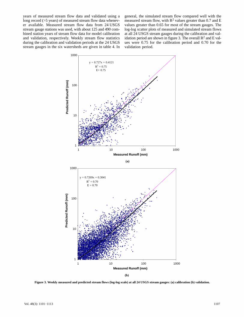
years of measured stream flow data and validated using along record (>5 years) of measured stream flow data whenev-er available. Measured stream flow data from 24 USGSstream gauge stations was used, with about 125 and 490 com-bined station years of stream flow data for model calibrationand validation, respectively. Weekly stream flow statisticsduring the calibration and validation periods at the 24 USGSstream gauges in the six watersheds are given in table 4. In

general, the simulated stream flow compared well with themeasured stream flow, with R2 values greater than 0.7 and Evalues greater than 0.65 for most of the stream gauges. Thelog-log scatter plots of measured and simulated stream flowsat all 24 USGS stream gauges during the calibration and val-idation period are shown in figure 3. The overall R2 and E val-ues were 0.75 for the calibration period and 0.70 for thevalidation period.

y = 0.727x + 0.4121

R2 = 0.75E= 0.75

1

10

100

1000

1 10 100 1000

Measured Runoff (mm)

Pre

dic

ted

Ru

no

ff (m

m)

(a)

y = 0.7269x + 0.3041

R2 = 0.70E = 0.70

1

10

100

1000

1 10 100 1000

Measured Runoff (mm)

Pre

dic

ted

Ru

no

ff (m

m)

(b)

Figure 3. Weekly measured and predicted stream flows (log-log scale) at all 24 USGS stream gauges: (a) calibration (b) validation.

1108 TRANSACTIONS OF THE ASAE

Analysis of time series plots for individual stream gaugesshowed that most of the differences between the observed andmeasured rainfall/stream flow data occurred due to non-availability of a rain gauge at the watershed or precipitationevents that were not measured by a rain gauge nearest to thewatershed. A few runoff peaks observed in each of the 24USGS stream gauges either did not match with the measuredprecipitation data to the same intensity or the precipitation

event was not at all captured by the rain gauge at or near thewatershed. These missed precipitation events resulted inreduced R2 and E statistics at a few USGS stream gauges.Using spatially distributed rainfall from NEXRAD radarcould improve the model results. Overall, the model was wellcalibrated (R2 = 0.75 and E = 0.7), and the simulated streamflow compared well with the observed stream flow undervarying land use, hydrologic, and climatic conditions.

Figure 4. Ratio of growing season ET to growing season precipitation at the six watersheds (AGRL = agriculture, PAST = pasture, RNGE = rangeland,FRSE = evergreen = forest, FRSD = deciduous forest, and FRST - mixed forest).

1109Vol. 48(3): 1101−1113

EVAPOTRANSPIRATIONAnalysis of the simulation results at each watershed

showed that actual growing season ET (March throughOctober) was about 45% to 90% of growing seasonprecipitation (P) and varied with land use and the climaticzone of each watershed. The distributions of ET/P ratioamong each land use for the six watersheds are shown usingbox-and-whisker plots in figure 4. Upper Trinity and LowerTrinity had low ET/P ratios compared to the other watershedsdue to a high amount of precipitation in these watersheds.Red River had the highest ET/P ratio, with over 90% ofprecipitation returning as ET for all the land use classes in thewatershed. Irrespective of the watershed, agriculture andpastureland had the highest ET/P ratio, with 70% to 90% ofprecipitation returning to the atmosphere as ET. This wasbecause agriculture and pastureland were mainly located insoils with high available water capacity. Thus, more waterwas stored from precipitation and was available for ET whencompared to soils of low water holding capacity. Dugas et al.(1999) measured ET by the Bowen ratio/energy balancemethod for Bermuda grass, native prairie, and sorghum at theBlackland Research Center in Temple, Texas, which has anaverage annual precipitation of about 880 mm. The measuredET reported by Dugas et al. (1999) during the growing season(March through October of 1993 and 1994) accounted forabout 75% to 90% of the growing season precipitation. Thismatches well with the model results and indicates that themodel was able to simulate the growing season ET of pastureand agriculture land within reasonable limits.

ANALYSIS OF SIMULATED SOIL WATER USING NDVIStream flow was the only water balance component that

was widely available for the model calibration and valida-tion. The ability of the model to simulate soil water could notbe evaluated quantitatively due to a lack of measured data.Hence, simulated soil water was analyzed using NDVImeasured by NOAA-AVHRR satellite. The weekly NDVIwas compared with simulated average weekly soil water foreach sub-basin during the active phase of the growing season(April to September) from 1982 to 1998 (except 1994). A laganalysis was performed with the current week’s NDVI andthe simulated soil water in the concurrent week and past fourweeks. The lag analysis showed that NDVI lags behindsimulated soil water by at least one week for most of thesub-basins. This was expected because it takes some time forthe plants to respond to the water stress in the root zone.However, the lag between NDVI and soil water was not aconstant and varied from year to year for the same land useand sub-basin. This could be due to the difference in the onsetof seasonal precipitation from year to year and the quantityof precipitation. Nevertheless, for most of the sub-basins, thecorrelation between NDVI and soil water at zero lag was onlyslightly less than the maximum correlation obtained at acertain lag. The distributions of maximum correlationobtained from lag analysis between NDVI and soil wateramong each land use within a watershed is given as abox-and-whisker plot in figure 5. Except for Lower Trinity,in general, there is a good correlation between NDVI andsimulated soil water for agriculture and pastureland covertypes (r ~ 0.6).

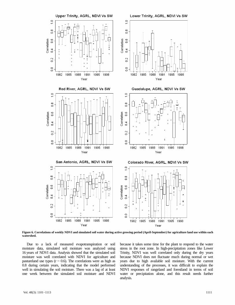
The distributions of correlations between NDVI and soilwater for agricultural sub-basins for each year at sixwatersheds are shown as box-and-whisker plots in figure 6.

The correlations were as high as 0.8 during some years, yetlow in other years. In general, Upper Trinity had bettercorrelation between NDVI and soil water than the otherwatersheds. This is because there is less irrigation activity inthis watershed and the crop growth depends mostly on soilwater replenished by rainfall. In contrast, a large portion ofagricultural lands in the Red River and Colorado Riverwatersheds are under irrigation. Some agricultural lands inRed River grow winter wheat that has a different growingseason than corn. It is a common agricultural practice to growcorn and wheat during alternate years in the same agriculturalfield. Hence, there was a wide distribution of correlation inthe Red River watershed when compared to other wa-tersheds. The lower correlation between NDVI and soil waterfor agricultural lands during certain years could be due toseveral reasons. For example, in Upper Trinity, the lowercorrelations during 1989 and 1992 were because of highprecipitation during those years for which the NDVI responsewas much different from that of other years. Similarly, during1996, much less precipitation was received during thegrowing season. Hence, the NDVI was much less, indicatingno crop growth during that year. This was the same case fora lower correlation at the Guadalupe River watershed during1996 and at the Colorado watershed during 1988 and 1989.In Lower Trinity, there were only a few agricultural lands andthey were scattered adjacent to the wetlands close to Gulf ofMexico. These agricultural lands predominantly grow rice.Further, among the six study areas, Lower Trinity is locatedin a high rainfall zone. Because of the high annual rainfall,the NDVI did not fluctuate much with changes in soil water.Thus, the correlation between NDVI and SW was low atLower Trinity.

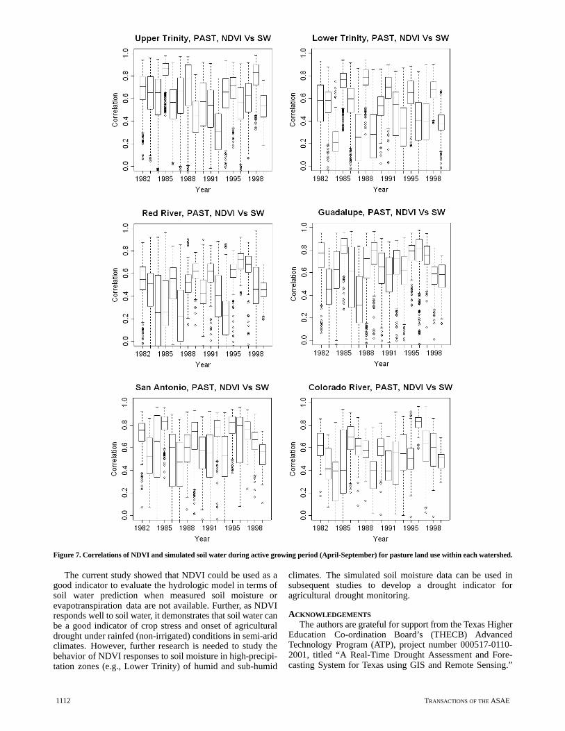
The distributions of correlations between NDVI and soilwater for pasture sub-basins for each year at six watershedsare shown as box-and-whisker plots in figure 7. In general,pasture had a wider spread of correlation distribution acrosssub-basins than agriculture. This could be because pasture iscut and grazed all summer during the growing season.Cutting and grazing of pasture could change the NDVI valuessensed by satellite due to lesser leaf area. Hence, the NDVIfluxes were not purely due to natural soil moisture fluctua-tions alone. The correlation was generally less at LowerTrinity, except during some years. Analysis of precipitationdata showed that the correlation between NDVI and soilwater was markedly high at Lower Trinity during the dryyears 1985 and 1988. This could be because Lower Trinity iswet during most parts of the year, with an annual precipitationof more than 1000 mm, and has a lesser evaporative fractionfor all land use types when compared to the other watersheds(fig. 4). Hence, the fluctuations in soil moisture duringnormal or high precipitation years do not seem to affect theNDVI much, except during dry years when the available soilmoisture becomes less at the root zone.

The NDVI responded well to changes in soil water foragriculture and pasturelands because they have shallow rootsystems that can extract water only from the root zone.However, the NDVI for brush species in rangeland and treesof forestland did not respond well to the simulated soil water.Hence, a lagged correlation analysis was conducted withcurrent NDVI and cumulative precipitation of the past four,eight, and twelve weeks. The analysis (the results are notpresented here) yielded similar or lesser correlations than thatof soil water. Thus, with the current understanding of the

1110 TRANSACTIONS OF THE ASAE

Figure 5. Correlations of weekly NDVI and simulated soil water during active growing period (April-September) of 1982-1998 for all sub-basins withineach watershed (AGRL = agriculture, PAST = pasture, RNGE = rangeland, FRSE = evergreen forest, FRSD = deciduous forest, and FRST = mixedforest).

processes, it was difficult to explain the NDVI responses ofrangeland and forestland in terms of soil water or precipita-tion alone, and this result needs further analysis.

SUMMARY AND CONCLUSIONSThe hydrologic model SWAT was used for developing a

long-term soil moisture dataset at a spatial resolution of 4 ×4 km and at a weekly temporal resolution. The hydrologicmodel was calibrated for stream flow using an auto-calibra-

tion algorithm and validated over multiple years. The overallR2 and E values on weekly stream flow were 0.75 for thecalibration period and 0.70 for the validation period. Most ofthe differences between the measured and simulated streamflow occurred due to the lack of a rain gauge network in thewatershed. This could be overcome by using spatiallydistributed RADAR rainfall data. Overall, the model waswell calibrated, and the simulated stream flow compared wellwith the observed stream flow under varying land use,hydrologic, and climatic conditions.

1111Vol. 48(3): 1101−1113

Figure 6. Correlations of weekly NDVI and simulated soil water during active growing period (April-September) for agriculture land use within eachwatershed.

Due to a lack of measured evapotranspiration or soilmoisture data, simulated soil moisture was analyzed using16 years of NDVI data. Analysis showed that the simulated soilmoisture was well correlated with NDVI for agriculture andpastureland use types (r ~ 0.6). The correlations were as high as0.8 during certain years, indicating that the model performedwell in simulating the soil moisture. There was a lag of at leastone week between the simulated soil moisture and NDVI

because it takes some time for the plant to respond to the waterstress in the root zone. In high-precipitation zones like LowerTrinity, NDVI was well correlated only during the dry yearsbecause NDVI does not fluctuate much during normal or wetyears due to high available soil moisture. With the currentunderstanding of the processes, it was difficult to explain theNDVI responses of rangeland and forestland in terms of soilwater or precipitation alone, and this result needs furtheranalysis.

1112 TRANSACTIONS OF THE ASAE

Figure 7. Correlations of NDVI and simulated soil water during active growing period (April-September) for pasture land use within each watershed.

The current study showed that NDVI could be used as agood indicator to evaluate the hydrologic model in terms ofsoil water prediction when measured soil moisture orevapotranspiration data are not available. Further, as NDVIresponds well to soil water, it demonstrates that soil water canbe a good indicator of crop stress and onset of agriculturaldrought under rainfed (non-irrigated) conditions in semi-aridclimates. However, further research is needed to study thebehavior of NDVI responses to soil moisture in high-precipi-tation zones (e.g., Lower Trinity) of humid and sub-humid

climates. The simulated soil moisture data can be used insubsequent studies to develop a drought indicator foragricultural drought monitoring.

ACKNOWLEDGEMENTS

The authors are grateful for support from the Texas HigherEducation Co-ordination Board’s (THECB) AdvancedTechnology Program (ATP), project number 000517-0110-2001, titled “A Real-Time Drought Assessment and Fore-casting System for Texas using GIS and Remote Sensing.”

1113Vol. 48(3): 1101−1113

The research effort was also partly funded by the Texas WaterResources Institute (TWRI) and Texas Forest Service (TFS).

REFERENCESAkinremi, O. O., and S. M. McGinn. 1996. Evaluation of the palmer

drought index on the Canadian Prairies. J. Climate 9(5): 897-905.Akinremi, O. O., S. M. McGinn, and A. G. Barr. 1996. Simulation of

soil moisture and other components of the hydrological cycle usinga water budget approach. Canadian J. Soil Sci. 76(2): 133-142.

Arnold, J. G., R. Srinivasan, R. S. Muttiah, and J. R. Williams. 1998.Large-area hydrologic modeling and assessment: Part 1. Modeldevelopment. J. American Water Res. Assoc. 34(1): 73-89.

Arnold, J. G., R. S. Muttiah, R. Srinivasan, and P. M. Allen. 2000.Regional estimation of base flow and groundwater recharge in theUpper Mississippi River basin. J. Hydrology 227(1-4): 21-40.

Daly, C., R. P. Neilson, and D. L. Phillips, 1994: Astatistical-topographic model for mapping climatologicalprecipitation over mountainous terrain. J. Applied Meteorology33(2): 140-158.

DeFries, R., M. Hansen, and J. Townsheld. 1995. Global discriminationof land cover types from metrics derived from AVHRR pathfinderdata. Remote Sensing of Environ. 54(3): 209-222.

Demarée, G. 1982. Comparison of techniques for the optimization ofconceptual hydrological models. Mathematics and Computers inSimulation 24(2): 122-130.

Di Luzio, M., R. Srinivasan, and J. G. Arnold. 2002a. Integration ofwatershed tools and SWAT model into basins. J. American WaterRes. Assoc. 38(4): 1127-1141.

Di Luzio, M., R. Srinivasan, J. G. Arnold, and S. L. Neitsch. 2002b.Soil and water assessment tool. ArcView GIS interface manual:Version 2000. TWRI TR-193, College Station, Texas: Texas WaterResources Institute.

Dugas, W. A., M. L. Heuer, and H. S. Mayeux. 1999. Carbon dioxidefluxes over Bermuda grass, native prairie, and sorghum. Agric. andForest Meteorology 93(2): 121-139.

Eckhardt, K., and J. G. Arnold. 2001. Automatic calibration of adistributed catchment model. J. Hydrology 251(1-2): 103-109.

Engman, E. T. 1991. Applications of microwave remote sensing of soilmoisture for water resources and agriculture. Remote Sensing ofEnviron. 35(2-3): 213-226.

Farrar, T. J., S. E. Nicholson, and A. R. Lare. 1994. The influence ofsoil type on the relationships between NDVI, rainfall, and soilmoisture in semiarid Botswana: II. NDVI response to soil moisture.Remote Sensing of Environ. 50(2): 121-133.

Green, W. H., and G. A. Ampt. 1911. Studies on soil physics 1: Theflow of air and water through soils. J. Agric. Sci. 4(1): 1-24.

Hane, D. C., and F. V. Pumphrey. 1984. Crop water use curves forirrigation scheduling. Corvallis, Ore.: Oregon State University,Agricultural Experiment Station.

Harwell. 1974. Harwell library subroutine VAO5A (FORTRANcomputer program). Oxon, U.K.: Hyprotech UK Ltd.

Huang, J., H. M. Van Den Dool, and K. P. Georgakakos. 1996.Analysis of model-calculated soil moisture over the United States(1931-1993) and applications to long-range temperature forecasts. J.Climate 9(6): 1350-1362.

Jackson, T. J., J. Schmugge, and E. T. Engman. 1996. Remote sensingapplication in hydrology: Soil moisture. J. Hydrologic Sci. 41(4):517-530.

Keyantash, J., and J. A. Dracup. 2002. The quantification of drought:An evaluation of drought indices. Bulletin of the AmericanMeteorological Soc. 83(8): 1176-1180.

Legates, D. R., and G. J. McCabe Jr. 1999. Evaluating the use of“goodness-of-fit” measures in hydrologic and hydroclimatic modelvalidation. Water Resources Research 35(1): 233-241.

Lenhart, T., K. Eckhardt, N. Fohrer, and H. G. Frede. 2002.Comparison of two different approaches of sensitivity analysis.Physics and Chemistry of the Earth 27(9-10): 645-654.

Monteith, J. L. 1965. Evaporation and environment. In State andMovement of Water in Living Organisms: Proc. 19th Symposia ofthe Society of Experimental Biology, 205-234. Cambridge, U.K.:Cambridge University Press.

Narasimhan, B. 2004. Development of indices for agricultural droughtmonitoring using a spatially distributed hydrologic model. PhDdiss. College Station, Texas: Texas A&M University.

Nash, J. E., and J. V. Sutcliffe. 1970. River flow forecasting throughconceptual models: Part I. A discussion of principles. J. Hydrology10(3): 282-290.

Neitsch, S. L., J. G. Arnold, J. R. Kiniry, J. R. Williams, and K. W.King. 2002. Soil and water assessment tool. Theoreticaldocumentation: Version 2000. TWRI TR-191. College Station,Texas: Texas Water Resources Institute.

NLCD. 1992. National land cover characterization. Washington, D.C.:U.S. Geological Survey. Available at:http://landcover.usgs.gov/natllandcover.asp. Accessed 15 March2005.

Palmer, W. C. 1965. Meteorological drought. Research Paper No. 45.Washington, D.C.: U.S. Department of Commerce, WeatherBureau.

Ritchie, J. T. 1972. A model for predicting evaporation from a rowcrop with incomplete cover. Water Resources Research 8(5):1204-1213.

Santhi, C., J. G. Arnold, J. R. Williams, W. A. Dugas, R. Srinivasan,and L. M. Hauck. 2001. Validation of the SWAT model on a largeriver basin with point and non-point sources. J. American WaterResources Assoc. 37(5): 1169-1188.

Sellers, P. J., Y. Mintz, Y. C. Sud, and A. Dalcher. 1986. A simplebiosphere model (SiB) for use within general circulation models. J.Atmospheric Sci. 43(6): 505-531.

Sharpley, A. N., and J. R. Williams. 1990. EPIC - erosion productivityimpact calculator: 1. Model documentation. Tech. Bulletin 1768.Washington, D.C.: USDA Agriculture Research Service.

Srinivasan, R., J. G. Arnold, and C. A. Jones. 1998a. Hydrologicmodeling of the United States with the soil and water assessmenttool. International J. Water Resources Development 14(3):315?325.

Srinivasan, R., T. S. Ramanarayanan, J. G. Arnold, and S. T. Bednarz.1998b. Large-area hydrologic modeling and assessment: Part II.Model application. J. American Water Resources Assoc. 34(1):91-101.

Texas Agricultural Experiment Station. 2000. Brush management/wateryield feasibility studies for eight watersheds in Texas. TWRITR-182. College Station, Texas: Texas Water Resources Institute.

USDA-SCS. 1972. National Engineering Handbook. Hydrology,Section 4, Chapters 4-10. Washington, D.C.: USDA SoilConservation Service.

USDA-SCS. 1992. States soil geographic database (STATSGO). DataUser’s Guide. No. 1492. Washington, D.C.: USDA SoilConservation Service.

USGS. 1993. Digital elevation model guide. Washington, D.C.: U.S.Geological Survey. Available at:http://edc.usgs.gov/guides/dem.html. Accessed 15 March 2005.

Van Griensven, A., and W. Bauwens. 2001. Integral water qualitymodelling of catchments. Water Sci. and Tech. 43(7): 321-328.

Williams, J. R., C. A. Jones, and P. T. Dyke. 1984. A modelingapproach to determining the relationship between erosion and soilproductivity. Trans. ASAE 27(1): 129-144.

Willmott, C. J. 1984. On the evaluation of model performance inphysical geography. In Spatial Statistics and Model, 443-460. G. L.Gaile and C. J. Willmott, eds. Dordrecht, The Netherlands: D.Reidel Publishing.