state estimation for enhanced monitoring, reliability ......state estimation for enhanced...
TRANSCRIPT
State Estimation for Enhanced Monitoring, Reliability, Restoration
and Control of Smart Distribution Systems
by
Daniel Andrew Haughton
A Dissertation Presented in Partial Fulfillment
of the Requirements for the Degree
Doctor of Philosophy
Approved August 2012 by the
Graduate Supervisory Committee:
Gerald T. Heydt, Chair
Vijay Vittal
Rajapandian Ayyanar
Kory Hedman
ARIZONA STATE UNIVERSITY
December 2012

i
ABSTRACT
The Smart Grid initiative describes the collaborative effort to modernize the
U.S. electric power infrastructure. Modernization efforts incorporate digital data
and information technology to effectuate control, enhance reliability, encourage
small customer sited distributed generation (DG), and better utilize assets. The
Smart Grid environment is envisioned to include distributed generation, flexible
and controllable loads, bidirectional communications using smart meters and oth-
er technologies. Sensory technology may be utilized as a tool that enhances opera-
tion including operation of the distribution system. Addressing this point, a distri-
bution system state estimation algorithm is developed in this thesis.
The state estimation algorithm developed here utilizes distribution system
modeling techniques to calculate a vector of state variables for a given set of
measurements. Measurements include active and reactive power flows, voltage
and current magnitudes, phasor voltages with magnitude and angle information.
The state estimator is envisioned as a tool embedded in distribution substation
computers as part of distribution management systems (DMS); the estimator acts
as a supervisory layer for a number of applications including automation (DA),
energy management, control and switching.
The distribution system state estimator is developed in full three-phase detail,
and the effect of mutual coupling and single-phase laterals and loads on the solu-
tion is calculated. The network model comprises a full three-phase admittance
matrix and a subset of equations that relates measurements to system states. Net-

ii
work equations and variables are represented in rectangular form. Thus a linear
calculation procedure may be employed. When initialized to the vector of meas-
ured quantities and approximated non-metered load values, the calculation proce-
dure is non-iterative.
This dissertation presents background information used to develop the state
estimation algorithm, considerations for distribution system modeling, and the
formulation of the state estimator. Estimator performance for various power sys-
tem test beds is investigated. Sample applications of the estimator to Smart Grid
systems are presented. Applications include monitoring, enabling demand re-
sponse (DR), voltage unbalance mitigation, and enhancing voltage control. Illus-
trations of these applications are shown. Also, examples of enhanced reliability
and restoration using a sensory based automation infrastructure are shown.

iii
DEDICATIONS
This dissertation is dedicated in part to my parents, Milton and Carol Haugh-
ton, who have provided much support, motivation and inspiration throughout my
academic career; in part to Sasharie J. Haughton, whose continued understanding,
patience and encouragement have also been a great motivating force; and to the
memory of Professor Richard G. Farmer who is perhaps one of the kindest, most
genuine and exceptional power engineers I will ever know.

iv
ACKNOWLEDGEMENTS
I must acknowledge Dr. Gerald T. Heydt for his invaluable guidance, insights
and continued encouragement throughout the writing of this dissertation. Thanks
to the members of the committee, Dr. Vijay Vittal, Dr. Raja Ayyanar and Dr.
Kory Hedman for their comments, feedback and time. Thanks also to Dr. Keith
Holbert, for working with me and encouraging my participation in summer re-
search programs for high-school scholars.
Acknowledgment is due to the Power Systems Engineering Research Center
(PSerc), a Generation III Industry / University Cooperative Research Center, un-
der grant NSF EEC-0001880 and EEC-0968993 and the Future Renewable Elec-
tric Energy Distribution and Management Center (FREEDM), an Engineering Re-
search Center under grant NSF EEC-08212121 for mentorship and financial sup-
port. I would also like to acknowledge the IEEE power and energy society (PES)
for their financial support in attending technical society conferences, and provid-
ing an arena for power systems researchers to grow.

v
TABLE OF CONTENTS
............................................................................................. Page
LIST OF TABLES. .......................................................................................... xiii
LIST OF FIGURES ......................................................................................... xvii
NOMENCLATURE. ...................................................................................... xxiv
CHAPTER
1. THE FUTURE ELECTRIC DISTRIBUTION INFRASTRUCTURE ....... 1
1.1 Scope of this dissertation .......................................................... 1
1.2 The Smart Grid initiative .......................................................... 2
1.3 Industry changes and renewable portfolio standards ................. 4
1.4 Impacts of these changes on distribution systems ..................... 5
1.5 Conventional distribution system design and operation ............ 5
Network design .................................................................... 7
Radial operation of conventional distribution systems .......... 7
High r/x ratios ...................................................................... 8
Short run line segments serving distributed and unbalanced
load...................................................................................... 9
Unbalanced loads, laterals and voltage unbalance .............. 10
Low penetration of installed DG ........................................ 12
Voltage regulation ............................................................. 12
Over-current protection ...................................................... 13

vi
CHAPTER .......... Page
Conventional sensors and measurements in distribution
systems .............................................................................. 13
Revenue metering and historical load data ......................... 14
Distribution system modeling and simulation ..................... 14
1.6 The smart distribution system and need for state
estimation............................................................................... 15
High penetration of distributed generation and storage ....... 15
Impact of solar and wind DG intermittency on distribution
circuits ............................................................................... 16
Networked primary and secondary systems ........................ 16
Demand response and increased customer participation ..... 17
Improved modeling of distribution networks ...................... 18
Distribution automation ..................................................... 18
Smart meters and the advanced metering infrastructure ...... 19
Phasor measurements in the power system ......................... 19
Other considerations .......................................................... 20
1.7 Power system state estimation ................................................ 21
1.8 Distribution system state estimation ....................................... 22
1.9 Organization of this dissertation ............................................. 23

vii
CHAPTER .......... Page
2. DISTRIBUTION SYSTEM RELIABILITY AND RESTORATION...... 24
2.1 Distribution system reliability ................................................ 24
2.2 Basic reliability indices .......................................................... 24
2.3 Improving distribution system reliability ................................ 28
2.4 Distribution system restoration ............................................... 29
2.5 A network theoretic approach to distribution system
reliability ................................................................................ 30
2.6 The binary bus connection matrix ........................................... 33
2.7 Application of B matrix to power system reliability and
restoration .............................................................................. 34
2.8 Sensors for reconfiguration and restoration............................. 38
3. A DISTRIBUTION CLASS STATE ESTIMATOR ............................... 41
3.1 State estimation in the distribution system .............................. 41
3.2 Applications of a distribution class estimator .......................... 42
3.3 Synchronized phasor measurements in power system
state estimation....................................................................... 43
3.4 Conventional state estimation formulation .............................. 44
3.5 The gain matrix in power system state estimation ................... 46
3.6 A three-phase, linear distribution system state estimator
using synchronized phasor measurements............................... 48

viii
CHAPTER ......................... Page
3.7 Three-phase radial distribution ladder iterative power
flow ....................................................................................... 50
3.8 Three-phase unbalanced distribution state estimation ............. 53
3.9 Condition number and state estimation ................................... 54
3.10 Assignment of weights to calculated currents ......................... 57
3.11 Bad data detection and the distribution system state
estimator ................................................................................ 60
4. ILLUSTRATIONS OF RELIABILITY ENHANCEMENT IN THE
SMART GRID ....................................................................................... 61
4.1 Reliability and the Smart Grid: test cases for reliability
enhancement and restoration strategies ................................... 61
4.2 The RYG test system.............................................................. 62
4.3 The Roy Billinton test system-RBTS ...................................... 63
4.4 The large scale simulation system (LSSS) test bed ................. 64
4.5 Illustration of Smart Grid planning, restoration and
reconfiguration ....................................................................... 64
4.6 Interrupting device location .................................................... 66
4.7 Reconfiguration and restoration .............................................. 68
4.8 Reliability enhancement and switching automation on
the RBTS ............................................................................... 70
ix
CHAPTER ......................... Page
4.9 Discussion of reliability enhancement and restoration
examples ................................................................................ 74
5. ILLUSTRATIONS OF THREE-PHASE DISTRIBUTION SYSTEM
STATE ESTIMATION .......................................................................... 76
5.1 Distribution system state estimation ....................................... 76
Approximating non-measured load values.......................... 83
Example SE1 ..................................................................... 85
Results of example SE1 ..................................................... 89
Example SE2 ..................................................................... 91
Results of example SE2 ..................................................... 92
Example SE3 ..................................................................... 97
Results of example SE3 ..................................................... 99
5.2 Biased measurements for improved estimation ..................... 102
Results of biased estimation - example SE2 ..................... 103
Results of biased estimation - example SE3 ..................... 103
Discussion of unbiased distribution system state estimation
results .............................................................................. 107
5.3 Illustration of bad data detection........................................... 107
5.4 Discussion of results ............................................................ 107

x
CHAPTER ............................................................................................ Page
Discussion of biased distribution system state estimation
results .............................................................................. 109
Discussion of bad data detection ...................................... 110
6. ILLUSTRATIONS OF APPLICATIONS OF NON-LINEAR, THREE
PHASE DISTRIBUTION SYSTEM STATE ESTIMATOR ................ 111
6.1 Voltage unbalance ................................................................ 111
6.2 Voltage control..................................................................... 111
6.3 Distributed generation .......................................................... 116
Bidirectional flows with DG (Example DG1) ................... 118
Voltage control using an estimator signal to alter DG power
factor (Example DG2)...................................................... 120
Using energy storage and DG to reduce peak demand,
example DG3 ................................................................... 121
6.4 Large Scale Simulation System test bed (LSSS)
illustration ............................................................................ 123
6.5 An application of distribution state estimation for
demand response, energy and power management,
example DR1 ....................................................................... 125
Example DR1 .................................................................. 126
Example DR1 results ....................................................... 127

xi
CHAPTER ............................................................................................ Page
6.6 Discussion of results ............................................................ 132
Discussion of voltage unbalance studies, examples VU1-VU6
........................................................................................ 132
Discussion of DG and storage results, examples DG1-DG3
........................................................................................ 132
Discussion of LSSS illustration example DR1.................. 133
7. CONCLUSIONS, RECOMMENDATIONS AND FUTURE WORK .. 134
7.1 Contributions and concluding remarks ................................. 134
7.2 General recommendations .................................................... 135
7.3 Future work .......................................................................... 138
REFERENCES .............................................................................................. 139
APPENDIX
A. POWER FLOW RESULTS OF DIFFERENT MODELING
ASSUMPTIONS .................................................................................. 154
B. FORWARD / BACKWARD LADDER ITERATIVE POWER FLOW
ALGORITHM ..................................................................................... 159
C. CONDITION NUMBER OF A MATRIX ................................................... 164
D. ASSIGNING WEIGHTS TO CALCULATED CURRENTS....................... 169
E. RYG TEST BED DATA ............................................................................. 173

xii
APPENDIX Page
F. RBTS TEST BED MODELING AND LOAD ASSUMPTIONS ................. 175
G. RBTS FEEDER F1 WITH DISTRIBUTED GENERATION ...................... 180
H. ILLUSTRATIVE EXAMPLES DESCRIBED ............................................ 184
I. SAMPLE MATLAB CODE ......................................................................... 186

xiii
LIST OF TABLES.
Table ............................................................................................................. Page
1.1 Salient Points of Title XIII of the EISA of 2007 ............................................. 2
1.2 Distribution Level Requirements and Impacts of Smart Grid Initiative Items –
Potential Applications Enhanced by Distribution State Estimation ................ 6
1.3 Conventional Transmission and Distribution System Measurements ............ 13
2.1 Sample Optimal Operating Strategies for Restoration .................................. 39
2.2 Quantities Sensed for Distribution System Restoration ................................ 40
4.1 Examples Presented in Chapter 4 ................................................................. 61
4.2 Results of the Breaker Placement Algorithm ................................................ 68
4.3 Seven Cases for RBTS Reliability and Automation Illustrations .................. 70
4.4 Base Case Reliability Indices for Bus 3 of the RBTS System ....................... 74
4.5 Reliability Indices for Bus 3 of the RBTS with Electronic Switching ........... 74
5.1 Examples Presented in Chapter 5 ................................................................. 76
5.2 Description of Distribution State Estimation Illustrations ............................. 79
5.3 RBTS Feeder F1 Loading Conditions Considered for SE Examples ............. 81
5.4 Feeder Load as Seen by the Substation Transformer for Each Case .............. 82
5.5 Demand at Each Bus Used in SE3a, SE3b, and SE2 ..................................... 85
5.6 Bus Voltages from a Power Flow Study for HE7 Loading Condition, Case C1,
RBTS Feeder F1, Figure 5.1 ....................................................................... 88

xiv
Table ............................................................................................................. Page
5.7 Line Currents from Power Flow Study for HE7 Loading Condition, Case C1,
RBTS Feeder F1, Figure 5.1 ....................................................................... 88
5.8 Estimated Bus Voltages, RBTS Feeder F1, Figure 5.1–Case C1 ................... 90
5.9 Bus Voltages from a Power Flow, RBTS Feeder F1, Figure 5.1–HE3, Case C6
................................................................................................................... 93
5.10 Voltages from a Power Flow, RBTS Feeder F1, Figure 5.1, HE18, Case C5
................................................................................................................... 94
5.11 Line Currents from a Power Flow Solution, RBTS Feeder F1, Figure 5.1,
Light Loading (HE3 – Case C6) and Peak Loading (HE18 – Case C5) ....... 94
5.12 Values of Non-Metered (Pseudo-Measurement) Loads Obtained from
Equations (5.2) – (5.7) at HE5 .................................................................... 97
5.13 Bus Voltages from a Power Flow Study, RBTS Feeder F1 for Loading
Condition HE5 ........................................................................................... 98
5.14 Line Currents Obtained from a Power Flow Study, RBTS Feeder F1, Figure
5.1, HE 5 .................................................................................................... 99
5.15 Measurement Type, Standard Deviation and Weights .............................. 103
5.16 Sample Bad Data Detection Results on Example SE2 .............................. 107
5.17 Comparison of Maximum Error Magnitudes for Unbiased and Biased
Estimates of Voltage and Current for SE3a and SE3b ............................... 110
6.1 Bus Voltage Magnitudes and Unbalance for Case C5 ................................. 113

xv
Table ............................................................................................................. Page
6.2 Results of Controlling Voltage Unbalance on RBTS feeder F1, as Shown in
Figure 5.1, with Capacitors and Reactors .................................................. 115
6.3 Examples Illustrating the Presence of DG in Distribution Systems ............. 117
6.4 Specified load on Each Phase for RBTS Feeder F2, Figure 4.3 .................. 124
6.5 Specified load on Each Phase for RBTS Feeder F3, Figure 4.3 .................. 124
6.6 Specified load on Each Phase for RBTS Feeder F4, Figure 4.3 .................. 125
6.7 Specified load on Each Phase for RBTS Feeder F6, Figure 4.3 .................. 125
6.8 Load Curtailed for RBTS Feeder F2, Figure 4.3, Example DR 1 ................ 126
6.9 Load Curtailed for RBTS Feeder F3, Figure 4.3, Example DR 1 ................ 126
6.10 Load Curtailed for RBTS Feeder F4, Figure 4.3, Example DR 1 .............. 127
6.11 Load Curtailed for RBTS Feeder F6, Figure 4.3, Example DR 1 .............. 127
6.12 Ideal and Estimated Post-Curtailment Loads, Feeder F2, Example DR1 .. 129
6.13 Ideal and Estimated Post-Curtailment Loads, Feeder F3, Example DR1 .. 130
6.14 Ideal and Estimated Post-Curtailment Loads, Feeder F4, Example DR1 .. 130
6.15 Ideal and Estimated Post-Curtailment Loads, Feeder F6, Example DR1 .. 131
7.1 Contributions of this research..................................................................... 135
7.2 Discussion and Observations of Illustrations Presented ............................. 137
A.1 Base Case Comparison of Voltage Magnitudes from an Exact and
Approximate Model ................................................................................. 154

xvi
Table ............................................................................................................. Page
A.2 Case C5 Comparison of Voltage Magnitudes from an Exact and Approximate
Model ....................................................................................................... 155
D.1 Real and imaginary expressions for Taylor series expansion of ... 170
D.2 Measurement data used to illustrate approximation of variance ................. 171
D.3 Results for approximate real and imaginary current variance ..................... 171
E.1 Bus Load Data for the RYG Test System ................................................... 173
E.2 Line Data for the RYG Test System ......................................................... 173
F.1 Data for Feeder F1 Load Profile as Seen at the Substation Transformer ..... 177
F.2 Feeder F1 Load Points, Customer Type, Load and Phase ........................... 178
F.3 Conductor impedance data for all voltage classes....................................... 178
F.4 Base Voltages, Impedance and Current ...................................................... 178
G.1 Solar Injection Values (MW) and Net Load for 24 Hour Profile on RBTS
Feeder F1 ................................................................................................. 181
G.2 Wind Injection Values (MW) and Net Load for 24 Hour Profile on RBTS
Feeder F1 ................................................................................................. 182
H.1 Illustrative examples presented throughout this dissertation ...................... 184

xvii
LIST OF FIGURES
Figure ............................................................................................................ Page
1.1 Depiction of the Smart Grid concept .............................................................. 4
1.2 An example of conventional distribution system design ................................. 8
1.3 Typical r/x ratios for distribution and transmission ACSR conductors ............ 9
2.1 Approximating small increments in ASAI changes with Equation (2.6) ....... 26
2.2 System representation of series connected components ................................ 27
2.3 System representation of parallel connected components ............................. 27
2.4 (a) A directed graph; (b) an undirected graph ............................................... 32
2.5 B matrix algorithm to be used in distribution system applications................. 35
2.6 Sensing and real time monitoring of distribution system elements for
computer assisted calculation and control .......................................................... 37
2.7 System status table indicating status of breakers, buses, lines and loads ....... 37
2.8 An automated restoration / reconfiguration algorithm .................................. 39
3.1 Line impedance between buses n and m ...................................................... 52
3.2 Three-phase unbalanced distribution state estimation overview .................... 53
4.1 One line diagram of the RYG distribution system ........................................ 62
4.2 RBTS one-line diagram showing Bus 3 distribution network, recreated from
[38].................................................................................................................... 63
4.3 The Large Scale Simulation System test bed ................................................ 65
4.4 Expectation of unserved energy vs. no. of interruption devices RYG ........... 69

xviii
Figure ............................................................................................................ Page
4.5 Expectation of unserved energy vs. no. of interruption devices RBTS ......... 72
4.6 SAIDI versus number of interruption devices RBTS .................................... 72
5.1 Three-phase detail of RBTS feeder F1 ........................................................ 76
5.2 Graphic of operating points for HE3, HE5, HE7 and HE18. ......................... 80
5.3 Phase A bus voltage magnitudes (a) along the main feeder and (b) at load
buses, cases C1-C6 ............................................................................................ 86
5.4 Phase B bus voltage magnitudes (a) along the main feeder and (b) at load
buses, cases C1-C6 ............................................................................................ 86
5.5 Phase C bus voltage magnitudes (a) along the main feeder and (b) at load
buses, cases C1-C6 ............................................................................................ 86
5.6 Flowchart of the distribution system state estimation algorithm................... 87
5.7 Main feeder bus voltage magnitudes for the power flow (PF) and estimated
(SE) solutions for HE 7 loading condition, Case C1 ........................................... 89
5.8 Bus voltage phase angle error (i.e. difference between power flow and
estimated), for HE 7 loading condition, Case C1 ................................................ 89
5.9 Main feeder line current magnitudes from power flow (PF) and estimated
(SE), for HE7 loading condition, Case C1 .......................................................... 90
5.10 Difference between current magnitudes for the power flow and estimated
solution corresponding to HE 7 loading condition, Case C1 ............................... 91

xix
Figure ............................................................................................................ Page
5.11 Current phase angle error histogram (i.e. difference between power flow and
estimated solution), for HE7 loading condition, Case C1 ................................... 91
5.12 Bus voltage magnitudes along main feeder RBTS feeder F1, Figure 5.1, for
HE18 loading condition, power flow and estimated solution .............................. 93
5.13 Voltage magnitude error histogram (i.e. difference between power flow and
estimated solution), example SE2 ...................................................................... 95
5.14 Bus voltage phase angle error histogram (i.e. difference between power flow
study and estimated), example SE2 .................................................................... 95
5.15 Line current magnitudes along the main feeder for RBTS feeder F1, power
flow and estimated ............................................................................................. 96
5.16 Branch current magnitude error (Amps), RBTS feeder F1, SE2 ................. 96
5.17 Branch current phase angle error (deg.), RBTS feeder F1, SE2 ................. 96
5.18 Bus voltage magnitudes along the main feeder for HE5 loading condition
based on ‘h sto cal data’ from HE3 (SE3a), then from HE7 (SE3b) ................ 100
5.19 Voltage magnitude error histograms (i.e. difference between power flow
study and estimated), examples SE3a, SE3b..................................................... 100
5.20 Voltage phase angle error histograms (i.e. difference between power flow
study and estimated), examples SE3a, SE3b..................................................... 100
5.21 Line current magnitudes along the main feeder for HE5 loading condition
based on ‘h sto cal data’ from HE3 (SE3a), then from HE7 (SE3b) ................ 101

xx
Figure ............................................................................................................ Page
5.22 Line current magnitude error histograms (i.e. difference between power flow
study and estimated), examples SE3a, SE3b..................................................... 101
5.23 Line current phase angle error histograms (i.e. difference between power
flow study and estimated), examples SE3a, SE3b............................................. 101
5.24 Comparison of unbiased versus biased voltage magnitude and angle
estimates for example SE2 ............................................................................... 104
5.25 Comparison of voltage magnitude and phase angle error histograms for
unbiased and biased estimates corresponding to example SE3a ........................ 104
5.26 Comparison of current magnitude and phase angle error histograms for
unbiased and biased estimates corresponding to example SE3a ........................ 105
5.27 Comparison of voltage magnitude and phase angle error histograms for
unbiased and biased estimates corresponding to example SE3b ....................... 106
5.28 Comparison of current magnitude and phase angle error histograms for
unbiased and biased estimates corresponding to example SE3b ....................... 106
6.1 VU 3: Bus voltage magnitudes along the main feeder of RBTS feeder F1,
Figure 5.1, after switching 300 kVAr capacitors into phase A and B only ......... 114
6.2 VU 4: Bus voltage magnitudes along the main feeder of RBTS feeder F1,
Figure 5.1, after switching capacitors into phases A, B, and switching a reactor
into phase C ..................................................................................................... 115

xxi
Figure ............................................................................................................ Page
6.3 VU 5: Bus voltage magnitudes along the main feeder of RBTS feeder F1,
Figure 5.1, after switching in a 300 kVAr reactor on phase C .......................... 116
6.4 VU 6: Bus voltage magnitudes along the main feeder of RBTS feeder F1,
Figure 5.1, after switching 500 kVAr/ph caps into phase A and B, and a 200 kVAr
reactor into phase C ......................................................................................... 116
6.5 One-line diagram, loads and injections for RBTS feeder F1 with DG at HE3
(Example DG1) ............................................................................................... 119
6.6 Bus voltage profile for the loading condition of RBTS feeder F1 shown in
Figure 6.5 (Example DG1) .............................................................................. 120
6.7 Bus voltage profile for the loading condition of RBTS feeder F1 shown in
Figure 6.5 when DG power factor is changed to absorb reactive power, example
DG2 ................................................................................................................ 121
6.8 Energy storage and DG used to reduce peak load seen by the substation
serving the RBTS feeder F1 (Example DG3) ................................................... 122
6.9 Transmission network and bus 3 distribution subtransmission network for the
LSSS test bed where transmission buses are numbered from 101-107, and bus 103
is bus 3 at 138 kV as indicated in Figure 6.7 .................................................... 124
6.10 Bus voltage magnitudes before and after DR at HE18 on main feeder buses
for RBTS feeder F2, example DR1 .................................................................. 128

xxii
Figure ............................................................................................................ Page
6.11 Bus voltage magnitudes before and after DR at HE18 on main feeder buses
for RBTS feeder F3, example DR1 .................................................................. 128
6.12 Bus voltage magnitudes before and after DR at HE18 on main feeder buses
for RBTS feeder F4 ......................................................................................... 129
6.13 Bus voltage magnitudes before and after DR at HE18 on main feeder buses
for RBTS feeder F6 ......................................................................................... 129
6.14 Solving the RBTS transmission network after DR load curtailment .......... 131
A.1 Bus voltage magnitudes at main feeder buses for detailed and approximate
model, Case C2: heavy load 1 .......................................................................... 156
A.2 Bus voltage magnitudes at main feeder buses for detailed and approximate
model, Case C3: heavy load 2 .......................................................................... 156
A.3 Bus voltage magnitudes at main feeder buses for detailed and approximate
model, Case C4: heavy load 2 with shunt capacitor at bus 48 ........................... 156
A.4 Bus voltage magnitudes at main feeder buses for detailed and approximate
model, Case C5: heavy load 3 (peak) ............................................................... 157
A.5 Bus voltage magnitudes at main feeder buses for detailed and approximate
model, Case C6: light load ............................................................................... 157
B.1 Forward sweep algorithm overview 1 of 2 ................................................. 159
B.2 Forward sweep algorithm overview 2 of 2 ................................................. 160
B.3 Backward sweep algorithm overview 1 of 2 .............................................. 161

xxiii
Figure ............................................................................................................ Page
B.4 Backward sweep algorithm overview 2 of 2 .............................................. 162
C.1 Graphic representation of condition number, estimation and solution accuracy
........................................................................................................................ 166
F.1 Load profile seen at the distribution transformer of RBTS Bus 3 feeder F1 176
F.2 Line geometry for RBTS feeder F1 ............................................................ 176
G.1 Load, solar DG injection and net load profiles for a 24 hour peak day as seen
by RBTS feeder F1 .......................................................................................... 180
G.2 Load, wind DG injection and net load profiles for a 24 hour peak day as seen
by RBTS feeder F1 .......................................................................................... 181

xxiv
NOMENCLATURE.
A Adjacency matrix
ACSR Aluminum Conductor Steel Reinforced
AMI Advanced metering infrastructure
ASAI Average service availability index
AWG American Wire Gauge
AWEA American wind energy association
B Binary connection matrix
CAIDI Customer average interruption duration index
CT Current transformer
DER Distributed energy resources
DG Distributed generation
DoE Department of energy
DMS Distribution management system
DR Demand side response
DSM Demand side management
DSSE Distribution system state estimator
e Error vector
E Set of edges; Expectation of unserved energy (kWh/outage or kWh/y)
EISA Energy independence and security act
FDIR Fault detection, isolation and reconfiguration
FREEDM Future renewable electric energy delivery and management

xxv
G Gain matrix in state estimation
GMR Geometric mean radius
GPS Global positioning system
h, h(x) Process matrix in state estimation calculation
h+ Moore-Penrose pseudo-inverse
hLM Line measurement coefficient matrix
hmeas h matrix subset relating measurement to state variables
Imeas Injection current measurement vector (phasor)
Iline Line current measurement (phasor)
IEEE Institute of Electrical and Electronics Engineers
IPP Independent power producer
ISO Independent system operator
IT Information technology
J Incidence matrix
J(x) Objective function of state estimation formulation
LSSS Large Scale Simulation System Test Bed
m Number of circuit breakers that are open
Mi Mean of variable i
MLE Maximum likelihood estimation
n Number of elements in a vector or a row or column designator in a
matrix
N Set of nodes

xxvi
N(0,1) Standard normal distribution, zero mean, unit variance
nb Number of buses
ncb Number of circuit breakers
nl Number of lines
n_ph Number of phases
N9 N9’ Number of nines in reliability
NSF National Science Foundation
OMS Outage management system
p Order of a norm
PCC Point of common coupling
PHEV Plug-in hybrid electric vehicles
PMU Phasor measurement unit
PSERC Power Systems Engineering Research Center
PT Potential transformer
Q Reactive power
r Residual vector in state estimation; repair time; expected outage du-
ration in hours
r/x Ratio of conductor resistance to reactance
R Covariance matrix of measurement weights
RBTS A test bed distribution system ‘Roy Billinton Test System’
RES Renewable energy standard
RPS Renewable portfolio standard

xxvii
RTO Regional transmission organization
RYG A test bed distribution system ‘Red-Yellow-Green’
smax Maximum singular value
smin Minimum singular value
SAIDI System average interruption duration index
SAIFI System average interruption frequency index
SCADA Supervisory control and data acquisition
SST System status table
U Annual unavailability (h/y); the identity matrix
Three-phase voltage vector at bus n
Vmeas Voltage measurement vector (phasor)
Vark The variance of variable k
WLS Weighted least squares
W Weight matrix in state estimation
x Solution vector of a linear system, a state vector
X Reactance
Y, Ybus Bus admittance matrix
z Measurement vector
Zaa Phase a conductor the self impedance in a three-phase network
Zab Mutual impedance between phases a and b in a three-phase network
Three-phase block impedance matrix, with self impedance and mutu-
al impedance

xxviii
Zm Mutual impedance between phases in a three-phase network
ΔASAI Small increment in the ASAI index
ΔSAIDI Small increment in the SAIDI index
ΔT Time interval between measurement samples
δ Bus voltage phase angle
η A measurement noise vector
Ireal Expectation of the real part of the calculated current, I
Iimag Expectation of the imaginary part of the calculated current, I
κ Condition number of a matrix
λ Expected failure rate (failures/y)
σ, σk Standard deviation, standard deviation of measurement k
φ A phase in a three phase system, e.g., φ = a b c
Estimated quantity
(·)H Hermitian operation (complex conjugation followed by transposition)
(·)r, (·)i Real and imaginary parts of a complex quantity
Combinatorial
||· ||p A p-norm of a vector
(·)t Transposition
Boolean OR operation
Boolean AND operation

1
1. The future electric distribution infrastructure
1.1 Scope of this dissertation
A distribution class state estimator is proposed as a feasible response to re-
quirements for enhanced monitoring and control of a power distribution system in
the Smart Grid environment. The Smart Grid initiative in the U.S. and similar ini-
tiatives globally are direct drivers of power grid modernization. Major weakness-
es identified in contemporary distribution system architectures include the lack of
feeder monitoring and visualization technology and a lack of control options.
As envisioned here, the estimator is a tool to facilitate: higher penetrations of
distributed generation (DG); switching; distribution automation (DA); voltage
scheduling; and optimized reactive power injections. Efficient operation, en-
hanced reliability and rapid restoration become possible. The estimator is de-
signed to run in a distribution management system (DMS) supervisory application
that utilizes measurements to calculate feasible solutions to solve near real-time
operational issues, and alert operators to abnormal or problematic conditions.
This dissertation addresses the following as they relate to power distribution
systems: the Smart Grid initiative; implications on future systems; theory of relia-
bility and restoration; sensory based automation; characteristics of conventional
versus smart systems; modeling assumptions used to build estimator algorithms;
measurement infrastructure; historical context of state estimation; and formulation
of a linear, non-iterative, three-phase distribution class state estimator.

2
Notable applications of the state estimation algorithm are illustrated. Applica-
tions include demand response (DR), voltage unbalance minimization, load esti-
mation and enhanced voltage control. This dissertation attempts to analyze and
obviate distribution level impacts of the Smart Grid initiative.
1.2 The Smart Grid initiative
The Smart Grid initiative may be summarized as the modernization of the
U.S. electric energy infrastructure as discussed in the U.S. Department of Energy
(DoE) Grid 2030 vision [1]-[6]. The salient points of Title XIII of the Energy In-
dependence and Security Act (EISA) of 2007 [1] outline plans for a modern, reli-
able and secure electric infrastructure and are discussed in Table 1.1. Figure 1.1
is a graphic depiction of the Smart Grid concept.
Table 1.1 Salient Points of Title XIII of the EISA of 2007
1. Increased use of digital information and controls technology to improve
reliability, security, and efficiency of the electric grid.
2. Dynamic optimization of grid operations, with full cyber-security.
3. Deployment and integration of distributed energy resources (DER) and
distributed generation (DG), including renewable resources.
4. Development and incorporation of demand response (DR), demand-side
management (DSM) resources, and energy-efficiency resources.
5. Deployment of ‘smart’ technologies for metering, communications con-
cerning grid operations and status, and distribution automation.
6. Integration of ‘smart’ appliances and consumer devices.
7. Deployment and integration of advanced electricity storage and peak-
shaving technologies, including plug-in electric and hybrid electric vehi-
cles (PHEV), and thermal-storage air conditioning.
8. Provision to consumers of timely information and control options.
9. Development of standards for communication and interoperability of ap-
pliances and loads, including infrastructure serving the grid.
10. Identification and lowering of unreasonable or unnecessary barriers to
adoption of Smart Grid technologies, practices, and services.

3
This research is part of a Power Systems Engineering Research Center
(PSERC) project entitled “Implications of the Smart Grid Initiative on Distribu-
tion Engineering”. The project statement identifies that ‘Smart Grid initiatives’
and similarly named efforts are targeting the modernization of the electricity grid.
Noticing that efforts have largely focused on transmission system improvements,
the project attempts to identify adaptations of the distribution system. This effort
includes studying selective conversion to networked distribution, utilization of
sensory signals at the local and hierarchically higher levels for both supervised
and fully automated control, and the development of enabling strategies and inter-
connection configurations for renewable resources at the distribution system level.
This work is also supported in part by the National Science Foundation (NSF)
under the Engineering Research Center program in a national ERC denominated
FREEDM (Future Renewable Electric Energy Delivery and Management) center.
The focus of FREEDM is the use of solid state devices for power system control.
The use of solid state controllers considered here relate to the following roles:
Rescheduling of power during restoration
Control of DG – particularly renewable generation resources
Control of selected loads to effectuate peak demand reduction.
Additionally, visualization is a key element of distribution system operation,
and this too is part of the FREEDM portfolio; this is an important focus of state
estimation in distribution systems. References [7], [8] relate to the FREEDM mis-
sion.

4
1.3 Industry changes and renewable portfolio standards
The deregulation and subsequent restructuring in many parts of the U.S. elec-
tric power industry assumes that a market based structure offers greater benefit to
consumers as competing suppliers enter the market; this concept is elaborated in
[9]-[15]. However, distribution businesses generally remain heavily regulated.
Also, environmental concerns manifest themselves in regulations or incentives.
An illustration of this point is the Renewable Portfolio Standard (RPS). RPSs are
present in 34 U.S. states as of September, 2011; note that RPSs encourage renew-
able sources like solar and wind [16]-[18] and may provide penalties for utilities
that fail to meet goals. Also, independent power producers (IPPs) become major
participants in supplying electric power.
Figure 1.1 Depiction of the Smart Grid concept

5
1.4 Impacts of these changes on distribution systems
The impacts of deregulation and renewable incentives on distribution systems
may be seen globally. In territories with aggressive RPS (or goals), small renewa-
ble electric generators are often connected at the distribution level. For example,
California and Ireland target 33% and 40% of energy served must be supplied by
renewables by 2020 [17], [21], [23]. Ireland expects 50% of new wind generators
to be installed at distribution voltage. These events outline significant departure
from conventional utility generation expansion. IPPs and small residential solar
PV and wind farms are necessary to meet aggressive RPS targets.
The power system issues of monitoring, operation and control are likely to ex-
tend into the distribution level. Operators may seek to expand mitigation options
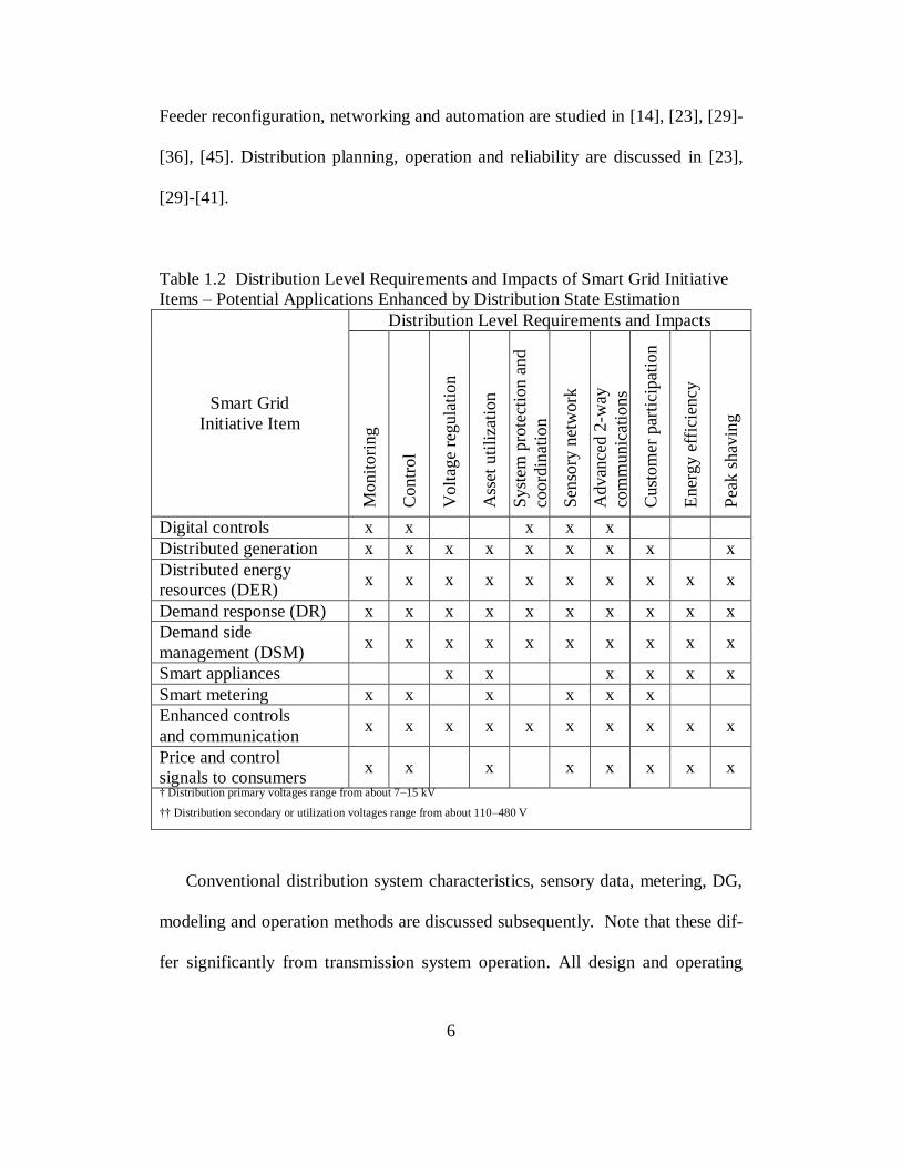
to maintain system security and reliability. Table 1.2 identifies key attributes of
the Smart Grid initiative and distribution level impacts. Challenges identified with
certain items identified in Table 1.2 are elaborated. These are motivating factors
behind the development of a distribution class state estimator.
1.5 Conventional distribution system design and operation
Designing, operating and measurement characteristics of distribution circuits
are presented before state estimation and control may be introduced. Distribution
systems interface most customer loads to the electricity supply. Unique character-
istics prevent simple adaptation of transmission modeling and analysis methods
for system studies, including state estimation. Literature on design, modeling as-
sumptions and analysis methods includes [23], [25]-[28], [45] as a small sample.
6
Feeder reconfiguration, networking and automation are studied in [14], [23], [29]-
[36], [45]. Distribution planning, operation and reliability are discussed in [23],
[29]-[41].
Table 1.2 Distribution Level Requirements and Impacts of Smart Grid Initiative
Items – Potential Applications Enhanced by Distribution State Estimation
Smart Grid
Initiative Item
Distribution Level Requirements and Impacts
Monit
ori
ng
Contr
ol
Volt
age
regula
tion
Ass
et u
tili
zati
on
Syst
em p
rote
ctio
n a
nd
coord
inat
ion
Sen
sory
net
work
Advan
ced 2
-way
com
munic
atio
ns
Cust
om
er p
arti
cipat
ion
Ener
gy e
ffic
iency
Pea
k s
hav
ing
Digital controls x x x x x
Distributed generation x x x x x x x x x
Distributed energy
resources (DER) x x x x x x x x x x
Demand response (DR) x x x x x x x x x x
Demand side
management (DSM) x x x x x x x x x x
Smart appliances x x x x x x
Smart metering x x x x x x
Enhanced controls
and communication x x x x x x x x x x
Price and control
signals to consumers x x x x x x x x
† Distribution primary voltages range from about 7–15 kV
†† Distribution secondary or utilization voltages range from about 110–480 V
Conventional distribution system characteristics, sensory data, metering, DG,
modeling and operation methods are discussed subsequently. Note that these dif-
fer significantly from transmission system operation. All design and operating

7
characteristics presented subsequently are critical aspects in the development of a
practical state-estimation algorithm.
Network design
Networked design offers operational flexibility, redundant paths, and better
service reliability [26], [29]-[40]. Distribution systems are designed as highly in-
terconnected networked systems [23]-[28]. Figure 1.2 demonstrates a convention-
al distribution network design. Primary distribution feeders are generally con-
structed as networks but operated as radial feeders via normally-open tie switches.
Networked operation is preferred for dense loads requiring high reliability; for
instance, many downtown/urban districts are operated as networks [23]-[28].
Even secondary distribution may be operated as networks [32]. Networked pro-
tection is often cited as a limitation; it is expensive and complicated to coordinate
when compared to radial system protection [26]. High voltage transmission sys-
tems are often built and operated as highly interconnected networks as they de-
mand high reliability.
Radial operation of conventional distribution systems
Radial operation is conventional in the U.S. Economics, simple overcurrent
protection, operating flexibility and the nature of loads are often cited as reasons
for radial operation [26]. Also, simplified modeling and simulation by voltage
drop calculation [25]-[27] are achieved. Radial feeders are shown in Figure 1.2.

8
Figure 1.2 An example of conventional distribution system design
High r/x ratios
The literature often identifies high r/x ratios as characteristic of distribution
systems. Significant impacts on modeling, simulation and analysis include: viola-
tion of assumptions used for fast decoupled power flows; documented instabilities
when using Newton Raphson iterative algorithms; and inability to solve networks
using DC approximations [25], [28], [42]-[45]. For example, assumptions that al-

9
low fast decoupled methods for power flow analysis are violated in networks with
high r/x ratios (namely, the assumption that line r is much smaller than x). Figure
1.3 shows r/x ratios plotted for a range of ACSR conductor sizes (cross-sectional
area in kcmils) for distribution and transmission lines; data is obtained from tables
in [28][58]. In formulating a state estimator, the calculation procedure must work
for networks with high r/x ratio conductors.
Figure 1.3 Typical r/x ratios for distribution and transmission ACSR conductors
Short run line segments serving distributed and unbalanced load
Distribution system design depends on a variety of factors including the envi-
ronment, nature of loads to be served, economics, safety and others. Generally,
most U.S. utilities use three-wire (delta, ungrounded) or four-wire (wye, multi-
grounded) circuits with a common neutral. Advantages of four-wire multi-
grounded systems include: high short-circuit currents for discrimination in over-
current relaying; inexpensive single phase service; and lower surge arrester rat-

10
ings (multiple ground paths for surge impulse) [26]. A variety of transformer con-
nections are also available. The interested reader is referred to [26].
Distribution circuits are characteristically populated by distributed loads sepa-
rated by short physical distances [26], [27], [45]-[50]. Main feeders are generally
three-phase. Laterals may be three-phase, single-phase, or consist of two-phase
conductors and a neutral. Unbalanced loading and mutual coupling between phas-
es result in unbalanced line flows and voltages during normal operation [25], [27].
In system modeling, distributed loads and short line segments increase complexity
of system models. This is significant for both power flow and state estimation al-
gorithms.
Unbalanced loads, laterals and voltage unbalance
The a priori planning method of balancing loads (MW/phase) does not entire-
ly solve the unbalance issue. Individual loads vary widely with time (stochastic),
but load types tend to follow similar patterns (correlation) [45]-[51]. The voltage
unbalance issue is problematic for utilities. Operation of three-phase rotating
equipment, effectiveness of protection systems, and protection coordination are
affected [59]-[63]. Voltage unbalance is defined by IEEE as the ratio of negative
to positive sequence voltages,
IEEE
(1.1)
Phase to sequence transformations can be found in the literature [25][28]. Voltage
unbalance may be approximated from magnitude-only calculations. One such ap-

11
proximation for voltage unbalance uses phase to neutral voltage magnitudes to
approximate, this results in higher % unbalances than obtained from Equation
(1.1),
where,
(1.2)
The National Electrical Manufacturers Association (NEMA) [63] definition for
voltage unbalance uses line-line voltage magnitudes and approximates Equation
(1.1) well for small percentage unbalance,
where,
(1.3)
Literature suggests that the approximations given by Equation (1.2) and Equation
(1.3) are valid for low values of unbalance but deviate appreciably as the percent
unbalance increases [60]. Note that Equation (1.1) includes the effect of voltage
phase angle which may be difficult to determine by direct measurement. Current
unbalance is approximately 6-10 times the magnitude of percent voltage unbal-
ance [59] [63]. More details are discussed in the state estimation formulation, and
the effects of unbalance and load uncertainty are shown in illustrative examples.

12
Low penetration of installed DG
Conventional systems have low penetration of installed DG. Penetration level
here is taken as installed capacity relative to installed feeder load. Conventional
distribution feeders have no appreciable installed DG. RPSs and grid moderniza-
tion efforts have started to change this characteristic. Monitoring, controlling and
effectively utilizing DG may become necessary in smart distribution networks.
The effective execution of microgrid strategies may depend on DG management
[65]-[69]. Tools like the DMS based state estimator may become necessary in
networks with high DG penetration.
Voltage regulation
Distribution circuit voltage regulation equipment may be sited on the feeder or
at the substation [59]. Substation equipment comprises of utility DG, capacitors,
or tap-changing (ULTC) transformers. Circuit regulators include shunt capacitors
and step voltage regulators [24]-[26]. Regulators may control each phase voltage
independently. Generally all phases of shunt capacitors are switched together.
Other options include raising primary feeder voltage, larger conductors, low
impedance transformers, load balancing, converting line sections to three-phase,
and transferring loads to other circuits [59]. A comprehensive voltage unbalance
study with regulation options is provided in [59]. Note that in conventional distri-
bution systems most DG cannot actively regulate bus voltage [45]. Distribution
state estimation may enable DG-based voltage regulation in future systems.

13
Over-current protection
References [26][28] detail distribution system protection schemes, equipment
and coordination. Overcurrent protection is employed on radial feeders. Feeder
laterals are generally protected by a fuse, recloser or sectionalizer [26]. System
protection is coordinated to ensure reliability while maintaining system security
[26]. Protection and fault-isolation has direct implication on system reliability and
related indices. Networked protection is more complex. The interested reader is
referred to [26], [28], [96].
Conventional sensors and measurements in distribution systems
Various sensors are available in the distribution system. Transmission and dis-
tribution infrastructure has a variety of applications requiring sensing: relaying
and protection, control, communication, condition monitoring, state monitoring
and maintenance. Table 1.3 presents conventional transmission and distribution
system measurements and units. Data reporting rates, communication protocols
and communication technologies are beyond the scope of this dissertation.
Table 1.3 Conventional Transmission and Distribution System Measurements
Quantity being measured Device Units
Bus voltage magnitude Potential transformer (PT) V – kV
Line current magnitude Current transformer (CT) A
Real power injections or flows PTs and CTs W – MW
Reactive power injections or flows PTs and CTs VAr – MVAr
Revenue metering Watt-hour meters Wh - MWh

14
Transducer accuracy requirements depend on the application. For example,
billing applications often utilize high-precision sensors. Lindsey presents a range
of contemporary sensors (CTs and PTs), applications and device accuracies in
[75]-[76]. Notable sensor accuracy ranges include PTs (0.3% - > 5%), [75], CTs
(0.3% -5%). These are subset of available distribution system sensors; however,
an exhaustive list may be obtained from [58], [75], [76].
In conventional distribution systems, only substation bus voltage, and line
power/current flows are available. A few main feeder current or voltage meas-
urements may also be provided. Sensor availability and placement are critical as-
pects in formulating a distribution state estimator.
Revenue metering and historical load data
Revenue metering of customer demands is done continuously. However, data
has historically been analyzed for engineering/decision making only periodically.
Customers may be charged for both energy consumed and peak usage. Previous
approaches to distribution state estimation relied heavily on historical load data.
Distribution system modeling and simulation
The characteristics of distribution circuits justify the use of different analytical
simulation tools from transmission system. The ladder iterative voltage drop
method discussed in [25] is common for distribution system analysis. Analysis of
feeders with weakly meshed networks may employ breakpoints to effectively rad-

15
icalize the system [54]. Abur in [57] developed a three-phase Newton-Raphson
algorithm capable of solving distribution networks with DG and voltage regula-
tors. Considerations include model detail / size, required solution accuracy, and
the need to model down to individual customer loads / DG. These may be im-
portant factors in developing state estimation algorithms.
1.6 The smart distribution system and need for state estimation
Areas of focus in Smart Grid initiative adaptations include: improving deliv-
ery efficiency, maximizing asset utilization, creating flexible networks and en-
hancing communication and information exchange. References [6], [14], [23],
[66], [86] present discussions of these issues. These evolving systems add sen-
sors; two-way communications; DG; responsive loads; electronic controls and
loads; and supervisory control and alarm systems for awareness [65]-[74]. Oper-
ating characteristics change as DG, switchable elements, and adequate communi-
cations permit self-sustaining microgrid islands [65]-[67]. Direct load control, re-
sponsive loads and local generation may interact to provide flexibility to operators
and customers [65]-[69].
High penetration of distributed generation and storage
Residential and commercial PV systems and small wind farms connected to
distribution voltages are DG examples [22], [23]. However, wind and solar DGs
are characteristically variable. At higher penetration levels, DG variability and

16
power flow directions may become significant [85], [86]. Illustrations to this point
are presented in later chapters.
Energy storage devices such as batteries are also likely in a smart distribution
system [67], [72], [93]-[95]. The focus of this work is system control and reliabil-
ity; therefore, storage devices are relegated to tools to accomplish control, and
elements which allow increased operating flexibility. Monitoring, control and
storage are likely limiting factors to effectively expanding DG interconnection.
Impact of solar and wind DG intermittency on distribution circuits
Distribution circuits with high DG penetration may be impacted by variability.
One notable impact of intermittency is the effect on local system voltage, unbal-
ance, and automatic voltage regulation equipment [23], [85]-[86]. Accommodat-
ing DG expansion is likely to be a major challenge for utilities. The distribution
system state estimator is envisioned as a tool to assist control and optimization of
DG and alerting operators to system issues.
Networked primary and secondary systems
References [30], [32]-[34], discuss both advantages and disadvantages of net-
worked distribution systems and impacts on reliability and restoration. Networked
operation provides superior redundancy, and therefore reliability [26], [29], [30]-
[37]. High voltage transmission systems require high reliability; consequently,
they are operated as interconnected networks.
17
Contemporary distribution systems are operated as radial feeders [25]-[27].
Normally open switches in Figure 1.2 shows how the primary voltage level may
be networked by closing switches. In this case, adaptive protection systems are
required. Cost of operating and protecting networked distribution has historically
been a barrier, high except in dense urban networks or loads requiring high relia-
bility [29]-[35]. Networked operation may facilitate higher DG penetration and
maximize asset utilization. Estimation based monitoring and control in this case
may be required.
Demand response and increased customer participation
Grid operators searching for an enhanced array of control options to help en-
sure system integrity and reliability may reach into distribution systems [14],
[87]-[91]. Improved distribution level modeling, analysis, monitoring and control
are essential to extending the opportunities for broad system control by power
system operators. Demand response (DR) is one such mechanism being explored.
Electric demand is characterized as highly inelastic in power system econom-
ics [9]-[11]. DR and price transparency in distribution networks may increase de-
mand elasticity [14], [87]-[89]. DR and conservation programs curtail loads dur-
ing high (transmission) stress periods that generally correspond to high nodal
prices [14], [87]-[91]. Direct load control, and DR options may characterize smart
distribution systems [87]-[89], [91]. Aggregating small loads and DGs to achieve
broader operational impact—also referred to as the virtual power plant—may be-

18
come viable given adequate monitoring and control. Reference [74] has identified
58,000 MW of demand response enabled load across the U.S. as of 2010.
Improved modeling of distribution networks
Better modeling of distribution systems will allow a greater degree of detail,
control, and predictable system response. Therefore operators may push the dis-
tribution system closer to its operating limits and maximize asset utilization. Ref-
erences [23], [25], [68], [85]-[86] indicate that better modeling and analysis of the
typically over-designed distribution system is necessary. An illustrative example
in Appendix A demonstrates the difference in resulting bus voltage magnitudes
comparing two different modeling assumptions.
Distribution automation
Distribution automation (DA) focuses on using technologies such as voltage
regulators, tap changing transformers and others to regulate voltages. Automated
functions at the substation level replace operator initiated action [14], [23], [68]-
[72]. Simple reconfiguration or restoration actions may be automated from the
distribution substation. The distribution state estimation application is proposed as
a supervisory DMS application. The development and implementation of an in-
formation technology (IT) layer into distribution substation operations builds on
lessons learned from transmission engineering. For instance, nascent DMSs per-

19
form functions analogous to energy management systems (EMS) prevalent in
transmission systems [66]-[72].
Smart meters and the advanced metering infrastructure
State-of-the-art revenue meters (smart meters) collect and store power, energy
consumption, and voltage magnitude data. Data may be reported directly to utility
servers at common intervals (15-60 minutes) [73], [74]. Smart meters are an evo-
lution of electricity metering; telecommunication and automation capability is
added. Smart meters have increased penetration from 4.7 to 8.7% from 2008 to
2010 [74]. Some utilities have as high as 25% smart meter penetration. Smart
meters are assumed to be a predominant sensor in the state estimator formulation
developed here.
Phasor measurements in the power system
State-of-the-art power system sensors are capable of synchronously measuring
voltages across the grid. The Global Positioning System (GPS) of satellites allows
dispersed measurement devices to be synchronized to the same clock signal. In
theory, ‘time-stamped measurements’ are compared to a single reference and an-
gular information may be determined. Details are applications to power system
are discussed in [97]-[105]. IEEE standard C37.118-2005 provides standards, def-
initions, device requirements, accepted sampling rates, data processing, measure-
ment accuracy and message format [97]. Phasor measurement units (PMUs) are

20
expected to have a major impact on power system state estimation, grid visualiza-
tion, adaptive protection systems and system operation [99]-[105]. PMUs compat-
ible for distribution systems are utilized here to formulate the estimator.
Other considerations
Other technical issues surrounding the deployment of smart distribution sys-
tems relate to: energy storage; voltage and frequency regulation; different load
types—e.g. plug-in hybrids and electric vehicles (PHEVs and EVs); energy man-
agement and optimization functions with DMS in substations; distribution auto-
mation and managing interactions of these subsystems to effectuate desired
change at the bulk power system (i.e. demand response for peak shaving, energy
storage and release for peak shaving) [23], [86], [92]-[95]. Strategies for optimiz-
ing the effectiveness of these technologies must be implemented [10], [12], [14].
Rethinking traditional distribution system operations and control may be re-
quired. For example, IEEE Standard 1547 prevents DGs from regulating system
voltages, and requires disconnection of DGs (< 10 MVA) to disconnect from the
grid during abnormal system operation [45]. Conventional operating practices,
e.g. [31]-[45], may be shown to be suboptimal. Islanding into self-contained
microgrids where local generation supplies local loads during a utility disturbance
may become practicable [65]-[67].

21
1.7 Power system state estimation
State estimation for power systems was proposed by Schweppe [106] as a way
of observing system state by fitting measurements to the assumed system model.
The first commercially operational power system state estimator was implement-
ed in AEPs system in the 1970s [100]. Today, state estimation is used extensively
at the transmission level. The state estimate provides the best fit of measurements
to the assumed system model [42], [105]-[107].
In transmission system state estimation, the state vector is taken as the posi-
tive sequence bus voltage magnitudes and angles [100]. Measurements include
bus voltages magnitudes, injections, and line flows. The estimated topology is
verified, and the static state vector is calculated. States at non-metered buses and
all line flows may be calculated. Topology processing, observability analysis, es-
timation of states, bad data processing and parameter processing are typical func-
tions of an estimator [105]. In transmission engineering, the estimator allows on-
line assessment, real-time monitoring and other applications that give operators
enhanced control.
Weighted least squares (WLS) estimation, maximum likelihood estimation
(MLE) or minimum variance estimation are common solution methods for power
system state estimation [42], [105]-[107]. The procedure assumes the network
model is known. Topology error processing bad data detection are easily accom-
modated in most state estimator algorithms [42],[105],[107].

22
1.8 Distribution system state estimation
Previous approaches to the distribution state estimation formulation are dis-
cussed in [46]-[56]. In [46] a state estimation algorithm involves constraints on
circuit quantities such as power factors, and real and reactive parts of substation
transformer currents. In the classic reference, [47] weighted least squares (WLS)
formulation for transmission systems is developed in three-phase for distribution
systems. Use of branch current state vector was shown in [48]-[49]; decoupling of
phases and increasing computational efficiency are shown. Note that bus voltages
are calculated subsequent to a converged branch current estimation.
Authors of [50] discuss distribution system modeling using voltage-dependent
load currents instead of conventional constant power loads; additionally, the au-
thors introduce the synchrophasor measurement concept to distribution. Authors
in [51] focus on modeling of loads, pseudo-loads and reliability of historical data;
where already uncertain data is presented, added heuristic reliability factors are
introduced. References [52]-[53] evaluate the choice of different estimator formu-
lations on results and modeling of pseudo-measurements respectively. In [54] an
estimation method based on the ladder iterative approach (e.g. [25]) is presented,
along with criticisms of alternate formulations as being too complex and not easi-
ly adapted to existing distribution analysis methods. [55]-[56] present applications
including topology error identification and observability analysis for distribution.
Common themes appearing in literature include real-time measurement pauci-
ty, dependence on historical load data, and large ratio of pseudo-measurements to

23
create observable scenarios [46]-[56]. An alternate distribution system state esti-
mation formulation given communications and sensory advances is presented in
Chapter 3.
1.9 Organization of this dissertation
In this research, applications utilizing distribution system state estimation are
proposed for smart distribution systems. Applications include condition monitor-
ing; reliability, reconfiguration and restoration functions; partial networking; DG
and storage management; and automation. Smart metering, synchrophasors and
bidirectional communications may be leveraged for control in the Smart Grid.
Chapter 2 contains an overview of power system reliability, restoration and
networking theory. Algorithms intended to aid distribution system planners and
operators are developed. Chapter 3 presents power system state estimation, dis-
tribution system modeling, and the formulation of a three-phase, linear distribu-
tion system state estimator. Illustrations of reliability and restoration in the Smart
Grid are presented in Chapter 4. State estimation performance is shown in Chap-
ter 5. Applications of the distribution system state estimator are shown in Chapter
6. Chapter 7 presents general remarks and concludes; appendices follow.

24
2. Distribution system reliability and restoration
2.1 Distribution system reliability
Distribution engineering is a complex science that involves striking a balance
between multiple objectives that include: power quality, reliability, efficiency,
voltage regulation, safety to the general public, environmental impacts, aesthetics
and cost. Power quality refers to the nature of the delivery voltage waveform and
minimizing harmonics and waveform distortion within the system [27], [31], [36],
[96]. Reliability is a subset of power quality and entails the continuous supply of
electrical power to the loads when needed [29]-[41].
Distribution system performance generally has the greatest effect on customer
reliability. For example, [38] indicates that approximately 80% of interruptions to
customers occur at the distribution level. Networking to provide redundant paths
and adding DG and DER tend to increase reliability, but at a cost [14], [29]-[40].
2.2 Basic reliability indices
The system average interruption duration index, SAIDI, and the system aver-
age interruption frequency index, SAIFI, are perhaps the most eminent distribu-
tion system reliability indices,
(2.1)
(2.2)

25
SAIDI and SAIFI do not capture all information relating to system reliability.
That is, they omit the magnitude of load lost during outages. These indices are
also inconsistently calculated and factors that constitute omissions vary from one
utility to another [41], [64]. Note, also, that SAIDI and SAIFI calculations ex-
clude outages shorter than 5 minutes (and severe weather events). Exact calcula-
tions and exclusions may be found in [108].
Additional similar indices are the customer average interruption duration in-
dex (CAIDI) and the average service availability index (ASAI),
(2.3)
(2.4)
Note that the ASAI and similar indices may be expressed as a ‘number of nines,’
N9, where
N9 = -log10(1-ASAI). (2.5)
Thus N9 for ASAI = 0.9999 would be 4 as an example. Equation (2.5) may be
approximated by the Taylor series expansion,
(2.6)
where a system upgraded from ASAI to ASAI + ΔASAI, results in a concomitant
increase in reliability of N9 to ; note that approximation is most accurate

26
where ΔASAI is small. This concept is depicted in Figure 2.1 where small in-
creases in ASAI, from ASAI1 to ASAI2, may be approximated by Equation (2.6).
Figure 2.1 Approximating small increments in ASAI changes with Equation (2.6)
Similarly, for SAIDI change to SAIDI ± ΔSAIDI, where ΔSAIDI is small,
(2.7)
Since these indices are system averages, they may not give information on
specific bus reliability. For specific bus reliability, load point indices are required.
The reliability measures of distribution system components or individual buses, or
load point indices [29],[30][38], can also be determined. These indices include the
average failure rate, λ (expected number of failures/year); expected outage time, r
(h); annual unavailability, U (h/y); and expectation of unserved energy, E
(kWh/outage or kWh/y), that captures the energy demanded by system loads that
cannot be delivered to those loads [38].

27
System failure rates, repair times and outage times depend on system configu-
ration and series connected versus parallel connected components. Figure 2.2
shows a system of series connected components. Figure 2.3 shows a system of
parallel connected components. System average failure rate, repair time and out-
age time are calculated in Equations (2.8)-(2.10).
Figure 2.2 System representation of series connected components
System average failure rate λS = Σ (λi) outages/year (2.8)
System average repair time rS = (Σ λi ri) / (Σ λi) hours/year (2.9)
System average outage time US = λS rs hours (2.10)
Reliability calculations for parallel components are shown,
System average failure rate λP = λ1 λ2(r1+r2) outages/year (2.11)
System average repair time rP = (r1r2)/(r1+r2) hours/year (2.12)
System average outage time UP = λP rP hours (2.13)
Figure 2.3 System representation of parallel connected components
Note that the probabilistic reliability data are based on manufacturer specifica-
tions and historical performance unique to the area of study. For example weather

28
effects, aged components and other factors affect life expectancy. Expected
SAIDI and SAIFI indices may be calculated based on Equations (2.12) and (2.13)
when the number of customers connected to each load point is known. Load
point indices may be used to evaluate relative performance of alternative system
designs, restoration plans or system topology changes. Reliability benchmarking
in a repeatable and standardized environment is discussed in [41].
Background material developed here is used to develop illustrative examples
of reliability analysis and improvement. Reliability improvement methods are
presented subsequently. Illustrative examples are shown in Chapter 4. Examples
include switching automation, reconfiguration for improved reliability and sensor
based monitoring of the electric distribution infrastructure.
2.3 Improving distribution system reliability
High reliability and fault tolerance requires multiple redundant paths, and
strategies for rapid fault detection, isolation and reconfiguration (FDIR). FDIR in
contemporary distribution systems is limited to local protection schemes which
typically do not communicate system wide activity. Thus, in order to selectively
convert existing networked distribution systems into smart distribution systems, it
is proposed to add FDIR mechanisms and automated control concepts; for exam-
ple, embedded in DMS software. The methods used shall also replicate transmis-
sion system concepts that use system restoration logic to automatically restore the
distribution system. Using circuit matrix concepts, the optimization of the relia-

29
bility at system buses shall be performed based on the reliability of individual
components. Illustrative examples and discussion are provided in Chapter 4.
2.4 Distribution system restoration
Distribution system restoration is concerned with reenergizing feeders / loads
that have experienced an outage. Transmission system restoration following a ma-
jor outage is widely covered in the literature. However, references [108], [110]-
[115] provide comprehensive coverage of distribution and transmission restora-
tion. Transmission system restoration is critical following major grid disturbance.
Expediency to allow load restoration; it is concerned with black-start generation,
island synchronization then full system restoration. Many restoration functions
rely on heuristics. Digitizing restoration functions is one aspect of distribution au-
tomation [24]. The foundation for developing a continuous running process to
sensing when to restore is presented subsequently.
The size (e.g. MW) and duration of the outage are critical aspects to distribu-
tion system restoration; additionally, restoration time drastically affects expecta-
tion of unserved energy. Small, short duration outages are less problematic.
However, if an entire distribution feeder has been de-energized for an hour, resto-
ration includes cold-load pickup and inrush currents which become problematic
for system protection; a more careful reenergization plan must be undertaken [26],
[112]. Pre-outage loading, cold-load pickup effects, and available network topol-
ogies are critical aspects to distribution restoration. As a small example, consider
a substation transformer serving 5 MVA on a radial feeder. A lateral serving 200

30
kVA experiences a fault and subsequent outage lasting 20 minutes: the
reenergization plan may be simply to replace a blown fuse or switch to an alter-
nate source to restore normal operation. This looks like a small positive step
change in loading at the substation.
References [33], [36], [96], [109]-[116] identify challenges to distribution sys-
tem restoration. Outage detection and restoration may be categorized: outage de-
tection and location; data gathering via customer calls and SCADA systems; visu-
al inspection for outage cause verification; take action to restore system from out-
age [116]. References [109]-[116], discuss distribution system restoration issues
that include, but are not limited to, cold load pickup, transformer thermal behavior
and optimizing restoration order. Discussions of restoration methods indicate that
a combination of different techniques such as analytical, heuristic and knowledge-
based systems are used to effect restoration.
Distribution system design should enable reconfiguration and restoration func-
tions that improve reliability. Restoration may be objectively formulated, for ex-
ample: reduction of SAIDI (duration index), minimization of expected unserved
energy to loads, minimization of switching commands. A simple algorithm aimed
at reliability monitoring and restoration assisting is provided in [117].
2.5 A network theoretic approach to distribution system reliability
An overview of graph theoretical concepts is presented in the next few para-
graphs. The application of graph theory to the power distribution system is ex-
plained, and algorithms exploiting graph theoretical concepts are developed.

31
The physical layout of a power system may be represented by a set of
nodes/buses, connected by a set of edges/branches/lines) [120]-[122]. From graph
theory, a graph is an ordered pair consisting of a set of nodes, n, and a disjoint set
of edges, e, that can be mathematically characterized by an incidence function –
usually a matrix – that associates nodes with edges. Edges emanating from or ar-
riving to a node are referred to as incident to a node. Branches may form loops,
be parallel branches, or connect adjacent nodes.
Directed edges are specified as leaving one node and arriving at another; such
a system is called a directed graph, or digraph. A symmetric digraph has bi-
directional edges connecting nodes and may be treated as undirected [120]. Undi-
rected graphs cannot have loops (a branch leaving and arriving at the same node).
Figure 2.4 (a) and (b) show a digraph and undirected graph respectively. A power
system can be represented as an undirected graph, where nodes / buses are con-
nected by branches.
A path refers to a graph whose nodes are both linearly and sequentially con-
nected, generally by a directed walk connecting from-node and to-node. In Figure
2.4 (a), the path {a, b, c, d, a, a} is connected by directed walk {1, 2, 3, 4, 5}.
When all nodes are distinct a directed path exists, with length defined as the
number of edges. Figure 2.4 (a) shows the set of directed walks M = {1, 2, 3, 4,
5} which is a 5-path digraph connecting the set of nodes {(a, b), (b, c), (c, d), (d,
a), (a, a)}. Figure 2.4 (b) shows a 4-path undirected graph, where walks complete

32
path {w, x, z, y, w}. Both graphs are referred to as connected graphs since all
nodes are simultaneously connected through edges. A connected graph contains
at least one path between all distinct nodes. Power systems are generally repre-
sented by connected, undirected graphs (as in Figure 2.4 (b)). Subsequent discus-
sions will refer to nodes as buses and edges as branches.
Figure 2.4 (a) A directed graph; (b) an undirected graph
If all buses in the graph are not connected, it is referred to as a disconnected
graph or a component of the graph. In a power system, this corresponds to island-
ed systems. Matrix representation of graphs may be used for modeling and analy-
sis [121]. Modeling the power system is accomplished through graph theoretical
concepts such as incidence, J, and adjacency, A, matrices. The incidence matrix of
a graph with n nodes, and e edges is of size n x e with entry 1 if a bus is connected
to a branch and 0 otherwise. The adjacency matrix, A, is of size n x n, where en-
tries are 1 if buses are connected, 0 otherwise. J and A for Figure 2.4 (b) are,

33
J here is an unoriented incidence matrix since the graph is undirected.
As discussed, the distribution system may be represented as an undirected,
connected graph, where matrices constitute bus and branch connectivity. Power
system applications are particularly interested in how removal of a branch or bus
impacts the system. Power system data comprise branch connectivity (from-to
bus), branch impedance, and location of generators and loads. Power system
models (Y-bus) are constructed via adjacency and incidence matrices. The subse-
quent discussion uses binary representation of graphs, and of the adjacency and
incidence matrices, in power system applications.
2.6 The binary bus connection matrix
A binary connection matrix, B, is used to model the distribution system for
connectivity for reconfiguration applications. Branches are modeled as ones
when energized and zero otherwise,
Connectivity for an n bus system entails raising B to higher powers; the matrix Bn-
1 will contain all ones except in positions ij where i and j are not connected to each
other through any number of intervening buses. Thus a zero entry in Bn-1
identi-
fies buses that are not energized [44]. B is an n x n matrix containing binary en-
tries. Powers of B are found using Boolean operations, e.g.,

34
where and are Boolean OR and AND operators respectively. Circuit break-
ers and switches are represented as ones when closed and zeros when open.
2.7 Application of B matrix to power system reliability and restoration
Powers of the B matrix (i.e. Bn) allow tracing network connectivity. Analysis
of proximity (how close one bus is in relation to another via number of lines), de-
gree of connectivity (how many lines connect two buses), and the calculation of
intervening buses between two buses [44]. As discussed, in a system with n buses,
Bn-1
contains all ones for a fully connected system. Zeros in the matrix identify
disconnected, and therefore, deenergized buses. Additionally, By for an n bus sys-
tem contains ones only when buses are connected by y lines or less, for y< (n-1).
Evaluation of the calculation shows that there are y-2 intervening buses. Assess-
ment of network connectivity may be used to evaluate reliability and build resto-
ration algorithms. Chapter 4 presents illustrative examples of B matrix applica-
tions in reliability assessment.
Advantages of using the B matrix include the use of Boolean arithmetic to lo-
cate energized (or deenergized) buses. An example of distribution system appli-
cation to reliability enhancement may be the minimization of unserved energy
after a component failure and consequent reconfiguration. The B matrix allows
energized loads, line segments and buses to be identified; consequently, near op-
timal network reconfiguration may be performed. Figure 2.5 outlines steps in
which the B matrix is used in a distribution system reconfiguration / restoration
algorithm. Application areas include design – to optimize placement of interrupt-

35
ing devices (breakers, reclosers, switches, electronic switches), or operations – as
a method to automate circuit reconfiguration and restoration. Additional com-
ments on this algorithm and elements of Smart Grid operation are shown in [118].
Figure 2.5 B matrix algorithm to be used in distribution system applications
The B matrix provides a foundation for the circuit connectivity analysis. Load
diversity, daily load profile and seasonal load profile patterns require robust de-
sign and operation methodologies. The B matrix can be used in a running real-
time control application that inputs sensory information about the system into an

36
algorithm that can enhance automated restoration and reconfiguration ability. For
example, sensors in the distribution circuit can monitor real-time demand infor-
mation and use these measurements to minimize the unserved energy in the event
of an interruption. Figure 2.6 shows the elements of a potential application em-
bedded in a DMS with the proposed concept of real time monitoring / sensing /
reconfiguration / restoration calculation for distribution systems.
In circuit design applications, it is possible to compare alternative locations of
interruption devices, switches, sensors, and circuit routing in order to achieve a
given objective. In distribution design, the long list of objectives may include:
loss mitigation, high reliability of service, voltage regulation, operation within
component ratings, public acceptance, safety, compliance with standards, and sat-
isfying cost constraints. In a subsequent example and discussion, Chapter 4 illus-
trates applications of an algorithm to ‘seamlessly’ reconfigure the system and re-
store service. In design and operation applications, possible objectives include:
Reducing the SAIDI and SAIFI (reducing outages < 5 min.)
Reducing expectation of unserved energy after a permanent fault
Restoring maximum permissible load after a circuit disturbance.
Note that maximum permissible load may be connected MVA or pre-disturbance
demand. Figure 2.8 presents a detailed flowchart comprising sensory information,
operator alerts and automated reconfiguration / restoration of distribution systems.
In an algorithm utilizing the binary bus connection matrix, B, a system status
table (SST) can be assembled as depicted in Figure 2.7 where ncb, nb, and nl de-

37
note the number of breakers, buses and lines respectively. This SST is constructed
based on the physical system structure and binary representation of breaker states,
bus states, load states and line availability.
Figure 2.6 Sensing and real time monitoring of distribution system elements for
computer assisted calculation and control
Figure 2.7 System status table indicating status of breakers, buses, lines and loads
Breaker states, bus status, load status and line availability are represented by
zeros and ones. That is, closed breakers / switches, energized lines, loads, and
buses are represented by ones; conversely, open breakers, deenergized lines,

38
loads, buses are represented by zeroes. Note, however, that the number of rows in
the table increases as the number of interrupting devices, ncb, increases according
to . In practical implementation, the number of automated interrupting de-
vices within a distribution system remains low.
The restoration of a distribution system based on a table lookup method is dis-
cussed. The method is outlined as follows:
First, communicate the status of all circuit breakers and availability of ser-
vice at load buses every ΔT seconds.
Next, the SST is updated as needed every ΔT seconds. Note that if a line
was faulted or some distribution system device was unavailable, the corre-
sponding row of the SST would be removed.
Then, detected anomalies trigger examination of the remaining rows of the
SST. The desired state lies inside the set of remaining rows. To select the
desired target row, apply an optimal operating criterion; for example, as
indicated in Table 2.1.
The restoration algorithm of Figure 2.8 is repeated every ΔT seconds.
2.8 Sensors for reconfiguration and restoration
Note that ΔT depends on the sampled data and applications for which it is
sampled. For example, ΔT of 5 minutes or less allows for switching that can sig-
nificantly reduce reliability indices according to [123]. Also, recall that only in-
terruptions lasting more than 5 minutes are considered when calculating SAIDI.
The 5 minute sampling rate is well within contemporary technology, as SCADA

39
data are updated every 4 seconds and state estimation at the transmission level
runs every 2-3 minutes [103].
Figure 2.8 An automated restoration / reconfiguration algorithm
Table 2.1 Sample Optimal Operating Strategies for Restoration
Strategy Objective
Minimum breaker
operations
Minimize the number of switching operations, to
accelerate the restoration
Maximize load restored Restore large loads first, to minimize energy un-
served (knowledge of load priorities may be needed)
Minimize unserved energy Examine all permissible switching operations and
choose those that minimize the unserved energy
Priority loads first Restore priority loads first, regardless of load level
Under more stringent conditions, ΔT may be ½ cycle or 8.3 ms to stay within
the Computer Business Equipment Manufacturers’ Association (CBEMA) curve

40
requirements [36]. In this case, virtually no momentary interruption event con-
tributes to SAIDI and SAIFI indices. Additional consideration is given to the sen-
sory network required of the Smart Grid environment. Type of available meas-
urements and application areas are presented in Table 2.2.
Table 2.2 Quantities Sensed for Distribution System Restoration
Sensed quantity Purpose
Bus voltages On/off
Acceptable service delivered
Bus injection current
On/off
Load level before disturbance
DG supply before disturbance
Line flows (real power,
reactive power, current)
Compare actual levels to equipment limits
Evaluate available paths
Breaker/switch status On/off
Available/unavailable
Generation set points
(DG)
Evaluate system supply to identify available paths
Identify available reactive support sources
Load operating point be-
fore disturbance or out-
age
Important in understanding how much load needs
restoring
Important for restoration involving cold-load
pickup
Ambient / equipment
temperatures
Detect overloaded or overheated equipment
Find conductors that may be sagging excessively
Transformer temperature
/ pressure Detect overloaded or overheated transformers
Fuse status Reduce restoration and repair times by conclu-
sively locating and addressing faulted components
Lightning arrester and
protective device status Locate and repair protective equipment that failed
while protecting the circuit

41
3. A distribution class state estimator
3.1 State estimation in the distribution system
Utilizing measurements to estimate the state of the power system has been
used extensively at the transmission level as discussed in Chapter 1. Generally,
the assumed system topology and SCADA data are combined with redundant
measurements and reasonable assumptions based on previous operating points.
Note that assumed data points may be derived from solved power flow solutions,
historical data, and previously estimated solutions. Again, measurements include
real and reactive power injections and flows, bus voltage magnitudes, and relative
phase angles where phasor measurements are available. Solution of the estima-
tion procedure provides state estimates where no measurement devices exist.
The state estimation process generally employs non-linear solution methods to
iteratively find a least square approximation to an overdetermined problem [105].
Generally, the non-linear solution employed is the same as the Newton-Raphson
technique used for power flow analysis, except for the measurement Jacobian de-
scribing the non-linear relation of the states to measurements. As discussed in
Chapter 1, distribution systems have different characteristics that prevent simple
transfer of modeling and analysis methods. Examples identified in Chapter 1 in-
clude high r/x ratios, radial configuration, two and single phase laterals, and un-
balanced loading. Distribution power flow studies often utilize a robust ladder it-
erative technique [25] to find bus voltage profiles and current flows for radial sys-

42
tems. Considering the various requirements, a practical distribution system state
estimator is developed subsequently.
3.2 Applications of a distribution class estimator
State estimation may be used to enable control functions in a number of sce-
narios. For example, comparing estimated flows and voltages to ratings or
switching to prevent component overload. Applications of a distribution class
state estimator enable smart distribution system initiatives. A list of potential
benefits includes:
Optimization and generation rescheduling based on forecasted state,
Enhanced system wide voltage control capability,
Single phase VAR control to facilitate voltage regulation and utilize DG,
Enabling voltage regulation via local DG,
Selective networking of primary and / or secondary systems for voltage
control, loss minimization, or increased asset utilization,
Facilitate real-time distribution level pricing based on congestion/flows,
Energy storage management and optimization,
DG location and control – i.e. to relieve congestion, manage prices,
DMS that provide operators more effective distribution feeder interaction
tools; i.e. monitor and visualize the grid like transmission systems, alarms
and alerts of serious events,
Enables control signals for demand-side-management of smart appliances,
PHEVs and responsive loads,

43
Enable demand response that truly impacts bulk grid operations, e.g.
switch appliances to ‘reduced demand’ mode when directed,
Fault detection (not protection), isolation, and reconfiguration for en-
hanced reliability,
A validation tool– load and topology –for transmission system state esti-
mators.
3.3 Synchronized phasor measurements in power system state estimation
Synchrophasors in state estimation is seen as revolutionary, since system
states (bus voltage magnitude and angle) may be directly measured [77], [100],
[102]-[104]. The application of synchrophasor measurements in distribution sys-
tems and distribution state estimation enables direct measurement of system states
as well; however, direct measurement of three-phase unbalanced voltage magni-
tude and angle provides a significant amount of information to the distribution
operator. This is particularly important, since most operators only have substation
SCADA data to gauge feeder conditions [68]. Although wide deployment of
measurement devices with synchrophasor technology is envisioned, even a few
such measurements combined with smart meter data and other measurements may
enhance the feasibility of distribution class estimators.
Additionally, the ability to visualize the grid enables more effective control
and optimization strategies. For example, capacitor bank switching based on
measured / estimated voltage profiles may become more effective than conven-
tional time-of-day switching. Also, effectively utilizing available resources, i.e.
44
reformulating portions of the IEEE Standard 1547, to allow islanded / microgrid
operation where available DG capacity can supply local loads. Knowledge of
contemporary system conditions allows operators to push the distribution system
closer to its operating limits.
3.4 Conventional state estimation formulation
The process of state estimation in transmission systems involves the use of
measurements along with a mathematical system representation to obtain least
squares fit of estimates to the assumed topology. General assumptions that allow
the use of positive sequence equivalent circuit models to estimate the positive se-
quence states include:
System topology is known (or processed to within an acceptable limit),
Balanced three-phase loads,
Fully transposed lines,
Symmetrical series or shunt devices on all phases,
State estimation uses a large number of redundant measurements. Where an
insufficient set of measurement data exists, historical data (i.e. pseudo-
measurements) or virtual measurements (i.e. zero injections) may be substituted to
obtain an observable / non-singular process matrix [42], [105]. States may be rep-
resented as polar or rectangular quantities. At a given operating point, the non-
linear relationship of measurements to states is given by Equation (3.1),
h(x) = z’ +η, (3.1)

45
where z’ and η are vectors of measurements and measurement errors respectively,
x is the vector of system states (bus voltage magnitude and angle), and h is a non-
linear vector valued function that relates system states to corresponding measure-
ments. Typically the power system state estimation problem presents itself as an
overdetermined system where redundant measurements outnumber states.
Weighted least squares estimation involves the minimization of the 2-norm of
the residual vector denoted by r, z = (z’+η) is the noisy measurement vector,
r = (z’+η) – h(x) = z – h(x) (3.2)
Quite often, the 2-norm of the residual vector is taken as the objective function,
given by the non-linear objective function, J(x),
where k is an arbitrary bus number and n is the number of measurements. Note
that as the summation of the square of residuals of individual measurements, J(x)
is a scalar. The minimization of J(x) entails equating the partial derivative of J(x)
with respect to the state vector, x, to zero,
. (3.4)
That is, the minimization of J(x) simultaneously minimizes each measurement
residual.
Power system state estimators utilize a large number of redundant measure-
ments. Mathematically, state estimation becomes an overdetermined system of
equations. Where data may be linearized around an operating point, Equation
(3.1) becomes
, (3.3)

46
hx = z. (3.5)
Consequently, Equation (3.2) may be written as,
r = z – hx. (3.6)
For an overdetermined system of equations, the best-fit estimated solution to
Equation (3.4), linearized to produce Equation (3.5) – (3.6) is given by,
2hth – 2hz = 0
= [hth]
-1 h
tz (3.7)
Note that this result may also be found as,
= h+z, (3.8)
where h+ denotes the Moore-Penrose pseudo-inverse where h is of dimension n x
m , n > m.
Note that in conventional transmission system state estimation, the state vec-
tor denoted is a real valued vector with magnitude and phase information parti-
tioned into sub vectors.
3.5 The gain matrix in power system state estimation
In the conventional power system state estimation formulation, there typically
exists a gain matrix that provides weights for measurements. Measurement de-
vice accuracy and measurement type are common weighting attributes. Types of
measurements include:
Measured: low variance (high weight); corresponds to meter accuracy
Virtual measurement: low variance (high weight) e.g. zero injections

47
Pseudo-measurement: high variance (low weight), assumed values
Critical measurement: pseudo, virtual or measured; to avoid singularity.
For example, the accuracy range for various PTs is presented in Chapter 1. Pseu-
do-measurements are assumed from historical data, thus, they are less reliable
than metered node measurements. The gain matrix allows a solution procedure
where reliable data dominate the solution subject to acceptable system condition.
The covariance matrix of the measurement vector is denoted by R. If the
measurement variances are assumed to be independent, R is a diagonal matrix
with entries corresponding to measurement variances; that is, when individual
measurement variances are assumed to be independent, the off-diagonal terms are
zero,
It is possible to weight the calculation of each measurement residual in J(x). In
this case, the matrix, W, is calculated as the inverse of the R matrix. A low vari-
ance corresponds to a high weight. Linearizing Equation (3.4) around the state
vector by Taylor series expansion, one obtains correction terms to initial esti-
mates. This enables an iterative solution to the non-linear set of measurements in
conventional state estimation, similar to the calculation of the Jacobian in Newton
Raphson power flow solutions. Incorporating W into the system of equations pro-
duces a gain matrix, G,
G =h ast
W hmeas . (3.9)

48
hmeas represents the subset of the h matrix relating system measurements to the
state variables. The solution to obtain the x vector in Equation (3.8) is then modi-
fied to produce,
= [G]-1
htWz . (3.10)
References [42], [104]-[107] provide further discussion on weighted least squares
estimation and the gain matrix.
3.6 A three-phase, linear distribution system state estimator using synchro-
nized phasor measurements
The three-phase, untransposed distribution system requires a different set of
tools capable of estimating all phase voltage information. The formulation devel-
oped utilizes complex synchronized phasor measurements and complex mathe-
matical representation of state estimation equations. Note that in the case where
synchronized phasor measurement devices are utilized, it is possible to obtain real
and imaginary components of measured quantities. The foregoing formulation
may be modified to accommodate complex measurements. For such measure-
ments, the equations within the h matrix, measurements in the z and η vectors, and
state vector are represented as complex quantities. Consequently,
h = hr + jhim,
z = zr + j zim,
x = xr + jxim.
Each matrix or vector can be partitioned into real and imaginary subsets denoted
by the subscripts r and im respectively. To accomplish the minimization of equa-

49
tion (3.3) for a complex vector, r = rr + rim, the partial derivatives of the system
of equations with respect to real and then imaginary variables must take place
simultaneously. When the n, x and z vectors and h matrix are complex, the result-
ant r vector minimization given in Equation (3.4) requires complex conjugation
followed by transposition for the equation to be minimized,
rHr = (zr – hrxr + himxim + ηr)
2 + (zim – himxr – himxim + ηim)
2. (3.11)
The Hermitian operation is transposition, followed by complex conjugation, and
is denoted (•)H.
The expression of the minimization of the complex expression becomes,
(3.12)
In commercially available software programs such as Matlab, the Moore-
Penrose pseudo-inverse function correctly computes the pseudo-inverse of a ma-
trix entered in complex form. The residual vector may be separated into its re-
spective real and imaginary parts, the result is,
The solution for the estimation of state variables, , when variables are in rec-
tangular form,
Note that and m are independent of each other. Estimation of sequence val-
ues follows the same formulation previously described. Phasor measurement de-
(3.13)
(3.14)

50
vices measure individual phase values, and calculate positive, negative, or zero
sequence components.
Note that the 2-norm minimization of the complex quantities has real r vector,
and that Equation (3.12) can be solved using Equation (3.8). Also, hHh is a square
matrix and, provided it is not singular, may be used to solve the state estimation
problem. Measurement weights may also be included. This point is discussed in a
later subsection.
The preceding formulation may be developed for three-phase networks.
Where synchronized phasor measurements are available, the real and reactive part
of the measured quantity may be calculated (since magnitude and angle infor-
mation are effectively measured). In conventional state estimation formulation,
the process matrix and gain matrix grow by a factor of 3. Also, as in conventional
power system state estimation, measurement weights of synchronized phasor
measurements are generally higher than other measurements since these devices
are generally assumed to have a higher degree of accuracy.
3.7 Three-phase radial distribution ladder iterative power flow
Three phase voltage profiles for radial distribution feeders are generally ob-
tained via a ladder-iterative algorithm, also called the forward / backward sweep
method. Algorithms detailing the forward sweep and backward sweep are pre-
sented in Appendix B. Calculating voltage and current at node n when values at
node m are known may be accomplished for most distribution system components
–lines, transformers, regulators– using a generic formulation,

51
This system may be solved when bus voltage and currents are known. Note that
in conventional distribution systems only substation bus voltage magnitude and
possibly line current magnitudes or power flows are measured. The A, B, C, D
matrix in Equation (3.15) is inverted to solve for bus m quantities when bus n
quantities are known. Note that for a given line topology, the unit quantities (e.g.
Ω/mi.) remain constant; consequently, the inverse of A, B, C, D may be per-
formed once for each line topology and stored. The forward iteration solves for
bus voltages at successive downstream buses when an upstream bus voltage and
branch currents are known. The backward stage solves for upstream voltages at
successive buses when downstream bus voltages and line currents are known.
Both forward and backward iterations assume current entering a branch is the
same as current leaving a branch.
The untransposed line segments with high r/x ratio (e.g. three-wire or four-
wire) are modeled with an n_ph square matrix where n_ph is the number of phas-
es (typically 3). Four-wire segments are reduced to a 3 x 3 block matrix using
Kron reduction by assuming neutral conductors are solidly grounded at every
node [28]. For Figure 3.1, line segment impedance (effective line-ground after
Kron reduction for 4-wire) matrix between buses n and m is,
(3.15)

52
Where a single or two phase lateral is present, the row and column of the
missing phase(s) are zeroed, and the corresponding voltage vector entries in
in Equation (3.14) are zero. Similarly, transformers are modeled by an n_ph x
n_ph block impedance where diagonal elements represent phase self impedance;
taps and delta-wye connections may also be modeled [25]. The modeling as-
sumption for transposed transmission lines that allows use of the positive se-
quence impedance effectively averages off diagonal elements, Zm = 1/3(Zab + Zac
+ Zbc).
Bus n Bus ma
b
cn
a
b
cn
g
Z nm
abc
g
Figure 3.1 Line impedance between buses n and m
Quite often the same approach of averaging off-diagonal elements is used in
the ladder iterative power flow but results in loss of solution accuracy. The stop-
ping criteria for forward / backward sweep may be tolerance, e, around balanced
substation voltages, , (as substation bus voltage magnitude
may be the only measurement available).
The three-phase unbalanced distribution state estimator developed henceforth
combines techniques from the ladder iterative algorithm to process measurements,
and to find reasonable solutions for non-measured quantities. Also, reasonable
estimator inputs may be obtained via measurements and supplementary calculated
system quantities.

53
3.8 Three-phase unbalanced distribution state estimation
The general procedure for the pre-processing and state estimation algorithm is
depicted in Figure 3.2. The two stages of the estimation procedure are a ladder
iterative process followed by linear estimation. This is intended to provide a pre-
processing method to obtain missing measurements in an environment where lim-
ited measurements may be available.
Figure 3.2 Three-phase unbalanced distribution state estimation overview

54
Where smart meters are available, real and reactive power consumption, as
well as voltage and ampere magnitudes may be obtained at the customer load.
When the clock on the smart meter is synchronized to some general reference,
these quantities may prove coincident peak and near real-time voltage magnitude
measurements. However, fully synchronized measurements that provide angle
information are not likely to be available from the smart meter. Development of
such devices to be included in next generation smart meters, protection systems
and distributed generator protection and control may enhance distribution state
estimation efforts. Additional discussion may be found in [134].
3.9 Condition number and state estimation
To assess the accuracy of solutions to the state estimation problem, certain
concepts in linear system and matrix theory must be introduced. References
[124]-[126] present matrix theory as applied to linear algebra and numerical anal-
ysis. Matrix theory applied to power system state estimation is discussed further
in [105]-[107] and is discussed subsequently.
The vector norm is a scalar that measures the length or magnitude of distance
between two vectors in the same fashion that absolute value measures the length
of a line [124]-[128]. Norms must meet three criteria: positivity, homogeneity,
and triangular inequality (as explicitly detailed in either reference). The most fre-
quently cited vector norm is the Holder norm,

55
n = number of elements in the vector
xi = the ith
element in the vector
p = 1, 2, 3 … ∞.
(3.15)
||x||p is referred to as the p-norm. Note that p=2 in Equation (3.15) is the Euclidi-
an norm, or 2-norm, also utilized in the weighted least squares formulation.
Vector norms are often used to evaluate the difference between a calculated
solution, , and the exact solution, x, which is rarely known. The error is given
by e = x – . The basis of state estimation is the minimization of the norm of Ax –
b. If for a given matrix, A, there exists a nonzero vector, x, for which Ax = λx,
then λ, is an eigenvalue of A, and x is an eigenvector of A associated with λ. The
collection of all individual eigenvalues of A is known as the spectrum of A. The
spectral radius of A is the maximum absolute value contained within the spectrum
of A. Reference [124] identifies a disadvantage of using the spectral radius to
measure the size of a matrix: i.e. when two matrices, A and B, have spectral radi-
us , as this condition violates the triangle inequality.
Often used norms are calculated as,
2-norm or Euclidian length
(3.16)
Infinite norm
(3.17)
As summarized from [105][124]-[128] the condition number of a matrix pro-
vides a measure of how small perturbations in the right-hand-side of Ax = b may

56
become magnified in the calculated solution of to produce meaningless results.
The condition number of a matrix is calculated via
κ(A) = ||A|| ||A-1
|| (3.18)
In conventional state estimation, A indicated above is hth. That is, the h
th ma-
trix is nearly singular in some cases. Three situations cited for causing ill-
conditioned power systems are identified as large weighting factors to certain
measurements, short and long lines connected to the same bus, and a large num-
ber of bus-injection measurements [104][105]. In the state estimation formula-
tion, it is expedient to examine the condition number of hth which is obviously
square and symmetric. The condition number of this formulation may also be cal-
culated exactly by the ratio of the maximum to minimum singular values of hth,
κ (hth) = smax / smin . (3.19)
Note that singular values are always non-negative real numbers. As identified in
[105], the formulation of the conventional power system (transmission) state es-
timation problem is naturally ill-conditioned.
In power system state estimation, the condition number effectively gives the
sensitivity of the solution to noise in the measurements. When the condition
number is very large, there is a high sensitivity to noise. In traditional power en-
gineering applications, literature cites condition numbers less than 1012
as normal-
ly encountered in practice [129].
The foregoing discussion of condition number in general, and in the tradition-
al power engineering state estimator cases may be recast into the proposed distri-

57
bution state estimation solution given by Equation (3.8). The recast expression
replaces h in Equation (3.19) by
.
The condition number is then calculated as,
. (3.20)
Note that in Equation (3.20), all elements in the argument of the condition number
calculation are real, and the argument is a square matrix.
The condition number for the distribution state estimator shall be revisited in
connection with illustrative examples in Chapter 4. It provides a reasonable esti-
mate of the sensitivity of the state estimation formulation to measurement noise
and system model error. Further discussion of condition numbers and matrix con-
cepts is provided in Appendix C.
3.10 Assignment of weights to calculated currents
As discussed in subsection 3.5, a weight assignment process biases calculation
of states toward data identified as more reliable. In the distribution system state
estimation algorithm developed here, load currents are linearized. The currents
calculated are written in linear expressions in terms of the states, namely the bus
voltages in rectangular notation. Substation active and reactive power flows may
be expressed in terms of real and imaginary part of currents which are also linear-
ly related to the states, particularly since substation bus voltage magnitude is

58
known. Measured values (i.e. from a smart meter) generally include active and
reactive power, S = P + jQ, and voltage magnitude, |Vm|. Synchrophasors provide
voltage magnitude and phase angle relative to a reference.
Assuming small change in nominal bus voltage phase angle obtained from the
power flow solution, the current demanded by a load may be calculated. For ex-
ample, a constant power load current may be represented as,
(3.30)
(3.31)
where φ denotes the phase (a, b, c) and voltage phase angle, δv, is assumed near
nominal for that phase (i.e. 0o, -120
o, 120
o respectively) when not measured di-
rectly via a synchrophasor. If measured via synchrophasor, the measured may
be used. Alternatively, phase angle information of nearby measured buses may be
used as an initial estimate where no measurements / pseudo-measurements exist.
Other load models may be employed. Note that constant impedance, constant cur-
rent or composite load current may be calculated similarly [25], [46], [53], [57],
[85]; additionally, models calculating current as a polynomial in terms of the volt-
age magnitude may also be included [59]. Field tuning of load models may be
required for verification, especially for power flow study accuracy. At the operat-
ing point, the voltage and current relationship is simply YV = I.
The selection of weights for calculated, linearized currents may be approximated
mathematically or determined heuristically. Measured P, Q, Vm and δv are random

59
variables each with an expected value and variance [132]. Approximate expres-
sions for mean and variance of calculated currents from Equation (3.31), may be
obtained when measurements are treated as independent random variables. The
expected values of measured variables are Mk = {P, Q, Vm, δ}, and their variances
=
δ
are chosen based on transducer expected accuracy.
Transducer expected accuracies for typical power systems sensors are discussed
in subsection 1.5 and of an example of a commercialized product is shown in
[97]. Attention now turns to the approximation of variance of the calculated cur-
rent.
The expectation of real and imaginary parts of I, are calculated in Equation
(3.31). In statistics theory, these calculated values represent expectation of real
and imaginary parts of current, respectively. The expectations are said to
be approximated from the nonlinear functions in Equation (3.31). The variance of
Ire and Iim are approximated from the Taylor series expansion, also commonly re-
ferred to as the ‘delta method’ [132], evaluated at for each measurement (as-
suming independent measurement noise, Mi = {P, Q, Vm, δ}),
a
n .
a
n .
(3.32)
Alternatively, a heuristic approach may be taken: the variance of Ire and Iim
may be approximated by choosing a value corresponding to the largest variance
(normalized) of all random variables, i.e., truncate the sum in Equation (3.32) to

60
only the largest term(s). Note that calculated variance of the real and imaginary
parts may differ significantly. Appendix D presents an illustrative example of ap-
proximating calculated current variance, as well as confirmation of the heuristic
method described.
3.11 Bad data detection and the distribution system state estimator
Other applications of estimators for distribution systems include topology er-
ror identification, and a variety of operations dealing with bad data detection,
identification, suppression, and correction. Baran et al. demonstrate the identifi-
cation of incorrect modeling assumptions in [56]. Powalko et al. provide an analy-
sis of the observability issue for a distribution network estimator in [55]. Abur’s
text [105] details algorithms for bad data detection. One illustration using chi-
squares is explained briefly below.
Bad data detection and identification filters the measurement set for erroneous
data. The bad measurement must not be a critical measurement (that makes the
mathematical set of equations observable) [105]. Observability in this context
means that the state estimation matrix h is such that hth is nonsingular. Bad data
detection and identification for the linear, three-phase distribution system state
estimator formulation follow methods outlined in the literature for WLS estima-
tors (e.g. [105]). An illustrative example is presented in Chapter 5. The individual
measurement errors are assumed to follow a normal distribution, are independent
and uncorrelated.

61
4. Illustrations of reliability enhancement in the Smart Grid
4.1 Reliability and the Smart Grid: test cases for reliability enhancement
and restoration strategies
In this chapter, a key focus of the Smart Grid is presented – namely reliabilirty
enhancement and distribution restoration. The objective is to use enhanced senso-
ry information to improve reliability and to implement restoration. The approach
taken is mathematical and illustrative (i.e., through the use of examples). The
same sensory utilization approach will be the foundation of distribution system
state estimation, the subject of the subsequent chapter.
Various test cases are used to illustrate the several algorithms that have been
developed here. Standardized test beds provide a platform upon which compara-
tive studies can be conducted, and where calculation results of different alterna-
tive methods or designs (i.e. to different reliability designs or switching strategies)
can be obtained. Table 4.1 identifies the test beds used and related illustrations.
Note that the names, number of examples / simulations, and more specific details
are presented in each subsection.
Table 4.1 Examples Presented in Chapter 4
RYG Test Bed RBTS Test
Bed (1-line)
Binary bus connection matrix x x
Restoration x
Reliability enhancement / automation x
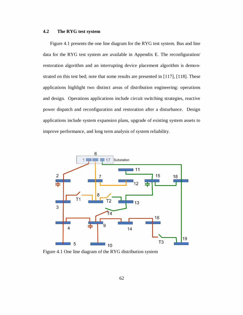
62
4.2 The RYG test system
Figure 4.1 presents the one line diagram for the RYG test system. Bus and line
data for the RYG test system are available in Appendix E. The reconfiguration/
restoration algorithm and an interrupting device placement algorithm is demon-
strated on this test bed; note that some results are presented in [117], [118]. These
applications highlight two distinct areas of distribution engineering: operations
and design. Operations applications include circuit switching strategies, reactive
power dispatch and reconfiguration and restoration after a disturbance. Design
applications include system expansion plans, upgrade of existing system assets to
improve performance, and long term analysis of system reliability.
Figure 4.1 One line diagram of the RYG distribution system

63
4.3 The Roy Billinton test system-RBTS
As a standardized test bed, the RBTS has been used in calculating reliability
indices, evaluating the performance of alternate designs and to demonstrate relia-
bility improvements. The Roy Billinton Test System, or RBTS, was named for its
developer and was presented in [37], [38] as a realistic power system test bed,
complete with generation, transmission and distribution along with system relia-
bility analysis and data. Details are presented in the identified references, and
pertinent data related to examples shown here are presented in this chapter and in
0. The distribution network connected to Bus 3 of the RBTS network is redrawn
and shown in Figure 4.2.
Figure 4.2 RBTS one-line diagram showing Bus 3 distribution network, recreated
from [38]

64
4.4 The large scale simulation system (LSSS) test bed
The large scale simulation system (LSSS) test bed was developed in the
FREEDM ERC to include more complex distribution feeder models together with
a transmission, subtransmission and distribution networks. The RBTS is modified
by including the IEEE 34 bus distribution test system [131] at feeder F5. Figure
4.3 presents the LSSS one-line diagram. Illustrative examples using the LSSS are
presented in 6. Data used to build the LSSS may be found in [37], [38], [131] and
0. Sathyanarayanan [133] describes the LSSS in detail.
4.5 Illustration of Smart Grid planning, restoration and reconfiguration
The SST as discussed in subsection 2.9 may be constructed based on the phys-
ical system and binary representation of breaker states, bus states, load states and
line availability. As discussed, breakers open / closed status is represented by ze-
ros / ones respectively. Similarly bus and load status and line availability are rep-
resented by ones when energized / available; conversely, zeros when deenergized
/ unavailable. The number of rows in the SST increases as the number of inter-
rupting devices, ncb, increases according to the formula . Note than in typical
distribution systems there are significant limitations on reconfiguration options
(switching to alternate feeders / supplies) where this number may not become
unmanageable.
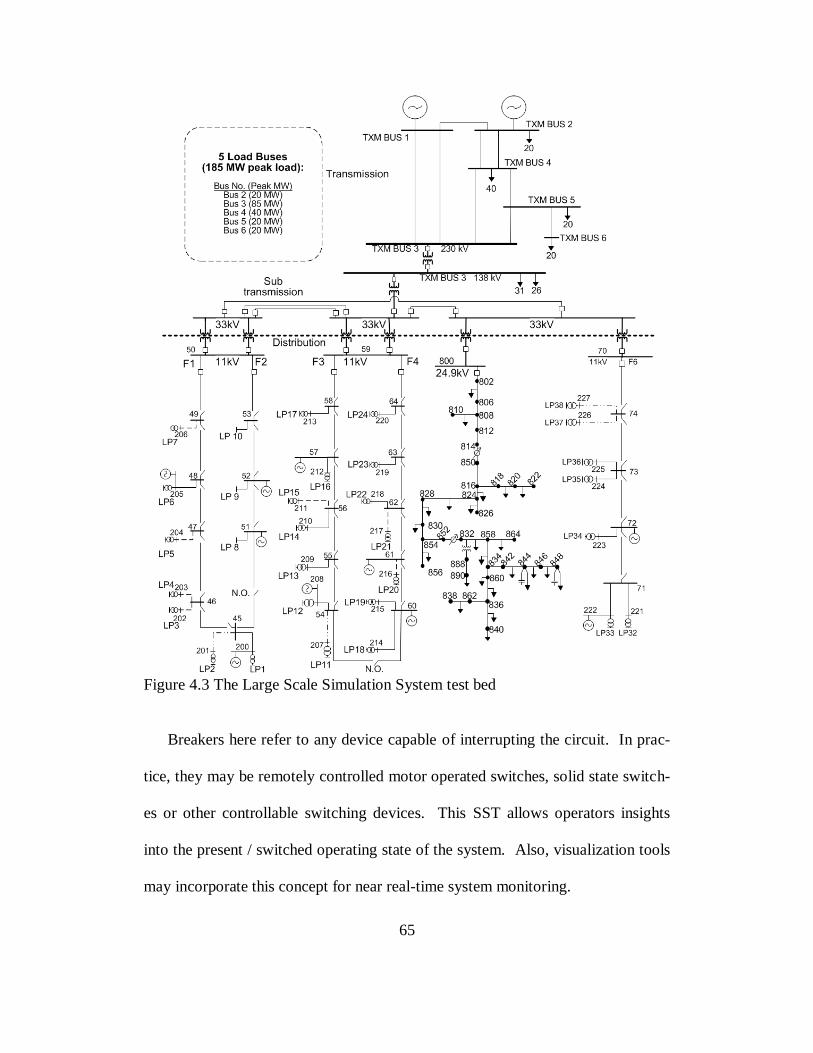
65
Figure 4.3 The Large Scale Simulation System test bed
Breakers here refer to any device capable of interrupting the circuit. In prac-
tice, they may be remotely controlled motor operated switches, solid state switch-
es or other controllable switching devices. This SST allows operators insights
into the present / switched operating state of the system. Also, visualization tools
may incorporate this concept for near real-time system monitoring.

66
The following example uses the system presented in Figure 4.1 to illustrate an
application in circuit design. The B matrix based algorithm may be used for real-
time monitoring of the distribution system and to trace circuit connectivity as
shown in Figure 2.5, Figure 2.6 and Figure 2.8 in Chapter 2. The objective of this
specific study is to maximize the load restored, and minimize unserved energy
following fault isolation. Practical implementations of this example may utilize a
centralized controller that monitors the distribution system in real-time and opti-
mizes automated circuit reconfiguration to meet preselected criteria.
4.6 Interrupting device location
To illustrate a circuit design application, tie switches in the RYG test bed of
Figure 4.1 were assumed to have remote operation ability, like a solid state switch
or breaker. Additional breakers (or switches) were added, one at a time, at vari-
ous locations in the test system. Adding interrupting devices changes the struc-
ture of the B matrix. Assuming that the probability of a fault is directly correlated
to the line length (i.e. longer lines are expected to experience faults more fre-
quently), pseudorandom fault locations were simulated on the distribution feeders.
This method is similar to the use of Monte Carlo simulation for evaluating power
system reliability [39].
Circuit connectivity is assessed following the locating of this pseudo-random
fault occurrence. Circuit reconfiguration and restoration options after isolating
the faulted subsystem is assessed through the tracing of connectivity using the B
matrix as identified in subsection 2.6 and using a system status table. The reduc-

67
tion in expectation of unserved energy after fault isolation is considered in adding
each additional breaker. Starting with four interrupting devices, one additional
breaker is added to the system. When the breaker location has been determined,
another breaker is added to the system, until a total of eight interrupting devices
are included.
The next interrupting device is added in the system on a line that does not al-
ready have an interrupting device (or switch) and the simulation is repeated as the
distribution system is stressed by faults. An optimal interrupting device location
allows isolation of faulted lines that have the greatest impact on expectation of
unserved energy following reconfiguration after fault isolation. The result ob-
tained is suboptimal for the following reasons: first, the bus loads are assumed to
be fixed; power flow limitations are not considered; and the location of n circuit
interrupting devices in m lines can occur according to the binomial coefficient
equation as follows,
.
According to this calculation, there are 1820 ways for which 4 interrupting devic-
es may be placed in 16 lines on this system. Only a small subset of the entire so-
lution set is simulated since for each interrupting device added to the system, a
minimum expectation of unserved energy is obtained. That is, a sequential ap-
proach to locating a breaker then calculating expectation of unserved energy is
used. Figure 4.4 shows how the expectation of unserved energy decreases as the
number of interrupting devices increases. Table 4.2 shows the result of calculated

68
expected unserved energy after four interrupting devices have been placed. Un-
served load refers to the average load that cannot be restored after 5000 pseudo-
randomly simulated faults on the system are isolated by circuit reconfiguration.
Table 4.2 Results of the Breaker Placement Algorithm
Breaker placed in line E(U) MWh
2, 3, 6, 17 1.2
4.7 Reconfiguration and restoration
For each available interrupting device combination, the B matrix algorithm is
used to find the total load connected to the substation buses. Once the fault has
been isolated, the status of interrupting devices is established. Note that there are
possible interrupting device configurations (where ncb is the number of
interrupting devices and m denotes interrupting devices that must remain open to
isolate faulted sections) allowable; there are
remaining configuration
states in the SST. An optimum solution selected as the resulting interrupting de-
vice combination that provides for the maximum load to be restored after the fault
is isolated by circuit reconfiguration. This is the target ‘optimum’ operating state
shown in Figure 2.5.
In an illustrative example, faults are once again pseudo-randomly located on
the system of Figure 4.1 to test the performance of the algorithm. With every
simulation, a feasible state is found, and at least one solution provides a maximum
value for load served. Most often, there are multiple solutions (multiple rows in
the SST) that correspond to the same value for maximum load restored; a prioriti-

69
zation method may be chosen so minimum switching operations are performed.
For instance, a permanent fault occurring in line 17 requires opening of interrupt-
ing devices in lines 17, and 18. Note that there are 28-2
= 64 possible interrupting
device configurations available since 2 of the 8 interrupting devices have been
locked out. Only a small subset of these possible configurations, however, will
allow the maximum load identified to remain energized. One possible interrupt-
ing device configuration (reconfiguration) that allows maximum load to be re-
stored after this fault isolation is given by the following:
close interrupting device T2
open interrupting devices in lines 17 and 18 (T3).
Under the stated conditions, a total load of 8 + j3.9 MVA is restored. Only load
connected to buses 18 and 19 (1 + j0.5 MVA) experiences an outage.
Figure 4.4 Expectation of unserved energy vs. no. of interruption devices RYG

70
4.8 Reliability enhancement and switching automation on the RBTS
For the application of the B matrix to the RBTS test bed, the previous ap-
proach of including interrupting devices one at a time was determined to be im-
practical for the demonstration of automated interrupting device location, since
there are a large amount of switches. Note that this applies for a high number of
automated isolation switches. Instead, cases were developed to assess the per-
formance of contemporary design, with a source breaker and normally open tie
switches, partial networking, and fully networked (parallel feeders only) distribu-
tion systems. Along with the placement of interrupting devices, manual switching
versus automation is also studied. Seven cases were examined for the RBTS test
bed. These seven cases are described in Table 4.3.
Table 4.3 Seven Cases for RBTS Reliability and Automation Illustrations
Case
No. Interrupting devices and location
Manual or
Automated
(M, A)
RBTS-1 Substation circuit breaker; normally open tie switch M, A
RBTS-2 Add one switch per feeder, located at the midpoint M
RBTS-3 Add one switch per feeder, located at the midpoint A
RBTS-4 One switch per lateral bus, located at source side M
RBTS-5 One switch per lateral bus, located at source side A
RBTS-6 Two switches per bus serving a lateral M
RBTS-7 Two switches on each bus serving a lateral A
For each of the cases presented, note that there is a manual switching and au-
tomated switching comparison for each switching configuration (conventional,
partial and fully networked). Note also that Case C6 data corresponds to the origi-

71
nal RBTS data as presented in [38]. The results are shown in Figures 4.4 and 4.5
with the reduction in expectation of unserved energy and the reduction in ex-
pected SAIDI on the circuit. Note that adding a few interrupting devices has the
biggest immediate impact on reducing SAIDI. Furthermore, automation has the
potential to increase reliability over manual (time-consuming) switching. Cost is
generally a limiting factor in automation and control of the distribution infrastruc-
ture.
It is important in many automated systems that controls exist such that an op-
erator may assume control of the distribution system. For example, maintenance
work or construction may require that automated system reconfiguration or resto-
ration be disengaged for the safety of utility personnel or construction workers.
The RBTS system of Figure 4.2 depicts the distribution network of bus 3 with
44 load buses, 77 line segments, switches and normally open points. In this illus-
tration, examples compare the reliability enhancement of replacing manually op-
erated isolation switches with remotely controlled switches in selected locations.
This example assumes FDIR systems operate in an ideal manner and switching
does not necessarily replace protection systems (i.e. protection systems clear
faults, then reconfiguration may be undertaken post fault-clearing).
In this example, switching times are drastically reduced for automated restora-
tion and system reconfiguration scenarios; that is, switching times in automated
systems may be under 5 minutes so as to influence SAIDI and SAIFI indices.
Failure probability and frequency of events are held constant for comparison pur-

72
poses. The results obtained show that average repair times, annual unavailability
and expectation of unserved energy can be reduced.
Figure 4.5 Expectation of unserved energy vs. no. of interruption devices RBTS
Figure 4.6 SAIDI versus number of interruption devices RBTS
Table 4.4 presents load point reliability indices of the base case situation pre-
sented in reference [38]. Table 4.5 presents results of an automated, ‘smart’ dis-

73
tribution system. As indicated, λ values for each load point are the same in each
case, but all other indices are reduced with automation. Both tables 4.5 and 4.6
present failure rate (λ), repair time (r), annual unavailability (U) and expectation
of unserved energy (E). Table 4.4 data is presented in reference [38] and serves as
the benchmar by which ‘upgrades’ to the distribution system depicted in Figure
4.2 may be compared.
With the assumption that all switches in all feeders can be made remotely con-
trollable and automated to switch within a 5 second time frame, the resulting reli-
ability improvements to the system were calculated. These calculated improve-
ments in load point (bus) reliability indices identified in [38] and system wide re-
liability indices are presented in Table 4.5. Note that SAIDI falls by almost 7.0%,
while SAIFI remains the same. That is, with the same anticipated number of
events, the duration of events can be drastically reduced by automated reconfigu-
ration. Note also that the total expectation of unserved energy reduces by 14.3%.
Reference [117] goes on to estimate costs of reliability improvement by using
historical price information and categorizing loads according to size and type.
Note that all load size, classification and other pertinent data are provided in ref-
erences [29]-[31], [37]-[40]. It should be noted here that further networking of the
primary distribution system, and especially of the secondary distribution system,
can produce far greater reductions in r, U, E, and SAIDI, as reliability increases
when the number of redundant paths increase.

74
Table 4.4 Base Case Reliability Indices for Bus 3 of the RBTS System Load Point λ (f/y) r (h) U (h/y) E (MWh/y)
1 0.3010 11.4352 3.4420 1.6122 3 0.3140 11.1688 3.5070 1.0121 8 0.2210 1.9412 0.4290 0.3634
27 0.3205 10.9626 3.5135 1.9957 41 0.1885 1.8276 0.3445 2.5319 44 0.2015 1.7742 0.3575 1.5689
Total† 66.68
SAIDI 3.4726 SAIFI 0.3028
* The data in the table are taken directly from [38] and they do not entail the use of any electronic
switching devices. The notation f/y refers to failures per year. † The total energy unserved is summed over all 44 load points
Table 4.5 Reliability Indices for Bus 3 of the RBTS with Electronic Switching Load Point λ (f/y) r (h) U (h/y) E (MWh/y)
1 0.3010 10.6146 3.1950 1.4965 3 0.3140 10.3822 3.2600 0.9408 8 0.2210 1.1765 0.2600 0.2203
27 0.3205 10.1716 3.2600 1.8517 41 0.1885 1.0345 0.1950 1.4332 44 0.2015 0.9678 0.1950 0.8558
Total† 57.14
SAIDI 3.2322 SAIFI 0.3028
*The data in the table reflect system performance with electronic devices inserted in every branch.
Note the improvement over data shown in [38] (Table 4.4). † The total energy unserved is summed over all 44 load points
4.9 Discussion of reliability enhancement and restoration examples
The preceding examples demonstrated new algorithms, applications and con-
trol options for the smart distribution system. Examples of algorithms for use in
distribution system reliability enhancement and restoration were presented. The
effect of automation in switching and restoration functions was shown, and relat-
ed distribution system reliability indices were used to quantify expected im-
provements in reliability.

75
On the RYG test bed, breakers were located such that expectation of unserved
energy following disturbances in the distribution system is minimized. By adding
four breakers to the system, expectation of unserved energy was reduced from
2.85 MWh/yr to approximately 1.15 MWh/yr.
Studies on the RBTS test bed showed reliability improvements via increasing
the number of interrupting devices, and by automating restoration / switching in
the distribution system. The results show that feeder automation and enhance-
ment of network reconfiguration options may have a significant effect on improv-
ing expected reliability for similar expected failure rates. SAIDI was shown to
reduce by 7 % by fully automating restoration. Expectation of unserved energy
was shown to reduce by 14 % by fully automating switching and restoration.
Limitations within examples shown include the omission of cost-benefit evalua-
tion for practical implementation.

76
5. Illustrations of three-phase distribution system state estimation
5.1 Distribution system state estimation
All illustrations of the three-phase distribution system state estimation algo-
rithm are shown for feeder F1 of the RBTS Bus 3 distribution sub-network, which
has been developed in three-phase detail and is shown in Figure 5.1. Loading
conditions for the illustrations are described in this subsection and additional data
is provided in 0.
Figure 5.1 Three-phase detail of RBTS feeder F1
Table 5.1 Examples Presented in Chapter 5
RBTS Feeder
F1 (3ϕ) circuit Examples
Distribution class state estimator x SE1, SE2, SE3
Weighted estimation x SE1, SE2, SE3
Bad data detection x SE2
As discussed in Chapters 1-4, the factors influencing the evolution of distribu-
tion systems also necessitate new tools for enhancing monitoring, operations and
control. Distribution class state estimation has the potential to allow increased

77
levels of automation, control and to enhance operator interface. Of particular in-
terest are those distribution networks with the following characteristics: high pen-
etration of distributed generation; ability to selectively network to change power
flows, voltage profiles and reduce losses; inclusion of new voltage regulation
tools such as series and shunt capacitors and reactors.
To enable state estimation applications, sufficient measurement capabilities
are needed. Measurements are envisioned with existing technology such as smart
meters and conventional voltage magnitude, current magnitude and real and reac-
tive power flow meters. Future generations of measurement devices are envi-
sioned to have the capability to capture completely synchronized phasor quanti-
ties. Note that even conventional smart meters may be synchronized, but not to
the level of detail to capture phasor quantities.
A key aspect of distribution system state estimation is the intended end-goal.
It may be argued that the highly stochastic nature of distribution system loads
(and renewable electric generation in distribution systems) makes fast re-
sponse/control to rapid (seconds) changes impractical. However, enabling control
as a response to ‘slower’ system changes (i.e. feeder loading / unloading and volt-
age unbalance over a day), or large fluctuations (i.e. sustained sudden shifts in
power flows or voltage magnitudes) appears to be a feasible enhancement to dis-
tribution control. Examples of applications that are enabled through the use of
state estimation include:

78
As indicated in [85], DGs may be blocked from connecting to the grid if
voltages exceed specified ranges. To maximize effective use of DG as-
sets, utilities may need additional voltage regulation resources that in-
crease operating flexibility in the distribution system.
DG may potentially increase voltage unbalance between phases. Three-
phase motors are sensitive to small voltage unbalance. Utilities may also
require voltage balancing mechanisms beyond traditional regulators (that
regulate each phase separately).
Demand response and direct load control needs to be accomplished in a
manner that does not exacerbate voltage unbalance or otherwise negative-
ly impact system operations.
Monitoring of line flows, transformer loading, and bus voltage magnitudes
provide operators increased insights into the system. Operators may avert
potential unsafe conditions with adequate visualization options and alerts
to potential overloads.
Knowledge of pre-outage loading may enhance restoration practice, espe-
cially for short duration outages.
The following illustration demonstrates the use of a distribution class estima-
tor to calculate system states based on assumed system measurements. The true
solution to the network is assumed to be the results of a power flow study based
on a known load (i.e. ladder iterative or other). Those bus voltage magnitudes
and angles obtained from the power flow solution are exact for the specific oper-
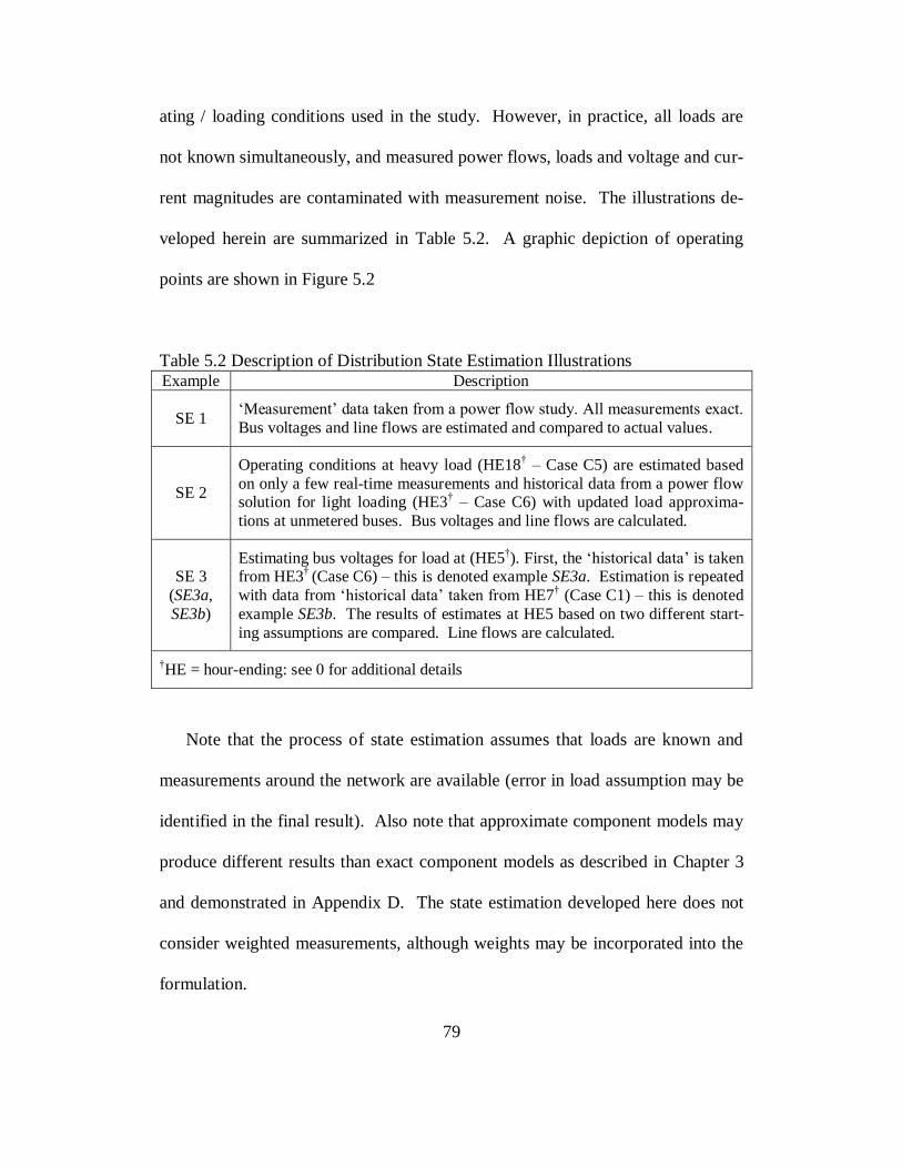
79
ating / loading conditions used in the study. However, in practice, all loads are
not known simultaneously, and measured power flows, loads and voltage and cur-
rent magnitudes are contaminated with measurement noise. The illustrations de-
veloped herein are summarized in Table 5.2. A graphic depiction of operating
points are shown in Figure 5.2
Table 5.2 Description of Distribution State Estimation Illustrations Example Description
SE 1 ‘Measurement’ data ta en from a power flow study. All measurements exact.
Bus voltages and line flows are estimated and compared to actual values.
SE 2
Operating conditions at heavy load (HE18† – Case C5) are estimated based
on only a few real-time measurements and historical data from a power flow solution for light loading (HE3
† – Case C6) with updated load approxima-
tions at unmetered buses. Bus voltages and line flows are calculated.
SE 3 (SE3a,
SE3b)
Estimating bus voltages for load at (HE5†). First, the ‘historical data’ is taken
from HE3†
(Case C6) – this is denoted example SE3a. Estimation is repeated
with data from ‘historical data’ ta en from HE7† (Case C1) – this is denoted
example SE3b. The results of estimates at HE5 based on two different start-
ing assumptions are compared. Line flows are calculated.
†HE = hour-ending: see 0 for additional details
Note that the process of state estimation assumes that loads are known and
measurements around the network are available (error in load assumption may be
identified in the final result). Also note that approximate component models may
produce different results than exact component models as described in Chapter 3
and demonstrated in Appendix D. The state estimation developed here does not
consider weighted measurements, although weights may be incorporated into the
formulation.

80
Figure 5.2 Graphic of operating points for HE3, HE5, HE7 and HE18.
The Cooper Power Systems software package, CYMDIST, was used to obtain
solved power flow solutions for the RBTS network. A Matlab ladder iterative
solver was also developed for this study. The resulting voltage profiles obtained
from ladder iterative solutions in CYMDIST and Matlab agree exactly. Table 5.3
provides a summary of the 7 distinct cases studied, and Table 5.4 provides load-
ing conditions as seen by the substation transformer.
Note that the seven cases are just a sampling of the 24 hour load profile as
seen by the distribution substation transformer of feeder F1 shown in Figure 5.1.
Each case corresponds to a different feeder loading condition as detailed explicit-
ly in 0. The system base for all measurements and per-unit impedances is 100
MVA3ϕ.

81
Table 5.3 RBTS Feeder F1 Loading Conditions Considered for SE Examples
Lo
ad
(Cas
e)
Des
crip
-
tio
n
Ph
ase
Load served at bus (MVA)
LP1 LP 2 LP 3 LP 4 LP 5 LP 6 LP 7
C1 Base
case
(HE7)
A 0.2789 0.2583 - - - 0.2789 0.2789
B 0.2789 0.2583 - 0.2789 - 0.2789 -
C 0.2789 - 0.1741 - 0.2789 0.2789 -
HE5 Between
C6 – C1
A 0.200
+j0.040
0.250
+j0.060 - - -
0.230
+j0.060
0.150
+j0.0450
B 0.200
+j0.045
0.250
+j0.065 -
0.200
+j0.040 -
0.205
+j0.055 -
C 0.200
+j0.040 -
0.155
+j0.030 -
0.2000
+j0.050
0.230
+j0.060 -
C2 Heavy
load 1
(HE12)
A 0.2789
+j0.150
0.2583
+j0.140 - - -
0.2789
+j0.150
0.350
+j0.180
B 0.2789
+j0.150
0.2583
+j0.140 -
0.2789
+j0.155 -
0.500
+j0.200 -
C 0.2789
+j0.150 -
0.274
+j0.140 -
0.2789
+j0.150
0.2789
+j0.150 -
C3 Heavy
load 2
(HE16)
A 0.3789 +j0.20
0.3583 +j0.195
- - - 0.3789 +j0.200
0.350 +j0.180
B 0.3789
+j0.200
0.2583
+j0.140 -
0.3100
+j0.170 -
0.500
+j0.270 -
C 0.3789
+j0.200 -
0.305
+j0.160 -
0.320
+j0.200
0.350
+j0.20 -
C4 Heavy load 2 with capacitor at bus 48. Loads are the same as Case C3 .
C5
Heavy
load 3
(HE18
peak)
A 0.470
+j0.220
0.470
+j0.230 - - -
0.450
+j0.240
0.4500
+j0.220
B 0.450
+j0.200
0.490
+j0.250 -
0.450
+j0.218 -
0.510
+j0.250 -
C 0.390
+j0.150 -
0.450
+j0.230 -
0.450
+j0.218
0.450
+j0.20 -
C6 Light
Load
(HE3)
A 0.0925
+j0.033
0.150
+j0.035 - - -
0.1175
+j0.036
0.1025
+j0.033
B 0.1000
+j0.030
0.1625
+j0.038 -
0.0925
+j0.032 -
0.1275
+j0.038 -
C 0.0975 +j0.023
- 0.100
+j0.035 -
0.125 +j0.037
0.1125 +j0.030
-
Figures showing main feeder and load point voltage magnitudes from power
flow solutions are presented. Figure 5.3 - Figure 5.5 show bus voltage magni-
tudes along the three-phase main feeder (buses 45–50) and bus voltage magnitude
at the load (buses 1–7). Data used to construct these figures are provided in tables
in 0 and Appendix D.

82
Table 5.4 Feeder Load as Seen by the Substation Transformer for Each Case
Load Case
Load seen from the substation (MVA) MW Total
MVAr Total
Substation Load
(MVA) Phase A Phase B Phase C
HE7 - C1 1.11 1.11 1.03 3.20 0.60 3.26
HE12 - C2 1.32 1.47 1.26 3.59 1.86 4.04
HE16 - C3 1.66 1.64 1.55 4.27 2.32 4.85
HE16 - C4 1.66 1.64 1.55 4.27 2.32 4.85
HE18 - C5 2.05 2.11 1.91 5.48 2.63 6.08
HE3 - C6 0.48 0.50 0.45 1.38 0.39 1.43
HE5 0.86 0.88 0.805 2.47 0.59 2.54
The process matrix, h, contains measurement data, pseudo-measurements and
other pertinent topological data. Note that pseudo-measurements may be based
on historical data, reasonable assumptions (i.e. voltage magnitudes of 1.0 p.u.,
angles in phases a, b, c of 0, 240, 120 degrees respectively) of unmeasured quanti-
ties and previously obtained network solutions.
Pseudo-measurements are also used in transmission system state estimation
formulations. Pseudo-measurements are derived from the solution to a distribu-
tion power flow (i.e. ladder iterative or other procedure). The forward / backward
sweep method incorporates load and topology assumptions and provides a feasi-
ble solution to the network. The linearized state estimation formulation incorpo-
rates real-time measured, pseudo-measurements and calculations / assumptions
for unmeasured loads.
The flow chart of Figure 5.6 outlines this concept. The state vector is taken as
the three-phase real and imaginary part of voltage. In the examples developed
here, real and reactive power measurements are converted to equivalent currents
to be incorporated into the state estimation,

83
(5.1)
U = identity matrix
hLM = line measurement coefficient matrix
YBUS = system admittance model
Vmeas, Imeas, Iline measurement vectors
Imeas contains measured and assumed injections / loads
Note that injection current ‘measurements’ include those measurements from
transducers as well as those pseudo-measurements obtained from historical (i.e.
power flow solution). The corresponding line currents are calculated from the
estimated voltages. Line current magnitudes on the main feeder are shown in Fig-
ure 5.9. Error in line current phase angle is shown in Figure 5.10. Note that line
currents obtained from the estimator are nearly identical to power flow results (i.e.
bus voltages are identical). In the subsequent examples, measurement devices
(smart meters or synchronized phasor devices) are assumed to be located at load
buses 2, 5, and 6, and on main feeder buses / transformer primary buses 11, 14,
45, 46 and 48 respectively.
Approximating non-measured load values
The smart distribution infrastructure is likely to have widely deployed smart
metering. However, not every load point may be measured. Reasonable approxi-
mations of non-measured load values are made. Approximations are made based

84
on substation injection and measured loads. Bus voltage phase angles are deter-
mined as follows: available from synchrophasors, approximated from power flow
data (pseudo), or assigned because the bus is close to a synchrophasor.
Bus voltage magnitude and aggregate load active and reactive power meas-
urements are available at buses 2, 5, 6. Synchrophasor voltage measurements are
assumed at buses 11, 14 distribution transformer primary, and main feeder buses
45, 46, and 48. At load points where no measurement devices are present (aggre-
gate load unknown), an algorithm is used to apportion the unmeasured load based
on historical loading and reasonable assumptions at the load point. Power flows
measured at the substation,
Psub = + Plosses (5.2)
where n is the number of buses, and Plosses may be unknown or approximate.
Measured bus loads total,
Pmeas = Pl (5.3)
where k is the number of measured load points. When substation active power
flow changes are observed,
ΔPsub = + ΔPlosses (5.4)
Aggregate unmeasured demands are approximated via,
Punmeas + Plosses = Psub – Pmeas (5.5)
Then, when substation power flow and measured loads change, the corresponding
change in unmeasured aggregate load and subsequently unmeasured individual
loads (historical or assumed) may be approximated,

85
ΔPunmeas = ΔPsub - ΔPmeas (5.6)
ΔPi_unmeas = Pi_unmeas
(5.7)
Limitations and weights based on historical data or installed capacity may be
imposed. However, care must be taken in limiting load estimation due to the high-
ly stochastic nature of the individual instantaneous load. In the longer time hori-
zon, load growth may need to be considered. Reactive power assumptions also
follow (15)-(20), and total feeder power factor change can be used to check accu-
racy of assumptions.
Table 5.5 Demand at Each Bus Used in SE3a, SE3b, and SE2
Demand at each bus (P/ Q in kW/ kVAr)
1† 2 3
† 4
† 5 6 7
†
Power
flow 600/ 125 500/ 125 155/ 30 200/ 40 200/ 50 665/ 175 150/ 45
SE3a,
SE2 549/ 111 607/ 95 180/ 42 192/ 44 216/ 40 678/ 134 184/ 43
SE3b 594/ 116 347/ 125 136/ 39 200/ 40 219/ 39 594/ 162 175/ 45 † Pseudomeasurement – demand calculated based on measurements at other buses and the
substation according to (15)-(20). Metered (measured) values are shown in shaded columns.
Example SE1
Table 5.6 presents the true solution as obtained from a ladder iterative power
flow study for the 20 (three-phase) buses in the RBTS feeder F1 network base
case – Case C1. Table 5.7 presents the resulting branch currents for Case C1.
The non-iterative, linear estimation utilizes ‘measured’ data at buses 2, 5, 6, ,
14, 45, 46, 48.

86
Figure 5.3 Phase A bus voltage magnitudes (a) along the main feeder and (b) at
load buses, cases C1-C6
Figure 5.4 Phase B bus voltage magnitudes (a) along the main feeder and (b) at
load buses, cases C1-C6
Figure 5.5 Phase C bus voltage magnitudes (a) along the main feeder and (b) at
load buses, cases C1-C6

87
Figure 5.6 Flowchart of the distribution system state estimation algorithm

88
Table 5.6 Bus Voltages from a Power Flow Study for HE7 Loading Condition,
Case C1, RBTS Feeder F1, Figure 5.1
Bus No. |Va|
(p.u.)
Angle Va
(deg.)
|Vb|
(p.u.)
Angle Vb
(deg.)
|Vc|
(p.u.)
Angle Vc
(deg.)
50 1.0000 0.00 1.0000 -120.00 1.0000 120.00
49 0.9968 -0.24 0.9977 -120.22 0.9988 119.80
48 0.9933 -0.44 0.9926 -120.57 0.9979 119.44
47 0.9913 -0.53 0.9888 -120.81 0.9977 119.19
46 0.9880 -0.64 0.9855 -121.15 0.9986 119.03
45 0.9857 -0.77 0.9848 -121.31 0.9989 119.01
14 0.9959 -0.36
13 0.9923 -0.51 0.9918 -120.63 0.9975 119.37
12 0.9969 119.11
11 0.9842 -121.33
10 0.9974 118.89
9 0.9841 -0.83 0.9848 -121.41
8 0.9850 -0.84 0.9841 -121.37 0.9986 118.94
7 0.9944 -0.89
6 0.9903 -1.01 0.9899 -121.13 0.9954 118.90
5 0.9952 118.73
4 0.9828 -121.87
3 0.9957 118.41
2 0.9820 -1.34 0.9826 -121.92
1 0.9836 -1.43 0.9825 -121.96 0.9972 118.37
Table 5.7 Line Currents from Power Flow Study for HE7 Loading Condition,
Case C1, RBTS Feeder F1, Figure 5.1 From bus
To bus
|Ia| (Amps)
Angle Ia (deg.)
|Ib| (Amps)
Angle Ib (deg.)
|Ic| (Amps)
Angle Ic (deg.)
49 50 177.64 -11.78 178.21 -132.33 161.42 107.29
48 49 133.54 -12.31 178.21 -132.33 161.42 107.29
47 48 91.14 -11.51 135.94 -132.10 120.78 107.92
46 47 91.14 -11.51 135.94 -132.10 88.24 109.11
45 46 91.14 -11.51 91.46 -133.05 47.79 110.78
14 49 44.13 -10.18
13 48 42.43 -14.01 42.27 -133.08 40.67 105.40
12 47
32.62 104.69
11 46
44.52 -130.14
10 46
40.49 107.15
9 45 42.78 -14.34 42.95 -135.95
8 45 48.45 -9.02 48.61 -130.49 47.79 110.78
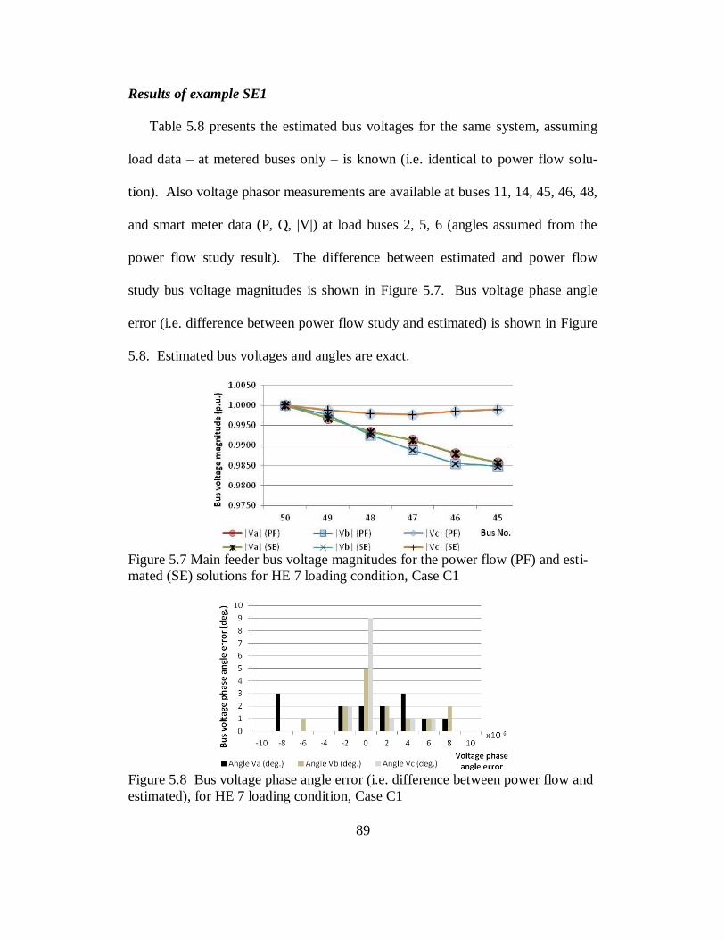
89
Results of example SE1
Table 5.8 presents the estimated bus voltages for the same system, assuming
load data – at metered buses only – is known (i.e. identical to power flow solu-
tion). Also voltage phasor measurements are available at buses 11, 14, 45, 46, 48,
and smart meter data (P, Q, |V|) at load buses 2, 5, 6 (angles assumed from the
power flow study result). The difference between estimated and power flow
study bus voltage magnitudes is shown in Figure 5.7. Bus voltage phase angle
error (i.e. difference between power flow study and estimated) is shown in Figure
5.8. Estimated bus voltages and angles are exact.
Figure 5.7 Main feeder bus voltage magnitudes for the power flow (PF) and esti-
mated (SE) solutions for HE 7 loading condition, Case C1
Figure 5.8 Bus voltage phase angle error (i.e. difference between power flow and
estimated), for HE 7 loading condition, Case C1

90
Table 5.8 Estimated Bus Voltages, RBTS Feeder F1, Figure 5.1–Case C1
Case C1 - Base Case Voltage measurements: [2 5 6 11 14 45 46 48]
Bus No.
|Va| (p.u.)
Angle Va (deg.)
|Vb| (p.u.)
Angle Vb (deg.)
|Vc| (p.u.)
Angle Vc (deg.)
50 1.0000 0.00 1.0000 -120.00 1.0000 120.00
49 0.9968 -0.24 0.9977 -120.22 0.9988 119.80
48 0.9933 -0.44 0.9926 -120.57 0.9979 119.44
47 0.9913 -0.53 0.9888 -120.81 0.9977 119.19
46 0.9880 -0.64 0.9855 -121.15 0.9986 119.03
45 0.9857 -0.77 0.9848 -121.31 0.9989 119.01
14 0.9959 -0.36
13 0.9923 -0.51 0.9918 -120.63 0.9975 119.37
12
0.9969 119.11
11
0.9842 -121.33
10
0.9974 118.89
9 0.9841 -0.83 0.9848 -121.41
8 0.9850 -0.84 0.9841 -121.37 0.9986 118.94
7 0.9944 -0.89 6 0.9903 -1.01 0.9899 -121.13 0.9954 118.90
5 0.9952 118.73
4 0.9828 -121.87
3 0.9957 118.41
2 0.9820 -1.34 0.9826 -121.92
1 0.9836 -1.43 0.9825 -121.96 0.9972 118.37
Figure 5.9 Main feeder line current magnitudes from power flow (PF) and esti-
mated (SE), for HE7 loading condition, Case C1

91
Figure 5.10 Difference between current magnitudes for the power flow and esti-
mated solution corresponding to HE 7 loading condition, Case C1
Figure 5.11 Current phase angle error histogram (i.e. difference between power
flow and estimated solution), for HE7 loading condition, Case C1
Example SE2
Example SE2 estimates bus voltages at peak load (HE18 – Case C5). It is as-
sumed that individual loads were known at a light load condition (HE3 – Case
C6) for which a power flow study result is available. Note that at some instant in
HE18, bus voltages are measured in full phasor detail at transformer primary bus-

92
es 11, 14 and at main feeder buses 45, 46 and 48. Bus voltage magnitudes at bus-
es 2, 5, and 6 are also available. Power flowing into the circuit at the substation is
measured. Loads at buses 2, 5 and 6 are also measured. The different states are
depicted in Figure 5.2. The unknown load values are assumed (scaled based on
known values at HE3 to match substation flow at HE18). The state vector at
HE18 is then estimated.
Table 5.9 and Table 5.10 present bus voltages obtained from the power flow
study of RBTS feeder F1 as depicted in Figure 5.1 for HE3 (Case C6) and HE18
(Case C5) respectively. Table 5.11 presents line currents on the main feeder and
two laterals farthest from the substation for both cases (light load at HE3 and peak
load at HE18).
Results of example SE2
The resulting state estimates are shown in the subsequent figures. Figure 5.12
shows main feeder bus voltage magnitudes for both the estimated and actual
(power flow) solutions. Figure 5.13 presents the error histograms depicting num-
ber of bus within an error range (i.e. difference between the power flow study and
estimated solutions). Figure 5.14 shows voltage phase angle error between power
flow and estimated results.

93
Table 5.9 Bus Voltages from a Power Flow, RBTS Feeder F1, Figure 5.1–HE3,
Case C6
Bus No. |Va|
(p.u.) Angle Va
(deg.) |Vb|
(p.u.) Angle Vb
(deg.) |Vc|
(p.u.) Angle Vc
(deg.)
50 1.0000 0.00 1.0000 -120.00 1.0000 120.00
49 0.9984 -0.09 0.9988 -120.10 0.9995 119.91
48 0.9967 -0.17 0.9963 -120.25 0.9990 119.76
47 0.9958 -0.21 0.9945 -120.34 0.9987 119.65
46 0.9941 -0.25 0.9930 -120.49 0.9992 119.60
45 0.9928 -0.30 0.9927 -120.57 0.9995 119.61
14 0.9980 -0.13
13 0.9962 -0.20 0.9958 -120.28 0.9989 119.73
12
0.9983 119.60
11
0.9924 -120.55 10
0.9986 119.55
9 0.9918 -0.33 0.9927 -120.64 8 0.9925 -0.32 0.9924 -120.59 0.9994 119.59
7 0.9969 -0.33
6 0.9950 -0.42 0.9945 -120.53 0.9979 119.51
5
0.9972 119.38
4
0.9913 -120.72
3
0.9974 119.36
2 0.9907 -0.62 0.9914 -120.95
1 0.9914 -0.50 0.9914 -120.79 0.9987 119.41
Figure 5.12 Bus voltage magnitudes along main feeder RBTS feeder F1, Figure
5.1, for HE18 loading condition, power flow and estimated solution
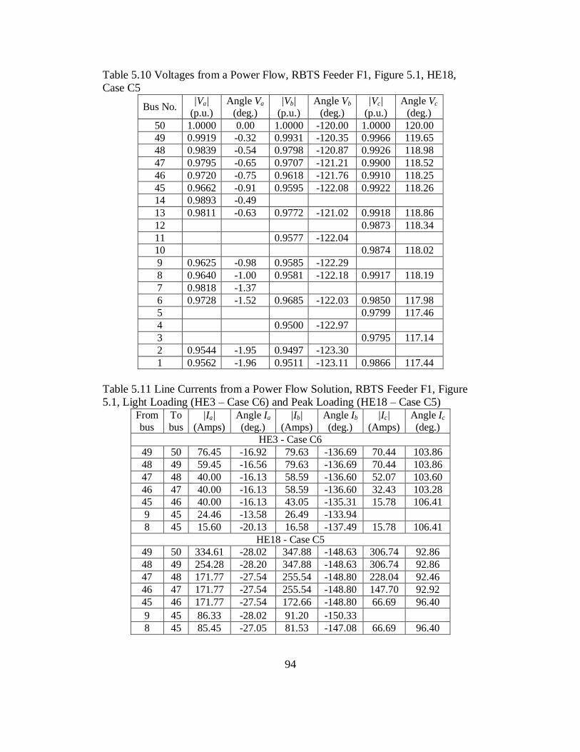
94
Table 5.10 Voltages from a Power Flow, RBTS Feeder F1, Figure 5.1, HE18,
Case C5
Bus No. |Va|
(p.u.) Angle Va
(deg.) |Vb|
(p.u.) Angle Vb
(deg.) |Vc|
(p.u.) Angle Vc
(deg.) 50 1.0000 0.00 1.0000 -120.00 1.0000 120.00 49 0.9919 -0.32 0.9931 -120.35 0.9966 119.65 48 0.9839 -0.54 0.9798 -120.87 0.9926 118.98 47 0.9795 -0.65 0.9707 -121.21 0.9900 118.52 46 0.9720 -0.75 0.9618 -121.76 0.9910 118.25 45 0.9662 -0.91 0.9595 -122.08 0.9922 118.26 14 0.9893 -0.49
13 0.9811 -0.63 0.9772 -121.02 0.9918 118.86 12
0.9873 118.34 11
0.9577 -122.04
10
0.9874 118.02 9 0.9625 -0.98 0.9585 -122.29
8 0.9640 -1.00 0.9581 -122.18 0.9917 118.19 7 0.9818 -1.37
6 0.9728 -1.52 0.9685 -122.03 0.9850 117.98 5
0.9799 117.46 4
0.9500 -122.97
3
0.9795 117.14 2 0.9544 -1.95 0.9497 -123.30
1 0.9562 -1.96 0.9511 -123.11 0.9866 117.44
Table 5.11 Line Currents from a Power Flow Solution, RBTS Feeder F1, Figure
5.1, Light Loading (HE3 – Case C6) and Peak Loading (HE18 – Case C5) From bus
To bus
|Ia| (Amps)
Angle Ia (deg.)
|Ib| (Amps)
Angle Ib (deg.)
|Ic| (Amps)
Angle Ic (deg.)
HE3 - Case C6 49 50 76.45 -16.92 79.63 -136.69 70.44 103.86 48 49 59.45 -16.56 79.63 -136.69 70.44 103.86 47 48 40.00 -16.13 58.59 -136.60 52.07 103.60 46 47 40.00 -16.13 58.59 -136.60 32.43 103.28 45 46 40.00 -16.13 43.05 -135.31 15.78 106.41 9 45 24.46 -13.58 26.49 -133.94
8 45 15.60 -20.13 16.58 -137.49 15.78 106.41 HE18 - Case C5
49 50 334.61 -28.02 347.88 -148.63 306.74 92.86 48 49 254.28 -28.20 347.88 -148.63 306.74 92.86 47 48 171.77 -27.54 255.54 -148.80 228.04 92.46 46 47 171.77 -27.54 255.54 -148.80 147.70 92.92 45 46 171.77 -27.54 172.66 -148.80 66.69 96.40
9 45 86.33 -28.02 91.20 -150.33 8 45 85.45 -27.05 81.53 -147.08 66.69 96.40

95
Figure 5.13 Voltage magnitude error histogram (i.e. difference between power
flow and estimated solution), example SE2
Figure 5.15 shows line current magnitudes along the main feeder for both the
power flow (true) and estimated solutions. Figure 5.16 and Figure 5.17 show er-
ror histograms for branch current magnitude and phase angle errors respectively.
Figure 5.14 Bus voltage phase angle error histogram (i.e. difference between
power flow study and estimated), example SE2

96
Figure 5.15 Line current magnitudes along the main feeder for RBTS feeder F1,
power flow and estimated
Figure 5.16 Branch current magnitude error (Amps), RBTS feeder F1, SE2
Figure 5.17 Branch current phase angle error (deg.), RBTS feeder F1, SE2

97
Example SE3
Example SE3 evaluates the estimator algorithm performance under a different
set of circumstances. The test bed RBTS feeder F1, in full three-phase detail, as
shown in Figure 5.1 is used. The system state under the loading conditions at
hour ending (HE) 5:00 is estimated from two different starting assumptions, de-
noted here as SE3a and SE3b. Loading condition at HE 5:00 is estimated, first
using the known (power flow) loads at HE3 (Case C6) – SE3a. The process is
repeated for the known loads at HE7 (Case C1). Loading conditions for the three
cases are as follows (details are shown graphically in Figure 5.2):
HE 3:00, Case C6, substation serves load of 1.43 MVA
HE 5:00, substation serves load of 2.54 MVA
HE 7:00, Case C1, substation serves load of 3.26 MVA.
Table 5.12 Values of Non-Metered (Pseudo-Measurement) Loads Obtained from
Equations (5.2) – (5.7) at HE5
Non-metered load at HE 5
Actual Based on HE 3 Based on HE 7 P (kW) Q (kVAr) P (kW) Q (kVAr) P (kW) Q (kVAr)
LP 1 600 125 549 111 594 116 LP 3 155 30 180 42 136 39 LP 4 200 40 192 44 200 40 LP 7 150 45 184 43 175 45
Bus voltage magnitudes during HE3 (Case C6) and HE7 (Case C1) have al-
ready been shown in Table 5.9 and Table 5.6 respectively. Line current magni-
tudes for both loading conditions have also been presented in Table 5.7 and Table
5.11. Voltage magnitudes from the power flow study results for HE5 loading is
shown in Table 5.13. Line currents for HE5 solution is shown in Table 5.14. The

98
specific loads at HE5 are largely unknown to the estimator (only measured bus
values are known).
Note that bus voltages at buses 2, 5, 6, 11, 14, 45, 46, and 48 are measured,
and are updated in the state estimation stage of the algorithm. Also, bus voltage
and power flowing into the circuit from the substation is known. Estimating
states under HE 5 (05:00) loading conditions is first performed based on the pow-
er flow results of HE 3 (03:00). The estimation process is repeated, however, the
‘most recent’ power flow study results of HE 7 (7:00) are used to supplement
non-measured data.
Table 5.13 Bus Voltages from a Power Flow Study, RBTS Feeder F1 for Loading
Condition HE5 Bus No.
|Va| (p.u.)
Angle Va (deg.)
|Vb| (p.u.)
Angle Vb (deg.)
|Vc| (p.u.)
Angle Vc (deg.)
50 1.0000 0.00 1.0000 -120.00 1.0000 120.00
49 0.9974 -0.17 0.9979 -120.17 0.9991 119.84
48 0.9944 -0.34 0.9938 -120.44 0.9983 119.56
47 0.9925 -0.41 0.9909 -120.63 0.9981 119.38
46 0.9895 -0.50 0.9884 -120.91 0.9991 119.30
45 0.9874 -0.61 0.9878 -121.04 0.9995 119.30
14 0.9967 -0.23 13 0.9936 -0.41 0.9931 -120.48 0.9976 119.49
12
0.9973 119.30
11
0.9873 -121.03
10
0.9984 119.21
9 0.9858 -0.66 0.9878 -121.14
8 0.9868 -0.65 0.9873 -121.08 0.9992 119.26
7 0.9952 -0.52
6 0.9915 -0.85 0.9913 -120.87 0.9956 119.05
5
0.9956 118.92
4
0.9859 -121.42 3
0.9974 118.92
2 0.9838 -1.15 0.9856 -121.62 1 0.9855 -1.04 0.9858 -121.47 0.9979 118.88

99
Table 5.14 Line Currents Obtained from a Power Flow Study, RBTS Feeder F1,
Figure 5.1, HE 5 From bus
To bus
|Ia| (Amps)
Angle Ia (deg.)
|Ib| (Amps)
Angle Ib (deg.)
|Ic| (Amps)
Angle Ic (deg.)
49 50 136.21 -14.79 140.26 -134.84 127.26 106.03
48 49 111.46 -14.25 140.26 -134.84 127.26 106.03
47 48 73.72 -13.63 106.55 -134.51 89.68 106.70
46 47 73.72 -13.63 106.55 -134.51 57.11 107.74
45 46 73.72 -13.63 74.00 -135.29 32.18 107.57
14 49 24.78 -17.22
13 48 37.75 -15.47 33.71 -135.89 37.59 104.43
12 47
32.60 104.88
11 46
32.57 -132.73
10 46
24.92 107.96
9 45 41.15 -14.65 41.27 -136.20
8 45 32.59 -12.35 32.74 -134.15 32.18 107.57
Results of example SE3
The results of this illustration are shown in the subsequent figures. Figure
5.18 presents bus voltage magnitudes along the main feeder for the power flow,
SE3a and SE3b results. Figure 5.19 presents the histograms for the voltage mag-
nitude error for both SE3a and SE3b for all buses of the RBTS feeder F1 as seen
in Figure 5.1.
Figure 5.21 shows the line current magnitudes along the main feeder for the
power flow study, SE3a and SE3b estimated results. Figure 5.22 and Figure 5.23
present the line current magnitude error histogram and line current phase angle
error histograms respectively.

100
Figure 5.18 Bus voltage magnitudes along the main feeder for HE5 loading con-
dition based on ‘h sto cal data’ from HE3 (SE3a), then from HE7 (SE3b)
Figure 5.19 Voltage magnitude error histograms (i.e. difference between power
flow study and estimated), examples SE3a, SE3b
Figure 5.20 Voltage phase angle error histograms (i.e. difference between power
flow study and estimated), examples SE3a, SE3b

101
Figure 5.21 Line current magnitudes along the main feeder for HE5 loading con-
dition based on ‘h sto cal data’ from HE3 (SE3a), then from HE7 (SE3b)
Figure 5.22 Line current magnitude error histograms (i.e. difference between
power flow study and estimated), examples SE3a, SE3b
Figure 5.23 Line current phase angle error histograms (i.e. difference between
power flow study and estimated), examples SE3a, SE3b

102
The results show that bus voltage magnitudes are estimated reasonably accu-
rately for this system considering the uncertain loading, assumed measurement
configuration and estimator formulation. The uncertainty in assumed loads (i.e.
unmetered loads assumed based on apportioned measured substation flow less
measured load) is seen in calculated branch current magnitudes of Figure 5.21.
Details are discussed at the end of this chapter.
5.2 Biased measurements for improved estimation
The assignment of a biased weighting factor to a measurement function is ac-
complished by introducing the weight matrix, W, as in Equation (3.10). If W is the
inverse of the covariance matrix of the measurement noise, and the measurement
noise is multivariate normally distributed, the solution obtained is the maximum
likelihood solution [42]. If the measurement noise among the several measure-
ments is independent, the covariance matrix of the noise is diagonal and therefore
the weight matrix is also diagonal.
High variance is generally assigned to pseudo-measurements due to the uncer-
tainty created by using historical data to approximate near real-time operating
conditions. The gain matrix, G, contains the biasing factors to perform WLS esti-
mation (see Equation (3.9)).
As described in subsection 5.1, measurements vary by type and location. As-
signed weight varies by measurement type. Representative values used in this il-
lustration are shown in Table 5.15. The three cases, SE1, SE2 and SE3 are re-

103
peated with biased measurement functions to illustrate the impact of the weights.
Error histograms for the results of biased estimation are presented and discussed
subsequently.
Table 5.15 Measurement Type, Standard Deviation and Weights
Measurement type Standard Deviation, σ
(% of measured value) Weight
Pseudo measurement (Non metered demands only)
50.0 4
Bus voltage magnitude 5.0 400
Power flow 5.0 400
Smart meters 3.0 1111
Phasor bus voltage 1.0 10000
Virtual measurement 0.5 40000
Results of biased estimation - example SE2
Based on the examples studied, the results show that biased estimation pro-
duces superior accuracy to unbiased estimation. This remark is possible because
in these examples, the exact solution is nown (the examples are ‘synthetic’). Er-
ror histograms of voltage magnitudes and phase angles for example SE2 are
shown in Figure 5.24. Note that both sets of error histograms are plotted on a
common scale for comparison.
Results of biased estimation - example SE3
Error histograms of voltage magnitudes and phase angles for illustration SE3a
and SE3b are presented in Figure 5.25 and Figure 5.27. Similarly, error histo-
grams of current magnitudes and phase angles for examples SE3a and SE3b are
presented in Figure 5.26 and Figure 5.28. When plotted on a common scale (bins
on the x-axis), the error histograms show that biased estimation as discussed

104
above have significantly reduced error. This is the same observation as obtained
in the conventional, positive sequence state estimation formulation [42], [105].
Figure 5.24 Comparison of unbiased versus biased voltage magnitude and angle
estimates for example SE2
Figure 5.25 Comparison of voltage magnitude and phase angle error histograms
for unbiased and biased estimates corresponding to example SE3a

105
Comparison of maximum voltage magnitude and phase angle errors show ap-
proximately 85% improvement accuracy (in range) when biased measurements
are used. Calculation of line currents and errors shows 80% improvement in cal-
culation accuracy when biased estimates are employed. Current magnitude calcu-
lation of SE3a was found to be 16% in error (approximately 5.5 Amperes) for the
unbiased case; however, the biased formulation improved accuracy to 4% error
(1.8 Amperes from true / power flow solution).
Figure 5.26 Comparison of current magnitude and phase angle error histograms
for unbiased and biased estimates corresponding to example SE3a

106
Figure 5.27 Comparison of voltage magnitude and phase angle error histograms
for unbiased and biased estimates corresponding to example SE3b
Figure 5.28 Comparison of current magnitude and phase angle error histograms
for unbiased and biased estimates corresponding to example SE3b

107
5.3 Illustration of bad data detection
Bad data detection is investigated here using the well known chi-squares test.
The chi-squares test is applied to the examples shown previously. The measure-
ment set comprises all types of measurements used. A confidence level (e.g.,
95%) is selected, and degrees of freedom is set equal to the difference between
number of measurements and states. Sample results are presented for example
SE2 with load on phase A at bus 2 measured erroneously as 50% of its true value.
Results are shown in Table 5.16.
Table 5.16 Sample Bad Data Detection Results on Example SE2
Example J(x) Detection threshold
Bad data
suspected
EX2 (unbiased) 9.95*10-4
36.42 No
EX2 (biased) 19.41 36.42 No
EX2 (bad data) 81.42 36.42 Yes
5.4 Discussion of results
Discussion of unbiased distribution system state estimation results
The development of a three-phase distribution system state estimator that runs
in a substation computer is presented. Examples illustrate the estimator perfor-
mance for feeder loading conditions ranging from light load to peak load. The
algorithm uses an assumed system topology, measured quantities, and assumed
(unmeasured) loads values. The algorithm performs a linear, non-iterative least
squares estimation to obtain the best estimate of the system state.
Example SE1 illustrates the performance of the estimation algorithm with no
errors. Estimated bus voltage magnitudes and line currents are identical to theoret-

108
ical power flow study values for a given feeder topology. The estimator formula-
tion provides good performance in the absence of measurement error and load un-
certainty. Subsequent examples include measurement error and load uncertainty.
Example SE2 illustrates estimator performance under uncertain load assump-
tion. That is, a power flow study for the system at low load (HE3, Case C6), and
exact values for loads at this time interval are given. A power flow study at heavy
load (HE18, Case C5) is assumed to be unavailable (i.e., values are not available
to the estimator algorithm). Likely values of non-measured loads are provided to
the estimator. The resulting state estimate obtained is close to the actual state
vector. Maximum bus voltage magnitude estimate error is 0.1%, or 0.001 p.u.
Maximum voltage phase angle estimate error is 0.12o. Maximum branch current
error is calculated at approximately 5.97 Amperes at the non-metered (transform-
er primary, bus 8) load bus (bus 1) furthest from the substation. Along branch 45-
8, the actual phase a current magnitude should be 85.45 Amperes, corresponding
to a 6.95% error. The worst case branch current phase angle error of 2.9o is locat-
ed on phase b of the same branch.
Example SE3 demonstrates the effects of load uncertainty and ‘h sto cal da-
ta’ in obtaining a state estimate. An estimate of system bus voltages (at HE5) is
sought from two separate starting assumptions (load at HE3 and load at HE7).
That is, the exact loads at HE5 are unknown; however, the exact loads at HE3 are
known, and are used to approximate HE5 load then system state (SE3a). The load
approximation and state estimation is repeated when HE7 loads are known

109
(SE3b). Results show that both starting assumptions provide fairly accurate bus
voltage magnitude estimates for this system, (i.e. to within 0.0006 p.u. for the
worst case error at two of the 20 buses).
Bus voltage phase angles in all cases are estimated to within 0.09o. Greater
accuracy observed for example SE3b estimates is explained by examination of
load assumptions. Note that each load’s active and reactive consumption at HE7
more closely matches loading conditions of HE5. Therefore, adjusting HE7 loads
based on substation measurements provides good approximation of HE5 loading.
By contrast, the estimated voltages and line current magnitudes for SE3a is less
accurate. SE3a worst case line current magnitude error is 4.5 Amperes compared
to 3.0 Amperes for SE3b. The largest percentage errors for SE3a and SE3b line
current magnitude are found to be 16.0% and 10.1% respectively, for phase c
branch 46-10 (LP 3 on Figure 5.1). The percentage errors are calculated using,
o = st- act al
act al .
Discussion of biased distribution system state estimation results
Performance of the three-phase distribution system state estimation algorithm
is improved when biased measurement functions are used. Comparison of unbi-
ased bus voltage magnitude estimates for example SE2 to biased estimates show
significant improvement for the biased case. The maximum error magnitudes
(largest difference in power flow solution and estimated solution) for bus voltage
magnitudes are approximately 1*10-3
and 2*10-4
per unit for the unbiased and bi-
ased cases respectively. Similarly, maximum bus voltage phase angles error

110
magnitudes are approximately 0.12 and 0.02 degrees for the unbiased and biased
cases respectively.
Comparison of maximum error magnitudes for the results of unbiased and bi-
ased cases for examples SE3a and SE3b are summarized in Table 5.17. Note that
in all cases, the biased estimates have greater accuracy than the unbiased esti-
mates.
Table 5.17 Comparison of Maximum Error Magnitudes for Unbiased and Biased
Estimates of Voltage and Current for SE3a and SE3b
Quantity SE3a SE3b
Unbiased Biased Unbiased Biased
Voltage magnitude (p.u.) 0.6*10-3
1*10-4
4*10-4
5*10-5
Voltage phase angle (deg.) 0.08 0.02 0.06 0.01
Current Magnitude (A) 4.5 1.6 3.0 0.5
Current phase angle (deg.) 2.5 0.5 5.5 0.5
Discussion of bad data detection
Bad data detection is illustrated (Example SE2 – bad data, see Table 5.16).
The load current in phase A is measured in error at 50% of its true value. The er-
ror is detected using the chi-squares test. In practice, bad data detection depends
on the measurement configuration, network topology and algorithms used. In the
illustration presented here, the chi-squares test was used to detect bad data for the
WLS estimation algorithm.

111
6. Illustrations of applications of a non-linear, three-phase distri-
bution system state estimator
6.1 Voltage unbalance
Voltage unbalance has potentially negative impacts on distribution system op-
eration. For example, derating of motors or induction machines may be required
[59]-[63] because of excessive heat generated in machine windings. The percent-
age temperature rise in the machine increases as approximately twice the square
of the percent voltage unbalance; therefore, a 2% unbalance leads to about an 8%
temperature increases [59]-[63]. DG may be impacted in Smart Grid networks
that experience voltage unbalance [59]. An estimator may obviate voltage unbal-
ance issues.
Voltage unbalance also impacts protection coordination, pre-loading of fuses
and loss of sensitivity of ground fault relaying [59] when higher neutral currents
occur since voltages are unbalanced. The ability to detect and mitigate voltage
unbalance may be an important application of the distribution state estimator.
6.2 Voltage control
Voltage control examples demonstrate the effect of voltage unbalance and
problems with conventional methods of voltage control in distribution systems.
Note that future distribution systems may experience exacerbated voltage regula-
tion problems when compared with conventional ones. This may become espe-
cially apparent where high penetration of intermittent renewable DG is present.
Conventional methods of voltage regulation include two classes of equipment,

112
that is, equipment installed at substations or installed out on the circuit / feeder
[59]. Substation regulation equipment comprises utility connected DG, capacitors,
or under-load tap-changing (ULTC) transformers. The circuit may have shunt
capacitors and voltage regulators [24]-[26]. Regulators may independently control
each phase voltage. Generally all phases of shunt capacitors switch together.
Where the preceding options fail to deliver adequate voltage regulation, long-
term response also includes: using higher primary distribution voltage, upgrading
to larger conductor sizes, replacing transformers to provide lower impedance, load
balancing, converting line sections to three-phase, and transferring loads to other
circuits [59]. Also note that most DG is barred from regulating bus voltages in
present systems [45].
For the RBTS feeder, F1 as shown in Figure 5.1, unbalanced voltages occur at
the system peak (Case C5). The unbalanced bus voltage magnitudes may be ob-
served in Table 6.1 and Figure 5.3 - Figure 5.5. Note that unbalance in Table 6.1
is calculated according to Equation 1.2, which may be much larger than if calcu-
lated by the IEEE unbalance factor, Equation (1.2), or its general approximation,
Equation (1.3), given line voltages.
The effect of reactive power support via capacitor banks in distribution sys-
tems is well understood. For example, a capacitor on bus 47 may avoid a low
voltage condition at remote load buses 1 and 2. However, conventional operation
attempts to simultaneously switch in three phases of a capacitor bank (that is, pro-
vided there are no blown fuses or defective capacitors).

113
Note that in this case the voltage unbalance condition may persist. As dis-
cussed, large three phase motors and induction generators may need to be derated
or risk thermal damage due to overheating. Protection systems may also be nega-
tively affected; for example, pre-loading fuses on laterals degrades effectiveness
of existing protection coordination. It can be seen from results in Table 6.1 that
the unbalance is well outside desirable ranges cited in the literature [59]-[63].
Table 6.1 Bus Voltage Magnitudes and Unbalance for Case C5
Bus No. Vavg (p.u.) |Va|-Vavg (p.u.) |Vb|-Vavg (p.u.) |Vc|-Vavg (p.u.) % Vu
1 0.9732 -0.0221 -0.0122 0.0343 3.53
2 0.9558 -0.0051 0.0051
0.54
6 0.9780 -0.0076 -0.0060 0.0136 1.39
8 0.9779 -0.0197 -0.0099 0.0296 3.03
9 0.9630 -0.0049 0.0049
0.51
13 0.9860 -0.0070 -0.0054 0.0124 1.25
45 0.9787 -0.0174 -0.0102 0.0275 2.81
46 0.9803 -0.0126 -0.0105 0.0231 2.36
47 0.9840 -0.0078 -0.0076 0.0154 1.57
48 0.9881 -0.0063 -0.0047 0.0109 1.11
49 0.9950 -0.0037 -0.0006 0.0043 0.43
50 1.0000 0.0000 0.0000 0.0000 0.00
Lowest load-bus voltage magnitude = 0.9539 p.u. †Highlighted cells have excessive voltage unbalance.
The following examples are generated to demonstrate mitigation strategies to
severe voltage unbalance in the Smart Grid environment. The cases are titled
voltage unbalance (VU) cases, and are conducted as follows:
VU 1: Three-phase capacitor bank, 900 kVAr (300 / phase) on bus 47,
VU 2: Three-phase capacitor bank, 1.8 MVAr (600 / phase) on bus 47,
VU 3: Capacitor bank, 300 kVAr/phase, independent phase control

114
VU 4: Capacitors on phases A, B; reactor on C, each 200 kVAr / phase,
VU 5: Reactor of 300 kVAr on phase C only,
VU 6: Capacitors on A, B, 500 kVAr/phase; reactor on C, 200 kVAr.
Note that for all cases, capacitors or reactors are added at bus 47 which is about
halfway down the feeder as shown in Figure 5.1.
The results are presented in Table 6.2, along with the minimum bus voltage
magnitude on the feeder. Graphs showing voltage drop along the feeder for VU1
and VU2 resemble results shown in Figure 5.3 - Figure 5.5 (a); that is, the unbal-
ance remains the same, but voltage magnitudes along the main feeder increase.
Figure 6.1 shows results for the VU3 – switch in only phases A and B of a capaci-
tor bank. Figure 6.2 shows results VU4, switch in 2 phases of capacitors in A and
B, and a reactor in phase C. Figure 6.3 presents resulting voltages along the main
feeder for VU5, switching in a 300 kVAr reactor into phase C.
Figure 6.1 VU 3: Bus voltage magnitudes along the main feeder of RBTS feeder
F1, Figure 5.1, after switching 300 kVAr capacitors into phase A and B only
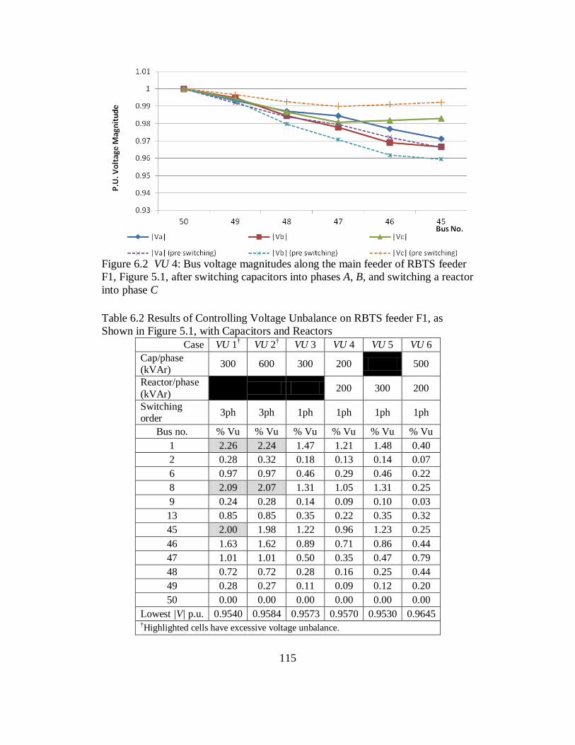
115
Figure 6.2 VU 4: Bus voltage magnitudes along the main feeder of RBTS feeder
F1, Figure 5.1, after switching capacitors into phases A, B, and switching a reactor
into phase C
Table 6.2 Results of Controlling Voltage Unbalance on RBTS feeder F1, as
Shown in Figure 5.1, with Capacitors and Reactors
Case VU 1† VU 2
† VU 3 VU 4 VU 5 VU 6
Cap/phase (kVAr)
300 600 300 200 500
Reactor/phase (kVAr)
200 300 200
Switching order
3ph 3ph 1ph 1ph 1ph 1ph
Bus no. % Vu % Vu % Vu % Vu % Vu % Vu
1 2.26 2.24 1.47 1.21 1.48 0.40
2 0.28 0.32 0.18 0.13 0.14 0.07
6 0.97 0.97 0.46 0.29 0.46 0.22
8 2.09 2.07 1.31 1.05 1.31 0.25
9 0.24 0.28 0.14 0.09 0.10 0.03
13 0.85 0.85 0.35 0.22 0.35 0.32
45 2.00 1.98 1.22 0.96 1.23 0.25
46 1.63 1.62 0.89 0.71 0.86 0.44
47 1.01 1.01 0.50 0.35 0.47 0.79
48 0.72 0.72 0.28 0.16 0.25 0.44
49 0.28 0.27 0.11 0.09 0.12 0.20
50 0.00 0.00 0.00 0.00 0.00 0.00
Lowest |V| p.u. 0.9540 0.9584 0.9573 0.9570 0.9530 0.9645 †Highlighted cells have excessive voltage unbalance.

116
Figure 6.3 VU 5: Bus voltage magnitudes along the main feeder of RBTS feeder
F1, Figure 5.1, after switching in a 300 kVAr reactor on phase C
Figure 6.4 VU 6: Bus voltage magnitudes along the main feeder of RBTS feeder
F1, Figure 5.1, after switching 500 kVAr/ph caps into phase A and B, and a 200
kVAr reactor into phase C
6.3 Distributed generation
As indicated in the literature on DG in distribution systems and in subsection
1.6 of this dissertation, voltage regulation issues and the possibility of bidirection-
al power flows exist [82]-[86]. Contemporary research in DG has seen efforts re-

117
lated to power injections in distribution systems. The literature focuses on renew-
able DG and local storage for voltage control, peak shaving and other control op-
tions [92]-[94], [96].
The illustrations developed here explore implications of DG in the estimation
of three-phase, possibly unbalanced distribution networks. In the three-phase un-
balanced circuit of the RBTS for feeder F1, shown in Figure 5.1, two wind gener-
ators are placed at buses 8 and 13. These buses are at the primary of a three-phase
distribution transformer at the high side rated 11 kV. Each DG unit is assumed to
inject approximately 1.0 MW peak output (nameplate value) following the profile
shown in Appendix G. In practice, this may be an aggregated capacity of DG.
Note that present standards for interconnecting DG [45] strictly state that no ac-
tive voltage regulation is allowed for non-utility controlled installations at less
than 10 MW. To this point, reactive power injections for this illustration are as-
sumed to be zero. The presence of DG in distribution systems is illustrated in ex-
amples DG1, DG2, and DG3 as shown in Table 6.3.
Table 6.3 Examples Illustrating the Presence of DG in Distribution Systems
Example Description
DG1
Example illustrates bidirectional power flows in the dis-
tribution system. Power flows in different directions in
each phase for some line segments. Power also flows into
the transmission system.
DG2
This example illustrates the possible voltage rise on the
distribution feeder. Based on estimator calculations, DG
reactive output is altered to mitigate voltage rise.
DG3 In this illustration, energy storage (batteries) and DG are
used to perform energy management and peak shaving.

118
Bidirectional flows with DG (Example DG1)
The illustration commences with 1.0 MW of wind DG being injected into the
circuit of RBTS feeder F1 in the early morning hours (HE3). Note that at this
time, DG injection is at a maximum value and load is near a minimum value (see
Appendix G). As anticipated, DG injection is larger than the load so power flows
into the substation node and into the distribution primary and subtransmission
network.
Perhaps more interesting is the direction of power flows on branches 48-47
and 47-46 where the direction of power flowing on phases is different for each
phase. Also note that at bus 47, phase C power flows into this bus from both bus-
es 48 and 46 (see Fig. 6.5). The three-phase network model is needed to observe
this result since positive sequence analysis may fail to explicitly display the power
flow direction in individual phases.
The main feeder bus voltage profile corresponding to the loading and power
flow condition as indicated in Figure 6.5 is shown in Figure 6.6. Note that there
is voltage rise on all three phases at the end of the feeder (DG located at the last
node on the system) and that phase-C voltage rises above the source voltage. If
the substation voltage was 1.05 p.u. (not uncommon), safe operating voltage
would be violated according to ANSI C84. ‘Range A’.
This bidirectional flow phenomenon impacts coordination of protective devic-
es [26], regulation of voltages using step-type line voltage regulators [25], [96]
and system operation with uncertain loading. Investigations where net-load seen

119
by the substation transformer is positive yielded expected power flow and voltage
profile results; therefore, additional results are not shown here. Similarly, charac-
teristic solar generation that ramps up during daytime hours along with load
yielded conventional power flow and voltage profile results and, therefore, are not
elaborated here. Note that in practice, it is also possible to have net injection at a
substation when solar injections exceed loads.
Figure 6.5 One-line diagram, loads and injections for RBTS feeder F1 with DG at
HE3 (Example DG1)

120
Figure 6.6 Bus voltage profile for the loading condition of RBTS feeder F1 shown
in Figure 6.5 (Example DG1)
Voltage control using an estimator signal to alter DG power factor (Example
DG2)
One possible application of the distribution state estimator for voltage control
includes the provision of a signal to adjust distributed generator power factor to
regulate local voltage. That is, estimator results may be interpreted near real-time;
this information may be used as inputs to inverters (e.g., rooftop PV), or power
factor control elements (e.g., capacitors) to absorb or inject reactive power as a
means to counteract undesirable voltage levels. For example, the case of main
feeder bus voltages shown in Figure 6.6 may favor a reactive power absorption by
the DG to reduce voltage on phase C; although, given the bus voltage magnitudes
shown they are within acceptable tolerances for both magnitude and unbalance.
For this illustration, the DG power factor is varied by changing the set-point
of the unit to absorb VArs. The target value of bus 45 phase C voltage magnitude

121
is 1.0 p.u. To obtain this, reactive power is absorbed by the generator at 30 kVAr
/ phase and 40 kVAr / phase. The results have been plotted in Figure 6.7. Bus
voltage on phase C is reduced to 1.0 p.u. when 40 kVAr / phase is absorbed by the
distributed generator. This equates to a DG power factor of 0.993 leading.
Figure 6.7 Bus voltage profile for the loading condition of RBTS feeder F1 shown
in Figure 6.5 when DG power factor is changed to absorb reactive power, exam-
ple DG2
Using energy storage and DG to reduce peak demand, example DG3
One possible alternative to controlling both bidirectional flows and voltage
rises due to DG injections is the inclusion of energy storage elements such as fly-
wheels, batteries or others. Energy storage elements may function as ipso facto
loads on the distribution system. They typify controllable load elements since
charging and discharging may be performed at desired time intervals.
Energy storage elements may be used to smooth variability due to intermittent
generation, perform price arbitrage, supplement reliability efforts to keep loads
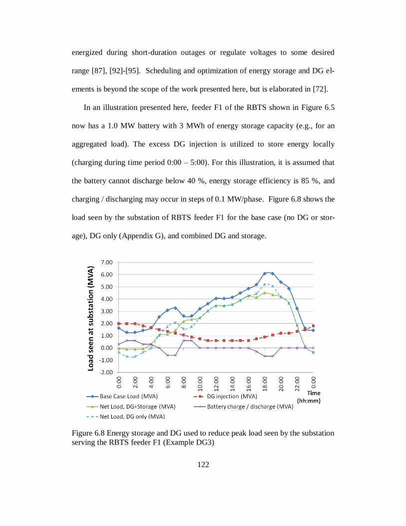
122
energized during short-duration outages or regulate voltages to some desired
range [87], [92]-[95]. Scheduling and optimization of energy storage and DG el-
ements is beyond the scope of the work presented here, but is elaborated in [72].
In an illustration presented here, feeder F1 of the RBTS shown in Figure 6.5
now has a 1.0 MW battery with 3 MWh of energy storage capacity (e.g., for an
aggregated load). The excess DG injection is utilized to store energy locally
(charging during time period 0:00 – 5:00). For this illustration, it is assumed that
the battery cannot discharge below 40 %, energy storage efficiency is 85 %, and
charging / discharging may occur in steps of 0.1 MW/phase. Figure 6.8 shows the
load seen by the substation of RBTS feeder F1 for the base case (no DG or stor-
age), DG only (Appendix G), and combined DG and storage.
Figure 6.8 Energy storage and DG used to reduce peak load seen by the substation
serving the RBTS feeder F1 (Example DG3)

123
Net peak load is reduced from 6.2 MW to 4.5 MW. The battery is charged in
the early morning (low load), and after the morning peak. The battery discharges
during morning peak and system peak. Note that voltage unbalance in these cases
may be handled as indicated in section 6.2.
6.4 Large Scale Simulation System test bed (LSSS) illustration
The large scale simulation system (LSSS) test bed is described in subsection
4.4. Bus voltage magnitudes and angles for the solved power flow case for the
transmission and networked subtransmission superstructure is shown in Figure
6.9. Illustrations consist of estimating all bus voltages magnitudes and angles for
the entire LSSS test bed in three-phase detail.
Tables 6.3 – 6.6 present specified active and reactive power of loads installed
at each load bus for the peak (HE18) load condition. Loads are presented in kW
and kVAr. Missing phases are omitted from the tables. Note that data for feeder
F1 are presented in previous chapters (also see Appendix F). Also note that data
for the IEEE 34 bus test system are presented in [131]. Each feeder has unique
characteristics and loading patterns for the purpose of analysis. Feeder F2 serves
larger industrial loads at 11 kV, all three-phase, balanced. Feeder F3 has lightly
loaded B phase. Feeder F4 has lightly loaded A phase. Feeder F6 has heavily
loaded A phase and lightly loaded C phase.

124
Figure 6.9 Transmission network and bus 3 distribution subtransmission network
for the LSSS test bed where transmission buses are numbered from 101-107, and
bus 103 is bus 3 at 138 kV as indicated in [38]
Table 6.4 Specified load on Each Phase for RBTS Feeder F2, Figure 4.3 Feeder F2 Specified load at each phase, P (kW), Q (kVAr) Bus No. Pa Qa Pb Qb Pc Qc
8 345.68 175 335.51 165 335.51 160 9 335.51 160 335.51 160 345.68 165 10 335.51 165 345.68 165 335.51 170
Total 1016.70 500 1016.7 490 1016.7 495
Table 6.5 Specified load on Each Phase for RBTS Feeder F3, Figure 4.3 Feeder F3 Specified load at each phase, P (kW), Q (kVAr) Bus No. Pa Qa Pb Qb Pc Qc
11 510 220 340 150
12 510 200 255 115 85 40 13 255 115 170 80 425 225 14 277.50 125 370 175 277.50 105 15
775 350
16 182.77 100 161.88 70 177.55 90 17 174.07 93 174.07 85 174.07 90
Total 1909.34 853.00 1470.95 675.00 1914.12 900.00

125
Table 6.6 Specified load on Each Phase for RBTS Feeder F4, Figure 4.3 Feeder F4 Specified load at each phase, P (kW), Q (kVAr) Bus No. Pa Qa Pb Qb Pc Qc
18 170 60 425 200 255 115 19 313.32 155 156.66 70 52.22 22 20
836.70 400
21
836.70 400
22 83.67 40 251.01 115 502.02 205 23 292.85 110 259.38 110 284.48 110 24 284.48 110 276.11 100 276.11 120
Total 1144.31 475.00 2204.86 995.00 2206.53 972.00
Table 6.7 Specified load on Each Phase for RBTS Feeder F6, Figure 4.3 Feeder F6 Specified load at each phase, P (kW), Q (kVAr) Bus No. Pa Qa Pb Qb Pc Qc
32 340 155 255 111 255 115 33 510 220 255 115 85 39 34 425 180 170 70 255 100 35 340 125 255 115 255 105 36 170 85 425 201 255 115 37 208.88 100 313.32 150
38 208.88 100 313.32 150
Total 2202.76 965.00 1986.64 912.00 1105.00 474.00
6.5 An application of distribution state estimation for demand response,
energy and power management, example DR1
An application of the distribution state estimator is illustrated for demand re-
sponse on the LSSS network. In DR applications, enabled loads are asked to cur-
tail load during periods of high demand. Billinton in [38] identifies that 20 % of
the RBTS loads are available for curtailment. In practice, it may be difficult to
determine exact curtailment and response to commands. The utility must ensure
that curtailing load does not exacerbate voltage unbalance or increase flows in
heavily loaded branches.

126
Example DR1
The subsequent illustration presents the application of the estimator in a net-
work with DR. Each load is assumed able to curtail up to 20 %. However, actual
load curtailment may vary significantly. In the illustration, loads may curtail be-
tween 5.0 - 20.0 %. The exact value of load curtailment at non-measured buses is
not known, but will be estimated. Demands at each load bus for the pre-DR case
(base case) are presented in Table 6.4 - Table 6.7. The reduced load at each feed-
er is shown in Table 6.8 - Table 6.11. The estimator is used to calculate injections
/ loads and voltage profiles. Power flow at the substation is assumed to be meas-
ured; however, where substation flows are not measured, these flows may be cal-
culated.
Table 6.8 Load Curtailed for RBTS Feeder F2, Figure 4.3, Example DR 1
Feeder F2 Percentage load remaining after curtailment at each phase (%), and substation load (MW) example DR1
Metered bus
Bus No. Pa Pb Pc Qa Qb Qc 8 80.87 91.58 80.63 80.87 91.58 80.63 Y 9 89.87 88.26 83.50 89.87 88.26 83.50 Y 10 88.97 92.42 85.01 88.97 92.42 85.01 Y
Substation 0.882 0.925 0.845 0.437 0.449 0.415
Table 6.9 Load Curtailed for RBTS Feeder F3, Figure 4.3, Example DR 1
Feeder F3 Percentage load remaining after curtailment at each phase (%), and substation load (MW) example DR1
Metered bus
Bus No. Pa Pb Pc Qa Qb Qc 11 80.87 91.58
80.87 91.58
Y 12 89.87 88.26 83.50 89.87 88.26 83.50 N 13 88.97 92.42 85.01 88.97 92.42 85.01 N 14 90.39 80.47 93.04 90.39 80.47 93.04 N 15
89.66
89.66 Y 16 90.71 94.26 94.78 90.71 83.67 94.78 Y 17 89.09 83.67 90.68 89.09 83.67 90.68 Y
Substation 1.689 1.296 1.764 0.843 0.621 0.910
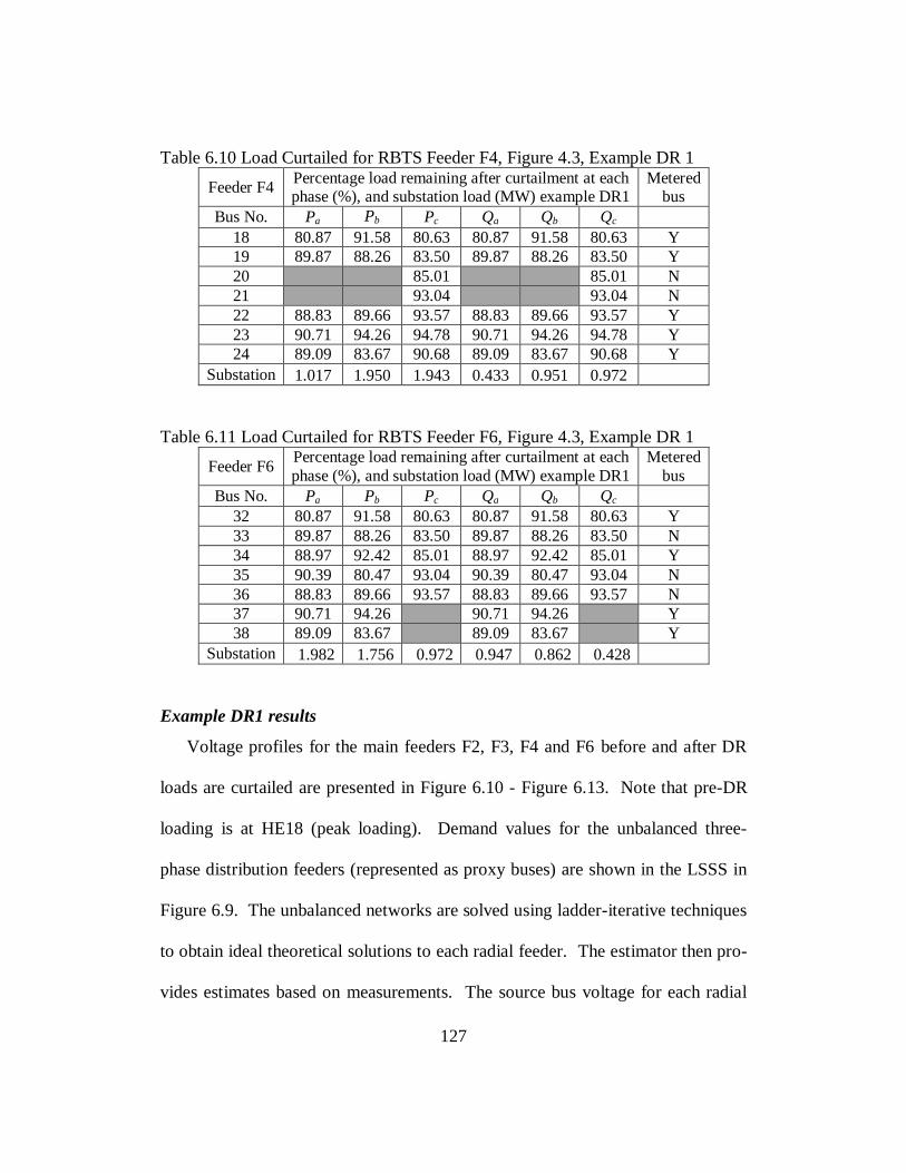
127
Table 6.10 Load Curtailed for RBTS Feeder F4, Figure 4.3, Example DR 1
Feeder F4 Percentage load remaining after curtailment at each phase (%), and substation load (MW) example DR1
Metered bus
Bus No. Pa Pb Pc Qa Qb Qc 18 80.87 91.58 80.63 80.87 91.58 80.63 Y 19 89.87 88.26 83.50 89.87 88.26 83.50 Y 20
85.01
85.01 N 21
93.04
93.04 N 22 88.83 89.66 93.57 88.83 89.66 93.57 Y 23 90.71 94.26 94.78 90.71 94.26 94.78 Y 24 89.09 83.67 90.68 89.09 83.67 90.68 Y
Substation 1.017 1.950 1.943 0.433 0.951 0.972
Table 6.11 Load Curtailed for RBTS Feeder F6, Figure 4.3, Example DR 1
Feeder F6 Percentage load remaining after curtailment at each phase (%), and substation load (MW) example DR1
Metered bus
Bus No. Pa Pb Pc Qa Qb Qc 32 80.87 91.58 80.63 80.87 91.58 80.63 Y 33 89.87 88.26 83.50 89.87 88.26 83.50 N 34 88.97 92.42 85.01 88.97 92.42 85.01 Y 35 90.39 80.47 93.04 90.39 80.47 93.04 N 36 88.83 89.66 93.57 88.83 89.66 93.57 N 37 90.71 94.26
90.71 94.26
Y 38 89.09 83.67
89.09 83.67
Y
Substation 1.982 1.756 0.972 0.947 0.862 0.428
Example DR1 results
Voltage profiles for the main feeders F2, F3, F4 and F6 before and after DR
loads are curtailed are presented in Figure 6.10 - Figure 6.13. Note that pre-DR
loading is at HE18 (peak loading). Demand values for the unbalanced three-
phase distribution feeders (represented as proxy buses) are shown in the LSSS in
Figure 6.9. The unbalanced networks are solved using ladder-iterative techniques
to obtain ideal theoretical solutions to each radial feeder. The estimator then pro-
vides estimates based on measurements. The source bus voltage for each radial

128
feeder is identified from Figure 6.9. Note that profiles for feeder F1 are presented
in previous sections. Post curtailment ideal and estimated loads are presented in
Table 6.12 - Table 6.15. The transmission network of the RBTS is re-solved after
load curtailment. The reduced load at bus 3 causes a substation bus voltage rise.
Figure 6.10 Bus voltage magnitudes before and after DR at HE18 on main feeder
buses for RBTS feeder F2, example DR1
Figure 6.11 Bus voltage magnitudes before and after DR at HE18 on main feeder
buses for RBTS feeder F3, example DR1

129
Figure 6.12 Bus voltage magnitudes before and after DR at HE18 on main feeder
buses for RBTS feeder F4
Figure 6.13 Bus voltage magnitudes before and after DR at HE18 on main feeder
buses for RBTS feeder F6
Table 6.12 Ideal and Estimated Post-Curtailment Loads, Feeder F2, Example DR1
Bus Pa Pb Pc Qa Qb Qc
Post-curtailment loads, ideal (MW, MVAr)
8 0.280 0.307 0.271 0.142 0.151 0.129
9 0.302 0.296 0.289 0.144 0.141 0.138
10 0.299 0.319 0.285 0.147 0.152 0.145
Post-curtailment loads, estimated (MW, MVAr)
8 0.281 0.309 0.271 0.146 0.155 0.132
9 0.303 0.298 0.289 0.147 0.144 0.141
10 0.300 0.321 0.285 0.149 0.155 0.147

130
Table 6.13 Ideal and Estimated Post-Curtailment Loads, Feeder F3, Example DR1
Bus Pa Pb Pc Qa Qb Qc
Post-curtailment loads, ideal (MW, MVAr)
11 0.412 0.311
0.178 0.137
12 0.458 0.225 0.071 0.180 0.101 0.033
13 0.227 0.157 0.361 0.102 0.074 0.191
14 0.251 0.298 0.258 0.113 0.141 0.098
15
0.725
0.327
16 0.166 0.153 0.168 0.091 0.066 0.085
17 0.155 0.146 0.158 0.083 0.071 0.082
Post-curtailment loads, estimated (MW, MVAr)
11 0.419 0.312
0.208 0.147 12 0.466 0.226 0.072 0.214 0.108 0.036
13 0.229 0.158 0.366 0.115 0.077 0.210
14 0.252 0.301 0.262 0.124 0.148 0.108
15
0.736
0.379
16 0.166 0.154 0.170 0.096 0.068 0.090
17 0.155 0.146 0.158 0.085 0.072 0.084
Table 6.14 Ideal and Estimated Post-Curtailment Loads, Feeder F4, Example DR1
Bus Pa Pb Pc Qa Qb Qc
Post-curtailment loads, ideal (MW, MVAr)
18 0.137 0.389 0.206 0.049 0.183 0.093
19 0.282 0.138 0.044 0.139 0.062 0.018
20
0.711
0.340
21
0.673
0.322
22 0.074 0.225 0.470 0.036 0.103 0.192
23 0.266 0.244 0.270 0.100 0.104 0.104
24 0.253 0.231 0.250 0.098 0.084 0.109
Post-curtailment loads, estimated (MW, MVAr)
18 0.138 0.403 0.204 0.049 0.205 0.104
19 0.283 0.143 0.043 0.144 0.068 0.020
20
0.708
0.400
21
0.694
0.366 22 0.075 0.232 0.468 0.036 0.112 0.219
23 0.266 0.249 0.269 0.103 0.110 0.113
24 0.254 0.234 0.250 0.101 0.088 0.114

131
Table 6.15 Ideal and Estimated Post-Curtailment Loads, Feeder F6, Example DR1
Bus Pa Pb Pc Qa Qb Qc
Post-curtailment loads, ideal (MW, MVAr)
32 0.275 0.234 0.206 0.125 0.102 0.093
33 0.458 0.225 0.071 0.198 0.101 0.033
34 0.378 0.157 0.217 0.160 0.065 0.085
35 0.307 0.205 0.237 0.113 0.093 0.098
36 0.151 0.381 0.239 0.076 0.180 0.108
37 0.189 0.295
0.092 0.145
38 0.186 0.262
0.089 0.126
Post-curtailment loads, estimated (MW, MVAr)
32 0.281 0.232 0.207 0.142 0.109 0.095
33 0.469 0.224 0.071 0.229 0.109 0.033
34 0.386 0.157 0.218 0.182 0.069 0.088
35 0.312 0.205 0.238 0.125 0.098 0.101
36 0.153 0.381 0.239 0.081 0.194 0.111
37 0.192 0.295
0.095 0.149
38 0.188 0.262
0.093 0.132
Figure 6.14 Solving the RBTS transmission network after DR load curtailment

132
6.6 Discussion of results
Discussion of voltage unbalance studies, examples VU1-VU6
An example was presented that studies the problem of voltage unbalance, and
potential mitigation measures that may be required in a utility system. The com-
bination of capacitor / reactor switching was used to control voltage magnitudes
and reduce unbalance. The capacitor switching into the circuit reduces the need
for reactive power from the source and concomitantly boosts bus voltage magni-
tude. However, results showed that conventional switching of three-phases of the
cap bank would not help the under voltage issue, but would not combat unbal-
ance. Single phase control of the capacitor bank in example VU3 provides the best
overall impact on both reducing voltage unbalance and increasing magnitudes.
Examples shown are intended to illustrate new applications of static VAr sys-
tems in distribution systems. That is, mitigation measures to voltage unbalance
issues using single-phase switching of shunt reactive elements may be required in
smart distribution systems, examples of this are shown.
Discussion of DG and storage results, examples DG1-DG3
Smart distribution systems may benefit from higher penetration of DG, DER,
storage technology or PHEV technologies. These technologies may provide an-
cillary voltage balancing as part of normal operations. Example DG1 illustrates
the potential impacts of bidirectional flows in a distribution feeder. Power flow
may be in different directions in each phase, and may flow towards the transmis-
sion system. This is a significant departure from conventional distribution system

133
operations. Implications for protection, coordination and energy management ex-
ist but are not elaborated here. The distribution system state estimator may be
used as a tool to alert operators to these issues as they occur, and to capture oper-
ating state before / during events.
Example DG2 illustrates the use of DG in conjunction with estimator created
signals to regulate feeder bus voltages. Illustration DG3 explores implications of
energy storage, load balancing and peak shaving in the Smart Grid environment.
The estimator may be utilized as a tool to assist operators in scheduling storage,
energy management, and simultaneously maintaining adequate voltage profiles.
Discussion of LSSS illustration example DR1
The illustration of demand response load curtailment shows a potential appli-
cation of the distribution state estimator. Loads are randomly reduced between
5.0 – 20.0 %. Note that not all loads are measured. The state estimator is then
used to calculate bus voltage magnitudes on the feeder, and obtain estimates of
individual loads, both measured and not measured. The estimator provides good
estimates of loads after curtailment. The calculations and estimates are all done in
three-phase detail.
Note the weakness in the analysis method used here: load curtailment in the
distribution system produces changes in the transmission (LSSS) network voltage
profile. However, in the foregoing analysis, the bus voltage magnitude at the sub-
station is held constant. As shown in Figure 6.14, the bus voltage at the substation
may change when loads are curtailed.

134
7. Conclusions, recommendations and future work
7.1 Contributions and concluding remarks
Distribution level focus areas of the Smart Grid initiative include: distribution
automation (DA), DMS system integration; increased operator control, and ex-
pansion of customer owned DG. System integrity, reliability, fault tolerance and
safety to consumers must be maintained. Future distribution systems may incor-
porate responsive loads, networking and more measurement devices – each of
these items are illustrated in this dissertation. To maximize the use of existing as-
sets and mitigate the need to expand large-generation portfolios, utilities and ISOs
may continue to extend their reach into distribution circuits. Monitoring and es-
timation of system changes become an important function in this environment.
DMS and distribution class state estimators may become a valuable tool in future
distribution infrastructure.
The unique characteristics of the distribution system necessitate different tools
for analysis when compared to transmission systems. Unique characteristics of
distribution networks are discussed in Chapter 1. The Smart Grid initiative items
discussed in the previous paragraph increase the complexity of distribution system
modeling and analysis. Thus, enhanced tools for modeling, simulation and analy-
sis are required. The distribution system state estimator is seen as one such tool to
be used in near the real-time analysis applications.
This dissertation presents the formulation of a linear state estimation algo-
rithm for distribution feeders. The estimator uses a weighted least squares formu-

135
lation and is developed in full three-phase detail. Reliance on measured data (i.e.
widely deployed smart meters) allows a non-iterative solution procedure. Main
and secondary contributions of this work are summarized in Table 7.1.
Table 7.1 Contributions of this research Category Contribution
Reliability and restoration
enhancement
Algorithms are developed and illustrated.
These algorithms present practical methods to study reliability in
future distribution systems.
Networking and rapid restoration are known to improve reliability;
methods such as the system status table and related algorithms pre-sent a framework around which these may be implemented
Distribution
system state
estimation
The formulation of a linear, three-phase distribution system state
estimator is presented. Practical considerations such as high r/x ra-
tios, laterals and unbalanced loads are included.
Noting the measurement infrastructure likely in future distribution
systems, the estimator utilizes available data to calculate system
state – even where no measurement data is available.
Pseudo-measurement data, historical loads and conventional meas-
urements and synchrophasors are utilized in the estimation formu-
lation; these are all likely in practical systems of the future.
The estimator performance is illustrated, along with applications to
voltage control, DG, and storage.
Implications of
the Smart Grid
initiative on
the future distribution
infrastructure
While details of the future infrastructure remain uncertain, trends
toward increased measurement availability are clear. The work in
this dissertation supports an advanced metering infrastructure.
DG installations include a range of technologies not detailed here.
The application and utilization of these technologies are enhanced
by distribution state estimation.
Protection and coordination is identified as a major area of concern
when operating principles change. Protection is likely to become more complex, but real-time monitoring of conditions may facili-
tate more complex networks.
7.2 General recommendations
Examples and illustrations presented in this dissertation are summarized here,
and general recommendations are made subsequently. Chapter 4 illustrates vari-
ous algorithms for distribution system reliability and restoration enhancement

136
through automation and switching. Chapter 5 illustrates the distribution system
state estimation algorithm formulation and performance. Chapter 6 investigates
voltage unbalance, mitigation options using shunt reactive elements, implications
of DG in the distribution system, and a sample of a large scale test system. The
illustrations presented throughout this report highlight various aspects of the esti-
mator formulation, performance and applications. Illustrations include:
Three-phase estimator formulation and performance
Inclusion of the characteristics of distribution systems in modeling, analy-
sis and distribution system state estimation (e.g., high r/x ratio, unbalance,
single phase laterals)
Estimator performance in the presence of noisy measurement data
Biased estimation to improve accuracy for the examples presented
Bad data detection on the system being studied
Applications in voltage control and mitigation of voltage unbalance
Applications in distributed generation including bidirectional flows
DG and voltage regulation based on estimator inputs
Applications for distributed resources, storage, energy management, and
peak shaving
Demand response and load curtailment in the LSSS network.

137
Table 7.2 Discussion and Observations of Illustrations Presented
Illustration
topic Details / results Observations / conclusion
Reliability enhancement
Switching automation demon-strated on RYG, RBTS test beds
RYG: adding 4 interrupting de-vices may reduce E(U) by 50%
RBTS: 14% reduction in E(U)
RBTS: 7% reduction in SAIDI
Automation resulted in significant reliability im-
provements
Further improvements may be achieved via network-
ing, adding DG or storage
Unbiased three-
phase distribution system state estimation –
Example SE3
A state estimator algorithm for 3ϕ distribution was developed
The estimator is demonstrated on a radial 3ϕ RBTS feeder, F1,
on transmission bus 3
The algorithm runs in substation
computer DMS for monitoring, control and to alert operators
Bus voltage magnitudes are well estimated with highly uncertain
load data in examples shown
Distribution circuit loading is highly uncertain
Measurement redundancy may significantly increase estimator accuracy
Bus voltage magnitudes and line currents are well
estimated
Biased three-phase distribution system state estimation
Examples SE2, SE3a are recre-ated with biased measurements
Resulting estimates are approx-imately 85% more accurate than unbiased estimates for examples
shown here
Variance of calculated, linear-ized currents may be approxi-
mated
Weighting measurements may provide better angle
and line current estimates
Weights may be assigned in various ways
Heuristically, selecting the
largest % uncertainty as a variance is appropriate
Voltage unbalance
Voltage unbalance is observed
for heavy load cases
Methods to mitigate voltage
unbalance include single phase switching of shunt capacitor /
reactor (VAr) devices
The preferred result is obtained by switching in 2 phases of a
capacitor bank (VU3)
Unbalanced loads / lat-
erals, and mutual coupling of untransposed lines caus-
es voltage unbalance
Estimator based control options are calculated
Single phase control of shunt devices may provide
a finer detail of control
Distributed generation (DG)
and storage
Voltage rise and bidirectional
flows are illustrated with DGs
Estimator created signals are used to adjust DG VAr output to
regulate bus voltages
Storage/energy management are used to reduce peak load
Near real-time monitoring allows greater control of
available DG and storage resources as illustrated

138
7.3 Future work
The three-phase distribution estimator formulation presented here will ac-
commodate networked feeders. Networked distribution primary feeders may be-
come more prevalent in future distribution systems. In other applications, net-
worked distribution secondaries may also be used. Effects of networking on loss
reduction and voltage regulation may be explored further as future work. A po-
tential application of the estimator may be selective networking to alter voltage
profiles, control power flows or reduce losses. The protection and coordination of
protective devices are an important consideration for the future distribution infra-
structure, especially where selective networking and DG is concerned.
Perhaps the most significant future work involves the modeling and simula-
tion of systems that incorporate both transmission and distribution networks. For
example, analysis methods capable of solving transmission networks as positive
sequence networks with distribution sub-systems as three-phase detailed networks
may be of interest in the future power system infrastructure. This concept may
have applications in networks with DG, storage or controllable elements, and
where power-marketing concepts such as the LMP may be extended into the dis-
tribution system model.
As a final remark, an important element of future work surely includes actual
implementation in a functioning distribution system.

139
REFERENCES
[1] 0th Congress of United States, “Smart Grid,” Title XIII, Energy Inde-
pendence and Security Act of 2007, Washington DC, December 2007.
[2] Office of Electric Transmission and Distribution, United States Depart-
ment of Energy, “Grid 2030: A National Vision for Electricity’s Second
00 Years,” Washington DC, April 2003.
[3] Office of Electricity Delivery and Energy Reliability, United States De-
partment of Energy, “The Smart Grid – An Introduction,” Washington
DC, 2008 [Available online]: http://www.oe.energy.gov/
DocumentsandMedia/DOE_SG_Book_Single_Pages.pdf.
[4] Office of Electricity Delivery and Energy Reliability, United States De-
partment of Energy, “What the Smart Grid Means to You (Utilities) and
the People You Serve,” Washington DC, 2009, [Available online]:
http://www.oe.energy.gov/DocumentsandMedia/Utilities.pdf.
[5] Office of Electricity Delivery and Energy Reliability, United States De-
partment of Energy, “What the Smart Grid Means To You (Technology
Providers) And The People You Serve,” Washington DC, 2009, [Availa-
ble online]: http://www.oe.energy.gov/DocumentsandMedia/Technology
Providers.pdf.
[6] United States Department of Energy, “Smart Grid System Report,” Wash-
ington DC, July 2009 [Available online]: http://www.oe.energy.gov/
DocumentsandMedia/SGSRMain_090707_lowres.pdf
[7] B. R. Sathyanarayanan, G. T. Heydt, M. Crow, F. Meng, “Test Bed Evalu-
ation of Future Power Distribution Systems with Renewable Resources,”
North American Power Symposium (NAPS), Starkville, MS 2009, pp. 1-8.
[8] A. Q. Huang, M. L. Crow, G. T. Heydt, J. P. Zheng, S. J. Dale, “The Fu-
ture Renewable Electric Energy Delivery and Management (FREEDM)
system: the Energy Internet,” Proceedings of the IEEE, v. 99, no. , Janu-
ary 2011, pp. 1-16.

140
[9] F. I. Denny, D. E. Dismukes, Power System Operations and Electricity
Markets, CRC Press, New York, NY, 2002.
[10] M. Ilic, F. Galiana, L. Fink, Power Systems Restructuring – Engineering
and Economics, Kluwer Academic Publishers, Massachusetts, 1998.
[11] Y. Song, X. Wang, Operation of Market-oriented Power Systems, Spring-
er, New York, 2003.
[12] M. Kezunovic, G. T. Heydt, C. DeMarco, T. Mount, “Is Teamwor the
Smart Solution?,” IEEE Power and Energy Magazine, v. 7, No. 2, March,
2009 pp. 69 -78.
[13] Z. Alaywan, “Impact of Deregulation on System Operation in California,”
CIGRE/IEEE Power Engineering Society International Symposium, 2005,
pp. 24-30.
[14] R. L. Chen, S. Sabir, “The Benefits of Implementing Distribution Automa-
tion and System Monitoring in the Open Electricity Mar et,” Proceeding
of the IEEE Canadian Conference on Electrical and Computer Engineer-
ing, v. 2, Toronto, 2001, pp. 825-830.
[15] V. Vittal, “Consequence and Impact of Electric Utility Industry Restruc-
turing on Transient Stability and Small-Signal Stability Analysis,” Pro-
ceedings IEEE, v. 88, no. 2, February 2000, pp. 196 – 207.
[16] American Wind Energy Association, “Renewable Portfolio Standards,”
[Available Online:]
http://www.awea.org/policy/renewables_portfolio_standard.html.
[17] U.S. Department of Energy, Database of State Incentives for Renewables
and Efficiency, [Available online]: www.dsireusa.org]
[18] U.S. Environmental Protection Agency, Renewable Portfolio Standards,
[Available online]: http://www.epa.gov/chp/state-policy/renewable.html

141
[19] U.S. Energy Information Administration, Annual Energy Review 2009,
August 19, 2010 [Available online]: http://www.eia.gov/electricity
[20] U.S. Energy Information Administration, Annual Energy Outlook 2011,
April 26, 2011 [Available online]: http://www.eia.gov/electricity
[21] California State Senate Bills 1078, and 107, California Renewables Port-
folio Standard [Available online]: http://www.cpuc.ca.gov/PUC/energy/
Renewables
[22] “Solar statistics for the state of California,” [Available online]:
http://www.californiasolarstatistics.ca.gov/reports/agency_stats/
[23] A. Walsh, T. Fallon, “ESB Networ s Smart Grid Demonstration Pilot,”
IEEE General Meeting, Detroit, MI, July 2011
[24] J. A. Momoh, Electric Power Distribution, Automation, Protection and
Control, CRC Press, New York, NY, 2008.
[25] W. H. Kersting, Distribution System Modeling and Analysis, CRC Press,
New York, NY, 2007.
[26] J. Burke, Power Distribution Engineering – Fundamentals and Applica-
tions, New York, NY: Marcel Dekker, 1994.
[27] H. L. Willis, Power Distribution Planning Reference Book, Marcel Dek-
ker, New York, NY, 1997.
[28] J. D. Glover, M. S. Sarma, T. Overbye, Power System Analysis and De-
sign, 4th ed., Thomson Learning, 2008.
[29] R. Allan, R. Billinton, Reliability Evaluation of Power Systems, 2nd ed.,
Springer, 1996.
[30] R. Billinton, R. Ringlee, A. Wood, Power System Reliability Calculations,
MIT Press, Cambridge, MA, 1973.

142
[31] R. Brown, Electric Power Distribution Reliability, New York, NY: Marcel
Dekker, 2002.
[32] R. P. Fanning, “Implementation of Networ ed Primary and Secondary
Distribution Systems for U.S. Utilities,” Proceedings IEEE Power Engi-
neering Society General Meeting, July 2003, vol. 4, pp. 2425 – 2429.
[33] R. E. Brown, "Network Reconfiguration for Improving Reliability in Dis-
tribution Systems," in Proceedings 2003 IEEE PES General Meeting, To-
ronto, Canada, July 2003.
[34] W. Steeley, C. Perry, M. Vaziri, “Interconnection of Distributed Energy
Resources in Secondary Distribution Networ Systems,” EPRI white pa-
per 1012922, Technical Update, Palo Alto, CA, December 2005.
[35] G. Heydt, “Improving Distribution Reliability (the N9 problem) by the
Addition of Primary Feeders,” IEEE Transactions on Power Delivery, v.
19, No. 1, Jan. 2004, pp. 434-435.
[36] G. T. Heydt, Electric Power Quality, 2nd ed., Stars in a Circle Publica-
tions, Scottsdale, AZ, 1991.
[37] R. Billinton, S. Kumar, N. Chowdhury, K. Chu, K. Debnath, L. Goel, E.
Khan, P. Kos, G. Nourbakhsh, J. Oteng-Odjei, “A Reliability Test System
for Educational Purposes – Basic Data,” IEEE Transactions on Power Sys-
tems, v. 4, No. 3, August 1989, pp. 1238 -1244.
[38] R. Billinton, S. Jonnavithalu, “A Test System for Teaching Overall Power
System Reliability Assessment,” IEEE Transactions on Power Delivery, v.
11, No. 4, November 1996, pp. 1670 – 1676.
[39] R. Billinton, Reliability Assessment of Electrical Power Systems Using
Monte Carlo Methods, Plenum Publishers, New York, 1994.
[40] R. Billinton, W. Wangdee, “Delivery Point Reliability Indices of a Bul
Electric System Using Sequential Monte Carlo Simulation,” IEEE Trans-
actions on Power Delivery, vol. 21, no. 1, January, 2006, pp. 345-352.

143
[41] V. Werner, D. Hall, R. Robinson, C. Warren, “Collecting and Categoriz-
ing Information Related to Electric Power Distribution Interruption
Events: Data Consistency and Categorization for Benchmar ing Surveys,”
IEEE Transactions on Power Delivery, v. 21, No. 1, January 2006, pp. 480
– 483.
[42] A. J. Wood, B. F. Wollenberg, Power Generation Operation and Control,
2nd
ed., John Wiley & Sons, 2007.
[43] B. Stott, “Fast Decoupled Load Flow,” IEEE Transactions PAS, v. PAS
91, September-October, 1972, pp. 1955–1959.
[44] G. Heydt, Computer Analysis Methods for Power Systems, 2nd ed., Stars
in a Circle Publications, Scottsdale, AZ, 1996.
[45] IEEE Standard 1547, Standard for Interconnecting Distributed Resources
with Electric Power Systems, Piscataway, NJ, 2009.
[46] I. Roytelman, S. M. Shahidehpour, “State Estimation for Electric Power
Distribution Systems in Quasi Real-Time Conditions,” IEEE Transactions
on Power Delivery, vol. 8, no. 4, October, 1993, pp. 2009-2015.
[47] M. E. Baran, A. W. Kelley, “State Estimation for Real-Time Monitoring
of Distribution Systems,” IEEE Transactions on Power Systems, v. 9, no.
3, August 1994, pp. 1601–1609.
[48] M. E. Baran, A. W. Kelley, “A Branch-Current Based State Estimation
Method for Distribution Systems,” IEEE Transactions on Power Systems,
v. 10, no. 1, February 1995, pp. 483–491.
[49] C. N. Lu, J. H. Teng, W. E. Liu, “Distribution System State Estimation,”
IEEE Transactions on Power Systems, v. 10, no. 1, February 1995, pp.
229–240.
[50] A. P. S. Meliopoulos, F. Zhang, “Multiphase Power Flow and State Esti-
mation for Power Distribution Systems,” IEEE Transactions on Power
Systems, v. 11, no. 2, May 1996, pp. 939–946.

144
[51] J. Wan, K. Miu, “Weighted Least Squares Method for Load Estimation in
Distribution Networ s,” IEEE Transactions on Power Systems, v. 18, no.
4, November 2003, pp. 1338–1345.
[52] R. Singh, B. C. Pal, R. A. Jabr, “Choice of Estimator for Distribution Sys-
tem State Estimation,” IET Generation, Transmission and Distribution, v.
3, no. 7, 2009, pp. 666–678.
[53] E. Manitsas, R. Singh, B. Pal, G. Strbac, “Modeling of Pseudo-
Measurements for Distribution System State Estimation,” Proceedings IET
CIRED Smart Grids for Distribution, Frankfurt, 2008, pp. 1–4.
[54] R. Hoffman, “Practical State Estimation for Electric Distribution Net-
wor s,” IEEE PES Power Systems Conference and Expositions, October,
2006, pp. 510-517.
[55] M. Powal o, K. Rudion, P. Komarnic i, J. Blumschein, “Observability of
the Distribution System,” CIRED International Conference on Electricity
Distribution, June 2009, pp. 8-11.
[56] M. E. Baran, J. Jung, T. McDermott, “Topology Error Identification Using
Branch Current State Estimation for Distribution Systems,” Transmission
and Distribution Conference and Exposition, Asia and Pacific, October,
2009, pp. 1-4.
[57] A. Abur, H. Singh, H. Liu, W. N. Klingensmith, “Three Phase Power
Flow for Distribution Systems with Dispersed Generation,” 4th PSCC,
Sevilla, June 2002, Session 11, Paper 3, pp. 1-7.
[58] T. Gonen, Electric Power Distrbution System Engineering, 2nd
ed., CRC
Press, Boca Raton, FL, 2007.
[59] M. W. Davis, R Broadwater, J. Hambric , “Modeling and Testing of Un-
balanced Loading and Voltage Regulation,” NREL report number
NREL/SR-581-41805, July, 2007.
[60] P. Pillay, P. Hofmann, M. Manyage, “Derating of Induction Motors Oper-
ating With a Combination of Unbalanced Voltages and Over or

145
Undervoltages,” IEEE Transactions of Energy Conversion, v. 7, no. 4,
December 2002, pp. 485-491.
[61] P. Pillay, M. Manyage, “Definitions of Voltage Unbalance,” IEEE Power
Engineering Review, May 2001, pp. 50-51.
[62] Pacific Gas and Electric, “Voltage Unbalance and Motors,” October,
2009.
[63] Motors and Generators, National Electrical Manufacturers Association
(NEMA) Publication No. MG 1-1998.
[64] J. Eto, K. LaCommare, “Trac ing the Reliability of the U.S. Electric Pow-
er System: An Assessment of Publicly Available Information Reported to
State Public Utility Commissions,” LBNL Report LBNL-1092E, October
2008. [Available online]: http://certs.lbl.gov/pdf/lbnl1092e-puc-reliability
-data.pdf
[65] Consortium for Electric Reliability Technology Solutions, “Microgrid
Concept,” [Available online]: http://certs.lbl.gov/certs-der-micro.html
[66] S. Chowdhury, S. P. Chowdhury, P. Crossley, Microgrids and Active Dis-
tribution Networks, Institution of Engineering and Technology: Renewa-
ble Energy Series, 2009.
[67] M. Shahidehpour, “Role of Smart Microgrid in a Perfect Power system,”
IEEE PES General Meeting, Minneapolis, MN, July, 2010, pp. 1.
[68] J. Northcote-Green, R. G. Wilson, Control and Automation of Electrical
Power Distribution Systems, CRC Press, Boca Raton, FL, 2006.
[69] Singh, N.; Kliokys, E.; Feldmann, H.; Kussel, R.; Chrustowski, R.;
Joborowicz, C., “Power system modelling and analysis in a mixed energy
management and distribution management system,” IEEE Transactions on
Power Systems, v. 13, no.3, Aug. 1998, pp. 1143-1149.

146
[70] Open Systems International (OSI), “Distribution Management Systems,”
[Available online]: http://www.osii.com/solutions/products/distribution-
management.asp
[71] Operation Technology, Inc. (OTI) – Electrical Transient Analyzer Pro-
gram (ETAP), “Real-Time Distribution Management System,” [Available
online]: etap.com.
[72] B. S. Sathyanarayana, “A Roadmap for Distribution Energy Management
via Multiobjective Optimization,” Proceedings IEEE General Meeting, Ju-
ly, 2010.
[73] S. Ma , “Smart Meters Serving As Synchro-Sensors For Smart Distribu-
tion Grid Applications,” IEEE PES General Meeting, Detroit, MI, 20 .
[74] D. Wight, et al., “Assessment of Demand Response and Advanced Meter-
ing – Staff Report,” U.S. Federal Energy Regulatory Commission, Febru-
ary 2011.
[75] K. Lindsey, “Practical Aspects of Using Line Sensors in the Field,” Pro-
ceedings IEEE General Meeting, Minneapolis, MN, July 2010.
[76] K. Lindsey, “Practical Aspects of Using Line Sensors In the Field,” Pro-
ceedings IEEE PES General Meeting, Detroit, MI, July, 2011.
[77] D. Carty, M. Atanacio, “PMUs and Their Potential Impact on Real-time
Control Center Operations,” Proceedings IEEE General Meeting, Minne-
apolis, MN, July 2010.
[78] G. T. Heydt, S. Bhatt, “Present and Future Trends and Needs in Electric
Power Quality Sensors and Instrumentation,” Journal of Electric Machines
and Power Systems, v. 27, No. 7, July, 1999, pp. 691-700.
[79] T. J. Browne, J. W. Stahlhut, G. T. Heydt, W. T. Jewell, R. Bezawada,
“Innovative and Massively Deployed Sensors in Electric Power Systems,”
IEEE PES General Meeting, July 2008, pp. 1-6.
147
[80] “Solar PV Interconnection Guidelines, Maps and Requirements,” [Availa-
ble online]: http://www.sce.com/EnergyProcurement/renewables/spvp-
ipp/spvp-ipp.htm
[81] U.S. Department of Energy, et al. “20% Wind Energy by 2030 - Increas-
ing Wind Energy’s Contribution to U.S. Electricity Supply,” report
DOE/GO-102008-2567, July, 2008 [Available online]:
www.nrel.gov/docs/fy08osti/41869.pdf
[82] A. Mills, R. Wiser, “Implications of Wide-Area Geographic Diversity for
Short-Term Variability of Solar Power,” Lawrence Ber eley National La-
boratory Report 3884E Sept. 2010, [Available online]:
http://eetd.lbl.gov/ea/EMS/reports/lbnl-3884e.pdf
[83] S. Ven ataraman, U. Helman, et al., “Integration of Renewable Resources
– Operational Requirements and Generation Fleet Capability at 20 %
RPS,” California Independent System Operator, August, 20 0.
[84] B.K. Parsons, Y. Wan, B. Kirby, “Wind Farm Power Fluctuations, Ancil-
lary Services, and System Operating Impact Analysis Activities in the
United States,” July 200
[85] J. W. Smith, R. Dugan, W. Sunderman, “Distribution Modeling and Anal-
ysis of High Penetration PV,” IEEE General Meeting, Detroit, MI, July
2011
[86] M. P. Wa efield, “Smart Distribution System Research in EPRI’s Smart
Grid Demonstration Initiative,” IEEE General Meeting, Detroit, MI, July
2011
[87] J. Mic ey, “Using Load Resources to Meet Ancillary Service Require-
ments in the ERCOT Market: A Case Study,” Proceedings IEEE General
Meeting, Minneapolis, MN, July 2010.
[88] X. Zhang, R. Fields, K. Abreu, “Financial Benefits of Implementing De-
mand Response in CAISO Mar et,” Proceedings IEEE General Meeting,
Minneapolis, MN, July 2010.
148
[89] L. B. Lave, K. Spees, “Demand Response and Electricity Mar et Efficien-
cy,” The Electricity Journal, vol. 20, no. 3, April, 2007, pp. 69-85.
[90] E. J. Paulson, “Demand response as ancillary services in the PJM RTO,”
Proc. IEEE PES General Meeting, June, 2005, San Francisco, CA, pp.
1575-1578.
[91] R. Mu erji, “Demand Response in the NYISO Mar ets,” Proc. IEEE
Power Systems Conference and Exposition, March, 2011, Phoenix, AZ,
pp. 1-2.
[92] S. Windergren, H. Kir ham, “Smart Grid – Transforming Power System
Operations,” Proceedings IEEE General Meeting, Minneapolis, MN, July
2010.
[93] H. Johal, D. Manz, K. O’Brien, J. Kern, “Grid Integration of Energy Stor-
age,” Proc. IEEE PES General Meeting, Detroit, MI, July 20 , pp. -2.
[94] G. D. Rodriguez, “A Utility Perspective of the Role of Energy Storage in
the Smart Grid,” Proc. IEEE PES General Meeting, Minneapolis, MN, Ju-
ly 2010, pp. 1-2.
[95] D. Manz, N. Miller, H. Elahi, “Energy storage for the grid,” A presenta-
tion to the New York Independent System Operator, 2011 [Available
online]:
www.nyiso.com/public/webdocs/committees/environmental_advisory_cou
ncil/meeting_materials/2011-05-13/Energy_Storage_-
GE_Energy_Consulting.pdf
[96] R. Dugan, M. McGranaghan, S. Santoso, H. Beaty, Electrical Power Sys-
tems Quality, 2nd
ed., McGraw Hill, New York, 2002.
[97] Itron, Smart Meter Specifications Data Sheets, 2011 [Available online]:
www.itron.com.
[98] E. Kyria ides, G. T. Heydt, “Synchronized Measurements in Power Sys-
tem Operation: International Practices and Research Issues,” IEEE PES
General Meeting, July 2009, pp. 1-3.

149
[99] IEEE Standard C37.118-2005, Standard for Synchrophasors for Power
Systems, Piscataway, NJ, 2005.
[100] J. S. Thorpe, A. G. Phad e, K. J. Karimi, “Real-Time Voltage-Phasor
Measurements for Static State Estimation,” IEEE Trans. on Power Appa-
ratus and Systems, v. PAS-104, no. 11, November 1985, pp. 3098 – 3 106.
[101] J. S. Thorpe, A. G. Phad e, S. H. Horowitz, M. M. Begovic, “Some Ap-
plications of Phasor Measurements to Adaptive Protection,” IEEE Trans.
on Power Systems, v. 3, no. 2, May 1988, pp. 791 – 798.
[102] A. G. Phad e, “Recent Advances in Monitoring, Protection, and Control
of Power Systems,” Proceedings, Joint International Power Conference,
Athens Power Tech (APT), Athens, September, 1993, pp. 326 – 331.
[103] Damir Novosel, et al., Performance Requirements Task Team (PRTT),
“Performance Requirements Part II - Targeted Applications: State Estima-
tion,” Eastern Interconnection Phasor Project (EIPP), North American
Synchrophasor Initiative, July, 2006, pp. 1-33 [Available online]:
http://www.naspi.org/resources/archive/archiveresources.stm.
[104] A. Abur, “Impact of Phasor Measurements on State Estimation,” Interna-
tional Conference on Electrical and Electronics Engineering, November,
2009, pp. I3-I7.
[105] A. Abur, A. G. Exposito, Power System State Estimation – Theory and
Implementation, New York, NY: Marcel Dekker, 2004.
[106] F. C. Schweppe, E. J. Handschin, “Static State Estimation in Electric
Power Systems,” Proceedings IEEE, vol. 62, no. 7, July 974, pp. 972-
982.
[107] A. Monticelli, State Estimation in Electric Power Systems: A Generalized
Approach, Kluwer Academic Publishers, 1999.
[108] IEEE 1366, Guide for Electric Power Distribution Reliability Indices, Pis-
cataway, NJ, 2003.

150
[109] M. M. Adibi, Power System Restoration: Methodologies & Implementa-
tion Strategies, IEEE Press, 2000.
[110] C. C. Lui, S. J. Lee, S. S. Ven ata, “An Expert System Operational Aid
for Restoration and Loss Reduction of Distribution Systems,” IEEE
Transactions on Power Systems, v. 3, no. 2, 1988, pp. 619 – 626.
[111] K. Matsumoto, T. Sa aguchi, R. J. Kaf a, M. M. Adibi, “Knowledge
Based Systems as Operational Aids in Power System Restoration,” Pro-
ceedings of the IEEE, v. 80, no. 5, 1992, pp. 689-697.
[112] R. L. Wilde, “Effects of Cold Load Pic up at the Distribution Substation
Transformer,” IEEE Transactions on Power Apparatus and Systems, v.
PAS-104, no. 3, 1985, pp. 704-710.
[113] E. Mondon, B. Heilbronn, Y. Harmand, O. Paillet, H. Fargier, “MARS:
An Aid for Networ Restoration After a Local Disturbance,” Proceedings
Power Industry Computer Application Conference, May 1991, pp. 344-
349.
[114] Y. M. Par , K. H. Lee, “Application of an Expert System to Power System
Restoration in Sub-Control Center,” IEEE Trans. on Power Systems, v.
12, no. 2, May 1997, pp. 629-635.
[115] Q. Zhour, D. Shirmohammadi, W. H. E. Liu, “Distribution Feeder Recon-
figuration for Service Restoration and Load Balancing,” IEEE Transac-
tions on Power Systems, v. 12, no. 2, May 1997, pp. 724-729.
[116] Tropos networ s, “Outage Management: The Electric Utility’s No.
Headache,” A technology brief by TROPOS networ s, July 2007, [Avail-
able Online]: http://www.tropos.com/pdf/technology_briefs/tropos_
techbrief_outage_mgmt.pdf.
[117] D. A. Haughton, G. T. Heydt, “Smart Distribution System Design: Auto-
matic Reconfiguration for Improved Reliability,” Proceedings IEEE Gen-
eral Meeting, Minneapolis, MN, July, 2010.

151
[118] H. Brown, D. A. Haughton, G. T. Heydt, S. Suryanarayanan, “Some Ele-
ments of Design and Operation of a Smart Distribution System,” Proceed-
ings IEEE Power and Energy Society Transmission and Distribution Con-
ference and Exposition, New Orleans, LA, April, 2010.
[119] G. Heydt, “The Next Generation of Power Distribution Systems,” IEEE
Transactions on Smart Grid, accepted for publication, 2010.
[120] M. Fiedler, Special Matrices and their Applications in Numerical Mathe-
matics, Martinus Nijhoff Publishers (a member of Kluwer Academic Pub-
lishers Group), 1986.
[121] J.A. Bondy, U.S.R. Murty, Graph Theory-Graduate Texts in Mathematics,
Springer, 2008.
[122] B. Liu, H. Lai, Matrices in Combinatorics and Graph Theory, Boston,
MA: Kluwer Academic Publishers, 2000.
[123] IEEE Standard 1366-2003, Guide for Electric Power Distribution Relia-
bility Indices, Piscataway, NJ, 2003.
[124] R.V. Patel, A. J. Laub, P. M Van Dooren, Numerical Linear Algebra
Techniques for Systems and Control, IEEE Press, 1994.
[125] A.S. Householder, The Theory of Matrices in Numerical Analysis, Dover,
NY, 1964.
[126] M. B Allen III, E. L Isaacson, Numerical Analysis for Applied Science,
John Wiley and Sons, NY, 1998.
[127] A. S. Deif, Advanced Matrix Theory for Scientists and Engineers, Abacus
Press, U.K. 1982.
[128] G. H. Golub, C. F. Van Loan, Matrix Computations, 3rd
ed., John Hopkins
University Press, MD, 1996.

152
[129] R. Ebrahimian, R. Baldic , “State Estimator Condition Number Analysis,”
IEEE Transactions on Power Systems, v. 16, no. 2, May, 2001, pp. 273-
279.
[130] D. A. Haughton, G. T. Heydt, “A Linear State Estimation Formulation for
Smart Distribution Systems,” accepted for publication in IEEE Transac-
tions on Power Systems, 2012.
[131] W. H. Kersting, et al., “Radial Distirubiton Test Feeders,” IEEE Transac-
tions on Power Systems, v. 6, no. 3, 1991, pp. 975-985.
[132] D. Montgomery, G. C. Runger, N. F. Hubele, Engineering Statistics, 3rd
.
ed., Wiley, 2004.
[133] Bharadwaj Ranganathan Sathyanarayana, “Sensitivity-based Pricing and
Multiobjective Control for Energy Management in Power Distribution
Systems,” PhD Thesis, Arizona State University, Tempe AZ, July, 2012
[134] D. A. Haughton, G. T. Heydt, “Synchronous Measurements in Power Dis-
tribution Systems,” chapter in “Control and Optimization Methods for
Electric Smart Grids, A. Cha rabortty and M. Ilić editors, Springer, Pub-
lishers, New York, 2012, Part III, pp. 295 – 312.

153
APPENDIX A
POWER FLOW RESULTS OF DIFFERENT MODELING ASSUMPTIONS

154
Appendix A. Power flow results of different modeling assumptions
This appendix demonstrates the effect of using an approximate line impedance
model versus the exact line impedance model. Note that results show slight dif-
ferences, but these differences may be significant enough to impact control ac-
tions and alarms based on algorithms that detect voltage magnitude difference.
Table A.1 Base Case Comparison of Voltage Magnitudes from an Exact and Ap-
proximate Model
Case C1 – Base case
Bus No.
Exact model (p.u.) Approximate model (p.u.) Difference
† (%)
|Va| |Vb| |Vc| |Va| |Vb| |Vc|
1 0.9880 0.9893 1.0021 0.9905 0.9906 0.9979 -0.25 -0.14 0.42
2 0.9872 0.9901
0.9896 0.9914
-0.24 -0.13 0.00
3
1.0016
0.9980 0.00 0.00 0.36
4
0.9889
0.9901
0.00 -0.12 0.00
5
1.0000
0.9972 0.00 0.00 0.28
6 0.9944 0.9938 0.9997 0.9959 0.9946 0.9974 -0.15 -0.08 0.23
7 0.9971
0.9976
-0.05 0.00 0.00
8 0.9880 0.9893 1.0022 0.9905 0.9907 0.9979 -0.25 -0.14 0.43
9 0.9873 0.9902
0.9896 0.9914
-0.24 -0.13 0.00
10
1.0016
0.9980 0.00 0.00 0.36
11
0.9890
0.9902
0.00 -0.12 0.00
12
1.0000
0.9972 0.00 0.00 0.28
13 0.9944 0.9938 0.9998 0.9959 0.9947 0.9974 -0.15 -0.08 0.23
14 0.9971
0.9977
-0.05 0.00 0.00
45 0.9885 0.9898 1.0023 0.9909 0.9910 0.9983 -0.24 -0.13 0.40
46 0.9903 0.9898 1.0021 0.9925 0.9910 0.9985 -0.22 -0.12 0.36
47 0.9935 0.9916 1.0005 0.9953 0.9926 0.9978 -0.18 -0.10 0.27
48 0.9951 0.9945 1.0000 0.9964 0.9952 0.9979 -0.13 -0.07 0.20
49 0.9977 0.9984 0.9996 0.9982 0.9987 0.9987 -0.05 -0.03 0.09
50 1.0000 1.0000 1.0000 1.0000 1.0000 1.0000 0.00 0.00 0.00 †
Difference calculated as (Vexact – Vapprox) / Vexact

155
Perhaps the most revealing visualization of the impact of different modeling
methods is to observe the bus voltage magnitudes along the main three-phase
feeder of the RBTS feeder F1, as shown in Figure 5.1. The following figures
show voltage magnitude differences between modeling the exact detail based on
line geometry, versus an approximate model for the main 11 kV feeder buses of
the RBTS feeder F1.
Table A.2 Case C5 Comparison of Voltage Magnitudes from an Exact and Ap-
proximate Model
Case C5 – Heavy load 3
Bus
No.
Exact model (p.u.) Approximate model (p.u.) Difference
† (%)
|Va| |Vb| |Vc| |Va| |Vb| |Vc|
1 0.9511 0.9610 1.0075 0.9543 0.9615 1.0010 -0.34 -0.06 0.65
2 0.9507 0.9610
0.9539 0.9615
-0.34 -0.06 0.00
3
0.9953
0.9897 0.00 0.00 0.56
4
0.9601
0.9607
0.00 -0.07 0.00
5
0.9903
0.9860 0.00 0.00 0.44
6 0.9704 0.9720 0.9916 0.9728 0.9726 0.9880 -0.24 -0.05 0.37
7 0.9821
0.9829
-0.08 0.00 0.00
8 0.9582 0.9679 1.0075 0.9613 0.9685 1.0010 -0.33 -0.05 0.65
9 0.9581 0.9679
0.9613 0.9685
-0.33 -0.06 0.00
10
1.0007
0.9951 0.00 0.00 0.56
11
0.9663
0.9670
0.00 -0.07 0.00
12
0.9971
0.9928 0.00 0.00 0.43
13 0.9790 0.9807 0.9984 0.9813 0.9812 0.9948 -0.24 -0.05 0.36
14 0.9889
0.9897
-0.08 0.00 0.00
45 0.9613 0.9685 1.0062 0.9645 0.9691 1.0000 -0.33 -0.06 0.62
46 0.9677 0.9697 1.0034 0.9708 0.9704 0.9978 -0.32 -0.07 0.56
47 0.9762 0.9764 0.9994 0.9788 0.9770 0.9951 -0.27 -0.06 0.43
48 0.9818 0.9834 0.9990 0.9838 0.9838 0.9959 -0.20 -0.04 0.32
49 0.9913 0.9944 0.9993 0.9921 0.9945 0.9979 -0.08 -0.02 0.13
50 1.0000 1.0000 1.0000 1.0000 1.0000 1.0000 0.00 0.00 0.00 †
Difference calculated as (Vexact – Vapprox) / Vexact

156
Figure A.1 Bus voltage magnitudes at main feeder buses for detailed and approx-
imate model, Case C2: heavy load 1
Figure A.2 Bus voltage magnitudes at main feeder buses for detailed and approx-
imate model, Case C3: heavy load 2
Figure A.3 Bus voltage magnitudes at main feeder buses for detailed and approx-
imate model, Case C4: heavy load 2 with shunt capacitor at bus 48

157
Figure A.4 Bus voltage magnitudes at main feeder buses for detailed and approx-
imate model, Case C5: heavy load 3 (peak)
Figure A.5 Bus voltage magnitudes at main feeder buses for detailed and approx-
imate model, Case C6: light load

158
APPENDIX B
FORWARD / BACKWARD LADDER ITERATIVE
POWER FLOW ALGORITHM

159
Appendix B. Forward / backward ladder iterative power flow algorithm
Figure B.1 and Figure B.2 outline basic steps in the forward sweep of the al-
gorithm used to calculate the three-phase voltages on the radial distribution sys-
tem. Note that the substation bus is taken as the slack bus/root node and all for-
ward paths to end-nodes are traced for connectivity, voltage calculated at next up-
stream node until all nodes are processed.
Figure B.1 Forward sweep algorithm overview 1 of 2

160
Figure B.2 Forward sweep algorithm overview 2 of 2

161
Figure B.3 and Figure B.4 present the steps of the backward sweep algorithm that
is used to calculate bus voltages and line flows in the radial distribution system.
The algorithm starts at an arbitrary end-node, and calculates back to each junction
node until all nodes are analyzed. The program terminates when the source bus
voltage has been calculated.
Figure B.3 Backward sweep algorithm overview 1 of 2
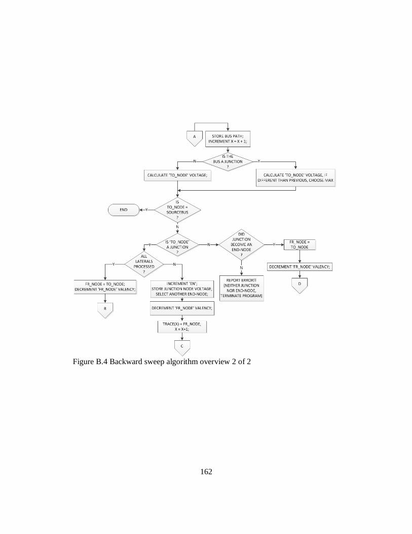
162
Figure B.4 Backward sweep algorithm overview 2 of 2

163
APPENDIX C
CONDITION NUMBER OF A MATRIX

164
Appendix C. Condition number of a matrix
References [124]-[128] provide detailed discussions concerning matrix theory
and condition number. It is especially important to consider the conditioning of a
matrix when a digital computer is used to solve the system of equations or com-
pute solution estimates. A matrix is said to be ill-conditioned if small errors in the
set of equations that describe the system, or small perturbations to the measure-
ment vector, cause large errors in the calculation of the state vector (or estimates).
Conversely, a well conditioned matrix is expected to produce less magnification
of error terms in the final solutions; however, state vector errors when small per-
turbations in the measurement vector may still be present.
As discussed in Chapter 3, common sources of ill-conditioning related to the
power system state estimation formulation include: a large proportion of injection
current measurements, long and short lines connected to the same bus and large
weighting factors applied to virtual measurements [105][129]. Using Equation
3.19, the condition number of the following matrices may be evaluated.
A = 0
0 B
.00 0.999
0.999
The singular values (and eigenvalues in this case) of A are obviously [1, 1].
Therefore, the condition number of A is found to be unity,
κ(A) = 1.
Conversely, by observation, B appears to be close to singularity, the single value
decomposition produces values of [1.995, 0.0015] (also eigenvalues of B), and
the condition number of B is,

165
κ(B) = 1333.
Quite obviously, A is a much better conditioned matrix as compared to B.
Figure C.1 summarizes a discussion from [124]. The following discussion re-
lates Figure C.1 to the state estimation problem. Given an exact data set, d, and a
transformation (set of equations) given by the function, f, the true solution to this
problem may be denoted as f(d). For a well-conditioned system described by the
function f, given an approximation (such as an estimate or sample) of the data set,
d*, the well conditioned system produces an f(d*) that is near f(d) (i.e. the true
solution). However, for an ill-conditioned function / system, f, the estimated/ cal-
culated solution, f(d*) may lie far away from the true solution, f(d). Generally the
more ill-conditioned the function f, the further the solution f(d*) may potentially
be away from the true solution f(d).
The same argument applies to an approximation of a function, f*, that approx-
imates the function, f. The approximation f* must also be well-conditioned for
the solution of f*(d) of the original data set, d, to lie near the true solution, f(d).
Implications in power system state estimation lie in the inherent ill-conditioned
nature of the set of equations used to solve power system problems. For example,
Newton Raphson is a first order Taylor series expansion that neglects higher order
derivatives. Also, in the system described in Chapter 3, the linearization of the
system of equations around an operating point creates the potential for inaccura-
cies in both the measurement function and measurement vector.

166
Figure C.1 Graphic representation of condition number, estimation and solution
accuracy
State estimation involves taking a sample of the data, d*, that is near d (i.e.
state measurements), and estimating the system parameters utilizing the system
model (i.e. f or f*). Note that in power system state estimation, the system model
is approximate (best model based on knowledge of the system and physical meas-
urements). It is apparent that a reasonably accurate solution depends on the sys-
tem model and how ‘close’ the measurements, d*, and how accurate the system
model, f* are to their true values.
The vector and matrix norms introduced in Chapter 3 provide a measure of
how close the true solution is to the estimated solution. A large norm of the re-
sidual vector indicates significant mismatch between measurement and estimate.
Conversely, a small value for norm indicates accurate match between estimated
and measured values. The state estimation formulation essentially tries to mini-
mize the norm of the residual of measurements to calculated solution. Generally
in the power operation center, a ‘close enough’ solution can give an operator

167
enough information to make decisions that continue to keep the grid in a stable
operating region.

168
APPENDIX D
ASSIGNING WEIGHTS TO CALCULATED CURRENTS

169
Appendix D. Assigning weights to calculated currents
An illustrative example of the approximate of current variance is presented
here. Note that given measurements Mk = {P, Q, Vm, δ}, and their variances
=
δ
, the variance of the calculated current may be approxi-
mated. The generic expectation for all measurements is = Mk. The expected
value of I, is a nonlinear function of Mk,
E( ) h(
P,
,
,
δ)
The variance may be approximated by
Va ( ) σ
h
σ
n
(D.1)
(D.2)
Given expectation of the real part of current,
E( ) Pcos δ sin δ
(D.3)
and imaginary part of current,
E( ) Psin δ cos δ
(D.4)

170
Variances are approximated by,
Va ( ) σ
σ
n
and
Va ( ) σ
2
σ
n
(D.5)
(D.6)
The Taylor series expansion is evaluated at each . The variance is then calcu-
lated according to Equation D.6. The expressions for real and imaginary parts of
the Taylor series expansion of the current equations are given in Table D.1.
Table D.1 Real and Imaginary Expressions for Taylor Series Expansion of
Real Quantities Imaginary Quantities
Pcos δ sin δ
E Psin δ cos δ
P
cos δ
P
sin δ
sin δ
cos δ
Pcos δ sin δ
Psin δ cos δ
δ
Psin δ Qcos δ
Iim
Pcos Qsin
σ
σ
=
σ =
σ
=
σ σ σ = σ
The illustrative example proceeds to calculate the expected current and ap-
proximate variance for the set of measurements provided in Table D.2. Resulting
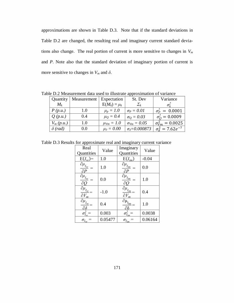
171
approximations are shown in Table D.3. Note that if the standard deviations in
Table D.2 are changed, the resulting real and imaginary current standard devia-
tions also change. The real portion of current is more sensitive to changes in Vm
and P. Note also that the standard deviation of imaginary portion of current is
more sensitive to changes in Vm and δ.
Table D.2 Measurement data used to illustrate approximation of variance
Quantity
Mk
Measurement Expectation
E(Mk) = k
St. Dev
Σk
Variance
σ
P (p.u.) 1.0 p = 1.0 σP = 0.01 σP
Q (p.u.) 0.4 Q = 0.4 σQ = 0.03 σ
Vm (p.u.) 1.0 Vm = 1.0 σVm = 0.05
δ (rad) 0.0 δ = 0.00 σδ=0.000873
Table D.3 Results for approximate real and imaginary current variance
Real
Quantities Value
Imaginary
Quantities Value
E 1.0 E -0.04
P 1.0
P 0.0
0.0
1.0
-1.0
0.4
δ 0.4
Iim
1.0
σ 0.003 σ
= 0.0038
σ 0.05477 σ = 0.06164

172
APPENDIX E
RYG TEST BED DATA

173
Appendix E. RYG test bed data
Table E.1 Bus Load Data for the RYG Test System
Bus No. P (MW) Q (MVAr) Circuit
1 Source - Red
2 0 -0.5 Red
3 2 1 Red
4 2 2 Red
5 1 0.4 Red
6 Source - Yellow
7 0.5 0 Yellow
8 0.5 0.5 Yellow
9 0 -0.5 Red
10 0.1 0.5 Red
11 0.5 0 Green
12 0.5 0.5 Yellow
13 0.5 0.5 Green
14 0.2 0 Red
15 0 -0.5 Green
16 0.2 0 Green
17 Source - Green
18 0 0 Green
19 1 0.5 Green
Total Demand 9 4.4 -
The following are for copper conductor at 60 Hz:
Red – 2/0; GMR, 0.01252 in.
Table E.2 Line Data for the RYG Test System
Line No. From Bus To Bus Length (km)
1 1 2 0.71
2 2 3 0.50
3 3 4 0.50
4 3 8 0.50
5 4 5 0.50
6 4 9 0.50
7 6 7 0.50
8 7 8 0.50
9 7 12 0.50
10 8 13 0.50
11 9 10 0.50
12 9 13 0.71
13 9 14 0.50
14 11 15 0.56
15 13 15 1.00
16 14 16 0.50
17 15 18 0.50
18 16 19 1.00
19 17 18 2.00
20 18 19 1.50
Yellow – No. 2 AWG; GMR, 0.00883 in.
Green – No. 2 AWG; GMR, 0.0093 in.

174
APPENDIX F
RBTS TEST BED MODELING AND LOAD ASSUMPTIONS

175
Appendix F. RBTS test bed modeling and load assumptions
This appendix contains data pertaining to the RBTS test bed. RBTS stands for
the Roy Billinton Test System after its creator. This data used in the state estima-
tion algorithm for feeder F1. The RBTS originally published in [38] presents a
realistic power system test bed. It contains generation, transmission and distribu-
tion networks. Line, load and bus data is given. Reliability analyses are shown.
The RBTS contains six buses in an HV transmission network. Five buses are
load buses. There are 11 large generators, 9 transmission lines, a total of 240 MW
of installed capacity, and 185 MW peak load. The system has 230 kV, 138 kV,
33 kV, 11 kV and 400 V voltages. The full RBTS system is small enough to be
studied and but large enough to be considered non-trivial. The largest distribution
sub-network in the RBTS is load bus 3 as depicted in Figure 4.2. Bus 3 has a
peak load of 85 MW, average load of 52.63 MW, and has various load types.
Figure F.1 presents the load profile as seen at the distribution transformer of
feeder F1. Load data used to create the load profile are provided in Table F.1
based on the average and peak provided in [38]; however, reasonable assumptions
are made to obtain a 24 hour load profile curve representative of a mixed load-
type feeder. Note that the data is provided by each phase, but loads are distribut-
ed along the feeder length according to Figure 4.2.
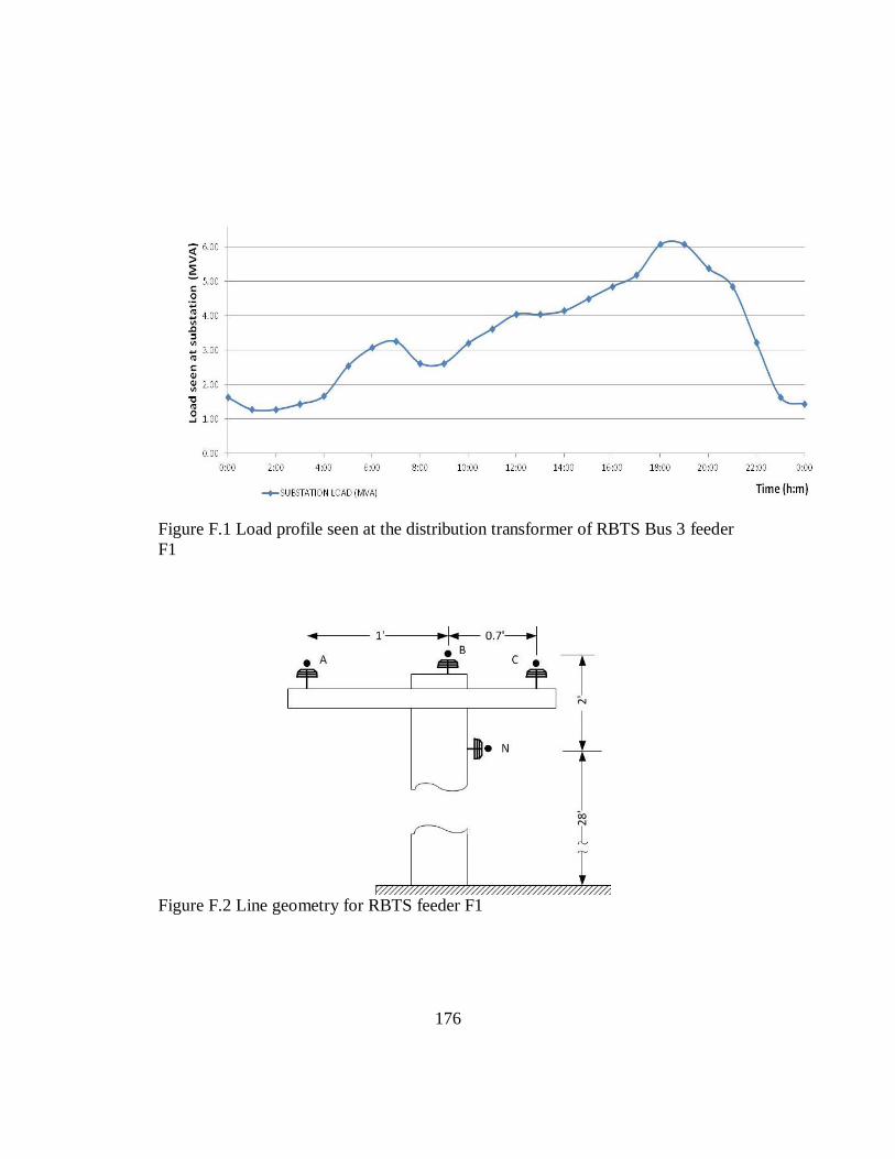
176
Figure F.1 Load profile seen at the distribution transformer of RBTS Bus 3 feeder
F1
Figure F.2 Line geometry for RBTS feeder F1
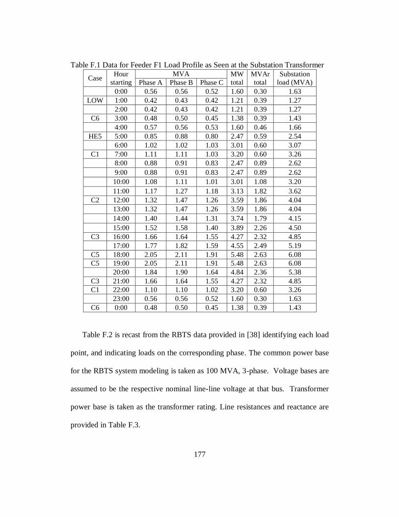
177
Table F.1 Data for Feeder F1 Load Profile as Seen at the Substation Transformer
Case Hour
starting MVA MW
total MVAr total
Substation load (MVA) Phase A Phase B Phase C
0:00 0.56 0.56 0.52 1.60 0.30 1.63
LOW 1:00 0.42 0.43 0.42 1.21 0.39 1.27
2:00 0.42 0.43 0.42 1.21 0.39 1.27
C6 3:00 0.48 0.50 0.45 1.38 0.39 1.43
4:00 0.57 0.56 0.53 1.60 0.46 1.66
HE5 5:00 0.85 0.88 0.80 2.47 0.59 2.54
6:00 1.02 1.02 1.03 3.01 0.60 3.07
C1 7:00 1.11 1.11 1.03 3.20 0.60 3.26
8:00 0.88 0.91 0.83 2.47 0.89 2.62
9:00 0.88 0.91 0.83 2.47 0.89 2.62
10:00 1.08 1.11 1.01 3.01 1.08 3.20
11:00 1.17 1.27 1.18 3.13 1.82 3.62
C2 12:00 1.32 1.47 1.26 3.59 1.86 4.04
13:00 1.32 1.47 1.26 3.59 1.86 4.04
14:00 1.40 1.44 1.31 3.74 1.79 4.15
15:00 1.52 1.58 1.40 3.89 2.26 4.50
C3 16:00 1.66 1.64 1.55 4.27 2.32 4.85
17:00 1.77 1.82 1.59 4.55 2.49 5.19
C5 18:00 2.05 2.11 1.91 5.48 2.63 6.08 C5 19:00 2.05 2.11 1.91 5.48 2.63 6.08
20:00 1.84 1.90 1.64 4.84 2.36 5.38
C3 21:00 1.66 1.64 1.55 4.27 2.32 4.85 C1 22:00 1.10 1.10 1.02 3.20 0.60 3.26
23:00 0.56 0.56 0.52 1.60 0.30 1.63
C6 0:00 0.48 0.50 0.45 1.38 0.39 1.43
Table F.2 is recast from the RBTS data provided in [38] identifying each load
point, and indicating loads on the corresponding phase. The common power base
for the RBTS system modeling is taken as 100 MVA, 3-phase. Voltage bases are
assumed to be the respective nominal line-line voltage at that bus. Transformer
power base is taken as the transformer rating. Line resistances and reactance are
provided in Table F.3.
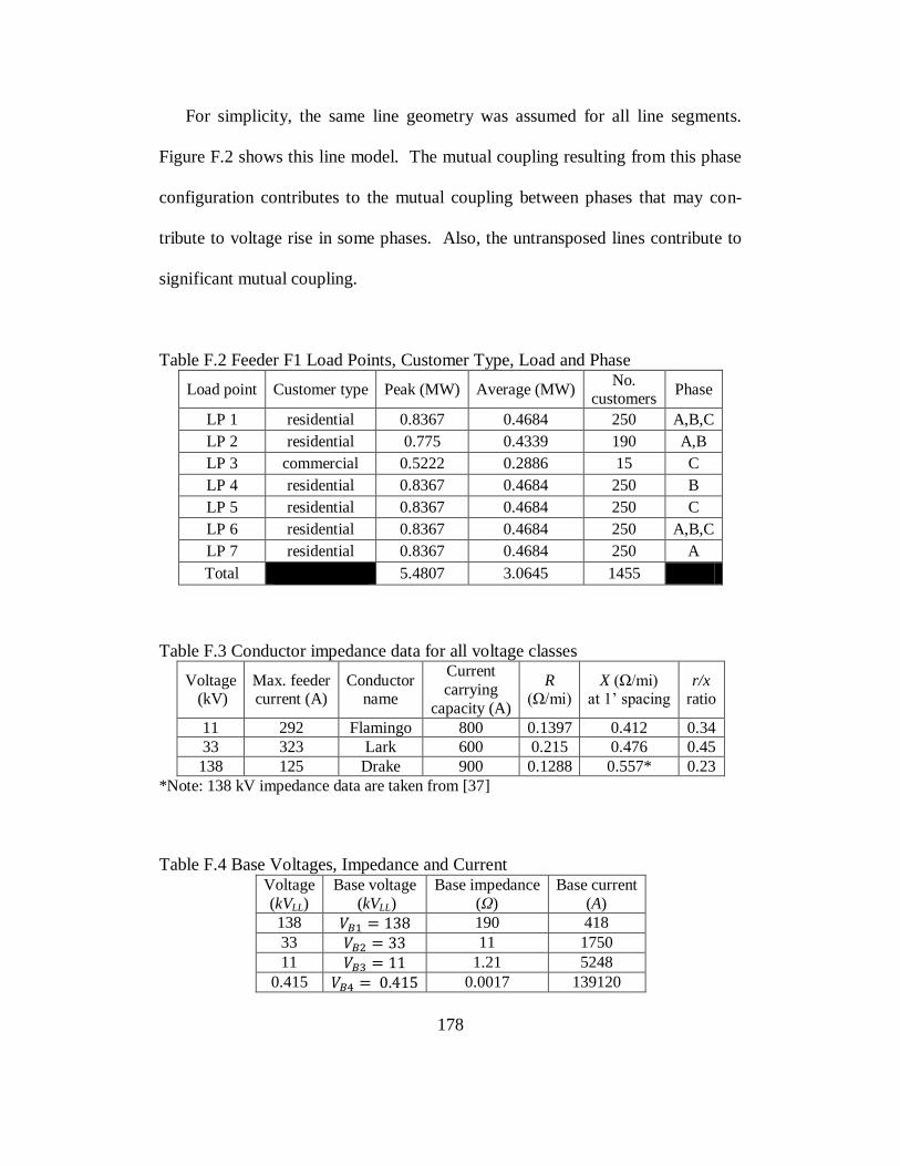
178
For simplicity, the same line geometry was assumed for all line segments.
Figure F.2 shows this line model. The mutual coupling resulting from this phase
configuration contributes to the mutual coupling between phases that may con-
tribute to voltage rise in some phases. Also, the untransposed lines contribute to
significant mutual coupling.
Table F.2 Feeder F1 Load Points, Customer Type, Load and Phase
Load point Customer type Peak (MW) Average (MW) No.
customers Phase
LP 1 residential 0.8367 0.4684 250 A,B,C
LP 2 residential 0.775 0.4339 190 A,B
LP 3 commercial 0.5222 0.2886 15 C
LP 4 residential 0.8367 0.4684 250 B
LP 5 residential 0.8367 0.4684 250 C
LP 6 residential 0.8367 0.4684 250 A,B,C
LP 7 residential 0.8367 0.4684 250 A
Total
5.4807 3.0645 1455
Table F.3 Conductor impedance data for all voltage classes
Voltage (kV)
Max. feeder current (A)
Conductor name
Current carrying
capacity (A)
R (Ω/mi)
X (Ω/mi) at ’ spacing
r/x ratio
11 292 Flamingo 800 0.1397 0.412 0.34 33 323 Lark 600 0.215 0.476 0.45 138 125 Drake 900 0.1288 0.557* 0.23
*Note: 138 kV impedance data are taken from [37]
Table F.4 Base Voltages, Impedance and Current Voltage (kVLL)
Base voltage (kVLL)
Base impedance (Ω)
Base current (A)
138 190 418 33 11 1750 11 1.21 5248
0.415 0.0017 139120

179
APPENDIX G
RBTS FEEDER F1 WITH DISTRIBUTED GENERATION

180
Appendix G. RBTS feeder F1 with distributed generation
Distributed generation is assumed on feeder F1 for a variety of studies. Stud-
ies include obtaining bus voltage profiles in the presence of distributed genera-
tion. DG locations were varied. Also, DG characteristic injection profile for wind
(night-peaking) and solar (day-peaking) was investigated. An approximate DG
penetration level of approximately 30 % was used in both cases; note that penetra-
tion level in this case is measured by the installed DG capacity relative to load.
The 24 hour load profile as seen by the substation transformer, DG injections,
and net load profile on RBTS feeder F1 are shown in Figure G.1 for solar DG in-
jections and Figure G.2 for typical wind injection profile. The nominal load val-
ues (with no DG) are assumed to be identical to those in 0. Values for solar and
wind injections for each hour of the 24 hour period are shown in Table G.1 (solar)
and Table G.2 (wind). Note that installed solar capacity is 1.5 MW, while in-
stalled wind capacity is approximately 2.0 MW. This represents 24.8 and 32.6
installed capacities of solar and wind respectively.
Figure G.1 Load, solar DG injection and net load profiles for a 24 hour peak day
as seen by RBTS feeder F1

181
Table G.1 Solar Injection Values (MW) and Net Load for 24 Hour Profile on
RBTS Feeder F1
Hour
starting MW
A MW
B MW
C MW Total
DG injection (MVA)
Net (MVA) [Load-Solar]
0:00 0.001 0.001 0.001 0.00 0.00 1.63 LOW 1:00 0.001 0.001 0.001 0.00 0.00 1.27 2:00 0.001 0.001 0.001 0.00 0.00 1.27 C6 3:00 0.001 0.001 0.001 0.00 0.00 1.43 4:00 0.001 0.001 0.001 0.00 0.00 1.66 5:00 0.001 0.001 0.001 0.00 0.00 2.53 6:00 0.001 0.001 0.001 0.00 0.00 3.07 C1 7:00 0.300 0.300 0.300 0.90 0.90 2.36 8:00 0.370 0.370 0.370 1.11 1.11 1.51 9:00 0.500 0.500 0.500 1.50 1.51 1.11 10:00 0.500 0.500 0.500 1.50 1.51 1.70 11:00 0.500 0.500 0.500 1.50 1.51 2.11 C2 12:00 0.500 0.500 0.500 1.50 1.51 2.54 13:00 0.500 0.500 0.500 1.50 1.51 2.54 14:00 0.500 0.500 0.500 1.50 1.51 2.64 15:00 0.500 0.500 0.500 1.50 1.51 2.99 C3 16:00 0.500 0.500 0.500 1.50 1.51 3.35 17:00 0.500 0.500 0.500 1.50 1.51 3.68 C5 18:00 0.400 0.400 0.400 1.20 1.20 4.88 C5 19:00 0.250 0.250 0.250 0.75 0.75 5.33 20:00 0.000 0.000 0.000 0.00 0.00 5.38 C3 21:00 0.000 0.000 0.000 0.00 0.00 4.85 C1 22:00 0.000 0.000 0.000 0.00 0.00 3.21 23:00 0.000 0.000 0.000 0.00 0.00 1.63 C6 0:00 0.000 0.000 0.000 0.00 0.00 1.43
Figure G.2 Load, wind DG injection and net load profiles for a 24 hour peak day
as seen by RBTS feeder F1
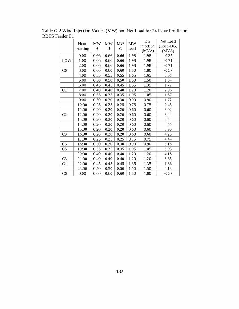
182
Table G.2 Wind Injection Values (MW) and Net Load for 24 Hour Profile on
RBTS Feeder F1
Hour
starting
MW
A
MW
B
MW
C
MW
total
DG
injection
(MVA)
Net Load
(Load-DG)
(MVA)
0:00 0.66 0.66 0.66 1.98 1.98 -0.35
LOW 1:00 0.66 0.66 0.66 1.98 1.98 -0.71
2:00 0.66 0.66 0.66 1.98 1.98 -0.71
C6 3:00 0.60 0.60 0.60 1.80 1.80 -0.37
4:00 0.55 0.55 0.55 1.65 1.65 0.01
5:00 0.50 0.50 0.50 1.50 1.50 1.04
6:00 0.45 0.45 0.45 1.35 1.35 1.72
C1 7:00 0.40 0.40 0.40 1.20 1.20 2.06
8:00 0.35 0.35 0.35 1.05 1.05 1.57
9:00 0.30 0.30 0.30 0.90 0.90 1.72
10:00 0.25 0.25 0.25 0.75 0.75 2.45
11:00 0.20 0.20 0.20 0.60 0.60 3.02
C2 12:00 0.20 0.20 0.20 0.60 0.60 3.44
13:00 0.20 0.20 0.20 0.60 0.60 3.44
14:00 0.20 0.20 0.20 0.60 0.60 3.55
15:00 0.20 0.20 0.20 0.60 0.60 3.90
C3 16:00 0.20 0.20 0.20 0.60 0.60 4.25
17:00 0.25 0.25 0.25 0.75 0.75 4.44
C5 18:00 0.30 0.30 0.30 0.90 0.90 5.18
C5 19:00 0.35 0.35 0.35 1.05 1.05 5.03
20:00 0.40 0.40 0.40 1.20 1.20 4.18
C3 21:00 0.40 0.40 0.40 1.20 1.20 3.65
C1 22:00 0.45 0.45 0.45 1.35 1.35 1.86
23:00 0.50 0.50 0.50 1.50 1.50 0.13
C6 0:00 0.60 0.60 0.60 1.80 1.80 -0.37

183
APPENDIX H
ILLUSTRATIVE EXAMPLES DESCRIBED

184
Appendix H. Illustrative Examples Described
Table H.1 summarizes illustrations presented throughout the dissertation.
Table H.1 Illustrative examples presented throughout this dissertation Example name Section Test bed Topic illustrated
RYG reliability /
restoration 4.6 RYG
Interrupting device location
RYG reliability 4.7 RYG Unserved energy vs. number of in-
terrupting devices
RBTS reliability
(7 cases) 4.8 RBTS
Automation
State estimation
(SE1, SE2, SE3) 5.1
RBTS,
Feeder F1
Unbiased estimation formulation.
No noise, and estimating under var-
ious loading conditions
Biased state estimation (SE1, SE2, SE3)
5.2
RBTS,
Feeder F1
Biased estimation formulation. No
noise, and estimating under various loading conditions
Bad data detection 5.3 RBTS,
Feeder F1 Detecting bad data when load on one phase is measured in error
Voltage unbalance and
control (VU1 - VU6) 6.2
RBTS,
Feeder F1
Voltage unbalance cases with vari-ous shunt reactive values
DG – bidirectional flows (DG1)
6.3 RBTS,
Feeder F1 DG and bidirectional flows
DG – voltage control
(DG2) 6.3
RBTS,
Feeder F1
Estimator based voltage control us-
ing DG
DG – energy storage and
peak shaving (DG3) 6.3
RBTS,
Feeder F1
Energy management and peak shav-
ing with storage and DG
LSSS – (DR1) 6.5 LSSS Demand response in the LSSS

185
APPENDIX I
SAMPLE MATLAB CODE

186
Appendix I. Sample MATLAB code
Sample code for the main power-flow steering routine is presented.
% % DATE CREATED / MODIFIED: 12-07-2011
% % NAME: pfMain_RBTS_3ph.m
% % DESCRIPTION: Main steering routine for a forward / backward 3ph unbalanced power
flow algorithm. Build topology, convert bases, initialize data, display results, build Ybus (for SE),
plot feeder voltage profile, save data to an external (*.csv or *.xls) file.
% % ------- % ------- % ------- % ------- % ------- % ------- % -------
clear all; clc;
% % Enter conductor variables and line geometry
pfRBTS_linegeometry;
% % Enter system bus & line data (loads, branches)
% pfRBTS_busdata; % % loads and buses
% pfRBTS_linedata; % % topology
Sb_3ph = 100*10^6; % VA
Sb_1ph = Sb_3ph/3;
Vsubstation = [1.02, 1.02, 1.02, 1.02, 1.04];
% % % READING DATA: Line Model, Load Model
Line_model_file = 'C:\Full RBTS Model\LSSSv3\HE 18\LSSS Line Model HE18_0.xlsx'; Load_model_file = 'C: Full RBTS Model\LSSSv3\HE 18\LSSS Load Models HE18_0.xlsx';
caseno_txt = 'HE 18';
% % % WRITING DATA: voltage, current, power
Current_file = 'C:\Full RBTS Model\LSSSv3\HE 18\HE18 Currents102T.xlsx';
Voltage_file = 'C:\Full RBTS Model\LSSSv3\HE 18\HE18 Voltages102T.xlsx';
Power_file = 'C:\Full RBTS Model\LSSSv3\HE 18\HE18 Power102T.xlsx';
% % Column headers:
VTextBlkR2 = {'Bus No.','|Va|','Ang A (deg)','|Vb|','Ang B (deg)','|Vc|','Ang C (deg)'};
VTextBlkR1 = {caseno_txt, 'Pa(MW)','Pb(MW)','Pc(MW)','Qa(MVAr)', 'Qb(MVAr)',
'Qc(MVAr)'};
ITextBlkR2 = {'Fr','To','|Ia|','Ang A (deg)','|Ib|','Ang B (deg)','|Ic|','Ang C (deg)'}; PTextBlkR1 = {'Fr','To','Pa','Pb','Pc','Qa','Qb','Qc'};
tic;
for feeder = 1:5
disp('Reading in data...');
switch feeder
case 1 % Feeder F1
% % Read in data file with busdata and linedata:
[RawLineNum, RawLineTxt, RawLineRaw] = xlsread(Line_model_file,'F1');
% % Read in data file with busdata and linedata:
[RawLoadNum, RawLoadTxt, RawLoadRaw] = xlsread(Load_model_file,'F1'); n_loadbus_meas = 3;

187
case 2 % Feeder F2
% % Read in data file with busdata and linedata:
[RawLineNum, RawLineTxt, RawLineRaw] = xlsread(Line_model_file,'F2');
% % Read in data file with busdata and linedata:
[RawLoadNum, RawLoadTxt, RawLoadRaw] = xlsread(Load_model_file,'F2');
n_loadbus_meas = 3;
case 3 % Feeder F3
% % Read in data file with busdata and linedata:
[RawLineNum, RawLineTxt, RawLineRaw] = xlsread(Line_model_file,'F3');
% % Read in data file with busdata and linedata:
[RawLoadNum, RawLoadTxt, RawLoadRaw] = xlsread(Load_model_file,'F3');
n_loadbus_meas = 4;
case 4 % Feeder F4
% % Read in data file with busdata and linedata:
[RawLineNum, RawLineTxt, RawLineRaw] = xlsread(Line_model_file,'F4');
% % Read in data file with busdata and linedata: [RawLoadNum, RawLoadTxt, RawLoadRaw] = xlsread(Load_model_file,'F4');
n_loadbus_meas = 4;
case 5 % Feeder F6
% % Read in data file with busdata and linedata:
[RawLineNum, RawLineTxt, RawLineRaw] = xlsread(Line_model_file,'F6');
% % Read in data file with busdata and linedata:
[RawLoadNum, RawLoadTxt, RawLoadRaw] = xlsread(Load_model_file,'F6');
n_loadbus_meas = 4;
end; disp('Done reading in data...');
% % Create the array of linedata2 - fr, to, km, mi, config
Linedata2 = RawLineNum; [m,n] = size(Linedata2); % % Save array
n_lines = m; % No. lines = No. rows
% % Create the array of Busdata - bus, type, Pabc, Qabc, GenPabc, GenQabc, Gabc, Babc
[m,n] = size(RawLoadNum); n_buses = m; % n_buses = No. rows
Busdata = zeros(n_buses, 20); % Create array in memory
Busdata(:,1:8) = RawLoadNum(:,1:8); % Add in 3 phase load values (kW)
Busdata(:,3:8) = Busdata(:,3:8)/1000; % Convert loads to (MW)
Bus_ph_info = [RawLoadNum(:,1),RawLoadNum(:,9:11)]; % Track phasing of the bus
Bases = [RawLoadNum(:,1),RawLoadNum(:,12)]; % Vbase(LL)
% % Substation bus voltage
% % Future versions - value read from power flow output file
Vsub = Vsubstation(feeder);
% % Base voltages, per-unit Z, transformers, line impedance
pfRBTS_systemZ;
% % Renumber buses, find valency (ID endnodes & junctions)
pfRBTS_setup;
% % Set tolerance threshhold e = 0.00001;
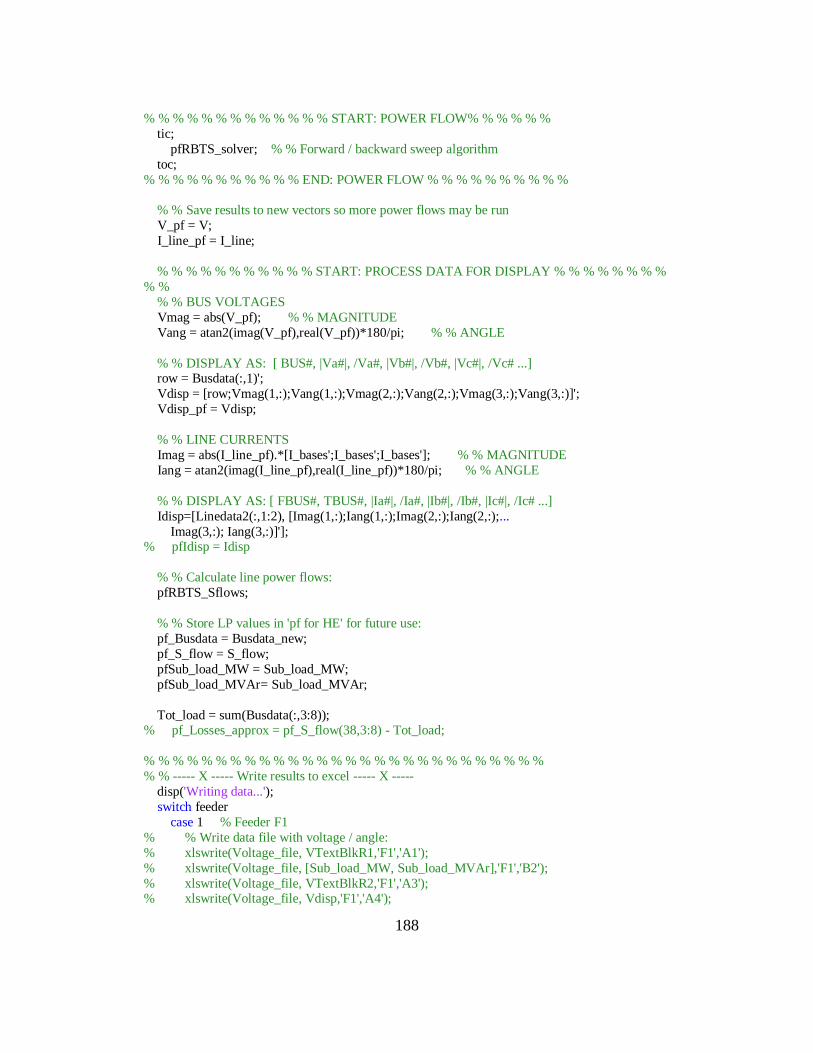
188
% % % % % % % % % % % % % START: POWER FLOW% % % % % %
tic;
pfRBTS_solver; % % Forward / backward sweep algorithm
toc;
% % % % % % % % % % % END: POWER FLOW % % % % % % % % % %
% % Save results to new vectors so more power flows may be run
V_pf = V;
I_line_pf = I_line;
% % % % % % % % % % % START: PROCESS DATA FOR DISPLAY % % % % % % % %
% %
% % BUS VOLTAGES
Vmag = abs(V_pf); % % MAGNITUDE
Vang = atan2(imag(V_pf),real(V_pf))*180/pi; % % ANGLE
% % DISPLAY AS: [ BUS#, |Va#|, /Va#, |Vb#|, /Vb#, |Vc#|, /Vc# ...] row = Busdata(:,1)';
Vdisp = [row;Vmag(1,:);Vang(1,:);Vmag(2,:);Vang(2,:);Vmag(3,:);Vang(3,:)]';
Vdisp_pf = Vdisp;
% % LINE CURRENTS
Imag = abs(I_line_pf).*[I_bases';I_bases';I_bases']; % % MAGNITUDE
Iang = atan2(imag(I_line_pf),real(I_line_pf))*180/pi; % % ANGLE
% % DISPLAY AS: [ FBUS#, TBUS#, |Ia#|, /Ia#, |Ib#|, /Ib#, |Ic#|, /Ic# ...]
Idisp=[Linedata2(:,1:2), [Imag(1,:);Iang(1,:);Imag(2,:);Iang(2,:);...
Imag(3,:); Iang(3,:)]']; % pfIdisp = Idisp
% % Calculate line power flows:
pfRBTS_Sflows;
% % Store LP values in 'pf for HE' for future use:
pf_Busdata = Busdata_new;
pf_S_flow = S_flow;
pfSub_load_MW = Sub_load_MW;
pfSub_load_MVAr= Sub_load_MVAr;
Tot_load = sum(Busdata(:,3:8)); % pf_Losses_approx = pf_S_flow(38,3:8) - Tot_load;
% % % % % % % % % % % % % % % % % % % % % % % % % % % %
% % ----- X ----- Write results to excel ----- X -----
disp('Writing data...');
switch feeder
case 1 % Feeder F1
% % Write data file with voltage / angle:
% xlswrite(Voltage_file, VTextBlkR1,'F1','A1');
% xlswrite(Voltage_file, [Sub_load_MW, Sub_load_MVAr],'F1','B2');
% xlswrite(Voltage_file, VTextBlkR2,'F1','A3'); % xlswrite(Voltage_file, Vdisp,'F1','A4');

189
% % % Write data file with current / angle:%
% xlswrite(Current_file, VTextBlkR1,'F1','A1');
% xlswrite(Current_file, ITextBlkR2,'F1','A2');
% xlswrite(Current_file, Idisp,'F1','A3');
% % % Write data file with power flows:
% xlswrite(Power_file, PTextBlkR1,'F1','A1'); % xlswrite(Power_file, pf_S_flow,'F1','A2');
%
% % % % % % % % % % % % % % % % % % % % % % % % % % % % % % % % % %
%
% case 2 % Feeder F2
% % Write data file with voltage / angle:
% xlswrite(Voltage_file, VTextBlkR1,'F2','A1');
% xlswrite(Voltage_file, [Sub_load_MW, Sub_load_MVAr],'F2','B2');
% xlswrite(Voltage_file, VTextBlkR2,'F2','A3');
% xlswrite(Voltage_file, Vdisp,'F2','A4');
% % % Write data file with current / angle:
% xlswrite(Current_file, VTextBlkR1,'F2','A1'); % xlswrite(Current_file, ITextBlkR2,'F2','A2');
% xlswrite(Current_file, Idisp,'F2','A3');
% % % Write data file with power flows:
% xlswrite(Power_file, PTextBlkR1,'F2','A1');
% xlswrite(Power_file, pf_S_flow,'F2','A2');
%
% % % % % % % % % % % % % %% % % % % % % %% % % % % % %% % % % %
% case 3 % Feeder F3
% % Write data file with busdata and linedata:
% xlswrite(Voltage_file, VTextBlkR1,'F3','A1');
% xlswrite(Voltage_file, [Sub_load_MW, Sub_load_MVAr],'F3','B2'); % xlswrite(Voltage_file, VTextBlkR2,'F3','A3');
% xlswrite(Voltage_file, Vdisp,'F3','A4');
% % % Write data file with busdata and linedata:
% xlswrite(Current_file, VTextBlkR1,'F3','A1');
% xlswrite(Current_file, ITextBlkR2,'F3','A2');
% xlswrite(Current_file, Idisp,'F3','A3');
% % % Write data file with power flows:
% xlswrite(Power_file, PTextBlkR1,'F3','A1');
% xlswrite(Power_file, pf_S_flow,'F3','A2');
%
% % % % % % % % % % % % % %% % % % % % % %% % % % % % %% % % % %
% case 4 % Feeder F4 % % Write data file with busdata and linedata:
% xlswrite(Voltage_file, VTextBlkR1,'F4','A1');
% xlswrite(Voltage_file, [Sub_load_MW, Sub_load_MVAr],'F4','B2');
% xlswrite(Voltage_file, VTextBlkR2,'F4','A3');
% xlswrite(Voltage_file, Vdisp,'F4','A4');
% % % Write data file with busdata and linedata:
% xlswrite(Current_file, VTextBlkR1,'F4','A1');
% xlswrite(Current_file, ITextBlkR2,'F4','A2');
% xlswrite(Current_file, Idisp,'F4','A3');
% % % Write data file with power flows:
% xlswrite(Power_file, PTextBlkR1,'F4','A1'); % xlswrite(Power_file, pf_S_flow,'F4','A2');

190
%
% % % % % % % % % % % % % %% % % % % % % %% % % % % % %% % % % %
% case 5 % Feeder F6
% % Write data file with busdata and linedata:
% xlswrite(Voltage_file, VTextBlkR1,'F6','A1');
% xlswrite(Voltage_file, [Sub_load_MW, Sub_load_MVAr],'F6','B2'); % xlswrite(Voltage_file, VTextBlkR2,'F6','A3');
% xlswrite(Voltage_file, Vdisp,'F6','A4');
% % % Write data file with busdata and linedata:
% xlswrite(Current_file, VTextBlkR1,'F6','A1');
% xlswrite(Current_file, ITextBlkR2,'F6','A2');
% xlswrite(Current_file, Idisp,'F6','A3');
% % % Write data file with power flows:
% xlswrite(Power_file, PTextBlkR1,'F6','A1');
% xlswrite(Power_file, pf_S_flow,'F6','A2');
end
disp('Done writing data...');
% % ======== -+- ======== -+- ======== -+- ======== -+- ======== % %
% % % % % % % % % % % % STATE ESTIMATION ALGORITHM % % % % % % % % %
% % Build the 3-phase YBUS:
YBUS_3ph;
% % % Test the 3-phase YBUS, YV = I
RBTS_I_calc;
% xlswrite('C:\Users\Haughton\Desktop\Icalc',[real(I_calc),imag(I_calc)],'Icalc6cap3ph');
% xlswrite('C:\Users\Haughton\Desktop\Timeseries_sim',[Vdisp],'V6cap3ph'); % xlswrite('C:\Users\Haughton\Desktop\Timeseries_sim',[Idisp],'I6cap3ph');
pf_tstore_I_calc = I_calc;
disp('Entering the estimation algorithm ... ')
SEMain_RBTS_3ph_DR;
end;
toc;

191
The main steering routine for the state estimation portion of the algorithm is pre-
sented subsequently:
% % DATE CREATED / MODIFIED: JULY. 29nd, 2012
% % NAME: SEMain_RBTS_3ph.m
% % DESCRIPTION: Main steering routine for a 3ph unbalanced state estimation algorithm.
Takes Ybus, estimated voltages at SOME NODES, substation power flows, and calculates loads at
unmeasured buses, then estimates bus voltage magnitudes and angles. Calculates flows then dis-
play/saves data to an external (*.csv or *.xls) file.
% % Mod on Dec 22, 2011:
% % Remove hard-coded Isource, Sum MVA and meas MVA. Replace these values
% % with (a) read_timeloads, (b) pf_radial_solver, then calculate I_calc
% % using (c) pf_I_calc to obtain the new Isource values.
% % ------- % ------- % ------- % ------- % ------- % ------- % ------- clear V_mSE I_line_mSE Vmag_mSE Vang_mSE Vdisp_mSE Imag_mSE Iang_mSE...
Idisp_mSE S_flow S_flow_SE Vm_mSE Isource SE_Busdata SE_S_flow...
SESub_load_MW SESub_load_MVAr
%%%%%%%%%%%%%%%%%%%%%%%%%%%%%
Vaccuracy_data = 'C:\Full RBTS Model\LSSSv3\HE 18\Measurement Accuracy.xlsx';
Iaccuracy_data = 'C:\Full RBTS Model\LSSSv3\HE 18\Load Accuracy.xlsx';
[usethis, Volt_meas_var, Load_meas_var] =
Read_meas_data(Vaccuracy_data,Iaccuracy_data,busnos,newbusnos,n_buses,feeder);
% % Demand Response - reduce loads between 5-10(pct).
disp('Demand response - requesting 20% load curtailment');
SE_Demand_Response;
% % Perform power flow with new/modified loads (HE):
pfRBTS_solver;
% % Vector of measurements for SE= XX_mSE:
V_mSE = V;
I_line_mSE = I_line;
% % % % % % % % % % START: PROCESS DATA FOR DISPLAY % % % % % % % % %
% % BUS VOLTAGES Vmag_mSE = abs(V_mSE); % % MAGNITUDE
Vang_mSE = atan2(imag(V_mSE),real(V_mSE))*180/pi; % % ANGLE
% % DISPLAY AS: [ BUS#, |Va#|, /Va#, |Vb#|, /Vb#, |Vc#|, /Vc# ...]
row = Busdata(:,1)';
Vdisp_mSE =[row;Vmag_mSE(1,:);Vang_mSE(1,:);Vmag_mSE(2,:);Vang_mSE(2,:);...
Vmag_mSE(3,:);Vang_mSE(3,:)]';
% % LINE CURRENTS
Imag_mSE = abs(I_line_mSE).*[I_bases';I_bases';I_bases']; % % MAGNITUDE
Iang_mSE = atan2(imag(I_line_mSE),real(I_line_mSE))*180/pi; % % ANGLE
% % DISPLAY AS: [ FBUS#, TBUS#, |Ia#|, /Ia#, |Ib#|, /Ib#, |Ic#|, /Ic# ...]
Idisp_mSE=[Linedata2(:,1:2), [Imag_mSE(1,:);Iang_mSE(1,:);Imag_mSE(2,:);...
Iang_mSE(2,:);Imag_mSE(3,:); Iang_mSE(3,:)]'];

192
% disp('I_disp_mSE'); Idisp_mSE;
% % % % % % % % % % END: PROCESS DATA FOR DISPLAY % % % % % % % % %
% % Calculate line power flows:
pfRBTS_Sflows;
% % Display line power flows S_flow_SE = S_flow;
% % Create a vector, [n_buses*3, 1] by interleaving a, b, c
Vm_mSE(1:3:n_buses*3,1) = V_mSE(1,:);
Vm_mSE(2:3:n_buses*3,1) = V_mSE(2,:);
Vm_mSE(3:3:n_buses*3,1) = V_mSE(3,:);
% % Calculate current injected into source bus:
Isource = Ybus(source_bus*3-2:source_bus*3,:) * Vm_mSE;
% % Store LP values in 'pf for HE' for future use:
SE_Busdata = Busdata_new; SE_S_flow = S_flow;
SESub_load_MW = Sub_load_MW;
SESub_load_MVAr= Sub_load_MVAr;
%%%%%%%%%%%%%%%%%%%%%%%%%%%%%
% % Compare source current to threshhold (1MW here), If dI < I_TH, we
% % will adjust the I_calc vector... ie, Source = Load
SE_Sub_Load_Change;
% % Call the function V_measurements_3ph: Bus voltage measurements are
% % stored in arrays as: V_MEAS_SET# = [BUSno(3x1) ; VOLTAGE(a+jb) ]. % % Note that the BUSno is a 3x1, 3 phases
SE_V_meas_3ph;
%%%%%%%%%%%%%%%%%%%%%%%%%%%%%%%%%%%%%%%%%%
% % Call the function Inj_measurements: % % bus injection currents are
% % stored in arrays as: INJ_MEAS_SET# = [BUS ; CURRENT (a+jb) ]
SE_Inj_meas_3ph;
%%%%%%%%%%%%%%%%%%%%%%%%%%%%%%%%%%%%%%%%%%%%% %
Call the function line_currents: Measurements are provided as
% % I_LINE_MEAS = [FROM BUS; TO BUS ; CURRENT (a+jb) ]
SE_line_currents_3ph;
%%%%%%%%%%%%%%%%%%%%%%%%%%%%%%%%%%%%%%%%%%%%% %
Call the function SE_Algorithm: This builds the x_hat = pinv(H)*z state estimation
tic; % Start recording time
SE_Algorithm_3ph;
toc; % Report run-time
residual = [ (z_s - H_s * x_hat_s), ((z_s - H_s * x_hat_s2).*diag(W))];
J_x = [norm(residual(:,1)); norm(residual(:,2))];
deg_freedom = (n_buses - length(usethis) + n_loadbus_meas)*3 ;
bad_data_limit_99 = chi2inv(0.99,deg_freedom); bad_data_limit_95 = chi2inv(0.95,deg_freedom);

193
bad_data_lim = [bad_data_limit_99; bad_data_limit_95];
% % Calculate power flows:
clear V
for nn = 1:n_buses
V(1:3,nn) = x_hat_s(n_buses*3-2:n_buses*3); end;
pfRBTS_Sflows;
SE_S_flow_result = S_flow;
disp('Writing state estimation results to file'); Voltage_file;
switch feeder
% case 1 % Feeder F1
% % Write data file with voltage / angle:
% xlswrite(Voltage_file, ['J';'J'],'F1_SE','A1');
% xlswrite(Voltage_file, [J_x,bad_data_lim],'F1_SE','B1');
% xlswrite(Voltage_file, VTextBlkR2,'F1_SE','A3');
% xlswrite(Voltage_file, SEVdisp_result,'F1_SE','A4'); % xlswrite(Voltage_file, VTextBlkR2,'F1_SE','I3');
% xlswrite(Voltage_file, WSEVdisp_result,'F1_SE','I4');
case 1 % Feeder F1
xlswrite(Power_file, PTextBlkR1,'F1_SE','A1');
xlswrite(Power_file, SE_S_flow,'F1_SE','A2');
xlswrite(Power_file, PTextBlkR1,'F1_SE','J1');
xlswrite(Power_file, SE_S_flow_result,'F1_SE','J2');
end;