estimation of reliability in multicomponent stress

ProbStat Forum, Volume 05, October 2012, Pages 150–161ISSN 0974-3235

ProbStat Forum is an e-journal.For details please visit www.probstat.org.in

Estimation of reliability in multicomponent stress-strength modelbased on Rayleigh distribution

G. Srinivasa Rao

Department of Statistics, School of Mathematical and Computer Sciences, Dilla University, Ethiopia, P.O. Box: 419

Abstract. A multicomponent system of k components having strengths following k-independentlyand identically distributed random variables and each component experiencing a random stress Y isconsidered. The system is regarded as alive only if at least s out of k (s < k) strengths exceed thestress. The reliability of such a system is obtained when strength, stress variates are given by Rayleighdistribution with different scale parameters. The reliability is estimated using the Moment method andML method of estimation when samples drawn from strength and stress distributions. The reliabilityestimators are compared asymptotically. The small sample comparison of the reliability estimates is madethrough Monte Carlo simulation. Using real data sets we illustrate the procedure.

1. Introduction

The Rayleigh distribution is a special case of the two parameter Weibull distribution and a suitablemodel for life-testing studies. The Rayleigh distribution has the most commonly used distribution in re-liability and life testing (see Lawless (2003)). This distribution has several desirable properties and nicephysical interpretations and it has increasing failure rate. The various applications of this distribution werestudied by Polovko (1968), Gross and Clark (1975), Lee et al. (1980) and Siddiqui (1962). Having founda considerable number of research articles about Rayleigh distribution applications in reliability publishedin various periodicals of wide reputation, we motivated to study the multivariate stress-strength reliabilityestimation based on this distribution. The Rayleigh distribution has the following density function

f(x;σ) =x

σ2e

−x2

2σ2 , x > 0, σ > 0,

and the distribution function

F (x;σ) = 1− e−x2

2σ2 , x > 0, σ > 0,

where X is a continuous random variable defined over (0,∞) and σ is the scale parameter. The purposeof this paper is to study the reliability in a multicomponent stress-strength based on X, Y being twoindependent random variables, where X and Y follows Rayleigh distributions with parameters σ1 and σ2

respectively.

2010 Mathematics Subject Classification. Primary: 62F10; Secondary: 62F12Keywords. Reliability estimation, stress-strength, moment method, ML estimation, confidence intervalsReceived: 06 July 2011; Accepted: 29 June 2012Email address: [email protected] (G. Srinivasa Rao)

Rao / ProbStat Forum, Volume 05, October 2012, Pages 150–161 151

A multicomponent system with k components has strengths following k−independently and identicallydistributed random variables X1, X2, . . . , Xk and each component experiences a random stress Y . Thesystem is regarded as alive only if at least k (s < k) strengths exceed the stress. Let the random samplesY,X1, X2, . . . , Xk be independent, G(y) be the continuous distribution function of Y and F (x) be thecommon continuous distribution function of X1, X2, . . . , Xk. The reliability in a multicomponent stress-strength model developed by Bhattacharyya and Johnson (1974) is given by

Rs,k = P [at least s of the X1, X2, . . . , Xk exceed Y ] =

k∑i=s

(k

i

)∫ ∞−∞

[1−G(y)]i [G(y)](k−i) dF (y), (1)

where X1, X2, . . . , Xk are identically independently distributed (i.i.d.) with common distribution functionF (x) and subjected to the common random stress Y . The probability in (1) is called reliability in amulticomponent stress-strength model (Bhattacharyya and Johnson (1974)). The reliability estimation of asingle component stress-strength version has been considered by several authors assuming various lifetimedistributions for the stress-strength random variates. Enis and Geisser (1971), Downtown (1973), Awadand Gharraf (1986), McCool (1991), Nandi and Aich (1994), Surles and Padgett (1998), Raqab and Kundu(2005), Kundu and Gupta (2005, 2006), Raqab et al. (2008), Kundu and Raqab (2009). The reliability in amulticomponent stress-strength was developed by Bhattacharyya and Johnson (1974), Pandey and Borhan(1985) and the references therein cover the study of estimating P (Y < X) in many standard distributionsassigned to one or both of stress and strength variates. Recently Rao and Kantam (2010) studied estimationof reliability in multicomponent stress-strength for the log-logistic distribution and Rao (2012) developed anestimation of reliability in multicomponent stress-strength based on generalized exponential distribution.

Suppose a system, with k identical components, functions if at least s (1 ≤ s ≤ k) or more of thecomponents simultaneously operate. In its operating environment, the system is subjected to a stress Ywhich is a random variable with distribution function G(·). The strengths of the components, that isthe minimum stresses to cause failure, are independent and identically distributed random variables withdistribution function F (·). Then the system reliability, which is the probability that the system does not fail,is the function Rs,k given in (1). The estimation of survival probability in a multicomponent stress-strengthsystem when the stress and strength variates are following Rayleigh distribution is not paid much attention.Therefore, an attempt is made here to study the estimation of reliability in multicomponent stress-strengthmodel with reference to Rayleigh distribution. The expression for and maximum likelihood (ML) estimatesand Method of Moments (MOM) estimates of the parameters are provided in Section 2. The MOM andMLE are employed to obtain the asymptotic distribution and confidence intervals for Rs,k. The small samplecomparisons made through Monte Carlo simulations in Section 3. Also, using real data, we illustrate theestimation process. Finally, the conclusion and comments are provided in Section 4.

2. Different methods of estimation of parameters in Rs,k

Let X, Y be two independent random variables follows Rayleigh distributions with parameters σ1 andσ2 respectively. The reliability in multicomponent stress-strength for Rayleigh distribution using (1), we get

Rs,k =

k∑i=s

(k

i

)∫ ∞0

[e

−y2

2σ22

]i [1− e

−y2

2σ22

]k−iy

σ21

e−y2

2σ21 dy

=

k∑i=s

(k

i

)∫ 1

0

[tλ2

]i [1− tλ2

]k−idt, where t = e−y2

2σ21 and λ =σ2

1

σ22

=1

λ2

k∑i=s

(k

i

)∫ 1

0

[1− z]k−i [z](1+ 1λ2−1)dz, if z = tλ

2

=1

λ2

k∑i=s

(k

i

)B

(k − i+ 1, i+

1

λ2

).


After the simplification we get

Rs,k =1

λ2

k∑i=s

k!

i!

k∏j=1

(1

λ2− j)

−1

, since k and i are integers. (2)

The probability in (2) is called reliability in a multicomponent stress-strength model. If σ1 and σ2 arenot known, it is necessary to estimate σ1 and σ2 to estimate Rs,k. In this paper we estimate σ1 and σ2

by moment method and ML method. The estimates are substituted in λ to get an estimate of Rs,k usingequation (2). The theory of methods of estimation is explained below.

It is well known that the method of Maximum Likelihood Estimation (MLE) has invariance property.When the method of estimation of parameter is changed from ML to any other traditional method, thisinvariance principle does not hold good to estimate the parametric function. However, such an adoptionof invariance property for other optimal estimators of the parameters to estimate a parametric function isattempted in different situations by different authors. Travadi and Ratani (1990), Kantam and Rao (2002)and the references therein are a few such instances. In this direction, we have proposed some estimators forthe reliability of multicomponent stress-strength model by considering the estimators of the parameters ofstress and strength distributions by ML method and Moment method of estimation in Rayleigh distribution.

2.1. Method of maximum likelihood estimation (MLE)

Let X1, X2, . . . , Xn; Y1, Y2, . . . , Ym be two ordered random samples of size n, m respectively on strengthand stress variates each following Rayleigh distribution with scale parameters σ1 and σ2. The log-likelihoodfunction of the observed sample is

L(σ1, σ2) = −2n lnσ1 − 2m lnσ2 −1

2σ21

n∑i=1

xi −1

2σ22

m∑j=1

yj +

n∑i=1

lnxi +

m∑j=1

ln yj .

The MLEs σ̂1 and σ̂2 of σ1 and σ2 respectively can be obtained as

∂L

∂σ1= 0⇒ σ̂1 =

√√√√ 1

2n

n∑i=1

x2i ,

∂L

∂σ2= 0⇒ σ̂2 =

√√√√ 1

2m

m∑i=1

y2i .

Once we obtain σ̂1 and σ̂2 the ML estimator of Rs,k becomes R̂s,k with λ is replaced by λ̂ in (2).

2.2. Method of moment estimation (MOM)

We know that, if x and y are the sample means of samples on strength and stress variates then moment

estimators of σ1 and σ2 are σ̃1 = x√

2Π and σ̃2 = y

√2Π , respectively. The MOM estimator of Rs,k, we

propose here is R̃s,k with λ is replaced by λ̃ = σ̃1

σ̃2in (2).

To obtain the asymptotic confidence interval for Rs,k, we proceed as follows. The asymptotic varianceof the MLEs are given by

V (σ̂1) =

[E

(−∂

2L

∂σ21

)]−1

=σ2

1

4nand V (σ̂2) =

[E

(−∂

2L

∂σ22

)]−1

=σ2

2

4m.

Under central limit property for i.i.d. variates, the asymptotic distribution of the moment estimators arenormal with the asymptotic variances are given by

V (σ̃1) = V

x√Π2

=

(4−Π

Π

)σ2

1

nand V (σ̃2) = V

y√Π2

=

(4−Π

Π

)σ2

2

m.


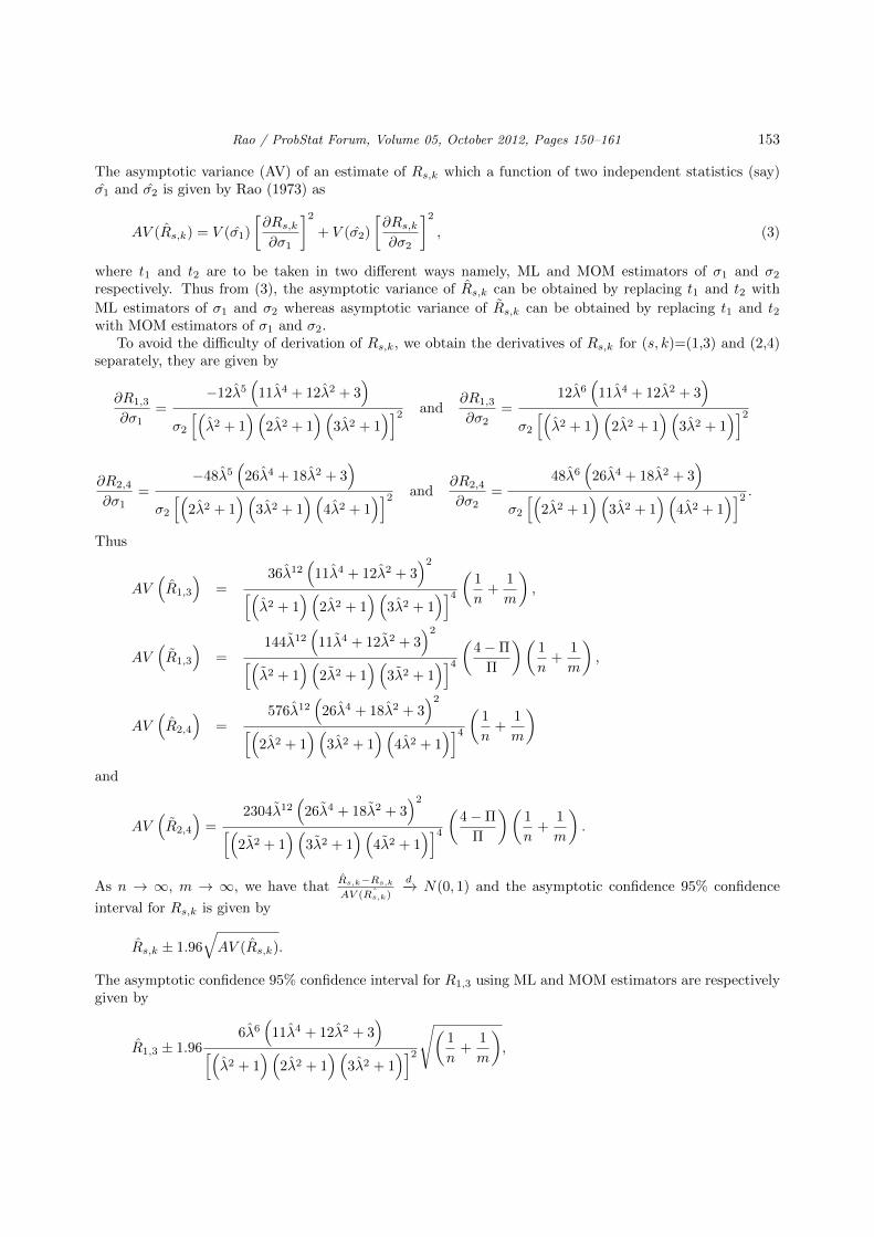
The asymptotic variance (AV) of an estimate of Rs,k which a function of two independent statistics (say)σ̂1 and σ̂2 is given by Rao (1973) as

AV (R̂s,k) = V (σ̂1)

[∂Rs,k∂σ1

]2

+ V (σ̂2)

[∂Rs,k∂σ2

]2

, (3)

where t1 and t2 are to be taken in two different ways namely, ML and MOM estimators of σ1 and σ2

respectively. Thus from (3), the asymptotic variance of R̂s,k can be obtained by replacing t1 and t2 with

ML estimators of σ1 and σ2 whereas asymptotic variance of R̃s,k can be obtained by replacing t1 and t2with MOM estimators of σ1 and σ2.

To avoid the difficulty of derivation of Rs,k, we obtain the derivatives of Rs,k for (s, k)=(1,3) and (2,4)separately, they are given by

∂R1,3

∂σ1=

−12λ̂5(

11λ̂4 + 12λ̂2 + 3)

σ2

[(λ̂2 + 1

)(2λ̂2 + 1

)(3λ̂2 + 1

)]2 and∂R1,3

∂σ2=

12λ̂6(

11λ̂4 + 12λ̂2 + 3)

σ2

[(λ̂2 + 1

)(2λ̂2 + 1

)(3λ̂2 + 1

)]2∂R2,4

∂σ1=

−48λ̂5(

26λ̂4 + 18λ̂2 + 3)

σ2

[(2λ̂2 + 1

)(3λ̂2 + 1

)(4λ̂2 + 1

)]2 and∂R2,4

∂σ2=

48λ̂6(

26λ̂4 + 18λ̂2 + 3)

σ2

[(2λ̂2 + 1

)(3λ̂2 + 1

)(4λ̂2 + 1

)]2 .Thus

AV(R̂1,3

)=

36λ̂12(

11λ̂4 + 12λ̂2 + 3)2

[(λ̂2 + 1

)(2λ̂2 + 1

)(3λ̂2 + 1

)]4 ( 1

n+

1

m

),

AV(R̃1,3

)=

144λ̃12(

11λ̃4 + 12λ̃2 + 3)2

[(λ̃2 + 1

)(2λ̃2 + 1

)(3λ̃2 + 1

)]4 (4−Π

Π

)(1

n+

1

m

),

AV(R̂2,4

)=

576λ̂12(

26λ̂4 + 18λ̂2 + 3)2

[(2λ̂2 + 1

)(3λ̂2 + 1

)(4λ̂2 + 1

)]4 ( 1

n+

1

m

)

and

AV(R̃2,4

)=

2304λ̃12(

26λ̃4 + 18λ̃2 + 3)2

[(2λ̃2 + 1

)(3λ̃2 + 1

)(4λ̃2 + 1

)]4 (4−Π

Π

)(1

n+

1

m

).

As n → ∞, m → ∞, we have thatR̂s,k−Rs,kAV ( ˆRs,k)

d−→ N(0, 1) and the asymptotic confidence 95% confidence

interval for Rs,k is given by

R̂s,k ± 1.96

√AV (R̂s,k).

The asymptotic confidence 95% confidence interval for R1,3 using ML and MOM estimators are respectivelygiven by

R̂1,3 ± 1.966λ̂6

(11λ̂4 + 12λ̂2 + 3

)[(λ̂2 + 1

)(2λ̂2 + 1

)(3λ̂2 + 1

)]2√(

1

n+

1

m

),


R̃1,3 ± 1.9612λ̃6

(11λ̃4 + 12λ̃2 + 3

)[(λ̃2 + 1

)(2λ̃2 + 1

)(3λ̃2 + 1

)]2√(

4−Π

Π

)√(1

n+

1

m

).

The asymptotic confidence 95% confidence interval for R2,4 using ML and MOM estimators are respectivelygiven by

R̂2,4 ± 1.9624λ̂6

(26λ̂4 + 18λ̂2 + 3

)[(

2λ̂2 + 1)(

3λ̂2 + 1)(

4λ̂2 + 1)]2

√(1

n+

1

m

),

R̃2,4 ± 1.9648λ̃6

(26λ̃4 + 18λ̃2 + 3

)[(

2λ̃2 + 1)(

3λ̃2 + 1)(

4λ̃2 + 1)]2

√(4−Π

Π

)√(1

n+

1

m

).

3. Simulation study and data analysis

3.1. Simulation study

In this subsection we present some results based on Monte Carlo simulations to compare the performanceof the Rs,k using for different sample sizes. 3000 random sample of size 10(5)35 each from stress and strengthpopulations are generated for (σ1, σ2)=(3.0, 1.0), (2.5, 1.0), (2.0, 1.0), (1.5, 1.0), (1.0, 1.0), (1.5, 2.0), (1.5,2.5) and (1.5, 3.0) as proposed by Bhattacharyya and Johnson (1974). The ML estimators and MOMestimators of σ1 and σ2 are then substituted in λ to get the reliability in a multicomponent reliability for(s, k) = (1, 3), (2, 4). The average bias and average mean square error (MSE) of the reliability estimates overthe 3000 replications for two methods of estimation are given in Tables 1 and 2. Average confidence lengthand coverage probability of the simulated 95% confidence intervals of Rs,k for two methods of estimationare given in Tables 3 and 4. The true values of reliability in multicomponent stress-strength with the givencombinations of (σ1, σ2) for (s, k) = (1, 3) are 0.178, 0.242, 0.344, 0.507, 0.750, 0.917, 0.971, 0.989, 0.995and for (s, k) = (2, 4) are 0.111, 0.155, 0.228, 0.359, 0.600, 0.828, 0.929, 0.969, 0.986 respectively. Thus thetrue value of reliability in multicomponent stress-strength increases as σ2 increases for a fixed σ1 whereasreliability in multicomponent stress-strength decreases as σ1 increases for a fixed σ2 in both the cases of(s, k). Therefore, the true value of reliability is increases as λ decreases and vice versa. The average bias andaverage MSE are decreases as sample size increases for both methods of estimation in reliability. It verifiesthe consistency property of the MLE of Rs,k. The absolute bias of MLE shows less than the absolute biasof moment estimator in most of the parametric and sample combinations. Also the bias is negative whenσ1 ≤ σ2 and other cases bias is positive in both situations of (s, k). With respect to MSE also MLE showsfirst preference than moment method of estimation. Whereas, among the parameters the absolute bias andMSE are increases as σ1 increases for a fixed value of σ2 in both the cases of (s, k) and the absolute bias andMSE are decreases as σ2 increases for a fixed value of σ1 in both the cases of (s, k). The average length ofthe confidence interval is also decreases as the sample size increases. The average length of the confidenceinterval based on MLE shows shortest average length than by using moment method of estimation. Thesimulated actual coverage probability is close to the nominal value in all cases but slightly less than 0.95in most of the combinations for both methods of estimation. Overall, the performance of the confidenceinterval is quite good for all combinations of parameters. Whereas, among the parameters we observed thesame phenomenon for average length and average simulated actual coverage probability that we observed incase of average bias and MSE. The simulation results also show that there is no considerable difference inthe average bias and average MSE for different choices of the parameters. The same phenomenon is observedfor the average lengths and coverage probabilities of the confidence intervals.


3.2. Data analysis

In this sub section we analyze two real data sets and demonstrate how the proposed methods can be usedin practice. The first data set reported by Wang (2000) and second data set given by Lawless (2003). We fitthe Rayleigh distribution to the two data sets separately. The first data set (Wang (2000)) presented herearose in failure time of 18 devices and they are as follows: Data set I: 5, 11, 21, 31, 46, 75, 98,122, 145,165,195, 224, 245, 293, 321, 330, 350, 420. Wang (2000) has fitted this data to Burr XII distribution. Thesecond data set is obtained from Lawless (2003) and it represents the number of revolution before failureof each of 23 ball bearings in the life tests and they are as follows: Data Set II: 17.88, 28.92, 33.00, 41.52,42.12, 45.60, 48.80, 51.84, 51.96, 54.12, 55.56, 67.80, 68.44, 68.64, 68.88, 84.12, 93.12, 98.64, 105.12, 105.84,127.92, 128.04, 173.40. Gupta and Kundu (2001a) studied the validity of this data for gamma, Weibull andgeneralized exponential distributions.

Before analyzing further, we checked the validity of the models. We used the Kolmogorov-Smirnov(K–S) tests for each data set to fit the Rayleigh distribution. It is observed that for first data set theK–S distance between the empirical distribution function and the fitted distribution functions is 0.22319with the corresponding p– value 0.28647 and for the second data set the K–S distance between the empiricaldistribution function and the fitted distribution functions is 0.14165 with the corresponding p–value 0.69348.It indicates that the Rayleigh model fits quite well to both the data sets. We plot the empirical survivalfunctions and the fitted survival functions in Figures 1 and 2 for data set I and data set II respectively.

The ML and MOM estimates for real data sets are σ̂1 = 137.8, σ̂2 = 57.624 and σ̃1 = 137.25, σ̃2 =57.61, respectively. Basing on ML estimates of σ1 and σ2 the MLE of Rs,k become R̂1,3=0.261981 and

R̂2,4=0.16857. The 95% confidence intervals in this case for R1,3 become (0.131533, 0.392429) and forR2,4 become (0.076964, 0.260176). Similarly, Base on moment estimates of σ1 and σ2 the MOM of Rs,kbecome R̃1,3 = 0.26198 and R̃1,3 = 0.168569. The 95% confidence intervals for R1,3 become (0.125888,0.398072) and for R2,4 become (0.07289, 0.264248). From the real life data, we conclude that one out ofthree component system reliability is more than the two out of four component system reliability for bothmethods of estimation. The length of the confidence interval is also more for one out of three componentsystem reliability than the two out of four component system reliability.

4. Conclusions

In this paper, we have studied the multicomponent stress-strength reliability for Rayleigh distributionwhen both of stress and strength variates follow the same population. Also, we have estimated asymptoticconfidence interval for multicomponent stress-strength reliability using MLE and moment method of estima-tion. The simulation results indicates that the average bias and average MSE are decreases as sample sizeincreases for both methods of estimation in reliability. Among the parameters the absolute bias and MSE areincreases (decreases) as σ1 increases (σ2 increases) in both the cases of (s, k). The length of the confidenceinterval is also decreases as the sample size increases and coverage probability is close to the nominal valuein all sets of parameters considered here. Using real data, we illustrated the estimation process.

Acknowledgement

The author is deeply thankful to the two reviewers and Editor for their valuable suggestions which reallyimprove the quality of the manuscript.

References

Awad, M., Gharraf, K. (1986) Estimation of P (Y < X) in Burr case: A comparative study, Commun. Statist.-Simula. Comp.15, 389–403.

Bhattacharyya, G.K., Johnson, R.A. (1974) Estimation of reliability in multicomponent stress-strength model, JASA 69, 966–970.

Downtown, F. (1973) The estimation of P (Y < X) in the normal case, Technometrics 15 551–558.Enis, P., Geisser, S. (1971) Estimation of the probability that Y < X, JASA 66, 162–168.


Gross, A.J., Clark, V. A. (1975) Survival distributions, Reliability Applications in Biomedical Sciences, Wiley, New York.Gupta, R.D., Kundu, D. (2001a) Generalized exponential distributions; Different Method of Estimations, Journal of Statistical

Computation and Simulation 69, 315–338.Kantam, R.R.L., Rao G.S. (2002) Log-logistic distribution: Modified Maximum likelihood estimation, Gujarat Statistical

Review 29(1-2), 25-36.Kundu, D., Gupta, R.D. (2005) Estimation of P (Y < X) for the generalized exponential distribution, Metrika 61(3), 291–308.Kundu, D., Gupta, R.D. (2006) Estimation of P (Y < X) for Weibull distribution, IEEE Transactions on Reliability 55(2),

270–280.Kundu, D., Raqab, M.Z. (2009) Estimation of R = P (Y < X) for three-parameter Weibull distribution, Statistics and Proba-

bility Letters 79, 1839–1846.Lawless, J.F. (2003) Statistical Models and Methods for Lifetime Data, New York: John Wiley & Sons.Lee. K.R., Kapadia, C.H., Dwigh, B.B. (1980) On estimating the scale parameter of the Rayleigh distribution from doubly

censored samples, Statist. Hefte. 21, 14–29.McCool, J.I. (1991) Inference on P (Y < X) in the Weibull case, Commun. Statist. - Simula. Comp. 20, 129–148.Nandi, S.B., Aich, A.B. (1994) A note on estimation of P (X > Y ) for some distributions useful in life-testing, IAPQR Trans-

actions 19(1), 35–44.Pandey, M., Borhan U.Md. (1985) Estimation of reliability in multicomponent stress-strength model following Burr distribution,

Proceedings of the First Asian congress on Quality and Reliability, New Delhi, India, 307–312.Polovko, A. M. (1968) Fundamentals of Reliability Theory, Academic Press, New York.Rao, C. R. (1973) Linear Statistical Inference and its Applications, Wiley Eastern Limited, India.Rao, G.S. (2012) Estimation of reliability in multicomponent stress-strength model based on generalized exponential distribu-

tion, Colombian Journal of Statistics 35(1), 67–76.Rao, G.S., Kantam, R.R.L. (2010) Estimation of reliability in multicomponent stress-strength model: log-logistic distribution,

Electronic Journal of Applied Statistical Analysis 3(2), 75–84.Raqab, M.Z., Kundu, D. (2005) Comparison of different estimators of P (Y < X) for a scaled Burr type X distribution,

Commun. Statist.-Simula. Comp. 34 (2), 465–483.Raqab, M.Z., Madi, M.T., Kundu, D. (2008) Estimation of P (Y < X) for the 3-parameter generalized exponential distribution,

Commun. Statist-Theor. Meth. 37(18), 2854–2864.Siddiqui, M.M. (1962) Some problems connected with Rayleigh distribution, Journal of Research of the National Bureau of

Standards 66D, 167–174.Surles, J.G., Padgett, W.J. (1998) Inference for P (Y < X) in the Burr type X model, Journal of Applied Statistical Sciences

7, 225–238.Travadi, R.J., Ratani, R.T. (1990) On estimation of reliability function for inverse Guassian distribution with known coefficient

of variation, IAPQR Transactions 5, 29–37.Wang, F.K. (2000) A new model with bathtub-shaped failure rate using an additive Burr XII distribution, Reliability Engi-

neering & Systems Safety 70, 305–312.


Figure 1: The empirical and fitted survival functions for the Data Set I

Figure 2: The empirical and fitted survival functions for the Data Set II


Table 1: Average bias of the simulated estimates of Rs,k

(σ1,σ2)

(s,k) (n,m) (2.5,1.0) (2.0,1.0) (1.5,1.0) (1.0,1.0) (1.0,1.5) (1.0,2.0) (1.0,2.5)

(5,5) 0.02544 0.02161 0.00610 -0.02473 -0.03333 -0.02342 -0.01421

0.02410 0.02072 0.00629 -0.02292 -0.03122 -0.02187 -0.01319

(10,10) 0.01407 0.01290 0.00538 -0.01152 -0.01627 -0.01072 -0.00595

0.01334 0.01229 0.00524 -0.01071 -0.01520 -0.00997 -0.00550

(15,15) 0.00867 0.00753 0.00180 -0.01034 -0.01283 -0.00811 -0.00438

0.00821 0.00726 0.00210 -0.00903 -0.01143 -0.00721 -0.00388

(1,3) (20,20) 0.00728 0.00677 0.00284 -0.00641 -0.00891 -0.00570 -0.00307

0.00586 0.00520 0.00144 -0.00693 -0.00873 -0.00548 -0.00292

(25,25) 0.00739 0.00735 0.00444 -0.00343 -0.00629 -0.00415 -0.00224

0.00665 0.00659 0.00390 -0.00329 -0.00582 -0.00381 -0.00205

(30,30) 0.00434 0.00388 0.00113 -0.00499 -0.00626 -0.00387 -0.00203

0.00381 0.00334 0.00076 -0.00490 -0.00595 -0.00365 -0.00191

(35,35) 0.00314 0.00259 0.00009 -0.00512 -0.00581 -0.00350 -0.00181

0.00302 0.00257 0.00034 -0.00443 -0.00517 -0.00313 -0.00162

(5,5) 0.02357 0.02590 0.02109 -0.00559 -0.03279 -0.03324 -0.02487

0.02212 0.02450 0.02028 -0.00471 -0.03062 -0.03114 -0.02324

(10,10) 0.01226 0.01417 0.01278 -0.00081 -0.01608 -0.01620 -0.01147

0.01159 0.01343 0.01218 -0.00059 -0.01502 -0.01512 -0.01067

(15,15) 0.00773 0.00879 0.00739 -0.00276 -0.01339 -0.01267 -0.00869

0.00726 0.00831 0.00715 -0.00206 -0.01187 -0.01130 -0.00773

(2,4) (20,20) 0.00624 0.00731 0.00672 -0.00051 -0.00893 -0.00885 -0.00612

0.00513 0.00592 0.00513 -0.00165 -0.00908 -0.00863 -0.00588

(25,25) 0.00611 0.00736 0.00738 0.00172 -0.00577 -0.00631 -0.00445

0.00551 0.00663 0.00661 0.00141 -0.00541 -0.00584 -0.00409

(30,30) 0.00379 0.00438 0.00383 -0.00113 -0.00656 -0.00618 -0.00416

0.00336 0.00386 0.00329 -0.00135 -0.00632 -0.00586 -0.00392

(35,35) 0.00283 0.00320 0.00252 -0.00189 -0.00635 -0.00570 -0.00376

0.00269 0.00307 0.00252 -0.00146 -0.00559 -0.00508 -0.00336

In each cell the first row represents the average bias of Rs,k using the MOM and second row represents average bias of Rs,k

using the MLE.


Table 2: Average MSE of the simulated estimates of Rs,k

(σ1,σ2)

(s,k) (n,m) (2.5,1.0) (2.0,1.0) (1.5,1.0) (1.0,1.0) (1.0,1.5) (1.0,2.0) (1.0,2.5)

(5,5) 0.02011 0.02755 0.03330 0.02775 0.01296 0.00516 0.00207

0.01857 0.02576 0.03148 0.02623 0.01202 0.00465 0.00181

(10,10) 0.00929 0.01389 0.01807 0.01446 0.00512 0.00141 0.00037

0.00871 0.01306 0.01704 0.01357 0.00470 0.00126 0.00033

(15,15) 0.00649 0.00991 0.01321 0.01060 0.00353 0.00090 0.00022

0.00591 0.00906 0.01208 0.00960 0.00311 0.00077 0.00019

(1,3) (20,20) 0.00461 0.00721 0.00986 0.00795 0.00252 0.00060 0.00014

0.00415 0.00654 0.00904 0.00735 0.00232 0.00055 0.00013

(25,25) 0.00381 0.00598 0.00817 0.00643 0.00192 0.00043 0.00009

0.00347 0.00546 0.00749 0.00589 0.00173 0.00038 0.00008

(30,30) 0.00303 0.00479 0.00663 0.00529 0.00157 0.00034 0.00007

0.00278 0.00442 0.00615 0.00492 0.00145 0.00031 0.00007

(35,35) 0.00258 0.00411 0.00573 0.00458 0.00132 0.00028 0.00006

0.00234 0.00374 0.00522 0.00416 0.00120 0.00025 0.00005

(5,5) 0.01198 0.01912 0.02888 0.03374 0.02281 0.01191 0.00575

0.01089 0.01762 0.02705 0.03197 0.02146 0.01101 0.00520

(10,10) 0.00494 0.00868 0.01471 0.01853 0.01104 0.00450 0.00161

0.00461 0.00813 0.01384 0.01748 0.01030 0.00412 0.00145

(15,15) 0.00336 0.00603 0.01052 0.01366 0.00798 0.00307 0.00104

0.00305 0.00550 0.00962 0.01247 0.00717 0.00270 0.00089

(2,4) (20,20) 0.00233 0.00427 0.00768 0.01028 0.00591 0.00217 0.00069

0.00208 0.00384 0.00697 0.00946 0.00547 0.00200 0.00063

(25,25) 0.00191 0.00353 0.00637 0.00848 0.00469 0.00164 0.00049

0.00174 0.00321 0.00582 0.00777 0.00428 0.00148 0.00044

(30,30) 0.00151 0.00280 0.00511 0.00693 0.00386 0.00133 0.00040

0.00138 0.00257 0.00472 0.00644 0.00359 0.00123 0.00036

(35,35) 0.00127 0.00238 0.00439 0.00600 0.00332 0.00112 0.00033

0.00115 0.00216 0.00399 0.00547 0.00301 0.00101 0.00029

In each cell the first row represents the average MSE of Rs,k using the MOM and second row represents average MSE of Rs,k

using the MLE.


Table 3: Average confidence length of the simulated 95% confidence intervals of Rs,k

(σ1,σ2)

(s,k) (n,m) (2.5,1.0) (2.0,1.0) (1.5,1.0) (1.0,1.0) (1.0,1.5) (1.0,2.0) (1.0,2.5)

(5,5) 0.51137 0.61702 0.69631 0.62210 0.37763 0.20644 0.11255

0.49107 0.59432 0.67211 0.59907 0.36008 0.19471 0.10505

(10,10) 0.36638 0.45383 0.52420 0.46425 0.26008 0.12784 0.06239

0.35086 0.43538 0.50383 0.44615 0.24848 0.12115 0.05865

(15,15) 0.29764 0.37246 0.43531 0.38721 0.21220 0.10094 0.04771

0.28525 0.35755 0.41859 0.37200 0.20228 0.09526 0.04459

(1,3) (20,20) 0.25870 0.32539 0.38200 0.33830 0.18111 0.08383 0.03865

0.24705 0.31141 0.36661 0.32541 0.17385 0.08012 0.03678

(25,25) 0.23225 0.29264 0.34402 0.30360 0.16015 0.07282 0.03303

0.22215 0.28032 0.33011 0.29156 0.15330 0.06935 0.03130

(30,30) 0.21066 0.26660 0.31531 0.27990 0.14729 0.06646 0.02990

0.20156 0.25534 0.30236 0.26853 0.14099 0.06341 0.02844

(35,35) 0.19466 0.24685 0.29272 0.26029 0.13650 0.06122 0.02737

0.18649 0.23665 0.28080 0.24952 0.13033 0.05817 0.02590

(5,5) 0.37957 0.49543 0.63356 0.70244 0.54478 0.35494 0.21981

0.36291 0.47548 0.61050 0.67812 0.52314 0.33795 0.20745

(10,10) 0.26299 0.35315 0.46760 0.53160 0.39838 0.24122 0.13699

0.25134 0.33807 0.44870 0.51124 0.38233 0.23022 0.12987

(15,15) 0.21131 0.28634 0.38425 0.44345 0.33083 0.19598 0.10832

0.20213 0.27433 0.36895 0.42658 0.31721 0.18656 0.10226

(2,4) (20,20) 0.18255 0.24863 0.33591 0.38939 0.28720 0.16660 0.09003

0.17395 0.23734 0.32156 0.37419 0.27623 0.15985 0.08607

(25,25) 0.16353 0.22312 0.30218 0.35065 0.25670 0.14695 0.07826

0.15619 0.21337 0.28950 0.33671 0.24637 0.14056 0.07454

(30,30) 0.14770 0.20222 0.27543 0.32234 0.23678 0.13503 0.07145

0.14117 0.19345 0.26383 0.30924 0.22707 0.12919 0.06817

(35,35) 0.13619 0.18679 0.25509 0.29959 0.22010 0.12504 0.06583

0.13038 0.17892 0.24457 0.28742 0.21076 0.11930 0.06256

In each cell the first row represents the average confidence length of Rs,k using the MOM and second row represents averageconfidence length of Rs,k using the MLE.


Table 4: Average coverage probability of the simulated 95% confidence intervals of Rs,k

(σ1,σ2)

(s,k) (n,m) (2.5,1.0) (2.0,1.0) (1.5,1.0) (1.0,1.0) (1.0,1.5) (1.0,2.0) (1.0,2.5)

(5,5) 0.9440 0.9483 0.9510 0.9513 0.9400 0.9400 0.9410

0.9417 0.9420 0.9503 0.9533 0.9380 0.9367 0.9380

(10,10) 0.9537 0.9557 0.9533 0.9577 0.9407 0.9370 0.9370

0.9530 0.9523 0.9507 0.9550 0.9407 0.9373 0.9363

(15,15) 0.9440 0.9447 0.9430 0.9480 0.9457 0.9407 0.9403

0.9430 0.9447 0.9427 0.9550 0.9490 0.9423 0.9413

(1,3) (20,20) 0.9513 0.9500 0.9483 0.9477 0.9417 0.9390 0.9377

0.9520 0.9487 0.9487 0.9490 0.9443 0.9397 0.9377

(25,25) 0.9483 0.9493 0.9480 0.9470 0.9473 0.9423 0.9417

0.9497 0.9483 0.9437 0.9453 0.9450 0.9393 0.9373

(30,30) 0.9483 0.9470 0.9483 0.9520 0.9517 0.9460 0.9427

0.9510 0.9500 0.9470 0.9460 0.9507 0.9470 0.9467

(35,35) 0.9490 0.9490 0.9480 0.9517 0.9547 0.9513 0.9487

0.9493 0.9510 0.9500 0.9513 0.9553 0.9513 0.9490

(5,5) 0.9413 0.9437 0.9480 0.9563 0.9460 0.9400 0.9397

0.9397 0.9407 0.9417 0.9550 0.9437 0.9370 0.9363

(10,10) 0.9523 0.9533 0.9557 0.9547 0.9500 0.9397 0.9370

0.9500 0.9523 0.9523 0.9540 0.9497 0.9393 0.9370

(15,15) 0.9470 0.9453 0.9447 0.9433 0.9497 0.9443 0.9403

0.9463 0.9440 0.9450 0.9450 0.9533 0.9477 0.9423

(2,4) (20,20) 0.9533 0.9513 0.9500 0.9490 0.9497 0.9407 0.9387

0.9533 0.9517 0.9490 0.9483 0.9480 0.9427 0.9397

(25,25) 0.9490 0.9473 0.9493 0.9470 0.9480 0.9467 0.9423

0.9480 0.9493 0.9480 0.9430 0.9477 0.9450 0.9393

(30,30) 0.9480 0.9483 0.9463 0.9497 0.9507 0.9497 0.9460

0.9513 0.9510 0.9507 0.9470 0.9483 0.9520 0.9470

(35,35) 0.9490 0.9490 0.9490 0.9493 0.9527 0.9533 0.9513

0.9493 0.9500 0.9510 0.9513 0.9527 0.9547 0.9513

In each cell the first row represents the average coverage probability of Rs,k using the MOM and second row representsaverage coverage probability of Rs,k using the MLE.

estimation of reliability in multicomponent stress

Documents