stat 611 - texas a&m universitycarroll/stat611.directory/call.pdf · stat 611 spring 1998 ......
TRANSCRIPT

STAT 611
R. J. Carroll
January 17, 1999

Contents
1 OFFICE HOURS, etc. 11.1 Office Hours . . . . . . . . . . . . . . . . . . . . . . . . . . . . . . . . . . . . . . . . 11.2 Text . . . . . . . . . . . . . . . . . . . . . . . . . . . . . . . . . . . . . . . . . . . . 11.3 Grading . . . . . . . . . . . . . . . . . . . . . . . . . . . . . . . . . . . . . . . . . . 21.4 About the Instructor . . . . . . . . . . . . . . . . . . . . . . . . . . . . . . . . . . . 2
2 COURSE SCHEDULE 3
3 OLD EXAMS FROM OTHER INSTRUCTORS 53.1 Introduction . . . . . . . . . . . . . . . . . . . . . . . . . . . . . . . . . . . . . . . . 53.2 First Set of Old Exams . . . . . . . . . . . . . . . . . . . . . . . . . . . . . . . . . . 53.3 Second Set of Old Exams . . . . . . . . . . . . . . . . . . . . . . . . . . . . . . . . . 10
4 HOMEWORK ASSIGNMENTS, 1998 134.1 Homework #1 . . . . . . . . . . . . . . . . . . . . . . . . . . . . . . . . . . . . . . . 134.2 Homework #2 . . . . . . . . . . . . . . . . . . . . . . . . . . . . . . . . . . . . . . . 154.3 Homework #3 . . . . . . . . . . . . . . . . . . . . . . . . . . . . . . . . . . . . . . . 164.4 Homework #4 . . . . . . . . . . . . . . . . . . . . . . . . . . . . . . . . . . . . . . . 174.5 Homework #5 . . . . . . . . . . . . . . . . . . . . . . . . . . . . . . . . . . . . . . . 184.6 Homework #6 . . . . . . . . . . . . . . . . . . . . . . . . . . . . . . . . . . . . . . . 204.7 Homework #7 . . . . . . . . . . . . . . . . . . . . . . . . . . . . . . . . . . . . . . . 224.8 Homework #8 . . . . . . . . . . . . . . . . . . . . . . . . . . . . . . . . . . . . . . . 24
5 MY EXAMS FROM 1994 25
6 MY EXAMS FROM 1996 29
7 MY EXAMS FROM 1998 35
8 LECTURE REVIEWS FOR 1996 45
i
Chapter 1
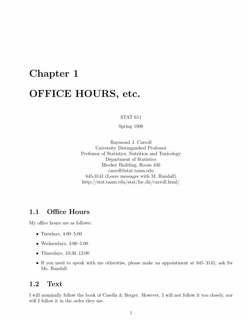
OFFICE HOURS, etc.
STAT 611
Spring 1998
Raymond J. CarrollUniversity Distinguished Professor
Professor of Statistics, Nutrition and ToxicologyDepartment of Statistics
Blocker Building, Room [email protected]
845-3141 (Leave messages with M. Randall)http://stat.tamu.edu/stat/fac.dir/carroll.html/
1.1 Office Hours
My office hours are as follows:
• Tuesdays, 4:00–5:00
• Wednesdays, 3:00–5:00
• Thursdays, 10:30–12:00
• If you need to speak with me otherwise, please make an appointment at 845–3141; ask forMs. Randall.
1.2 Text
I will nominally follow the book of Casella & Berger. However, I will not follow it too closely, norwill I follow it in the order they use.
1
2 CHAPTER 1. OFFICE HOURS, ETC.
1.3 Grading
Homework will count 20% of your final grade. The midterm will count 35%, and the final 45%.The final is cumulative. No late homework assignments will be accepted. I am extremely reluctantto give makeup exams, and will do so only in the most extreme circumstances, e.g. a death in theimmediate family.
For all exams, you may bring six regular sheets of paper filled with whatever notes and formulaeyou think are necessary.
Not all homework problems will be graded. Typically, I will ask the grader to select one problemto grade in detail. The grader will also make up answer sheets. I will give an extra 2% on the finalexam for each mistake you find in the writeup the grader distributes (10 points maximum). Thereis no guarantee that the grader will actually make mistakes!
1.4 About the Instructor
I grew up in D.C., Germany and Wichita Falls, got a B.A. from U.T. Austin in 1971 and a Ph.D.in Statistics from Purdue in 1974. From 1974–1987 I was on the faculty at the University of NorthCarolina at Chapel Hill, also spending time at the Universities of Heidelberg and Wisconsin, aswell as at the National Heart, Lung & Blood Institute. From 1987 to the present I have been afull professor here at A&M, along with having visiting appointments at the Australian NationalUniversity and the National Cancer Institute. I was head of the department from 1987–1990. Icurrently work as a consultant to the National Cancer Institute, and hold two research grants fromthat institute.
My research interests lie in the general area of regression. I wrote a book, Transformation andWeighting in Regression (Chapman & Hall, 1988), which is essentially concerned with heteroscedas-ticity in nonlinear regression. A new book, Measurement Error in Nonlinear Models appeared in1995.
My special interest is nonlinear modeling under unusual error situations. What I try to dois to develop new statistical techniques for solving important practical problems arising out of myconsulting. The techniques I’ve developed have been applied to cancer epidemiology, marine biology,chemometics, pharmacokinetics, marketing, and image processing, among others. The work has wonmy research team a number of awards and honors. I’m currently very interested in the problemsof regression when some of the predictors are measured with error, and my newest techniques arebeing used by cancer epidemiologists in their study of the relationship between breast cancer andnutrition.
My hobbies are trout fishing, golf and cycling.

Chapter 2
COURSE SCHEDULE
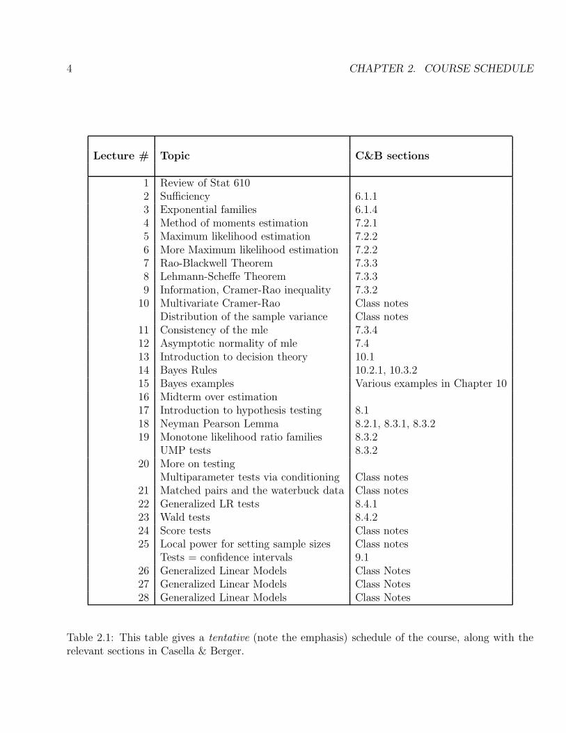
The attached Table 2.1 is tentative, and probably a bit slower than the course will go.The major difference with Casella & Berger is that I will do some multidimensional problems, and
I will do somewhat more with asymptotic theory. Casella & Berger spend an enormous amount oftime on confidence intervals because that is their research interest, but the topic is not of particularimportance for the purpose of this course. I must say that I don’t like many of the things that theydo, and only use the book nominally to save you money.
3
4 CHAPTER 2. COURSE SCHEDULE
Lecture # Topic C&B sections
1 Review of Stat 6102 Sufficiency 6.1.13 Exponential families 6.1.44 Method of moments estimation 7.2.15 Maximum likelihood estimation 7.2.26 More Maximum likelihood estimation 7.2.27 Rao-Blackwell Theorem 7.3.38 Lehmann-Scheffe Theorem 7.3.39 Information, Cramer-Rao inequality 7.3.2
10 Multivariate Cramer-Rao Class notesDistribution of the sample variance Class notes
11 Consistency of the mle 7.3.412 Asymptotic normality of mle 7.413 Introduction to decision theory 10.114 Bayes Rules 10.2.1, 10.3.215 Bayes examples Various examples in Chapter 1016 Midterm over estimation17 Introduction to hypothesis testing 8.118 Neyman Pearson Lemma 8.2.1, 8.3.1, 8.3.219 Monotone likelihood ratio families 8.3.2
UMP tests 8.3.220 More on testing
Multiparameter tests via conditioning Class notes21 Matched pairs and the waterbuck data Class notes22 Generalized LR tests 8.4.123 Wald tests 8.4.224 Score tests Class notes25 Local power for setting sample sizes Class notes
Tests = confidence intervals 9.126 Generalized Linear Models Class Notes27 Generalized Linear Models Class Notes28 Generalized Linear Models Class Notes
Table 2.1: This table gives a tentative (note the emphasis) schedule of the course, along with therelevant sections in Casella & Berger.

Chapter 3
OLD EXAMS FROM OTHERINSTRUCTORS
3.1 Introduction
These are old exams given by other instructors of this course in the recent past. Some of thequestions might be useful to study for qualifying exams.
3.2 First Set of Old Exams
Problem #1. Let X be a random variable with probability density function f(x|θ) given below:
f(x|0) = 1, if 0 ≤ x ≤ 1,
= 0, otherwise,
f(x|1) = 6x(1− x), if 0 ≤ x ≤ 1,
= 0, otherwise,
f(x|2) = 2x, if 0 ≤ x ≤ 1,
= 0, otherwise.
(a.) (18 points) Find the most powerful level 0.1 test of H0 : θ = 0 versus H1 : θ = 1. Obtain itspower.
(b.) (18 points) Is the test obtained in part (b.) the uniformly most powerful level 0.1 test forH0 : θ = 0 versus H1 : θ ∈ 1, 2? Justify your answer.
Note: If you could not find the MP test in part (a.), use the test with rejection region 3, 4 toanswer part (b.).
5

6 CHAPTER 3. OLD EXAMS FROM OTHER INSTRUCTORS
Problem #2. Let X1, . . . , Xm be a random sample from an exponential distribution with density
f(x|θ) =1
θe−x/θ, x > 0.
An important function in reliability and survival analysis is the survival function, S(x) = P[X > x].(a.) (20 points) Obtain the maximum likelihood estimator of the survival function, S(x), for a
specified value xo of x.(b.) (8 points) Derive a lower bound for the variance of unbiased estimators of S(x).(c.) Investigate the limiting distribution of the m.l.e. of S(x).(d.) Obtain the UMVU estimator of S(x). Hint: The conditional density of X1 given
∑ni=1Xi = t
is f(x1|∑Xi = t) = n(t− x1)n−1/tn, 0 < x1 < t.
Problem #3. Let X1, . . . , Xn be independent random variables with cumulative distributionfunction
F (x|θ) = 0, x < 0
= (x
θ)2, 0 ≤ x ≤ θ
= 1, x > θ.
(a.) (18 points) Obtain a pivot based upon the sufficient statistic for θ. Then obtain a 1-αconfidence interval for θ based upon this pivot.
(b.) (18 points) Suppose now that θ is a random variable with prior distribution
π(θ) =1
θ2, θ > 1
= 0, otherwise.
Obtain a 1-α highest posterior density Bayes region for θ.
Problem #4. Let X1, . . . , Xm and Y1, . . . , Yn be independent random samples from normal distri-butions with means µ1 and µ2, respectively, and variances both equal to 1. Obtain the likelihoodratio test of H0 : µ1 = µ2 versus H1 : µ1 6= µ2.
Problem #5. Let X1, . . . , Xn be independent Poisson random variables with probability massfunction
f(x|θ) =e−θθx
x!, x = 0, 1, 2, . . .
Suppose that θ has prior density
π(θ) =1
Γ(α)βαθα−1e−θ/beta, θ > 0.
(a.) Obtain the Bayes estimator of θ with respect to squared error loss.

3.2. FIRST SET OF OLD EXAMS 7
(b) Find the bias, variance and mean squared error of the Bayes estimator. Investigate theconsistency of this estimator.
Problem #6. Let X1, . . . , Xn be a random sample from the distribution with p.d.f.
f(x|θ) = θxθ−1, 0 < x < 1, θ > 0.
(a.) (12 points) Obtain a method of moments estimator of θ.(b.) (12 points) Obtain the maximum likelihood estimator of θ.(c.) (12 points) Obtain the Cramer-Rao lower bound for the variance of unbiased estimators of
θ.(d.) (13 points) Is either of the two above estimators the uniformly minimum variance unbiased
(UMVU) estimator of θ? Justify your answer.
Problem #7. (14 points) Let X1, . . . , Xn be a random sample from the Pareto distribution withdensity
f(x|α, β) =βαβ
xβ+1, α < x <∞, α > 0, β > 0.
Determine whether or not the distribution is of the exponential class. If it is of an exponentialclass, find a complete sufficient statistic. If it is not of exponential class, find a minimal sufficientstatistic.
Problem #8. Let X be a single observation from the N(µ,1) distribution, µ > 0. Notice that theunknown mean is assumed to be positive.
(a.) (12 points) Obtain the UMVU estimator of µ.(b.) (12 points) Obtain the maximum likelihood estimator (MLE) of µ. (Be sure to consider the
parameter space.)(c.) (13 points) Show that the MLE is biased, but has smaller mean squared error than the
UMVUE.
Problem #9. Let X be a random variable with probability mass function f(x|θ) given in thetable.
x = 0 1 2 3 4 5f(x|0) = .1 .2 .3 .1 .1 .2f(x|1) = .3 .1 .1 .2 .1 .2f(x|2) = .2 .2 .1 .1 .3 .1
(a.) (18 points) Find the most powerful level 0.2 test of H0 : θ = 0 versus H1 : θ = 1. Obtain itspower.
(b.) (18 points) Is the test obtained in part (b.) the uniformly most powerful level 0.1 test forH0 : θ = 0 versus H1 : θ ∈ 1, 2? Justify your answer.
8 CHAPTER 3. OLD EXAMS FROM OTHER INSTRUCTORS
Note: If you could not find the MP test in part (a.), use the test with rejection region 3, 4 toanswer part (b.).
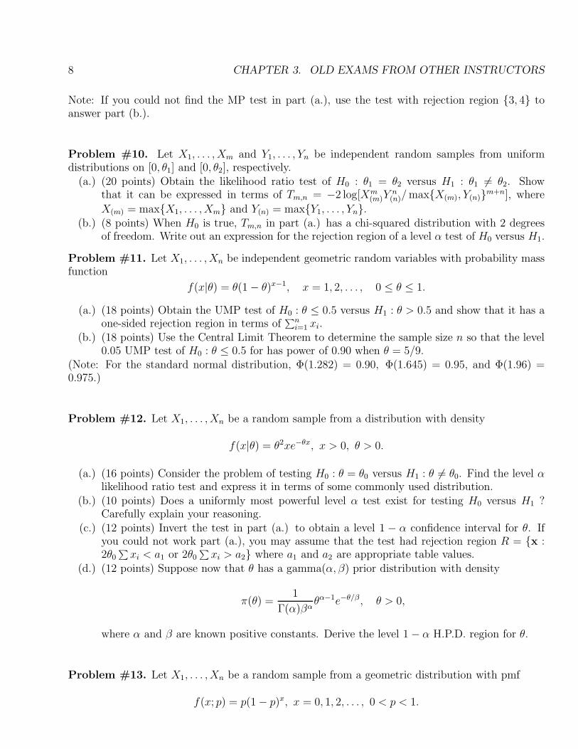
Problem #10. Let X1, . . . , Xm and Y1, . . . , Yn be independent random samples from uniformdistributions on [0, θ1] and [0, θ2], respectively.
(a.) (20 points) Obtain the likelihood ratio test of H0 : θ1 = θ2 versus H1 : θ1 6= θ2. Showthat it can be expressed in terms of Tm,n = −2 log[Xm
(m)Yn
(n)/maxX(m), Y(n)m+n], where
X(m) = maxX1, . . . , Xm and Y(n) = maxY1, . . . , Yn.(b.) (8 points) When H0 is true, Tm,n in part (a.) has a chi-squared distribution with 2 degrees
of freedom. Write out an expression for the rejection region of a level α test of H0 versus H1.
Problem #11. Let X1, . . . , Xn be independent geometric random variables with probability massfunction
f(x|θ) = θ(1− θ)x−1, x = 1, 2, . . . , 0 ≤ θ ≤ 1.
(a.) (18 points) Obtain the UMP test of H0 : θ ≤ 0.5 versus H1 : θ > 0.5 and show that it has aone-sided rejection region in terms of
∑ni=1 xi.
(b.) (18 points) Use the Central Limit Theorem to determine the sample size n so that the level0.05 UMP test of H0 : θ ≤ 0.5 for has power of 0.90 when θ = 5/9.
(Note: For the standard normal distribution, Φ(1.282) = 0.90, Φ(1.645) = 0.95, and Φ(1.96) =0.975.)
Problem #12. Let X1, . . . , Xn be a random sample from a distribution with density
f(x|θ) = θ2xe−θx, x > 0, θ > 0.
(a.) (16 points) Consider the problem of testing H0 : θ = θ0 versus H1 : θ 6= θ0. Find the level αlikelihood ratio test and express it in terms of some commonly used distribution.
(b.) (10 points) Does a uniformly most powerful level α test exist for testing H0 versus H1 ?Carefully explain your reasoning.
(c.) (12 points) Invert the test in part (a.) to obtain a level 1 − α confidence interval for θ. Ifyou could not work part (a.), you may assume that the test had rejection region R = x :2θ0
∑xi < a1 or 2θ0
∑xi > a2 where a1 and a2 are appropriate table values.
(d.) (12 points) Suppose now that θ has a gamma(α, β) prior distribution with density
π(θ) =1
Γ(α)βαθα−1e−θ/β , θ > 0,
where α and β are known positive constants. Derive the level 1− α H.P.D. region for θ.
Problem #13. Let X1, . . . , Xn be a random sample from a geometric distribution with pmf
f(x; p) = p(1− p)x, x = 0, 1, 2, . . . , 0 < p < 1.

3.2. FIRST SET OF OLD EXAMS 9
We are interested in estimating the odds ratio, ξ = (1 − p)/p with squared error loss. To do this,we reparameterize f to obtain the new p.m.f.
f(x; ξ) =ξx
(1 + ξ)1+x, x = 0, 1, 2, . . . , ξ > 0.
(a.) (14 points) Suppose that ξ has a prior distribution of the form
π(ξ) =Γ(α+ β)
Γ(α)Γ(β)
ξα−1
(1 + ξ)(α+β), , ξ > 0,
where α and β are known positive numbers. Show that the Bayes estimator of ξ with respectto π is
Tn =
∑ni=1Xi + α
n+ β − 1.
(b.) (12 points) Obtain the bias and mean squared error of Tn. Hint: Use the results for themean and variance of negative binomial random variables in Casella and Berger. You needto obtain p as a function of ξ.
(c.) (12 points) Investigate the consistency and asymptotic normality of Tn.(d.) (12 points) Obtain Fisher’s information for estimating ξ based on a single observation. Then
determine whether or not Tn is asymptotically efficient.
Problem #14. (12 points each for (a.) and (b.)) For each of the following distributions, letX1, . . . , Xn be a random sample.
(i) State whether or not the distribution is of the exponential class.(ii) If it is of an exponential class, identify c(θ), h(x), w(θ), and t(x) and find the complete
sufficient statistic. If it is not of exponential class, find the minimal sufficient statistic.(a) f(x; θ) = θxθ−1, 0 < x < 1, θ > 0.
(b) f(x; θ) = 3x2
θ3 , 0 < x < θ, θ > 0.
Problem #15. Let X1, . . . , Xn be a random sample from the distribution with density f(x; θ) =θ2xe−θx, x > 0, θ > 0.
(a.) (15 points) Find a method-of-moments estimator of θ. Is it unbiased?(b.) (15 points) Obtain the UMVU estimator of θ.(c.) (15 points) Find the Cramer-Rao Lower Bound on variances of unbiased estimators of θ.
Does the variance of the estimator in (b.) attain the lower bound?
Problem #16. Let X1, . . . , Xn be a random sample from a discrete distribution with pmf f(x; θ) =θ(1− θ)x, x = 0, 1, . . . , 0 < θ < 1.
(a) (15 points) Obtain the maximum likelihood estimator of θ.(b.) (15 points) Obtain the UMVU estimator of θ. Notice that P [X1 = 0] = θ.
10 CHAPTER 3. OLD EXAMS FROM OTHER INSTRUCTORS
Problem #17. Let X be a single observation from a distribution with density %
f(x|θ) = 1, −1 < x < 1, if θ = 0
=3
4(1− x2), −1 < x < 1, if θ = 1.
(a) (20 points) Consider testing H0 : θ = 0 versus H1 : θ = 1. Find the level of significance andpower of the test that has rejection region R = x : |x| > 0.9.
(b) (18 points) Is the test in part (a) the most powerful test of its size for testing H0 versus H1?If it is, prove that it is. If it is not, find the most powerful test.
Problem #18. Let X1, . . . , Xn be a random sample from a Poisson distribution with pmf f(x; θ) =θxe−θ/x!, x = 0, 1, 2, . . . , θ > 0.
(a.) (20 points) Obtain the uniformly most powerful test of its size of H0 : θ ≥ 4 versus H1 : θ < 4.(b.) (18 points) Suppose that n = 100.Use the Central Limit Theorem to obtain an approximately
level .05 test of H0 versus H1. What is the power of this test for the alternative θ = 1? Youmay express your answer in terms of the standard normal distribution function, Φ(x). (Note:Φ(1.645) = .95 and Φ(1.96) = .975.)
Problem #19. (24 points) Let X1, . . . , Xn be a random sample from a normal distribution with
density f(x|µ, σ) = (√
2πσ)−1 exp(−(x−µ)2
2σ2 ). Consider the problem of testing H0 : µ = µ0 versusH1 : µ 6= µ0. Find the level α likelihood ratio test and show that it can be based on the statistic
t =X − µ0
S/√n
where X = n−1∑ni=1Xi and S2 = 1
n−1
∑ni=1(Xi − X)2.
3.3 Second Set of Old Exams
Problem #1. Suppose that X1, . . . , Xn are independent random variables with Xi ∼ Poisson(θ/i),i = 1, . . . , n. The parameter θ is unknown and the parameter space is Θ = (0,∞). For ease ofnotation, define cn =
∑ni=1 i
−1/n.(a) Identify a sufficient statistic and prove that it is sufficient using the factorization theorem.(b) The maximum likelihood estimator of θ is X/cn, where X =
∑ni=1Xi/n. Calculate the mean
squared error of the MLE of θ.
Problem #2. Let X1, . . . , Xn be a random sample from the density
f(x; θ) = θ(1 + x)−(1+θ)I(0,∞)(x), θ > 0.
(a) Assuming that the parameter space is Θ = (1,∞), find a method of moments estimator ofθ. Hint: A useful change of variable in this problem is y = log(1 + x).
3.3. SECOND SET OF OLD EXAMS 11
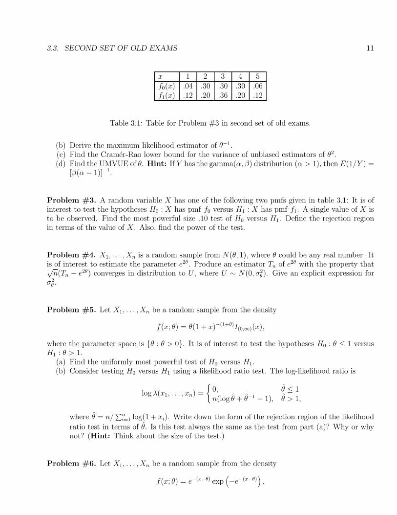
x 1 2 3 4 5f0(x) .04 .30 .30 .30 .06f1(x) .12 .20 .36 .20 .12
Table 3.1: Table for Problem #3 in second set of old exams.
(b) Derive the maximum likelihood estimator of θ−1.(c) Find the Cramer-Rao lower bound for the variance of unbiased estimators of θ2.(d) Find the UMVUE of θ. Hint: If Y has the gamma(α, β) distribution (α > 1), then E(1/Y ) =
[β(α− 1)]−1.
Problem #3. A random variable X has one of the following two pmfs given in table 3.1: It is ofinterest to test the hypotheses H0 : X has pmf f0 versus H1 : X has pmf f1. A single value of X isto be observed. Find the most powerful size .10 test of H0 versus H1. Define the rejection regionin terms of the value of X. Also, find the power of the test.
Problem #4. X1, . . . , Xn is a random sample from N(θ, 1), where θ could be any real number. Itis of interest to estimate the parameter e2θ. Produce an estimator Tn of e2θ with the property that√n(Tn − e2θ) converges in distribution to U , where U ∼ N(0, σ2
θ). Give an explicit expression forσ2θ .
Problem #5. Let X1, . . . , Xn be a random sample from the density
f(x; θ) = θ(1 + x)−(1+θ)I(0,∞)(x),
where the parameter space is θ : θ > 0. It is of interest to test the hypotheses H0 : θ ≤ 1 versusH1 : θ > 1.
(a) Find the uniformly most powerful test of H0 versus H1.(b) Consider testing H0 versus H1 using a likelihood ratio test. The log-likelihood ratio is
log λ(x1, . . . , xn) =
0, θ ≤ 1n(log θ + θ−1 − 1), θ > 1,
where θ = n/∑ni=1 log(1 + xi). Write down the form of the rejection region of the likelihood
ratio test in terms of θ. Is this test always the same as the test from part (a)? Why or whynot? (Hint: Think about the size of the test.)
Problem #6. Let X1, . . . , Xn be a random sample from the density
f(x; θ) = e−(x−θ) exp(−e−(x−θ)
),
12 CHAPTER 3. OLD EXAMS FROM OTHER INSTRUCTORS
where −∞ < θ <∞.(a) (11) Find the Cramer-Rao lower bound for unbiased estimators of θ.(b) (12) Is there a function of θ for which there exists an estimator whose variance coincides
with the Cramer-Rao lower bound? If so, find it.(c) (12) Derive the size α likelihood ratio test of H0 : θ = θ0 versus H1 : θ 6= θ0. Express the
rejection region of the test in terms of a minimal sufficient statistic, and argue that thisregion is the union of two disjoint intervals.
Problem #7. Consider a population with three kinds of individuals labeled 1, 2 and 3 andoccurring in the proportions
f(1; θ) = θ2, f(2; θ) = 2θ(1− θ), f(3; θ) = (1− θ)2,
where 0 < θ < 1. Let X1, . . . , Xn be a random sample from this distribution, and define thestatistics N1, N2, N3 by
Ni = number of Xj′s equal to i, i = 1, 2, 3.
(Note that N1 +N2 +N3 = n.)(a) (6) For any vector (x1, . . . , xn), let ni = the number of xj ’s equal to i, i = 1, 2, 3. Argue that
the joint pmf of X1, . . . , Xn is
f(x1, . . . , xn; θ) =θ2n1 2θ(1− θ)n2 (1− θ)2n3 , each xj = 1, 2, or 30, otherwise.
(b) (11) Prove that 2N1 +N2 is a sufficient statistic.(c) (12) Find the form of the most powerful level α test of
H0 : θ = θ0 versus H1 : θ = 1− θ0,
where θ0 ∈ (0, 1/2). Express the rejection region in terms of n1 and n3.
Problem #8. Consider our old friend from tests I and II, in which X1, . . . , Xn is a random samplefrom the density
f(x; θ) = θ(1 + x)−(1+θ)I(0,∞)(x),
where Θ = (0,∞).(a) (12) Find a pivotal quantity and use it to find a (1− α) confidence interval for θ.
(b) (12) Define θ = n/∑ni=1 log(1 +Xi). Argue that(
1
θ− zα/2
θ√n,
1
θ+zα/2
θ√n
)is an approximate (1−α) confidence interval for 1/θ when n is large, where zp is the (1−p)thquantile of the standard normal distribution.
(c) Now consider a Bayesian approach to estimating θ in the above model. Suppose the priordensity for θ is
π(θ) = e−θI(0,∞)(θ).
Find the posterior density π(θ|x1, . . . , xn) and use it to construct the (1 − α) HPD regionfor θ. You need not obtain the region precisely; just describe how you would obtain it fromπ(θ|x1, . . . , xn).

Chapter 4
HOMEWORK ASSIGNMENTS, 1998
These homeworks may be modified as the semester progresses. It is your responsibility to keep upto date with the correctly assigned homeworks.
There may be some errors in the statements of these problems, due to typographical and con-ceptual errors on my part. I will give 1% addition to the first exam scores for all those findingerrors, under the following conditions: (i) typos are fixed, stated properly and then worked out; (ii)conceptual errors on my part are explained by you.
4.1 Homework #1
Problem #1 Problem 6.1 in Casella & Berger (p. 280).
Problem #2 Problem 6.6 in Casella & Berger (p. 280).
(a) What are the sufficient statistics for α and β?
(b) If α is known, show that the gamma density is a member of the class of exponential families.
(c) If β is known, is the gamma density a member of the class of exponential families? Why orwhy not?
(d) With neither α nor β known, is the gamma density a member of the multiple parameterexponential family? Why or why not?
Problem #3 Suppose that x1, ..., xn are fixed constants. Suppose further that Yi is normallydistributed with mean β0 + β1xi and variance σ2.
(a) What are the sufficient statistics for (β0, β1, σ2)?
Problem #4 The Rayleigh family has the density
f(x, θ) = 2(x/θ2)exp(−x2/θ2
), x > 0, θ > 0.
Use the fact that this is an exponential family to compute the mean, variance and 3rd and 4thmoments of X2, where X is Rayleigh.
13
14 CHAPTER 4. HOMEWORK ASSIGNMENTS, 1998
Problem #5 Suppose I have a sample X1, ..., Xn from the normal distribution with mean θ andvariance θ. Let X be the sample mean, and s2 be the sample variance. Remember that X and s2
are independent.
(a) For any 0 ≤ α ≤ 1, compute the mean and variance of the statistic
T (α) = αX + (1− α)s2.
(b) Compute the limiting distribution of T (α), i.e., what does n1/2T (α) − θ) converge to indistribution.
(c) Is there a unique best value of α as n→∞?
Problem #6 Suppose that we have a sample X1, ..., Xn from the density
f(x, θ) =x!Γ(θ)Γ(x+ θ)
2x+θ.
Find a minimal sufficient statistic for θ.
Problem #7 Work problem 6.20 in Casella and Berger (page 280). A function T (X) is a completesufficient statistic if
E [gT (X)|θ] = 0 for all θ and for all g =⇒ T (X) ≡ 0.
4.2. HOMEWORK #2 15
4.2 Homework #2
Problem #1 Find the mle of θ in the Rayleigh family of Homework #1.
Problem #2 Find the mle’s of (β0, β1, σ2) in the linear regression problem of Homework #1.
Problem #3 Suppose that X1, ..., Xn are a sample with mass function
pr(X = k) =(k − 2)(k − 1)
2(1− θ)k−3θ3.
Find the mle of θ.
Problem #4 Suppose that X1, ..., Xn are i.i.d. uniform on the interval [θ, θ2], where θ > 1.
(a) Show that a method of moments estimator of θ is
θ(MM) =
(
8n−1n∑i=1
Xi + 1
)1/2
− 1
/2.(b) Find the mle for θ.
(c) By combining the central limit theorem and the delta method (Taylor-Slutsky), compute the
limiting distribution of θ(MM).
Problem #5 Work Problem 7.7 in Casella & Berger (page 332).
Problem #6 Work Problem 7.12 of Casella & Berger (page 333).
Problem #7 Suppose that z1, ..., zn are fixed constants, and that the responses Y1, ..., Yn areindependent and normally distributed with mean ziβ and variance σ2v(zi), where v(zi) are knownconstants.
(a) Compute the mle of the parameters.
(b) Compute the mean and variance of β.
Problem #8 Suppose that z1, ..., zn are fixed constants, and that the responses Y1, ..., Yn areindependently distributed according to a gamma distribution with mean exp ziβ and varianceσ2 exp 2ziβ.
(a) It turns out that there is a function ψ(Y, z, β) such that the mle for β solves∑ni=1 ψ(Yi, zi, β) =
0. What is ψ(·)?

16 CHAPTER 4. HOMEWORK ASSIGNMENTS, 1998
4.3 Homework #3
Problem #1 If X ∼ Poisson(θ), show that X is UMVUE for θ.
Problem #2 If X ∼ Binomial(n, θ), show that there exists no unbiased estimator of theodds ratio
g(θ) =θ
1− θ .
HINT: Suppose there does exist an S(X) which is unbiased. Write out EθS(X) and then find acontradiction.
Problem #3 Suppose that X has the mass function
Pr(X = k|θ) = θ(1− θ)k, k = 0, 1, 2, ..../
Find the mle for θ from a sample of size n, and discuss its properties, namely:(a) mean(b) variance(c) is it UMVUE?
Problem #4 Suppose that (z1, ..., zn) are fixed constants, and that for i = 1, ..., n, Xi isnormally distributed with mean zi and variance θz2
i . Find the mle for θ from a sample of size n,and discuss its properties, namely:
(a) mean(b) variance(c) is it UMVUE?HINT: If Z ∼ Normal(0, 1), E(Z3) = 0 and E(Z4) = 3.
Problem #5 Work problem 7.56 in Casella & Berger (page 341).

4.4. HOMEWORK #4 17
4.4 Homework #4
Problem #1 Find the Fisher information for the Rayleigh family.
Problem #2 If X1, ..., Xn are i.i.d. and normally distributed with mean equal to its variance,find the mle and the Fisher information for θ.
Problem #3 Let X be Poisson(λx) and let Y be independent of X and distributed as aPoisson(λy). Define θ = λx/(λx + λy) and ξ = λx + λy.
(a) Suppose that θ is known. Show that T = X + Y is sufficient for ξ.
(b) Compute the conditional distribution of X given T .
(c) Conditioning on T , find the UMVUE for θ. I want you to show that this is really a conditionalUMVUE, so I want you to cite theorems from class to justify your steps.
Problem #4 Suppose I have a sample X1, ..., Xn from the normal distribution with meanθ and variance θ2. Let X be the sample mean, and s2 be the sample variance.
(a) For any 0 ≤ α ≤ 1, compute the mean and variance of the statistic
T (α) = αX2
+ (1− α)s2.
(b) Compute the limiting distribution of T (α).
(c) Compute the limiting distribution of√T (α).
Problem #5 Work Problem 7.55(a) in Casella & Berger (p. 340). Hint #1: An unbiasedestimator is I(X1 = 0), where I(·) is the indicator function. Hint #2: what is the distribution ofX1 given the sufficient statistic?
Problem #6 Suppose that (z1, ..., zn) are fixed constants, and that for i = 1, ..., n, Xi isnormally distributed with mean zi and variance θz2
i . Find the mle for θ from a sample of size n.Does the mle achieve the Fisher information bound? Does this in two ways:
(a) by direct calculation(b) by using properties of OPEF’s.
Problem #7 Suppose that X1, ..., Xn follow the Weibull model with density
f(x|λ, κ) = κλ(λx)κ−1 exp −(λy)κ .
(a) What equations must be solved to compute the mle?

18 CHAPTER 4. HOMEWORK ASSIGNMENTS, 1998
4.5 Homework #5
Problem #1 In the Rayleigh family, show directly using the weak law of large numbers that themle is consistent. Also show it is consistent using the general theory in class about consistency ofmle’s in exponential families.
Problem #2 What is the asymptotic limit distribution of the mle in the Rayleigh family?
Problem #3 Let X1, ..., Xn be i.i.d. negative exponential with mean θ.
(a) Find the mle for θ.
(b) Find the mle for prθ(X > t0).
(c) Prove that the mle for prθ(X > t0) is consistent.
(d) Compute the limit distribution for the mle of prθ(X > t0).
Problem #4 Let X1, ..., Xn be i.i.d. Poisson with mean θ. It moment generating function is knownto be
E exp(tX) = exp [θ exp(t)− 1] .
(a) Show that E(X − θ)2 = θ, E(X − θ)3 = θ and E(X − θ)4 = θ + 3θ2. I may have made anerror here, so correct it if I have.
(b) Compute the limiting distribution for the mle of θ.
(c) The sample variance s2 is unbiased for θ. Compute its limiting distribution.
(d) Compare the limiting variances you found in parts (b) and (c).
Problem #5 Let X1, ..., Xn be i.i.d. from a one parameter exponential family in canonical form,with the density function
p(x|θ) = S(x)exp θx+ d(θ) .
(a) Show that if the mle exists, it must satisfy
X = Eθ(X) |θ=θ
.
(b) Cite a theorem from class showing that the mle must be consistent.
Problem #6 Suppose that X1, ..., Xn follow the Weibull model with density
f(x|λ, κ) = κλ(λx)κ−1 exp −(λy)κ .
(a) Suppose that κ is known. What is the limit distribution for the mle of λ?

4.5. HOMEWORK #5 19
Problem #7 In many problems, time–to–event data would naturally be modeled via a negativeexponential density. However, in some of these problems, there is the “worry” that there is a certainprobability that the event will never occur. Such a model has the distribution (not density) function
Pr(X < x <∞|θ, κ) = (1− κ)1− exp(−x/θ);Pr(X =∞|θ, κ) = κ.
Note that the value of x = ∞ has a positive probability. This model is not in the form of anexponential family, and in fact the data do not even have a density function.
(a) interpret κ as a cure rate.(b) Show that the likelihood function for this model is
κI(x=∞) (1− κ) exp(−x/θ)/θI(x<∞) .
(c) Show that E(X) =∞ and hence standard method of moments will not work.(d) Compute the mle for κ and θ.(e) Compute the limit distribution for the mle of κ.
20 CHAPTER 4. HOMEWORK ASSIGNMENTS, 1998
4.6 Homework #6
Problem #1 Suppose that, given θ, X is Poisson with mean θ. Let θ have a negative exponentialprior distribution with mean θ0. Let the loss function be L(θ, t) = (t− θ)2/θ.
(a) Show that the posterior distribution of θ is a gamma random variable.
(b) What is the Bayes estimator of θ? Hint: you have been told a characterization of Bayesestimators in terms of minimizing a certain function. You should try to do this minimizationexplicitly here.
Problem #2 Let X be Binomial(n, θ1) and let Y be Binomial(n, θ2). Suppose the loss function isL(θ1, θ2, t) = (θ1−θ2−t)2. Let θ1 and θ2 have independent prior beta-distributions with parameters(α, β). Find the Bayes estimator for this loss function.
Problem #3 Work problem 7.24 in Casella & Berger (p. 335).
Problem #4 Let X1, ..., Xn be i.i.d. Normal(0, variance = θ). Suppose I am interested only in thespecial class of estimators of θ defined by
F =
T : Tn(m) = (n+m)−1
n∑i=1
X2i
.
Suppose that the loss function is L(t, θ) = θ−2(t− θ)2.
(a) In this class of estimators, which values of m, if any, yield an admissible estimator?
(b) Is m = 0 minimax?
(c) Answer (a) if the loss function is changed to L(t, θ) = θ−1(t− θ)2.
(c) What is the asymptotic limiting distribution of the mle, in terms of derivatives of the functiond(θ)?
Problem #5 One of the more difficult aspects of Bayesian inference done by frequentists is to finda noninformative prior. Jeffreys’ Prior is the one in which the prior density is proportional to thesquare root of the Fisher information.
Suppose that X1, ..., Xn are independent and identically distributed Bernoulli(θ).(a) Find the Jeffreys prior for this model.
(b) Interpret the Jeffreys prior as a uniform prior for arcsin(√θ).
Problem #6 One criticism of the use of beta priors for Bernoulli sampling is that they are uni-model. Thus, various people have proposed the use of a mixture of betas prior, namely
π(θ) = εgB(θ|a, b) + (1− ε)gB(θ|c, d),
where gB(θ|a, b) is the beta(a, b) density. Show that this prior is conjugate for Bernoulli sampling.
4.6. HOMEWORK #6 21
Problem #7 Suppose that X1, ..., Xn are iid with a negative exponential distribution with mean1/θ.
(a) Find the Jeffreys prior for θ.(b) Compute the posterior distribution for θ.(c) Compute the posterior distribution for λ = 1/θ.(d) Discuss computing the posterior mean and model for λ.

22 CHAPTER 4. HOMEWORK ASSIGNMENTS, 1998
4.7 Homework #7
Problem #1 If X1, ..., Xn are i.i.d. normal with mean θ and variance 1.0, consider testing thehypothesis H0 : θ ≤ 0 against the alternative H1 : θ > 0. What is the power function of the UMPlevel α test?
Problem #2 In Problem #1, suppose that θ has a prior Normal distribution with mean 0.0 andvariance σ2. Consider the 0–1 loss function discussed in class, i.e., the loss is zero if a correctdecision is made, and the loss is one otherwise. What is the Bayes procedure for this problem?
Problem #3 Let X1, ..., Xn be i.i.d. with a common density
p(x|θ) = exp −(x− θ) , x ≥ θ.
Let U = min(X1, ..., Xn).
(a) Show that U and U − (1/n) are (respectively) an mle and a UMVUE for θ.
(b) In testing H0 : θ ≤ θ0 against H1 : θ > θ0 at level α, show that the UMP level α test is ofthe form to reject H0 when U > c.
(c) In part (b), express c as a function of θ0 and α.
(d) In parts (b)–(c), what is the power function for the test?
Problem #4 Suppose that X1, ..., Xn are a sample with mass function
pr(X = k) =(k − 2)(k − 1)
2(1− θ)k−3θ3.
(a) Show that if we wish to test H0 : θ ≤ θ0 against H1 : θ > θ0, find the form of the the UMPtest.
(b) What is the Fisher information and the asymptotic distribution of the mle here?
Problem #5 Let X be a Binomial random variable based on a sample of size n = 10 with successprobability θ. Let S = |X − 5|, and suppose this is all that is observed, i.e., I only observe S, andI cannot observe X. Consider testing H0 : θ ≤ 1/3 or θ ≥ 2/3 against H1 : θ = 1/2. Suppose I usethe test which rejects H0 when S = 0 or S = 1.
(a) What is the distribution of S?
(b) Find the level of this test. Remember to consider carefully what “level” means with thiscomposite hypothesis.
(c) Is the test UMP of its level? Why or why not?
Problem #6 Suppose I take n observations from a multinomial distribution with cell probabilitiesas arranged in Table 4.1, and data as in Table 4.2 I am interested in testing the hypothesisH0 : θyy ≤ θyn against the alternative H0 : θyy > θyn. By thinking carefully, find an appropriate

4.7. HOMEWORK #7 23
Yes NoYes θyy θynNo θny θnn
Table 4.1: Table of probabilities for Problem #7. The θ’s sum to 1.0.
Yes NoYes Nyy Nyn
No Nny Nnn
Table 4.2: Table of probabilities for Problem #7. The N ’s sum to n.
conditional test for this hypothesis. By a “conditional test”, I mean that you should condition onpart or all of the data.
24 CHAPTER 4. HOMEWORK ASSIGNMENTS, 1998
4.8 Homework #8
Problem #1 Let X1, ..., Xn be i.i.d. Poisson(θ). Suppose I want to test the hypothesis H0 : θ = θ0
against the alternative H1 : θ 6= θ0.
(a) What is the form of the GLR test here?
(b) What is the form of the Wald test?
(c) What is the form of the score test?
(d) Prove directly that as n→∞, the score test achieves its nominal level α.
Problem #2 Repeat problem #1 but for the case of sampling from the normal distribution withmean and variance both equal to θ.
Problem #3 Let X be Binomial(n, θ1) and let Y be Binomial(n, θ2). Let S = X + Y .
(a) What is the distribution of X given S? You may find it useful to reparameterize θ1 =1 + exp(−∆)−1 and θ2 = 1 + exp(−∆− η)−1.
(c) Is this distribution a member of the one-parameter exponential family with a monotonelikelihood ratio?
(c) Use the result in (a) to find a UMP conditional test of the hypothesis H0 : θ1 ≤ θ2 againstthe alternative H1 : θ1 > θ2.
(d) What is the conditional Wald test for this problem? This is a one-sided test, and we did notcover one-sided testing in class. I’m asking that you come up with a reasonable guess.
Problem #4 Suppose we are concerned with the lower endpoint of computer generated randomnumbers which purport to be uniform on (0, 1). We have a sample X1, ..., Xn are consider thedensity
f(x, θ) =I(θ ≤ x)
1− θ .
Consider the following observations: (.87, .84, .79, .33, .02, .97, .20, .47, .51, .29, .58, .69). Suppose weadopt a prior distribution with density
π(θ) = (1 + a)(1− θ)a.
(a) What kind of prior beliefs does this prior represent?(b) Compute the posterior density for θ.(c) Plot this posterior density for a few values of a.(d) Compute a 95% credible confidence interval for θ, i.e., one which covers 95% of the posterior
density.
Problem #5 Consider the same model as in problem #4, but this time compute a 95% likelihoodratio confidence interval for θ.
Chapter 5
MY EXAMS FROM 1994
EXAM #1, 1994
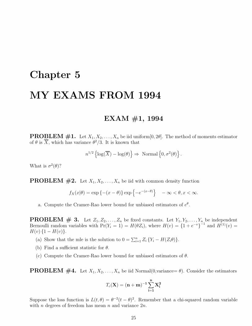
PROBLEM #1. Let X1, X2, . . . , Xn be iid uniform[0, 2θ]. The method of moments estimatorof θ is X, which has variance θ2/3. It is known that
n1/2
log(X)− log(θ)⇒ Normal
0, σ2(θ)
.
What is σ2(θ)?
PROBLEM #2. Let X1, X2, . . . , Xn be iid with common density function
fX(x|θ) = exp −(x− θ) exp−e−(x−θ)
−∞ < θ, x <∞.
a. Compute the Cramer-Rao lower bound for unbiased estimators of eθ.
PROBLEM # 3. Let Z1, Z2, . . . , Zn be fixed constants. Let Y1, Y2, . . . , Yn be independentBernoulli random variables with Pr(Yi = 1) = H(θZi), where H(v) = 1 + e−v−1 and H(1)(v) =H(v) 1−H(v).
(a) Show that the mle is the solution to 0 =∑ni=1 Zi Yi −H(Ziθ).
(b) Find a sufficient statistic for θ.
(c) Compute the Cramer-Rao lower bound for unbiased estimators of θ.
PROBLEM #4. Let X1, X2, . . . , Xn be iid Normal(0,variance= θ). Consider the estimators
Tc(X) = (n + m)−1n∑
i=1
X2i
Suppose the loss function is L(t, θ) = θ−2(t − θ)2. Remember that a chi-squared random variablewith n degrees of freedom has mean n and variance 2n.
25
26 CHAPTER 5. MY EXAMS FROM 1994
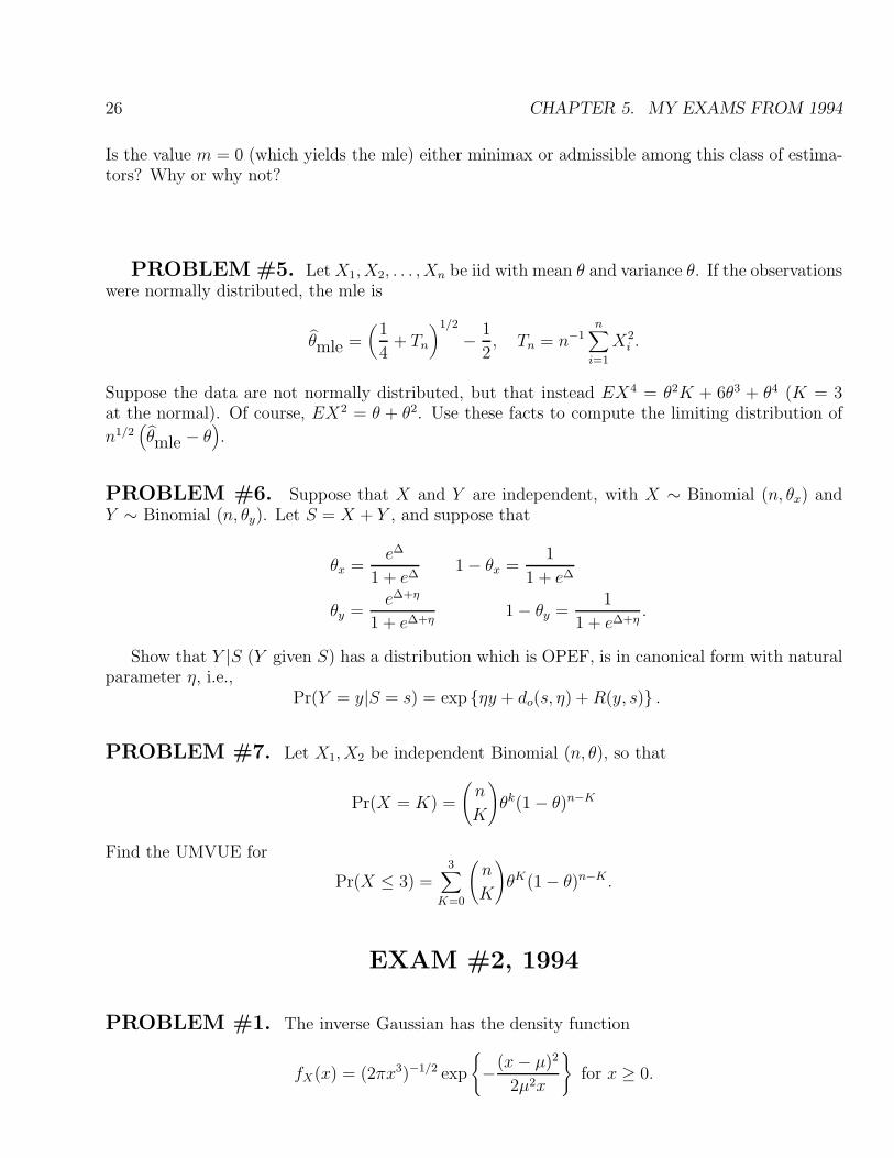
Is the value m = 0 (which yields the mle) either minimax or admissible among this class of estima-tors? Why or why not?
PROBLEM #5. Let X1, X2, . . . , Xn be iid with mean θ and variance θ. If the observationswere normally distributed, the mle is
θmle =(
1
4+ Tn
)1/2
− 1
2, Tn = n−1
n∑i=1
X2i .
Suppose the data are not normally distributed, but that instead EX4 = θ2K + 6θ3 + θ4 (K = 3at the normal). Of course, EX2 = θ + θ2. Use these facts to compute the limiting distribution of
n1/2(θmle − θ
).
PROBLEM #6. Suppose that X and Y are independent, with X ∼ Binomial (n, θx) andY ∼ Binomial (n, θy). Let S = X + Y , and suppose that
θx =e∆
1 + e∆1− θx =
1
1 + e∆
θy =e∆+η
1 + e∆+η1− θy =
1
1 + e∆+η.
Show that Y |S (Y given S) has a distribution which is OPEF, is in canonical form with naturalparameter η, i.e.,
Pr(Y = y|S = s) = exp ηy + do(s, η) +R(y, s) .
PROBLEM #7. Let X1, X2 be independent Binomial (n, θ), so that
Pr(X = K) =
(n
K
)θk(1− θ)n−K
Find the UMVUE for
Pr(X ≤ 3) =3∑
K=0
(n
K
)θK(1− θ)n−K .
EXAM #2, 1994
PROBLEM #1. The inverse Gaussian has the density function
fX(x) = (2πx3)−1/2 exp
−(x− µ)2
2µ2x
for x ≥ 0.

27
(a) Show that E(X) = µ, Var(X) = µ3.
(b) If X1, . . . , Xn are iid, find a conjugate prior for µ.
(c) Suppose you want to test Ω0 : µ ≤ µ0 versus Ω1 : µ > µ0. Citing class results, show thatthe UMP level α test chooses Ω1 when
n−1/2n∑i=1
(Xi − µ0) ≥ c∗,
for some constant c∗.
(d) Indicate in detail how to choose C∗ based on a fixed sample of size n. By “in detail”, I meanthat you must convince me that you can actually get a number within 24 hours.
(e) If n→∞, where does c∗ converge?
(f) What is the level α Wald test for Ω0 : µ = µ0 versus Ω1 : µ 6= µ0?
PROBLEM #2 Let X1, X2, . . . , Xn be iid geometric with
fX(k|θ) = (1− θ)θk k = 0, 1, 2, . . .
E(X|θ) = θ(1− θ)−1 V (X|θ) = θ(1− θ)−2
The prior for θ is Beta (α, β):
π(θ) =θα−1(1− θ)β−1Γα+ β)
Γ(α)Γ(β); Γ(α) = (α− 1)Γ(α− 1).
(a) Find the posterior mean for θ given X = (X1, . . . , Xn).(b) If the loss function is L(t, θ) = (t− θ)2/(1− θ), what is the Bayes estimator of θ?(c) What is the mle of θ? Is there any legitimate choice of (α, β) for which the mle is Bayes in
part (b)?(d) Suppose I have a 0−1 loss function and only two decisions, Ω0 : θ ≤ 1/2 and Ω1 : θ > 1/2.
Describe that the Bayes decision procedure is in this case, in detail.

28 CHAPTER 5. MY EXAMS FROM 1994
Chapter 6
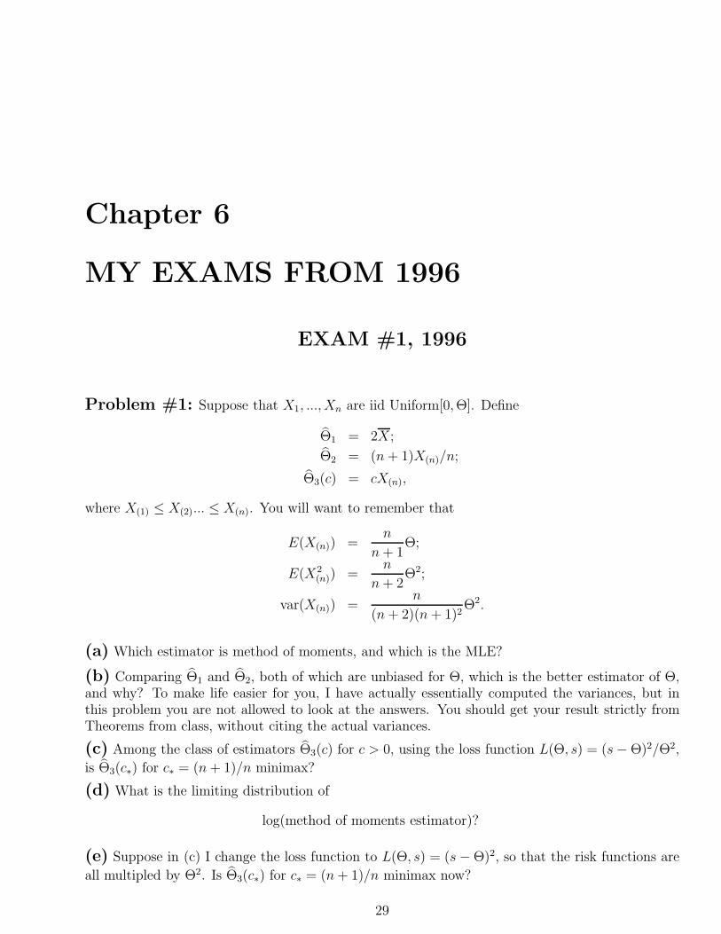
MY EXAMS FROM 1996
EXAM #1, 1996
Problem #1: Suppose that X1, ..., Xn are iid Uniform[0,Θ]. Define
Θ1 = 2X;
Θ2 = (n+ 1)X(n)/n;
Θ3(c) = cX(n),
where X(1) ≤ X(2)... ≤ X(n). You will want to remember that
E(X(n)) =n
n+ 1Θ;
E(X2(n)) =
n
n+ 2Θ2;
var(X(n)) =n
(n+ 2)(n+ 1)2Θ2.
(a) Which estimator is method of moments, and which is the MLE?
(b) Comparing Θ1 and Θ2, both of which are unbiased for Θ, which is the better estimator of Θ,and why? To make life easier for you, I have actually essentially computed the variances, but inthis problem you are not allowed to look at the answers. You should get your result strictly fromTheorems from class, without citing the actual variances.
(c) Among the class of estimators Θ3(c) for c > 0, using the loss function L(Θ, s) = (s−Θ)2/Θ2,
is Θ3(c∗) for c∗ = (n+ 1)/n minimax?
(d) What is the limiting distribution of
log(method of moments estimator)?
(e) Suppose in (c) I change the loss function to L(Θ, s) = (s−Θ)2, so that the risk functions are
all multipled by Θ2. Is Θ3(c∗) for c∗ = (n+ 1)/n minimax now?
29

30 CHAPTER 6. MY EXAMS FROM 1996
Problem #2: Suppose that X1, ..., Xn are iid Beta(Θ,Θ), so that for 0 < x < 1,
f(x|Θ) = xΘ−1(1− x)Θ−1Γ(2Θ)/Γ2(Θ).
Here are some facts (X is the sample mean and s2 is the sample variance):
EΘ(X) = 1/2 for all Θ;
varΘ(X) = 4(2Θ + 1)−1 ;
EΘ(s2) = 4(2Θ + 1)−1 ;
varΘ(s2) = (κ/n) (exact value of κ not important) .
You may assume that the gamma function Γ(s) has first derivative Γ(1)(s) and second derivativeΓ(2)(s), which are otherwise unspecified.
(a) Compute the sufficient statistics for Θ. Cite the Theorem in class which assures you it issufficient.
(b) Compute the Cramer-Rao lower bound for estimating Θ.
(c) Is the MLE for Θ consistent? Why? Cite and apply Theorems from class.
Problem #3: Consider the same setup as in Problem #2.
(a) What is the limit distribution of the MLE?
(b) Why is it that you cannot use the method of moments as applied to X to estimate Θ?
(c) Apply the method of moments to s2 to get an estimate of Θ.
(d) Compute the limit distribution of the estimator you defined in (c).
Problem #4 (DO NOT WORK): In many regression problems in statistics, it is usefulto change the OPEF family slightly, so that
f(x|Θ) = exp
T (x)Θ + d(Θ)
φ+ S(x)
.
Compute E T (X) and var T (X) in terms of Θ and φ. Hint: compute the mgf of T (X), andremember that for all Θ,
1 =∫f(x|Θ)dx
31
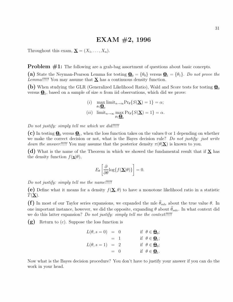
EXAM #2, 1996
Throughout this exam, X = (X1, . . . , Xn).
Problem #1: The following are a grab-bag assortment of questions about basic concepts.
(a) State the Neyman-Pearson Lemma for testing ΘΘΘ0 = θ0 versus ΘΘΘ1 = θ1. Do not prove theLemma!!!!! You may assume that X has a continuous density function.
(b) When studying the GLR (Generalized Likelihood Ratio), Wald and Score tests for testing ΘΘΘ0
versus ΘΘΘ1, based on a sample of size n from iid observations, which did we prove:
(i) maxθ∈ΘΘΘ0
limitn→∞PrθS(X) = 1 = α;
(ii) limitn→∞ maxθ∈ΘΘΘ0
PrθS(X) = 1 = α.
Do not justify: simply tell me which we did!!!!!
(c) In testing ΘΘΘ0 versus ΘΘΘ1, when the loss function takes on the values 0 or 1 depending on whetherwe make the correct decision or not, what is the Bayes decision rule? Do not justify: just writedown the answer!!!!! You may assume that the posterior density π(θ|X) is known to you.
(d) What is the name of the Theorem in which we showed the fundamental result that if X hasthe density function f(x|θ),
Eθ
[∂
∂θlogf(X|θ)
]= 0.
Do not justify: simply tell me the name!!!!!
(e) Define what it means for a density f(X, θ) to have a monotone likelihood ratio in a statisticT (X).
(f) In most of our Taylor series expansions, we expanded the mle θmle about the true value θ. In
one important instance, however, we did the opposite, expanding θ about θmle. In what context didwe do this latter expansion? Do not justify: simply tell me the context!!!!!
(g) Return to (c). Suppose the loss function is
L(θ, s = 0) = 0 if θ ∈ ΘΘΘ0;
= 1 if θ ∈ ΘΘΘ1;
L(θ, s = 1) = 2 if θ ∈ ΘΘΘ0;
= 0 if θ ∈ ΘΘΘ1.
Now what is the Bayes decision procedure? You don’t have to justify your answer if you can do thework in your head.

32 CHAPTER 6. MY EXAMS FROM 1996
Problem #2: On your last exam, many of you had a problem with non–trivial applicationof the delta-method (Taylor–Slutsky). This is a reprise of that problem. Suppose that we havestatistics Tn(X) with the property that
n1/2Tn(X)− (4θ + 1)−1
⇒ Normal(0, κ2).
What is the limiting distribution of [1/Tn(X) − 1] /4?
Problem #3: Suppose that X has a continuous!!! density function
f(x|θ) = exp θT (x) + d(θ) +Q(X) .
This is an OPEF in canonial (natural) form, hence has a monotone likelihood ratio, etc. At leasttwice during the course of the semester I left you a very broad hint that the following problem wascoming.
(a) For arbitrary θ∗ > θ∗∗, in terms of T (X), what is the form of the Neyman-Pearson testΘΘΘ0 = θ∗ versus ΘΘΘ1 = θ∗∗? Simply write this down, but do not derive it!!!!!!
(b) Suppose you are testing ΘΘΘ0 = θ ≥ θ0 against ΘΘΘ1 = θ < θ0. Remember that this is acontinuous density function. What is the form of the UMP level–α test? Simply write this down,but do not derive it!!!!!!
(c) Show that the power function of the test in (b) is monotone nonincreasing. Provide a formalproof based upon contradiction, using (a). Remember that this is a problem with a continuousdensity function.
33
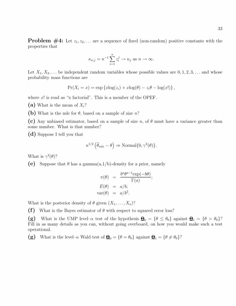
Problem #4: Let z1, z2, . . . are a sequence of fixed (non-random) positive constants with theproperties that
κn,j = n−1n∑i=1
zji → κj as n→∞.
Let X1, X2, . . . be independent random variables whose possible values are 0, 1, 2, 3, . . . and whoseprobability mass functions are
Pr(Xi = x) = exp xlog(zi) + xlog(θ)− ziθ − log(x!) ,
where x! is read as “x factorial”. This is a member of the OPEF.
(a) What is the mean of Xi?
(b) What is the mle for θ, based on a sample of size n?
(c) Any unbiased estimator, based on a sample of size n, of θ must have a variance greater thansome number. What is that number?
(d) Suppose I tell you that
n1/2(θmle − θ
)⇒ Normal0, γ2(θ).
What is γ2(θ)?
(e) Suppose that θ has a gamma(a,1/b)-density for a prior, namely
π(θ) =baθa−1exp(−bθ)
Γ(a);
E(θ) = a/b;
var(θ) = a/b2.
What is the posterior density of θ given (X1, . . . , Xn)?
(f) What is the Bayes estimator of θ with respect to squared error loss?
(g) What is the UMP level–α test of the hypothesis ΘΘΘ0 = θ ≤ θ0 against ΘΘΘ1 = θ > θ0?Fill in as many details as you can, without going overboard, on how you would make such a testoperational.
(g) What is the level–α Wald test of ΘΘΘ0 = θ = θ0 against ΘΘΘ1 = θ 6= θ0?

34 CHAPTER 6. MY EXAMS FROM 1996
Chapter 7
MY EXAMS FROM 1998
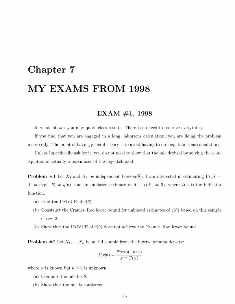
EXAM #1, 1998
In what follows, you may quote class results. There is no need to rederive everything.
If you find that you are engaged in a long, laborious calculation, you are doing the problem
incorrectly. The point of having general theory is to avoid having to do long, laborious calculations.
Unless I specifically ask for it, you do not need to show that the mle derived by solving the score
equation is actually a maximizer of the log–likelihood.
Problem #1 Let X1 and X2 be independent Poisson(θ). I am interested in estimating Pr(X =
0) = exp(−θ) = q(θ), and an unbiased estimate of it is I(X1 = 0), where I(·) is the indicator
function.
(a) Find the UMVUE of q(θ).
(b) Construct the Cramer–Rao lower bound for unbiased estimates of q(θ) based on this sample
of size 2.
(c) Show that the UMVUE of q(θ) does not achieve the Cramer–Rao lower bound.
Problem #2 Let X1, ..., Xn be an iid sample from the inverse gamma density:
f(x|θ) =θαexp(−θ/x)
xα+1Γ(α),
where α is known but θ > 0 is unknown.
(a) Compute the mle for θ.
(b) Show that the mle is consistent.
35
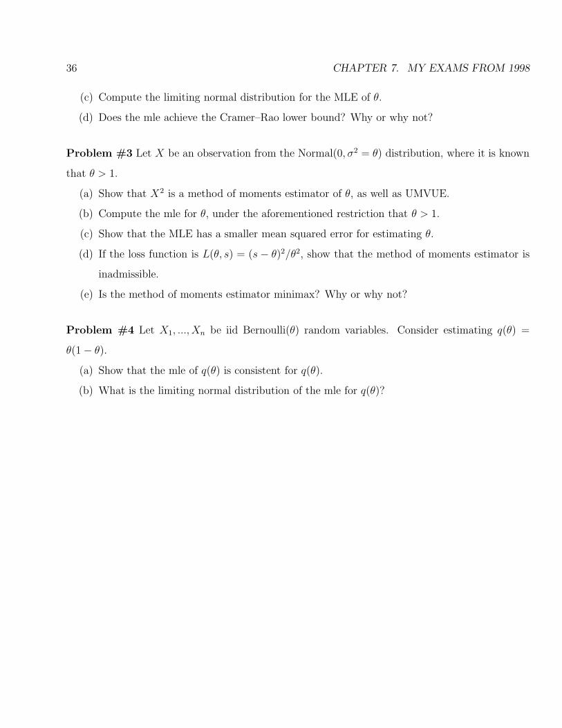
36 CHAPTER 7. MY EXAMS FROM 1998
(c) Compute the limiting normal distribution for the MLE of θ.
(d) Does the mle achieve the Cramer–Rao lower bound? Why or why not?
Problem #3 Let X be an observation from the Normal(0, σ2 = θ) distribution, where it is known
that θ > 1.
(a) Show that X2 is a method of moments estimator of θ, as well as UMVUE.
(b) Compute the mle for θ, under the aforementioned restriction that θ > 1.
(c) Show that the MLE has a smaller mean squared error for estimating θ.
(d) If the loss function is L(θ, s) = (s− θ)2/θ2, show that the method of moments estimator is
inadmissible.
(e) Is the method of moments estimator minimax? Why or why not?
Problem #4 Let X1, ..., Xn be iid Bernoulli(θ) random variables. Consider estimating q(θ) =
θ(1− θ).
(a) Show that the mle of q(θ) is consistent for q(θ).
(b) What is the limiting normal distribution of the mle for q(θ)?
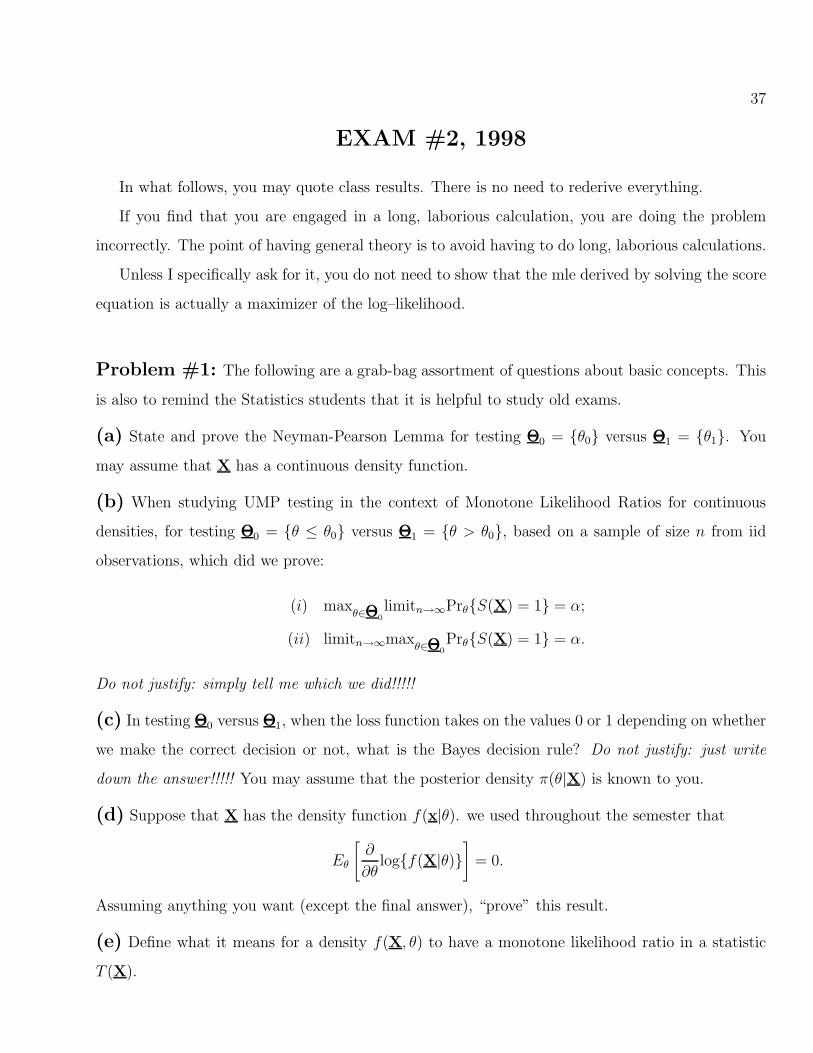
37
EXAM #2, 1998
In what follows, you may quote class results. There is no need to rederive everything.
If you find that you are engaged in a long, laborious calculation, you are doing the problem
incorrectly. The point of having general theory is to avoid having to do long, laborious calculations.
Unless I specifically ask for it, you do not need to show that the mle derived by solving the score
equation is actually a maximizer of the log–likelihood.
Problem #1: The following are a grab-bag assortment of questions about basic concepts. This
is also to remind the Statistics students that it is helpful to study old exams.
(a) State and prove the Neyman-Pearson Lemma for testing ΘΘΘ0 = θ0 versus ΘΘΘ1 = θ1. You
may assume that X has a continuous density function.
(b) When studying UMP testing in the context of Monotone Likelihood Ratios for continuous
densities, for testing ΘΘΘ0 = θ ≤ θ0 versus ΘΘΘ1 = θ > θ0, based on a sample of size n from iid
observations, which did we prove:
(i) maxθ∈ΘΘΘ0
limitn→∞PrθS(X) = 1 = α;
(ii) limitn→∞maxθ∈ΘΘΘ0
PrθS(X) = 1 = α.
Do not justify: simply tell me which we did!!!!!
(c) In testing ΘΘΘ0 versus ΘΘΘ1, when the loss function takes on the values 0 or 1 depending on whether
we make the correct decision or not, what is the Bayes decision rule? Do not justify: just write
down the answer!!!!! You may assume that the posterior density π(θ|X) is known to you.
(d) Suppose that X has the density function f(x|θ). we used throughout the semester that
Eθ
[∂
∂θlogf(X|θ)
]= 0.
Assuming anything you want (except the final answer), “prove” this result.
(e) Define what it means for a density f(X, θ) to have a monotone likelihood ratio in a statistic
T (X).
38 CHAPTER 7. MY EXAMS FROM 1998
Problem #2: Suppose that X1, ..., Xn, ... are iid from a Rayleigh density parameterized in
convenient form as
f(x|η) = 2xηexp(−ηx2).
(a) What is the Fisher information for η in a sample of size n?
(b) What is the mle for η?
(c) What is the limiting distribution for the mle of η, i.e., as n → ∞, what is the distribution of
n1/2(ηmle − η)?
(d) What is the limiting distribution in the sense of (c) for√ηmle?
(e) What is the UMP test for ΘΘΘ0η ≤ η0 versus ΘΘΘ1η > η0? You can use class results, but you
should state them as you go, and please remember to be careful, as this one has somewhat tricky
algebra.
(f) What is the conjugate prior density for η?
(g) Derscribe how you would go about computing a 95% HPD credible region for η. Once you
derive the posterior, you can then just give a brief outline.
(h) Work out as many details as you can of the form of the GLR test of ΘΘΘ0 = η = η0 versus
ΘΘΘ1 = η 6= η0.
(i) What is the Wald test of ΘΘΘ0 = η = η0 versus ΘΘΘ1 = η 6= η0.
(j) What is the score test of ΘΘΘ0 = η = η0 versus ΘΘΘ1 = η 6= η0.

39
Problem #3: Let X1 and X2 be independent Gamma(θ, λ) random variables, each with density
f(x|θ, λ) = λθxθ−1exp(−λx)/Γ(θ).
In this problem, λ is a nuisance (this word is the hint!!!) parameter and θ is the main parameter of
interest. We have dealt with other nuisance parameter problems, e.g., in the waterbuck data.
(a) Show how to get rid of the nuisance parameter in this problem.
(a) What distribution results?
Problem #4: In many regression problems in statistics, it is useful to change the OPEF family
slightly, so that
f(x|Θ) = exp
T (x)Θ + d(Θ)
φ+ S(x)
.
Compute E T (X) and var T (X) in terms of Θ and φ. Hint: compute the mgf of T (X), and
remember that for all Θ,
1 =∫f(x|Θ)dx
40 CHAPTER 7. MY EXAMS FROM 1998
EXAM #2, 1996
Throughout this exam, X = (X1, . . . , Xn).
Problem #1: The following are a grab-bag assortment of questions about basic concepts.
(a) State the Neyman-Pearson Lemma for testing ΘΘΘ0 = θ0 versus ΘΘΘ1 = θ1. Do not prove the
Lemma!!!!! You may assume that X has a continuous density function.
(b) When studying the GLR (Generalized Likelihood Ratio), Wald and Score tests for testing ΘΘΘ0
versus ΘΘΘ1, based on a sample of size n from iid observations, which did we prove:
(i) maxθ∈ΘΘΘ0
limitn→∞PrθS(X) = 1 = α;
(ii) limitn→∞maxθ∈ΘΘΘ0
PrθS(X) = 1 = α.
Do not justify: simply tell me which we did!!!!!
(c) In testing ΘΘΘ0 versus ΘΘΘ1, when the loss function takes on the values 0 or 1 depending on whether
we make the correct decision or not, what is the Bayes decision rule? Do not justify: just write
down the answer!!!!! You may assume that the posterior density π(θ|X) is known to you.
(d) What is the name of the Theorem in which we showed the fundamental result that if X has
the density function f(x|θ),
Eθ
[∂
∂θlogf(X|θ)
]= 0.
Do not justify: simply tell me the name!!!!!
(e) Define what it means for a density f(X, θ) to have a monotone likelihood ratio in a statistic
T (X).
(f) In most of our Taylor series expansions, we expanded the mle θmle about the true value θ. In
one important instance, however, we did the opposite, expanding θ about θmle. In what context did
we do this latter expansion? Do not justify: simply tell me the context!!!!!
(g) Return to (c). Suppose the loss function is
L(θ, s = 0) = 0 if θ ∈ ΘΘΘ0;

41
= 1 if θ ∈ ΘΘΘ1;
L(θ, s = 1) = 2 if θ ∈ ΘΘΘ0;
= 0 if θ ∈ ΘΘΘ1.
Now what is the Bayes decision procedure? You don’t have to justify your answer if you can do the
work in your head.
42 CHAPTER 7. MY EXAMS FROM 1998
Problem #2: On your last exam, many of you had a problem with non–trivial application
of the delta-method (Taylor–Slutsky). This is a reprise of that problem. Suppose that we have
statistics Tn(X) with the property that
n1/2Tn(X)− (4θ + 1)−1
⇒ Normal(0, κ2).
What is the limiting distribution of [1/Tn(X) − 1] /4?
Problem #3: Suppose that X has a continuous!!! density function
f(x|θ) = exp θT (x) + d(θ) +Q(X) .
This is an OPEF in canonial (natural) form, hence has a monotone likelihood ratio, etc. At least
twice during the course of the semester I left you a very broad hint that the following problem was
coming.
(a) For arbitrary θ∗ > θ∗∗, in terms of T (X), what is the form of the Neyman-Pearson test
ΘΘΘ0 = θ∗ versus ΘΘΘ1 = θ∗∗? Simply write this down, but do not derive it!!!!!!
(b) Suppose you are testing ΘΘΘ0 = θ ≥ θ0 against ΘΘΘ1 = θ < θ0. Remember that this is a
continuous density function. What is the form of the UMP level–α test? Simply write this down,
but do not derive it!!!!!!
(c) Show that the power function of the test in (b) is monotone nonincreasing. Provide a formal
proof based upon contradiction, using (a). Remember that this is a problem with a continuous
density function.

43
Problem #4: Let z1, z2, . . . are a sequence of fixed (non-random) positive constants with the
properties that
κn,j = n−1n∑i=1
zji → κj as n→∞.
Let X1, X2, . . . be independent random variables whose possible values are 0, 1, 2, 3, . . . and whose
probability mass functions are
Pr(Xi = x) = exp xlog(zi) + xlog(θ)− ziθ − log(x!) ,
where x! is read as “x factorial”. This is a member of the OPEF.
(a) What is the mean of Xi?
(b) What is the mle for θ, based on a sample of size n?
(c) Any unbiased estimator, based on a sample of size n, of θ must have a variance greater than
some number. What is that number?
(d) Suppose I tell you that
n1/2(θmle − θ
)⇒ Normal0, γ2(θ).
What is γ2(θ)?
(e) Suppose that θ has a gamma(a,1/b)-density for a prior, namely
π(θ) =baθa−1exp(−bθ)
Γ(a);
E(θ) = a/b;
var(θ) = a/b2.
What is the posterior density of θ given (X1, . . . , Xn)?
(f) What is the Bayes estimator of θ with respect to squared error loss?
(g) What is the UMP level–α test of the hypothesis ΘΘΘ0 = θ ≤ θ0 against ΘΘΘ1 = θ > θ0?
Fill in as many details as you can, without going overboard, on how you would make such a test
operational.
(g) What is the level–α Wald test of ΘΘΘ0 = θ = θ0 against ΘΘΘ1 = θ 6= θ0?

44 CHAPTER 7. MY EXAMS FROM 1998
Chapter 8
LECTURE REVIEWS FOR 1996
45
46 CHAPTER 8. LECTURE REVIEWS FOR 1996
LECTURE #1, 1998
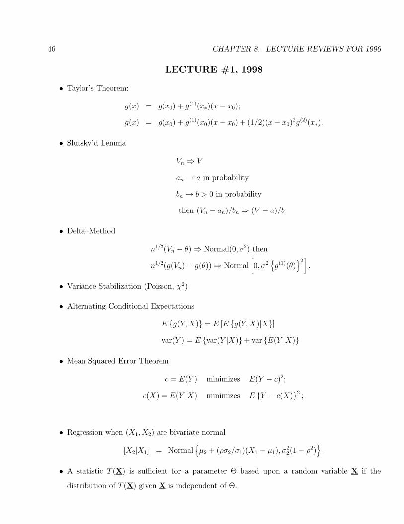
• Taylor’s Theorem:
g(x) = g(x0) + g(1)(x∗)(x− x0);
g(x) = g(x0) + g(1)(x0)(x− x0) + (1/2)(x− x0)2g(2)(x∗).
• Slutsky’d Lemma
Vn ⇒ V
an → a in probability
bn → b > 0 in probability
then (Vn − an)/bn ⇒ (V − a)/b
• Delta–Method
n1/2(Vn − θ)⇒ Normal(0, σ2) then
n1/2(g(Vn)− g(θ))⇒ Normal[0, σ2
g(1)(θ)
2].
• Variance Stabilization (Poisson, χ2)
• Alternating Conditional Expectations
E g(Y,X) = E [E g(Y,X)|X]
var(Y ) = E var(Y |X)+ var E(Y |X)
• Mean Squared Error Theorem
c = E(Y ) minimizes E(Y − c)2;
c(X) = E(Y |X) minimizes E Y − c(X)2 ;
• Regression when (X1, X2) are bivariate normal
[X2|X1] = Normalµ2 + (ρσ2/σ1)(X1 − µ1), σ2
2(1− ρ2).
• A statistic T (X) is sufficient for a parameter Θ based upon a random variable X if the
distribution of T (X) given X is independent of Θ.
47
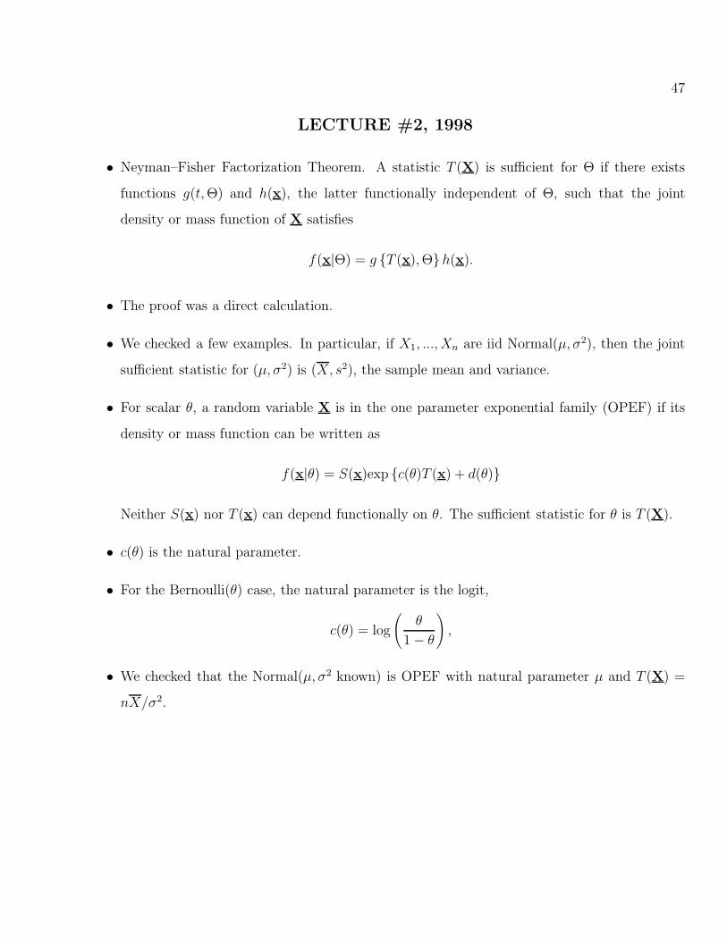
LECTURE #2, 1998
• Neyman–Fisher Factorization Theorem. A statistic T (X) is sufficient for Θ if there exists
functions g(t,Θ) and h(x), the latter functionally independent of Θ, such that the joint
density or mass function of X satisfies
f(x|Θ) = g T (x),Θh(x).
• The proof was a direct calculation.
• We checked a few examples. In particular, if X1, ..., Xn are iid Normal(µ, σ2), then the joint
sufficient statistic for (µ, σ2) is (X, s2), the sample mean and variance.
• For scalar θ, a random variable X is in the one parameter exponential family (OPEF) if its
density or mass function can be written as
f(x|θ) = S(x)exp c(θ)T (x) + d(θ)
Neither S(x) nor T (x) can depend functionally on θ. The sufficient statistic for θ is T (X).
• c(θ) is the natural parameter.
• For the Bernoulli(θ) case, the natural parameter is the logit,
c(θ) = log
(θ
1− θ
),
• We checked that the Normal(µ, σ2 known) is OPEF with natural parameter µ and T (X) =
nX/σ2.
48 CHAPTER 8. LECTURE REVIEWS FOR 1996
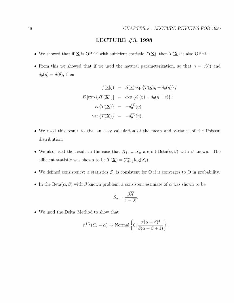
LECTURE #3, 1998
• We showed that if X is OPEF with sufficient statistic T (X), then T (X) is also OPEF.
• From this we showed that if we used the natural parameterization, so that η = c(θ) and
d0(η) = d(θ), then
f(x|η) = S(x)exp T (x)η + d0(η) ;
E [exp sT (X)] = exp d0(η)− d0(η + s) ;
E T (X) = −d(1)0 (η);
var T (X) = −d(2)0 (η);
• We used this result to give an easy calculation of the mean and variance of the Poisson
distribution.
• We also used the result in the case that X1, ..., Xn are iid Beta(α, β) with β known. The
sifficient statistic was shown to be T (X) =∑ni=1 log(Xi).
• We defined consistency: a statistics Sn is consistent for Θ if it converges to Θ in probability.
• In the Beta(α, β) with β known problem, a consistent estimate of α was shown to be
Sn =βX
1−X .
• We used the Delta–Method to show that
n1/2(Sn − α)⇒ Normal
0,
α(α+ β)2
β(α+ β + 1)
.
49
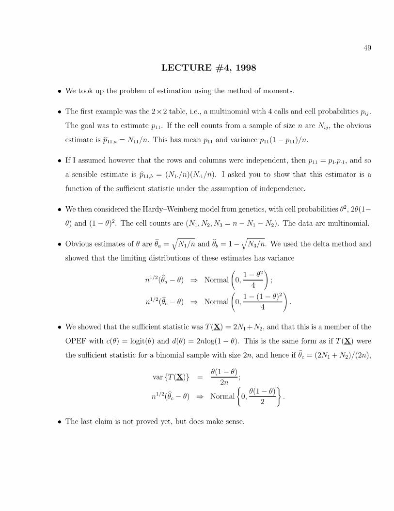
LECTURE #4, 1998
• We took up the problem of estimation using the method of moments.
• The first example was the 2×2 table, i.e., a multinomial with 4 calls and cell probabilities pij .
The goal was to estimate p11. If the cell counts from a sample of size n are Nij , the obvious
estimate is p11,a = N11/n. This has mean p11 and variance p11(1− p11)/n.
• If I assumed however that the rows and columns were independent, then p11 = p1·p·1, and so
a sensible estimate is p11,b = (N1·/n)(N·1/n). I asked you to show that this estimator is a
function of the sufficient statistic under the assumption of independence.
• We then considered the Hardy–Weinberg model from genetics, with cell probabilities θ2, 2θ(1−
θ) and (1− θ)2. The cell counts are (N1, N2, N3 = n−N1 −N2). The data are multinomial.
• Obvious estimates of θ are θa =√N1/n and θb = 1−
√N3/n. We used the delta method and
showed that the limiting distributions of these estimates has variance
n1/2(θa − θ) ⇒ Normal
(0,
1− θ2
4
);
n1/2(θb − θ) ⇒ Normal
(0,
1− (1− θ)2
4
).
• We showed that the sufficient statistic was T (X) = 2N1 +N2, and that this is a member of the
OPEF with c(θ) = logit(θ) and d(θ) = 2nlog(1− θ). This is the same form as if T (X) were
the sufficient statistic for a binomial sample with size 2n, and hence if θc = (2N1 +N2)/(2n),
var T (X) =θ(1− θ)
2n;
n1/2(θc − θ) ⇒ Normal
0,θ(1− θ)
2
.
• The last claim is not proved yet, but does make sense.

50 CHAPTER 8. LECTURE REVIEWS FOR 1996
LECTURE #5, 1998
• We computed the mle for Θ in a number of special cases.
• Normal(µ, σ2)
• Binomial(N, θ), first with θ known (a nonregular family) and then with N known (a regular
family).
• Uniform[0, θ] (a nonregular family)
• Linear regression through the origen.
• We also computed the limiting distribution of s2, i.e., showed that for normally distributed
data, n1/2(s2 − σ2)⇒ Normal(0, 2σ4).
• We write the likelihood as L(X|Θ) and the loglikelihood as `(X|Θ).
• In regular families, one usual maximizes the loglikelihood. Differentiate with respect to the
components of Θ and solve for a zero. This is called an estimating equation. The solution is a
local maximum if the second derivative of the loglikelihood evaluated at the MLE is negative
definite.

51
LECTURE #6, 1998
• We first showed a simple characterization of the MLE in a OPEF: Let c(θ) be 1–1, continuously
differentiable, and suppose that varθT (X) > 0 on the support of X, for all θ. Then if the
MLE exists, it is unique and satisfies
Eθ T (X) = T (X).
• The result was shown in a series of steps:
1. The loglikelihood is ηT (X) + d0(η)+ stuff
2. Its derivative is T (X) + d(1)0 (η)
3. Its second derivative is d(2)0 (η)
4. But we know the mean and variance of T (X) are −d(1)0 (η) and −d(2)
0 (η), respectively.
5. Since the second derivative of the loglikelihood is negative, any solution to the first
equation maximizes the loglikelihood, and there can be only one minimizer.
• We defined the mle of a function g(θ), and showed it to be g(θml
).
• We then began decision theory as a way to compare estimators and to judge their value.
• A loss function for estimating θ by s is L(θ, s)
• The risk function of an estimator S(X) is
R(θ,S) = Eθ [L θ,S(X)] .
• We showed that uniformly best estimators in terms of risk cannot exist. For example, suppose
L(θ, s) = (s−θ)2, and that X ∼ Normal(θ, 1). Then you cannot beat the estimator S(X) = 17
if by chance θ = 17.
52 CHAPTER 8. LECTURE REVIEWS FOR 1996
LECTURE #7, 1998
• An estimator S∗(X) is minimax if
maxθR(θ,S∗) = minS
maxθR(θ,S).
• An estimator S∗(X) is admissible if there exists no other estimator S(X) with the property
that
R(θ,S) ≤ R(θ,S∗) ∀ θ
with at least one strict inequality somewhere.
• Bayes estimators with respect to a prior π(θ) minimize∫R(θ,S)π(θ)dθ. If π(θ) is a density
function, then we can write the conditional density of θ given X as π(θ|X). The Bayes
estimator then minimizes in s
∫L(θ, s)π(θ|X)dθ.
• We considered the case that X ∼ Normal(θ, 1), and looked at the class of estimators cX with
0 < c ≤ 1. We showed that only c = 1 is minimax. I asked you to argue that all values of c
are admissible. I promised that later I would show that only 0 < c < 1 are Bayes estimators
with respect to proper prior densitites.
• We showed that if L(θ, s) = (s− θ)2, then any estimator S(X) which is not a function of the
sufficient statistic T (X) can be improved in terms of risk by using instead E S(X)|T (X).
• Jensen’s inequality says that if g(x) is a convex function, and if X has its support on a convex
set, then
g E(X) ≤ E g(X) .
The inequality is strict if g(x) is strictly convex and X does not equal a single value with
probability 1.0.
53
• The Rao–Blackwell Theorem says that if the loss function L(θ, s) is convex in s for each θ,
and if S(X) is any estimator, and if the support of T (X) is convex, then
Eθ [L θ,G(X)] ≤ Eθ [L θ,S(X)] ;
G(x) = E S(X)|T (X) .
The inequality is strict if g(x) is strictly convex and the distribution of T (X) is not concen-
trated at a point.
• The proof of Rao–Blackwell consisted of the following steps:
1. First remember that
L θ,G(X) = L [θ, E S(X)|T (X)] .
2. Now apply Jensen’s inequality to the conditional distribution of X given T (X) to note
that
L θ,G(X) ≤ E [L θ,S(X) |T (X)] .
3. Now take expectations.
• We finished with the problem of estimating θ from a sample of size n from Uniform[0, θ]. We
considered squared error loss, and two estimators: (a) S1(X) = 2X and S(X) = X(n). We
showed that
R(θ,S1) =θ2
3n;
R(θ,S2) =θ2
(n+ 2)(n+ 1).
This, the function of the sufficient statistic always wins in terms of risk.
• We noted that in this example, Rao–Blackwellization was not so obvious, because it involved
computing E(2X|X(n)). While I did not state this, we will show in the next lecture that in
fact E(2X|X(n)) = (n+ 1)X(n)/n.
54 CHAPTER 8. LECTURE REVIEWS FOR 1996
LECTURE #8, 1998
• I redid the proof of Rao–Blackwell.
• S(X) is unbiased for q(θ) if for all θ, Eθ S(X) = q(θ).
• An estimator of q(θ) is UMVUE if it is unbiased and if it has uniformly minimum variance
among all unbiased estimators.
• This means that UMVUE uses squared error loss, and seeks to minimize risk, but it does so
artificially because it restricts attention only to unbiased estimators.
• UMVUE’s have many disadvantages. They may not exist, they are not an algorithm, they
are not invariant, they can be beaten.
• We defined a complete sufficient statistic T (X) for θ as one for which
Eθ g(T ) = 0 ∀θ ⇒ g(T ) ≡ 0.
• We then showed that if there were a complete sufficient statistic, and if S(X) is unbiased for
q(θ), then Rao–Blackwellization results in the unique UMVUE.
• We showed that X(n) is complete in the Uniform[0, θ] problem, and hence that E(2X|X(n)) =
(n+ 1)X(n)/n.
• k–parameter exponential families are generally complete, if the range of c1(Θ), ..., ck(Θ) con-
tains an open, non–trivial k–rectangle.
• We did a few examples, mostly to convince you that this is a rather strange concept, and hard
to implement. The special cases of Normal(θ, θ) and negative exponential with mean θ and
interest in estimating q(θ) = exp(−t/θ) were highlighted.
• We then began the work towards the information (Cramer–Rao) inequality by looking at
Cauchy–Schwarz.

55
LECTURE #9, 1998
• Cauchy–Schwartz says that
[cov S1(X),S2(X)]2 ≤ var S1(X) var S2(X) .
Equality occurs if and only if the two statistics are linear functions of one another.
• The Fisher information in a sample is
I(θ) = E
[ ∂∂θ
log f(X|θ)]2 .
If the “sample” consists of a single observation, we will write the Fisher information as I∗(θ).
If X consists of a random sample of n observations, then I(θ) = nI∗(θ).
• (Cramer–Rao inequality). Let S(X) be any statistic with a finite variance for all θ, and with
expectation ψ(θ). Then,
varθ S(X) ≥
ψ(1)(θ)
2
I(θ)
under the regularity conditions:
the values of θ form an open subset of the real line;
f(x|θ) has continuous first and second derivatives in θ.
The support of X does not depend on θ
One can interchange derivatives and integrals at will.
56 CHAPTER 8. LECTURE REVIEWS FOR 1996
• As part of the proof, we showed the fundamental results:
E
[∂
∂θlog f(X|θ)
]= = 0
cov
[S(X),
∂
∂θlog f(X|θ)
]= ψ(1)(θ).
• We also showed that under suitable regularity conditions,
I(θ) = −E[∂2
∂θ2log f(X|θ)
].
• We considered the P(θ) model, and showed that the sufficient statistic achieved the Cramer–
Rao lower bound.
• We considered the case of independent but not identically distributed Poisson observations
with means exp(θzi), and computed the Cramer–Rao lower bound for this problem.
The intention was to show you how general the inequality is: X need not be an iid sample.

57
LECTURE #10, 1998
• We showed that if S(X) achieves the Cramer–Rao lower bound, then necessarily X is a
member of the OPEF with sufficient statistic S(X). The reason for this is that
cov
[S(X),
∂
∂θlog f(X|θ)
]= ψ(1)(θ),
and the Cauchy–Schwarz inequality is exact only when the two terms in the covariance are
linear functions of one another.
• We also showed that the sufficient statistic in a OPEF achieves the Cramer–Rao lower bound
if c(θ) is 1–1, if c(1)(θ) 6= 0 and if c(θ) and d(θ) are twice continuously differentiable (these
conditions might be weakened, but they are sufficient).
• Not all families achieve the C–R lower bound. Let X ∼ Normal(θ, 1). Consider estimating
ψ(θ) = θ2.
The C–R bound says that any unbiased estimator of ψ(θ) must have variance at least 4θ2.
The UMVUE is X2 − 1.
Direct calculations show that var(X2 − 1) = 4θ2 + 2.
Note that X is OPEF with sufficient statistic X, and thus it is only X which achieves the
C–R lower bound, and not any other nonlinear function of X.
• Class was cancelled because of a power failure.

58 CHAPTER 8. LECTURE REVIEWS FOR 1996
LECTURE #11, 1998
• We proved consistency of the mle under the basic condition that the likelihood function of
the data was unimodel with a unique maximum for every n.
• The result is essentially based on proving that
Eθt
[∂
∂θlog f(X|θ)
]
is maximized at θ = θt. This was shown by using Jensen’s inequality, since −log(y) is a strictly
convex function.
• We showed that under the conditions that c(θ) was strictly increasing (or decreasing), that
c(θ) and d(θ) are twice continuously differentiable, and that varθ T (X) > 0 for all θ, that
the mle was consistent since the log–likelihood function is strictly concave.
• Finally, we considered that Normal(θ, θ2) family for θ > 0. There is a unique maximum of
the loglikelihood for θ > 0, and this loglikelihood is continuous, so that the loglikelihood is
unimodal (with a unique maximum). Hence the conditions of Wald’s consistency proof apply,
and the MLE is consistent. This can be shown directly though, using the WLLN.
59
LECTURE #12, 1998
• We showed that in iid sampling, with the information number given by I∗(θ), that if θml was
a consistent estimator of θt, then
n1/2(θml − θt)⇒ Normal
0,
1
I∗(θ)
.
• What made this all work was a 1–term Taylor expansion, leading to the relationship that for
θ∗ between the mle and θt,
n1/2(θml − θt) = −n−1/2 ∑n
i=1
∂
∂θlog f(Xi|θt)
n−1∑ni=1
∂2
∂θ2log f(Xi|θ∗)
• We also noted that we could estimate I∗(θ) consistently by
I∗(θml) = −n−1n∑i=1
∂2
∂θ2log
f(Xi|θml)
• This means (why?) that
n1/2(θml − θt)1
I∗(θml)
⇒ Normal(0, 1).
• We then took up the problem that the X’s are normally distributed with mean θ > 0 and
variance θ2. The information number is I∗(θ) = 3/θ2, and the mle is consistent. This tells us
automatically the asymptotic distribution of the mle.
• On the other hand, direct computation of the limit distribution of the mle is complicated,
because the mle is a function of the sample mean and variance.
• We also indicated that by Cramer–Rao type reasoning, what we have really shown is that
the mle is asymptotically efficient, in the sense that no other estimator can have a limiting
distribution which has a smaller variance than the limiting distribution of the mle.
60 CHAPTER 8. LECTURE REVIEWS FOR 1996
LECTURE #13, 1998
• We considered Bayesian estimation, with a prior π(Θ).
• We showed using the Factorization Theorem that the Bayes estimator is a function of the
(minimal) sufficient statistic.
• We showed that the posterior for Θ given X is
π(Θ|X) =f(X|Θ)π(Θ)∫f(X|v)π(v)dv
∝ f(X|Θ)π(Θ). (8.1)
• For example, if [X|θ] ∼ Binomial(n, θ), and if π(θ) is Beta(a, b), then
π(θ|X) ∝ θa+X−1(1− θ)n−X+b−1
and hence [θ|X] is Beta(a+X,n−X + b). The posterior mean is
E(θ|X) =a+X
n+ a+ b.
• Note that the posterior mean does not equal the mle unless a = b = 0, in which case the prior
is not a proper density function.
• Note further though that the posterior mode is
mode[θ|X] =X + a− 1
n+ a+ b− 2,
Thus, the mle is the posterior mode when a = b = 1, the uniform prior.
• This shows a general fact: the mle is the posterior mode when π(θ) is constant in θ.
• We also consider the case of iid normal sampling where [X|θ] ∼ Normal(θ, 1), and with a
normal prior with mean θ0 and variance σ20 .
• One can do brute force calculation to show that
[θ|X] ∼ NormalwX + (1− w)θ0, w/n
;
w =σ2
0
σ20 + 1/n
.

61
• I asked you to check this, by formally manipulating (8.1).
• Note that as n → ∞, the posterior mean and mode both look more and more like X since
w → 1. The posterior mean and mode are biased estimate of θ in the frequentist sense, but
they have smaller varaince than the mle.
• Again, if we set σ20 = ∞, then the prior is constant (improper) and the posterior mean and
mode are the mle.
• The normal calculation can be done without brute force, using a simple idea which has appli-
cations in many other contexts.
• We can write
θ = θ0 + ε1,
where ε1 ∼ Normal(0, σ20).
• We can also write
[X|θ] = θ + ε2
= θ0 + ε1 + ε2,
where ε2 ∼ Normal(0, 1/n) is independent of ε1.
• From this it is easy to see that X, θ have a joint bivariate normal distribution with common
mean θ1, covariance σ20 and variances σ2
0 + 1/n and σ20.
• The posterior distribution for [θ|X] then follows from standard bivariate normal calculations.
• I asked you to check this too.

62 CHAPTER 8. LECTURE REVIEWS FOR 1996
LECTURE #14, 1998
• We had a lot of toil and trouble concerning the following result. Suppose that the data follow
a OPEF with sufficient statistics T (X) and parameterization c(θ) and d(θ). Let
π(θ) ∝ exp a1c(θ) + a2d(θ)
with the restriction that the prior cannot depend on n. Then
π(θ|X) ∝ exp [T (X) + a1 c(θ) + (a2 + 1)d(θ)] .
• In this case, since the prior and the posterior fall in the same family, the prior is said to be a
conjugate prior.
• We fumbled around with the case of iid random sampling from the Negative Exponential with
mean 1/θ. Here we have c(θ) = −θ, d(θ) = nlog(θ), and T (X) = nX.
• The conjugate prior then is
π(θ) ∝ exp −a1θ + a2nlog(θ) .
To make this prior independent of n, we set a2 = b2/n. In this case,
π(θ) ∝ exp −a1θ + b2log(θ) = θ(b2+1)−1exp(−a1θ),
which is a Gamma random variable with mean (b2 + 1)/a1.
• Because the prior is conjugate, the posterior is
π(θ|X) ∝ exp−(a1 + nX)θ + (b2 + n)log(θ)
,
which is also Gamma with mean (b2 + n+ 1)/(a1 + nX).
• We also showed that the Gamma is the conjugate prior for the Poisson distribution.
• We reviewed some facts from earlier in the semester.
• A loss function for estimating θ by s is L(θ, s)

63
• The risk function of an estimator S(X) is
R(θ,S) = Eθ [L θ,S(X)] .
• Bayes estimators with respect to a prior π(θ) minimize∫R(θ,S)π(θ)dθ. If π(θ) is a density
function, then we can write the conditional density of θ given X as π(θ|X). The Bayes
estimator then minimizes in s
∫L(θ, s)π(θ|X)dθ.
• We showed that if L(θ, s) = (s− θ)2, then the Bayes estimator is Eθ|X).
64 CHAPTER 8. LECTURE REVIEWS FOR 1996
LECTURE #15, 1998
• We proved that if an estimator is constant risk and if it is Bayes against any prior, then it is
also minimax.
• We computed the Bayes estimator in the Binomial problem with a conjugate prior and the
loss function L(θ, s) = (s− θ)2/θ(1− θ).
• We showed in this problem that the mle is Bayes, that it has constant risk, and that it is
hence also minimax.

65
LECTURE #16, 1998
• Exam #1 was given
66 CHAPTER 8. LECTURE REVIEWS FOR 1996
LECTURE #17, 1998
• We began the problem of testing whether a parameter θ is in one of two sets, call then Θ0
and Θ1.
• We showed that for 0−−1 loss functions, the Bayes procedure for making this decision is to
find the set with the greater posterior probability.
• We applied this to the binomial problem.
• We also showed that the risk function can be characterized as
R(θ,S) = pr(“reject” Θ0 when θ ∈ Θ0);
R(θ,S) = pr(“accept” Θ0 when θ ∈ Θ1).
• We defined Type I and Type II errors probabilities.
• We defined the power function as the probability of rejecting that θ ∈ Θ0, and showed that
it is impossible to minimize power in Θ0 and maximize it in Θ1.
• This led us to the idea of restricting the number of possible procedures S(X) to those whose
power function does not exceed a predetermined number α for all θ ∈ Θ0.

67
LECTURE #18, 1998
• A decision rule S(X) is a random variable taking on the values 0 and 1.
• A randomized decision rule is one for which, given X, S(X) is not specified exactly. This is
useful when X is discrete.
• The overall level of a test S(X) is
supθ∈Θ0
prθS(X) = 1 = mistake.
• A test S∗(X) is UMP of level α if it has overal level ≤ α and if, for any other test S(X) with
level ≤ α,
prθS(X) = 1 ≤ prθS∗(X) = 1∀θ ∈ Θ1.
• The likelihood ratio statistic for comparing θ0 to θ1 is defined as
L(x, θ0, θ1) =f(x|θ1)
f(x|θ0)
• The Neymann Pearson test statistic is defined by
SNP (X) = 1 w.p. 1 if L(x, θ0, θ1) > κ;
SNP (X) = 1 w.p. γ if L(x, θ0, θ1) = κ;
SNP (X) = 1 w.p. 0 if L(x, θ0, θ1) < κ.
• We proved the Neyman–Person Lemma. Consider any Neyman–Person test statistic, and let
its overall level equal α for comparing Θ0 = θ0 to Θ1 = θ1. Then any other test of level
≤ α has power ≤ that of the Neyman–Person test.
• We constructed the Neyman–Pearson tests for some special cases.
68 CHAPTER 8. LECTURE REVIEWS FOR 1996
LECTURES #19–#20, 1998
• A (possibly randomized) decision rule or test S(X) takes on the values 0 and 1. S(X) = j
means that you think θ ∈ Θj .
• The level of a test is
maxθ∈Θ0prθ S(X) = 1 .
• A test Sump(X) is said to be uniformly most powerful (UMP) of level α if it is a level α test
and if for any test S∗(X) of level ≤ α,
prθ Sump(X) = 0 ≤ prθ S∗(X) = 0 for all θ ∈ Θ1.
• A simple hypothesis is one in which Θ has a single value.
• We did a series of examples, which had in common that monotone transformations of the
likelihood ratio statistics were made so that the Neyman-Pearson test was in the form
some random variable > c,
and then we compouted c to make the test of level α.
• From the proof of the Neyman–Pearson Lemma, we can show that Neyman-Pearson tests
are unique: if a test for simple null versus simple alternative is UMP of its level, it is a
Neyman-Pearson test.
• f(x|θ) has a monotone likelihood ratio (MLR) in T (x) if for any θ0 < θ1, the likelihood
ratio L(x, θ0, θ1) is monotone nondreasing in T (x) on the set of x’s such that f(x, θ0) > 0 or
f(x|θ1) > 0.
• OPEF’s have MLR if c(θ) is monotone nondecreasing in θ.
• We showed via a graphical argument that if MLR in T (x), then the following is a Neyman-
Pearson test:
SMLR(X) = 1 if T (X) > κMLR;

69
SMLR(X) = 1 with probability γMLR(X) if T (X) = κMLR;
SMLR(X) = 0 if T (X) < κMLR.
• Theorem: The monotone likelihood ratio test has three properties: (a) prθSMLR(X) =
1 is monotone nondecreasing as a function of θ; (b) if Θ0 = θ ≤ θ0 and Θ1 = θ > θ0,
then the level of the MLR test is prθ0SMLR(X) = 1; and (c) the MLR test is UMP of it’s
level.
Proof, Step #1: Suppose that (a) is not true. Then there exists θL < θU such that
α∗ = prθLSMLR(X) = 1 > prθUSMLR(X) = 1. (8.2)
Consider the test Sray(X) which equals 1 with probability α∗ independent of X. Then we have
α∗ = prθLSray(X) = 1 = prθUSray(X) = 1. (8.3)
However, because SMLR(X) is a Neyman-Pearson test of level α∗, from the Neyman-Pearson lemma
we have that
α∗ = prθUSray(X) = 1 ≤ prθUSMLR(X) = 1. (8.4)
The combination of (8.2) and (8.4) forms a contradiction, thus proving (a).
Proof, Step #2: The claim (b) is a consequence of (a) and the definition of the level of a test.
Proof, Step #3: To prove claim (c), we again use the contrapositive. Suppose that the MLR
test is of level α, but it is not UMP for the composite null versus the composite alternative. Then
there must be a test S∗(X) of level ≤ α with the property that for some θ1 > θ0,
prθ1S∗(X) = 1 > prθ1SMLR(X) = 1. (8.5)
Because of the levels we have defined, we have
prθ0SMLR(X) = 1 = α ≥ prθ0S∗(X) = 1. (8.6)
The equations (8.5)–(8.6) form a contradiction because the MLR test is a Neyman-Person test of
level α for testing the simple null that Θ0 = θ0 versus Θ1 = θ1.

70 CHAPTER 8. LECTURE REVIEWS FOR 1996
LECTURE #21, 1998
• We considered the case of iid sampling from the Binomial(n, θ) distribution, with both n and
θ unknown.
• This is a non–regular family, and so of course all the optimality theory goes out the window.
• We computed a method of moments estimator and showed it to be very unstable.
• We computed the MLE for (n, θ) and found it to be unstable as well.
• We computed the Bayes posterior mode with a Beta(a, b)–prior for θ and a noninformative
(uniform) prior for n on a range.
• With a = b = 2, we found the posterior mode to be quite stable.
• With a = 0, b = 1, we found the Bayes posterior mode to be very unstable. This is to be
expected.
• We also computed a conditional estimator.
• The idea is simple: θ is a nuisance parameter, while n is the parameter of interest. We fond
a sufficient statistic for θ pretending that n was known, and then computed the conditional
distribution of the data given this statistic.
• Obviously, the result is a distribution which is independent of θ.
• I indicated and asked you to check that the conditional mle for n was the same as the Bayes
posterior mode with a = 0, b = 1.
71
LECTURE #22, 1998
• We considered pairs of independent Bernoulli random variables (Yi1, Yi2), with means H(αi +
xijβ), where xij is a ficed constant, H(v) is the logistic distribution function, and (β, α1, α2, ...)
are the unknown parameters.
• Here β is the interesting parameters, and the α’s are nuisance parameters. The sufficient
statistic for αi is Yi1 + Yi2.
• There is no information about β in concordant pairs, i.e., when Yi1 = Yi2.
• We then computed the probability that Yi1 = 1 and Yi2 = 0 given that Yi1 +Yi2 = 1. These are
the discordant pairs. If we write Zi = 1 when Yi1 = 1 and Yi2 = 0, then among the discordant
pairs, Zi is Bernoulli with success probability depending on (β, xi1, xi2).
• I asked you to investigate the case that xi1 = 0 and xi2 = 1, and to show in detail how to
estimate β.

72 CHAPTER 8. LECTURE REVIEWS FOR 1996
LECTURE #23, 1998
• We considered the problem of testing for non–one–sided hypotheses.
• In general, the parameter space is Θ, and we are considering deciding between Θ0 and Θ1.
We have that Θ is k–dimensional, that Θ0 is q < k dimensional, and Θ1 is the complement of
Θ0 in Θ.
• We considered forming the generalized likelihood ratio statistic
L(X) =sup f(X|θ), θ ∈ Θsup f(X|θ), θ ∈ Θ0
• Asymptotically, we claimed that for regular families, the test which chooses Θ1 when
2log L(X) > χ2k−q(1− α)
has level α in the sense that for ant θ ∈ Θ0,
α = limn→∞
prθ[2log L(X) > χ2
k−q(1− α)].
• We sketched a proof of this result for the case that q = 0 and k = 1, i.e., when Θ0 = θ0 and
Θ1 = θ 6= θ0.
• The proof used two terms of a Taylor series.
• We then constructed the test statistic in the special case that X1, ..., Xn are iid Normal(θ, 1).

73
LECTURE #24, 1998
• We constructed the GLR test fir X1, ..., Xn being iid Normal(θ, σ2), with θ and σ2 both
unknown.
• GLR tests are generally preferred because they keep their level reasonably well even in hard
nonlinear problems.
• Their drawback is that they require the fitting of multiple models.
• You have to fit the model under Θ0, and then turn around and fit the model for Θ, the union
of Θ0 and Θ1.
• Because this “double–work” can be inconvenient with multiple parameters and hence multiple
possible models, most computer packages try to do only a single fit, namely the fit under Θ.
They then construct what is known as Wald’s Tests.
• In the case that q = 0, k = 1, with iid sampling, the Wald test takes the following form:
θMLEW = the mle
I∗(θ) = information in a single observation
t =n1/2|θmle − θ0|1/I∗(θmle)1/2
SWald(X) = 1 if t > Φ−1(1− α/2)
SWald(X) = 0 otherwise .
• In the case that q = 0, k = 1, with more general sampling, the Wald test takes the following
form:
θMLEW = the mle
I(θ) = information in the sample
t =n1/2|θmle − θ0|n/I(θmle)1/2
SWald(X) = 1 if t > Φ−1(1− α/2)
SWald(X) = 0 otherwise .
74 CHAPTER 8. LECTURE REVIEWS FOR 1996
• We then constructed the test statistic in the special case that X1, ..., Xn are iid Normal(θ, 1).
• We then compared GLR and Wald tests in the special case that X1, ..., Xn are iid Bernoulli(θ).

75
LECTURE #25, 1998
• In this lecture, we constructed the so–called scores tests. We discussed in detail the motivation
for these procedures, namely to make a decision about a parameter without having to compute
the MLE of that parameter.
• I mentioned some work in genetics that needed this problem.
• Remember that the score is
∂
∂θlogf(X|θ).
• The variance of the score is simply I(θ).
• Hence, if we are trying to decide between Θ0 = θ0 and Θ1 = Θc0, it makes sense to choose
the latter when
| ∂∂θ
logf(X|θ)|
I(θ)1/2> z(1− α/2).
• We showed that the score, Wald and GLR tests coincide for the Normal(θ, 1) problem.
• We showed that the score, Wa;d and GLR tests are all different for the Bernoulli(θ) problem.
• We also considered the case that X1, ..., Xn are independent normals with mean zero and
variance exp(γzi), where z1, ..., zn are fixed constants. The score test was derived for this
problem.

76 CHAPTER 8. LECTURE REVIEWS FOR 1996
LECTURE #26, 1998
• We considered the canonical exponential family in natural form:
f(x, η) = expηT (x) + d0(η) + S(x).
• Using the fact that T (X) = −d(1)0 (ηml), we showed that the GLR statistic for considering η0
equals
Q(ηml, η0) = (ηml − η0)−d(1)0 (ηml)+ d0(ηml)− d0(η0).
• A simple analysis shows that Q(η, η0) as a function of η achieves its minimum at η0 and is
decreasing for η < η0 and increasing for η > η0. This means that the GLR test rejects η0 if
ηml > b or ηml < a for some a < b.
• It is interesting to note that as a function of η, Q(ηml, η) is convex with minimum at ηml. In
what follows, this can be used to show that the GLR confidence set is an interval containing
ηml.
• We defined a confidence set of level 1− α as a set C(X) such that prθθ ∈ C(X) = 1− α.
• We showed how to construct such intervals from decision procedures, as follows. For any θ0,
consider the decision between Θ0 = θ0 and Θ1 = Θc0, at the level α. Then a 1−α confidence
set is the set of all θ0 values in which we do not choose Θ1.
• We showed in the Normal(θ, 1) case based on a sample of size n and using the GLR test that
the resulting confidence set is necessarily of the form X ± z(1− α/2)/√n.
77
LECTURE #27, 1998
• We proved the following result. Let π(θ|X) be a strictly unimodel posterior density. Define
Q(c,X) = θ : π(θ|X) ≥ c, and suppose that pr(θ ∈ Q(c,X)|X) = 1 − α. Then Q(c,X)
is the shortest interval with posterior probability 1 − α, and is called the Highest Posterior
Density (HPD) region.
• The proof is in Casella & Berger. We reproduced that proof, and also gave the proof graphi-
cally.
• In the case that the posterior π(θ) ≡ constant, we showed that the HPD region was also the
GLR confidence set.
• Finally, we considered estimating equations. Let Eθψ(X, θ) = 0. Consider solving
0 = n−1/2n∑i=1
ψ(Xi, θ).
Then we showed that as n→∞,
n1/2(θ − θ)⇒ Normal
[0,
Eθψ2(X, θ)Eθ(∂/∂θ)ψ(X, θ)2
]
78 CHAPTER 8. LECTURE REVIEWS FOR 1996
LECTURE #28, 1998
• No class