stat 406: algorithms for classification and prediction lecture...

1

Stat 406: Algorithms for classificationand prediction

Lecture 1: Introduction

Kevin Murphy

Mon 7 January, 20081

1Slides last updated on January 7, 2008

2

Outline

• Administrivia

• Some basic definitions.

• Simple examples of regression.

• Real-world applications of regression.

• Simple examples of classification.

• Real-world applications of classification.

3

Administrivia

•Web page http://www.cs.ubc.ca/~murphyk/Teaching/Stat406/Spring08/index.html Check the ’news’ section before every class!

•Optional Lab Wed 4-5, LSK 310.

• The TA is Aline Tabet

•My office hours are Fri 4-5pm LSK 308d. Please send me emailahead of time if you plan to show up!

4

Grading

• There will be weekly homework assignments worth 20%.Out on Mondays, return on Mondays (in class).

• The homeworks will involve theory and programming; you can gethelp during the lab session.

• The midterm will be Feb 25th and is worth 35%.

• The final will be in April (15-29) and is worth 45%.

5

Pre-requisites

•Math: multivariate calculus, linear algebra, probability theory.

• Stats: stats 306 or CS 340 or equivalent.

• CS: some experience with programming (eg in R) is required.

6

Matlab

• There will be weekly programming assignments.

•We will use Matlab.

•Matlab is very similar to R, but is somewhat faster. Matlab is widelyused in the machine learning and Bayesian statistics community.

• Unfortunately Matlab is not free (unlike R). You can buy a copy fromthe bookstore for $150, or you can use the copy installed in the labmachines.

• In the first lab (this Wed), Aline will give an introduction to Matlab.More info on the class web page.

7

Textbook

• I am writing my own textbook, but it is not yet finished. You shouldbuy a photocopy of the current draft (433 pages) at Copiesmart inthe village (near MacDonalds) for $30 (available on Wednesday).

• The following books are recommended additional reading, but notrequired

– Pattern recognition and machine learning, Chris Bishop, 2006

– Elements of statistical learning, Hastie, Friedman and Tibshirani,2001.

8

Learning objectives

• Understand basic principles of machine learning and its connectionsto other field

•Derive, in a precise and concise fashion, the relevant mathematicalequations needed for familiar and novel models/ algorithms

• Implement, in reasonably efficient Matlab, various familiar and novelML model/ algorithms

• Know how to choose an appropriate method and apply it to variouskinds of data/ problem domains

9

Syllabus

•We will closely follow my book.

• Since people have different backgrounds (cs 340, stat 306, multipleversions), the exact syllabus may change as we go.

• See the web page for details.

• You will get a good feeling for the class during today’s lecture.

10

Outline

• Administrivia√

•Machine learning: some basic definitions.





11

Learning to predict

• This class is basically about machine learning.

•We will initially focus on supervised approaches.

• Given a training set of n input-output pairs D = (~xi, ~yi)ni=1, we

attempt to construct a function f which will accurately predict f (~x∗)on future, test examples ~x∗.

• Each input ~xi is a vector of d features or covariates. Each output ~yi

is a target variable. The training data is stored in an n × d designmatrix X = [~xT

i ]. The training outputs are stored in a n× q matrix

Y = [~yTi ].

12

Classification vs regression

• If ~y ∈ IRq is a continuous-valued output, this is called regression.Often we will assume q = 1, i.e., scalar output.

• If y ∈ {1, . . . , C} is a discrete label, this is called classification

or pattern recognition. The labels can be ordered (eg. low,medium, high) or unordered (e.g., male, female). NY is the numberof classes. If C = 2, this is called binary (dichotomous) classification.

13

Short/fat vs tall/skinny data

• In traditional applications, the design matrix is tall and skinny (n �p), i.e., there are many more training examples than inputs.

• In more recent applications (eg. bio-informatics or text analysis), thedesign matrix is short and fat (n � p), so we will need to performfeature selection and/or dimensionality reduction.

14

Generalization performance

We care about performance on examples that are different from thetraining examples (so we can’t just look up the answer).

15

No free lunch theorem

• The no free lunch theorem says (roughly) that there is no singlemethod that is better at predicting across all possible data sets thanany other method.

•Different learning algorithms implicitly make different assumptionsabout the nature of the data, and if they work well, it is because theassumptions are reasonable in a particular domain.

16

Supervised vs unsupervised learning

• In supervised learning, we are given (~xi, ~yi) pairs and try to learnhow to predict ~y∗ given ~x∗.

• In unsupervised learning, we are just given ~xi vectors.

• The goal in unsupervised learning is to learn a model that “explains”the data well. There are two main kinds:

– Dimensionality reduction (eg PCA)

– Clustering (eg K-means)

17

Outline


•Machine learning: some basic definitions.√





18

Linear regression

The output density is a 1D Gaussian (Normal) conditional on x:

p(y|~x) = N (y; ~βT~x, σ) = N (y; β0 + β1x1 + · · · βpxp, σ)

N (y|µ, σ) =1√2πσ

exp(− 1

2σ2(y − µ)T (y − µ))

For example, y = ax1 + b is represented as ~x = (1, x1) and ~β = (b, a).

19

Polynomial regression

If we use linear regression with non-linear basis functions

p(y|x1) = N (y|βT [1, x1, x21, . . . , x

k1 ], σ)

we can produce curves like the one below.Note: In this class, we will often use ~w instead of ~β to denote theweight vector.

x

t

0 1

−1

0

1

20

Piecewise linear regression

How many pieces? — Model selection problem.Where to put them? — Segmentation problem.

21

2D linear regression

22

Piecewise linear 2D regression

How many pieces? — Model selection problem.Where to put them? — Segmentation problem.

23

Outline



• Simple examples of regression.√




24

Real-world applications of regression

• ~x = amount of various chemicals in my factory, y = amount ofproduct produced.

• ~x = properties of a house (eg location, size), y = sales price.

• ~x = joint angles of my robot arm, ~y = location of arm in 3-space.

• ~x = stock prices today, ~y = stock prices tomorrow. (Time seriesdata is not iid, and is beyond the scope of this course.)

25

Collaborative filtering

• A very interesting ordinal regression problem is to build a systemthat can predict what ranking (from 1 to 5) you would give to a newmovie.

• The input might just be the name of the movie, plus your past votingpatterns, and those of other users.

• The collaborative filtering approach says you will give the samescore as those people who have similar movie tastes to you, whichcan you infer by looking at past voting patterns.

• For each movie and each user, you can infer a set of latent traits

and use these to predict (related to SVD of a matrix).

26

Netflix prize

• The netflix prize http://netflixprize.com/ is an award of $1MUSD for a system that can predict your movie preferences 10% moreaccurately than their current system (called Cinematch).

• A large training data set is provided: a sparse 18k × 480k matrix(movies × users) containing about 100M rankings (on the scale 1:5)of various movies.

• The test (probe) set is 2.8M (movie,user) pairs, for which the rankingis known but withheld from the training set.

• The performance measure is root mean square error:

rmse =

√

√

√

√

1

n

n∑

i=1

(R(ui,mi) − R̂(ui,mi))2 (1)

where R(ui,mi) is the true rating of user ui on movie mi, andR̂(ui,mi) is the prediction.

27

Outline




• Real-world applications of regression.√



28

Linearly separable 2D data

2D inputs ~xi ∈ IR2, binary outputs y ∈ {0, 1}.The line is called a decision boundary.Points to the right are classified as y = 1, points to the left as y = 0.

29

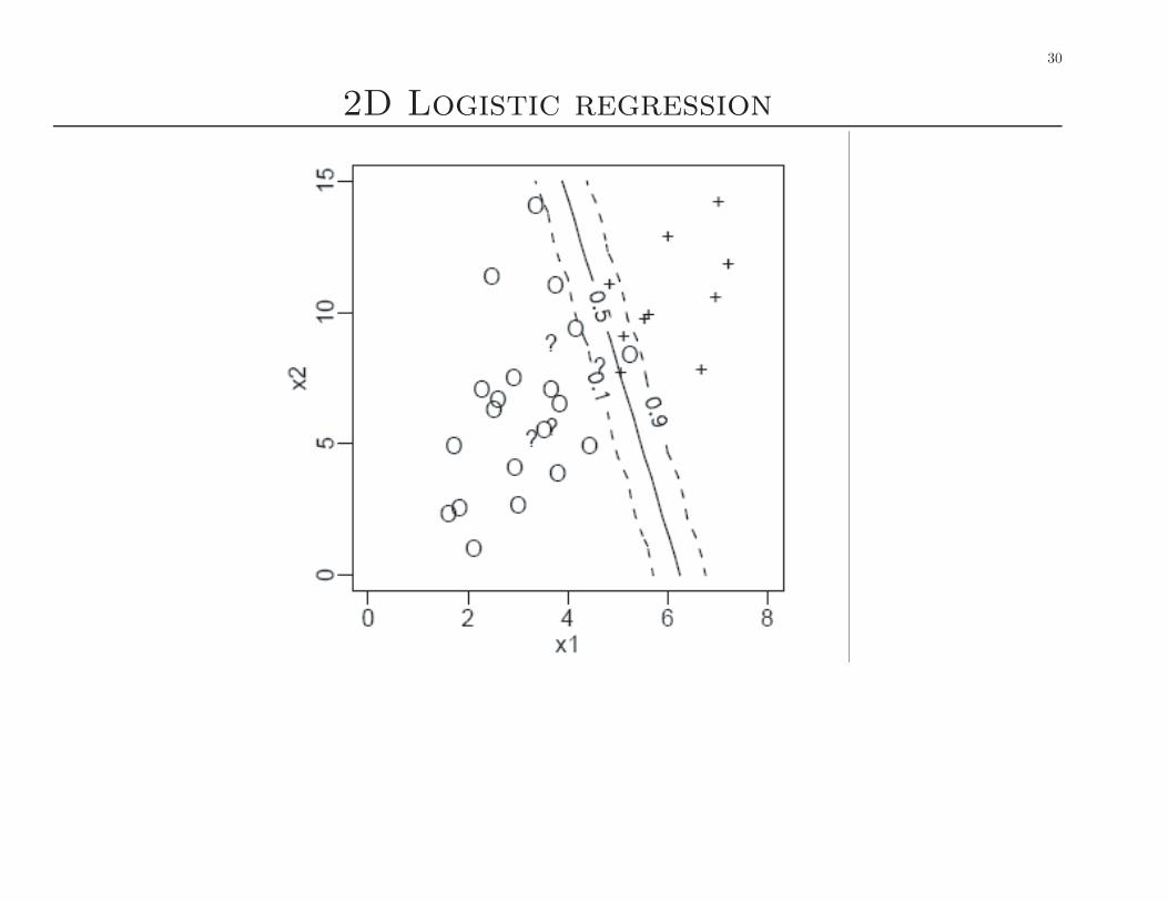
Logistic regression

• A simple approach to binary classification is logistic regression (brieflystudied in 306).

• The output density is Bernoulli conditional on x:

p(y|x) = π(x)y (1 − π(x))1−y

where y ∈ {0, 1} and

π(x) = σ(~wT [1, x1, x2])

where

σ(u) =1

1 + e−u

is the sigmoid (logistic) function that maps IR to [0, 1]. Hence

P (Y = 1|~x) =1

1 + e−w0+w1x1+w2x2

where w0 is the bias (offset) term corresponding to the dummy col-umn of 1s added to the design matrix.

30

2D Logistic regression

31

Non-linearly separable 2D data

In 306, this is called “checkerboard” data.In machine learning, this is called the “xor” problem.The “true” function is y = x1 ⊕ x2.The decision boundary is non-linear.

32

Logistic regression with quadratic features

We can separate the classes using

P (Y = 1|x1, x2) = σ(wT [1, x1, x2, x21, x

22, x1, x2])

33

Outline




• Real-world applications of regression.√

• Simple examples of classification.√


34

Handwritten digit recognition

Multi-class classification.

35

Gene microarray expression data

Rows = examples, columns = features (genes).Short, fat data (p � n).Might need to perform feature selection.

36

Other examples of classification

• Email spam filtering (spam vs not spam)

•Detecting credit card fraud (fraudulent or legitimate)

• Face detection in images (face or background)

•Web page classification (sports vs politics vs entertainment etc)

• Steering an autonomous car across the US (turn left, right, or gostraight)

stat 406: algorithms for classification and prediction lecture...

Documents