starlab technical note for samosa wp4 - satoc technical note for samosa wp4 5 1.deramp 2.2d data...

STARLAB Technical Note for SAMOSA WP4 1

Theoretical Model for SAR altimeter mode processed echoes over ocean sur-faces - Revised

Authors: C. Martin-PuigCo-Authors: G. Ruffini, J. MarquezDelivery Date: 30th September 2008Project: SAMOSA Status: Distributed to ESA and SATOC

Abstract

This Technical Note (TN) derives a theoretical model for Synthetic Aperture Radar (SAR) altimeter(also known as a as delay/Doppler radar altimeter) echoes over ocean surfaces, in the same spirit setby conventional altimeters(Brown, G.S., 1977) (Hayne, G.S., 1980). This work is done under WP4 SARAltimeter echo over water of the SAMOSA project (ESA funded). The model is needed for the effi-cient/optimal retracking of the individual delay - Doppler (DD) waveforms (task to be done in WP5)

Here we will discuss:

1. SAR Altimeter phase history

2. Deramp

3. Along track Fourier transform (AFFT)

4. Doppler Frequency

5. Earth Curvature

6. Range Cell Migration (RCM)

7. Inverse Fourier Transform (IFFT)

8. SAR Altimeter complex waveform

9. Scattered field

10. System point target response

11. surface elevation probability density

12. average flat surface impulse response


Contents

1 Notation and Definitions 31.1 Acronyms . . . . . . . . . . . . . . . . . . . . . . . . . . . . . . . . . . . . . . . . . . . . . 31.2 Cartesian system . . . . . . . . . . . . . . . . . . . . . . . . . . . . . . . . . . . . . . . . . 31.3 Fast time and Slow time . . . . . . . . . . . . . . . . . . . . . . . . . . . . . . . . . . . . . 31.4 Expectation . . . . . . . . . . . . . . . . . . . . . . . . . . . . . . . . . . . . . . . . . . . . 3

2 SAR Altimeter Phase History of a Scatterer 32.1 Deramp . . . . . . . . . . . . . . . . . . . . . . . . . . . . . . . . . . . . . . . . . . . . . . 52.2 2D Storage . . . . . . . . . . . . . . . . . . . . . . . . . . . . . . . . . . . . . . . . . . . . 62.3 Along Track FFT . . . . . . . . . . . . . . . . . . . . . . . . . . . . . . . . . . . . . . . . . 6

2.3.1 Doppler Frequency . . . . . . . . . . . . . . . . . . . . . . . . . . . . . . . . . . . . 72.3.2 Earth Curvature . . . . . . . . . . . . . . . . . . . . . . . . . . . . . . . . . . . . . 72.3.3 AFFT Output . . . . . . . . . . . . . . . . . . . . . . . . . . . . . . . . . . . . . . 8

2.4 Range Cell Migration (RCM) . . . . . . . . . . . . . . . . . . . . . . . . . . . . . . . . . . 82.4.1 Delay phase coefficient . . . . . . . . . . . . . . . . . . . . . . . . . . . . . . . . . . 82.4.2 Output of RCM block . . . . . . . . . . . . . . . . . . . . . . . . . . . . . . . . . . 8

2.5 Inverse Fourier Transform (IFFT) . . . . . . . . . . . . . . . . . . . . . . . . . . . . . . . 82.6 SAR Altimeter Mean Return Waveform . . . . . . . . . . . . . . . . . . . . . . . . . . . . 9

3 Scattered field by the ocean surface 93.1 Accumulation . . . . . . . . . . . . . . . . . . . . . . . . . . . . . . . . . . . . . . . . . . . 103.2 Plane Wave Propagation z dependence . . . . . . . . . . . . . . . . . . . . . . . . . . . . . 113.3 Complex Waveform After IFFT z Dependence . . . . . . . . . . . . . . . . . . . . . . . . . 123.4 Mean Intensity Received Previous to Multi-look . . . . . . . . . . . . . . . . . . . . . . . . 143.5 Mean Intensity After Incoherent Integration . . . . . . . . . . . . . . . . . . . . . . . . . . 153.6 Meric Srokosz’s Comments . . . . . . . . . . . . . . . . . . . . . . . . . . . . . . . . . . . . 163.7 Peter Challenor’s Comments . . . . . . . . . . . . . . . . . . . . . . . . . . . . . . . . . . . 173.8 ESA Detailed review . . . . . . . . . . . . . . . . . . . . . . . . . . . . . . . . . . . . . . . 193.9 General Review and Conclusions response . . . . . . . . . . . . . . . . . . . . . . . . . . . 20


1 Notation and Definitions

1.1 Acronyms

TN Technical noteSAR Synthetic Aperture RadarESA European Space AgencyDD Delay Doppler

AFFT Along track Fourier TransformRCM Range Cell MigrationIFFT Inverse Fourier TransformPRF Pulse Repetition FrequencyDDA Delay Doppler Altimeter

FT Fourier TransformRCS Radar Cross Section

pdf Probability density function

1.2 Cartesian system

As cartesian system in what follows we will use axis defined by (x,y,z). Here x defines the along trackdirection, y the across track direction and z axis directed upward. An arbitrary point N in our geometrywill be specified by (xn,yn,z). The variable z corresponds to the surface elevation, also referenced in someliterature as z = h(r) = h(x, y), a realization of a random stationary process.

1.3 Fast time and Slow time

In section 2.2 one of the SAR altimeter processing blocks (2D Storage) is briefly described. In thisblock the received data is stored in a two dimensional matrix prior to Doppler processing. This matrixhas as rows the samples of the waveforms (aka Delay/continuous wave), and as columns the differentwaveforms received (also known as the line number). According to CryoSat’s specifications (ESA, 2007)the matrix dimensions should be 256 rows (128 complex samples per waveform), and 64 columns (oneecho per emitted pulse). Therefore, there will be one matrix per burst. In some SAR literature the rowsare represented by the variable t′ or fast time, and the columns are represented by the variable t or slowtime. Although both variables represent time, different processing steps are applied to each of them.From this point forward, t or slow time, and t′ or fast time will be used to refer to the matrix axis.

1.4 Expectation

Let X be a continuous random variable (r.v.) with probability density function (pdf) fX(x), let g(x) bea function of x; the expected value of g(x) is defined as:

E[g(x)] =∫ ∞−∞

g(x)fX(x)dx (1.1)

2 SAR Altimeter Phase History of a Scatterer

This section aims to analyze the phase history of a single scatterer for a SAR Altimeter (Raney, R.K.,1998). This analysis is after used to derive the mean return echo waveform over ocean surfaces of suchaltimeter (see section 3).


The CryoSat altimeter operating in SAR mode emits 64 coherent pulses per burst at a pulse repeti-tion frequency (PRF) of 17.8 kHz (ESA, 2007) with a burst repetition frequency of 85.7 Hz. The emittedpulses are modulated as chirps with a BW = 350 MHz and a transmitted pulse length τp = 49µs.

For the phase history of a single scatterer N at arbitrary position N = (xn, yn, z) (see Figure 1) wewill consider that a chirp pulse C(t′) is transmitted from the sensor, reflects on the scatterer and returnsback traveling twice the distance r(t). Therefore, the two-way return chirp of a single scatterer N will bedelayed by: C(t′− 2r(t)

c ); being c equal to the speed of light (c = 3·108m/s), r2(t) = ∆x(t)2+y2n+(H−z)2,

H = 717.242Km the CryoSat mean altitude, and ∆x(t) the distance between the satellite position andxn the along track position of the nth scatterer (Raney, R.K., 1998).

The spacecraft propagates in along-track (x, t) with velocity Vs. Therefore, the two-way traveled distancer(t) also varies with t (slow time), and so does ∆x(t) = (x0 − xn) − Vst. Note that ∆x(t) is referencedto x0, which corresponds to a reference satellite nadir position within a burst (e.g. the satellite nadirposition at the beginning of the burst).

Figure 1: Observation scene

r2(t) = ∆x(t)2 + y2n + (H − z)2

r(t) ≈ H +(∆x(t)2 + y2

n − 2Hz + z2)2H

(2.1)

The SAR Altimeter concept is described in depth in (Raney, R.K., 1998); the main processing steps, ifno vertical spacecraft component is considered1, are:

1If the spacecraft’s vertical velocity component is considered, an additional block previous to AFFT shall be added to


1. deramp

2. 2D data storage

3. Along track FFT (AFFT)

4. Delay Phase Coefficients

5. Delay Inverse FFT (IFFT)

6. Accumulation

7. Multi - Look (also known as as look integration)

This technical note does not provide a detailed description of each block. However, the input and outputdata of the first five blocks, as well as a brief description is detailed in the fortcoming subsections. Thelast two blocks will be addressed in Section 3.

2.1 Deramp

The first processing step in a DD Altimeter (DDA) is the deramp (Chelton et al, 1989). This techniquetransforms the received echo in a continuous wave (CW) whose frequency is linearly related to the traveltime, and hence the radar range of each individual backscattering element relative to the 4t = td− 2r(t)

c(td is known as the deramp time delay).

Considering a transmitted chirp signal C(t′) = ei2π(f0+ s2 t′)t′ with 0 ≤ t′ ≤ τp, where s is the chirp

slope s = BWτp

; the received backscattered echo C(t′− 2r(t)c ) 0 ≤ t′ ≤ τp is multiplied by a deramp replica

Cd(t′ − td) = C∗(t′ − td) 0 ≤ t′ ≤ τp resulting into:

w(t′, t) = ei∆φ(t′,t) (2.2)

∆φ(t′, t) = w0(td −2r(t)c

) + 2πs(td −2r(t)c

)t′ + πs((2r(t)c

)2 − t2d) (2.3)

If r(t) is replaced by Eq. 2.1 and td is considered to be well adjusted td = t0, and t0 = 2Hc , and Ks = sπ

∆φ(t′, t) = −w0

cH∆x(t)2 − w0

cH(y2n − 2Hz + z2)− 2ks

cH(∆x(t)2 + y2

n − 2Hz + z2)(t′ − t0) (2.4)

The first term, with a quadratic dependence on the satellite position will mostly contribute in the alongtrack processing enhancing the along-track resolution. The second term is a constant for the DDAprocessing. Finally, the third term will define the RCM correction. Range Migration is an effect visualafter along track FFT caused by time variability of range to target; the effect is that the compressedpoint target response occurs at different range gates for different pulses (Curlander et al., 1991).

compensate for this component effect. The final complex waveform after the IFFT block will be the same independently ofthis additional component. For mathematical simplicity it will not be considered in this TN, thus we have ~Vs = (Vsx, 0, 0).


2.2 2D Storage

The second processing block is the 2D data storage. As introduced in 1.3, in the form of a matrix allthe echoes received within one burst are stored. This process is equivalent to applying an along trackfilter of length T , hereafter referred as coherence time, and also an across track filter of length the pulseuseful length τu. Therefore, we can express the outcome of this block as2 :

W (t′, t) = w(t′, t)∏

(t′

τu)∏

(t

T) (2.5)

2.3 Along Track FFT

The third block is the along track Fourier Transform (AFFT), which only affects the along track termsof W (t′, t). The non along track dependent terms are defined is this section as Wr(t′):

W (t′, t) = Wr(t′) e−i(w0cH+ 2ks

cH (t′−t0))∆x(t)2∏

(t

T) (2.6)

where Wr(t′):

Wr(t′) = e−i(y2n−2Hz+z2)

cH (w0+2ks(t′−t0))

∏(t′

τu) (2.7)

The AFFT is defined as:

Wa(t′, fa) = Wr(t′)∫ ∞−∞

e−i(w0cH+ 2ks

cH (t′−t0))∆x(t)2∏

(t

T) e−i2πfatdt (2.8)

Where fa refers to the along track frequency domain.

Before further proceeding with the analysis the multiplying term w0cH + 2ks

cH (t′ − t0) is evaluated. Onone hand, after the 2D storage the fast time t′ is limited to τu. On the other hand, we have previouslydefined t0 = 2H

c . By numerical comparison for the CryoSat specifications (ESA, 2007) the term fasttime dependent (term multiplying t′) is smaller than the other terms (w0, t0 dependent), thus it can beneglected during integration.

Wa(t′, fa) = Wr(t′) e−i2KscH t′∆x(t)2

∫ ∞−∞

e−i(w0−2Ksto)

cH ∆x(t)2∏

(t

T) e−i2πfatdt (2.9)

If we substitute ∆x(t) = (x0 − xn)− Vst

Wa(t′, fa) 'Wr(t′) e−i2KscH t′∆x(t)2

∫ ∞−∞

e−i(w0−2Ksto)

cH ((x0−xn)2−2(xo−xn)Vst+(Vst)2)

∏(t

T) e−i2πfatdt

(2.10)Eq. 2.10 shows a quadratic dependence of the exponent with the variable t (slow time). If this quadraticterm was not present the integral would simplify to the FT of a pulse signal, which is known to be a sincfunction. The quadratic term defines a chirp signal in azimuth. Echoes received within a small ∆t fromthe origin of this chirp will add in phase, whereas those from farther out in t will cancel out. The maineffect is that those t close to the origin [−∆t,∆t] integrate to a non zero value, whereas those fartheraway integrate to zero. This integration ”condition” effectively selects only the portion of the returnsnear the origin of the chirp azimuth signal, improving the resolution by rejecting energy from larger tvalues (larger doppler frequencies). This ”condition” is known as Unfocused SAR.

2The function∏

(t) defines a uniform distribution


Furthermore, the resolution achieved with unfocused SAR processing can be quantified by knowing whatarea on the ground corresponds to the central region of azimuth return that contributes to the output ofthe integrator. Assuming that only signals with a phase deviation of less than π/4 over the integrationinterval contribute meaningfully to the point response, the distance on the ground corresponding to thisphase difference can be calculated. The choice of π/4 phase difference is a little arbitrary an other optionsare occasionally used (e.g. π/8). The basis of this choice is the stationary phase approximation.

∆φa(t) = |φa(T

2)− φa(0)| ≤ π

4

| (w0 − 2Ksto)cH

V 2s (T

2)2| ≤ π

4

V 2s T

2 ≤ Hλ0

21

|1− 2HBWτpcf0

|

‖VsT‖ = ‖δa‖ ≥√

0.66λ0H

2(2.11)

The previous equation provides an along track resolution almost equal to the dimensions of the firstFresnel zone. In addition, it also shows a limit on T, since Vs is assumed constant. If T is set to satisfythis condition, the quadratic term in Eq. 2.10 satisfies stationary phase and the overall AFFT can besimplified to:

Wa(t′, fa) = Wr(t′)e−i2KscH t′∆x(t)2

∫ T2

−T2e−i

(w0−2Ksto)cH ((x0−xn)2−2(xo−xn)Vst) e−i2πfatdt (2.12)

Before further proceeding with the AFFT it is convenient to analyse at this point two parameters relatedto our observation which have not been introduced previously: Doppler frequency and Earth Curvature.

2.3.1 Doppler Frequency

The along track movement of the spacecraft will introduce a doppler frequency to the observation. Ac-cording to (Raney, R.K., 1998) the Doppler frequency is given by:

fD =2λo

~r(t− tn) · ~Vs‖~r(t− tn)‖

(2.13)

”within the constrain of the near-vertical small angle geometry of a satellite altimeter, the Doppler scalingfactor is approximated very well by” (Raney, R.K., 1998):

fD ≈2Vsλo

(x0 − xn)H

(2.14)

2.3.2 Earth Curvature

It can be shown that for curve surfaces the distance from the satellite sensor to the scatterer is related tor(t) (previously described) as: r′(t) = r(t) + δrx(t). If this is deeply analyzed we can demonstrate that:

r′(t) = H +(α∆x(t)2 + y2

n − 2Hz + z2)2H

(2.15)

With α = 1 + HRE

, where RE is the Earth radius. It is clear from 2.15 that to account for curvatureeffects an α∆x2(t) factor shall be substituted in all the previous equations instead of ∆x2(t).


2.3.3 AFFT Output

Results in sections 2.3.1 and 2.3.2 are this point forward introduced in our analysis. Therefore, Eq.2.12 may be written as:

Wa(t′, fa) = T Wr(t′) e−i2KscH α∆x(t)2t′e

−iαπf2

DHc

2f0V2s

(1− stof0 )sinc (

T

2π(wa − αwD(1− st0

f0))) (2.16)

2.4 Range Cell Migration (RCM)

RCM was already introduced in section 2.1. The RCM block in the SAR altimeter is based on themultiplication of a Delay phase coefficient, which compensates for the range curvature effect (Raney,R.K., 1998). The waveform input to this block equals to:

Wa(t′, fa) = Te−i(y2n−2Hz+z2)

cH (w0+2ks(t′−t0)) e−i

2KscH α∆x(t)2t′ e

−iαπf2

DHc

2f0V2s

(1− stof0 )

sinc (T


f0)))

∏(t′

τu) (2.17)

2.4.1 Delay phase coefficient

Analyzing the previous equation it can be shown that the curvature effect will be introduced by theterm 2ks

cH α∆x2t′. Therefore, the delay phase coefficient multiplying the waveform after the azimuth FFTaccounting for Earth curvature should be:

φ(t′, t) = ei2kscH α∆x(t)2t′ (2.18)

Which expressed as a function of the doppler frequency is equal to:

φ(t′, t) ≈ ei2πs2cα

αf2Dλ20H

8Vst′ (2.19)

2.4.2 Output of RCM block

The multiplication of the phase delay achieved in the previous subsection with our waveform at theoutput of the AFFT block results into:

Wa(t′, fa) = Te−i(y2n−2Hz+z2)

cH (w0+2ks(t′−t0)) e

−iαπf2

DHc

2f0V2s

(1− stof0 )sinc (

T


f0)))

∏(t′

τu)

(2.20)

2.5 Inverse Fourier Transform (IFFT)

The final block previous to accumulation and incoherent averaging is the IFFT in fast time (t′) of theRCM corrected signal. Since this transform only affects the contributions in fast time, the non fast timeterms will be referred in this section as Wa(fa).

WRCM (t′, fa) = Wa(fa) e−i2kscH (y2

n−2Hz+z2)(t′−t0)∏

(t′

τu) (2.21)


being,

Wa(fa) = T e−iw0cH (y2

n−2Hz+z2) e−i

απf2DHc

2f0V2s

(1− stof0 )sinc (

T


f0))) (2.22)

The IFFT is defined as:

W (τ, fa) =∫ ∞−∞

WRCM (t′, fa) ei2πt′τdt′

= Wa(fa) ei2kscH (y2

n−2Hz+z2)t0

∫ ∞−∞

e−i2kscH (y2

n−2Hz+z2)t′∏

(t′

τu) ei2πt

′τdt′ (2.23)

Like in section 2.1 we are now left with the FT of a normal distributed signal with a frequency dependenceon fast time parameters.

W (τ, fa) = Wa(fa) ei2kscH (y2

n−2Hz+z2)t0

∫ τu2

− τu2e−i2π( s

cH (y2n−2Hz+z2)−τ)t′dt′

= τu Wa(fa) ei2kscH (y2

n−2Hz+z2)t0 sinc (τu(s

cH(y2n − 2Hz + z2)− τ)) (2.24)

2.6 SAR Altimeter Mean Return Waveform

The final complex waveform before accumulation will be equal to:

W (τ, fa) = T τu e−i (y

2n−2Hz+z2)

cH (w0−2kst0) e−i

απf2DHc

2f0V2s

(1− stof0 )

sinc(T


f0))) sinc (τu(

s

cH(y2n − 2Hz + z2)− τ)) (2.25)

3 Scattered field by the ocean surface

Knowing the phase history of a single scatter, the second step of the definition of a SAR altimeter meanreturn waveform is to detail the scattered field received at the sensor not only by a single scatter, but by asum of scatters within the illuminated area. Precisely, it is important to analyze which is the dependenceof the backscattered field with the surface under observation. For this reason, our starting point will bebased on the asymptotic expression of the field scattered by the ocean surface when illuminated by aquasi - monochromatic spherical wave and in a frozen geometry (emitter, receiver and surface are staticduring integration time). Following (Beckman et al., 1963) and (Born et al., 1999), and considering thegeometry in Figure 2 the scattered field at far distances can be written as a coherent sum of elementarycontributions of each point on the illuminated surface.

E(k, t′) =1Lp

∫surf

√G(~ρ) S(~ρ) C(t′ − ‖ ~rT ‖

c)

√Aeff

eik(‖~r‖+‖~r′‖−ct′)

‖~r‖‖~r′‖d2~ρ (3.1)

Being Lp the total propagation loss, G(~ρ) the transmitting antena gain, S(~ρ) the surface scatteringamplitude (e.g. obliquity function), rT the total distance traveled ~rT = ~r− ~r′, ‖~r‖ the distance from thetransmitter to the scattering point, ‖~r′‖ the distance from the scattering point to the receiving antenna,c the speed of light, Aeff the area effective of the receiving antenna and k the wavenumber k = 2π

λ0. If

the effective area in power is related to the gain as: Aeff = Gλ20

4π then:


Figure 2: Observation Scene Geometry

E(k, t′) =λ0√4πLp

∫surf(~ρ)

G(~ρ) S(~ρ) C(t′ − ‖~r −~r′‖

c)eik(‖~r‖+‖~r′‖−ct′)

‖~r‖‖~r′‖d2~ρ (3.2)

From Figure 2 it is easy to relate ~r′ = −~r. Therefore, the previous equation further simplifies to:

E(k, t′) =λ0√4πLp

∫surf(~ρ)

G(~ρ) S(~ρ) C(t′ − 2‖~r‖c

)eik(2‖~r‖−ct′)

‖~r‖2d2~ρ (3.3)

The received backscatter electric field will be input to the SAR processing chain. If we consider noantenna dependence on slow time, nor surface scattering amplitude dependence; the complex waveformat the output of the SAR altimeter if we introduce this backscatter field will be:

Es(τ, fa; z) =λ0√4πLp

∫surf(~ρ)

G(~ρ) S(~ρ) W (τ, fa; ~ρ, z)eik(2‖~r‖)

‖~r‖2d2~ρ (3.4)

Being τ the delay time, fa the azimuth frequency domain, and z the surface altitude at ~ρ. This pointforward we will express z either as z or z(~ρ), the same for z(~ρ′) = z′. W (τ, fa) full expression shall befound in section 2.6. The only change here with respect Eq. 2.25 is that it has been made clear thedependence of the complex waveform with ~ρ and z.

3.1 Accumulation

After the IFFT block the different waveforms within the burst are ‖ ‖2 transformed. The accumulationprocess provides us the received intensity, which may be defined as:

IR = Es(τ, fa; z(~ρ)) E∗s (τ, fa; z(~ρ′)) (3.5)


Our interest in this section is focus on the mean intensity after accumulation and previous to multi-look.The result achieved in this section is after analyzed to account for multi-look of the SAR altimeter.

E[IR]z = E[Es(τ, fa; z(~ρ)) E∗s (τ, fa; z(~ρ′))]z (3.6)

If Eq. 3.4 is substituted in the previous expression,

E[IR]z = E[λ2

0

4πL2p

∫~ρ

∫~ρ′G(~ρ) G∗(~ρ′) S(~ρ) S∗(~ρ′) W (τ, fa; z) W ∗(τ, fa; z′)

ei2k(‖~r‖−‖~r′‖)

‖~r‖2‖~r′‖2d2~ρ d2~ρ′]z (3.7)

Where r = r(z, ~ρ). If the mean is done over z we can well approximate the previous as:

E[IR]z =λ2

0

4πL2p

∫~ρ

∫~ρ′G(~ρ) G∗(~ρ′) S(~ρ) S∗(~ρ′) E[W (τ, fa; z) W ∗(τ, fa; z′)

ei2k(‖~r‖−‖~r′‖)

‖~r‖2‖~r′‖2]z d2~ρd2~ρ′ (3.8)

With the aim to simplify the previous expression let the next sections focus on the independent analysisof the different terms inside the expectation.

3.2 Plane Wave Propagation z dependence

In this section we will analyze the z dependence of:

ei2k(‖~r(z,~ρ)‖−‖~r(z′,~ρ′)‖)

‖~r(z, ~ρ)‖2‖~r(z′, ~ρ′)‖2(3.9)

According to Figure 2 ~r = ~r0 + ~ξ(z). Being ~r0 = roρρ − roz z, and ~ξ(z) = zz. Doing such substitution

the ‖~r‖ =√r2oρ + (z − r0z)2 =

√r2oρ + r2

0z − 2zr0z + z2 =√‖~r0‖2 − 2zr0z + z2. Note r0z = H. Since

z � H the term z2 can be neglected and the expression of ‖~r‖ can be approximated by Taylor series to:

‖~r‖ = ‖~r0‖ −zH

‖~r0‖(3.10)

If we express this term as a function of the inclination angle ε, being sin(ε) = H‖~r0‖ . The previous can be

expressed as:

‖~r‖ = ‖~r0‖ − z sin(ε) (3.11)

We are also interested in analyzing the dependence of this phase term with ρ, thus we can expressr2o = ‖~ro‖2 = ‖~ρ‖2 +H2. ‖~ρ‖ can be approximated as: ‖~ρ‖ = ρ0 + δ~ρ, and using Taylor series we finally

achieve:

‖~r0‖ ≈ H +ρ2

0

2H+ρ0δ~ρ

H(3.12)

Consequently,

‖~r‖ ' H +ρ2

0

2H+ρ0δ~ρ

H− z sin(ε) (3.13)

Considering the previous analysis where H, ρ0, and ε are invariable, and doing the approximation in thedenominator of ‖~r‖2 = ‖~r′‖2 = H2; Eq. 3.9 is equal to:

ei2k(ρ0H (δ~ρ−δ~ρ′)−sin(ε)(z−z′))

H4=ei2k(

ρ0H ∆ρ−sin(ε)(z−z′))

H4(3.14)

where ∆ρ = δ~ρ− δ~ρ′.


3.3 Complex Waveform After IFFT z Dependence

The complex waveform achieved after the IFFT block of the SAR altimeter (Eq. 2.25) shall be written foranalysis simplification as a function of: all the terms z dependent, and a multiplying function W0(fa; ~ρ)which will account for all the non z dependent terms.

W (τ, fa; ~ρ) = W0(fa; ~ρ) e−i(−2Hz+z2)(w0−2kst0)

cH sinc (τu(s

cH(y2n − 2Hz + z2)− τ)) (3.15)

Where

W0(fa; ~ρ) = T τu e−i y

2n(w0−2kst0)

cH e−i

απf2DHc

2f0V2s

(1− stof0 )sinc (

T


f0))) (3.16)

Note that yn and fD are functions of ~ρ, since ‖~ρ‖2 = x2n + y2

n, and fD is a function of xn.

Let us analyze the different terms in the z exponential dependence of the function W (τ, fa; ~ρ) (Eq.2.25). A quadratic z dependence and a linera z dependence are present in the exponential term. IfCryoSat specifications are substituted (ESA, 2007), and knowing that z � H, it can be proved that thequadratic term contribution is smaller than the liner one. Therefore, this point forward we will neglectits contribution, and express Eq. 2.25 as:

W (τ, fa; ~ρ) 'W0(fa; ~ρ) ei2(w0−2kst0)z

c sinc (τu(s

cH(y2n − 2Hz + z2)− τ))3 (3.17)

Going back to Eq. 3.8 where the function W (τ, fD; ~ρ) is multiplied by W ∗(τ, fD; ~ρ), thus:

W (τ, fa; ~ρ)W ∗(τ, fa; ~ρ′) = W0(fa; ~ρ) W ∗0 (fa, ~ρ′) ei2(w0−2kst0)(z−z′)

c

sinc (τu(s

cH(y2n − 2zH)− τ)) sinc (τu(

s

cH(y′2n − 2z′H)− τ)) (3.18)

Analyzing the expectation,

E[W (τ, fa; ~ρ) W ∗(τ, fa; ~ρ)ei2k(‖~r‖−‖~r′‖)

‖~r‖2‖~r′‖2]z = E[W0(fa; ~ρ) W ∗0 (fa, ~ρ′) ei

2(w0−2kst0)(z−z′)c

sinc (τu(s


s

cH(y′2n − 2z′H)− τ))

ei2k(ρ0H ∆ρ−sin(ε)(z−z′))

H4]z (3.19)

Some of the previous equation terms are not z dependent, and can be moved out of the expectationmeasurement:

E[W (τ, fa; ~ρ) W ∗(τ, fa; ~ρ)ei2k(‖~r‖−‖~r′‖)

‖~r‖2‖~r′‖2]z = W0(fa; ~ρ) W ∗0 (fa, ~ρ′)

ei2kρ0H ∆ρ

H4E[ ei

2(w0−2kst0)(z−z′)c

sinc (τu(s


s

cH(y′2n − 2z′H)− τ))

e−i2k sin(ε)(z−z′)]z (3.20)3remember the dependence of yn with ρ


Let U = z − z′ be a new r.v. . If U is independent of z, and z′, the expectation value will result into amultiplication of expectations. For this to happen, z and z′ must be really close to each other, thus verycorrelated. If we assume Gaussian statistics for z and z′, both zero mean, and define z′ = z − δz, and δzindependent of Z, Gaussian r.v. with zero mean and standard deviation σδz very small:

E[Uz] = E[(z − z′)z] = E[δzz] = 0 (3.21)

if δz and z are independent the previous equation results into a multiplication of means which equal to0. Therefore, we can say that U and z are uncorrelated, and provided they are Gaussian signals withzero mean both of them, it can be proved that they are also independent. This approximation leads usto express Eq. 3.20 as the product of two expectations:

E[W (τ, fa; z) W ∗(τ, fa; z′)ei2k(‖~r‖−‖~r′‖)

‖~r‖2‖~r′‖2]z =

W0(fa) W ∗0 (fa) e−i(w0−2kst0)

cH (y2n−y

′2n ) e

i2kρ0H (δ~ρ−δ~ρ′)

H4E[e−i2(

−(w0−2kst0)c +k sin(ε))(z−z′)]

E[sinc (τu(s

cH(y2n − 2zH)− τ))sinc (τu(

s

cH(y′2n − 2z′H)− τ))]z (3.22)

The first expectation value can be proved to be equal to the next expression assuming Gaussian statisticsfor the ocean (∆ρ small) (Beckman et al., 1963):

E[e−i2(−(w0−2kst0)

c +k sin(ε))(z−z′)]z = e−4(−(w0−2kst0)

c +k sin(ε))2σ2z [1−C(4~ρ)] (3.23)

where σz is the standard deviation of the surface elevation, and C(4~ρ) the spatial autocorrelation functionof the sea surface. Previously we have considered points near the origin (∆ρ ' 0), for such scene thespatial autocorrelation can be approximated by a Gaussian function (Beckman et al., 1963):

C(4~ρ) = e−4~ρ2

2l2C ' 1− 4ρ

2

2l2c(3.24)

If we substitute Eq. 3.24 in Eq. 3.23:

E[e−i2(−(w0−2kst0)

c +k sin(ε))(z−z′)]z = e−4(

−(w0−2kst0)c +k sin(ε))2σ2

z4ρ2

2l2c (3.25)

The previous equation shows that the expectation of the exponential term results into a Normal dis-tributed function over ∆ρ with zero mean and standard deviation:

σ4ρ =lc

2σz(−(w0−2kst0)

c + ksin(ε))(3.26)

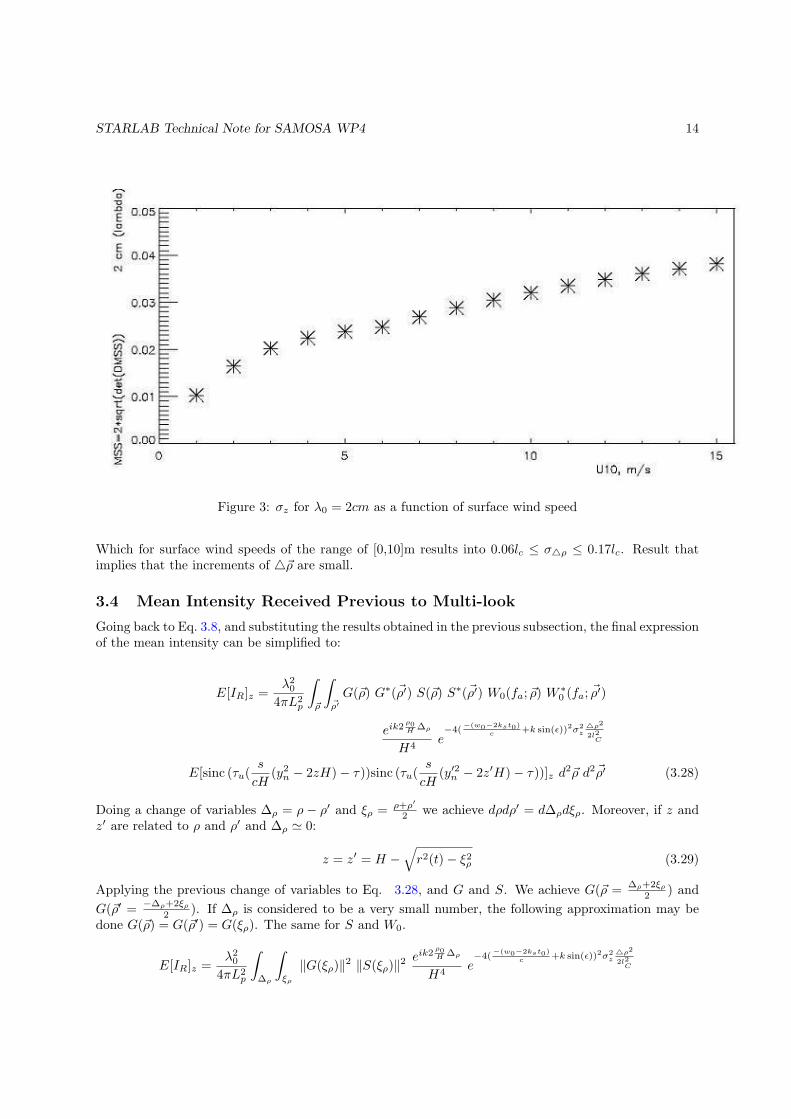
Elevation standard deviation measurements for different surface wind speeds and λ0 = 2cm have beensimulated at Starlab based on (Elfouhaily et al., 1997), the results are shown in Figure 3. The simulationwas carried for wind speeds from 1 to 25 m/s.out and a mature sea, with a resolution of 4 cm covering asquare of 300 m in each side.

For CryoSat λ0 = 2.22cm so we can approximate the values of σz by the results provided in the previousfigure. The other terms within the equation are available in different sections of this TN, evaluatingnumerically this terms it can be shown that (w0−2kst0)

c � k sin(ε), thus σ can be approximated by:

σ4ρ 'lcλ0

4πσz(3.27)


Figure 3: σz for λ0 = 2cm as a function of surface wind speed

Which for surface wind speeds of the range of [0,10]m results into 0.06lc ≤ σ4ρ ≤ 0.17lc. Result thatimplies that the increments of 4~ρ are small.

3.4 Mean Intensity Received Previous to Multi-look

Going back to Eq. 3.8, and substituting the results obtained in the previous subsection, the final expressionof the mean intensity can be simplified to:

E[IR]z =λ2

0

4πL2p

∫~ρ

∫~ρ′G(~ρ) G∗(~ρ′) S(~ρ) S∗(~ρ′) W0(fa; ~ρ) W ∗0 (fa; ~ρ′)

eik2ρ0H ∆ρ

H4e−4(


z4ρ2

2l2C

E[sinc (τu(s

cH(y2n − 2zH)− τ))sinc (τu(

s

cH(y′2n − 2z′H)− τ))]z d2~ρ d2~ρ′ (3.28)

Doing a change of variables ∆ρ = ρ − ρ′ and ξρ = ρ+ρ′

2 we achieve dρdρ′ = d∆ρdξρ. Moreover, if z andz′ are related to ρ and ρ′ and ∆ρ ' 0:

z = z′ = H −√r2(t)− ξ2

ρ (3.29)

Applying the previous change of variables to Eq. 3.28, and G and S. We achieve G(~ρ = ∆ρ+2ξρ2 ) and

G(~ρ′ = −∆ρ+2ξρ2 ). If ∆ρ is considered to be a very small number, the following approximation may be

done G(~ρ) = G(~ρ′) = G(ξρ). The same for S and W0.

E[IR]z =λ2

0

4πL2p

∫∆ρ

∫ξρ

‖G(ξρ)‖2 ‖S(ξρ)‖2eik2

ρ0H ∆ρ

H4e−4(


z4ρ2

2l2C


E[‖W0(fa; ξρ)‖‖2sinc (τu(s

cH(y2n − 2H(H −

√r2(t)− ξ2

ρ))− τ))‖2]z d2ξρ d2∆ρ (3.30)

Which is equal to:

E[IR]z =λ2

0

4πL2pH

4

∫∆ρ

∫ξρ

‖G(ξρ)‖2 ‖S(ξρ)‖2 eik2ρ0H ∆ρ e

−4(−(w0−2kst0)

c +k sin(ε))2σ2z4ρ2

2l2C E[‖W (τ, fa; ξρ)‖2]z d2ξρ d

2∆ρ

(3.31)This point forward we will refer to σo to:

σ0(ε) =∫

∆ρ

eik2ρ0H ∆ρ e

−4(−(w0−2kst0)

c +k sin(ε))2σ2z4ρ2

2l2C d2∆ρ (3.32)

Which simplifies Eq. 3.30 to:

E[IR]z =λ2

0

4πL2pH

4

∫ξρ

‖G(ξρ)‖2 ‖S(ξρ)‖2 σ0(ε) E[‖W (τ, fa; ξρ)‖2]z d2ξρ (3.33)

From the (Hayne, G.S., 1980), or from the definition of the expectation, the next equality can be done:

E[‖W (τ, fa; ξρ)‖2]z = ‖W (τ, fa; ξρ)‖2 ∗ qz(τ) = SR(τ, fa; ξρ) ∗ qz(τ) (3.34)

W (τ, fa; ξρ) corresponds to the complex waveform after IFFT, SR(τ, fa; ξρ) = ‖W (τ, fa; ξρ)‖2 is thesystem point targe response achieved previous to multi-look, and qz(τ) the surface pdf of the specularpoints which is defined as in (Hayne, G.S., 1980). If Eq. 3.34 is substituted in the mean intensityexpression we achieve:

E[IR]z =λ2

0

4πL2pH

4

∫ξρ

‖G(ξρ)‖2 ‖S(ξρ)‖2 σ0(ε) SR(τ, fa; ξρ) ∗ qz(τ) d2ξρ (3.35)

As in (Hayne, G.S., 1980) this can be considered the convolution of three terms E[IR]z = PFS(τ ; ξρ, ε) ∗SR(τ, fa; ξρ) ∗ qz(τ), where PFS(τ ; ξρ, ε) corresponds to the flat surface impulse response previous tomulti-look:

PFS(τ ; ξρ, ε) =λ2

0

4πL2pH

4

∫ξρ

‖G(ξρ)‖2 ‖S(ξρ)‖2 σ0(ε) δ(τ, fa) d2ξρ (3.36)

Finally, The only term here to be analyzed is: SR(τ, fD; ξρ)

SR(τ, fa; ξρ) = T 2 τ2u sinc 2(

T


f0))) sinc 2(τu(

s

cH(y2n − 2Hz + z2)− τ)) (3.37)

Both fD and yn already related to ρ, thus also related to ξρ.

3.5 Mean Intensity After Incoherent Integration

Previous to incoherent integration the waveforms are accumulated in a two dimensions matrix (cols -Doppler bins, rows - delay time)4.

4Clarification: Multi-look is based on the incoherently addition of all the contributions from the same region of theocean (region defined by the doppler bin - delay) observed by various burst during illumination time. In this section wewill account for incoherent summation of those doppler bins, thus we will apply multi-look.


After incoherent averaging the mean intensity for those Doppler bins corresponding to the same regionover the ocean the resulting waveform will be equal to:

E[IR]z =λ2

0

4πL2pH

4

M∑m=1

∫~ξρ

‖G(~ξρ− ~Vstm)‖2 ‖S(~ξρ− ~Vstm)‖2 σ0(ε− ε′) E[‖W (τm, fm; ~ξρ− ~Vstm)‖2]z d2 ~ξρ

(3.38)Where M refers to the total number of looks during illumination time, Vstm accounts for the displacementwith respect satellite nadir of the Doppler bin from one burst to another, ε′ account for the change of theinclination angle from one burst to the other, τm accounts for the time delay difference of the contributionsof the same Doppler bin in different observation geometries at each burst, and fm = fa + ∆fD accountsfor the Doppler displacement of the same bin seen from burst to burst. Considering gain, scatteringamplitude and RCS constant for all m the maximum mean intensity received would be equal to:

E[IR]z = M(PFS(τ ; ξρ, ε) ∗ SR(τ, fa; ξρ) ∗ qz(τ)) (3.39)

The total number of looks of each Doppler bin can be measured dividing the total illumination time,by the burst integration time (previously cited as coherence time T), thus: M = Ti

T = LAδa

. WhereLA stands for equivalent along track orbit integration length (Raney, R.K., 1998) defined as αβH, and

‖δa‖ ≥√

0.8λ0H2 . with this definitions M equals to:

M = β

√2Hαλ

(3.40)

Note that if (Brown, G.S., 1977) flat surface impulse response solution is used, the mean intensity will havea H−3 dependence. After incoherent addition of the different bins that span the width of the antenna,the mean intensity will be dependent on H−5/2, which resembles the solution provided in (Raney, R.K.,1998).

ANNEX 1: NOCS review

3.6 Meric Srokosz’s Comments

Having read through the revised version of the TN (technical note) I am clearer on some of the mathemat-ical assumptions and details, but not all. Lack of time precludes me checking all the mathematics. Theexplanations are better than in the first versions but there are still places where a little extra explanationwould help.

1. Equation (2.1) looks wrong. Should the second part be r(t) H+ etc?

• This equation is correct, and the proof is provide hereafter:

r2(t) = H2 + ∆x(t)2 + y2n − 2Hz + z2 = H2(1 +

x(t)2 + y2n − 2Hz + z2

H2) (3.41)

r(t) ∼ H(1 +x(t)2 + y2

n − 2Hz + z2

2H)

the approximation is achieved by applying Taylor series, and the only missing step to becoincident with Eq. 2.1 is the multiplication of H by each term within the sum.


2. Equation (2.5) is confusing as the footnote 2 looks like a power 2.

• We agree that the footnote indicator in the previous version of 2.5 may led to confusion andresemble to a power of 2. This has been changed in this final version.

3. Page 6 a reference for the stationary phase approximation would be helpful

• A good reference is ”Mathematical Methods for Physicist” of Arfken and Weber, but thestationary phase is a known method and we do not consider it necessary to be referenced inthe TN.

4. Throughout origine should be origin

• Changed

5. The final expression for E[IR]z equation (3.38) on page 15 needs to be an analytic expressionif it is to be used in fitting to the actual DDA return (see proposal). This means that analyticexpressions for PFS and SR are required as intermediate steps. SR is given in equation (3.36), butno analytic expression is given for PFS (see equation 3.35). PFS depends on G the transmittingantenna gain and S the surface scattering amplitude (obliquity function). These are introduced onpage 9, equation (3.1) but no expressions are given for their functional form. Do we know whatthey are? If so, this information should be included in the TN explicitly

• No analytical expression or closed form is provided since the retracker will be numericallyimplemented. However, in response to the last part of the comment we may add that G, andS let us add that this expressions will be identical to Brown’s as specified in the TN, thus wedid not include them in the TN.

Looking forward to the next steps in SAMOSA fitting the model presented here to data I foresee a potentialproblem. The convolution is a double integral and if that has to be evaluated numerically the fitting of thetheoretical to the actual DDA return will be computationally costly. It will also be a significantly morechallenging programming problem. The convolution (equation 3.38) is essentially in the same form asthat in Brown (1977) for a standard pulse-limited altimeter, but the details of the terms in the convolutiondiffer. Therefore, it would be helpful to have plots of some of the functions, in particular of SR and PFS,to see how they differ from the standard Brown pulse-limited altimeter case. (The sea surface specularpoint distribution qz will be the same.)

3.7 Peter Challenor’s Comments

1. I’ve read the report (both versions) and here are my comments on the second version. I havedeliberately not read Meric’s comments so we should have two independent views. This is clearlya difficult piece of work and as far as I can tell the mathematics is correct (but I haven’t checkedevery step). It is very good as far as it goes - but it doesn’t go far enough. In fact it stops just asit gets interesting. In section 3.4 the TN shows that the SAR altimeter return can be representedas a 3-fold convolution in the same way as the Brown/Haynes model. But it does not give a closedform for this convolution! Is this because it wasnt calculated or because a closed form doesn’t existfor some reason? We are not told and we would really like to know. Retracking will be much easierif we have a closed form for the shape of the return.

• We agree that closed forms are easier to work with, but for this work we will do a numericalsimulation. In addition, our experience in GNSS-R has showed us that sometimes closed formsmay not exist and the numerical approach is a good solution.


2. I wasn’t sure what k was in section 3.0

• k is the wavenumber and it is described in section 3 second paragraph.

3. Section 3.3. Eqn 3.17: The quadratic term is discarded because it is smaller that the linear term.But how much smaller? Is it 0.9 the linear term or an order of magnitude smaller?

• z may be a value between 2m to 10m, higher values are very rare to happen. H is the CryoSataltitude and its mean value is 717.18Km. If you compare z2 and 2Hz you will see that theyare approximately 5 orders of magnitude different.

4. Section 3.3: After Eqn 3.20. Why can we assume that U = z − z′ is independent of z? I suspect itmay be a property of Gaussian processes but I haven’t been able to prove it so far.

• Let U = z − z′ be a new r.v.. Both z and z′ normal distributed r.v with zero mean (OceanGaussian statistics). If U is independent of z, and z′, the expectation value will result into amultiplication of expectations. For this to happen, we need to force z and z′ to be really closeto each other, thus very correlated. If we define z′ = z − δz, and δz independent of z, alsoGaussian r.v. with zero mean and standard deviation σδz very small:

E[Uz] = E[(z − z′)z] = E[δzz] = E[δz]E[z] = 0 (3.42)

The multiplication of E[U ]E[z] is also equal to zero, thus for this specific case E[U ]E[z] =E[Uz].

5. Section 3.3: Eqn 3.23 The assumption of a Gaussian function for the correlation function. Thisneeds to be justified. Is this a way to introduce spectral information into the waveform?

• This approximation is commonly done for points near the origine ∆ρ ' 0. Maybe a referencewould better justify our choice. This approximation is well explained in (Beckman et al., 1963)chapter 5. The reference has been included in the TN.


ANNEX 2: ESA review

3.8 ESA Detailed review

1. The equation 2.1 in TN should be. CHANGED

2. In the equation 2.7, theres sign mistake, please correct it and equations derived from it. CHANGED

3. In equation 2.15, 2 factor is missing in denominator. CHANGED

4. In equation 2.16 π factor is missing in denominator of sinc . CHANGED

5. In equation 2.21, theres sign mistake, please correct it and equations derived from it.CHANGED

6. In equation 2.23, the π factor is not necessary. CHANGED

7. In equation 2.24, i factor is missing in exponential.CHANGED

8. Not clear what is the ε angle in 3.11 (look angle ???) because in figure 2 that angle is not present.The equation looks wrong because H is directed along z and r0z is directed along z .

• The equation was wrong and has been CHANGED, as well as figure 2, which now shows whatε, or inclination angle, is.

9. Equation 3.12 looks wrong; maybe the first member is r0. CHANGED.

10. In equation 3.10 not valid to approximate r0 with H . We agree and it has been CHANGED.

11. In equation 3.20, the factor H4 is reported twice. CHANGED

12. In the equation 3.21, theres sign mistake, please correct it and equations derived from it.CHANGED.

13. In the equation 3.22, the σz should be squared, please correct it and equations derived from it.CHANGED.

14. In the equation 3.23, replace σc with lc. DONE.

15. In the equation 3.37 and 3.38, replace ζp with ξp. CHANGED.

16. Equation 3.37 is wrong: has been forgot to scale the sum for the number of taken looks; pleasecorrect it and equations derived from it

• This equation is not wrong. The number of looks are accounted in the incoherent summation ofthose bins corresponding to the same region over the ocean. Please read clarification providedin the next enumeration.

17. We dont agree at all with following statement: If (Brown, G.S., 1977) at surface impulse responsesolution is used, the mean intensity will have a H−3 dependence. With the M multiplying factorin front we achieve after multi-look a mean intensity dependent on H−5/2, which resembles thesolution provided in (Raney, R.K., 1998). Indeed the H−5/2 dependence should be present also forsingle look echo being that a consequence of a PFS development taking count of SAR geometry andnot at all present only after multilooking. Please reformulate the sentence .


• We agree this sentence may led to confusion at it was formulated. We have been discussingthis point with Keith Raney and his response clearly explains the origin of the confusion:(Raney,K.,19th Sept 2008) ”Strictly speaking, the change from h−3 to h−5/3 is not due tomulti-looking. It is due to the (incoherent) integration over the Doppler bins that span thewidth of the antenna pattern. Of course, that integration contributes to the total number oflooks, but that is a parallel consequence. Hence, if you take only one look per Doppler bin,but organize the processing to combine (add) the returns from all (useful) Doppler bins, thenthe ”-5/3” pops out. If you take the strict sense of ”single-look”, that also leads to a wrongconclusion. The range dependence depends as you well know on the effective resolved area ofthe surface, and how that area may vary with altitude. In the single-look (one bin) case, thatarea has a cross-track radius set up by the pulse-limited condition, thus proportional to

√(H),

and an along-track length set up by the Doppler bandwidth of an individual bin (after thealong-track FFTs). To first order, that along-track width is a constant, regardless of altitudeH. Thus, the single-look received power from one such bin does not have the desired H−5/3

behavior, but rather H−7/3 ! If the size of the bin along track is a constant with altitude, thenthe number of such bins available for noncoherent integration is proportional to H. When thatis figured in, the altitude dependence is indeed H−5/3 as it should be.”

3.9 General Review and Conclusions response

Equation (3.1) will be further worked out accounting for mispointing angle. We agree that the mispointingangle needs to be taken into consideration, since it strongly affects the flat surface response, which hasnot been detailed. Plots and simulations of the different functions integrating Eq. 3.38 will be providedin a separate interim to be deliveredto ESA, which will be done under WP5. In this document an errorand accuracy analysis of the different assumptions taken will also be included.

References

G.S. Brown, ”The Average Impulse Response of a Rough Surface and Its applications”, IEEE Trans.Antennas Propag., vol. AP-25, pp. 67-74, Jan. 1977. 1, 16, 19

G.S. Hayne, ”Radar Altimeter Mean Return Waveform from Near-Normal-Incident Ocean Surfaces Scat-tering”, IEEE Trans. Antennas Propag., vol. AP-28, pp. 687-692, Sep. 1980. 1, 15

R.K. Raney, ”The Delay/Doppler Radar Altimeter”, IEEE Trans. Geosci. Remote Sensing, vol. 36, no.5, pp. 1578-1588, 1998. 3, 4, 7, 8, 16, 19

”Cryosat Mission and Data Description”, Doc No. CS-RP-ESA-SY-0059, 2007. 3, 4, 6, 12

SAMOSA team, ”Development of SAR Altimetry Mode Studies and Applications over Ocean, CoastalZones and Inland Water” ESA AO/1-5254/06/I-LG.

Chelton, D.B, Walsh E.J., MacArthur J.L. ”Pulse Compression and Sea Level Tracking in SatelliteAltimetry” American Meteorological Society. June 1989, pp. 407-438. 5

Curlander, J.C., McDonough, R.N. ”Synthetic Aperture Radar - System and Signal Processing”. JohnWiley and Sons, Inc., USA. 1991, pp.171-173. 5

Beckman, P., Spizzichino, A. The scattering of electromagnetic waves from rough surfaces. Artech House,Inc., Nordwood, MA.1963. 9, 13, 18

Born, M. and Wolf, E. Principles of Optics: Electromagnetic Theory of Propagation, Interference andDiffraction of Light. 7th ed., New York: Cambridge. 1999. 9


Elfouhaily, T., Chapron, B., Katsaros, K. A unified directional spectrum for long and short wind-drivenwaves. IEEE Trans Geophys. Res., 102, C7, 15781-15796. 1997. 13

starlab technical note for samosa wp4 - satoc technical note for samosa wp4 5 1.deramp 2.2d data...

Documents