NBER WORKING PAPER SERIES

SERIAL CORRELATION OF ASSET RETURNSAND OPTIMAL PORTFOLIOS FORTHE LONG AND SHORT TERM

Stanley Fischer

George Pennacchi

Working Paper No. 1625

NATIONAL BUREAU OF ECONOMIC RESEARCH1050 Massachusetts Avenue

Cambridge, MA 02138June 1985

The research reported here is part of the NBER'S researchprogram in Financial Markets and Monetary Economics. Anyopinions expressed are those of the authors and not those of theNational Bureau of Economic Research.

NBER Working Paper #1625June 1985

Serial Correlation of Asset Returnsand Optimal Portfolios forthe Long and Short Term

ABSTRACT

Optimal portfolios differ according to the length of time they are heldwithout being rebalanced. For the case in which asset returns areidentically and independently distributed, it has been shown that optimalportfolios become less diversified as the holding period lengthens.

We show that the anti—diversification result does not obtain when assetreturns are serially correlated, and examine properties of asymptoticportfolios for the case where the short term interest rate, although known ateach moment of time, may change unpredictably over time. The theoreticalresults provide no presumption about the effects of the length of the holdingperiod on the optimal portfolio.

Using estimated processes for stock and bill returns, we show thatcalculated optimal portfolios are virtually invariant to the length of theholding period. The estimated processes for asset returns also imply verylittle difference between portfolios calculated ignoring changes in theinvestment opportunity set and those obtained when the investment opportunityset changes over time.

Stanley FischerProfessor of EconomicsDepartment of EconomicsMIT, E52-280ACambridge, MA 02139

George PennacchiAssistant Professor of EconomicsDepartment of FinanceWharton School

University of PennsylvaniaPhiladlephia, PA 19104

(617) 253—6666 (215) 898—6298

March 1985

SERIAL CORRELATION OF ASSET RETURNS AND OPTIMAL

PORTFOLIOS FOR THE SHORT AND LONG TERM

Stanley Fischer and George Perlnacchi*

It is frequently said that an asset is a safe investment for the short term

but not for the long term, or that an asset like gold is a good hedge against

inflation in the long run but not in the short run.1

Such statements suggest that portfolio behavior should differ depending on

the length of time for which assets are held. They can be interpreted by

considering the serial correlation properties of asset returns. Suppose the

(logarithm of the) return on an asset follows the first—order autoregressive

process

(1) xt = ex_1 +

where is identically distributed and serially uncorrelated. Let c2 be the

variance of ' and therefore a measure of uncertainty about the return from

holding the asset over one period.

Uncertainty about the return from holding the asset over more than one

*Departnlent of Economics, MIT, and N.B.E.R.; and Department of Finance,University of Pennsylvania. This paper originated in research done for theBER's Pensions Project. We are grateful to Michael Hamer for extensive commentsand assistance on an earlier draft, and to Sudipto Bhattacharya, Fischer Black,Barry Goldman, Hayne Leland, Thomas McCurdy arid Robert Merton for comments anddiscussion. Jeffrey Miron provided first class research assistance. Financialsupport from the National Science Foundation and Hoover Institution isacknowledged with thanks.

1Benjamin Klein (1976) drew attention to the issue in discussing the goldstandard in the nineteenth century compared with the current monetary system. Heargued there is less uncertainty about what the price level will be one year fromnow than there used to be (prices are more predictable in the short run) but moreuncertainty about what the price level will be in the more distant future (pricesare less predictable in the long run).

2

period depends on the autoregressive parameter 0. Looking at the variance of the

per period return on the asset as it is held for longer periods, the asymptotic

variance of the per period return is

(2) him a2(N) = 2' 81 < 1

(1—8 )

where N is the number of periods for which the asset is held.

Using the variance of the per period return as a measure of risk, the

riskiness of an asset will depend, through e, on the length of time for which it

is held. For instance, an asset with negative 0 (as is claimed of gold in the

nineteenth century) would be less risky if held for a long period than for a

short period. Assets with positive serial correlation are more risky the longer

they are held. Thus the notion that gold or any other asset has different risk

properties for the long term than for the short term can be understood to refer

to the serial correlation properties of the asset's returns. Table 1 presents

some evidence indicating that returns on bills become more risky relative to

stocks the longer the holding period.2

In this paper we investigate the question of whether optimal portfolios

differ depending on the period for which they are held, with emphasis on the

serial correlation properties of the asset returns. Early analysis of portfolios

held for the short and long term focused on the effects of changes in the

investor's horizon on the optimal portfolio (Mossin (1968), Samuelson (1969)).

No systematic effects of the investment horizon on the optimal portfolio were

found; indeed for the hyperbolic absolute risk aversion class of utility

functions (which include8 those with constant relative risk aversion) optimal

portfolios were shown to be invariant to the length of horizon when asset returns

are identically and independently distributed over time. Individuals with the

2Table 1 is updated from .scher (1983).

3

same current wealth and same terminal utility of wealth function, belonging to

the specified class of utility functions, would hold the same portfolios whether

they were looking ahead one year or twenty.

In these analyses, all investors are assumed to have the same portfolio

holding period, or interval of time between portfolio actions: they all rebalance

their portfolios once a year, or monthly, or continuously. Goldman (1979)

showed that changes in the portfolio holding period have systematic effects on

portfolio composition. Working with utility functions of constant relative risk

aversion, and with asset returns generated by diffusion processes, he proved that

portfolios tend systematically to become less diversified as the holding period

lengthens.3 Goldman's contribution not only establishes that portfolio behavior

differs depending on the length of time for which assets are held, but also shows

that the key consideration is the portfolio holding period rather than the

investor's horizon.

In this paper we therefore examine the effects of changes in the portfolio

holding period on the optimal portfolio when asset returns are serially

correlated. For the returns processes studied, the expected returns on assets

change over time, thus changing investors' opportunity sets. The hedging terms

made familiar from Merton's (1973) analysis of the effects of a changing

opportunity set on portfolio demands therefore appear in portfolio behavior in

our analysis as well. By using constant relative risk aversion utility functions

we ensure that the investment horizon has no effect on the optimal portfolio.

The analytic results show that serial correlation of asset returns can have

substantial effects on portfolio composition as the holding period changes, and

can significantly change the nature of the results obtained by Goldman. Using

3That there must be some effect of the holding period on the optimal portfolio isimplied by the fact that continuous time optimal portfolios differ fromcorresponding discrete time optimal portfolios..

4

aggregate nominal data we find little serial correlation of either stock or bill

returns, though bill returns display substantially higher serial correlation when

real data is used. Our calculated optimal portfolios turn out to show little

sensitivity to the length of the holding period. We find also that hedging

effects on portfolios are small. This is encouraging news for the use of the

simple one—period CAPM as a good approximation for optimal pricing and portfolio

decisions.

I. Preliminaries

1. The Dynamics of Asset Returns

There are two assets, at least one and perhaps both earning uncertain

returns. Returns on the assets are defined by diffusion processes for the change

in the asset's value:

dx1(3) —= a.(t)dt + s.dz. i = 1,2

X. 1 1 11 -

The expected rate of return per unit time, a1(t), may itself follow a diffusion

process of the type

(4) b(a1 — a(t))dt + s÷2dz12 i = 1,2

This is essentially equivalent to a discrete time first—order autoregressive

process as can be seen in equation (7) below. Coefficients of correlation

between variables dz and dzare denoted

• Asset 2 will be described as the (relatively) safe asset, or bonds, or

bills. Asset 1 is stocks. Since all the results of interest can be obtained if

only bill returns have a changing expected return, we asse henceforth that

5

stock returns are identically distributed over time, with a1(t) E a1 and 83 = O.

The cumulation of bill returns in a portfolio held for a long period should be

thought of as resulting from the continual rolling over of such a portfolio, as

for instance in a money market mutual fund held for a period of years.

Given (3) and (4), the natural logarithms of x(t) are normally distributed

with5

x(t) x(t) 88 —b2tcoy [

x1(0)'

x2(O)I p12s1s2t + 14 [t — ]

xjt) s a. —a.(0) —b.t

(5) Eç Lzn l()] = (a. — — ' ) (1 — e 1 j = 1,2

(The second term is identically zero in the case of stocks under the assumption

83=0.)x (t)

(6) Var (.n(s))

= s1t

kEnough information is provided for the reader to work out the more generalformulation in which 83 * 0. In Section III we briefly present optimalportfolios for the case where the expected return on stocks is equal to the shortrate plus a constant risk premium. In this case 83 = s4.

i±' 0, then the covariance expression corresponding to (8) is:

x (t) x (t) —b2t

coy [x(0)

'x2(0J

=p12s1s2t + l4

b2Et - b

—b tss 223 1—e

23 b1 b1

—b1t —b2t —(b1+b2)t+ 34[t_l_e 1—e 1—e]

34 b1b2 b1 b2 b1 +

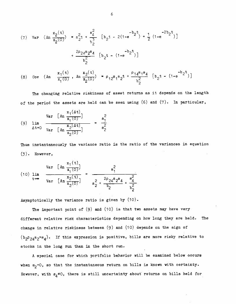
6

x (t) — t —2b t

(7) Var (in x(OP = st + 4_ [bat - 2(1-e2 + (1-e

2

2p ss —bt+

2 [b2t - (1-e )]

x1(t) x2(t) p14s1s4 —b2t(8) Coy (in

x1(0)

in

x2(0)

= +

b[b2t - (1-e )]

The changing relative riskiness of asset returns as it depends on the length

of the period the assets are held can be seen using (6) and (7). In particular,

Var [in 1 2x1(0)

(9) urn (A4-\=

Var [in o 2x2 j

Thus instantaneously the variance ratio is the ratio of the variances in equation

(3). However,

x1(t)Var [in 1 2

(0) Si(io) urn ______________ = _________________t x2tj 2p s

Var [in 1 2 2424 4x2(0) b

22

Asymptotically the variance ratio is given by (10).

The important point of (9) and (10) is that two assets may have very

different relative risk characteristics depending on how long they are held. The

change in relative riskiness between (9) and (10) depends on the sign of

(b2p24s2+s4). If this expression is positive, bills are more risky relative to

stocks in the long run than in the short run.

A special case for which portfolio behavior will be examined below occurs

when 520, so that the instantaneous return on bills is knowii with certainty.

However, with there is still uncertainty about returns on bills held for

7

any finite period. For any given value of the bills are more risky the

smaller the absolute value of b2. For b20, the expected real return on bills

follows a random walk and the asymptotic variance ratio is zero.6

2. The Optimization Problem.

The individual maximizes the expected utility of terminal wealth, WT, where

the utility function is isoelastic:

(11) u(WT)

with =O corresponding to the logarthmic utility function. This class of

utility functions has the important property that the derived utility function in

a dynamic optimization with portfolio rebalancing also belongs to this class,

with the same

The problem to be solved is now the same as that of Goldman (1979), expect

for the different behavior of asset returns. For any given length of holding

period, the investor will maximize the expectation of the derived utility of

wealth function at the end of the holding period. In this isoelastic case, the

derived utility function will be isoelastic with coefficient 3. Thus ignoring

inessential constants, in all cases the portfolio holder faces the problem

x x x-x(12) Max E[(we

1+ (1—w)e 2)/] = E[(we

1 2 + (1—w))e 2/n]

{w}

6Nelson and Schwert (1977), Garbade and Wachtel (1978), and Fama and Gibbons(1982) fail to reject the hypothesis that the real interest rate follows a randomwalk. However, it is not credible that the real interest rate follow such aprocess, which implies the real rate is unbounded above and below.

7The inclusion of consumption possibilities up to time T does not affect resultsso long as the utility of consumption function is also isoelastic with

coefficient .

8

where w is the portfolio share in stocks and and are normally distributed:

(13) N(1, a)

N(t2, o)

cov(x1, x2) a12

It is useful to define

(14) y -x2 N(, a2)

and then note8

(15) E [(we'l 2 + 1_w)e'2/] = E[(we +1_w)Exjy(e2)/p]

=.ç

f (we3T + i—w)e _(Y_(+T))2/2a2dY

where

—

This leads to the first—order condition

(16) 0 = f (we3T + 1_w)_1(e3T_1)e__/2ady

= F(w; y a2...)

Concavity guarantees satisfaction of the second—order condition.

Equation (16) can now be used to study the effects on optimal portfoio

composition of changes in parameters, including the investment horizon.

3. The Goldman Results.

Goldman analyzes the case in which 84=0 so that both asset returns are

8Equation. (is) is used by Goldman (1979) as his canonical form. Multiplicativeconstants are omitted or ignored where no damage results.

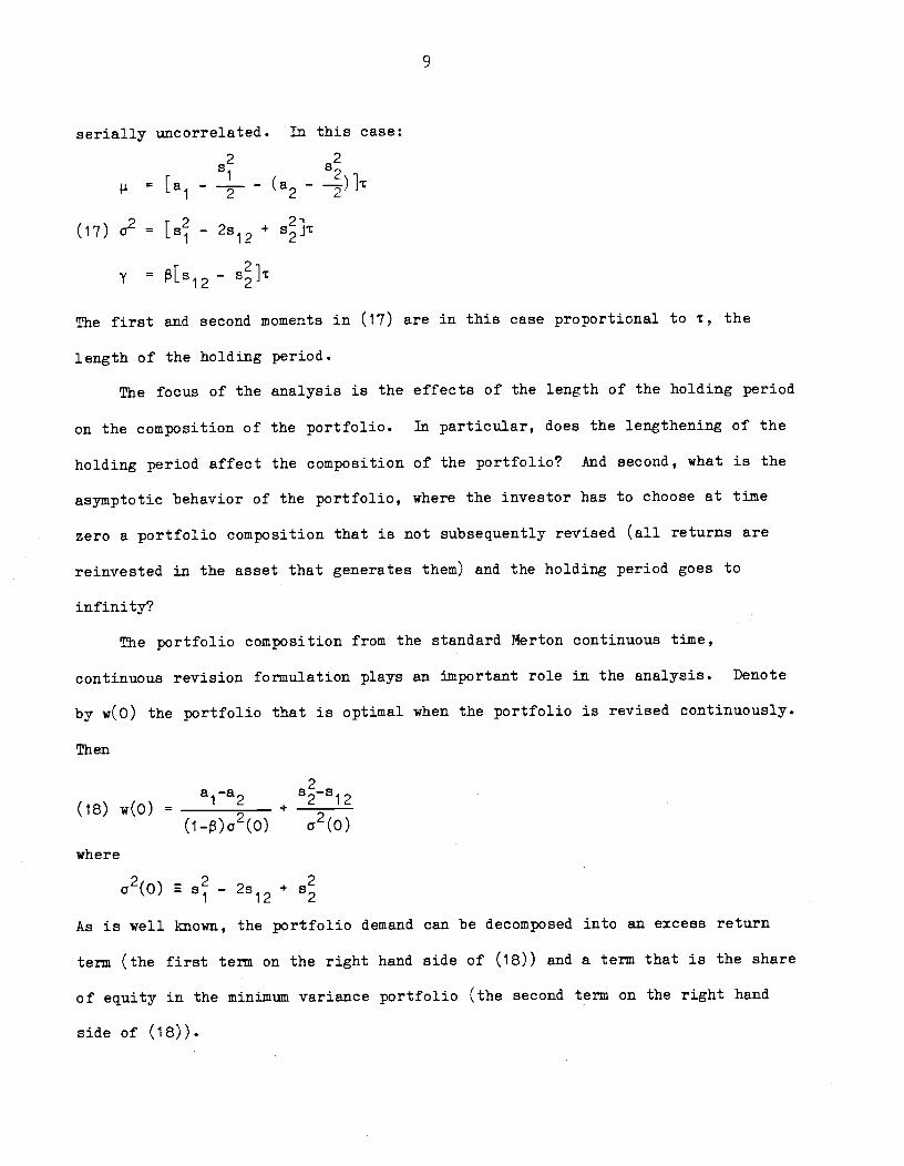
9

serially uncorrelated. In this case:

= [a ——- — (a2

—

(17) 2 = — 2512 + s}rr 2i

I—

The first and second moments in (17) are in this case proportional to r, the

length of the holding period.

The focus of the analysis is the effects of the length of the holding period

on the composition of the portfolio. In particular, does the lengthening of the

holding period affect the composition of the portfolio? And second, what is the

asymptotic behavior of the portfolio, where the investor has to choose at time

zero a portfolio composition that is not subsequently revised (all returns are

reinvested in the asset that generates them) and the holding period goes to

infinity?

The portfolio composition from the standard Nerton continuous time,

continuous revision formulation plays an important role in the analysis. Denote

by w(O) the portfolio that is optimal when the portfolio is revised continuously.

Then

a—a(18) w(O) =

1 2 + 2 12

(1_)a2(O) a2(O)

where

a2(O) s2—2s +

As is well known, the portfolio demand can be decomposed into an excess return

term (the first term on the right hand side of (18)) and a term that is the share

of equity in the minimum variance portfolio (the second term on the right hand

side of (18)).

10

The role played by w(0) in the analysis results from the presence of the

term (+1)/2 in (16). It can be shown that

(19) i = (1-)w(O) - I2

Denoting by w(T) the optimal portfolio when the holding period is of length

Goldman's results can be stated as

G1 If w(O) 0, w('r) = 0

w(0) > 1, w(r) = 1

w(0) = 1/2, w(r) = 1/2

for all ¶

for all ¶

for all ¶.

G2 If 0 < w(0) < 1/2, then (i) dw(r) < 0 and (ii) 0 w() < 1/2

dw("r)1/2 < w(0) < 1, then (i) > 0 and (ii) 1/2 < w(T) ( 1.

then w() = 1/2 [w(0) — 1/2],--p-

otherwise w() = 0 or 1.

11sult G3 is that the portfolio tends asymptotically to plunge to complete

specialization unless the original portfolio composition is nearly balanced. In

that case, as Goldman explains, the distance from 1/2 is magnified by a factor of

These results state that as the

less balanced. If the share of

half, it tends to fall. If the

half, the share tends to rise.

holding period lengthens.

G3 If 1/2 - max (0, 2(i—P

holding period lengthens, the portfolio becomes

stocks is originally positive but less than one

share of stocks is originally greater than one

There is in general antidiversification as the

< w (0) < 1/2 + max (0, 2(1-p)

11

(i—p)/p. For > 0 (utility functions with less risk aversion than the

logarithm) all portfolios plunge asymptotically unless w(O) = 1/2. As tends to

minus infinity, the portfolio tends to stay frozen at its original composition,

which is the variance minimizing portfolio.9

The Goldman results are illustrated in Figure 1, which shows the asymptotic

share of stocks, w(°), as a function of w(0) defined in (ie). In Figure 1 it is

assumed that < 0; for > 0, the ww() locus becomes vertical at w(O) = 1/2,

and then horizontal at w()1. Proposition G2 asserts that the movement away

from w(0) to w() is monotone with the length of the holding period.

4. The Effects of a Change in the Variance of Bill Returns.

As a preliminary to examining the effects of serial correlation of bill

returns on the sensitivity of the portfolio to the length of the holding period,

it is useful to analyze the effects of a change in the variance of bill returns

on the optimal portfolio, w(0), for the continuous portfolio rebalancing, no

serial correlation problem.

from (18):

(20)ôw(0) = w(0) ôo2(O) + 2s2—p12s1

o(O) be2

9G2 and G3 can equivalently be stated as:

G2': If + y + < 0, then < 0 and 0 w(r) < 1/2

+ + > 0, thenbw() > 0 and 1/2 < w() 1

G3': If<0and0<—1<1, thenw()—}..

Otherwise w() = 0 or 1.

Figure 1: AsyrrtotiC (t)

ha

I/

Iw ()

1

.5

•1,

.5 1—23

2(1—s)1

ww ()

w (0)

Share of Stocks

:à—

"

Portfolio (for < 0)

12

2s2(1-.w(O)) D12S1 (2w(D)—1=2

+ ________________

The presumption would be that an increase in the variance of bill returns would,

in this setting, increase the share of stocks in the portfolio. Provided that

portfolio returns are uncorrelated (p120), that is what happens so long as

O<w(O)<1.

However, when it is possible that an increase in the variance of

bill returns reduces the share of stocks in the optimal portfolio. To focus on

- — 4y 1 inc rf (2r +hi+ o_=fl ic

considering the effects of a change from bills being a perfectly safe to a

slightly risky asset.

The effect of the change in s2 then depends on the sign of p12(2w(O)—1). If

then the individual will move away from stocks towards bills when the

riskiness of bills rises, if w(O)<1/2. The reason is that an increase in

increases the riskiness of the portfolio. Someone for whom w(O)<1/2 is

sufficiently concerned about risk to be primarily in bills to begin with. When

the portfolio becomes more risky he seeks the shelter of the relatively safer

asset, which in this case is bills.

If w(O)>1/2, then the individuals response to the increase in the riskiness

of bills and the existing portfolio is to move towardstocks. He thus moves in

the direction of the more risky asset: his tendency to take a relatively risky

position has already been signalled by the fact that his portfolio is

predominantly in stocks.

If p12<0, an increase in the riskiness of bills reduces the overall

riskiness of the portfolio and responses are accordingly the reverse of those

described in the preceeding two paragraphs. Thus in response to an increase in

the riskiness of bills an individual may actually move his portfolio into bills.

The direction of response depends on the factors set out in (20).

13

II. Asymptotic Portfolio Behavior When Returns are Serially Correlated.

We now examine the effects of increases in the length of the holding period

on the optimal portfolio when bill returns are serially correlated. To avoid

unnecessary complexity, s2 is set equal to zero, implying that bill returns for

the next instant are known with certainty. However, s4>O, implying that future

interest rates are not known with certainty.10

Referring back now to (13), (14), and (15), we have in this case

(21) = [a1 — a,, —

—

2 2 2 2 Sl4r 1—ea = — 2a14 + 04 = s1 — 2 LT

2 2

b —2b2T+ —i-- [b - 2(1-e

2 + (1—e )]

b3 2 22

y = (a14-

where 014 and are defined implicitly in the expression for 2, where it is

assumed that a2(0) a2, and where it is understood that p,a2, etc. are

functions of the length of the holding period, r.

Asymptotic portfolio behavior obtains as r, the holding period, goes to

infinity. The share of stocks in this portfolio is denoted (); the "A"

indicates that now there is serial correlation of asset returns. It is

convenient to define

10These are the assumptions made by Merton (1973) in his examination of theeffects of a changing opportunity set on CAPM.

14

2 —2 2 2

(22) i = = a —a2

— ; oi o1/r =2( \ 2—

014(r) s14 0t) s

a1 A= 1un = = 1un ______ =

1 2 b2

and

014 ; ka_cY14

Restating G3 in the form G3' of footnote 9:

G3': If <OadO<-E.<1, then(u)_Otherwise (a) = 0 or 1.

Equivalently

(23) For < 0:

if k < < - h, then () = - ______

- Aif(k, w()O= 1

We now take up in turn the analysis of asymptotic portfolios

(a) for 14 = 0, arid (b) when

(a) When a14 = 0, there is zero correlation between changes in the expected

return on bills and the return on stocks. Main working with w(O) from (18), we

have

2

w(O)[(1-)s] - 81 -(23)() =

2 —2i± 0< w(') < 1, p < 0, and 14 = 0.

+04]

The (a) schedule in Figure 2 describes the relationship (23). The

schedule ww() from gure 1 is included for comparison. The effects of

uncertainty about bill returns are reflected in the 4(°) schedule lying above

15

the ww(a) schedule for all w(O) for which the asymptotic portfolio is diversified

when bill returns are certain.

As drawn, the r() schedule intercepts the vertical axis at positive

The condition that produces the relationship shown in Figure 2 is that

+ < 0. This will happen either if the individual is very risk averse

((—p)large) or if the variance of bill returns is high. As drawn, an individual

who chooses to short stocks (w(0) < 0) when the portfolio is instantly adjustable

may hold positive amounts of stocks if the holding period is very long.

As risk aversion increases, we find

(24) urn w() =—

which is just the variance minimizing share of stocks. Such an individual would

have w(0) 0 since instantaneously bills are riskless.

For > 0, portfolios plunge asymptotically. Modifying G2' of footnote 9,

we have that portfolios plunge to stocks if

—2

(25)—k+-_>O-2 _____where a = lim

t+

Equivalently, for > 0

(25)' (w) = 1 if > (/2)

= 0 if < (p/2) (—s)

Condition (25)' appears paradoxical in that for > o a large or

variance of bill returns, apparently leads to plunging in stocks and vice versa.

iSa

Figure 2: Asvrrtptotic Portfolios Wnen Bill Pturns are Uncertain (l4_0,<0)

A

w (co)

I

I

SS

aSII()

2Si

(1—8) s

.5 1—2 B' .—,

w(O)

16

However, note that the returns on stocks and bills are each log—normally

distributed, implying that the expected excess return per period on stocks is

A -(26) = + -

Then (25)' can be rewritten as:

1— 2 2(25)"For > 0: w() = 1 if >

—_— (s —04)

A 1—s 2 2w() =Oif<—-—(s1 04)

Thus, holding the expected excess return on stocks constant, a smaller

variance of stock returns or larger variance of bill returns tends to lead to

plunging in stocks.

(b) When there is zero correlation between changes in the interest rate and

stock returns, the effects of serial correlation of bill returns on asymptotic

portfolios are almost entirely as expected. The serial correlation of bill

returns makes bills a risky asset for the long term and tends to reduce their

share in the optimal portfolio. Because asset returns are log—normal, though, an

increase in the variance of bill returns increases the expected return on bills.

When the individual is not very risk averse ( > 0), an increase in the variance

of bill returns without any other parameter changing may increase the share of

bills in the portfolio (from zero to one). However, if the expected return on

bills is held constant through an offsetting change in a2, then as (25)" shows,

an increase in uncertainty about bill returns will not increase the share of

bills.

Once correlation of bill and stock returns is introduced, some of the

simplicity disappears. We start again with < 0 a:d allow for in

17

2i 2+ 14 —A(23)'()= 2 — —2 if O(w()(1and<O

-[i - 2a14+

a4]

Now the relationship between Aw(o) and w(O)11 depends on the sign of

Figure 3(a) and 3(b) show the two possibilities. In both cases the schedules

and ww(°) from Figure 2 are included for comparison. When a4 > 0, the

schedule W(°) (schedule for 34*O) is steeper than ww(), and there is a smaller

range of w(O) for which portfolios are diversified asymptotically (compared with

Figure 2).

Comparing (°) in Figure 3(a) with ww(o), it is certainly the case that the

portfolio plunges to stocks on (°') for values of w(O) below (1—2)/2(1—), the

critical value on ww(oo). For (a —a14) < 0, it is also true that the portfolio

plunges to bills on *() for values of w(O) above 1/2(1—n), the critical value

on

Thus the effect of uncertainty about bill returns is certainly to drive

portfolios that are predominantly in stocks further to stocks. However, when

— a1) < 0, portfolios with small holdings of stocks may be driven further

into bills as the variance of bill returns (or serial correlation of bill

returns) increases. The explanation for this latter result is that when

—a14 < 0, the addition of bills to the portfolio substantially reduces the

'1Note we continue to use w(0) from equation (18) as the comparison portfolio.

However, when it is no longer true that (18) gives the portfolio that

would be held if there were continuous rebalancing. Rather, with there is

an additional hedging term in the demand function for the portfolio (o), where"A" indicates the presence of serial correlation of bill returns. (See Merton(1973)). For a14 0, (o) = w(0).

2l 2-74-804

(1—8)

17a

Portfolio With Uncertain Bill Returns (c A > 0, 8 <0)

Figure 3 (b): Asvrrtotic Portfolios With Uncertain Bill Returns (:14 < 0, 8< 0)

j (a,)

1

÷81—8 2

Si

-'1 +__7• 4

(1—8) s

1—282(1—8)

4 14(1—8)

-Fire 3(a): otic

A

w(°')

1P. A

/',M(00)

I 0 I1—28

2(1—8)_N1—28÷ 82(1—8) 1—8

014

Si

18

overall riskiness of the portfolios. If w(O) was low to begin with, then

parameter values were such as to reflect relatively great concern about risk —

which is reduced by adding bills to the portfolio.

Figure 3 (b) describes the asymptotic portfolio when < 0, so that the

expected return on bills is high when stock returns are low. This should be

expected to lead to more diversification, which is precisely what it does. The

relative positions of points A through E in Figure 3(b) are as shown. However B

and A, or just B may be to the right of the origin. Further, point E is shown to

the right of w(O) = 1, but it may be to the left.

The range between points A and E depends in part on the degree of risk

aversion. For (—n) large, A will be at a negative value of w(0) and E will be at

a value of w(O) in excess of unity. In such a case the asymptotic portfolios are

more diversified than w(O). This is the opposite of Goldman's result.

Similarly, the larger in absolute value is a14, (for 14 < 0) the more likely is

the asymptotic portfolio to be diversified for parameter values for which the

portfolio w(0) is not diversified.12

Turning again to asymptotic portfolios for > 0, it turns out that the

discussion of part (a) above applies exactly. Since these portfolios all plunge,

diversification and covariance are not relevant here.

12The question arises of whether this result occurs because w(0) and not (o) isbeing used for comparison. The portfolio 0(o), optimal under the asset dynamicsof this section and with continuous rebalancing is:

w(0) = w(0) +

(1—)s1K

K2/K is a "hedging coefficient", of the same sign as . Thus for < 0 and

< 0, '(o) > w(0). The values of(°) for w(0) < 0 therefore certainlyreiaect portfolio diversification that would not occur even if the comparisonwere w(0), but values of () < 1 for w(0) > 1 may not reflect diversification inexcess of that occurring in the continued rebalancing problem.

iq

(c) Figures 2 and 3, together with (25)" summarize the effects of uncertainty

about bill returns on the asymptotic portfolio. The results are that increased

uncertainty about bill returns increases the share of stocks when 14 = 0; that

when 14 > 0, asymptotic portfolio diversification occurs over a more restricted

range of w(O); and that for 0j4 < 0, the uncertainty about bill returns over the

long term increases the share of stocks for w(O) small and decreases the share of

stocks for w(O) large.

For < 0 and non—plunging portfolios, we can also summarize the above

discussion by using (23) to study the effects of an increase in serial

correlation, or reduction in b2, on the asymptotic portfolio. Since b2 always

enters in the form s4/b2, we can consider the effects of an increase in serialA

correlation on the optimal portfolio by calculating . From (23):54

= (1-())k -

Thus

(27) = 1[2s (i-b)) - p s b (1-2))]

4 b(h+k) 142

Comparing (27) with (20), we note that the effect of an increase in the

serial correlation of bill returns (equivalently an increase in the variance of

bill returns) on the asymptotic share of stocks is precisely the same as that of

an increase in the variance of bill returns on the share of stocks in the

portfolio problem with continuous rebalancing. Thus the ambiguities discussed

following (20) apply here too: for p14 = 0, an increase in the variance of bill

returns unabmiguously increases the share of stocks, (as in Figure 2) but for

it is quite possible that an increase in the variance of bill returns

increases the share of bills. This would happen for instance, if p14 > 0 (Figure

20

3a) if 54 = 0, and the portfolio is predominantly in bills to begin with, 80

1_2(c1) > 0. Alternatively, if p14 < 0 (Figure 3b) and is large, an

increase in 54 may increase the share of stocks. Once more the simplicity of the

Goldman results is lost.

III. Portfolio Behavior with Finite Revision Time Portfolios and Estimated

Return Processes

In general, a closed form solution for the optimal portfolio weight,

cannot be obtained when the revision time, r, is finite, i.e., 0 < < , and

asset returns are serially correlated. However, given values for the coefficient

of relative risk aversion, , and the parameters of the asset returns' stochastic

processes, equations (3) and (4), a numerical solution for '(i) can be found

using equation (16). The form of the integrand of equation (16) is well suited

for applying a Gauss—Hermite quadrature formula. After computing a value for the

integral in (16) for given '(t), we can then iterate over values of (t) until

one is found that satisfies equation (16).

In this section we present calculated optimal portfolios '('r), based on

estimated processes for stock and bill returns. We started by estimating

processes (3) and (4), using weekly data over the period January 1978 to December

1983, a total of 312 weeks. As sho'zn by Tarsh and Rosenfeld (1983), using

returns with a weekly observation interval provides accurate estimates of the

continuous time model parameters of equations (3) and (4) when a discrete time

approximation is used in the estimation process. However, since a price index

series is not available on a weekly basis, equations (3) and (4) are assumed to

describe nominal returns. For the expected rate of return on asset 2, bills, the

annualized yield on outstanding 91 day Treasury Bills with approximately one week

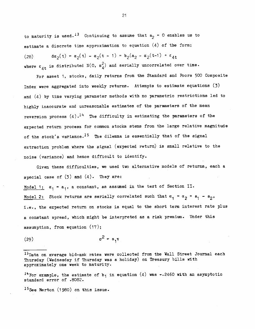
21

to maturity is used.13 Continuing to assume that s2 = 0 enables us to

estimate a discrete time approximation to equation (4) of the form;

(28) da2(t) = a2(t) — a2(t - 1) =b2(a2 - a2(t-l) +

where C4t is distributed N(0, s) and serially uncorrelated over time.

For asset 1, stocks, daily returns from the Standard and Poors 500 Composite

Index were aggregated into weekly returns. Attempts to estimate equations (3)

and (4) by time varying parameter methods with no parametric restrictions led to

highly inaccurate and unreasonable estimates of the parameters of the mean

reversion process (4).1 The difficulty in estimating the parameters of the

expected return process for common stocks stems from the large relative magnitude

of the stock's variance.'5 The dilemma is essentially that of the signal

extraction problem where the signal (expected return) is small relative to the

noise (variance) and hence difficult to identify.

Given these difficulties, we used two alternative models of returns, each a

special case of (3) and (4). They are:

Model 1: a1 = a1, a constant, as assumed in the text of Section II.

Model 2: Stock returns are serially correlated such that =a2

+ a1 — a2,

i.e., the expected return on stocks is equal to the short term interest rate plus

a constant spread, which might be interpreted as a risk premium. Under this

assumption, from equation (17);

(29)=

13Data on average bid—ask rates were collected from the Wall Street Journal eachThursday (Wednesday if Thursday was a holiday) on Treasury bills withapproximately one week to maturity.

Por example, the estimate of b1 in equation (4) was —.2460 with an asymptoticstandard error of .8082.

15See Merton (1980) on this issue.

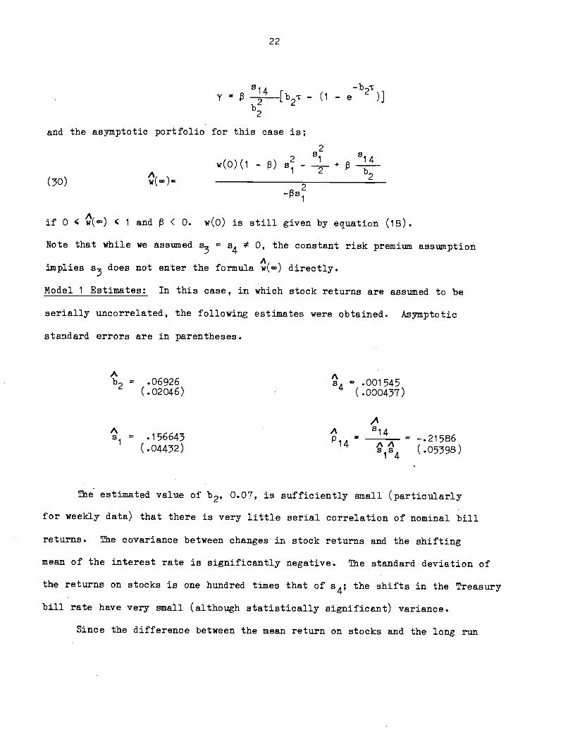
22

-b=

2 {b2r - (i - e 2

b2

and the asymptotic portfolio for this case is;

2

w(0)(i2 1

+ 14

(30) (a)=1

2

2b2

—s

if 0 ( ( 1 and. < 0. w(O) is still given by equation (18).

Note that while we assumed83 84

0, the constant risk premium assumption

Aimplies 83 does not enter the formula w() directly.

Model 1 Estimates: In this case, in which stock returns are assumed to be

serially uncorrelated, the following estimates were obtained. Asymptotic

standard errors are in parentheses.

A A= .06926 84 = .001545(.o2o46) (.000437)

AA A 14s = .156643 p = ______ = —.21586

(.04432) 51s4 (.os)

The estimated value of 2' 0.07, is sufficiently small (particularly

for weekly data) that there is very little serial correlation of nominal bill

returns. The covariance between changes in stock returns and the shifting

mean of the interest rate is significantly negative. The standard deviation of

the returns on stocks is one hundred times that of s4; the shifts in the Treasury

bill rate have very small (although statistically significant) variance.

Since the difference between the mean return on stocks and the long run

23

expected return on bills, a1 — a2 can only be estimated with reasonable

accuracy by using data over a long time period, an estimate of the spread was

obtained from Ibbotson and Sinquefield (1982). The means of Standard and

Poors stock returns and Treasury bill returns over the period 1926-1981 were a1 =

.114 and a2 = .031, so we take the estimate of the spread to be .083.

Model 2 Estimates: For the alternative case in which stocks are serially

Acorrelated and a1 = a2 +

a1— a2 we have the following estimates (b2 and 84

are the same in the two models):

AA A 14a = .156667 p1 = _____ = —.21513

(.04433) Sj84 (.05399)

These are very similar to the Model 1 estimates of these same parameters.

Calculated Portfolios: We computed finite revision time portfolio weights

using the point estimates for the returns processes of Models 1 and 2.

Results for Model 1, with serially uncorrelated returns on stocks, are

presented in Table 2 while Model 2 results appear in Table 3. (In the w(x)

expressions, x is measured in years.) The calculated portfolios are very

similar in the two tables. The results are:

1. For coefficients of relative risk aversion of 0, -1 (the logarithmic

utility function) and —2, the optimal portfolio weights are all equal to 1

and are not reported in the tables.'6

2. The optimal portfolio weights change little with the length of the

portfolio revision period. Most of the change occurs after ¶ = 10 years.

161f bills and stocks were the only assets held in the portfolio, then wecould estimate the coefficient of relative risk aversion by finding thatvalue of for which the calculated portfolio proportions were equal to theactual.

24

3. The Goldman plunging results are not applicable over the ranges seen in

the tables. Indeed, with the serial correlation of bill returns, there are

for high values of — movements towards diversification as the holding period

lengthens. In all cases the w(T) portfolio contains more stocks than the

w(O) portfolio. This is in accord with the Goldman anti—diversification

results for values of greater than —6; for < —6, the Goldman anti-

diversification and the greater relative riskiness of bills effect stressed

in this paper work in the opposite direction. Asymptotically the increasing

relative riskiness of bills effect dominates anti—diversification, but the

change is not monotonic.

4. The difference between the (O) and w'(O) portfolios is zero to five

places. This means that hedging effects on portfolio demands are negligible

for the processes examined in this paper. That is not surprising given the

small estimates of the serial correlation of bill returns. If such estimates

are reliable, the one period CAPM provides a close approximation to the CAPM

with a changing opportunity set.

An Alternative "Safe" Asset: We calculated optimal portfolios with one week

bills replaced by 91 day bills. With asset 2 a 91 day bill, 2 is not equal

to zero. For this case equation (3) was estimated using weekly new issue

auction yields on 91 day Treasury bills over the same period as before,

January 1978 to December 1983. The expected return was assumed equal to a

proportion of the short rate used previously in estimating (28) plus a

constant. This assumption concerning the form of the stochastic process of

Treasury bills is consistent with the term structure model of Vasicek (1977).

The following point estimates were obtained for the case (Model 1) in which

stock returns were assumed to be serially uncorrelated.

25

= .0103235 12 = .20655 = —.391372 (.0029211) (.05419) (.04794)

The following alternative estimates were obtained for the case (Model

2) in which stock returns were assumed to be serially correlated.

p12 = .20584 p14= -.21513

(.05422) (.05399)

The model in which 2 * 0 requires a straightforward modification of the

formulas for p., cr2, and y which can be made using equations (7) and (8).

We again calculated solutions for (t) using equation (16). Table 4

presents the optimal stock holdings for the case in which stocks are assumed to

be serially uncorrelated. Qualitatively, the results for this case for which the

maturity of asset two has been extended are very similar to the results in Table

2 where asset two is the short (i week) rate.

Essentially the same situation is found when stock returns are assumed

to be serially correlated. The results in Table 5 give @r) for serially

correlated stock returns and asset two being 91 day bills. The monotonicity

results of Goldman (1979) again do not hold. As in Tables 2 and 3 there is very

little change in magnitude between w(0) and

Estimation Using Real Asset Returns: Models 1 and 2 were re—estimated using real

returns data and a monthly observation interval. Equations (3) and (4) are

perhaps a more attractive returns generating process when returns are assumed to

be in real terms rather than nominal. However, the use of returns constrains us

to use a monthly observation interval which may decrease the accuracy of the

parameter estimates.

Treasury bill and. common stock returns, deflated by the CPI, were obtained

from the Ibbotson and Sinquefield bond file over the period 1926 to 1983, a total

26

of 696 observations. Estimation of equation (4) for real bill returns yielded

the following estimates.

A A= .47323 s4 = .017501(.03231) (.004053)

For the case in which real stock returns are serially uncorrelated

(Model 1), the following estimates were computed.

A A= .20749 p14 = —.05872(.04806) (.03780)

Similar estimates were obtained under the alternative assumption that real

stock returns are correlated (Model 2).

A As = .20703 p1

= —. 05889(.04795) (.03780)

Using real monthly returns instead of nominal weekly returns results in bill

Areturns having higher serial correlation (b2 = .47323), though the correlation

between stocks and bills is smaller. Also, using a longer period (1926—83), we

find that the standard deviations of real stock and bill returns, .207 end .018,

respectively, are larger than the corresponding nominal stock and bill return

standard deviation estimates over the 1978—83 period, .157 and .010.

Tables 6 and 7 give the optimal stock portfolio weight, (t), for Model 1

and Model 2, respectively. The estimates in both of the Tables are quite

similar. The larger estimated variance of stocks seems to have the effect of

reducing the optimal portfolio weights compared to those estimated in Tables 2

and 5. However, there continues to be very little difference between the

continuous revision portfolios for the non—serial correlation case, w(0), and the

serial correlation case, (o). Also as in previous estimates, there is not

generally monotonic anti—diversification as the revision period increases, though

there continues to be little difference in optimal portfolio weights even out to

a 10 year revision interval.

27

IV. Conclusions

The notion that portfolio behavior might depend on the length of time

for which the portfolio is held is highly intuitive. Goldman (1979) showed

that the relevant period is not the investor's horizon, but rather the

portfolio revision period, the length of time for which the portfolio cannot

be revised. Assuming serially uncorrelated asset returns Goldman proved an

anti—diversification result, in which the portfolio becomes less diversified

— as the portfolio revision period increases.

When asset returns are serially correlated, the relative riskiness of

assets is typically a function of the length of time for which they are held.

We show in this paper how changes in the relative riskiness of assets

interact with changes in the portfolio revision period to affect portfolios.

The Goldman anti—diversification result no longer necessarily holds. Nor is

the change in the portfolio any longer necessarily a monotonic function of

the length of the portfolio revision period.

We estimated dynamic processes for bill and stock returns, and used them

to calculate optimal portfolios as a function of the portfolio revision

period. The most striking result was how little the portfolio proportions

changed as the period lengthened. We did find in cases where the Goldman

anti—diversification tendency conflicted with changing relative variances of

asset returns, that the changing relative variances were asymptotically

dominant.

Because the serial correlation of asset returns was estimated to be

relatively low, there was very little difference between portfolios estimated

with and without hedging demands. If our estimated processes are reasonably

accurate, hedging demands and the errors made in assuming a one—period rather

than multi—period CAPN are small.

28

It remains entirely possible that individual assets, like land and

particular stocks, could display considerable serial correlation of returns

despite the absence of significant serial correlation of asset returns at the

aggregate level.

Table 1: Real Monthly Returns on Stocks and Bills

Period

Notes: 1. The variances should all be multiplied by .01.

2. Stock and bill returns are from the Ibbotson—Sinquefield File, Centerfor Research in Security Prices, University of Chicago. Real returnsare calculated using the Consumer Price Index.

3. Parentheses in last row of table are a reminder that statistics arebased on only eleven and seven data points respectively.

1926—1983 1948—1983

(1) (2) (3)

Stocks Bills (1)/(2)(1) (2) (3)

Stocks Bills (1)/(2)

.00687Mean return

Variance ofreturns per monthW

Holding periodin months:

.0001145 .00656 .0003140

1 .352 .00356 98.6

2 .1411 .00553 714.3

'4 •31414 .008142 140.9

12 .372 .01712 21.7

60 (.259 .05023 5.2)

.163 .00119 137.0

.168 .00168 100.0

.162 .002814 57.0

.250 .00620 40.3

(.287 .00821 314.8)

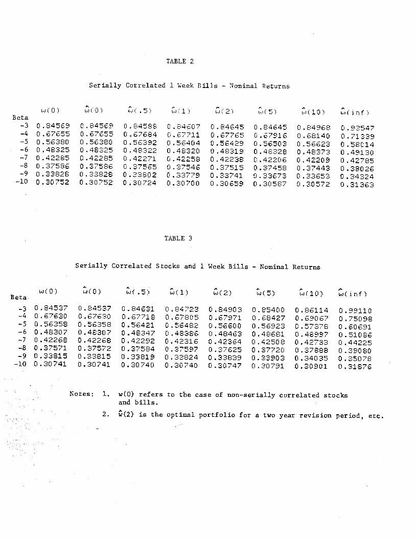
TABLE 2

Serially Cotrelated 1 Week Bills — Nominal Returns

Serially Correlated Stocks and 1 Week Bills — Nominal Returns

Notes: 1. w(0) refers to the case of non—serially correlated stocksand bills.

2. (2) is the optimal portfolio for a two year revision period, etc.

Beta

•S0) ':0) A&'( .5: .* 2 (5 •) 10 c• i n f

-3 0 .84569 0 . 84559 0 . 84588 0 . 8407 0 .84645 0 . 84645 0 . 8468 0 547—4 0.67655 0.67655 0.67684 0.67711 0.67765 0.57916 0.68140

.

0.71339-5 0.56380 0.56380 0.56392 0.56404 0.55429 0.55503 0.56523 0.58014-6 0 .48325 0 .48325 0 .48322 0 .48320 0 .48319 0 .48328 0 .48373 0 .49130—7 0 . 42285 0 . 42285 0 . 42271 0 .42258 0 .42238 0 . 42205 0 . 42209 0 .42785-8 0.37586 0.37585 0.37565 0.37546 0.37515 0.37458 0.37443 0.38025-9 0 . 33828 0 . 33828 0 .33802 0 . 33779 0 .33741 0 . 33673 0 33653 0 .34324

—10 0.30752 0.30752 0.30724 0.30700 0.30659 0.30587 0.30572

TABLE 3

Beta.',.i(O) wCO) w( .s: (2) w(10) w(inf)

0.84527 0.84537 0.84631 0.84723 0.84903 0.85400 0.86114 0.99110-4 0.67630 0.67630 0.67718 0.67805 0.57971 0.68427 0.69057 0.75098-5 0.55358 0.56358 0.56421 0.55482 0.56600 0.56923 0.57378 0.60691-6 0.48307 0.48307 0.48347 0.48386 0.48463 0.48681 0.48997 0.51086-7 0.42268 0.42268 0.42292 0.42315 0.42364 0.42508 0.42733 0.44225-8 0.37571 0.37572 0.37584 0.27597 0.37625 0.37720 0.37888 0.39080-9 0.33815 0.33815 0.33819 0.33824 0.33839 0.33903 0.34035 0.35078—10 0.30741 0 .30741 0.30740 0.30740 0. 30747 0.30791 0

Serially Correlated Stocks and 3 Month Bills — Nominal Returns

Notes: 1. w(0) refers to the case of non—serially correlated stocksand bills

2. (2) is the optimal portfolio for a two year revision period, etc.

TABLE 4

Serially Correlated 3 Month Bills — Nominal Returns

w (Ci),.w':°O:

.w .5) w(1) w(2) ..t(5) ..w(l0) ,.':irf)Beta

—3 0.85601 0.35501 0.85514-4 0.68291 0.68291 0.68315-5 0.56751 0.55751 0.55759-6 0.48508 0.48503 0.48500-7 0.42326 0.42226 0.42306-8 0.37518 0.37518 0.37490

—c.

• , J. rJ • —, _, f . r ''CiJ . ,_j _J '— —

—10 0.30524 0.30524 0.30489

0.85529 0.85658 0.85753 0.85924 0.947250.53340 0.53387 0.68518 0.58716 0.718610.55767 0.55784 0.56835 0.55922 0.581430 .48493 0 . 48481 0 - 48453 Ci . 48469 0 . 489970.42288 0.42257 0.42193 0.42153 0.424540 .37465 0 .37421 0 . 37331 0 . 37268 0 .375550.33610 0.23559 0.33455 0.33385 0.337540.30457 0.30403 0.3029? 0.30227 0.30706

TABLE 5

wCO) (0) w(.5) w(1) w(2) w(5)-..w(10) .i(inf)

Beta-3 0.85564 0.85564 0.35552 0.85738 0.85905 0.86369 0.87038 1.00000—4 0.68262 0.63263 0.58347 0.68430 0.58589 0.69024 0.69636 0.75586-5 0.56728 0.56728 0.55787 0.56845 0.5G956 0.57259 0.57685 .0.60831—6 0.48489 0.48489 0.48526 0.43561 0.48631 0.48327 0.49112 0.50995-7 0.42310 0.42310 0.42330 0.42350 0.42390 0.42512 0.42703 0.43959-8 . 0.37504 0.37504 0.37512 0.37521 0.37541 0.37613 0.37747 0.38700-9 0.33660 0.33660 0.33650 0.33661 0.33668 0.33708 0.33305 0.34601

—10 0.30514 0.30514 0.30509 0.30505 0.30504 0.30524 0.30599 0.31322

TABLE 6

Serially Correlated 3 Month Bills — Real Returns

Serially Correlated Stocks and 3 Month Bills — Real Returns

Notes: 1. w(O) refers to the case of non—serially correlated stocks andbills

2. (2) is the optiinal portfolio for a two year revision period, etc.

w (0) W ( 0 ' .5) t(1 ) CI(5) w(lO ( irif)0.93724 0.93724 0.93570 0.93620 0.93542 0.93501 0.93772 1.000000.62482 0.62482 0.62526 0.62587 0.62731 0.63165 0.63711 0.692950.46862 0.46862 0.46873 0.46912 0.47026 0.47346 0.47595 0.475340.37489 0.37489 0.37483 0.37512 0.37614 0.37892 0.38022 0.366540.31241 0.31241 0.31230 0.31259 0.31366 0.31653 0.31756 0.301250.26778 0.26778 0.26769 0.26803 0.26924 0.27241 0.27356 0.257730.23431 0.23431 0.23427 0.23469 0.23606 0.23960 0.24105 0.225640.20827 0.20827 0.20830 0.20880 0.21034 0.21428 0.21607 0.203330.18745 0.18745 0.18755 0.18812 0.18983 0.19415 0.19629 0.185190.17041 0.17041 0.17058 0.17123 0.17309 0.17777 0.18024 0.17069

TABLE 7

Beta

—l—2—3—4—5—6—7—8

—9—10

Beta

—l—2—3—4—5—6—7—8—9—10

w(0) (0) (.5) i(1) '(2) '(1O) '(inf)0.941410 . 62760o .470700 . 376560 .313800.268970 . 235350.209200 .188280.17116

0.941410 . 627600.470400.376560.313800 .268970.235350.209200.188280.17116

o . 942500 .629000.471420 . 376880.313930.269020.235370 .209230.138330.17125

0 . 943490 .530270.472030.377110.313980.26898nU •0.209180.188300.17124

0 . 945250 . 632510.472980.377350.313870 . 268740 .235020.208890.188050.17105

0 . 949350 . 637540 . 474510.377050 .31273O . 267240 . 233430.207330.186590.16970

0 .954310.543110 . 475230 . 375440.310130 .254280.230390.204360.183760.16704

1.000000.701920.471460 . 356220.287080.240990.208060.183370.164160.14880

29

References

Fama, Eugene and Michael Gibbons (1982); "Inflation, Real Returns and Capital

Investment", Journal of Monetary Economics, 9 (May): 297—324.

Fischer, Stanley (1983); "Investing for the Short and the Long Term", in Z.

Bodie and J. Shoven (eds.); Financial Aspects of the United States

Pension System, Chicago: University of Chicago Press.

Garbade, Kenneth and Paul Wachtel (1978); "Time Variation in the Relationshipbetween Inflation and Interest Rates", Journal of Monetary Economics, 4

(November): 755—66.

Goldman, Barry M. (1979); "Anti—diversification, or Optimal Programs forInfrequently Revised Portfolios", Journal of Finance, 34 (Nay): 505—16.

Ibbotson, Roger G. and Rex A. Sinquefield, (1982), "Stocks, Bonds, Bills andInflation: The Past and the Pature," The Financial Analysts Research

Foundation, Charlottesville, Virginia.

Klein, Benjamin (1976); "The Social Costs of the Recent Inflation: theMirage of Steady 'Anticipated' Inflation", in Carnegie — RochesterConference Series on Public Policy, Vol. 3, Institutional Arrangementsand the Inflation Problem, Amsterdam: North—Holland.

Marsh, Terry A. and Eric R. Rosenfeld (1983); "Nontrading and Discrete Time

Arproximation Errors in the Estimation of Continuous Time Models in

Finance", mimeo, MIT, November.

Merton, Robert C., (1973), "An Intertemporal Capital Asset Pricing Model,"Econornetrica, 41 (Sept.) 867—888.

___________ (1980); "On Estimating the Expected Return on the Market", Journalof Financial Economics, 8: 323—61.

Mossin, J. (1968); "Optimal Multiperiod Portfolio Policies", Journal of

Business 41: 215—29.

Nelson, Charles R. and William Schwert (1977); "Oia Testing the Hypothesisthat the Real Rate of Interest is Constant", American Economic Review

67 (June): 478—86.

Saniuelson, Paul A. (1969); "Portfolio Selection by Dynamic StochasticProgramming", Review of Economics and Statistics, 60 (August): 239—46.

Vasicek, Oldrich (1977) "An Equilibrium Characterization of the TermStructure," Journal of Financial Economics, 5, 117—188.