stanford law revie · 2016-06-04 · 1323 article race, place, and power nicholas o....
TRANSCRIPT

1323
ARTICLE
Race, Place, and Power
Nicholas O. Stephanopoulos*
Abstract. A generation ago, the Supreme Court upended the voting rights world. In the breakthrough case of Thornburg v. Gingles, the Court held that minority groups that are residentially segregated and electorally polarized are entitled to districts in which they can elect their preferred candidates. But while the legal standard for vote dilution has been clear ever since, the real-world impact of the Court’s decision has remained a mystery. Scholars have failed to answer basic empirical questions about the operation of the Gingles framework. To wit: Did minorities’ descriptive representation improve due to the case? If so, did this improvement come about through the mechanisms—racial segregation and polarization—contemplated by the Court? And is there a tradeoff between minorities’ descriptive and substantive representation, or can both be raised in tandem?
In this Article, I tackle these questions using a series of novel datasets. For the first time, I am able to quantify all of Gingles’1s elements: racial segregation and polarization, and descriptive and substantive representation. I am also able to track them at the state legislative level, over the entire modern redistricting era, and for black and Hispanic voters. Compared to the cross-sectional congressional studies of black representation that form the bulk of the literature, these features provide far more analytical leverage.
I find that the proportion of black legislators in the South rose precipitously after the Court’s intervention. But neither this proportion in the non-South, nor the share of Hispanic legislators nationwide, increased much. I also find that Gingles worked exactly as intended for segregated and polarized black populations. These groups now elect many more of their preferred candidates than they did prior to the decision. But this progress has not materialized for Hispanics, suggesting that their votes often continue to be diluted. Lastly, I find a modest tradeoff between minorities’ descriptive representation and both the share of seats held by Democrats and the liberalism of the median legislator. But this tradeoff disappears when Democrats are responsible for redistricting, and it intensifies
* Assistant Professor of Law, University of Chicago Law School. I am grateful to several people for assisting me with this Article’s empirical analysis: John Fahrenbach for helping me to calculate spatial segregation, Carl Klarner for helping me to collect data on black and Hispanic representation, John Ray for helping me to perform multilevel regression and poststratification, and Sumitra Badrinathan for superb overall research assistance. For valuable comments, I thank Adam Chilton, Chandler Davidson, Christopher Elmendorf, Bernard Grofman, Zoltan Hajnal, Ellen Katz, Michael Pitts, Bertrall Ross, Kenneth Shotts, Doug Spencer, Ebonya Washington, and workshop participants at Ohio State, Stanford, Wisconsin, and the Midwest Political Science Association Annual Conference. I am pleased as well to acknowledge the support of the Robert Helman Law and Public Policy Fund.
Volume 68 June 2016
Stanford Law Review

Race, Place, and Power 68 STAN. L. REV. 1323 (2016)
1324
when Republicans are in charge. In combination, these results provide fodder for both Gingles1’s advocates and its critics. More importantly, they mean that the decision’s impact can finally be assessed empirically.
Table of Contents
Introduction ......................................................................................................................................................... 1325
I. Prongs and Puzzles ................................................................................................................................. 1332 A. The Gingles Framework ............................................................................................................ 1333 B. Unanswered Questions .............................................................................................................. 1339
II. Racial Segregation................................................................................................................................... 1342 A. Hypotheses ........................................................................................................................................ 1342 B. Trends ................................................................................................................................................. 1345
III. Racial Polarization ................................................................................................................................. 1349 A. Hypotheses ........................................................................................................................................ 1349 B. Trends ................................................................................................................................................. 1354 C. Drivers ................................................................................................................................................ 1359
IV. Descriptive Representation ............................................................................................................... 1361 A. Hypotheses ........................................................................................................................................ 1362 B. Trends ................................................................................................................................................. 1367 C. Drivers ................................................................................................................................................ 1371
V. Substantive Representation .............................................................................................................. 1380 A. Hypotheses ........................................................................................................................................ 1381 B. Trends ................................................................................................................................................. 1386 C. Drivers ................................................................................................................................................ 1388
VI. Implications ................................................................................................................................................ 1393 A. Positive ................................................................................................................................................ 1394 B. Negative ............................................................................................................................................. 1396 C. Extensions ......................................................................................................................................... 1398
Conclusion ............................................................................................................................................................. 1403
Appendix ................................................................................................................................................................ 1405

Race, Place, and Power 68 STAN. L. REV. 1323 (2016)
1325
Introduction
Senator Orrin Hatch led the opposition to the 1982 amendments that transformed the Voting Rights Act—and with it, minority representation in America.1 The amendments converted what had been a conventional discriminatory intent provision into a far-reaching “results test.”2 Any practice that “results in a denial or abridgement of the right . . . to vote on account of race” became unlawful, regardless of the practice’s motivation.3 Throughout the congressional debate, Hatch hammered a single point. If the results test was not meant to require proportional representation for minority groups (as its backers pledged4), then the test had no “ultimate core value.”5 It “provide[d] absolutely no intelligible guidance to courts in determining whether or not a . . . violation ha[d] been established.”6 It was an empty shell.
The amendments’ supporters were unable to counter Hatch’s criticism. They could not identify an “ultimate core value” (other than proportional representation) underlying the results test. Instead, they resorted to invocations of precedent, claiming it showed that the test could be fairly applied. As the Senate Report put it, “There is . . . an extensive, reliable and reassuring track record of court decisions using the very standard which the Committee bill would codify.”7 In other words, the supporters could not explain how their proposal would operate—but they were confident the courts had already figured it out.
In fact, the courts had done nothing of the kind. The pre-1982 case law on racial vote dilution (the reduction of minorities’ electoral influence through means other than outright disenfranchisement) was a mess.8 It featured a dozen
1. See Voting Rights Act Amendments of 1982 § 2, 52 U.S.C. § 10301 (2014). 2. The Supreme Court had previously construed this section of the Voting Rights Act as
“simply restat[ing] the prohibitions already contained in the Fifteenth Amendment”—and thus requiring discriminatory intent to be proven—in City of Mobile v. Bolden, 446 U.S. 55, 61 (1980) (plurality opinion).
3. 52 U.S.C. § 10301(a) (emphasis added). 4. See, e.g., S. REP. NO. 97-417, at 16 (1982) (“[L]ack of proportional representation is not
enough to invalidate [an] election method.”); id. at 33 (noting the “rejection of proportional representation as the standard for legality under the results test”).
5. Id. at 96. 6. Id. at 99; see also, e.g., id. at 100 (“[H]ow does a community, and how does a court, know
what is right and wrong under the results standard? . . . How do they know which laws and procedures are valid, and under what circumstances, and which are invalid?”).
7. Id. at 32; see also, e.g., id. at 31 (“The proposed results test was developed by the Supreme Court and followed in nearly two dozen cases by the lower federal courts. The results test is well-known to federal judges.”).
8. See, e.g., Christopher S. Elmendorf et al., Racially Polarized Voting, 83 U. CHI. L. REV. (forthcoming June 2016) (manuscript at 9) (on file with author) (referring to the “non-exhaustive list of factors” considered by “the constitutional vote dilution jurisprudence
footnote continued on next page
Race, Place, and Power 68 STAN. L. REV. 1323 (2016)
1326
or so factors that judges balanced as they saw fit, weighing each element based on their own discretionary judgment.9 It offered no “intelligible guidance” except to consider the totality of circumstances.
In the face of this confusion, it fell to the Supreme Court to fashion the results test into a more determinate inquiry. The Court famously did so in the 1986 case of Thornburg v. Gingles, its first encounter with the revised statute.10 First, the Court held that the law aimed to provide descriptive representation to minority voters—or more precisely, representation by minority voters’ candidates of choice. “The essence of a [Voting Rights Act] claim,” the Court declared, “is that a certain electoral . . . practice . . . interacts with social and historical conditions” to prevent minority voters from being able “to elect their preferred representatives.”11
Second, and even more crucially, the Court clarified how much representation minority voters were due. Not maximal representation: the most an electoral system could possibly deliver to them. And not proportional representation either: a share of seats equivalent to a minority’s share of the population. Instead, under the Court’s new framework, a minority group was entitled to elect its preferred candidates only if it met a series of preconditions. It had to be “sufficiently large and geographically compact” to constitute a local majority.12 It had to be “politically cohesive” in its voting preferences.13 And it had to be confronted by consistent “bloc” voting by the “white majority.”14
The Court’s answer to Hatch, then, was this: The results test is neither a mandate for proportional representation nor a blank slate. Rather, it requires for minority groups the level of representation that corresponds to their size, segregation, and polarization. Groups that are geographically compact (that is, segregated) and different from the white majority in their voting preferences (that is, polarized) must be able to elect the candidates of their choice. But
of the 1970s”); Samuel Issacharoff, Polarized Voting and the Political Process11: The Transformation of Voting Rights Jurisprudence, 90 MICH. L. REV. 1833, 1844 (1992) (noting the “absence of an overriding conception of the precise constitutional harm the courts were seeking to remedy” in the pre-1982 period).
9. The two best-known cases setting forth this mélange of factors were White v. Regester, 412 U.S. 755, 765-70 (1973), and Zimmer v. McKeithen, 485 F.2d 1297, 1305-07 (5th Cir. 1973).
10. 478 U.S. 30 (1986); see also, e.g., Heather K. Gerken, Understanding the Right to an Undiluted Vote, 114 HARV. L. REV. 1663, 1674 (2001) (referring to Gingles as a “seminal decision that has dramatically affected voting rights jurisprudence”); Richard H. Pildes, The Decline of Legally Mandated Minority Representation, 68 OHIO ST. L.J. 1139, 1159 (2007) (noting the academic consensus that “Gingles provided the basic framework for giving content to the concept of vote dilution”).
11. Gingles, 478 U.S. at 47. 12. Id. at 50. 13. Id. at 51. 14. Id.
Race, Place, and Power 68 STAN. L. REV. 1323 (2016)
1327
groups that are spatially integrated or electorally indistinct have no such entitlement.
This answer, it is true, supplies the “ultimate core value” sought by Hatch.15 But it raises a host of vexing questions of its own. Some of these questions are normative, and legions of scholars have strived diligently to address them.16 Some of the questions, though, are empirical, and as to them the academy has been remiss. Almost three decades after Gingles was decided, not enough is known about the phenomena the case recognized or the relationships between them. An entire doctrinal edifice has been erected on an uncertain factual foundation.
To start, take the two key determinants of minority representation under the Court’s approach: racial segregation and racial polarization in voting. A large sociological literature has found that black-white segregation is falling at the metropolitan level.17 But what is happening to it (and to Hispanic-white segregation) at the level that matters even more for minority clout: the level of the state as a whole? Similarly, several political science studies have determined that black-white polarization declined modestly in the 1990s.18 But what were its trends (and those of Hispanic-white polarization) before and after this decade? And is the Court right to think that desegregation might fuel depolarization—that we might be progressing toward “a society where integration and color-blindness are . . . simple facts of life”?19
Next consider Gingles1’s overarching goal: the election (if its preconditions are satisfied) of minority voters’ preferred candidates. The number of black and Hispanic members of Congress surged in the 1990s, the first redistricting cycle after the enactment of the 1982 amendments.20 But what about the presence of minority politicians in the state legislative chambers that are the building blocks of American democracy? Did it increase as well, and if so, were these gains sustained in the wake of the Court’s racial gerrymandering decisions, which some feared would decimate minority representation?21
15. See BERNARD GROFMAN ET AL., MINORITY REPRESENTATION AND THE QUEST FOR VOTING EQUALITY 60 (1992) (commenting that in Gingles the Court “constructed a standard that contains a ‘core’ value”).
16. For a recent summary of academic approaches to the Voting Rights Act, see Elmendorf et al., supra note 8 (manuscript at 36-42).
17. See infra Part II.A; see also Nicholas O. Stephanopoulos, Civil Rights in a Desegregating America, 83 U. CHI. L. REV. (forthcoming Sept. 2016) (manuscript at 11-15) (on file with author) (summarizing the trends in racial segregation).
18. See infra Part III.A. 19. Georgia v. Ashcroft, 539 U.S. 461, 490-91 (2003). 20. See infra Part IV.A. 21. Shaw v. Reno, 509 U.S. 630 (1993), was the first of these decisions, which subjected
districts drawn for predominantly racial reasons to heightened scrutiny. For the most famous expression of concern about the decisions’ consequences for minority
footnote continued on next page
Race, Place, and Power 68 STAN. L. REV. 1323 (2016)
1328
Still more interestingly, Gingles connected the election of minorities’ candidates of choice to segregation and polarization in ways the phenomena had not previously been tied. Did this linkage make a difference? That is, did the relationship between segregation and polarization on the one hand, and minority representation on the other, change as a result of Gingles? And if it did, could the relationship be evolving once again as (according to the Court) “integration and color-blindness” increasingly become “facts of life”?22 Put more bluntly, could desegregation or depolarization now be leading to the election of fewer minority-preferred candidates?
Lastly, while Gingles stressed descriptive representation, it also evinced concern for substantive representation: legislatures that, as bodies, promote minorities’ policy interests. Under the decision, “a significant lack of responsiveness on the part of elected officials to the particularized needs of the members of the minority group” is a factor that cuts in favor of liability.23 At the federal level, it is reasonably clear that a tradeoff exists between descriptive and substantive representation, at least for blacks. When more blacks are elected to Congress, fewer Democrats win seats, and the chamber’s median moves in a conservative direction.24 But does this tradeoff apply at the state legislative level too, and for all minority groups, not just blacks? And if so, is the tradeoff unavoidable or can it be mitigated—for instance by Democratic rather than Republican control of redistricting?
There is a reason why these questions have not yet been answered. It is that the information necessary to grapple with them has been absent. To date, no datasets have been compiled of segregation or polarization by state and over time. Even longitudinal estimates of descriptive representation and party vote share have not been produced at the state legislative level. This lack of evidence explains why basic doubts about Gingles—and its “ultimate core value” for the results test—persist a generation after the case was decided.
In this Article, I exploit a series of original datasets to tackle these issues. As to segregation, I used information on the racial makeup and geographic location of all census tracts over a five-decade span to calculate what is known as the spatial index of dissimilarity.25 This is the first time that spatial segregation scores have been computed for states. As to polarization, I relied on the results of all available general election exit polls, including more than 1.2 million respondents, to determine racial differences in vote choice and
representation, see Steven A. Holmes, Court Hears Challenges to Black Districts, N.Y. TIMES (Apr. 20, 1995), http://nyti.ms/1Lj19xi (quoting Eric Schnapper as stating that, due to the decisions, “the Congressional Black Caucus ‘will be able to meet in the back of a taxi cab’”).
22. Ashcroft, 539 U.S. at 490-91. 23. Thornburg v. Gingles, 478 U.S. 30, 37 (1986) (quoting S. REP. NO. 97-417, at 29 (1982)). 24. See infra Part V.A. 25. See infra Part II.B.

Race, Place, and Power 68 STAN. L. REV. 1323 (2016)
1329
political ideology.26 Whenever state-specific polls were not conducted, I employed a new statistical technique to derive state-level estimates from the national polling data.27
As to descriptive representation, I consulted a range of sources to track the number of black and Hispanic state house members by state and year.28 Congress itself collects this information at the federal level,29 but its data-gathering effort has no state-level analogue. And as to substantive representation, I calculated the major parties’ seat and vote shares in state house elections in earlier work.30 In a recent project, a team of political scientists also generated ideology scores for state legislators on the basis of their roll call votes.31
As should be clear by now, my analysis proceeds at the state house rather than at the congressional level. There are fifty state houses32 compared to a single House of Representatives, and more than five thousand state house districts compared to 435 congressional ones. So state houses are not only understudied relative to Congress; they also provide far more empirical leverage for grasping the complex forces unleashed by Gingles.33 My analysis
26. See infra Part III.B. 27. See id. 28. See infra Part IV.B. 29. See People Search, U.S. HOUSE REPRESENTATIVES: HIST., ART & ARCHIVES,
http://history.house.gov/People/Search (last visited June 6, 2016) [hereinafter U.S. House People Search].
30. See infra Part V.B; see also Nicholas O. Stephanopoulos & Eric M. McGhee, Partisan Gerrymandering and the Efficiency Gap, 82 U. CHI. L. REV. 831, 865-69 (2015) (discussing this calculation); cf. Assessing the Current Wisconsin State Legislative Districting Plan at 19-32, Whitford v. Nichol, No. 3:15-cv-421-bbc (W.D. Wis. 2015), 2015 WL 10091020 [hereinafter Jackman Report] (producing seat and vote share estimates in expert report in partisan gerrymandering lawsuit).
31. See infra Part V.B; see also Boris Shor & Nolan McCarty, The Ideological Mapping of American Legislatures, 105 AM. POL. SCI. REV. 530, 532-43 (2011); Data, MEASURING AM. LEGISLATURES, http://americanlegislatures.com/data (last visited June 6, 2016) [hereinafter Shor & McCarty Data] (containing updated ideology scores).
32. I count Nebraska’s one chamber as a state house. 33. For other scholars noting the advantages of studying minority representation at the
state legislative level, see Eric Gonzalez Juenke & Robert R. Preuhs, Irreplaceable Legislators? 1: Rethinking Minority Representatives in the New Century, 56 AM. J. POL. SCI. 705, 708 (2012) (“[U]nlike the U.S. Congress, there is a good deal of variation across the states in terms of the key variables of Black and Latino representation . . . .”); Christopher W. Larimer, The Impact of Multimember State Legislative Districts on Welfare Policy, 5 ST. POL. & POL’Y Q. 265, 265 (2005) (“The American state legislatures provide a unique opportunity to test and explore the impacts of electoral structure because of their variation.”); and David Lublin & D. Stephen Voss, Racial Redistricting and Realignment in Southern State Legislatures, 44 AM. J. POL. SCI. 792, 793 (2000) (“Turning to state legislative contests greatly increases the number of cases.”). I do not consider state senates here because I have not compiled seat and vote share data for their elections.

Race, Place, and Power 68 STAN. L. REV. 1323 (2016)
1330
also proceeds over an unusually long timeframe: the entire period from 1972 to the present. This extended longitudinal lens, spanning all of the modern redistricting era,34 allows robust pre- and post-Gingles comparisons to be made. It recognizes that segregation, polarization, and representation should be measured over decades, not years, to be properly understood.
To preview my findings: black-white segregation has declined substantially over the last forty-odd years, while Hispanic-white segregation has stayed more or less constant. Both black-white and Hispanic-white polarization have gone through periods of mild improvement: from the 1980s to the 1990s for the former, and from the 1970s to the 2000s for the latter. But in the last few elections, both have returned to their former heights. Throughout the modern era, blacks have been both more segregated and more polarized than Hispanics. And the relationship between segregation and polarization varies by minority group. It is negative for blacks, indicating that greater integration leads to worse electoral separation, but mostly nonexistent for Hispanics.35
Turning to descriptive representation, it has improved markedly over the relevant timeframe. The largest gains for blacks came in the early 1990s, during the first round of redistricting after Gingles, while the sharpest spike for Hispanics took place in the current cycle. Prior to the Court’s intervention, relatively few minority candidates were elected at all levels of segregation and polarization, suggesting widespread vote dilution. Since Gingles, blacks have enjoyed a substantial boost in representation at all segregation and polarization levels. But this progress has not fully materialized for Hispanics, hinting that their votes often continue to be diluted. And there is no reason to expect depolarization to undermine the Gingles framework since it is not currently occurring. Desegregation, though, has already halted the growth in the proportion of black legislators, and may soon start to reduce it outright.36
Lastly, there is a tradeoff between descriptive and substantive representation in America’s state houses. When more black or Hispanic candidates are elected, fewer seats are held by Democrats, and the chamber’s median becomes more conservative. However, the substantive sacrifice needed to improve descriptive representation is relatively modest, especially with respect to the ideology of the pivotal legislator. The extent of the sacrifice is also contingent on party control over redistricting. When Democrats draw the lines, they win more seats than the election of minority candidates costs them,
34. The 1970s redistricting cycle was the first to take place after the one person, one vote revolution of the 1960s. See, e.g., Reynolds v. Sims, 377 U.S. 533, 568 (1964) (applying equal population requirement to state legislative districts).
35. The results summarized here are presented more fully in Parts II.B, III.B, and III.C below.
36. The results summarized here are presented more fully in Parts IV.B and IV.C below.

Race, Place, and Power 68 STAN. L. REV. 1323 (2016)
1331
and push the chamber’s midpoint further to the left than minority success pulls it to the right. Conversely, when Republicans run redistricting, they exacerbate the descriptive-substantive tradeoff.37
These findings shed new light on the operation of the Voting Rights Act. On the positive side, taken on its own terms, Gingles has been enormously effective. Above all, the decision sought to secure descriptive representation for geographically and electorally isolated groups of black voters. This goal has been met. Black segregation and black polarization now lead to the election of many more black candidates than they did before the decision. Also encouragingly, this descriptive progress has not required an exorbitant substantive cost. When more of minorities’ preferred candidates take office, their preferred party loses only a few seats, and none at all if Democrats are responsible for redistricting. The connection between descriptive representation and the state house median is even more attenuated, because the body’s midpoint is rarely swayed by the design of just a few districts.
Less sunnily, the Voting Rights Act has made little headway toward one of its secondary objectives: “white voters joining forces with minority voters to elect their preferred candidate[s].”38 Even in the periods when black-white and Hispanic-white polarization improved, the progress was modest, and all of the past gains have been erased over the last few elections. In addition, Gingles1’s impressive impact on black descriptive representation has not been matched by an analogous benefit for Hispanics. Segregated and polarized groups of Hispanic voters often remain unable to elect their candidates of choice. And while not in jeopardy quite yet, Gingles faces a looming threat in the country’s desegregative trend. Greater spatial dispersion is likely to lessen the number of districts in which minorities have the capacity to elect their preferred candidates.
The Article is structured as follows: First, in Part I, I introduce the Gingles framework and identify some of the factual questions about it that have long gone unanswered. Next, in Parts II-V, I examine in turn each of the factors that make up the framework: racial segregation, racial polarization, descriptive representation, and substantive representation. For each factor, I summarize what is already known about its trends and causes, and then present new empirical evidence on how it has varied and what is responsible for it. Lastly, in Part VI, I consider the broader implications of my findings. They are a mix of sweet and sour, providing fodder for both the framework’s supporters and its critics.
While there has never been a bad time to assess the Gingles regime empirically, the current moment is especially opportune for two reasons. First,
37. The results summarized here are presented more fully in Parts V.B and V.C below. 38. Bartlett v. Strickland, 556 U.S. 1, 25 (2009) (plurality opinion); see also id. (“The Voting
Rights Act was passed to foster this cooperation.”).

Race, Place, and Power 68 STAN. L. REV. 1323 (2016)
1332
the Supreme Court recently invalidated the other half of the Voting Rights Act—the half that prevented certain, mostly southern, jurisdictions from changing any of their electoral practices until they received federal permission.39 For better or worse, Gingles is now almost all that is left of the Act, making it more vital than ever to understand its operation.40 And second, even though Hispanics became America’s most numerous minority more than a decade ago,41 the vast majority of scholarship on the Act continues to focus on blacks. By compiling and analyzing equivalent datasets for both groups, the Article fills a large and growing void in the literature.
I. Prongs and Puzzles
Gingles did not have the makings of a blockbuster. The lower court had issued a highly fact-specific opinion in the all-things-considered style of the 1970s cases.42 Most observers expected the Supreme Court to do the same.43 And in fact, the first draft of Justice Brennan’s opinion for the Court was “long on facts and short on law,” plodding through the particulars of North Carolina’s districts and the factors listed by the 1982 amendments.44 Justice Brennan’s final draft, which transformed the doctrinal flab into a lean and powerful test, thus struck the voting rights world like a thunderbolt.
In this Part, I provide the necessary background on the Gingles framework to set up the analysis that follows. I summarize the case law prior to the decision, the landmark holding itself, and the reasons why it took its distinctive form. I then pose several empirical questions about the factors prioritized by the framework: racial segregation, racial polarization, descriptive representation, and substantive representation. I also show that
39. See 52 U.S.C. § 10303(a)-(b) (2014) (describing the coverage formula struck down in Shelby County and the preclearance regime that no longer applies to any jurisdiction); Shelby Cty. v. Holder, 133 S. Ct. 2612, 2631 (2013).
40. See Guy-Uriel E. Charles & Luis Fuentes-Rohwer, The Voting Rights Act in Winter1: The Death of a Superstatute, 100 IOWA L. REV. 1389, 1393 (2015) (commenting after Shelby County that “voting rights law and policy are at a critical moment of transition”); see also Nicholas O. Stephanopoulos, The South After Shelby County, 2013 SUP. CT. REV. 55 (examining at length what is likely to happen in formerly covered areas now that they are bound by section 2 but not by section 5).
41. See Lynette Clemetson, Hispanics Now Largest Minority, Census Shows, N.Y. TIMES (1Jan. 22, 2003), http://nyti.ms/1Lja5CX.
42. See Gingles v. Edmisten, 590 F. Supp. 345, 350 (E.D.N.C. 1984), aff1’d in part, rev’d in part sub nom. Thornburg v. Gingles, 478 U.S. 30 (1986).
43. See Daniel P. Tokaji, Realizing the Right to Vote1: The Story of Thornburg v. Gingles 30 (Ohio State Univ. Moritz Coll. of Law Pub. Law and Legal Theory, Working Paper No. 322, 2015) (noting how “everyone appear[ed] to presume that the Court would simply apply the Senate factors”).
44. Id. at 32.

Race, Place, and Power 68 STAN. L. REV. 1323 (2016)
1333
scholars have neglected these questions in favor of other, less legally relevant queries.
And I note at the outset that my analysis is limited to the dilution of minorities’ electoral influence through the redrawing of district boundaries. I do not address the denial of minorities’ votes—an issue that, while far less litigated than vote dilution, has recently grown in prominence.45 Additionally, I focus on the provision of the Voting Rights Act, section 2, that was construed in Gingles. I cover the Act’s other main provision, the now-defunct section 5, only to the extent it recognizes the same forces and relationships as section 2.
A. The Gingles Framework
The conventional wisdom is that vote dilution doctrine was formless mush before Gingles, rendering it arbitrary whether electoral arrangements were struck down or upheld.46 This view may be overstated,47 but the relevant point here is that the pre-Gingles case law contained hints of all the themes that became central after the decision. Gingles was thus revolutionary not because its framework was entirely new, but rather because it elevated a small set of variables and demoted the remaining ones.
For example, the Court deemed significant the election of minority-preferred candidates in the 1973 case of White v. Regester. In fact, it was White that coined the term, “legislators of their choice,” that became the core of the amended statute and then of Gingles.48 Similarly, one of the bases for liability in the 1982 case of Rogers v. Lodge was that “elected officials . . . have been unresponsive and insensitive to the needs of the black community.”49 The
45. See Adam B. Cox & Thomas J. Miles, Judging the Voting Rights Act, 108 COLUM. L. REV. 1, 11 (2008) (finding that voting rights cases are “dominated by decisions involving challenges to at-large elections . . . and challenges to reapportionment plans”); Stephanopoulos, supra note 40, at 106 (noting the recent rise in the adoption of franchise restrictions).
46. See supra notes 8-9 and accompanying text. 47. The pivotal 1970s vote dilution case, White v. Regester, 412 U.S. 755 (1973), mentioned
many factors but focused on just two: disproportionately low minority representation and evidence that “the political processes leading to nomination and election were not equally open to participation by the group in question.” Id. at 765-66.
48. Id. at 766. Legislators became “representatives of their choice” in the amended statute. See 52 U.S.C. § 10301(b) (2014) (emphasis added). And more precisely, Regester was the first case in which the Court enabled minority voters to elect their preferred candidates. The Court had rejected plaintiffs’ claim to elect “legislators of their choice” in Whitcomb v. Chavis, 403 U.S. 124, 149-52 (1971).
49. 458 U.S. 613, 625 (1982).

Race, Place, and Power 68 STAN. L. REV. 1323 (2016)
1334
Court added (in language mirroring Gingles) that “unresponsiveness is an important element” in vote dilution litigation.50
As to geographic compactness too, the victorious plaintiffs in Regester were a spatially concentrated group of Hispanics in San Antonio. As the Court emphasized, “[t]he bulk of the Mexican-American community . . . occupied the Barrio, an area consisting of about 28 contiguous census tracts.”51 And as to racial polarization, blacks and whites in Rogers tended to vote en masse for different candidates. This “overwhelming evidence of bloc voting along racial lines” helped convince the Court that a new electoral structure was necessary.52
Gingles, then, stood on the shoulders of precedents when it adopted its framework for vote dilution challenges. Still, this framework was striking in several respects. First, it unequivocally made the election of minorities’ candidates of choice the paramount goal of section 2. In the Court’s view, “an inequality in the opportunities enjoyed by black and white voters to elect their preferred representatives” is “[t]he essence of a §2 claim.”53 The Court also commented that one of the “most important Senate Report factors” is the “extent to which minority group members have been elected to public office,”54 and referred to the “primacy of the history and extent of minority electoral success.”55
As is often the case, Justices hostile to the Court’s approach described it in even sharper terms. Concurring in Gingles itself, Justice O’Connor wrote that “electoral success has now emerged, under the Court’s standard, as the linchpin of vote dilution claims.”56 Eight years later, Justice Thomas argued that “[u]nder [the Court’s] theory, votes that do not control a representative are essentially wasted; those who cast them . . . are just as surely disenfranchised as if they had been barred from registering.”57 And in the academy, Lani Guinier
50. Id. at 625 n.9; see also Regester, 412 U.S. at 769 (observing that “the Bexar County legislative delegation in the House was insufficiently responsive to Mexican-American interests”); cf. Thornburg v. Gingles, 478 U.S. 30, 37, 45 (1986) (noting unresponsiveness as one of several factors Congress considered relevant in indicating a section 2 violation).
51. Regester, 412 U.S. at 768. 52. Rogers, 458 U.S. at 623. 53. Gingles, 478 U.S. at 47 (emphasis added); see supra note 11 and accompanying text. 54. Gingles, 478 U.S. at 48 n.15 (quoting S. REP. NO. 97-417, at 29 (1982)). 55. Id. at 49 n.15. 56. Id. at 93 (O’Connor, J., concurring in the judgment); see also id. at 88 (“The Court
resolves the first question summarily: minority voting strength is to be assessed solely in terms of the minority group’s ability to elect candidates it prefers.”).
57. Holder v. Hall, 512 U.S. 874, 899 (1994) (Thomas, J., concurring in the judgment).

Race, Place, and Power 68 STAN. L. REV. 1323 (2016)
1335
put it most pithily: “The belief that black representation is everything has defined litigation . . . under the Voting Rights Act.”58
Second, while Gingles clearly ranked descriptive above substantive representation, it did not entirely neglect the latter. According to the Court, one of the factors that has “probative value . . . to establish a violation” is “whether there is a significant lack of responsiveness on the part of elected officials to the particularized needs of the members of the minority group.”59 A showing of nonresponsiveness is not essential to a plaintiff1’s case, but it is still quite helpful. As Ellen Katz and her coauthors have found, section 2 claimants who demonstrate nonresponsiveness succeed about 75% of the time.60
Third, Gingles conditioned liability on the size and spatial distribution of a minority group. To satisfy this prong, a group must be “sufficiently large and geographically compact to constitute a majority in a single-member district.”61 In subsequent cases, the Court clarified this rather opaque statement. Geographic compactness refers primarily to “the dispersion of the minority population.”62 If a group is so diffuse that “a reasonably compact majority-minority district cannot be created,” then section 2 “does not require a majority-minority district.”63 But compactness also has a cultural connotation. If minority communities have “divergent ‘needs and interests,’” then they need not be joined in the same district.64 And “majority” means what it says; a group
58. Lani Guinier, The Triumph of Tokenism1: The Voting Rights Act and the Theory of Black Electoral Success, 89 MICH. L. REV. 1077, 1078 (1991); see also, e.g., Adam B. Cox & Thomas J. Miles, Judicial Ideology and the Transformation of Voting Rights Jurisprudence, 75 U. CHI. L. REV. 1493, 1500 (2008) (“The Gingles framework focused . . . on the electoral success of minority-preferred candidates . . . .”); Pamela S. Karlan, Undoing the Right Thing1: Single-Member Offices and the Voting Rights Act, 77 VA. L. REV. 1, 30 (1991) (“The elevation of the ability to elect to talismanic status has its genesis in Thornburg v. Gingles.”).
59. Gingles, 478 U.S. at 37 (quoting S. REP. NO. 97-417, at 29 (1982)); see supra note 23 and accompanying text.
60. See Ellen Katz et al., Documenting Discrimination in Voting1: Judicial Findings Under Section 2 of the Voting Rights Act Since 1982, 39 U. MICH. J.L. REFORM 643, 722 (2006). This statistic, of course, is merely suggestive; it does not prove a causal connection between establishing nonresponsiveness and ultimately prevailing.
61. Gingles, 478 U.S. at 50. 62. Bush v. Vera, 517 U.S. 952, 979 (1996) (plurality opinion); see also id. at 997 (Kennedy, J.,
concurring) (“The first Gingles condition refers to the compactness of the minority population, not to the compactness of the contested district.”).
63. Id. at 979 (plurality opinion). 64. League of United Latin Am. Citizens (LULAC) v. Perry, 548 U.S. 399, 424 (2006)
(quoting Session v. Perry, 298 F. Supp. 2d 451, 502 (E.D. Tex. 2004)); see also Daniel R. Ortiz, Cultural Compactness, 105 MICH. L. REV. FIRST IMPRESSIONS 48, 50 (2006) (coining the term “cultural compactness” to refer to districts with socioeconomically and demographically homogeneous populations); Nicholas O. Stephanopoulos, Spatial Diversity, 125 HARV. L. REV. 1903, 1931-33 (2012) (discussing the “spatial diversity” of the Hispanic population at issue in LULAC).

Race, Place, and Power 68 STAN. L. REV. 1323 (2016)
1336
that is not numerous (and concentrated) enough to constitute more than 50% of a district’s population cannot state a section 2 claim.65
Fourth, Gingles also conditioned liability on the existence of racial polarization in voting. Under one prong, a minority group must be “politically cohesive,” and under another, “the white majority [must] vote[] sufficiently as a bloc to enable it . . . usually to defeat the minority’s preferred candidate.”66 However, the Court divided as to whether it is necessary to investigate the reasons for polarization. A plurality said no: “[O]nly the correlation between race of voter and selection of certain candidates, not the causes of the correlation, matters.”67 This position has become “the norm . . . in vote dilution cases,”68 and has been implicitly endorsed by several Court decisions.69 The opposing view holds that polarized voting patterns must be attributable to race—rather than partisanship or socioeconomic status—to be actionable.70 The Court has never ratified this stance, though several lower courts have done so.71
And fifth, Gingles relegated to the end of the inquiry all of the other factors discussed by the case law and the legislative history.72 These factors pertain mostly to historical discrimination and to the use of certain electoral devices.73 In the Court’s view, “there is no requirement that any particular number of factors be proved, or that a majority of them point one way or the other.”74 To
65. See Bartlett v. Strickland, 556 U.S. 1, 26 (2009) (plurality opinion) (“Only when a geographically compact group of minority voters could form a majority in a single-member district has the first Gingles requirement been met.”).
66. Gingles, 478 U.S. at 51. 67. Id. at 63 (plurality opinion). 68. Holder v. Hall, 512 U.S. 874, 904 n.13 (1994) (Thomas, J., concurring in the judgment);
see also John M. Powers, Statistical Evidence of Racially Polarized Voting in the Obama Elections, and Implications for Section 2 of the Voting Rights Act, 102 GEO. L.J. 881, 889 (2014) (describing this position as “[t]he conventional wisdom, and the position generally taken by the courts”).
69. See, e.g., LULAC, 548 U.S. at 427 (holding that “it is evident that the second and third Gingles preconditions . . . are present” based only on polarized voting patterns); Abrams v. Johnson, 521 U.S. 74, 92 (1997) (finding “the second and third Gingles factors . . . wanting” based only on absence of polarized voting patterns).
70. See Gingles, 478 U.S. at 100 (O’Connor, J., concurring in the judgment) (arguing that “the reasons why white voters rejected minority candidates [are] probative of the likelihood that candidates elected without decisive minority support would be willing to take the minority’s interests into account”).
71. See, e.g., League of United Latin Am. Citizens v. Clements, 999 F.2d 831, 854 (5th Cir. 1993) (en banc) (“[Section] 2 is implicated only where Democrats lose because they are black, not where blacks lose because they are Democrats.”); Uno v. City of Holyoke, 72 F.3d 973, 981 (1st Cir. 1995).
72. See Gingles, 478 U.S. at 36-37 (listing these factors). 73. See id. 74. Id. at 45 (quoting S. REP. NO. 97-417, at 29 (1982)).

Race, Place, and Power 68 STAN. L. REV. 1323 (2016)
1337
this free-floating totality-of-circumstances analysis the Court later added one more element: the proportionality of a minority group’s representation. “Lack of proportionality is probative evidence of vote dilution,”75 while a group’s claim is undercut if it already controls a share of seats commensurate to its share of the population.76
This doctrinal framework may seem complex, but in fact it is relatively straightforward. A minority group is entitled to descriptive representation (up to the ceiling of proportionality) to the extent that it is geographically compact and polarized in its voting patterns. In other words, if there is racial polarization, a group’s spatial distribution determines the number of districts in which the group must be able to elect its preferred candidate. A group’s descriptive representation is a function of its segregation and polarization. In brief, this is the “ultimate core value” that Hatch demanded, that the drafters of the 1982 amendments could not name, and that Gingles finally provided.77
To specify the value, though, is not to justify it. Why should a group’s descriptive representation be a function of its segregation and polarization? This is not the place for a normative defense of Gingles, but there are several explanations for the distinctive framework the Court adopted. Doctrinally, as I have already argued, there were traces of all the phenomena the Court recognized in the earlier case law.78 The Court capitalized on these traces in Gingles, repeatedly citing decisions like Regester and Rogers.79 As a matter of statutory interpretation, the text of the 1982 amendments privileged descriptive representation over other objectives.80 The Senate Report also listed polarization and responsiveness (but not compactness81) as factors to be
75. Johnson v. De Grandy, 512 U.S. 997, 1025 (1994) (O’Connor, J., concurring). 76. See id. at 1014 n.11 (majority opinion) (“‘Proportionality’ . . . links the number of
majority-minority voting districts to minority members’ share of the relevant population.”).
77. I should note that there exist other theoretical accounts of Gingles and the Court’s vote dilution jurisprudence, though I do not think they fit the cases as well. See Elmendorf et al., supra note 8 (manuscript at 9-16) (describing these accounts).
78. See supra notes 48-52 and accompanying text. 79. See, e.g., Gingles, 478 U.S. at 35, 48, 51, 56, 78, 79 (1986); id. at 69, 70, 73 (plurality
opinion). 80. They state that section 2 is violated if minority members have less opportunity “to
elect representatives of their choice,” and add that “[t]he extent to which [minority] members . . . have been elected to office . . . is one circumstance which may be considered.” 52 U.S.C. § 10301(b) (2014).
81. See League of United Latin Am. Citizens (LULAC) v. Perry, 548 U.S. 399, 506 (2006) (Roberts, C.J., concurring in part, concurring in the judgment in part, and dissenting in part) (“The word ‘compactness’ appears nowhere in § 2, nor even in the agreed-upon legislative history.”); Pamela S. Karlan, Maps and Misreadings1: The Role of Geographic Compactness in Racial Vote Dilution Litigation, 24 HARV. C.R.-C.L. L. REV. 173, 199 (1989).

Race, Place, and Power 68 STAN. L. REV. 1323 (2016)
1338
considered.82 It is unsurprising that the Court was receptive to these prompts in the statutory language and the legislative history.
Conceptually, there can be vote dilution only if there is racial polarization in voting. A minority group that is not politically cohesive has no preferred candidate, no candidate of choice, to rally behind. Likewise, a white majority that does not vote as a bloc also does not prevent the election of a minority-preferred candidate (if there is one). Such a candidate is able to compete freely, to appeal to voters of all stripes, without running into a wall of unyielding white opposition. As the Court reasoned in a 1993 case, “the ‘minority political cohesion’ and ‘majority bloc voting’ showings are needed to establish that the challenged districting thwarts a distinctive minority vote by submerging it in a larger white voting population.”83 “Unless these points are established, there neither has been a wrong nor can be a remedy.”84
And prudentially, the most likely basis for Gingles1’s geographic compactness requirement is that it limits the reach of section 2. If the requirement did not exist, dispersed groups of minority voters would be able to bring claims, since policies exist that can provide them with descriptive representation (such as cumulative, limited, or preferential voting).85 As a consequence, a great many jurisdictions might be exposed to liability. The compactness criterion deftly avoids this scenario. It stops jurisdictions from being found at fault unless an additional reasonably shaped majority-minority district can be drawn. Many electoral structures that might otherwise be vulnerable are thus shielded from attack.86
82. See Gingles, 478 U.S. at 36-37. 83. Growe v. Emison, 507 U.S. 25, 40 (1993). 84. Id. at 40-41. Other scholars also argue that vote dilution is possible only if there is racial
polarization. See, e.g., Christopher S. Elmendorf & Douglas M. Spencer, Administering Section 2 of the Voting Rights Act After Shelby County, 115 COLUM. L. REV. 2143, 2176 (2015) (“Absent some racial divergence in political preferences or interests, it does not make sense to speak of minority-race voters as a group having ‘candidates of choice.’”); Pamela S. Karlan & Daryl J. Levinson, Why Voting Is Different, 84 CALIF. L. REV. 1201, 1218 (1996) (“[I]f enough members of a racial group dissent from the majority views of that group, then the group . . . will lose both its statutory and its practical claim to group representation.”).
85. For a normative argument in favor of these voting systems, precisely because they can provide descriptive representation to dispersed groups, see Nicholas O. Stephanopoulos, Our Electoral Exceptionalism, 80 U. CHI. L. REV. 769, 846-55 (2013).
86. Gingles itself hinted that prudential concerns underlay the compactness requirement, arguing that thanks to it, the Court’s framework “would not assure racial minorities proportional representation.” 478 U.S. at 51 n.17 (emphasis omitted) (quoting James U. Blacksher & Larry T. Menefee, From Reynolds v. Sims to City of Mobile v. Bolden1: Have the White Suburbs Commandeered the Fifteenth Amendment?, 34 HASTINGS L.J. 1, 56 (1982)). Other scholars make similar arguments. See, e.g., Gerken, supra note 10, at 1708 (“[T]he Court prevents small or dispersed groups from filing § 2 claims and thus seeking a remedy that it would be reluctant to grant.”); Karlan, supra note 81, at 179
footnote continued on next page

Race, Place, and Power 68 STAN. L. REV. 1323 (2016)
1339
Lastly, it is worth noting that plaintiffs who satisfy Gingles1’s three prongs—geographic compactness, minority cohesion, and white bloc voting—prevail most but not all of the time. Katz and her coauthors have found that these claimants’ success rate is higher than 80%.87 These favorable odds are consistent with how courts view the prongs. According to the Third Circuit, “it will be only the very unusual case in which the plaintiffs can establish the existence of the three Gingles factors but still have failed to establish a violation of § 2 under the totality of circumstances.”88 However, Adam Cox and Thomas Miles have recently shown that the “very unusual” case is becoming more common.89 Perhaps because of the larger role now played by proportionality, plaintiffs are increasingly losing despite having met the iconic prongs.90
B. Unanswered Questions
Compared to most legal doctrine, the Gingles framework is unusually quantifiable. Racial segregation and polarization, descriptive and substantive representation—all of these phenomena can be measured by social scientists. And not only can they be measured, they must be measured to determine whether there is liability under section 2 and whether the provision is achieving its ambitious goals. Without data, plaintiffs cannot prove their cases and scholars cannot discern the statute’s impact. As Richard Pildes has observed, “the critical elements of the cause of action . . . are defined in terms of legal concepts that necessarily must be given content through the kind of data that social-scientific analysis makes available.”91
In the Introduction, I listed what I see as the key empirical questions about the components of the Gingles framework.92 There is no reason to repeat these questions here, but I do wish to make two points about them. First, they can all
(“[G]eography provides . . . a limiting principle on the ‘theoretically open-ended’ and ‘logically unbounded’ concept of dilution.” (quoting McGhee v. Granville Cty., 860 F.2d 110, 116 (4th Cir. 1988))).
87. See Katz et al., supra note 60, at 660 (tabulating 57 plaintiff victories out of 68 cases that found the three Gingles prongs satisfied).
88. Jenkins v. Red Clay Consol. Sch. Dist. Bd. of Educ., 4 F.3d 1103, 1135 (3d Cir. 1993); see also, e.g., Holder v. Hall, 512 U.S. 874, 939 (1994) (Thomas, J., concurring in the judgment) (arguing that under the Gingles framework “[t]he other White factors have become essentially superfluous”).
89. See Cox & Miles, supra note 58, at 1526 (“More recently . . . the connection between the preconditions and liability has grown much more tenuous.”).
90. See id. at 1504, 1511. 91. Richard H. Pildes, Is Voting-Rights Law Now at War with Itself? 1: Social Science and Voting
Rights in the 2000s, 80 N.C. L. REV. 1517, 1518 (2002); see also Guinier, supra note 58, at 1096 (explaining how “the ‘core value’ for racial vote dilution cases shifted to reflect the value of social science evidence”).
92. See supra notes 17-24 and accompanying text.

Race, Place, and Power 68 STAN. L. REV. 1323 (2016)
1340
be classified as either descriptive or relational. The descriptive questions ask how the factors’ levels vary across space and over time. In other words, what are the spatial and temporal trends in segregation, polarization, and representation? And the relational questions ask how the factors are linked to one another (and to relevant controls). That is: Does segregation drive polarization? Do segregation and polarization drive descriptive representation? And does descriptive representation drive substantive representation?
Second, these issues cut to the heart of the Gingles framework. In particular, the levels of polarization and representation are crucial since section 2 aims to reduce the former and to raise the latter. Likewise, the connection between segregation and polarization on the one hand, and descriptive representation on the other, is Gingles1’s “ultimate core value.” So finding out when and where the connection holds is of paramount importance. And if there is a tradeoff between descriptive and substantive representation, then tragic choices must be made between section 2’s twin objectives. But if not, a painful dilemma is averted.
As I also pointed out in the Introduction, none of these questions have been answered, at least not thoroughly.93 Why not? The superficial reason is that the necessary information has not been available. Estimates of segregation and polarization by state and year have not been generated. Nor has descriptive representation been tracked at the state legislative level. And while political scientists have recently devised a measure of state legislator ideology,94 they have yet to link it to the election of minority candidates, or to complement it with seat and vote shares in state legislative elections.
More fundamentally, this data’s95 absence is attributable to several causes. As to segregation, its measurement has long been the province of sociologists, who have focused on its scores for metropolitan areas.96 No other discipline has stepped into the breach and assessed racial separation at the level—that of the state—that matters for redistricting. As to polarization, it is often calculated in section 2 lawsuits and for small numbers of elections.97 But political
93. See supra notes 25-31 and accompanying text; see also Chandler Davidson & Bernard Grofman, Editors’ Introduction to QUIET REVOLUTION IN THE SOUTH: THE IMPACT OF THE VOTING RIGHTS ACT, 1965-1990, at 3, 5 (Chandler Davidson & Bernard Grofman eds., 1994) (also observing that “while a number of useful studies of one aspect or another [of the Voting Rights Act] have been reported, no attempt has been made to understand the broad contours of its effects”). Quiet Revolution is the work to which this Article is most similar in spirit, in that both deploy empirical data in an effort to grasp the Act’s operation.
94. See supra note 31. 95. This Article will refer to “data” as a mass noun, similar to “information.” 96. See Stephanopoulos, supra note 17 (manuscript at 8-25) (summarizing the relevant
sociological literature). 97. See infra Part III.A.

Race, Place, and Power 68 STAN. L. REV. 1323 (2016)
1341
scientists have rarely taken advantage of the exit polls that allow it to be computed more systematically.98 And the statistical technique enabling state-level polarization to be derived from national polling has only just emerged.99
As to descriptive representation, the main obstacle has been logistical. It is very time-consuming to determine the race and ethnicity of the thousands of state legislators who have held office over the last few decades. And as to substantive representation, the parties’ seat shares can be tallied without difficulty using datasets of state legislative election results.100 But their vote shares are another matter, at least if imputations are made (as they should be) for uncontested races.101 Gauging how a party’s candidate would have performed had she run requires sophisticated modeling and (ideally) presidential election results aggregated by state legislative district.102
However, I do not mean to slight the contributions that social scientists have made to our understanding of race and representation generally (if not the Gingles framework specifically). For example, a large literature investigates whether single-member districts or at-large elections give rise to greater descriptive representation, typically finding in favor of the former.103 Similarly, another body of work examines whether minority legislators provide a different kind of substantive representation than white legislators, usually concluding that they do.104 Additionally, social scientists have addressed several of my empirical questions about the Gingles framework, though not as
98. See Barbara Norrander & Sylvia Manzano, Minority Group Opinion in the U.S. States, 10 ST. POL. & POL’Y Q. 446, 466 (2010) (“Prior research in state public opinion . . . has been hampered by a lack of data on the actual preferences of racial and ethnic groups.”).
99. See infra Part III.B. 100. The main such dataset is maintained by Carl Klarner, and I am grateful to him for
letting me use it. 101. See Stephanopoulos & McGhee, supra note 30, at 867 (explaining the need for such
imputations). 102. See id. at 865-67; Jackman Report, supra note 30, at 24-29. 103. See, e.g., David T. Canon, Electoral Systems and the Representation of Minority Interests in
Legislatures, 24 LEGIS. STUD. Q. 331, 337 (1999) (“Dozens of studies of local elections confirm that blacks are far more likely to be elected in single-member districts than in at-large districts.”); Richard L. Engstrom & Michael D. McDonald, The Election of Blacks to City Councils1: Clarifying the Impact of Electoral Arrangements on the Seats/Population Relationship, 75 AM. POL. SCI. REV. 344, 348 (1981) (reporting similar findings); Jessica Trounstine & Melody E. Valdini, The Context Matters1: The Effects of Single-Member Versus At-Large Districts on City Council Diversity, 52 AM. J. POL. SCI. 554, 561-62 (2008) (reporting similar findings).
104. See, e.g., CHRISTIAN R. GROSE, CONGRESS IN BLACK AND WHITE: RACE AND REPRESENTATION IN WASHINGTON AND AT HOME 6 (2011) (summarizing this literature); Juenke & Preuhs, supra note 33, at 706 (same); Michael D. Minta, Legislative Oversight and the Substantive Representation of Black and Latino Interests in Congress, 34 LEGIS. STUD. Q. 193, 205 (2009).

Race, Place, and Power 68 STAN. L. REV. 1323 (2016)
1342
exhaustively as I do here. In the four parts that follow, I summarize their results before turning to my own analysis.
All of these parts proceed in the same fashion. First, I identify the variable of interest more carefully than I have to this point. Next, I describe what is already known about the variable’s trends and causes—and so what we might expect my exploration to reveal. I then discuss the data and methods I bring to bear. Lastly, and most importantly, I present my findings, confirming them with robustness checks where possible.
II. Racial Segregation
I begin with Gingles1’s first prong—geographic compactness—and like the Court, I treat it as synonymous with residential segregation. Sociologists have shown that black-white segregation has fallen sharply at the metropolitan level since 1970, while Hispanic-white segregation has stayed roughly constant. I calculate the most common measure of segregation, the index of dissimilarity, using census tract data from 1970 to 2010. But unlike almost all sociologists, I compute a spatial variant of the dissimilarity index, and for tracts within states rather than metropolitan areas. I find that black-white segregation has declined substantially over this period and has been lower in the South. I also find that Hispanic-white segregation has held steady, more or less, though not at as high a level as black-white segregation. These results suggest that Gingles1’s first prong may be growing more difficult for certain plaintiffs to satisfy.
A. Hypotheses
As soon as the Gingles Court introduced its compactness requirement, it equated compactness with segregation. The Court referred to the minority voters who would be able to meet the requirement as “geographically insular”105 and “sufficiently concentrated.”106 It also contrasted these voters with ones “spread evenly throughout a multimember district”107 and “substantially integrated throughout the jurisdiction,”108 who would not be able to comply. In Dana Carstarphen’s words, Gingles “made residential
105. Thornburg v. Gingles, 478 U.S. 30, 49, 80 (1986). 106. Id. at 50 n.17 (quoting Blacksher & Menefee, supra note 86, at 55); see also id. at 38
(observing that the plaintiffs were “concentrations of black citizens” who could form “effective voting majorities in single-member districts”).
107. Id. at 50 n.17. 108. Id. at 51 n.17 (quoting Blacksher & Menefee, supra note 86, at 56); see also Bush v. Vera,
517 U.S. 952, 979 (1996) (plurality opinion) (equating noncompactness with “the dispersion of the minority population”).

Race, Place, and Power 68 STAN. L. REV. 1323 (2016)
1343
segregation a prerequisite to the protection of rights established by the Voting Rights Act.”109
This equivalence should be unsurprising. The Court’s rationale for adopting the compactness prong was to prevent plaintiffs from prevailing in circumstances where they could be provided representation only by bizarrely shaped districts or even more unorthodox remedies.110 This logic applies with equal force to noncompact and to integrated groups of minority voters. A reasonably shaped majority-minority district cannot be drawn around an integrated minority group, which thus must resort to more exotic schemes to win representation. But a segregated (and sufficiently large) minority group can form the core of a normal-looking district. So the success of such a group in a vote dilution suit does not have the same disruptive consequences. It can be granted relief while maintaining the familiar quilt of single-member districts.
It is true that, in the 2006 case of LULAC v. Perry,111 the Court conceived of compactness in cultural as well as geographic terms. The Court held that Gingles1’s first prong was not met by Hispanic voters in south Texas with “divergent ‘needs and interests’ owing to ‘differences in socio-economic status, education, employment, [and] health.”112 But I believe I am on firm ground in bracketing this kind of compactness here. The Court emphasized that the voters’ claim failed due to both “the enormous geographical distance separating the . . . communities” and their cultural incompatibility.113 In addition, most lower courts have only required plaintiffs to prove geographic compactness in the years since LULAC.114 And in any event, I have addressed LULAC1’s implications at length in earlier work.115
Assuming that compactness and segregation are kindred concepts, then, how segregated are America’s minorities? Sociologists typically measure segregation for census tracts within metropolitan areas and using the index of dissimilarity.116 This index denotes the share of minority members who would
109. Dana R. Carstarphen, The Single Transferable Vote1: Achieving the Goals of Section 2 Without Sacrificing the Integration Ideal, 9 YALE L. & POL’Y REV. 405, 406 (1991); see also Pamela S. Karlan, Our Separatism? 1: Voting Rights as an American Nationalities Policy, 1995 U. CHI. LEGAL F. 83, 87 (“The first [Gingles] element focuses on geographic segregation . . . .”).
110. See supra notes 85-86 and accompanying text. 111. 548 U.S. 399 (2006). 112. Id. at 424 (citation omitted) (quoting Session v. Perry, 298 F. Supp. 2d 451, 502, 512 (E.D.
Tex. 2004)). 113. Id. at 435. 114. See Stephanopoulos, supra note 40, at 79 n.105 (discussing the handful of cases that have
applied LULAC1’s cultural compactness criterion). 115. See id. at 78-80, 94-99; see also Stephanopoulos, supra note 64, at 1931-33, 1975-80. 116. See, e.g., Claude S. Fischer et al., Distinguishing the Geographic Levels and Social Dimensions
of U.S. Metropolitan Segregation, 1960-2000, 41 DEMOGRAPHY 37, 41 (2004) (calling footnote continued on next page
Race, Place, and Power 68 STAN. L. REV. 1323 (2016)
1344
have to switch tracts in order for the group to be spread evenly across the metropolitan area, ranging from 0% (perfect integration) to 100% (perfect segregation).117 On this scale, black-white segregation in the average metropolitan area peaked at about 80% in 1970, and fell to roughly 60% by 2010.118 Over this period, Hispanic-white segregation hovered around 50%.119 As a benchmark, scores above 60% are considered high while figures between 30% and 60% are deemed moderate.120
As I have explained elsewhere, the decline in black-white segregation has three main explanations.121 First, according to paired-test studies by the Department of Housing and Urban Development, housing discrimination against black renters and homebuyers has become less prevalent.122 Second, as shown by numerous surveys, whites are now more willing to move into racially diverse neighborhoods and less likely to move out in response to black entry.123 And third, blacks are migrating in large numbers to metropolitan areas with newer housing and laxer zoning—both attributes linked to lower segregation.124 As for Hispanic-white segregation, its stasis reflects a stalemate between two opposing forces. On the one hand, Hispanics who are born in (or
dissimilarity index “the most common” measure of segregation); John Iceland et al., Sun Belt Rising1: Regional Population Change and the Decline in Black Residential Segregation, 1970-2009, 50 DEMOGRAPHY 97, 101 (2013) (“Residential segregation usually refers to the distribution of groups across neighborhoods within metropolitan areas.”).
117. See Douglas S. Massey & Nancy A. Denton, The Dimensions of Residential Segregation, 67 SOC. FORCES 281, 284 (1988) (defining the index of dissimilarity mathematically).
118. See JOHN R. LOGAN & BRIAN J. STULTS, US2010 PROJECT, THE PERSISTENCE OF SEGREGATION IN THE METROPOLIS: NEW FINDINGS FROM THE 2010 CENSUS 4 (2011), http://www.s4.brown.edu/us2010/Data/Report/report2.pdf (calculating black-white segregation from 1940 to 2010).
119. See Jacob S. Rugh & Douglas S. Massey, Segregation in Post-Civil Rights America1: Stalled Integration or the End of the Segregated Century?, 11 DU BOIS REV. 205, 212 (2014) (calculating Hispanic-white segregation from 1970 to 2010).
120. See, e.g., David M. Cutler et al., The Rise and Decline of the American Ghetto, 107 J. POL. ECON. 455, 458 (1999).
121. For a longer discussion of the trends in, and causes of, residential segregation, see Stephanopoulos, supra note 17 (manuscript at 8-25). Because these causes are already the subject of a large literature—and because section 2 does not actually seek to reduce segregation—I do not attempt here any empirical analysis of the drivers of segregation.
122. See, e.g., MARGERY AUSTIN TURNER ET AL., U.S. DEP’T HOUS. & URBAN DEV., HOUSING DISCRIMINATION AGAINST RACIAL AND ETHNIC MINORITIES 2012, at 68 (2013).
123. See, e.g., Reynolds Farley, The Waning of American Apartheid?, CONTEXTS, Aug. 2011, at 36, 40.
124. See, e.g., Iceland et al., supra note 115, at 99, 112; Jonathan Rothwell & Douglas S. Massey, The Effect of Density Zoning on Racial Segregation in U.S. Urban Areas, 44 URB. AFFAIRS REV. 779, 791-94 (2009); Rugh & Massey, supra note 118, at 217.

Race, Place, and Power 68 STAN. L. REV. 1323 (2016)
1345
longtime residents of) the United States assimilate fairly quickly.125 On the other, newer Hispanic immigrants tend to be more residentially isolated.126
Importantly, all of these findings are based on metropolitan rather than statewide segregation statistics. But for purposes of statewide redistricting, it is statewide segregation that is more significant. A minority group’s distribution across an entire state, not in a particular metropolitan area, is what fixes the set of feasible district plans. All of the findings are also aspatial, in that they do not take into account tracts’ actual locations.127 But for redistricting purposes, it is highly relevant whether a minority group is concentrated in a single cluster or scattered in a checkerboard pattern. Both arrangements produce the same dissimilarity score, but the former is more conducive to the creation of reasonably shaped majority-minority districts.
Despite these drawbacks, the existing literature supports the hypotheses that segregation—measured suitably for redistricting—has fallen between blacks and whites and held steady between Hispanics and whites. Metropolitan areas represent supermajorities of most states’ populations,128 so we would not expect metropolitan segregation to differ greatly from statewide segregation. Minority members are also usually found in clusters,129 meaning that aspatial and spatial segregation should not diverge widely either. Below, I test the accuracy of these predictions by calculating spatial segregation scores for all states from 1970 to 2010.
B. Trends
I gathered the necessary data for my analysis from two sources. Brown University’s Longitudinal Tract Data Base has population counts for all racial groups in all tracts over the five censuses from 1970 to 2010.130 Helpfully, these
125. See, e.g., JOHN ICELAND, WHERE WE LIVE NOW: IMMIGRATION AND RACE IN THE UNITED STATES 58 (2009).
126. See, e.g., Daniel T. Lichter et al., Residential Segregation in New Hispanic Destinations1: Cities, Suburbs, and Rural Communities Compared, 39 SOC. SCI. RES. 215, 222 (2010).
127. See, e.g., Sean F. Reardon et al., The Geographic Scale of Metropolitan Racial Segregation, 45 DEMOGRAPHY 489, 491 (2008) (“One limitation of most prior studies of segregation patterns is that they have relied largely on ‘aspatial’ measures of segregation . . . .”).
128. See Metropolitan and Micropolitan Statistical Areas, U.S. CENSUS BUREAU, https://www.census.gov/popest/data/metro/totals/2014 (to locate, follow “Metropolitan and Micropolitan Statistical Area; and for Puerto Rico” hyperlink) (last visited June 6, 2016) (including a table showing that about 85% of the American population lives in a metropolitan statistical area).
129. See Su-Yeul Chung & Lawrence A. Brown, Racial/Ethnic Residential Sorting in Spatial Context1: Testing the Explanatory Frameworks, 28 URB. GEOGRAPHY 312, 322 (2007) (reporting high clustering for most minority groups in Columbus, Ohio, area).
130. See LTDB Downloads, US2010, http://www.s4.brown.edu/us2010/Researcher /LTBDDload/DataList.aspx (last visited June 6, 2016).

Race, Place, and Power 68 STAN. L. REV. 1323 (2016)
1346
counts are available for the tracts both in their original forms and standardized to the 2010 tract boundaries.131 And the Census Bureau makes available shapefiles for the 2010 tracts.132 Shapefiles are simply digital maps “storing the geometric location and attribute information of geographic features.”133
With this data in hand, I computed the black-white and Hispanic-white index of dissimilarity for tracts nested within states by census year. To make my estimates comparable over time, I used the standardized 2010 tract boundaries instead of the original tract shapes. I also adjusted the dissimilarity index through a technique designed by Richard Morrill to compare tracts’ makeups to those of adjacent tracts. The technique only slightly varies the index “if a very high proportion of the common boundaries with other tracts show a similarly high or low percent minority,” because then “there are limited opportunities to interact across space.”134 But “if a high proportion of the common boundaries show a big minority-majority difference,” then “a high degree of opportunity to interact across space is present” and the index is shifted downward.135 In essence, the aspatial and spatial forms of the dissimilarity index converge when there is high clustering, but diverge when a minority population is more dispersed.
As shown in Figure 1, I find that black-white segregation declined from 54% in 1970 to 37% in 2010 in the average southern state and from 67% in 1970 to 47% in 2010 in the average nonsouthern state.136 (I include in the South all of the states that were formerly covered in large part or in full by section 5 and that have substantial black populations: Alabama, Georgia, Louisiana, Mississippi, North Carolina, South Carolina, Texas, and Virginia.137) Black-
131. See id. 132. See TIGER/Line Shapefiles, U.S. CENSUS BUREAU, https://www.census.gov/cgi-bin/geo
/shapefiles/index.php (last visited June 6, 2016). 133. What Is a Shapefile?, ARCGIS FOR DESKTOP, http://desktop.arcgis.com/en/arcmap/10.3
/manage-data/shapefiles/what-is-a-shapefile.htm (last visited June 6, 2016). 134. Richard L. Morrill, On the Measure of Geographic Segregation, 11 GEOGRAPHY RES. F. 25,
34 (1991). 135. Id.; see also David W.S. Wong, Spatial Indices of Segregation, 30 URB. STUD. 559, 559 (1993)
(commenting that Morrill’s technique “deserved much attention” because it recognized that “the degree of segregation is a function of the intensity of interaction between population groups,” and then offering certain refinements of the technique).
136. The national averages are very close to the nonsouthern averages: 65% in 1970 dropping to 46% in 2010. For all of the trends discussed in the Article, I do not use raw averages due to variations in the states for which data is available. Instead, I regress the variable of interest on fixed-effect variables for states and years. I then display the predicted values for different years in the charts. For an analogous approach, see Nicholas O. Stephanopoulos et al., The Realities of Electoral Reform, 68 VAND. L. REV. 761, 796 n.146 (2015).
137. See Jurisdictions Previously Covered by Section 5, U.S. DEP’T JUST., http://www.justice .gov/crt/jurisdictions-previously-covered-section-5 (last updated Aug. 6, 2015); see also
footnote continued on next page
Race, Place, and Power 68 STAN. L. REV. 1323 (2016)
1347
white segregation was lower in the South throughout this period and fell at about the same rate in both the South and non-South. I also find that Hispanic-white segregation did not change materially from 1970 to 2010. It was 43% in the average state in 1970, and 37% in 2010. (Since only two formerly covered states, Arizona and Texas, have substantial Hispanic populations, I do not evaluate them separately.)
These results are robust to other measures of segregation. As expected, when I calculate the aspatial index of dissimilarity, states’ segregation scores increase somewhat since no downward adjustment is made for tracts whose neighbors have different racial compositions.138 This rise is most pronounced for states whose minority populations are relatively diffuse, such as Alabama, Louisiana, and Mississippi (for black-white segregation) and Arizona, Nevada, and New Mexico (for Hispanic-white segregation). But the overall trends of declining black-white segregation and steady Hispanic-white segregation remain the same.139 These trends are also unchanged when I compute the aspatial index of dissimilarity using the tracts’ original population counts (rather than the counts standardized to the 2010 tract boundaries).140 In fact, the original and standardized segregation scores exhibit a correlation higher than 99.5%.
My estimates are quite consistent with the sociological studies that assess segregation aspatially and at the metropolitan level.141 The only differences of note are that my estimates are somewhat lower and show the South being less segregated throughout the 1970-2010 period, not only in recent years.142 These contrasts are attributable to both the spatial nature of my metric and the fact that my averages are not weighted by the size of each state’s minority population. Weighting is sensible when the issue is the racial environment experienced by the typical minority member. But it is inappropriate for purposes of redistricting, which proceeds similarly no matter how large or small the state.
Morgan Kousser, Do the Facts of Voting Rights Support Chief Justice Roberts’s Opinion in Shelby County?, 2015 TRANSATLANTICA, at *10, http://transatlantica.revues.org /pdf/7462 (finding that over eighty percent of successful section 2 litigation took place in states covered by section 5).
138. See supra notes 133-34 and accompanying text. 139. Specifically, the aspatial black-white dissimilarity index declined from 67% in 1970 to
52% in 2010 in the average southern state and from 71% in 1970 to 53% in 2010 in the average nonsouthern state. And the aspatial Hispanic-white dissimilarity index declined from 45% in 1970 to 44% in 2010 in the average state.
140. See supra note 130 and accompanying text. Computed this way, the segregation averages are essentially identical to the ones reported in note 138 above.
141. See supra notes 118-19 and accompanying text. 142. See Iceland et al., supra note 115, at 107 (showing that metropolitan segregation in the
South and the non-South was relatively similar in 1970 and only diverged later).

Race, Place, and Power 68 STAN. L. REV. 1323 (2016)
1348
30%
40%
50%
60%
70%
Spat
ial I
ndex
of D
issim
ilari
ty
1970 1980 1990 2000 2010
Black-White (Non-South) Black-White (South)Hispanic-White
My estimates also suggest that it used to be substantially easier for black plaintiffs than for Hispanic ones to satisfy Gingles1’s first prong, thanks to their greater segregation. In 1990, for instance, at the dawn of the first cycle after Gingles, the average state had a black-white segregation score of 55% and a Hispanic-white segregation score of 39%, for a gap of 16 percentage points. But this advantage has since contracted. Based on 2010 Census data, the average state now has a black-white segregation score of 46% and a Hispanic-white segregation score of 37%, for a gap of only 9 percentage points. These figures make it plausible that today’s more integrated minority groups are having more difficulty meeting Gingles1’s compactness requirement.143 Whether this prospect is, in fact, coming to pass is a question I address below in Part IV.
Figure 1
Trends in the Spatial Index of Dissimilarity of the Average State, by Decade Spatial index of dissimilarity calculated separately for blacks and whites in the South and the non-South, and for Hispanics and whites nationwide. The vertical dotted line indicates the 1986 Gingles decision.
143. For anecdotal evidence to this effect, see Stephanopoulos supra note 17 (manuscript at 42-43).

Race, Place, and Power 68 STAN. L. REV. 1323 (2016)
1349
III. Racial Polarization
But first, I turn to Gingles1’s second and third prongs: minority political cohesion and white bloc voting, which together amount to a requirement of racial polarization. Though the measurement of polarization remains a contested topic, most courts and scholars agree on several points: that votes are more probative than other types of preferences, that the reasons for electoral patterns are less important than the patterns themselves, and that both “endogenous” elections for the institution at issue and “exogenous” elections for other offices should be considered. However, this methodological convergence does not extend to the changes in, and causes of, polarization. Observers differ as to whether polarization is falling or holding steady and whether it is exacerbated or alleviated by Gingles1’s first prong—segregation.
I calculate polarization using a vast dataset of every general election exit poll ever held. This dataset has the benefit not only of scale, but also of avoiding the problems that plague ecological inference, the usual technique for estimating polarization. Between 1972 and 2012, I find that black-white polarization was higher in the South than in the non-South and displayed two main trends: a gradual decline from the mid-1980s to the mid-1990s and a slow ascent ever since. I also find that Hispanic-white polarization was less severe than black-white polarization over this period and that it edged downward from the 1970s to the 2000s until it too rose anew. Lastly, I find that the relationship between segregation and polarization varies by minority group. It is negative for blacks, indicating that greater integration leads to worse political separation, but mostly nonexistent for Hispanics.
A. Hypotheses
The Gingles Court attempted to resolve several conceptual issues about polarization. First, the Court made clear that polarization refers primarily to racial differences in voting, not socioeconomic attributes or policy preferences. This focus on electoral behavior followed from the Court’s view that section 2’s “essence” is minority voters’ “ability to elect their preferred representatives.”144 However, the Court was careful not to shut the door on other kinds of data. It noted that voting patterns are only “one way of proving the political cohesiveness necessary to a vote dilution claim.”145 Second, the Court explained that polarization is a chronic property of a political system. It cannot be established by a minority group’s “mere inability to win a particular
144. Thornburg v. Gingles, 478 U.S. 30, 47 (1986); see also id. at 73 (plurality opinion) (“All that matters . . . under a functional theory of vote dilution is voter behavior . . . .”).
145. Id. at 56 (majority opinion).

Race, Place, and Power 68 STAN. L. REV. 1323 (2016)
1350
election.”146 Rather, “[t]he concern is necessarily temporal,”147 and typically requires a showing of “racial bloc voting that extends over a period of time.”148
Third, a plurality held that a minority candidate of choice need not be a minority member. While “it will frequently be the case that a black candidate is the choice of blacks,” the “race of the candidate per se is irrelevant.”149 And fourth (and most provocatively), a plurality refused to inquire into whether polarization is attributable to voters’ or candidates’ race, to socioeconomic gaps, to partisanship, or to anything else. “It is the difference between the choices made by blacks and whites—not the reasons for that difference—that results in blacks having less opportunity than whites to elect their preferred representatives.”150
In the generation since Gingles, this doctrinal structure has remained intact. Lower courts continue to assess polarization on the basis of voter behavior over multiple elections (though a few consider “other types of evidence” too “in making a determination regarding the degree of political cohesiveness”151). The Supreme Court also affirmed in LULAC that minority voters may sometimes prefer nonminority candidates. According to the Court, a Hispanic incumbent was not Hispanics’ candidate of choice in southern Texas,152 while a white incumbent may have been blacks’ preferred candidate in Dallas.153 In LULAC as well, the Court implicitly ratified the Gingles plurality’s position that the causes of polarization are immaterial. The Court thought it “evident that the second and third Gingles preconditions . . . are present” where “92% of Latinos voted against [a candidate] . . . while 88% of non-
146. Id. at 57. 147. Id. (quoting Howard M. Shapiro, Note, Geometry and Geography1: Racial Gerrymandering
and the Voting Rights Act, 97 YALE L.J. 189, 200 n.66 (1984)). 148. Id. 149. Id. at 67-68 (plurality opinion). 150. Id. at 63. 151. GROFMAN ET AL., supra note 15, at 68; see also, e.g., Monroe v. City of Woodville, 881
F.2d 1327, 1331 (5th Cir. 1989) (“Political cohesion . . . implies that the group generally unites behind a single political ‘platform’ of common goals and common means by which to achieve them.”); Sanchez v. Bond, 875 F.2d 1488, 1496 (10th Cir. 1989) (considering evidence regarding “differing political objectives of various factions”).
152. See League of United Latin Am. Citizens (LULAC) v. Perry, 548 U.S. 399, 438-39 (2006) (observing that “Latinos were voting against Bonilla in greater numbers” and “were poised to elect their candidate of choice” before the district was redrawn).
153. See id. at 444 (plurality opinion) (“The fact that African-Americans voted for Frost—in the primary and general elections—could signify he is their candidate of choice.”); see also, e.g., Nathaniel Persily, The Promise and Pitfalls of the New Voting Rights Act, 117 YALE L.J. 174, 220-21 (2007) (noting that “the minority community will often prefer certain white candidates, just as whites will often prefer certain minority candidates”).

Race, Place, and Power 68 STAN. L. REV. 1323 (2016)
1351
Latinos voted for him”—without ever asking what might explain this divergence.154
To the extent the judicial theory of polarization has evolved since Gingles, it is with respect to the kinds of elections that may be taken into account. In Gingles itself, all of the evidence about racial groups’ voting patterns was derived from “endogenous” elections: that is, elections for the very body (the North Carolina legislature) whose districts were being challenged.155 In subsequent cases, though, courts have also relied on polarization estimates drawn from “exogenous” elections: that is, elections for other (usually statewide or national) offices. Courts sometimes deem endogenous results more probative than exogenous ones.156 But in at least one respect, exogenous results are better: because they can be freely disaggregated and then reassembled, they “allow[] comparison between benchmark and proposed districts.”157
So defined—as racial differences in voting, over multiple elections, for minority-preferred candidates of any race, in endogenous or exogenous races, for whatever reason—what is the story of polarization in the modern era? Is section 2 making progress toward its goal of “white voters joining forces with minority voters to elect their preferred candidate[s]”?158 Unfortunately, the literature has not arrived at a clear answer. An early wave of scholarship, whose most notable entry was Chandler Davidson and Bernard Grofman’s Quiet Revolution in the South, found that black and white voters were highly polarized in the 1970s and 1980s, especially in the South.159 In this period, only
154. LULAC, 548 U.S. at 427; see also, e.g., Abrams v. Johnson, 521 U.S. 74, 93 (1997) (finding no polarization due to “the ‘general willingness’ of whites to vote for blacks,” again without considering any explanations (quoting Johnson v. Miller, 864 F. Supp. 1354, 1391 (S.D. Ga. 1994))); Pildes, supra note 91, at 1524 n.14 (“Under the prevailing definition of racially polarized voting, courts and statisticians do not inquire into the reasons for the divergent candidate preferences of black and white voters.”).
155. See Gingles, 478 U.S. at 52 (observing that the plaintiffs’ expert “collected and evaluated data from 53 General Assembly primary and general elections involving black candidacies”).
156. See Elmendorf et al., supra note 8 (manuscript at 35-36, 56); D. James Greiner, Re-Solidifying Racial Bloc Voting1: Empirics and Legal Doctrine in the Melting Pot, 86 IND. L.J. 447, 472 (2011) (“[C]ourts routinely consider (but sometimes give reduced weight to) what they call ‘exogenous’ elections . . . .”).
157. Texas v. United States, 887 F. Supp. 2d 133, 142 (D.D.C. 2012), vacated and remanded, 133 S. Ct. 2885 (2013). Exogenous results also make it easier to compare polarization levels across space and time and so are preferred by many scholars.
158. Bartlett v. Strickland, 556 U.S. 1, 25 (2009) (plurality opinion). 159. See Lisa Handley & Bernard Grofman, The Impact of the Voting Rights Act on Minority
Representation1: Black Officeholding in Southern State Legislatures and Congressional Delegations, in QUIET REVOLUTION IN THE SOUTH, supra note 93, at 335, 335-36; see also, e.g., James W. Loewen, Racial Bloc Voting and Political Mobilization in South Carolina, REV. BLACK POL. ECON., Summer 1990, at 23, 26 (finding severe black-white polarization in South Carolina elections throughout the 1972-1985 period); Peyton
footnote continued on next page
Race, Place, and Power 68 STAN. L. REV. 1323 (2016)
1352
about one percent of southern state legislative districts that were less than majority black ever elected a black legislator.160
However, the next set of studies, mostly examining elections in the 1990s, came to more positive conclusions. Charles Bullock and Richard Dunn161 and Grofman and his coauthors162 showed that roughly one-third of white voters “crossed over” to support black candidates in congressional races. Similarly, Charles Cameron and his coauthors163 and David Epstein and Sharyn O’Halloran164 determined that, thanks to this crossover voting, a black candidate had roughly even odds of prevailing in a district that was only 40% black. This is the evidence the Court likely had in mind when it asserted in a 2009 case that “racially polarized voting is waning—as evidenced by . . . the election of minority candidates where a majority of voters are white.”165
More recently, though, the tide has turned pessimistic again. When Congress reauthorized section 5 in 2006, it heard testimony that white bloc voting was at least 70% in “[v]irtually all of the elections . . . analyzed by courts in covered jurisdictions since 1982.”166 Using precinct-level results, Brian Amos and Michael McDonald also found that black-white polarization reached 50%, and Hispanic-white polarization nearly 40%, in the 2008 presidential
McCrary, Racially Polarized Voting in the South1: Quantitative Evidence from the Courtroom, 14 SOC. SCI. HIST. 507, 520 (1990) (“Electoral patterns in many southern communities remained as polarized along racial lines in the 1980s as they had been two decades earlier . . . .”).
160. See Handley & Grofman, supra note 158, at 336. Both this study and several others conflate minority-preferred candidates and candidates who are themselves minorities. As I explain later, this conflation is reasonable. See infra notes 207-11 and accompanying text.
161. See Charles S. Bullock, III & Richard E. Dunn, The Demise of Racial Districting and the Future of Black Representation, 48 EMORY L.J. 1209, 1213 (1999).
162. See Bernard Grofman et al., Drawing Effective Minority Districts1: A Conceptual Framework and Some Empirical Evidence, 79 N.C. L. REV. 1383, 1401 (2001).
163. See Charles Cameron et al., Do Majority-Minority Districts Maximize Substantive Black Representation in Congress?, 90 AM. POL. SCI. REV. 794, 804 (1996).
164. See David Epstein & Sharyn O’Halloran, A Social Science Approach to Race, Redistricting, and Representation, 93 AM. POL. SCI. REV. 187, 190 (1999).
165. Bartlett v. Strickland, 556 U.S. 1, 25 (2009) (plurality opinion); see also id. at 33 (Souter, J., dissenting) (stating baldly that “racial polarization has declined”).
166. S. REP. NO. 109-295, at 123 (2006); see also Shelby Cty. v. Holder, 133 S. Ct. 2612, 2636 (2013) (Ginsburg, J., dissenting) (describing the persistence of “racially polarized voting in the covered jurisdictions”); Richard L. Engstrom, The Elephant in the Room1: NAMUDNO, Shelby County, and Racially Polarized Voting, 2015 TRANSATLANTICA, at *4-6, http://transatlantica.revues.org/7427 (discussing the evidence of racial polarization presented to the Court in Shelby County).
Race, Place, and Power 68 STAN. L. REV. 1323 (2016)
1353
election.167 And using exit poll data, Stephen Ansolabehere and his coauthors charted black-white and Hispanic-white polarization in presidential elections from 1984 to 2008.168 Their study, the only one to estimate polarization by year, showed that racial differences in voting “have been remarkably stable”—and stark—“over the past two decades.”169
Importantly, scholars disagree as to not only whether but also why polarization may be changing. In particular, there are two schools of thought on the relationship between polarization and Gingles1’s first prong, segregation. One camp, drawing on the “threat” theory of race relations, predicts that white voters living in more integrated areas will recoil from their greater exposure to minorities, and so will oppose minority-preferred candidates by even larger margins. As David Lublin and D. Stephen Voss have suggested, “Proximity may spur competition between races . . . spawning an antipathy ripe for political exploitation.”170 The other group, citing the more hopeful “contact” theory, expects that more interaction with minorities will break down white voters’ prejudices and make them more inclined to share minorities’ electoral preferences. In Pamela Karlan’s words, “It seems intuitively likely . . . that whites who choose to live in racially integrated neighborhoods are more likely . . . to support black candidates.”171
Neither of these claims about the segregation-polarization link has ever been tested empirically.172 This omission is unsurprising since neither segregation nor polarization has previously been compiled in a way that would
167. See Brian Amos & Michael P. McDonald, Racially Polarized Voting and Roll Call Behavior in the U.S. House 19 tbl.1 (Apr. 13, 2015) (unpublished manuscript), http://ssrn.com/abstract=2546384 (reporting results of ecological inference analysis).
168. See Stephen Ansolabehere et al., Race, Region, and Vote Choice in the 2008 Election1: Implications for the Future of the Voting Rights Act, 123 HARV. L. REV. 1385, 1404 fig.A (2010).
169. Id. at 1405; see also Zoltan L. Hajnal, Who Loses in American Democracy? 1: A Count of Votes Demonstrates the Limited Representation of African Americans, 103 AM. POL. SCI. REV. 37, 51 tbl.5 (2009) (using exit poll data and finding black-white polarization rates of 34% to 50%, and Latino-white polarization rates of 15% to 24%, in local, state, and federal elections over the 1994-2006 period).
170. Lublin & Voss, supra note 33, at 794; see also, e.g., J. ERIC OLIVER, THE PARADOXES OF INTEGRATION: RACE, NEIGHBORHOOD, AND CIVIC LIFE IN MULTIETHNIC AMERICA 17 (2010) (describing threat theory in more detail).
171. Karlan, supra note 81, at 203; see also, e.g., Rene R. Rocha & Rodolfo Espino, Racial Threat, Residential Segregation, and the Policy Attitudes of Anglos, 62 POL. RES. Q. 415, 416 (2009) (describing contact theory in more detail).
172. Though social scientists have tested other claims derived from the threat and contact theories. See, e.g., OLIVER, supra note 169, at 5 (finding that the threat theory better explains people’s racial attitudes at the metropolitan level, while the contact theory better explains them at the neighborhood level); Joseph Bafumi, Black Populations and White Voters: New Findings on Contact and Black Threat (2015) (unpublished manuscript) (on file with author) (summarizing the relevant empirical literature).

Race, Place, and Power 68 STAN. L. REV. 1323 (2016)
1354
make their comparison feasible. And it means we are left with no hypotheses about how Gingles1’s first prong is connected to its latter two other than our intuitions about the relative merits of the threat and contact theories.
We are similarly unmoored with respect to the levels and trends of polarization. Some work (including the most recent) concludes that polarization is high and stable. Other work (including the most salient to the Court) determines that polarization is moderate and falling. None of this scholarship tracks racial voting differences by state or over a sufficient timespan. However, we can hypothesize that black-white polarization is higher in the South than in the non-South and more severe than Hispanic-white polarization. Despite their limited scope, all of the existing studies point in this direction. Next, I show how state-level polarization has varied from 1972 to 2012, for both blacks and Hispanics, in both the South and the non-South. I then examine the relationship between segregation and polarization, proceeding relatively quickly because this causal question is less significant than the representational ones I tackle in Part IV below.
B. Trends
General election exit polls are the foundation of my polarization analysis. The Roper Center for Public Opinion Research maintains a collection of all such polls: about 30 nationwide polls, held between 1972 and 2012, totaling roughly 450,000 respondents; and about 550 state-specific polls, held between 1982 and 2012, totaling roughly 800,000 respondents.173 All of these polls asked respondents about their demographic attributes (race, gender, age, education, and so on) and their political ideology (“Conservative,” “Moderate,” or “Liberal”). All of the polls in presidential election years also asked respondents for whom they voted for President.
Using this data, I estimated racial polarization in voting by calculating the proportion of each racial group, in each state and year, that voted for the Democratic candidate for President, and then subtracting one share from another. For example, in my home state of Illinois, 96% of black respondents and 47% of white respondents voted for Barack Obama in 2012, for a black-white polarization of 49%. I also employed an analogous procedure to estimate racial polarization in ideology. For instance, coding “Liberal” as -1, “Moderate” as 0, and “Conservative” as 1, the average black respondent had an ideology of -0.28 and the average white respondent an ideology of 0.10 in Illinois in 2012, for a black-white polarization of 0.38.
173. See National Election Day Exit Polls, ROPER CTR., http://ropercenter.cornell.edu /polls/us-elections/exit-polls (last visited June 6, 2016); State Election Day Exit Polls, ROPER CTR., http://ropercenter.cornell.edu/polls/us-elections/state-exit-polls (last visited June 6, 2016). I am grateful to the Roper Center for giving me access to the polls.

Race, Place, and Power 68 STAN. L. REV. 1323 (2016)
1355
Whenever the state polls’ black and Hispanic samples were large enough, I used them to calculate polarization.174 The state polls are designed to have samples representative of each state’s voting population, and so are ideal for computing polarization by state and year.175 In many cases, however, the state polls’ minority samples were too small to produce reliable estimates (because the states were racially homogeneous), or no state poll was even conducted (for example, in all elections before 1982). In these cases, I used a technique called multilevel regression and poststratification (MRP) to derive state-level estimates from the national polls.176 MRP’s first step is running a multilevel model that treats the variable of interest (presidential vote or political ideology) as a function of each respondent’s demographic attributes and state of residence.177 Its second step is combining the results of this model with detailed census information about the demographic makeup of each state. MRP yields much more accurate estimates than crude disaggregation, and is essentially identical to state-level polling where, as here, the national polls average more than 15,000 respondents each.178
In the parlance I introduced earlier, this approach means I calculate polarization with respect to minority-preferred candidates of any race and in exogenous elections. Both of these methodological choices are relatively common; they were also made, for instance, by Amos and McDonald,179 Ansolabehere et al.,180 and Zoltan Hajnal181 in recent studies. These choices are also the only way that polarization can be tracked by state and year. If only candidates who are themselves minority members, running in endogenous
174. I used one hundred black or Hispanic respondents as my threshold for inclusion, but the cutoff makes little difference given the closeness of the state-level and multilevel regression and poststratification estimates. Cf. Norrander & Manzano, supra note 97, at 458 (using a cutoff of twenty-five respondents).
175. See id. at 453-54 (discussing the elaborate procedures used to ensure the representativeness of state exit polls’ respondents).
176. For a good background on MRP, see Jeffrey R. Lax & Justin H. Phillips, How Should We Estimate Public Opinion in the States?, 53 AM. J. POL. SCI. 107, 109-10 (2009). For an example of MRP being used by legal scholars to estimate racial polarization in ideology, see Elmendorf & Spencer, supra note 84, at 2195-204.
177. The demographic attributes I included in the model were race, gender, age, and education. I also included the Democratic share of the two-party presidential vote as a state-level predictor. And for a handful of early surveys that lacked information on respondents’ state of residence, I imputed the state using a sample of roughly 1.5 million respondents from the 1970 and 1980 censuses. See Integrated Public Use Microdata Series, IPUMS-USA, https://usa.ipums.org/usa (last visited June 6, 2016) (making available large samples of respondent-level census data). I am especially grateful to John Ray and Sumitra Badrinathan for their assistance on this aspect of the project.
178. See Lax & Phillips, supra note 175, at 112-21 (validating MRP at length). 179. See Amos & McDonald, supra note 166 (manuscript at 4-7). 180. See Ansolabehere et al., supra note 167, at 1401-05. 181. See Hajnal, supra note 168, at 50-52.

Race, Place, and Power 68 STAN. L. REV. 1323 (2016)
1356
races, can be considered, then polarization can only be computed within a particular jurisdiction. A common minority-preferred candidate, running in a race in which all voters can cast ballots, is a prerequisite for any interstate comparison.182
What is somewhat unusual about my approach, though, is that I rely on polling rather than ecological inference. Ecological inference estimates polarization by modeling the election outcomes in small geographic units (such as precincts) as a function of the units’ racial compositions.183 It was recognized by the Court in Gingles and has been a mainstay of section 2 litigation ever since.184 However, ecological inference cannot be carried out for many states and years because the necessary precinct-level data do not exist. Ecological inference is also vulnerable to the ecological fallacy: the fundamental statistical point that individual attitudes cannot be gleaned from aggregate information.185 Surveys, while not without their own issues, are immune from this critique because they pose questions to, and then tally the answers of, individual respondents. This is why Christopher Elmendorf and Douglas Spencer have predicted that “[o]ver time, even the most cautious, incrementalist judges are likely to give progressively more weight to survey data.”186
Figure 2, then, displays the average state’s levels of black-white and Hispanic-white polarization in presidential elections from 1972 to 2012. Black-white polarization was higher in the South than in the non-South over most of this period, by close to 20% in numerous elections. This regional gap was almost nonexistent in the 1970s,187 modest in the 1980s, and very large from
182. See Amos & McDonald, supra note 166 (manuscript at 12) (“[T]he high-profile, national nature of the [presidential] race makes comparison across districts possible.”).
183. See generally GROFMAN ET AL., supra note 15, at 82-104 (describing ecological inference techniques).
184. See Thornburg v. Gingles, 478 U.S. 30, 52-53, 53 n.20 (1986) (noting that the district court found “bivariate ecological regression analysis” to be “standard in the literature for the analysis of racially polarized voting”); see also League of United Latin Am. Citizens (LULAC) v. Perry, 548 U.S. 399, 500 (2006) (Roberts, C.J., concurring in part, concurring in the judgment in part, and dissenting in part) (observing that polarization analysis is “typically done through regression analyses of past voting records”).
185. See David Epstein & Sharyn O’Halloran, Measuring the Electoral and Policy Impact of Majority-Minority Voting Districts, 43 AM. J. POL. SCI. 367, 377 (1999).
186. Elmendorf & Spencer, supra note 84, at 2193. 187. The regional gap may have been so small in 1972, 1976, and 1980 because no state-level
exit polls were conducted in these years, forcing me to rely exclusively on MRP to measure polarization. MRP has a well-known tendency to push state estimates in the direction of the national average, especially when the number of state respondents is relatively small. See, e.g., Lax & Phillips, supra note 175, at 115 (noting that MRP “partially pool[s] states towards the national mean, to an extent determined by the size of the state sample”).

Race, Place, and Power 68 STAN. L. REV. 1323 (2016)
1357
the 1990s onward. In both parts of the country, black-white polarization was severe in 1972, dipped in 1976 and 1980, declined more consistently from 1984 to 1996, and then rose steadily from 1996 to 2012. But too much should not be made of these shifts. The overall picture is one of stability, with the black-white gap hovering around 60% in the South and 45% in the non-South. In fact, black and white voters were about as divided in the period’s final election as in its first.
Turning to Hispanic-white polarization, it was markedly lower than black-white polarization from 1972 to 2012. It drifted around 25% in the average state, compared to a black-white polarization mean of roughly 50%. The trajectory of Hispanic-white polarization was gently downward from 1972 to 2004, but its increases in 2008 and 2012 reversed all of the earlier gains. And again, it is important not to overstate the variation over time. Hispanic and white voters, like black and white voters, remain as politically divergent today as they were forty years ago.
These results are robust to the measurement of polarization using respondents’ ideological leanings. (As noted earlier, some courts deem non-electoral evidence relevant to the establishment of the second and third Gingles prongs.188) Black-white ideological polarization averaged about 0.35 in the South and 0.25 in the non-South from 1976189 to 2012, while Hispanic-white ideological polarization averaged about 0.15. This is virtually the same racial and regional pattern that was evident in the voting polarization figures. The trends in the two types of polarization are very similar as well. Black-white ideological polarization was low in 1976, fell from 1980 to 1992, and increased from 1992 to 2012. Likewise, Hispanic-white ideological polarization declined from 1976 to 1992 and rose from 1992 to 2012.
These results also partially validate the earlier literature on black-white polarization. It was indeed high in the 1970s and 1980s, as found by the first wave of scholarship.190 It then decreased in the 1990s, as determined by the next set of studies.191 And it has worsened over the last few elections, as shown by the most recent work on the subject.192 However, much of the earlier literature may be criticized for focusing on shifts in black-white polarization—especially its dip in the 1990s—that turned out to be ephemeral. Based on state-specific data over a four-decade timespan, I come to essentially the same conclusion that Ansolabehere and his coauthors reached using nationwide data
188. See supra notes 144 and 150 and accompanying text. 189. The 1972 national exit poll did not include an ideology question. 190. See supra notes 158-59 and accompanying text. 191. See supra notes 160-64 and accompanying text. 192. See supra notes 165-68 and accompanying text.

Race, Place, and Power 68 STAN. L. REV. 1323 (2016)
1358
0%
20%
40%
60%
80%
Diff
eren
ce in
Sha
re V
otin
g fo
r Dem
ocra
t
1970 1980 1990 2000 2010
Black-White (Non-South) Black-White (South) Hispanic-White
for two decades: namely, that black-white polarization remains severe and is notable for its stasis more than its flux.193
This conclusion means that section 2 is not making any real headway toward an America where “white voters join[] forces with minority voters to elect their preferred candidate[s].”194 It also means that plaintiffs’ ability to satisfy the second and third Gingles prongs has not materially changed over time.195 As in earlier eras, it continues to be easier for black voters in the South than in the non-South, and for black than for Hispanic voters nationwide, to prove polarization. Accordingly, there is no sign that depolarization is causing section 2 litigation to “wither away on its own,”196 to “self-liquidat[e],”197 or to “become a dead letter,”198 as several scholars have suggested. Depolarization would have these consequences—but only if it were occurring, which it is not.
Figure 2
Trends in Racial Polarization in Voting in the Average State, by Presidential Election Year
193. See Ansolabehere et al., supra note 167, at 1405. 194. Bartlett v. Strickland, 556 U.S. 1, 25 (2009) (plurality opinion). 195. At least, not based on the exogenous election results I analyze here. It is possible
(though unlikely) that endogenous results would tell a different story. 196. Greiner, supra note 155, at 497. 197. Tokaji, supra note 43, at 39 (quoting GROFMAN ET AL., supra note 15, at 131). 198. GROFMAN ET AL., supra note 15, at 131.
Race, Place, and Power 68 STAN. L. REV. 1323 (2016)
1359
Racial polarization in voting defined as the difference between racial groups’ support for the Democratic presidential candidate, and calculated separately for blacks and whites in the South and the non-South, and for Hispanics and whites nationwide. The vertical dotted line indicates the 1986 Gingles decision.
C. Drivers
Desegregation is occurring, though, and has sparked hopes that it may be leading to greater racial convergence in voting behavior, as well as fears that it may be having the opposite effect.199 Because I have data on both segregation and polarization by state and year, I am able, for the first time, to analyze the relationship between the two variables. To do so, I model polarization in voting as a function of spatial segregation and the black and Hispanic shares of the population. Minority population shares are the key drivers of racial attitudes in the threat and contact theories, and so must be included as controls.200 I also include fixed effects for years and states, thus taking into account time trends and differences among states due to politics, economics, demography, or culture.201
For blacks, I find that spatial segregation has a small but statistically significant negative impact on racial polarization in voting.202 That is, as blacks become more residentially integrated, they grow somewhat more electorally polarized from whites. Figure 3 graphically portrays this relationship, with predicted polarization levels on the y-axis and segregation on the x-axis. The slope for blacks is modestly negative, indicating that as segregation falls from 70% (its mean in 1970) to 45% (its 2010 mean), polarization rises from 45% to 50%. This result, of course, is consistent with the threat theory, which posits that more racial interaction leads to greater divergence in minority groups’ political preferences.
199. See supra notes 169-70 and accompanying text. 200. See, e.g., OLIVER, supra note 169, at 17 (“[T]he single most important environmental
factor shaping whites’ racial attitudes is the size of nearby minority groups.”). 201. For a good discussion (and application) of fixed effects regression, see Eric McGhee et
al., A Primary Cause of Partisanship? 1: Nomination Systems and Legislator Ideology, 58 AM. J. POL. SCI. 337, 341-47 (2014).
202. All regression results are in the Appendix. See infra Appendix Table 1. In theory, the arrow of causation could run either from segregation to polarization or from polarization to segregation. The latter seems unlikely, though, because it is hard to imagine people’s voting patterns significantly influencing their residential choices. In addition, the negative relationship between segregation and polarization is attributable entirely to whites’ voting patterns. Blacks’ voting patterns are wholly unaffected by their level of segregation.

Race, Place, and Power 68 STAN. L. REV. 1323 (2016)
1360
For Hispanics, on the other hand, I find no meaningful connection between spatial segregation and racial polarization in voting.203 The coefficient for segregation is positive but far from statistical significance. Figure 3 displays this relationship as well. The slope for Hispanics is essentially flat, revealing that as segregation declines from 45% (its 1970 mean) to 35% (its 2010 mean), polarization remains constant at 25%. This result provides no support for either the threat or the contact theory. Rather, contrary to both accounts, Hispanic segregation and polarization appear wholly unrelated, indicating that whites’ electoral preferences are insensitive to their exposure to Hispanics.
These conclusions stay very similar when I vary my estimation strategy. I replace spatial with aspatial segregation;204 I replace voting polarization with ideological polarization; and I replace the state fixed effects with state random effects. In almost all of these model configurations, the coefficient for black segregation continues to be significantly negative, and the coefficient for Hispanic segregation continues not to rise to statistical significance.205 (The only exception is the Hispanic model with ideological polarization substituted for voting polarization, in which segregation has a significantly positive, but still small, coefficient.206) We can therefore be quite confident that the negative relationship between segregation and polarization for blacks and the absence of a relationship for Hispanics, are credible findings rather than artifacts of the particular variables or techniques employed.
However, we cannot be sure that these findings are generalizable to other levels of geography. One of the lessons of the race relations literature is that the threat theory may be more applicable at one (usually higher) level, while the contact theory may fit better at another (usually lower) level.207 So it remains possible that segregation and polarization are linked in other ways within counties, cities, or neighborhoods. Nevertheless, at least at the state level, the analysis here tends to validate the threat theory for blacks and neither theory for Hispanics. For blacks, the pessimistic prediction that more interracial contact yields greater electoral divergence seems to be correct. But for
203. See id. 204. Specifically, with aspatial segregation using the tracts standardized to the 2010
boundaries. But the results are the same with aspatial segregation using the tracts’ original boundaries.
205. See infra Appendix Table 1. 206. See id. In addition, in the black model with ideological polarization substituted for
voting polarization, segregation is significant only at the 10% level. See id. 207. See, e.g., OLIVER, supra note 169, at 22 (“Just as the dynamic of racial threat primarily
operates in terms of larger macrosettings, the impact of proximate minority populations for fostering contact exists primarily relative to microsettings.”); Bafumi, supra note 171.

Race, Place, and Power 68 STAN. L. REV. 1323 (2016)
1361
10%
20%
30%
40%
50%
60%
Rac
ial P
olar
izat
ion
in V
otin
g
30% 40% 50% 60% 70% Spatial Segregation
Black-White Hispanic-White
Hispanics, geographic and political separation are evidently orthogonal concepts, operating independently rather than in tandem.
Figure 3 Predicted Levels of Racial Polarization in Voting
for Different Levels of Spatial Segregation
Black-white and Hispanic-white models estimated separately. All other variables held at their means.
IV. Descriptive Representation
Orthogonal or not, geographic and political separation are the crucial preconditions that, if met, entitle minority groups to elect their preferred candidates. The election of minorities’ candidates of choice is the subject of this Part, and like most courts and scholars, I equate it with minorities’ descriptive representation. At the federal level, it is well known that the numbers of black and Hispanic members of Congress spiked in the 1990s, the first cycle after Gingles. However, the shares of minority state legislators, over the entire modern redistricting era, have not previously been determined. Some piecemeal data suggests that these shares have increased, but according to other observers, the Court’s racial gerrymandering decisions may have reduced them.
The literature offers even fewer clues about the relationships between Gingles1’s prongs and its primary objective. A handful of cross-sectional studies discern a positive link between segregation and descriptive representation, while no work to date has examined how polarization and the election of

Race, Place, and Power 68 STAN. L. REV. 1323 (2016)
1362
minority legislators are connected. Conceptually, we might expect segregation and polarization to be unrelated to descriptive representation in the pre-Gingles period, when clusters of politically distinct minorities could be divided with little risk of liability. But we might expect segregation and polarization to lead to the election of more minority legislators after Gingles, since their presence satisfies the case’s key criteria. The story could be more complex for polarization, though, since more white crossover voting makes it harder for minorities to establish liability, but easier to win representation on their own.
To investigate these issues, I pair my estimates of segregation and polarization by state and year with a third dataset: the shares of black and Hispanic state house members from 1970 to 2014. I find that these shares rose steadily over this period, with the largest gains in black representation accruing in the 1990s and the largest Hispanic gains in the current cycle. I also find that Gingles transformed the relationship between segregation and representation for blacks, but left it largely intact (and weak) for Hispanics. Furthermore, while black desegregation has not yet reduced the proportion of black legislators, it has already halted its growth over the last two decades. Lastly, the connection between polarization and representation is ambiguous, but since Gingles, blacks and Hispanics elect more of their preferred candidates at any polarization level than they did before the decision.
A. Hypotheses
Throughout this Article, I refer interchangeably to the election of minorities’ candidates of choice and minorities’ descriptive representation. These terms are not identical. Minority voters sometimes prefer nonminority candidates, and minority candidates are sometimes not favored by minority voters.208 But as courts and scholars have recognized, the terms are extremely similar. Because minority voters generally prefer minority candidates, and minority candidates are generally favored by minority voters, descriptive representation is an excellent proxy for the election of candidates of choice.
A plurality in Gingles itself acknowledged that “both minority and majority voters often,” though not always, “select members of their own race as their preferred representatives.”209 Two decades later, the LULAC Court confirmed this understanding by “placing great weight on the fact that [the
208. See supra notes 148, 151-52 and accompanying text. With respect to polarization, no interstate comparison of racial differences in voting is possible without considering minority-preferred candidates who are not themselves minority members. Here, in contrast, it is the restriction to minority members that makes the analysis feasible; otherwise, there would be no way to tell which candidates are minority-preferred and which are not.
209. Thornburg v. Gingles, 478 U.S. 30, 68 (1986) (plurality opinion); see also id. (referring to “the preferred representative of black voters as the ‘black candidate’”).

Race, Place, and Power 68 STAN. L. REV. 1323 (2016)
1363
incumbent] was white” in holding that he was probably not the black candidate of choice.210 At lower judicial levels too, as Nathaniel Persily has commented, “it is commonplace for courts to assume that minority candidates are the minority community’s candidates of choice.”211 Or in Katz’s words, “courts overwhelmingly agree that the race of the candidates must inform the analysis.”212
How, then, has minorities’ descriptive representation changed over the last few decades? At the federal level, Congress itself compiles this information,213 and it is evident that the most dramatic improvement, for both blacks and Hispanics, took place in the 1990s. Fifteen additional black-majority and ten more Hispanic-majority House districts were drawn in this cycle,214 leading Michael Pitts to label it the “Era of Descriptive Representation.”215 However, the evidence on the numbers of minority officials at the state legislative level is more fragmentary. Grofman and Lisa Handley collected data on black state house representation every five years from 1970 to 1985,216 and Tyson King-Meadows and Thomas Schaller did the same every two years from 1984 to 1998.217 Charles Menifield also tracked Hispanic state house representation every five years from 1985 to 2000, for twenty-nine states.218 But more comprehensive datasets, covering the entire modern redistricting era, simply do not exist.
210. League of United Latin Am. Citizens (LULAC) v. Perry, 548 U.S. 399, 488 (2006) (Souter, J., concurring in part and dissenting in part).
211. Persily, supra note 152, at 221. 212. Katz et al., supra note 60, at 665; see also, e.g., David Lublin et al., Has the Voting Rights
Act Outlived Its Usefulness? In a Word, “No,” 34 LEGIS. STUD. Q. 525, 534 tbl.2 (2009) (finding that the vast majority of majority-black districts elect black legislators, and that the vast majority of non-majority-black districts do not).
213. See U.S. House People Search, supra note 29. 214. See DAVID LUBLIN, THE PARADOX OF REPRESENTATION: RACIAL GERRYMANDERING AND
MINORITY INTERESTS IN CONGRESS 7 (1997). 215. See Michael J. Pitts, The Voting Rights Act and the Era of Maintenance, 59 ALA. L. REV. 903,
904 (2008). 216. See Bernard Grofman & Lisa Handley, Black Representation1: Making Sense of Electoral
Geography at Different Levels of Government, 14 LEGIS. STUD. Q. 265, 267 tbl.1 (1989). 217. See Tyson D. King-Meadows & Thomas F. Schaller, Black State Legislators1: A Case Study
of North Carolina and Maryland, in REPRESENTATION OF MINORITY GROUPS IN THE U.S.: IMPLICATIONS FOR THE TWENTY-FIRST CENTURY 163, 165 tbl.9-1 (Charles E. Menifield ed., 2001) [hereinafter REPRESENTATION OF MINORITY GROUPS].
218. See Charles E. Menifield, Hispanic Representation in State and Local Governments, in REPRESENTATION OF MINORITY GROUPS, supra note 216, at 223, 233 tbl.11-7; see also Jason P. Casellas, The Institutional and Demographic Determinants of Latino Representation, 34 LEGIS. STUD. Q. 399, 409 (2009) (collecting but not presenting data on Hispanic state house representation every four years from 1992 to 2004); Lublin et al., supra note 211, at 530 tbl.1 (collecting data on black and Hispanic representation in certain states in 1992 and 2007).

Race, Place, and Power 68 STAN. L. REV. 1323 (2016)
1364
Based on the available information, the most reasonable hypothesis is that minorities’ descriptive representation has increased substantially in recent years. Blacks made up 2% of state house members nationwide in 1970,219 compared to 18% in the South and 14% in eight nonsouthern states with substantial black populations in 2007.220 Likewise, Hispanics accounted for 3% of state house members in twenty-nine states in 1985,221 versus 15% in ten states with substantial Hispanic populations in 2007.222 However, some scholars have claimed that the Court’s racial gerrymandering decisions, which exposed oddly shaped majority-minority districts to constitutional challenge,223 may have reduced the proportions of minority legislators. As Karlan warned about the decisions, “there is a very real possibility that for the first time since the end of the First Reconstruction, black representation . . . will decrease.”224 This concern does not seem to be validated by the existing data, but this data is so patchy it is impossible to tell.
Shifting from the levels to the causes of descriptive representation, only three studies have analyzed its relationships with Gingles1’s three prongs—and then only with the first one, geographic compactness. Jason Barabas and Jennifer Jerit found that higher statewide segregation was linked to more majority-minority districts in Congress in 2000.225 Carl Klarner confirmed this finding and extended it to the share rather than the number of majority-minority House districts.226 And King-Meadows and Schaller showed that higher statewide segregation was tied to a larger proportion of majority-minority districts in state houses in 1998.227 All of these studies used a crude measure of segregation: the aspatial index of dissimilarity for counties (not
219. See Grofman & Handley, supra note 215, at 267 tbl.1. 220. See Lublin et al., supra note 211, at 530 tbl.1. 221. See Menifield, supra note 217, at 233 tbl.11-7. 222. See Lublin et al., supra note 211, at 530 tbl.1. 223. Shaw v. Reno, 509 U.S. 630 (1993), was the first of these decisions, while Miller v. Johnson,
515 U.S. 900, 916 (1995), announced that strict scrutiny applies if “race was the predominant factor motivating” a district’s creation.
224. Pamela S. Karlan, Loss and Redemption1: Voting Rights at the Turn of a Century, 50 VAND. L. REV. 291, 292 (1997).
225. See Jason Barabas & Jennifer Jerit, Redistricting Principles and Racial Representation, 4 ST. POL. & POL’Y Q. 415, 423 tbl.2 (2004).
226. See Carl E. Klarner, Redistricting Principles and Racial Representation1: A Re-Analysis, 7 ST. POL. & POL’Y Q. 298, 299-300, 299 tbl.1 (2007).
227. See Tyson King-Meadows & Thomas F. Schaller, Racial Segregation and Gerrymandering1: The Effects of Size and Diffusion of Minority Populations on Gerrymandering Outcomes in 30 American States, 21 AM. REV. POL. 397, 411 tbls.3a & 3b (2000) (reporting a negative coefficient for the interaction of segregation and minority population share).

Race, Place, and Power 68 STAN. L. REV. 1323 (2016)
1365
census tracts) within states.228 All of the studies also examined the segregation-representation link cross-sectionally, and so could not include controls for states and years.229 Still, this nascent literature at least supports the prediction that segregation and representation are positively related in the post-Gingles period.
This prediction makes conceptual sense as well. The more residentially segregated a minority group is, the more geographically compact the group is too, and so the easier it should be for the group to satisfy Gingles1’s first prong. And if Gingles1’s other requirements are met, the easier it should be at the remedial stage to design a district in which the group is capable of electing its preferred candidate.230 This logic, though, does not necessarily extend all the way to extreme segregation. If a minority population is both large and very dense, it may be difficult to avoid “packing” it into fewer districts than it could control if it were more efficiently distributed.231 The logic could also operate in reverse with respect to residential integration. A more dispersed minority group may be less likely to qualify as compact, and harder to include within a regularly shaped district.232
And the logic seems entirely inapplicable to the pre-Gingles period. Under the indeterminate legal regime of the 1970s and early 1980s, line-drawers could split segregated minority populations, and so deny them representation, while incurring only a slight risk of liability.233 None of this era’s vote dilution cases held that concentrated minority groups had stronger claims than scattered
228. See Barabas & Jerit, supra note 224, at 421; King-Meadows & Schaller, supra note 226, at 406; Klarner, supra note 225, at 299 n.1. The crudity of this approach is revealed by Arkansas’s ranking as the most segregated state in the country. See King-Meadows & Schaller, supra note 226, at 406. Obviously, census tracts are preferable as a subunit to counties since they are far smaller and more consistent in their populations.
229. And all of the studies combined blacks and Hispanics into an undifferentiated minority population.
230. See Stephanopoulos, supra note 17 (manuscript at 39) (making this argument at greater length).
231. See King-Meadows & Schaller, supra note 226, at 412 (suggesting that severe segregation “works against majority-minority district creation . . . because minorities get packed into a few, perverse[] majority-minorities districts”). Though this effect may be tempered by the fact that section 2 also bars “packing [minority voters] into one or a small number of districts to minimize their influence.” Johnson v. De Grandy, 512 U.S. 997, 1007 (1994).
232. See Karlan, supra note 108, at 89; Abigail Thernstrom, Redistricting in Today’s Shifting Racial Landscape, 23 STAN. L. & POL’Y REV. 373, 408 (2012) (“[I]f Blacks keep scattering, as they have been doing, Black representation by Black officeholders will inevitably become harder to ensure.”).
233. See supra notes 8-9 and accompanying text (discussing the vagueness of the standard used in this period).
Race, Place, and Power 68 STAN. L. REV. 1323 (2016)
1366
ones, or that districts had to be drawn around the former but not the latter.234 True, nothing before Gingles prevented line-drawers from respecting rather than disregarding clusters of minority voters. But any such recognition was primarily a matter of legislative grace, not legal command. Accordingly, we would not expect segregation and the election of minority-preferred candidates to be closely tied in these early years.
Nor, for the same reasons, would we expect polarization and descriptive representation to be tightly linked in this period. Again, while the era’s cases referred at times to racially polarized voting, they did not consider it necessary or sufficient to establish liability.235 So again, line-drawers could divide polarized minority populations, submerging them within the white majority and ensuring their inability to elect their preferred candidates, without a high likelihood of judicial intervention. Like segregation, polarization retained its potential to increase the number of minority legislators in the 1970s and early 1980s. But in the absence of a clear legal mandate, there is no basis for believing that this potential was realized.
This reasoning suggests that Gingles should have revolutionized the relationship between polarization and descriptive representation. While before the decision, polarized minority groups did not have particularly compelling claims, after it they did, and so could insist that districts be drawn on their behalf. This is not an implausible hypothesis, but it is complicated by the fact that polarization, unlike segregation, is not a single element but rather the difference between Gingles1’s second and third prongs. The second prong, minority political cohesion, likely operates much like segregation in the post-Gingles period. That is, the more cohesive a group is, the easier it should be for the group to satisfy the prong, and for a district to be crafted around the group.
But the third prong, white bloc voting, has divergent legal and functional implications. Legally, more uniform voting by the white majority makes it more probable that the prong will be met, which in turn increases the odds that a remedial district will be required. Functionally, though, rigid white opposition makes it harder for minority-preferred candidates to prevail, no matter how district lines are drawn. The converse of this point is even clearer. Legally, less consistent white voting makes it more difficult for plaintiffs to prove the third prong, and so to obtain any judicial relief. But functionally, more crossover voting by the white majority makes it easier for minorities’ candidates of choice to succeed, under any district configuration. The elements of liability are thus in tension with the realities of winning elections, rendering
234. Though one of them, White v. Regester, 412 U.S. 755 (1973), offered some hints to this effect. See supra note 51 and accompanying text.
235. See supra note 52 and accompanying text (identifying the references to polarization in Rogers v. Lodge, 458 U.S. 613 (1982)).

Race, Place, and Power 68 STAN. L. REV. 1323 (2016)
1367
it uncertain how polarization and descriptive representation are related after Gingles.
Below, I turn from expectations to empirics. I first present descriptive data on the shares of black and Hispanic legislators in state houses from 1970 to 2014. I then examine how Gingles1’s key preconditions, segregation and polarization, are tied to its overarching goal of descriptive representation. My analysis spans all states over this period and benefits from what amounts to a natural experiment: the Court’s surprise announcement in Gingles of a new framework for vote dilution cases.
B. Trends
I compiled information on black and Hispanic state house representation from a variety of sources: annual editions of the National Roster of Black Elected Officials and the National Directory of Latino Elected Officials, state “blue books” listing members of legislative chambers, politicians’ websites, and so on.236 Figure 4’s first chart depicts this information for the last forty-odd years. It shows the share of state house seats held by black legislators in the average southern and the average nonsouthern state, as well as the Hispanic seat share in the average state nationwide.
It is clear from this chart that black representation in the South surged from 1970 to 2014, from about 3% of state house seats to roughly 20%. Substantial gains occurred during the redistricting cycles of the early 1970s and 1980s, but by far the largest increase materialized in the early 1990s, the first cycle after Gingles. In contrast, the rises in black representation in the non-South, and in Hispanic representation nationwide were much more gradual. The share of state house seats held by black legislators in the non-South grew from 3% to only 6%, and the Hispanic seat share nationwide from 1% to only 5%. Neither of these proportions budged noticeably after Gingles, though the Hispanic seat share did undergo a modest bump in the current cycle.
These results confirm the hypothesis that minority representation has increased considerably in the modern era, with much of the progress taking place in the 1990s.237 The results add two twists to the conventional wisdom, though: first, that Gingles did not materially affect the black seat share in the non-South or the Hispanic seat share nationwide; and second, that the Hispanic seat share rose more sharply in the current cycle than ever before. The results also provide no support for the claim that the Court’s racial gerrymandering decisions may have reduced minority representation.238 The black seat share in
236. I am particularly grateful to Carl Klarner and Sumitra Badrinathan for their assistance on this aspect of the project.
237. See supra notes 218-21 and accompanying text. 238. See supra notes 222-23 and accompanying text.

Race, Place, and Power 68 STAN. L. REV. 1323 (2016)
1368
the South did not continue its explosive growth after the decisions, but it did not decline, nor did the black seat share in the non-South or the Hispanic seat share nationwide.
While interesting, Figure 4’s first chart may be criticized on the grounds that it overlooks the sizes of states’ minority populations and conflates diverse and non-diverse states. To address these concerns, Figure 4’s next three charts are scatter plots of minority seat share versus minority population share, for blacks in nonsouthern states, blacks in southern states, and Hispanics in all states, respectively.239 Each plot includes only states whose relevant minority population shares were higher than 10% in the relevant year.240 Each plot also displays state data and best fit lines for three different years: 1975 (well before Gingles); 1995 (1just after the first post-Gingles cycle); and 2015 (a generation after Gingles).
For blacks in both the South and the non-South, it is evident that the relationship between seat share and population share changed dramatically from 1975 to 1995. In 1975, the relationship was essentially flat in both regions; no more black legislators were elected as states’ black populations grew in size. In 1995, in contrast, the relationship was clearly positive, meaning that black representation and black population increased in tandem in both areas. And in 2015, the slopes of both best-fit lines remained almost identical, though relative to 1995, slightly larger fractions of black legislators were elected for any black population share.241
The chart for Hispanics nationwide tells a different story. In 1975, there was already a positive relationship between Hispanic seat share and Hispanic population share. But this relationship did not shift at all in 1995 or in 2015. Despite Gingles, and despite the massive growth of the country’s Hispanic population, the slopes of the best-fit lines in these years stayed almost exactly
239. For examples of similar plots, see Casellas, supra note 217, at 400-01 figs.1 & 2, graphic Hispanic state legislative representation in 2004; and Gary King et al., Racial Fairness in Legislative Redistricting, in CLASSIFYING BY RACE 85, 89 fig.4.1 (Paul E. Peterson ed., 1995), graphing black state legislative representation in 1990.
240. For examples of other scholars using 10% minority population cutoffs in their analyses, see Grofman & Handley, supra note 215, at 271; Benjamin Highton, White Voters and African American Candidates for Congress, 26 POL. BEHAVIOR 1, 11 (2004); and King-Meadows & Schaller, supra note 216, at 166. The plots look almost identical (albeit messier) if all states are included, not just those with minority population shares above 10%.
241. Specifically, the slope of the best-fit line in the non-South is -0.07 in 1975, 0.45 in 1995, and 0.46 in 2015. And the slope of the best-fit line in the South is 0.07 in 1975, 0.77 in 1995, and 0.66 in 2015. However, not all of this improvement is necessarily due to Gingles. Notably, the slope of the best-fit line is 0.15 in the non-South and 0.35 in the South in 1985—just before Gingles, though shortly after the 1982 amendments to section 2. Accordingly, it appears that there was a modestly positive time trend in the relationship between minority seat share and minority population share in the pre-Gingles period.

Race, Place, and Power 68 STAN. L. REV. 1323 (2016)
1369
the same.242 While black representation can be neatly divided into pre-Gingles and post-Gingles periods based on the scatter plots, the same cannot be said for Hispanic representation.
Figure 4(a)
Trends in the Share of State House Seats Held by Minority Legislators, by Election Year
Shares calculated separately for black legislators in the South and the non-South, and for Hispanic legislators nationwide. The vertical dotted line indicates the 1986 Gingles decision.
242. Specifically, the slope of the best-fit line is 1.07 in 1975, 1.01 in 1995, and 0.95 in 2015. (Though this near-proportional relationship becomes less encouraging when the large negative intercept of each best fit line is taken into account: -10.2% in 1975, -9.2% in 1995, and -8.9% in 2015. Because of this large negative intercept, Hispanics are far from achieving proportional representation.)
0%
5%
10%
15%
20%
Stat
e Hou
se S
eat S
hare
1970 1980 1990 2000 2010
Black (Non-South) Black (South) Hispanic

Race, Place, and Power 68 STAN. L. REV. 1323 (2016)
1370
AR75 DE75
FL75
IL75 MD75MI75
MO75 NJ75 NY75
TN75 AR95
DE95
FL95 IL95
MD95
MI95
MO95
NJ95 NY95
OH95 TN95 AR15
DE15
FL15 IL15
MD15
MI15MO15
NJ15
NY15
OH15
PA15
TN15
0%
10%
20%
30%
Stat
e Hou
se S
eat S
hare
10% 20% 30% Population Share
1975 19952015
Black Representation (Non-South)
AL75GA75 LA75
MS75
NC75
SC75 TX75
VA75
AL95
GA95 LA95
MS95
NC95
SC95
TX95 VA95
AL15 GA15
LA15
MS15
NC15 SC15
TX15 VA15
0%
10%
20%
30%
40%
Stat
e Hou
se S
eat S
hare
10% 20% 30% 40% Population Share
1975 19952015
Black Representation (South)
Figure 4(b) Scatter Plots of the Share of State House Seats Held by Minority Legislators
Versus the Minority Population Share, for Blacks in the South and the Non-South and for Hispanics Nationwide, in 1975, 1995, and 2015

Race, Place, and Power 68 STAN. L. REV. 1323 (2016)
1371
AZ75 CA75
CO75
NM75
TX75 AZ95 CA95
CO95 FL95 IL95 NV95
NJ95
NM95
NY95
TX95
AZ15 CA15
CO15 CT15
FL15
GA15 ID15
IL15 KS15
MA15 NE15
NV15
NJ15
NM15
NY15
OK15
OR15 RI15
TX15
UT15 WA15
0%
10%
20%
30%
40%
50%
Stat
e Hou
se S
eat S
hare
10% 20% 30% 40% 50% Population Share
1975 19952015
Hispanic Representation
Only states with a minority population share of at least 10% included. A separate best-fit line plotted for each year.
C. Drivers
Of course, the above analysis does not consider any of the variables other than minority population share that may have driven the changes over time in descriptive representation. In particular, it does not consider the variables that Gingles prioritized above all others: segregation and polarization. To determine their impact on representation, and whether it shifted as a result of Gingles, I construct a series of models. Black or Hispanic seat share is the dependent variable in all cases, while segregation and polarization (decomposed into minority political cohesion and white crossover voting243) are the key independent variables. Consistent with the relevant literature, I also include several more factors that may be linked to the proportion of minority legislators: both black and Hispanic population shares,244 the average
243. I use white crossover rather than white bloc voting so that Gingles1’s second and third prongs can be measured on the same scale.
244. See, e.g., Jason P. Casellas, Coalitions in the House? 1: The Election of Minorities to State Legislatures and Congress, 62 POL. RES. Q. 120, 123 (2009) (including both black and Hispanic population shares in both black and Hispanic representation models); David Lublin, Racial Redistricting and African-American Representation1: A Critique of “Do Majority-Minority Districts Maximize Substantive Black Representation in Congress?,” 93 AM. POL. SCI. REV. 183, 183 (1999) (strongly criticizing an earlier study for its “neglect of the role of Latinos” by including only black population share in its models).

Race, Place, and Power 68 STAN. L. REV. 1323 (2016)
1372
population of a state house district,245 whether a state is covered by section 5 of the Voting Rights Act,246 and whether a state uses any multimember districts.247 As in my earlier models, I include fixed effects for years and states as well.248 And I run four models in total: for black and Hispanic voters, before and after Gingles.249
Figure 5’s first two charts display the pre- and post-Gingles relationships between segregation and descriptive representation, for blacks and Hispanics,
245. See, e.g., King-Meadows & Schaller, supra note 226, at 409 (also using “[t]he average constituency size for lower-chamber seats” as a control). The logic here is that it may be easier for minority voters to elect their preferred representative in a smaller district.
246. Even though section 5 was not substantively amended over the period of my analysis, there is evidence that it was enforced more aggressively in the 1990s redistricting cycle, with the Department of Justice sometimes insisting that new majority-minority districts not required to avoid retrogression be drawn. See, e.g., Daniel Hays Lowenstein, You Don’t Have to Be Liberal to Hate the Racial Gerrymandering Cases, 50 STAN. L. REV. 779, 780 (1998); Pitts, supra note 214, at 923 (“Section 5, however, served as more than a shield to prevent backsliding; it was also wielded by the federal government as a sword . . . .”).
247. As noted earlier, a large literature finds that multimember districts with at-large voting systems suppress minority representation. See supra note 102 and accompanying text.
248. See supra note 200 and accompanying text. 249. I do not use the 1986 date of Gingles itself as the cutoff. Instead, I treat entries as
occurring after Gingles if they involve district plans enacted after the decision (and vice versa). This means that the 1992 election is the first post-Gingles one in most cases. In addition, I run separate models for the pre- and post-Gingles periods rather than a single model with interactions between each independent variable and a post-Gingles dummy for ease of exposition. The results are very similar either way. Furthermore, I cannot run separate models for blacks in the South because there is simply not enough southern data (only about three dozen pre-Gingles entries and four dozen post-Gingles ones). For the same reason of insufficient data, I cannot run models only for states with black or Hispanic populations above 10%. However, I can run models for blacks in the non-South, and the results are very similar to the ones presented in the main text. It is therefore clear that Gingles1’s impact was felt nationwide, not only in the South. Lastly, I considered interacting the independent variables with minority population share rather than only allowing them to influence descriptive representation independently, as some of the early literature did. See, e.g., Engstrom & McDonald, supra note 102, at 345-47 (using this approach). However, this literature typically analyzed a small number of binary independent variables, not a large number of continuous ones, which make the analysis cumbersome and difficult to interpret if they are all interacted. Consistent with more recent studies, I thus omit interactions from my models (though I note that their inclusion does not change my substantive conclusions). See, e.g., Melissa J. Marschall et al., The New Racial Calculus1: Electoral Institutions and Black Representation in Local Legislatures, 54 AM. J. POL. SCI. 107, 116-20 (2010) (not using interaction terms in representational analysis either); Trounstine & Valdini, supra note 102, at 560-62 (same).

Race, Place, and Power 68 STAN. L. REV. 1323 (2016)
1373
holding all other variables at their means for the entire 1972-2012 period.250 For blacks, segregation did not have a statistically significant connection with the share of black legislators before Gingles.251 As black populations grew more geographically concentrated, that is, they did not receive materially more or less representation. But after Gingles, the relationship between segregation and black seat share becomes strongly positive and significant.252 In this era, denser black populations elect more of their preferred candidates, with their seat share benefit relative to the previous period rising in tandem with their level of segregation. This benefit is about 0.5 percentage points when segregation is at 40% (5.3% to 5.6%), and roughly 3 percentage points when segregation is at 70% (6.4% to 9.2%).
For Hispanics, in contrast, there is not a meaningful connection between segregation and the proportion of Hispanic legislators in either timeframe.253 Both before and after Gingles, more spatially isolated Hispanic populations do not obtain significantly more or less representation. If anything, the pre-Gingles link between these variables was slightly positive, while the post-Gingles tie is slightly negative. In wake of the decision, that is, more clustered Hispanic populations elect somewhat fewer Hispanic candidates than they did beforehand (though the gap between periods is small, 0.1 to 1.7 percentage points, for all segregation levels).
These results validate the hypothesis that geographic compactness did not confer a representational advantage prior to Gingles.254 In this era, greater spatial concentration did not lead to the election of more black or Hispanic legislators, likely due to the large-scale cracking and packing of minority populations.255 The results also support the claim that Gingles fundamentally reshaped the relationship between black segregation and representation.256 Greater black density now produces sizeable gains in black seat share, especially compared to the previous period. But the results do not reveal any similar transformation in the link between Hispanic segregation and
250. I plot the relationships over segregation ranges (40% to 70% for blacks, 30% to 60% for Hispanics) roughly corresponding to the variables’ tenth to ninetieth percentiles over the 1972-2012 period. I also hold all other variables at their overall (rather than period-specific) means to ensure that the differences in the predicted values are not driven by changes in the variables between eras.
251. See infra Appendix Table 2. 252. See id. 253. See id. 254. See supra notes 233-34 and accompanying text. 255. Cracking refers to the division of voters among multiple districts, in all of which their
preferred candidates are defeated. Packing refers to the concentration of voters in a small number of districts, in which their preferred candidates win by enormous margins. See Stephanopoulos & McGhee, supra note 30, at 849-53.
256. See supra notes 224-34 and accompanying text.
Race, Place, and Power 68 STAN. L. REV. 1323 (2016)
1374
representation. This link remains as weak in the current timeframe as before the Court’s intervention. How come?
One possibility is that Hispanics are not sufficiently clustered to benefit from the Gingles framework. I found earlier that Hispanic segregation has been substantially lower than black segregation over the last five censuses.257 Greater residential integration is generally desirable, but it may have the drawback of making Gingles1’s first prong harder to satisfy and remedial districts harder to design.258 Another explanation is that, relative to blacks, Hispanics might reap fewer electoral dividends from any given level of segregation. Because a higher proportion of Hispanics are ineligible to vote,259 and a lower share of eligible Hispanics actually go to the polls,260 a similar spatial distribution could yield worse political outcomes. And still another option is that Hispanic voters may continue to be the victims of widespread vote dilution. The lion’s share of litigation under section 2 has involved black plaintiffs,261 so it is possible that many more districts could be drawn in which Hispanic voters would be able to elect their preferred candidates. Additional research is necessary to assess these divergent reasons for the absent connection between Hispanic segregation and representation.
Turning to Gingles1’s second and third prongs, Figure 5’s next two charts show the pre- and post-Gingles relationships between polarization and descriptive representation, again for blacks and Hispanics and holding all other variables at their overall means.262 For blacks, polarization was positively linked to the share of black legislators before Gingles, though this finding masks a positive coefficient for black political cohesion (the second prong) but a negative coefficient for white crossover voting (the third one).263 After
257. See supra Part II.B. 258. See Stephanopoulos, supra note 17 (manuscript at 42-43) (making this argument at
length). 259. See Lizet Ocampo, Top 6 Facts on the Latino Vote, CTR. FOR AM. PROGRESS (Sept. 17, 2015),
https://www.americanprogress.org/issues/immigration/news/2015/09/17/121325/top-6-facts-on-the-latino-vote (observing that Hispanics make up 17% of the total population but only 13% of the voting-eligible population).
260. See Thom File, U.S. Census Bureau, The Diversifying Electorate—Voting Rates by Race and Hispanic Origin in 2012 (and Other Recent Elections) 3 (2013), https://www.census.gov/prod/2013pubs/p20-568.pdf (showing the comparatively low Hispanic turnout rate from 1996 to 2012).
261. See Katz et al., supra note 60, at 656 (“African-American plaintiffs have brought the vast number of published claims (272 or 82.2%) under Section 2 since 1982 . . . .”).
262. As before, I plot the relationships over polarization ranges (30% to 60% for blacks, 10% to 40% for Hispanics) roughly corresponding to the variables’ tenth to ninetieth percentiles from 1972 to 2012. And I again hold all other variables at their means for the entire 1972-2012 period.
263. See infra Appendix Table 2. While I decompose polarization into its constituent parts in the regression models, this is not possible in the predicted value charts.

Race, Place, and Power 68 STAN. L. REV. 1323 (2016)
1375
Gingles, there is no longer a connection between polarization and descriptive representation, but relative to the previous period, the latter’s level is higher for any level of the former.264 This seat share benefit is about 3.5 percentage points when polarization is at 30% (4.1% to 7.5%), and close to 0.5 percentage points when polarization is at 60% (6.5% to 7.2%).
For Hispanics, neither Gingles prong is related to the proportion of Hispanic legislators, either before or after the Court’s intervention. In both eras, greater Hispanic political cohesion and more extensive white crossover voting do not result in the election of appreciably more or fewer Hispanic officials.265 However, descriptive representation is higher in the post-Gingles timeframe than in the previous period at all levels of polarization. This seat share boost amounts to about 1 percentage point over the entire polarization range.
These results confirm both the prediction that Gingles made it easier for polarized groups to elect their preferred candidates and the caveat that polarization may have a more complex relationship with representation than does segregation.266 On the positive side, both blacks and Hispanics are now represented by larger shares of their preferred candidates, at all polarization levels, than they were before Gingles. This is a notable achievement even if the seat share gains—ranging from 0.5 percentage points for more polarized black voters, to 1 percentage point for all Hispanic voters, to 3.5 percentage points for less polarized black voters—are not necessarily enormous.
More ambiguously, neither Gingles prong rises to statistical significance in three of the four models. And in the one model in which the prongs register (for black voters prior to Gingles), they point in opposite directions. As noted earlier, these mixed findings may stem from the divergent legal and functional implications of polarization, which muddy any statistical analysis of its impact.267 They may also stem from the fact that polarization is measured using results from presidential elections, while representation is assessed at the state house level. If it were possible to track polarization using state house election results comparable across states and years, it is conceivable that clearer conclusions would emerge. As Elmendorf and his coauthors have observed, “the issue space of national politics may be quite different from the issue space of [state] politics, leading to divergent patterns of racial polarization.”268
264. See id. 265. See id. Though in the post-Gingles period, when Hispanic political cohesion and white
crossover voting are combined into a single polarization variable, it rises to statistical significance.
266. See supra note 234 and accompanying text. 267. See id. 268. Elmendorf et al., supra note 8 (manuscript at 56-57).

Race, Place, and Power 68 STAN. L. REV. 1323 (2016)
1376
Next, recall the hypothesis that desegregation might be making it harder for black voters to satisfy Gingles1’s first prong and for remedial districts to be drawn around them.269 (This claim is inapplicable to Hispanic voters, whose integration has not increased in recent years.) To test the hypothesis, I used the post-Gingles model for black voters to generate predicted seat shares under two scenarios: first, if black-white segregation had stayed at its 1992 level for the next two decades (roughly 55%); and second, given the decline in black-white segregation that actually occurred over this period (from 55% to 45%). I again held all other variables at their means—except for the year, whose varying fixed effect determined the proportion of black legislators in conjunction with the varying extent of segregation.
Figure 5’s fifth chart displays these predictions. If blacks had not integrated from 1992 to 2012, their expected seat share in the average state would have increased from 7% to 8.5%, thanks to a rise over time in the year fixed effect. But because of blacks’ integration, their expected seat share actually grew to only 7.5%, or about 1 percentage point less than in the counterfactual scenario. The increase in the year fixed effect was mostly offset by the decline in segregation over this timeframe. Accordingly, desegregation has not yet reduced black descriptive representation, but it has prevented it from growing as quickly as it otherwise would have. Going forward, if the desegregative trend continues, it may start to eat away at the proportion of black legislators, especially if the year fixed effect stops rising.
Lastly, to ensure the robustness of my results, I vary my estimation strategy in several respects. As in my earlier analysis of the drivers of polarization, I replace spatial with aspatial segregation, voting patterns with ideological preferences, and the state fixed effects with state random effects.270 My principal findings are mostly unaffected by this variation. As to segregation, it remains unrelated to descriptive representation in all but one of the pre-Gingles models (the only exception being the model for black voters with state random effects).271 Black segregation also stays positively (and significantly) linked to black seat share in every post-Gingles model.272 And a significant negative coefficient for Hispanic segregation appears in two of the post-Gingles models (with aspatial segregation and with state random effects),
269. See supra note 231 and accompanying text. 270. See supra notes 203-05 and accompanying text. In additional robustness checks not
reported in the Appendix, I analyze black representation in the non-South only, I interact all independent variables with minority population share, and I use polarization estimates calculated only with and only without MRP. My results remain substantively similar in all cases. See supra note 248.
271. See infra Appendix Table 2. 272. See id.

Race, Place, and Power 68 STAN. L. REV. 1323 (2016)
1377
further confirming that concentrated Hispanic populations did not benefit from the Court’s intervention.273
As to polarization, similarly, both of its components continue to be statistically significant in all but one of the pre-Gingles models for black voters (the one with ideological data), and both components remain insignificant in all of the pre-Gingles models for Hispanic voters.274 In the post-Gingles models as well, both components stay insignificant in all but one of the models (for black voters with ideological data).275 Accordingly, the hazy relationship between polarization and descriptive representation is not clarified by the additional model configurations.
As before, these robustness checks mean we can be quite confident in the conclusions of the analysis. These conclusions, to recap, are as follows: First, that prior to Gingles, relatively few minority legislators were elected no matter how segregated or polarized states’ minority populations were. Second, that since Gingles, substantially more black candidates win office at all levels of segregation and polarization. And third, that this marked improvement has not fully materialized for Hispanics, suggesting that their votes often continue to be diluted.
273. See id. 274. See id. 275. See id.

Race, Place, and Power 68 STAN. L. REV. 1323 (2016)
1378
0%
2%
4%
6%
8%
10%
Hisp
anic
Sta
te H
ouse
Sea
t Sha
re
30% 40% 50% 60% Hispanic-White Spatial Segregation
Pre-Gingles Post-Gingles
0%
2%
4%
6%
8%
10%
Blac
k St
ate H
ouse
Sea
t Sha
re
40% 50% 60% 70% Black-White Spatial Segregation
Pre-Gingles Post-Gingles
Figure 5(a) Predicted Minority State House Seat Shares for Different Levels of Spatial Segregation
Models for blacks and Hispanics, pre- and post-Gingles, estimated separately. All other variables held at their overall 1972-2012 means.
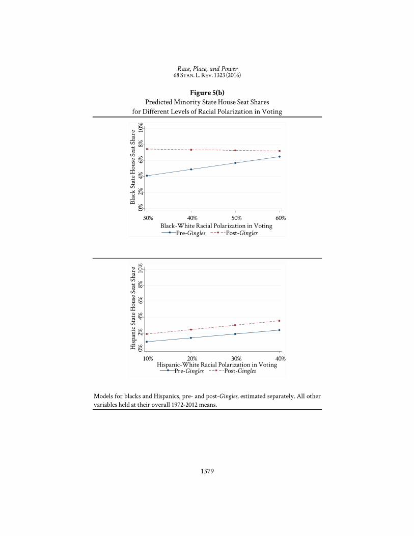
Race, Place, and Power 68 STAN. L. REV. 1323 (2016)
1379
0%
2%
4%
6%
8%
10%
Blac
k St
ate H
ouse
Sea
t Sha
re
30% 40% 50% 60% Black-White Racial Polarization in Voting
Pre-Gingles Post-Gingles
0%
2%
4%
6%
8%
10%
Hisp
anic
Sta
te H
ouse
Sea
t Sha
re
10% 20% 30% 40% Hispanic-White Racial Polarization in Voting
Pre-Gingles Post-Gingles
Figure 5(b) Predicted Minority State House Seat Shares
for Different Levels of Racial Polarization in Voting
Models for blacks and Hispanics, pre- and post-Gingles, estimated separately. All other variables held at their overall 1972-2012 means.

Race, Place, and Power 68 STAN. L. REV. 1323 (2016)
1380
0%
2%
4%
6%
8%
10%
Blac
k St
ate H
ouse
Sea
t Sha
re
1992 1996 2000 2004 2008 2012
No Desegregation Actual Desegregation
Figure 5(c) Actual Share of State House Seats Held by Black Legislators from 1992 to 2012, Versus Predicted Share if Black-White Segregation Had Remained Constant at
Its 1992 Level
Predicted values generated using post-Gingles model for black descriptive representation.
V. Substantive Representation
To some readers, the analysis to this point may have the feel of Hamlet without the prince. The missing prince, of course, is minorities’ substantive representation: the extent to which legislatures, as bodies, promote minorities’ policy interests—and the topic of this Part.276 The literature has typically treated the share of legislative seats held by Democrats or the liberalism of the median legislator as a proxy for substantive representation, and I follow its lead here. The literature has also documented a clear tradeoff between descriptive and substantive representation, arising as adjoining districts are stripped of minority voters in order to create majority-minority districts in which these voters can elect their preferred candidates. However, a handful of
276. See King-Meadows & Schaller, supra note 216, at 168 (“[T]he descriptive-substantive tradeoff remains the central dispute for contemporary scholars of minority representation.”).

Race, Place, and Power 68 STAN. L. REV. 1323 (2016)
1381
non-empirical studies have claimed that this tradeoff can be avoided through savvy line-drawing.
To grasp the relationship between descriptive and substantive representation, I join my dataset of black and Hispanic state house seat shares with three additional datasets: Democratic state house seat shares from 1972 to 2014, median state house member ideologies from 1986 to 2012, and information on which party (if any) was responsible for redistricting in each state during the last five cycles. I find a substantial tradeoff between the election of more minority legislators and the election of more Democrats. This tradeoff, though, is almost eliminated by Democratic control of redistricting but further exacerbated by Republican control. I also find a weaker link between minority seat share and the liberalism of the median legislator. There is again a descriptive-substantive tradeoff, and it is again allayed when Democrats run redistricting but intensified when Republicans are in charge. These effects, though, are comparatively muted.
A. Hypotheses
Substantive representation was a major part of vote dilution law prior to Gingles. The Supreme Court considered the responsiveness of governmental institutions to minority voters’ interests an “important element,”277 and scholars deemed it the “linchpin of pre-1982 constitutional dilution challenges.”278 Gingles, it is true, demoted “evidence demonstrating that elected officials are unresponsive to the particularized needs of the members of the minority group” to secondary status—a mere factor in the totality-of-circumstances inquiry rather than one of the case’s iconic prongs.279 But substantive representation remains doctrinally relevant to this day, and according to many scholars, it deserves more attention than it has received since Gingles. As Pildes has written, “any overall policy assessment of the VRA . . . must explore whether and to what extent the Act promotes the substantive interests of the minority voters it purports to protect.”280
The ideal measure of substantive representation would track how closely legislative outputs track minorities’ distinctive policy preferences. At the
277. Rogers v. Lodge, 458 U.S. 613, 625 n.9 (1982); see also supra notes 49-50 and accompanying text.
278. Guinier, supra note 58, at 1095; see also Issacharoff, supra note 8, at 1868 (“In the case law prior to the 1982 amendments . . . ‘nonresponsiveness’ of elected bodies to the needs and interests of the minority community was a central focus of litigation.”).
279. Thornburg v. Gingles, 478 U.S. 30, 45 (1986). 280. Richard H. Pildes, The Politics of Race, 108 HARV. L. REV. 1359, 1376 (1995) (book review);
see also, e.g., Guinier, supra note 58, at 1091 (arguing that the Act’s “original goals” included “broad-based voter participation, reform, and authentic representation”); Karlan, supra note 81, at 196 (referring to “Congress’ strong desire to reinfuse the [Act] with minority access and civic inclusion”).

Race, Place, and Power 68 STAN. L. REV. 1323 (2016)
1382
congressional level, Cameron and his coauthors281 and Christian Grose282 have used the scores assigned to House members by the Leadership Conference on Civil Rights (LCCR), on the assumption that minority voters feel especially strongly about civil rights issues. At the state legislative level, similarly, Epstein and O’Halloran have calculated how often all members vote consistently with a majority of black members, on the assumption that the latter’s records accurately reflect black voters’ preferences.283 However, LCCR scores have been criticized for counting bills that are “not of central importance to the African-American community,”284 and are unavailable anyway at the state legislative level. Likewise, Epstein and O’Halloran have analyzed only two chambers (over five sessions),285 and their method is not easily generalizable to many states over many years.
Because of these difficulties, the vast majority of scholars studying substantive representation have assessed it using one of two metrics: the share of legislative seats held by Democrats, or the liberalism of the median legislator, determined on the basis of roll call votes. The same logic underpins both of these approaches. Minority voters are (correctly) assumed to lean Democratic and liberal,286 and so to prefer the election of Democratic candidates and the passage of liberal bills. Not all minorities hold these partisan and ideological views, of course, but enough are thought to for the proxies to be valid. Among the academics who have relied on Democratic seat shares are David Canon,287 Grofman and Handley,288 Kevin Hill,289 and Lublin.290 And
281. See Cameron et al., supra note 162, at 799. 282. See GROSE, supra note 103, at 64 (using relevant votes to create a civil rights issue space);
see also Sophie Schuit & Jon C. Rogowski, Race, Representation, and the Voting Rights Act 9 (Nov. 13, 2014) (unpublished manuscript), https://pages.wustl.edu/files/pages /imce/rogowski/vra_and_representation_11_13_2014.pdf (calculating how often House members voted to broaden civil rights).
283. See David L. Epstein & Sharyn O’Halloran, Does the New VRA Section 5 Overrule Georgia v. Ashcroft?, 63 N.Y.U. ANN. SURV. AM. L. 631, 656 (2008) (analyzing the Georgia Senate from 1999 to 2002); Epstein & O’Halloran, supra note 184, at 387-88 (analyzing the South Carolina Senate from 1990 to 1994).
284. DAVID T. CANON, RACE, REDISTRICTING, AND REPRESENTATION: THE UNINTENDED CONSEQUENCES OF BLACK MAJORITY DISTRICTS 175 (1999); see also JOHN D. GRIFFIN & BRIAN NEWMAN, MINORITY REPORT: EVALUATING POLITICAL EQUALITY IN AMERICA 200 (2008) (noting that only about a dozen votes, out of close to a thousand, contributed to LCCR scores in one representative year).
285. See supra note 282. 286. See, e.g., LUBLIN, supra note 213, at 73 (“Black public opinion . . . is . . . quite cohesive and
substantially more liberal than white opinion.”); Norrander & Manzano, supra note 97, at app. tbls.b, c & d (providing tables of average black, Latino, and Asian American ideologies by state).
287. See CANON, supra note 283, at 74.

Race, Place, and Power 68 STAN. L. REV. 1323 (2016)
1383
among the ones who have taken advantage of legislator liberalism derived from roll call votes are Grose (in other work),291 Lublin,292 Lublin and Stephen Voss,293 and Marvin Overby and Kenneth Cosgrove.294
This empirical literature concludes almost unanimously that a tradeoff exists between descriptive and substantive representation. In Cox and Richard Holden’s words, there is a “rough consensus” that “drawing districts that contain a majority of minority voters . . . helps minority voters in those districts but hurts [their preferred party] more broadly.”295 As to Democratic seat share, several studies find that Democrats lost around ten House seats in the 1990s due to the creation of additional majority-minority districts.296 Lublin and Voss arrive at similar estimates at the state legislative level, determining that Democrats lost from two to sixteen seats in each of ten southern state houses from 1991 to 1998 due to the rise in minorities’ descriptive representation.297 As to the median legislator’s ideology too, Cameron and his coauthors,298 Grose,299 and Lublin and Voss300 show that it
288. See Bernard Grofman & Lisa Handley, Estimating the Impact of Voting-Rights-Related Districting on Democratic Strength in the U.S. House of Representatives, in RACE AND REDISTRICTING IN THE 1990S, at 51, 53 (Bernard Grofman ed., 1998).
289. See Kevin A. Hill, Does the Creation of Majority Black Districts Aid Republicans? 1: An Analysis of the 1992 Congressional Elections in Eight Southern States, 57 J. POL. 384, 398 (1995).
290. See LUBLIN, supra note 213, at 111. 291. See Christian R. Grose, Disentangling Constituency and Legislator Effects in Legislative
Representation1: Black Legislators or Black Districts?, 86 SOC. SCI. Q. 427, 438 (2005). 292. See LUBLIN, supra note 213, at 115. 293. See David Lublin & D. Stephen Voss, The Missing Middle1: Why Median-Voter Theory
Can’t Save Democrats from Singing the Boll-Weevil Blues, 65 J. POL. 227, 231, 235 (2003). 294. See L. Marvin Overby & Kenneth M. Cosgrove, Unintended Consequences? 1: Racial
Redistricting and the Representation of Minority Interests, 58 J. POL. 540, 542 (1996). 295. Adam B. Cox & Richard T. Holden, Reconsidering Racial and Partisan Gerrymandering,
78 U. CHI. L. REV. 553, 555 (2011). 296. See CANON, supra note 283, at 74, 257 (summarizing these studies); LUBLIN, supra
note 213, at 111-14 (same). But see Ebonya Washington, Do Majority-Black Districts Limit Blacks’ Representation? The Case of the 1990 Redistricting, 55 J.L. & ECON. 251, 267 tbl.3, 268 (2012) (finding no statistically significant drop in Democratic seat share due to coverage by section 5 of the VRA in the 1990s).
297. See Lublin & Voss, supra note 33, at 802 tbl.2. 298. See Cameron et al., supra note 162, at 808 (showing that allocation of black voters that
maximizes descriptive representation does not maximize substantive representation). 299. See GROSE, supra note 103, at 66, 67 tbl.3.2 (analyzing the U.S. House as a whole and
concluding that the rightward shift of its median was noticeable, if relatively small). 300. See Lublin & Voss, supra note 292, at 231, 233. But see Carlos A. Sanchez-Martinez &
Kenneth W. Shotts, Assessing Robustness of Findings About Racial Redistricting’s Effect on Southern House Delegations, 6 STAT. POL. & POL’Y 97, 100-12 (2015) (finding no statistically significant relationship between the share of majority-minority districts
footnote continued on next page

Race, Place, and Power 68 STAN. L. REV. 1323 (2016)
1384
became more conservative in the 1990s in House delegations that gained minority members. Likewise, according to Epstein and O’Halloran, the midpoint of the South Carolina Senate shifted to the right after its map was redrawn in 1992 with more majority-minority districts.301
A simple dynamic likely accounts for these findings. Minority voters tilt Democratic and liberal302 and also tend to be polarized from white voters.303 Because of this polarization, districts with large shares (usually majorities) of minority voters need to be created to assure them the ability to elect their preferred candidates. But these voters need to be removed from adjacent districts, which become whiter as a result of the minorities’ removal. And by becoming whiter, the neighboring districts grow more Republican and conservative as well. A tradeoff thus emerges between descriptive and substantive representation. Enabling the election of minorities’ candidates of choice in certain districts requires making other districts more likely to elect minorities’ least-preferred candidates: conservative Republicans.304
But a few observers—in particular, Cox and Holden305 and Kenneth Shotts306—dispute this account, albeit non-empirically. They point out that majority-minority districts need not be drawn in a manner that over-concentrates minority voters and wastes Democratic votes. Instead, they can be designed with bare majorities (or even pluralities) of minority voters, combined with large minorities of conservative white voters. This strategy relaxes the descriptive-substantive tradeoff by making districts in which
and the share of southern states’ House members with ideologies to the left of the overall House median over the 1986-1996 period); Joseph Simons & Daniel J. Mallinson, Party Control and Perverse Effects in Majority-Minority Districting1: Replication Challenges When Using DW-NOMINATE, 6 STAT. POL. & POL’Y 19, 30-34, 31 tbl.3 (2015) (same over the 1988-2008 period); Washington, supra note 295, at 267 tbl.3, 268 (finding no statistically significant rightward shift in average House member ideology due to coverage by section 5 in the 1990s).
301. See Epstein & O’Halloran, supra note 184, at 392 tbl.5. 302. See supra note 285 and accompanying text. 303. See supra Part II.B. 304. See Cox & Holden, supra note 294, at 557-62 (summarizing the “pack-and-crack
consensus” as to this dynamic (capitalization altered)). 305. See id. at 573 (explaining that the optimal Democratic strategy is to create majority-
minority districts “with the thinnest margin[s] between Democrats and Republicans”). 306. See Kenneth W. Shotts, The Effect of Majority-Minority Mandates on Partisan
Gerrymandering, 45 AM. J. POL. SCI. 120, 121 (2001) (predicting based on a formal model that “where Democrats control redistricting,” the descriptive-substantive tradeoff may not apply “because gerrymanderers can draw majority-minority districts with no excess Democratic votes”); see also Kenneth W. Shotts, Does Racial Redistricting Cause Conservative Policy Outcomes? 1: Policy Preferences of Southern Representatives in the 1980s and 1990s, 65 J. POL. 216, 221-22, 221 tbl.1 (2003) (finding that unified Democratic control over redistricting increased the share of southern states’ House members with ideologies to the left of the overall House median over the 1988-1996 period).

Race, Place, and Power 68 STAN. L. REV. 1323 (2016)
1385
minorities elect their preferred candidates no safer for Democrats than a plan’s other districts. Only a Democratic line-drawer, though, is likely to adopt this approach. A Republican line-drawer is likely to prefer packing minorities (and other reliable Democrats) into a handful of districts that they win by overwhelming margins. Republican candidates then enjoy an advantage in all of a plan’s remaining districts.307
Based on the empirical literature, it is reasonable to expect descriptive and substantive representation to be negatively related at the state house level over the modern redistricting era. This literature has focused on Congress in the 1990s, but its findings seem applicable to other chambers and periods. And based on the nonempirical studies, it is reasonable to expect the severity of the descriptive-substantive tradeoff to vary based on the party that is responsible for redistricting. The tradeoff is likely steepest when Republicans have unified control of the process, mildest when Democrats are fully in charge, and somewhere in between when neither party has sole authority.308
To these predictions I would add one more, derived from the extensive work showing that legislators tend to be ideologically close to their copartisans and far from the opposing party’s members, in both Congress and state legislatures.309 This hypothesis is that the descriptive-substantive tradeoff should be more pronounced with respect to Democratic seat share, and less stark with respect to median legislator ideology. In the former case, legislative polarization seems irrelevant, but in the latter, it suggests that chambers’ midpoints should not change much unless additional majority-minority districts actually cause chambers to flip from blue to red. Without a switch in party control, in a polarized environment, the legislative median should be relatively insensitive to fluctuations in party seat share.310
307. See Cox & Holden, supra note 294, at 588 (clarifying that this is the “second-best strategy” for Republicans, undertaken only when the VRA compels them to create majority-minority districts).
308. It is also possible that the relationship between descriptive and substantive representation varies by region or period. For example, the tradeoff between them might be more severe in the South, where white voters tend to be more conservative than in the non-South. The tradeoff might also be more severe in recent years, since the Supreme Court has rendered unavailable certain policies (like bizarrely shaped majority-minority districts) that make it easier to achieve descriptive and substantive representation simultaneously. These are fruitful topics for further study.
309. See, e.g., The Polarization of the Congressional Parties, VOTEVIEW, http://voteview.com /political_polarization_2014.htm (last updated Mar. 21, 2015) [hereinafter Congressional Polarization] (showing congressional polarization from 1879 to 2014); Shor & McCarty, supra note 31, at 540 fig.7 (showing state legislative polarization over last two decades).
310. Cf. GROSE, supra note 103, at 55 (“Party control of the legislature is . . . what matters for promoting civil rights outcomes, and racial redistricting has had only a small impact on party control.”).

Race, Place, and Power 68 STAN. L. REV. 1323 (2016)
1386
B. Trends
Before testing these hypotheses, I describe the trends in Democratic seat share and median legislator ideology, in both the South and the non-South, over all available years. I compiled Democratic seat shares in state houses from 1972 to 2012 as part of an earlier project.311 In a breakthrough study, Boris Shor and Nolan McCarty also estimated state legislator ideologies from 1986 to 2012 using state legislative roll call votes.312 These ideologies range from about -1 (very liberal) to about 1 (very conservative);313 they are analogous to the NOMINATE scores that scholars have relied on for decades to study the positions of members of Congress;314 and they have never before been used to analyze minorities’ substantive representation.
As shown in Figure 6’s first chart, the Democratic seat share in the average southern state house has declined steadily over the last four decades. It neared 90% in the mid-1970s, crossed the 50% threshold around 2000, and fell to roughly 35% after the 2014 election. In contrast, the Democratic seat share in the average nonsouthern state house has held relatively steady over this period, though it too dipped from about 60% in the 1970s and 1980s to about 50% in the 1990s, 2000s, and 2010s. In recent years, the strong Democratic showings in the 2006 and 2008 elections are evident, as are the Republican waves of 2010 and 2014.
Figure 6’s second chart displays the changes in the ideology of the median member of the average southern and the average nonsouthern state house. In the South, the chamber midpoint grew ever more conservative from 1986 to 2012, from near -0.2 to above 0.7 (on the -1 to 1 scale). The most dramatic spikes in the median member’s conservatism took place after the 2002 and 2010 elections, when several chambers flipped from Democratic to Republican control. In the non-South, on the other hand, the ideological trajectory was much flatter over this period, hovering around 0, though it too reveals a gradual increase in the median member’s conservatism. Again, a clear leftward shift is apparent after the 2006 and 2008 elections, as well as an even more striking swing to the right after 2010.
311. See Stephanopoulos & McGhee, supra note 30, at 868-69; see also Jackman Report, supra note 30, at 19-21.
312. See Shor & McCarty, supra note 31, at 532-43; Shor & McCarty Data, supra note 31 (expanding time coverage of original study).
313. See Shor & McCarty, supra note 31, at 539 fig.6. 314. See Congressional Polarization, supra note 308.

Race, Place, and Power 68 STAN. L. REV. 1323 (2016)
1387
30%
40%
50%
60%
70%
80%
90%
Dem
ocra
tic S
tate
Hou
se S
eat S
hare
1970 1980 1990 2000 2010
Non-South South
Figure 6(a)
Trends in the Share of State House Seats Held by Democrats, in the Average State, by Election Year
Values calculated separately for states in the South and the non-South. The vertical dotted line indicates the 1986 Gingles decision.

Race, Place, and Power 68 STAN. L. REV. 1323 (2016)
1388
-.2
0 .2
.4 .6
.8 St
ate H
ouse
Med
ian
NPA
T
1986 1990 1994 1998 2002 2006 2010
Non-South South
Figure 6(b) Trends in the Ideology of the Median State House Member, in the Average
State, by Election Year
Values calculated separately for states in the South and the non-South.
C. Drivers
Turning from the trends in substantive representation to its relationship with descriptive representation, I constructed a pair of models with Democratic seat share and median member ideology, respectively, as the dependent variables. The key independent variables were the combined black and Hispanic seat share in each state, interacted with dummy variables for unified Democratic and Republican control over redistricting.315 I used the combined minority seat share, instead of each group’s separate proportion, to avoid the proliferation of interaction terms.316 I also used the interactions themselves to allow the link between substantive and descriptive
315. The omitted category is the enactment of a district plan by anything other than unified Democratic or Republican government.
316. For another recent analysis combining blacks and Hispanics for similar reasons, see Ansolabehere et al., supra note 167, at 1413-20.

Race, Place, and Power 68 STAN. L. REV. 1323 (2016)
1389
representation to vary based on party control.317 And I determined which institution was responsible for designing each state’s district plan in each cycle in previous work.318 Unified party control means a party held both the governorship and majorities in each legislative chamber. Nonunified control means a plan was enacted by a divided government, a court, or a redistricting commission.
The most important control in the models is the Democratic share of the statewide vote. A party’s popular support, of course, is a powerful driver of both the share of seats the party wins and the ideology of the pivotal legislator. I also calculated Democratic vote shares in previous work, using presidential election results to impute the outcomes of state house races that were uncontested.319 The combined black and Hispanic population share is included as a control as well, in case it influences substantive representation directly, and not only through its impact on the combined minority seat share.320 And as in this Article’s other models, I add fixed effects for years and states too, thus taking into account time trends and time-invariant differences among states.321
Figure 7’s first chart shows the relationship between the share of Democrats and the share of minority legislators elected, varying the institution in charge of redistricting and holding all other variables at their means. When neither party has unified line-drawing control, this relationship is negative and statistically significant.322 For instance, an increase in the minority seat share from 0% to 25% (or roughly its tenth to its ninetieth percentile) results in a decline in the Democratic seat share from about 57% to about 52%. When Democrats are fully responsible, however, the slope of this relationship remains almost the same, but its intercept rises by a statistically significant margin of
317. See Simons & Mallinson, supra note 299, at 20 (“[I]t seems likely that the ideological effect of majority-minority districting interacts with the party in control of the state legislature.”).
318. See Nicholas O. Stephanopoulos, Arizona and Anti-Reform, 2015 U. CHI. LEGAL F. 477, 497-99.
319. See Stephanopoulos & McGhee, supra note 30, at 865-67; see also Jackman Report, supra note 30, at 22-32.
320. See Simons & Mallinson, supra note 299, at 28 (“[W]e also choose to include variables measuring the percentage of the state’s population that is Black and Hispanic, respectively.”).
321. However, I did not construct separate pre- and post-Gingles models because there is insufficient legislator ideology data for the pre-Gingles period. In addition, Gingles1’s most important effect, the increase in minorities’ descriptive representation, is already captured in the models’ key independent variable, combined minority seat share. There is no reason to expect Gingles to have changed the relationship between descriptive and substantive representation.
322. See infra Appendix Table 3.
Race, Place, and Power 68 STAN. L. REV. 1323 (2016)
1390
roughly 3 percentage points.323 That is, Democrats win about 60% of seats when the minority seat share is 0%, and about 55% of seats when the minority seat share is 25%. And when Republicans have sole authority, the slope of the predicted value curve steepens significantly.324 In this scenario, Democrats win close to 57% of seats when the minority seat share is 0%, but only 47% of seats when the minority seat share is 25%.
These results are highly consistent with expectations. As predicted based on the literature focusing on Congress in the 1990s,325 there is indeed a tradeoff between electing minority legislators and electing Democrats to state houses over the 1972-2014 period. As more districts are created in which minority voters are able to elect their preferred candidates, adjacent districts evidently become less diverse and more Republican, leading to the victory of fewer Democrats overall. As also predicted based on the non-empirical studies,326 this tradeoff varies based on the party that is responsible for redistricting. The tradeoff is alleviated by Democratic line-drawers (who seek to avoid over-concentrating minority voters), but exacerbated by Republican line-drawers (who aim to pack them). This is perhaps an intuitive outcome, but it has not previously been demonstrated with real-world evidence.
Next, Figure 7’s second chart displays the relationship between the ideology of the median state house member and the proportion of minority legislators elected, again varying the institution in charge of redistricting and holding all other variables at their means. When neither party has unified line-drawing control, there is a positive link between the median member’s conservatism and the minority seat share. However, this link is neither statistically significant nor substantively large, amounting to only a 0.15 swing to the right (on the -1 to 1 scale) as the minority seat share increases from 0% to 25%.327 When Democrats are fully responsible, the slope of the predicted value curve flattens and its intercept shifts by about 0.1 in a liberal direction. These effects, though, are not statistically significant either.328 And when Republicans have sole authority, the curve’s slope steepens, producing a rightward move of roughly 0.3 in the median member’s ideology as the minority seat share rises from 0% to 25%. But these effects too do not rise to statistical significance.329
323. See id. 324. See id. 325. See supra note 295 and accompanying text. 326. See supra notes 304-06 and accompanying text. 327. See infra Appendix Table 3; see also GROSE, supra note 103, at 66 (describing a “range of -
0.2 and 0.2” as “narrow and moderate”). 328. See infra Appendix Table 3. 329. See id.

Race, Place, and Power 68 STAN. L. REV. 1323 (2016)
1391
These findings also conform nicely to expectations. There is again a descriptive-substantive tradeoff, and it is again eased by unified Democratic control but aggravated by unified Republican control. And as expected based on the literature on legislative polarization,330 this tradeoff is less severe—never becoming statistically significant—than the one between the share of Democrats and the share of minority legislators elected. This looser connection likely stems from the fact that each party’s members tend to be both ideologically cohesive and ideologically distant from the opposing party’s members.331 Accordingly, shifts in seat share caused by the creation of additional majority-minority districts typically have little impact on the position of the median member. The seat share shifts only move the chamber’s midpoint much on the rare occasions when they bring about a switch in party control.
To ensure the reliability of these results, I subject them to a final barrage of robustness checks. I replace the state fixed effects with state random effects; I consider only observations postdating Gingles, in case the descriptive-substantive tradeoff was influenced by the decision; and I drop the interactions between minority seat share and unified Democratic and Republican control. None of these checks materially alters my conclusions. In the Democratic seat share models, minority seat share retains its significant negative coefficient in all but one case (the post-Gingles model), unified Democratic control keeps its significant positive coefficient in all cases, and the interaction between minority seat share and unified Republican control stays significantly negative in all but one case (also the post-Gingles model).332 Likewise, in the median member ideology models, all of the relevant variables continue not to rise to statistical significance in all but one case (a significant negative coefficient for unified Democratic control in the model without interactions).333
We can therefore be reasonably sure that the contours of the relationship between substantive and descriptive representation, as presented here, are accurate. These contours’ main features, again, are a distinct tradeoff between Democratic and minority seat share and a weaker link between the median member’s ideology and the proportion of minority legislators elected. And as to both Democratic seat share and the chamber’s ideological midpoint, a greater substantive sacrifice is needed to improve descriptive representation when Republicans are responsible for redistricting—but almost no sacrifice at all when Democrats are in charge.
330. See supra note 308 and accompanying text. 331. See id. 332. See infra Appendix Table 3. If anything, this suggests that the tradeoff between
Democratic and minority seat share has weakened since Gingles, even under unified Republican control of redistricting.
333. See id.

Race, Place, and Power 68 STAN. L. REV. 1323 (2016)
1392
45%
50%
55%
60%
65%
Dem
ocra
tic S
tate
Hou
se S
eat S
hare
0% 5% 10% 15% 20% 25% Minority State House Seat Share
Non-Unified Control Unified Democratic Control Unified Republican Control
Figure 7(a)
Predicted Democratic State House Seat Shares for Different Minority State House Seat Shares
Predictions shown separately for scenarios of nonunified control over redistricting, unified Democratic control, and unified Republican control. All other variables held at their means.

Race, Place, and Power 68 STAN. L. REV. 1323 (2016)
1393
-.2
-.1
0 .1
.2 St
ate H
ouse
Med
ian
NPA
T
0% 5% 10% 15% 20% 25% Minority State House Seat Share
Non-Unified Control Unified Democratic Control Unified Republican Control
Figure 7(b) Predicted Ideology of Median State House Member for Different Minority
State House Seat Shares
Predictions shown separately for scenarios of nonunified control over redistricting, unified Democratic control, and unified Republican control. All other variables held at their means.
VI. Implications
Where, then, does all of this empirical analysis leave us? On balance, given the findings of the four preceding parts, would we say that Gingles has been a success or a failure? And are there ways in which this Article’s investigation could be extended in future work, thus deepening our understanding of race and representation in contemporary America? In this Part, I take up these questions. I first present the positive case for Gingles1’s impact. Thanks to the decision, blacks’ descriptive representation improved dramatically, and in precisely the circumstances of racial segregation and polarization contemplated by the Court. The share of black legislators also surged without imposing an inordinate substantive cost.
Next, I go through the snags in the story. Minority voters have been no less polarized since Gingles than they were beforehand. The decision has not produced the same descriptive gains for segregated and polarized Hispanic populations that it has for black ones. And the descriptive-substantive tradeoff is fairly steep in today’s most common political environment (namely, unified

Race, Place, and Power 68 STAN. L. REV. 1323 (2016)
1394
Republican control over redistricting). Lastly, I identify some promising avenues for future research. All of the elements of the Gingles framework could be examined using local (rather than state-level) data. The natural experiment set into motion by Gingles could be exploited in additional ways. And information about where minorities are underrepresented, given their geographic distribution and voting patterns, could generate a new coverage formula to replace the one recently nullified by the Court.
A. Positive
The first entry on the positive side of the Gingles ledger is the striking decline in black-white segregation over the last four decades. The spatial index of dissimilarity for blacks and whites stood at almost 70% in the average state in 1970, but fell to below 50% by 2010 (and below 40% in the average southern state).334 This trend means that blacks are considerably more residentially integrated (and less geographically compact) today than they were in the relatively recent past.
However, it is probably incorrect to call this development a feather in Gingles1’s cap. The presence of geographic compactness may be one of the decision’s preconditions for liability, but its reduction has never been understood to be one of the case’s goals. Neither Gingles itself, nor any other pronouncement by the Court about section 2, nor the provision’s text or legislative history, articulates a desegregative aspiration.335 Other federal statutes do so, like the Fair Housing Act336 and the Community Reinvestment Act,337 but this is not the province of the Voting Rights Act. Accordingly, the rise in black-white integration seems mostly irrelevant to any assessment of Gingles1’s record.
Far more germane, though, is the rise in black descriptive representation since the decision. The Gingles Court declared that minority voters’ inability “to elect their preferred representatives” is the “essence of a § 2 claim,”338 and most section 2 plaintiffs have concurred in “[t]he belief that black
334. See supra Part II.B. However, Hispanic-white spatial segregation stayed constant at close to 40% over this period. See id.
335. See Stephanopoulos, supra note 17 (manuscript at 45) (“Integration is not one of Section 2’s goals. But minority representation is one of them, and . . . is imperiled by desegregation.”).
336. See Tex. Dep’t of Hous. & Cmty. Affairs v. Inclusive Cmties. Project, Inc., 135 S. Ct. 2507, 2525-26 (2015) (noting “the Fair Housing Act’s continuing role in moving the Nation toward a more integrated society”).
337. See 12 U.S.C. § 2903(a)(1) (2014) (providing that financial institutions be evaluated based on their “record[s] of meeting the credit needs of [their] entire communit[ies], including low- and moderate-income neighborhoods”).
338. Thornburg v. Gingles, 478 U.S. 30, 47 (1986).

Race, Place, and Power 68 STAN. L. REV. 1323 (2016)
1395
representation is everything.”339 This belief has become reality in the post-Gingles era. In the average southern state, the share of black state house members has jumped from about 13% before the decision to roughly 20% today.340 In the average nonsouthern state with a sizeable black population, this proportion has grown from around 9% to close to 14%.341 And in both the South and the non-South, the black population share and the black seat share are now closely correlated, while prior to Gingles they exhibited only a weak relationship.342
Even more importantly, this improvement has come about via the very mechanism devised by the Court. Gingles famously converted racial segregation and polarization from mere aspects of the totality-of-circumstances inquiry into prerequisites for liability.343 Consistent with the Court’s design, segregated and polarized black populations have made impressive progress since the decision in their ability to elect their preferred candidates. In the average state in the post-Gingles period, the predicted black seat share is anywhere from 0.5 to 3 percentage points higher at any level of segregation than it was in the pre-Gingles era.344 Likewise, the predicted black seat share is anywhere from 0.5 to 3.5 percentage points higher at any level of polarization.345 These figures represent an increase in black descriptive representation of up to 80%—and thus a compelling rejoinder to the pessimistic thesis that courts cannot produce meaningful social change.346
Furthermore, the worry that such change could be achieved only by undermining black substantive representation turns out to be overblown. In the average state, the combined minority seat share grew from 6% before Gingles to 11% afterward.347 When neither party has unified control over redistricting, a rise in descriptive representation of this magnitude leads to a fall in the Democratic seat share of only 1 percentage point (56% to 55%) and an increase in the median state house member’s conservatism of only 0.03 (-0.02 to 0.01).348
339. Guinier, supra note 58, at 1078. 340. See supra Part IV.B. 341. See id. These figures are for nonsouthern states with black populations of at least 10%. 342. See id. Specifically, the correlation is 0.87 in the South and 0.60 in the non-South in the
post-Gingles period, compared to 0.30 and 0.12, respectively, in the pre-Gingles era (again only including states with black populations of at least 10%).
343. See supra Part I.A. 344. See supra Part IV.C. 345. See id. 346. See generally MICHAEL J. KLARMAN, FROM JIM CROW TO CIVIL RIGHTS: THE SUPREME
COURT AND THE STRUGGLE FOR RACIAL EQUALITY (2004); GERALD N. ROSENBERG, THE HOLLOW HOPE: CAN COURTS BRING ABOUT SOCIAL CHANGE? (2d ed. 2008).
347. See supra Part IV.B. 348. See supra Part V.C.

Race, Place, and Power 68 STAN. L. REV. 1323 (2016)
1396
When Democrats are responsible for redistricting, the descriptive-substantive tradeoff is equally small—and dwarfed by a 3 percentage point boost in the Democratic seat share and a leftward shift of 0.10 in the chamber’s midpoint.349 Accordingly, even if Gingles must be judged based on how well it “promotes the substantive interests of the minority voters it purports to protect,”350 the verdict is positive. Under many political environments,351 minorities pay either a low substantive price, or no price at all, for better descriptive representation.
In my view, these positive points ultimately carry the day. Gingles1’s primary objective was to enable geographically and politically distinct groups of black voters to elect their preferred candidates. The decision has done exactly that, and without requiring a significant substantive sacrifice in the process. But to this optimistic account several notable caveats must be appended, which I next discuss.
B. Negative
An initial caveat is that Gingles has not accomplished its secondary goal of inducing “white voters [to] join[] forces with minority voters to elect their preferred candidate[s].”352 In the typical nonsouthern state, black-white polarization did not fall at all following the decision. It averaged 46% beforehand, and 46% afterward.353 In the typical southern state, black-white polarization actually worsened substantially in the case’s wake, from a pre-Gingles average of 51% to a post-Gingles mean of 63%.354 And while Hispanic-white polarization in the typical state edged downward after the decision, from an average of 29% to a mean of 22%, this mild improvement was erased in the most recent presidential election, when it returned to 29%.355 Minority voters thus remain as electorally isolated as ever—and as reliant on the “second best” solution of majority-minority districts, which alone can ensure descriptive representation under polarized conditions.356
349. See id. 350. Pildes, supra note 279, at 1376. 351. In my database, there are 255 cases of unified Democratic control over redistricting,
146 cases of unified Republican control, and 502 cases in which neither party has full line-drawing authority.
352. Bartlett v. Strickland, 556 U.S. 1, 25 (2009) (plurality opinion). 353. See supra Part III.B. 354. See id. 355. See id. 356. See Johnson v. De Grandy, 512 U.S. 997, 1020 (1994) (commenting that majority-
minority districts “rely on a quintessentially race-conscious calculus aptly described as the ‘politics of second best’” (quoting GROFMAN ET AL., supra note 15, at 136)). And to be more precise, majority-minority districts are the only single-member constituencies
footnote continued on next page

Race, Place, and Power 68 STAN. L. REV. 1323 (2016)
1397
Second, not only is polarization not waning, it is also perversely related to Gingles1’s first prong, at least for blacks. When blacks become more residentially integrated (and so less geographically compact), their voting patterns grow somewhat more different from those of whites.357 Consistent with the threat theory of race relations, more interracial contact leads to greater political divergence. This effect, though, is not particularly large, as the 20 percentage point decline in black-white segregation since 1970 is responsible for only about a 5 percentage point increase in black-white polarization.358 Nor does the effect extend to Hispanics, for whom segregation and polarization are unconnected.359 Still, it is disheartening that Gingles1’s prongs sometimes operate at cross-purposes rather than in harmony.
Third, it is also discouraging that the prongs have not benefited segregated and polarized Hispanic populations to the same extent as black ones. In the average state in the post-Gingles period, the predicted Hispanic seat share is slightly higher at some levels of segregation than in the pre-Gingles era but slightly lower at others.360 Similarly, the predicted Hispanic seat share is only about 1 percentage point higher at any level of polarization.361 These gains in descriptive representation are much smaller and more erratic than those enjoyed by blacks since the decision.362 They suggest that Hispanic votes continue to be diluted in many areas, likely because, in defiance of Gingles, segregated and polarized Hispanic groups often fail to be enclosed within districts of their own. In the future, these groups may be well-positioned to mount section 2 challenges, but to date, their lack of progress is evident.363
Fourth, even Gingles1’s crown jewel, black descriptive representation, is in danger of being tarnished by the decrease in black-white segregation. Already, the proportion of black legislators has grown by about 1 percentage point less over the last two decades than it would have had blacks not integrated over this timeframe.364 Going forward, the black seat share could plausibly start to fall as black voters become too spatially dispersed for districts to be drawn
that can guarantee descriptive representation under polarized conditions. Alternative electoral systems such as cumulative, limited, or preferential voting can also enable polarized groups to elect their preferred candidates.
357. See supra Part III.C. 358. See id. 359. See id. 360. See supra Part IV.C. 361. See id. 362. See id. 363. The findings for Hispanic voters also suggest that remedies other than single-member
districts, such as multimember districts paired with cumulative, limited, or preferential voting, may be needed to provide them with descriptive representation. See Stephanopoulos, supra note 85, at 846-55 (arguing for these alternative remedies).
364. See supra Part IV.C.

Race, Place, and Power 68 STAN. L. REV. 1323 (2016)
1398
around them in certain regions. This outcome has been averted so far thanks to a favorable time trend,365 but there is no guarantee this trend will persist.
Lastly, while it is true enough that there is not necessarily a sharp tradeoff between descriptive and substantive representation, it is equally true that there is sometimes one. Take a state whose combined minority seat share rose from about 10% before Gingles to roughly 25% today (a common enough scenario).366 Assume also that Republicans had unified control over redistricting throughout this period, and that all other variables held constant. Then the predicted proportion of Democrats in the state house would have dropped from around 53% to close to 47%, or enough to flip control of the chamber.367 Analogously, the predicted conservatism of the median legislator would have increased by about 0.20, or roughly 10% of the entire ideological range.368 These are substantial effects, large enough to stoke the fear that greater “descriptive representation might be achievable only at the weighty cost of declining substantive representation.”369
In combination, these qualifications dampen any enthusiasm generated by the earlier positive points. The fact that segregated and polarized Hispanic populations now elect scarcely any more Hispanic legislators than they did prior to Gingles is especially damning. It means that the decision’s core value—enabling geographically and politically distinct groups to elect their preferred candidates—has not been realized for America’s most numerous minority. Still, I think it is fairest to see the Court’s intervention as an incomplete success rather than a thoroughgoing failure. Gingles did enable segregated and polarized black populations to elect many more of their candidates of choice, and usually without undercutting their substantive representation along the way. This accomplishment, it is true, must be weighed against the case’s comparative inefficacy in aiding Hispanic voters. But the latter fault does not negate the former feat.
C. Extensions
Beyond assessing Gingles, it is worth noting here some of the ways in which our grasp of the decision’s impact, and of race and representation generally, could be extended. These suggestions involve new sources of data,
365. See id. 366. See supra Part IV.B (showing trends in descriptive representation). This premise
accurately describes Arizona, Georgia, Illinois, and Maryland, among others. 367. See supra Part V.C. 368. See id. 369. Richard H. Pildes, Principled Limitations on Racial and Partisan Redistricting, 106 YALE
L.J. 2505, 2531 (1997).

Race, Place, and Power 68 STAN. L. REV. 1323 (2016)
1399
new kinds of analysis, and new doctrinal applications. Together, they form an exciting research agenda, and one I hope to pursue in future work.
To begin with, how segregation and polarization are related to descriptive representation, and how descriptive and substantive representation are connected, could be studied at the local (rather than the state or federal) level. More than 70% of section 2 litigation involves policies enacted by local governments (primarily electoral arrangements alleged to be dilutive).370 But to date, the literature has focused on Gingles1’s implications for Congress,371 and even this Article is limited to state legislatures. The local context thus offers the most fertile soil in this academic domain that has yet to be tilled.
Does the data exist for this tilling? I believe so. Segregation at the county or city level can be calculated using readily available information about census tracts’ racial compositions.372 Polarization for counties or cities cannot be determined using state or national exit polls, because these surveys usually do not track respondents’ exact locations. But as Amos and McDonald have demonstrated, local polarization can be computed, in a manner that allows comparisons across jurisdictions and over time, by applying ecological inference techniques to precinct-level presidential election results.373 Furthermore, several scholars have already compiled data on local descriptive representation, in the form of city and county councilmembers’ racial affiliations.374 And while the study of local substantive representation is still in its infancy, Cheryl Boudreau and her coauthors have shown that it can be estimated in the same fashion as congressional and state legislative ideology.375 All of the pieces are therefore in place for a local government version of this Article to be written.
Another worthwhile project would be to measure polarization in a way that eliminates the mismatch between its electoral level and that of descriptive
370. See Cox & Miles, supra note 45, app. 1 at 54; see also Shelby Cty. v. Holder, 679 F.3d 848, 872 (D.C. Cir. 2012), rev’d, 133 S. Ct. 2612 (2013) (pointing out that local practices accounted for more than 90% of preclearance denials under section 5 in recent years).
371. See supra Part I.B. 372. See supra notes 129-32 and accompanying text; see also Residential Segregation, SPATIAL
STRUCTURES SOC. SCIS., BROWN UNIV., http://www.s4.brown.edu/us2010 /segregation2010/Default.aspx (last visited June 6, 2016) (providing segregation scores for cities and metropolitan areas from 1980 to 2010).
373. See Amos & McDonald, supra note 166, at 1 (pointing out that their “precinct point estimates can be aggregated to any geographic level”).
374. See, e.g., Marschall et al., supra note 248, at 113-14; Tim R. Sass & Bobby J. Pittman, Jr., The Changing Impact of Electoral Structure on Black Representation in the South, 1970-1996, 104 PUB. CHOICE 369, 378 (2000); Trounstine & Valdini, supra note 102, at 557.
375. See Cheryl Boudreau et al., Informing Electorates via Election Law1: An Experimental Study of Partisan Endorsements and Nonpartisan Voter Guides in Local Elections, 14 ELECTION L.J. 2, 13-14 (2015) (using roll call votes to estimate San Francisco councilmembers’ ideal points).

Race, Place, and Power 68 STAN. L. REV. 1323 (2016)
1400
representation. (Here, for instance, I calculate polarization using presidential voting patterns, and descriptive representation using state house minority seat shares.376) It does not seem possible to bridge this gap by simply computing polarization for the same elections in which the relevant candidates run for office. While this can be done (and, indeed, is done in most section 2 suits), the resulting estimates cannot be compared cross-sectionally or temporally because they are based on different candidates competing against different opponents.377
One solution, which I employed earlier as a robustness check, is to measure ideological polarization, rather than polarization in voting, using exit poll respondents’ self-professed conservatism, liberalism, or moderation.378 A three-point scale, though, is fairly crude and fails to capture the full range of policy preferences. A more sophisticated approach is therefore to ask respondents about dozens of issues and then to distill their answers into ideal points that capture in a single score their overall ideologies.379 Elmendorf and Spencer have used this method to gauge racial polarization in all U.S. counties,380 and their work could be combined with additional county data to analyze Gingles1’s impact at the county level. The most promising option, though, may be to conduct surveys that present respondents with hypothetical candidates whose key attributes (race, party, ideology, incumbency, and so on) are randomly varied.381 The voting preferences that respondents express would then be both comparable across jurisdictions and over time and applicable to the same electoral level at which descriptive representation is determined.
Still another idea is to further exploit Gingles1’s status as a natural experiment, in which the Court announced a standard for vote dilution cases that was not anticipated by potential plaintiffs and defendants.382 Gingles1’s
376. See supra note 267 and accompanying text. 377. See Elmendorf et al., supra note 8 (manuscript at 80) (noting that “candidate attributes
mediate the relationship between racial polarization in political preferences and polarization in vote shares” and “reflect strategic choices by candidates and other actors”).
378. See supra Part III.B. 379. See, e.g., Chris Tausanovitch & Christopher Warshaw, Measuring Constituent Policy
Preferences in Congress, State Legislatures, and Cities, 75 J. POL. 330, 331-36 (2013) (calculating the average ideal points of respondents in states, congressional and state legislative districts, and cities).
380. See Elmendorf & Spencer, supra note 84, at 2195-216. 381. See generally Marisa A. Abrajano et al., Using Experiments to Estimate Racially Polarized
Voting (UC Davis Legal Studies Research Paper Series, Research Paper No. 419, 2015). 382. See Conor M. Dowling et al., Does Public Financing Chill Political Speech? 1: Exploiting a
Court Injunction as a Natural Experiment, 11 ELECTION L.J. 302, 307 (2012) (observing that when courts make decisions, “they often unintentionally act as social experimenters, giving researchers the opportunity to examine the effects of the law in a way that
footnote continued on next page

Race, Place, and Power 68 STAN. L. REV. 1323 (2016)
1401
surprise intervention underpinned my earlier comparison of the relationships between segregation and polarization on the one hand, and descriptive representation on the other, before and after the decision.383 Because Gingles was so unexpected, any changes in the relationships could reasonably be attributed to it rather than to unrelated time trends.384
However, my analysis included all states for the sake of thoroughness and did not distinguish between states that were more or less likely to be affected by the case. Future work could try to divide states into two categories: those for which Gingles was binding (because they had substantial minority populations and relatively few majority-minority districts) and those for which the decision did not act as a constraint (because they had small minority populations or sufficient majority-minority districts).385 The question would then be whether the first group of states was influenced by the decision in a different way than the second one—in terms of the levels of descriptive and substantive representation, how segregation and polarization relate to the former, and how the former is linked to the latter. If so, that would be even stronger evidence of Gingles1’s impact.
Finally, it might be possible to use variants of this Article’s regression models to develop a new coverage formula for the Voting Rights Act. The Act’s formula determines which jurisdictions are subject to section 5’s preclearance requirement, and so must win the approval of the Department of Justice or a
makes clear causal inferences”). Relatedly, the Court’s racial gerrymandering decisions in the 1990s, which also were not anticipated by potential plaintiffs and defendants, could be treated as a natural experiment as well. But because it becomes difficult to employ my modeling strategy (especially the year and state fixed effects) when the data is broken down by decade, a different approach may be necessary to determine these cases’ impact.
383. See supra Part IV.C. 384. More precisely, the differences between the pre-Gingles and post-Gingles periods
represent an upper bound for the magnitude of the decision’s impact. If there were unrelated time trends, they could account for a portion of the impact attributed here to the Court’s intervention.
385. See Washington, supra note 295, at 255-58 (employing a similar methodological strategy but considering all states covered by section 5 to be affected by Gingles and all uncovered states to be unaffected). A potential problem with this difference-in-differences design is that all states may have been affected by Gingles, at least at the state legislative level, since minority seat share universally lagged minority population share prior to the decision. See supra Part IV.B. This problem, though, might be addressable by dividing states into other pairs of categories, such as low versus high segregation or low versus high polarization. These pairings would enable the testing of the hypothesis that Gingles had a greater impact in states with high segregation and high polarization, where its prongs were presumably easier to satisfy. But even this approach would not be methodologically clean, since Gingles did apply to low-segregation and low-polarization states. In the end, there may not be a satisfactory treatment group and control group, given the decision’s consequences throughout the country.

Race, Place, and Power 68 STAN. L. REV. 1323 (2016)
1402
federal court before changing any of their election laws.386 In the 2013 case of Shelby County v. Holder, the Court struck down the Act’s formula because of its obsolescence,387 thus turning section 5 into a “zombie provision, no longer applicable to any jurisdiction.”388 Since Shelby County, scholars have suggested any number of replacements, turning on past violations of the Act, levels of racial polarization, the prevalence of voters’ discriminatory attitudes, and so forth.389
None of these options, though, is responsive to the point, made in both the majority opinion and the dissent, that in recent years most section 5 activity has involved vote dilution: “not impediments to the casting of ballots, but rather electoral arrangements that affect the weight of minority votes.”390 In contrast, this Article’s models are well-suited to measuring the existence and extent of vote dilution. The idea would be to compare the expected level of descriptive representation in a jurisdiction, given the size of its minority population and the population’s segregation and polarization, with the jurisdiction’s actual level of descriptive representation. If the gap between the expected and actual levels exceeded some quantitative threshold, then the jurisdiction would be subject to preclearance. The models could be rerun each decade (if not more often), thus basing section 5 coverage on up-to-date electoral data.391
Of course, this proposal raises tricky methodological questions. For example, which independent variables should be included in the coverage models? Minority population size, segregation, and polarization are obvious candidates since they are both pillars of the Gingles framework and mainstays of the section 5 case law.392 But what about district population size or the use of multimember districts—both factors I took into account above because of their
386. See 52 U.S.C. § 10303 (2014). 387. See Shelby Cty. v. Holder, 133 S. Ct. 2612, 2617 (2013) (“Coverage today is based on
decades-old data and eradicated practices.”). 388. Stephanopoulos, supra note 40, at 56. 389. See id. at 119-21 (summarizing these suggestions). 390. Shelby Cty., 133 S. Ct. at 2629; see also id. at 2642 (Ginsburg, J., dissenting) (stressing that
“voting discrimination ha[s] evolved into subtler second-generation barriers”). 391. See King-Meadows & Schaller, supra note 226, at 418 (also comparing expected and
actual levels of descriptive representation, albeit based on a cross-sectional model). 392. See, e.g., Texas v. United States, 831 F. Supp. 2d 244, 262 (D.D.C. 2011) (“[A] court
addressing a proposed voting plan under Section 5 must determine whether there is cohesive voting among minorities and whether minority/White polarization is present . . . .”); Guidance Concerning Redistricting Under Section 5 of the Voting Rights Act, 76 Fed. Reg. 7470, 7472 (Feb. 9, 2011) (stating that the “geographic compactness of a jurisdiction’s minority population” is part of the preclearance inquiry).

Race, Place, and Power 68 STAN. L. REV. 1323 (2016)
1403
established link with descriptive representation?393 And what about socioeconomic characteristics or partisan preferences—both factors rejected by the Gingles plurality but not necessarily irrelevant to section 5 coverage?394 Similarly, how should the models deal with the endogeneity of descriptive representation: that is, the fact that the observed shares of minority legislators may reflect past litigation under section 2 or enforcement under section 5? Because of this endogeneity, any divergence between expected and actual minority seat shares may stem from prior legal activity, not a jurisdiction’s culpable conduct.
Despite these issues, I think a coverage formula based on the incidence of vote dilution is more appealing than any of the alternatives yet advanced. From a policy perspective, it focuses on the practice that accounts for the bulk of section 2 and section 5 disputes over the last generation—and that does more to undermine minorities’ descriptive representation than any other state action.395 And from a constitutional perspective, vote dilution is an undeniable, ongoing wrong, and so one that might satisfy the Shelby County Court’s admonition that any new “coverage formula [be] grounded in current conditions.”396 In the end, there might be no satisfactory solution to the methodological problems I identified. But further research is plainly necessary before arriving at such a pessimistic conclusion.
Conclusion
Richard Pildes once compared the Gingles Court to the Sorcerer’s Apprentice. He meant that, through its decision, the Court unleashed powerful forces of which it did not entirely approve. This is why, ever since the case, “the Court has been seeking ways to cabin its offspring,” “to put the genie . . . back in a bottle.”397 But the analogy works on a second level too. The forces set free by the Apprentice were not just dark; they were also mysterious. Similarly, as I have stressed, basic empirical questions about the Gingles framework have long gone unanswered: whether it has succeeded in curbing racial polarization and improving minorities’ descriptive representation, whether segregated and polarized minority populations have benefited from its iconic prongs, whether any such gain has come at a substantive price, and so on. For a generation, these unresolved queries have made Gingles not only legally controversial, but also factually inscrutable.
393. See supra notes 244, 246 and accompanying text. 394. See Thornburg v. Gingles, 478 U.S. 30, 61-74 (1986) (plurality opinion). 395. See Stephanopoulos, supra note 40, at 74 n.77 (summarizing the literature on historical
activity under section 2 and section 5). 396. Shelby Cty. v. Holder, 133 S. Ct. 2612, 2629 (2013). 397. Pildes, supra note 10, at 1159-60.

Race, Place, and Power 68 STAN. L. REV. 1323 (2016)
1404
In this Article, I began to crack Gingles1’s code. Using a series of new datasets, I quantified all of the framework’s elements, at the state house level and over the entire modern redistricting era, and then analyzed their relationships with one another. What I found was at once heartening and sobering. Heartening in that blacks—the minority at issue in Gingles itself, and the group for whom the Voting Rights Act was enacted half a century ago—have indeed profited greatly from the decision, and in precisely the manner intended by the Court. But also sobering in that Hispanics, now America’s largest minority, have not been aided to nearly the same extent. These mixed results mean that observers will differ in whether they see Gingles1’s glass as half full or half empty. All of them, though, should appreciate the Apprentice’s blurry creation finally starting to come into focus.

Race, Place, and Power 68 STAN. L. REV. 1323 (2016)
1405
Appendix
Table A1 Racial Polarization Models
(1) (2) (3) (4) (5) (6) (7) (8) Black-White Hispanic-White
Variables Main Aspatial
Segregation Ideological
Polarization State REs Main
Aspatial Segregation
Ideological Polarization
State REs
Black-White Segregation
-0.174** -0.186** -0.199* -0.137*** (0.0741) (0.0729) (0.121) (0.0458)
Hispanic-White Segregation
0.0538 0.0641 0.315** -0.00781
(0.0733) (0.0697) (0.133) (0.0349)
Black Population
Share
-0.960*** -0.897*** -0.392 0.343*** -0.0267 -0.0493 -0.223 0.220***
(0.332) (0.332) (0.522) (0.0692) (0.351) (0.354) (0.631) (0.0413)
Hispanic Population
Share
-0.644*** -0.616*** -0.267 -0.0843 0.0947 0.0698 -0.0691 0.141***
(0.138) (0.134) (0.198) (0.0704) (0.146) (0.152) (0.237) (0.0442) Year Fixed
Effects Yes Yes Yes Yes Yes Yes Yes Yes
State Effects Fixed Fixed Fixed Random Fixed Fixed Fixed Random
Constant 0.746*** 0.757*** 0.749*** 0.579*** 0.273*** 0.270*** 0.519*** 0.274***
(0.0602) (0.0606) (0.0939) (0.0328) (0.0424) (0.0411) (0.0808) (0.0168)
Observations 512 512 797 512 426 426 689 426
R-squared 0.580 0.581 0.562 0.647 0.648 0.719 Number of state
groups 50 50 50 50 50 50 50 50
Standard errors in parentheses ***p<0.01, **p<0.05, *p<0.1 Observations are state-year entries from 1972 to 2012 for which data is available. Models (3) and (7) include observations from presidential and off-year elections; all other models include observations from presidential elections only.

Race, Place, and Power 68 STAN. L. REV. 1323 (2016)
1406
Table A2 Descriptive Representation Models
(1) (2) (3) (4) (5) (6) (7) (8) Black Pre-Gingles Hispanic Pre-Gingles
Variables Main Aspatial
Segregation Ideological
Polarization State REs Main Aspatial
Segregation Ideological
Polarization State REs Black-White
Segregation
0.0370 0.0436 -0.00859 0.0433** (0.0329) (0.0328) (0.0359) (0.0203)
Hispanic-White
Segregation 0.0427 0.0432 -0.0406 0.0105
(0.0277) (0.0267) (0.0301) (0.0167)
Black Political
Cohesion
0.362*** 0.366*** -0.0174 0.425***
(0.0544) (0.0546) (0.0138) (0.0516)
Hispanic Political
Cohesion
0.0377 0.0378 -0.0151 0.0171
(0.0366) (0.0365) (0.0193) (0.0359) White
Crossover Support
-0.161*** -0.163*** 0.0209 -0.197*** -0.0352 -0.0360 0.0157 -0.0141
(0.0321) (0.0321) (0.0160) (0.0298) (0.0381) (0.0380) (0.0210) (0.0372)
Black Population
Share
-0.502* -0.519* -0.321 0.333*** -0.135 -0.151 -0.149 -0.0169
(0.300) (0.298) (0.325) (0.0364) (0.262) (0.264) (0.263) (0.0308)
Hispanic Population
Share
0.196 0.184 0.280* 0.0135 0.159 0.139 0.351*** 0.664***
(0.159) (0.159) (0.156) (0.0404) (0.131) (0.131) (0.121) (0.0310)
Section 5 Coverage
-0.0160* -0.0160* -0.0171*** -0.0126* 0.0116 0.0108 -0.00683 0.0107*
(0.00884) (0.00878) (0.00649) (0.00728) (0.00846) (0.00848) (0.00582) (0.00644)
Population /District
-2.43e-08 -1.72e-08 -8.32e-09 1.54e-07*** -1.75e-07 -1.75e-07 -1.87e-07 -2.45e-07***
(1.95e-07) (1.94e-07) (1.69e-07) (5.90e-08) (1.64e-07) (1.62e-07) (1.34e-07) (4.75e-08) Multi-
member District Use
-0.0262*** -0.0260*** -0.0254*** -0.0215*** -0.0106** -0.0106** -0.0131*** -0.00686**
(0.00515) (0.00514) (0.00472) (0.00392) (0.00445) (0.00444) (0.00392) (0.00328)
Year Fixed Effects Yes Yes Yes Yes Yes Yes Yes Yes
State Effects Fixed Fixed Fixed Random Fixed Fixed Fixed Random
Constant -0.186*** -0.194*** 0.0713* -0.309*** -0.00164 -0.000247 0.0385 -0.0100
(0.0581) (0.0585) (0.0382) (0.0402) (0.0271) (0.0270) (0.0266) (0.0138) Obser-vations 217 217 315 217 136 136 199 136
R-squared 0.514 0.516 0.340 0.297 0.299 0.263 Number of
state groups 50 50 50 50 47 47 48 47
Standard errors in parentheses ***p<0.01, **p<0.05, *p<0.1

Race, Place, and Power 68 STAN. L. REV. 1323 (2016)
1407
(9) (10) (11) (12) (13) (14) (15) (16) Black Post-Gingles Hispanic Post-Gingles
Variables Main Aspatial
Segregation Ideological
Polarization State REs Main Aspatial
Segregation Ideological
Polarization State REs Black-White
Segregation
0.120** 0.119** 0.108** 0.0965***
(0.0514) (0.0500) (0.0447) (0.0251)
Hispanic-White
Segregation
-0.0461 -0.0799* -0.0437 -0.0578*
(0.0484) (0.0455) (0.0489) (0.0312)
Black Political
Cohesion
-0.00233 -0.000857 -0.0120 0.0127
(0.0344) (0.0344) (0.00853) (0.0333)
Hispanic Political
Cohesion
0.0212 0.0209 -0.00315 0.0174
(0.0167) (0.0166) (0.00875) (0.0166) White
Crossover Support
-0.0161 -0.0174 0.0230* -0.0147 -0.0240 -0.0285 -0.00152 -0.0189
(0.0243) (0.0244) (0.0134) (0.0201) (0.0274) (0.0272) (0.0146) (0.0250)
Black Population
Share
0.218 0.168 0.396** 0.752*** -0.152 -0.139 -0.0976 0.0503
(0.238) (0.239) (0.182) (0.0436) (0.237) (0.235) (0.198) (0.0618)
Hispanic Population
Share
0.208* 0.198* 0.270*** 0.0838** 0.530*** 0.554*** 0.802*** 0.767***
(0.118) (0.118) (0.101) (0.0353) (0.119) (0.119) (0.114) (0.0483)
Section 5 Coverage
-0.00449 -0.0129
(0.0108) (0.0147)
Population /District
-9.25e-09 -2.32e-08 4.28e-08 2.44e-08 4.50e-07** 4.23e-07* -3.45e-07* -3.33e-08
(2.23e-07) (2.24e-07) (1.77e-07) (5.07e-08) (2.23e-07) (2.22e-07) (1.94e-07) (7.00e-08) Multi-
member District Use
-0.00106 -0.000418 0.000497 0.00103 0.0200** 0.0180* 0.0164*** 0.0110
(0.00930) (0.00936) (0.00554) (0.00559) (0.00910) (0.00915) (0.00592) (0.00672)
Year Fixed Effects Yes Yes Yes Yes Yes Yes Yes Yes
State Effects Fixed Fixed Fixed Random Fixed Fixed Fixed Random
Constant -0.0466 -0.0480 -0.0779** -0.0970*** -0.00507 0.0123 0.0183 0.000235
(0.0516) (0.0516) (0.0350) (0.0335) (0.0372) (0.0364) (0.0323) (0.0192) Obser-vations 274 274 438 274 272 272 437 272
R-squared 0.221 0.222 0.239 0.459 0.464 0.369 Number of
state groups 48 48 50 48 48 48 50 48
Standard errors in parentheses ***p<0.01, **p<0.05, *p<0.1 Observations are state-year entries from 1972 to 2012 for which data is available. Models (3), (7), (11), and (15) include observations from presidential and off-year elections; all other models include observations from presidential elections only.
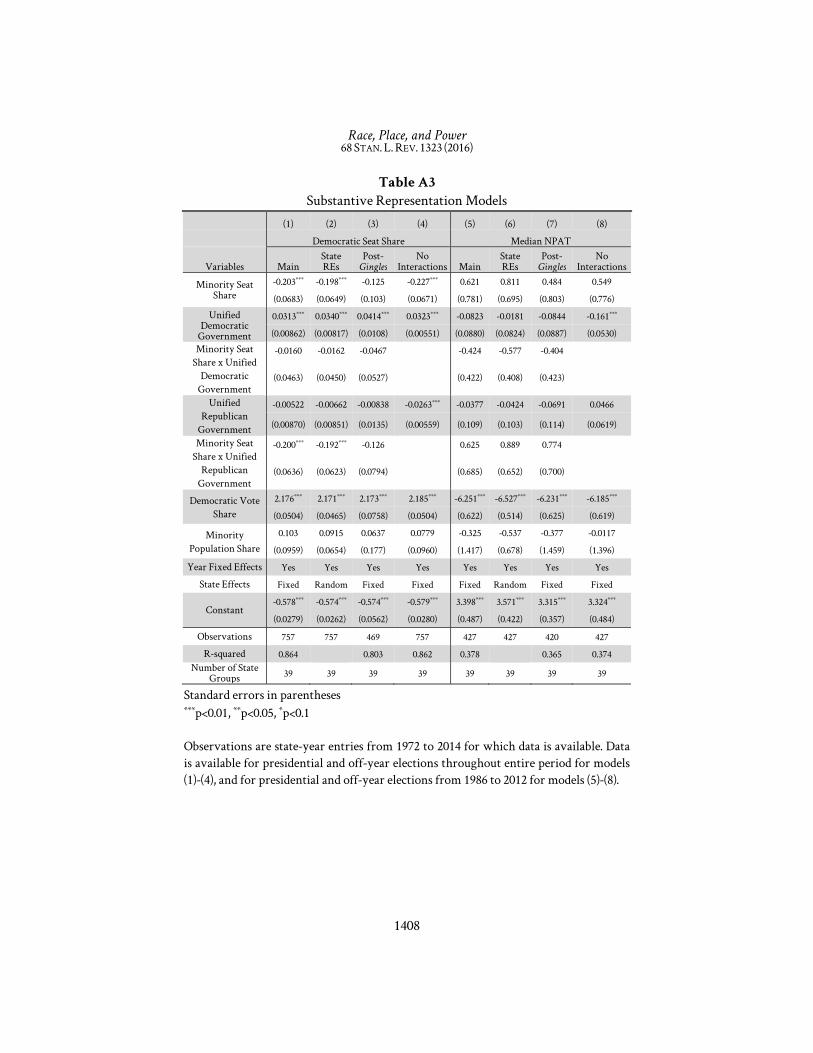
Race, Place, and Power 68 STAN. L. REV. 1323 (2016)
1408
Table A3 Substantive Representation Models
(1) (2) (3) (4) (5) (6) (7) (8) Democratic Seat Share Median NPAT
Variables Main State REs
Post-Gingles
No Interactions Main
State REs
Post-Gingles
No Interactions
Minority Seat Share
-0.203*** -0.198*** -0.125 -0.227*** 0.621 0.811 0.484 0.549
(0.0683) (0.0649) (0.103) (0.0671) (0.781) (0.695) (0.803) (0.776)
Unified Democratic
Government
0.0313*** 0.0340*** 0.0414*** 0.0323*** -0.0823 -0.0181 -0.0844 -0.161***
(0.00862) (0.00817) (0.0108) (0.00551) (0.0880) (0.0824) (0.0887) (0.0530) Minority Seat
Share x Unified Democratic
Government
-0.0160 -0.0162 -0.0467 -0.424 -0.577 -0.404
(0.0463) (0.0450) (0.0527) (0.422) (0.408) (0.423)
Unified Republican
Government
-0.00522 -0.00662 -0.00838 -0.0263*** -0.0377 -0.0424 -0.0691 0.0466
(0.00870) (0.00851) (0.0135) (0.00559) (0.109) (0.103) (0.114) (0.0619)
Minority Seat Share x Unified
Republican Government
-0.200*** -0.192*** -0.126 0.625 0.889 0.774
(0.0636) (0.0623) (0.0794) (0.685) (0.652) (0.700)
Democratic Vote Share
2.176*** 2.171*** 2.173*** 2.185*** -6.251*** -6.527*** -6.231*** -6.185***
(0.0504) (0.0465) (0.0758) (0.0504) (0.622) (0.514) (0.625) (0.619)
Minority Population Share
0.103 0.0915 0.0637 0.0779 -0.325 -0.537 -0.377 -0.0117
(0.0959) (0.0654) (0.177) (0.0960) (1.417) (0.678) (1.459) (1.396)
Year Fixed Effects Yes Yes Yes Yes Yes Yes Yes Yes
State Effects Fixed Random Fixed Fixed Fixed Random Fixed Fixed
Constant -0.578*** -0.574*** -0.574*** -0.579*** 3.398*** 3.571*** 3.315*** 3.324***
(0.0279) (0.0262) (0.0562) (0.0280) (0.487) (0.422) (0.357) (0.484)
Observations 757 757 469 757 427 427 420 427
R-squared 0.864 0.803 0.862 0.378 0.365 0.374 Number of State
Groups 39 39 39 39 39 39 39 39
Standard errors in parentheses ***p<0.01, **p<0.05, *p<0.1 Observations are state-year entries from 1972 to 2014 for which data is available. Data is available for presidential and off-year elections throughout entire period for models (1)-(4), and for presidential and off-year elections from 1986 to 2012 for models (5)-(8).