STANFORD GEOTHERMALPROGRAM

QUARTERLY REPORT

OCTOBER 1 – DECEMBER 31, 1996

1

1 AN EXPERIMENTAL STUDY OF BOILING IN POROUS MEDIA

This research project is being conducted by Dr. Cengiz Satik. The objective of this study isto improve our understanding of the process of boiling in porous media by using bothexperimental and numerical methods.

1.1 SUMMARY

The objective of this work is to improve the understanding of the process of boiling inporous media. The ultimate goal is to obtain the two important but currently unknownfunctions of relative permeability and capillary pressure functions. One horizontal and onevertical experiment were conducted using Berea sandstone core samples. Difficulties wereencountered in analyzing the results of the first preliminary boiling experiment: namely theapparent existence of a steam phase at inappropriately low temperatures. These resultssuggested several improvements to the design of the experimental apparatus. Upon thecompletion of these modifications, further horizontal and vertical experiments wereconducted. Three-dimensional porosity and steam saturation distributions were determinedusing an X-ray CT scanner. The maximum difference between the centerline and walltemperatures for the horizontal experiment was found to be less than 2 oC, therefore, wallmeasurements were shown to be adequate to represent the temperature of a circular slicealong the core. The steam saturation distributions calculated from the X-ray CT data didnot show a significant steam override in any of the experiments. Steady-state steamsaturation data showed a progressive boiling process with the formation of the threeregions of steam, two-phase and liquid as the heat flux was increased. The previousproblem of steam existing at inappropriate temperatures was not observed in the latervertical experiment. A comparison of the three-dimensional saturation profiles from bothexperiments showed a longer two-phase zone in the horizontal boiling case than that in thevertical case.

1.2 INTRODUCTION

The process of boiling in porous media is of significance in geothermal systems as well asin many other applications such as porous heat pipes, drying and nuclear waste disposal.Despite its importance in these applications, the fundamentals of this process are poorlyunderstood. Most of the problems arise from the lack of the understanding of themechanics and dynamics of this complex process.

A look at the previous literature shows that many attempts have been made in bothexperimental and theoretical directions to investigate and to describe the process of boilingin porous media (Satik, 1994). Most previous studies have used continuum formulationswhich made use of Darcy’s law extended to multiphase flow with relative permeability andcapillary pressure functions derived from isothermal gas-liquid displacement processes.These processes have major differences to boiling displacement which involves additionalphenomena such as heat transfer, nucleation and phase change. Moreover, the continuumapproaches are also limited by the assumption of capillary control at the pore level (low

2

Capillary and Bond numbers). Due to these restrictions and uncertainties, it is unclearwhether the relative permeability and capillary pressure functions currently used formodeling the process of boiling in porous media are appropriate.

At the same time, fundamental studies focusing at the microscopic pore scale have beenvery limited. In a recent study by Satik and Yortsos (1996), numerical and experimentalpore networks were used to model boiling in porous media at a microscopic pore scale.Satik and Yortsos (1996) developed a numerical pore network model for boiling in ahorizontal, two-dimensional porous medium and conducted visualization experiments byusing glass micromodels. Although progress was made, their model was developed onlyfor a single bubble growth problem in a horizontal porous medium, ignoring the effects ofgravity. Therefore, further work is still needed to improve the understanding and toresolve the issues raised by the continuum formulations (see Satik, 1994, for details) andeventually to obtain correct forms of the relative permeability and capillary pressurefunctions.

In this work, we used a different technique to study this problem. We conducted boilingexperiments with real core samples such as from Berea sandstone. Using an X-raycomputer tomography (CT) scanner, we visualized the process and determined the three-dimensional fluid distributions within the core while the experiment was in progress. Byusing thermocouples, pressure transducers and heat flux sensors under the control of adata-acquisition system, we obtained temperature, pressure and heat flux values along acore, respectively. The comparison of the experimental data with the results of a numericalsimulator will give us an opportunity to check the results Moreover, using an optimizationtool along with a numerical simulator combined with experimental results, the appropriateform of the relative permeability and capillary pressure functions can be obtained. Ourultimate goal is to be able to carry out these experiments with core samples taken fromThe Geysers geothermal field in California. Concurrent efforts are being directed towardsthe construction of an apparatus that can be used to carry out boiling experiments withlow permeability core samples.

This paper reports on the results of two experiments conducted using Berea sandstonecore samples. The core was positioned horizontally in the first experiment while it wasvertical in the second one. Two complete sets of experimental data were collected. Thesewill be discussed in detail here. The paper is organized as follows: We first describe theexperimental apparatus, discuss the procedure followed and finally present the results ofthe two experiments.

1.3 EXPERIMENTAL APPARATUS AND PROCEDURE

A schematic of the experimental apparatus is shown in Figure 1.1. The apparatus consistsof a core holder, a data acquisition system, a vacuum pump, a liquid pump and a balance.Ten pressure taps and thermocouples are placed along the core length to measure

3

pressures and temperatures, respectively. A heater and a heat flux sensor are placed in thespecially designed inlet end of the core holder. In addition, several heat flux sensors areplaced along the core to measure heat losses. During an experiment, the core holder isplaced inside the high resolution X-ray CT equipment to obtain in-situ saturation profilesalong the core. During CT scanning, an X-ray source is revolved around the object to takevarious projections at many angles and the data collected are then used to reconstruct theinternal image. The method causes an averaging of X-ray attenuation as X-ray beamstravel through the object while changes in density and/or thickness of the material causedifferences in X-ray attenuation (Johns et al., 1993).

Figure 1.1: Schematic of the experimental apparatus.

The experimental procedure is as follows. First, air inside the pore space is removed byvacuuming the core. The core is then scanned at predetermined locations to obtain dry-core CT (CTdry) values. Next, deaerated water is injected into the core. This stepcontinues until the core is completely saturated with water, at which time the core is X-rayscanned again at the same locations to obtain wet-core CT (CTwet) values. Also, pressurereadings are taken at this time to calculate the absolute permeability of the core. Steady-state boiling experiments mainly involve the injection of heat into the core at varyingpower levels. During the experiment, the heating end of the core is closed to fluid flowwhile the other end is connected to a water reservoir placed on a balance. The balance isused to monitor the amount of water coming out of the core during the process. The coreholder is covered with a 4 inch thick layer of insulation material to reduce the heat losses.In addition, several heat flux sensors are placed along the core to measure the actual heatlosses. Continuous measurements of pressure, temperature and heat flux are taken duringeach heat injection rate step until steady state conditions are reached. During the boilingprocess each step continues until the water production rate becomes zero, and thepressures, temperatures and heat fluxes stabilize; these are indications of steady-stateconditions. At the onset of steady-state conditions, the core is scanned again at the samelocations to obtain CT (CTexp) values corresponding to the particular heat flux value. Tocomplete the set of measurements, pressure, temperature and heat flux readings arerecorded again. The heat flux is then changed, and the full procedure is repeated. After theexperiment is completed, the porosity and saturation distributions are calculated from theCT values. More complete details of the calculation method were given in Satik et al.(1995).

4

The porosity distributions at various locations along the core are calculated by insertingCTdry and CTwet values into the following equation:

φ =−

−

CTwet CTdry

CTwater CTair(1.1)

where CTwater and CTair are CT numbers for water and air respectively.

Steam saturation distributions are also calculated by using the following equation:

Ssteam

CTwet CTexp

CTwet CTdry

=−

−

(1.2)

1.3 RESULTS

Two experiments were conducted using two different Berea sandstone core samples. Thecore sample was positioned horizontally in the first experiment while it was positionedvertically in the second experiment. Two complete sets of experimental data were obtainedfrom these experiments for the case in which the heat flux was increased. These includedporosity and saturation distributions determined using the X-ray CT data, and alsopressure, temperature and heat flux readings. The results obtained from these twoexperiments are discussed below.

The length and diameter of the cores used in both experiments were 43 cm and 5.04 cm,respectively. Before being used in each experiment, both cores were scanned using the X-ray CT scanner at various locations to ensure that they were free of inhomogeneties. Bothcores were found to have very similar X-ray CT images. By using the Darcy equation withthe results of the wet-core step during each experiment, the absolute permeability of bothcores was calculated to be around 500 md. During both experiments, we scanned a totalof 42 slices along the core. Using Equation (1.1) and dry and wet X-ray CT data, a three-dimensional porosity profile of each core was constructed. All of those slices for each coreindicated a fairly homogenous core. The porosity data were then averaged over eachcircular slice in order to obtain porosity profiles given in Figure 1.2. The figure shows auniform porosity distribution for both cores. The minimum, maximum and averageporosity values were calculated to be 0.196, 0.208 and 0.2012 for the first core and0.1826, 0.1881 and 0.1865 for the second core, respectively.

5

Recently, we reported the preliminary results from an earlier horizontal boiling experiment(Satik and Horne (1996). Rather unusual temperature profiles were found in theexperiment. Comparison of the steam saturation profiles obtained from the X-ray CTscanning with the corresponding temperature and pressure profiles indicated aninconsistency. The steam saturation profiles showed non-zero values up to temperaturesof as low as 50 oC. Although pressures were not measured during this experiment theywere assumed to be above atmospheric pressure since the outlet of the core wasconnected a water reservoir placed next to the core. This unusual behavior was initiallyattributed to air trapped inside porous medium and air dissolved in the water used tosaturate the porous medium (Satik and Horne, 1996). To remedy this problem, theexperimental procedure was changed to remove any possible preexisting gas phase in thesystem. During the new procedure, the core was first vacuumed to 0.00319 psi before theexperiment. The water used to saturate the core was then deaerated by preboiling it in acontainer.

0.17

0.18

0.19

0.2

0.21

0.22

0 10 20 30 40 50

Distance from heater, cm

Por

osi

ty

Vertical Boiling

Horizontal Boiling

Figure 1.2: Average porosity profiles along the core, calculated from X-ray CT dataobtained during both boiling experiments.

During the first experiment, in which the core was horizontal, the core was scanned andthree-dimensional porosity distributions were obtained eight times before and after heatingin order to observe the first formation of the steam phase. These three-dimensionalporosity distributions were then averaged over each circular cross-section of the core thatwas scanned in order to obtain the average porosity profiles, four of which are given inFigure 1.3. All of the curves displayed in the figure, except the curve at 2770 min, show afairly uniform porosity profile along the core and are within close proximity to each other.The deviation of the curve at 2770 min at distances closer to the heater suggests the firstappearance of the steam phase. The comparison of all eight porosity curves with pressureand temperature data indicated that a steam phase did not appear until the appropriateboiling temperature. This results is important because it confirms that air was successfullyremoved from both porous medium and the water used to saturate it.

6

Both boiling experiments were conducted by increasing the heater power settingincrementally to reach a desired heat flux value. Figure 1.4 shows the history of the heaterpower settings and the heat flux values obtained from heat flux sensors for both horizontaland vertical experiments. The same heater was used in both experiments, thus themagnitude of the power generated by the heater was similar in both cases at the samepower setting value.

0.09

0.11

0.13

0.15

0.17

0.19

0.21

0 10 20 30 40 50Distance from heater, cm

Po

rosi

ty

Before Heatingtime= 610 mintime= 1560 mintime=2770 min

Figure 1.3: Average porosity profiles along the core, obtained from the X-ray CTscanning conducted at four times during the horizontal boiling experiment.

During the horizontal experiment, we recorded both the centerline and wall temperaturesat ten locations along the core. The centerline temperatures were measured in thermowellsextending to the center of the core. The wall temperatures were measured over the outerlayer of the epoxy and next to the thermowells. In Figure 1.5, we show the comparison ofthe histories of the centerline and wall temperatures obtained at four locations along thecore length. The figure shows both transient and steady state (where the temperatureprofile flattens) sections of the temperature profiles at each heater power value. Themaximum temperature reached during the first experiment was 225oC. As shown in Figure1.5, the maximum difference between the two temperature profiles was less than 2oC. Thissuggested that the radial temperature gradient along the core was not significant for thisset of experimental conditions and therefore it would be adequate to measure walltemperatures only.

7

0

1000

2000

3000

4000

5000

6000

7000

0 1000 2000 3000 4000 5000

Time elapsed, minH

eat

flux,

W/m

^2

0

20

40

60

80

100

Hea

ter

Pow

er S

ettin

g, %

Heat Flux Reading

Heater Power Setting

(a)

0

500

1000

1500

2000

2500

3000

3500

4000

4500

0 1000 2000 3000 4000 5000 6000 7000 8000

Time elapsed, min

Hea

t F

lux

, W/m

^2

0

20

40

60

80

100

Hea

ter

Po

wer

Set

tin

g, %

Heat Flux Reading

Heater Power Setting

(b)

Figure 1.4: Heater power settings and corresponding heat flux values obtained from theheat flux sensor: (a) horizontal experiment, (b) vertical experiment

The core was scanned several times to obtain three-dimensional steam saturationdistributions during the experiment. These three-dimensional steam saturation distributionswere then averaged over each circular cross-section of the core that was scanned in orderto obtain the average steam saturation profiles. In Figure 1.6, we show four of thesesaturation profiles. The saturation profile at 2770 min shows a two-phase (steam andwater) zone followed by a completely water-filled zone while the profile at 5130 minshows three distinct regions of completely steam, two-phase and completely water. Asexpected, the steam saturation is higher at locations closer to the inlet, where the heater islocated, and decreases towards the outlet.

8

0

20

40

60

80

100

120

140

0 1000 2000 3000 4000 5000Time elapsed, min

Tem

per

atu

re, C

Tw2

Tw3

Tw4

Tw5

Tc2

Tc3

Tc4

Tc5

Figure 1.5: Comparison of the histories of four centerline and wall temperatures duringthe horizontal boiling experiment.

0

0.2

0.4

0.6

0.8

1

0 10 20 30 40 50

Distance from heater, cm

Ste

am S

atu

rati

on

time= 1560 min

time= 2770 min

time= 3970 mintime= 5130 min

Figure 1.6: Average steam saturation profiles along the core, calculated from X-ray CTdata during the horizontal experiment.

The comparison of the saturation profile with the corresponding centerline temperatureprofile at 5130 min is shown in Figure 1.7. Steam saturation at 100oC is about 56% andvanishes at about 52oC. This suggests that the previous problem of the apparent existenceof a steam phase at inappropriate temperatures still existed. This behavior was alsoobserved on the other profiles obtained at different.

Following the horizontal experiment, another experiment was conducted with the coreholder positioned vertically to study the effect of gravity on the results. Since the coreused for the horizontal experiment had developed extensive cracks during the coolingstage, another core that had similar properties was prepared and used for the verticalexperiment. This experiment was also carried out by varying the heater power setting from20% to 70% incrementally (Figure 1.4b). Again, to ensure the removal of any gas phaseexisting in the porous medium or dissolved in the water saturating it, the procedureemployed in the first experiment was also used in the vertical experiment.

9

Time= 5130 min

0

0.1

0.2

0.3

0.4

0.5

0.6

0.7

0.8

0.9

1

0 10 20 30 40 50

Distance from heater, cmS

team

Sat

urat

ion

0

20

40

60

80

100

120

140

160

180

Tem

pera

ture

, C

Steam SaturationTemperature

Figure 1.7: Comparison of the steam saturation and temperature profiles along the coreduring the horizontal boiling experiment.

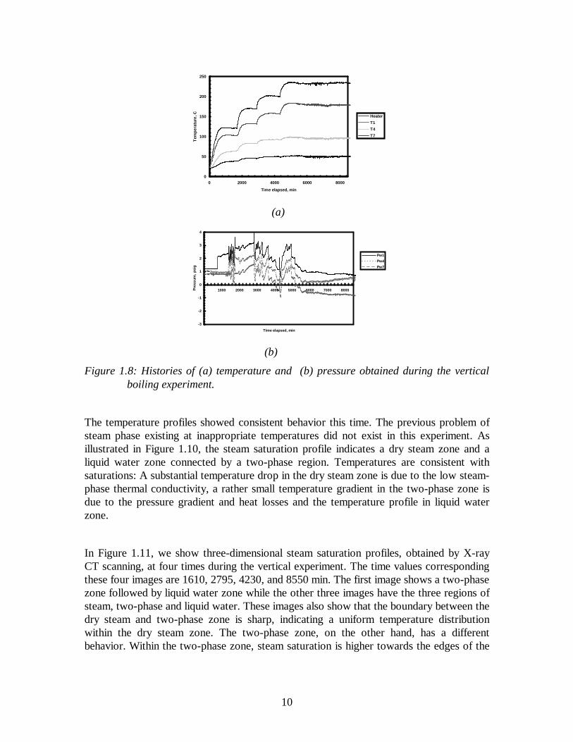
Measurements of temperature and pressure were taken at ten locations along the coreduring the experiment. The temperature profiles in Figure 1.8a show the transient andstabilization stages of each power change. On the other hand, the pressure profiles seem toexhibit an oscillatory behavior until about 5500 min at which time they start to stabilize(Figure 1.8b). Although not recognizable due to the scale of the graph in Figure 1.8a,these oscillations also exist in the temperature profiles.

In Figure 1.9, we show pressure, temperature and saturation profiles obtained at fourtimes during the vertical experiment. Each profile was obtained at the onset of steady-stateconditions after each time the heater power was changed. At the beginning of the heating(the curves at 0.022 min), temperatures, pressures and steam saturations along the corewas at room temperature, hydrostatic pressure and zero, respectively. After the heaterpower was increased to 50% (see also Figure 1.4b) temperatures close the heater startedto raise (Figure 1.8a). The saturation profile at 1610 min shows about 60% steamsaturation at the closest location to the heater. The corresponding pressure profile isconsistent with the saturations, showing higher pressures closer to the heater that may alsoindicate the formation of steam phase. As the heater power was increased further, dry-outconditions occurred, leading to existence of the three zones of dry steam, two-phase andliquid water zones (profiles at 2795, 4230 and 8550 min). However, the pressure profilesat 4230 and 8550 min show an unusual behavior, a decrease at all locations along the core.Currently we do not understand the cause of this pressure drop but it could be attributedto a small leak in the core or to a complication with pressure transducers. The pressuresincreased again during the cooling stage of the experiment, indicating a possible problemwith the pressure transducers. To improve the accuracy of pressure measurements in theexperiments, the acquisition of more accurate pressure transducers is in progress.

10

0

50

100

150

200

250

0 2000 4000 6000 8000

Time elapsed, minT

emp

era

ture

, C Heater

T1

T4

T7

(a)

-3

-2

-1

0

1

2

3

4

0 1000 2000 3000 4000 5000 6000 7000 8000

Time elapsed, min

Pre

ssu

re,

psi

g

Pw1

Pw4

Pw7

(b)

Figure 1.8: Histories of (a) temperature and (b) pressure obtained during the verticalboiling experiment.

The temperature profiles showed consistent behavior this time. The previous problem ofsteam phase existing at inappropriate temperatures did not exist in this experiment. Asillustrated in Figure 1.10, the steam saturation profile indicates a dry steam zone and aliquid water zone connected by a two-phase region. Temperatures are consistent withsaturations: A substantial temperature drop in the dry steam zone is due to the low steam-phase thermal conductivity, a rather small temperature gradient in the two-phase zone isdue to the pressure gradient and heat losses and the temperature profile in liquid waterzone.

In Figure 1.11, we show three-dimensional steam saturation profiles, obtained by X-rayCT scanning, at four times during the vertical experiment. The time values correspondingthese four images are 1610, 2795, 4230, and 8550 min. The first image shows a two-phasezone followed by liquid water zone while the other three images have the three regions ofsteam, two-phase and liquid water. These images also show that the boundary between thedry steam and two-phase zone is sharp, indicating a uniform temperature distributionwithin the dry steam zone. The two-phase zone, on the other hand, has a differentbehavior. Within the two-phase zone, steam saturation is higher towards the edges of the

11

core while the water saturation is higher closer to the centerline of the core, indicating apossible two-phase convection.

0

20

40

60

80

100

120

140

160

180

0 5 10 15 20 25 30 35 40 45

Distance from heater, cm

Tem

per

atu

re, C

time= 0.022 min

time= 1610 min

time= 2795 min

time= 4230 min

time= 8550 min

(a)

-1.5

-1

-0.5

0

0.5

1

1.5

2

2.5

3

3.5

0 10 20 30 40 50

Distance from heater

Pre

ssu

re, p

sig

time= 0.022 mintime= 1610 mintime= 2795 mintime= 4230 mintime= 8550 min

(b)

0

0.1

0.2

0.3

0.4

0.5

0.6

0.7

0.8

0.9

1

0 5 10 15 20 25 30 35 40 45

Distance from heater, cm

Ste

am S

atur

atio

n

time=1610 min

time=2795 min

time=4230 min

time=8550 min

(c)

Figure 1.9: Steady state (a) pressure, (b) temperature and (c) steam saturation profilesalong the core, obtained during the vertical boiling experiment.

Finally, in Figure 1.12 we show a comparison of the steam saturation profiles of bothhorizontal and vertical experiments at the same power values. These results show theeffect of gravity. In the horizontal case, the length of the dry steam zone is shorter and the

12

two-phase zone is longer than those in the vertical case. These results are expected sincethe two-phase zone, which has large compressibility, is expected to shrink in the verticalcase simply due to the gravity of the liquid layer overlaying it.

1.4 CONCLUDING REMARKS

Two boiling experiments were conducted by using Berea sandstone core samples: onewith a horizontal core and another with a vertical core. In a previous paper (Satik andHorne, 1996), we reported on the results of the first preliminary horizontal boilingexperiment during which we observed an inconsistency in the apparent existence of asteam phase at inappropriately low temperatures. Analysis of the results suggested severalimprovements on the design of the experimental apparatus and procedure (Satik andHorne, 1996). With the new apparatus and procedure, one horizontal and one verticalexperiment were conducted. Using an X-ray CT scanner, three-dimensional porosity andsteam saturation distributions were obtained during the experiments. Temperatures,pressures and heat fluxes were also measured. In the new experimental method, both thecore and the water used to saturate it were deaerated before the experiments. Bothcenterline and wall temperatures were measured during the horizontal experiment. Themaximum difference between the centerline and wall temperatures was found to be lessthan 2oC, hence the wall temperatures were found to be adequate to represent thetemperature of a circular slice along the core. Steady-state steam saturation distributionsshowed a progressive boiling process with the formation of the three regions of steam,two-phase and liquid as the heat flux was increased. The steam saturation distributionsobtained using the X-ray CT data did not indicate any significant steam override in eitherexperiment. The previous problem of steam existing at inappropriate temperatures was notobserved in the vertical experiment although it persisted to a small extent in the horizontalcase. The cause of this effect is still undetermined. Comparison of the three-dimensionalsaturation profiles from both experiments indicated a longer two-phase zone in thehorizontal case than that in the vertical case. This result is expected since the two-phasezone has higher compressibility. Pressure data obtained from both experiments indicatedpossible problems with pressure transducers. Improvements to the accuracy of thepressure measurements are currently in progress.

time=4230.007 min

0

0.1

0.2

0.3

0.4

0.5

0.6

0.7

0.8

0.9

1

0 5 10 15 20 25 30 35 40 45

Distance from heater, cm

Ste

am S

atu

rati

on

0

20

40

60

80

100

120

140

160

Tem

per

atu

re, C

Steam Saturation

Temperature

Figure 1.10: Comparison of the steam saturation and temperature profiles along the coreduring the vertical boiling experiment

13

Figure 1.11: Three-dimensional steam saturation distributions along the core, calculatedfrom the X-ray CT data obtained at four times during the vertical experiment.

14

0

0.2

0.4

0.6

0.8

1

0 10 20 30 40 50

Distance from heater, cmS

team

Sat

ura

tio

n

Horizontal Boiling at 70% power

Vertical Boiling at 70% power

Horizontal Boiling at 50% power

Vertical Boiling at 50% power

Figure 1.12: Comparison of the steam saturation profiles obtained at the same heaterpower values during the horizontal and vertical experiments.

15

2 INJECTION INTO GEOTHERMAL SYSTEMS

This work has been conducted by Program Manager Prof. Shaun D. Fitzgerald, VisitingProfessor Andrew W. Woods and Undergraduate Research Assistant Catherine Tsui-LingWang. This quarter, we present the results of a suite of experiments which have beenperformed in order to determine the effects of injection into geothermal reservoirs. Theresults obtained from the experiments are compared with theoretical predictions of theevolution of temperature profiles within a geothermal reservoir following the injection ofsupercooled liquid. For the case of constant rate liquid injection in an axisymmetricgeometry into a liquid-filled porous medium, we find that at slow rates of injection heat isconducted from the far-field towards the source. However, at higher rates of injection, anisothermal zone develops close to the injection well.

We conducted an experiment in which liquid was injected into a porous slab initially filledwith superheated vapor. We compared the evolution of the temperature profile within thesystem with the theoretical prediction (Woods and Fitzgerald, 1997) and found that asharp interface may develop between the liquid- and vapor-filled regions.

Finally, we investigated the injection of liquid into a fracture which initially containssuperheated vapor. We compared the evolution of the temperature profile within thefracture with a numerical prediction obtained from TOUGH2 (Pruess, 1991). It was foundthat a broad two-phase region exists between the completely liquid-filled and vapor-filledzones of the system.

2.1 INTRODUCTION

As geothermal reservoirs are exploited for power production or district heating, theybecome depleted and reservoir pressures fall. As a result of the potential significantreduction in well flow rates, injection is now viewed as a strategic element of anexploitation program for a geothermal reservoir. The additional pressure support that ispossible through the reinjection of spent brine can help minimize the reduction in pressure.However, although the potential benefits of additional pressure support by injection arelarge, there is a risk of breakthrough of cooler injected fluid at the production wells. Ifcold fluid reaches a production well the effects can be devastating. The specific enthalpyof the produced fluid falls. This leads to an increase in the average density of fluid within aproduction well, and therefore, the flowrate also decreases. The ability to predict the timeat which injected cold fluid reaches a production feed zone is important and a number ofmodelling studies have been performed aimed at determining the evolution of thetemperature profile within a reservoir following the onset of injection (Pruess et al., 1987;Woods and Fitzgerald, 1993, 1996, 1997).

In this report we present the results obtained from a series of analogue laboratoryexperiments which were performed to investigate liquid injection into geothermal

16

reservoirs. We first discuss the case of liquid injection into a liquid-filled porous mediumand compare the experimental findings with the predictions obtained from a theoreticalmodel (Woods and Fitzgerald, 1996). We then present the results obtained from anexperiment in which liquid was injected into a porous medium initially filled withsuperheated vapor. The evolution of the temperature profile within the system is found toagree with the theoretical model proposed by Woods and Fitzgerald (1996). Finally, weconsider the case of liquid injection into a fractured system. The experimental findings arecompared with predictions obtained from a numerical model TOUGH2 that was modifiedto enable us to model the boiling of ether within the fracture.

2.2 LIQUID INJECTION INTO A LIQUID-FILLED POROUS MEDIUM

We have performed a series of experiments to test the model of liquid injection into aporous layer developed by Woods and Fitzgerald (1996). In the first suite of experiments,the apparatus consisted of a cylindrical bed of consolidated permeable sand, of radius35cm and 3cm deep enclosed between two impermeable layers of epoxy resin. The sandbed consisted of 82% 30 mesh sand and 18% Portland cement. Twelve thermocoupleswere embedded into the sand layer at approximately 1cm radial intervals from the centralinjection port and these were connected to a digital data recorder. Before eachexperiment, carbon dioxide was injected into the center of the apparatus in order todisplace the air. Cold de-ionized water was subsequently injected in order to displace thecarbon dioxide. Any remaining CO2 dissolved in the water. Insulating material was thenplaced on the upper and lower surfaces of the epoxy boundaries and the apparatus wasconnected to a water pump and heater.

In each experiment water was supplied at a constant rate, which was varied fromexperiment to experiment in the range 5-50 ml/min. For convenience, hot water wasinjected into a cold liquid-filled sand bed and several experiments were conducted usingdifferent flow rates and injection temperatures. The primary advantage of using a sand bedfilled with liquid at room temperature, rather than at an elevated temperature, was that therisk of exsolution of any dissolved gases at room temperature was minimized. Aftercompletion of the experiments two CT scans of the sand layer apparatus were taken, onewith the core fully dry and one with the core fully saturated with liquid. Using thesemeasurements, the porosity φ was estimated to be 35+/-3%. Using this estimate togetherwith the known properties of the sand, the effective thermal diffusivity of the porousmedium was calculated to be 1.3+/-0.1E-06m2/s. During each experiment, temperaturemeasurements were recorded every 5s.

We wish to use the results obtained from these experiments in order to test the theoreticalprediction proposed by Woods and Fitzgerald (1996). In this regard we developed asimilarity type solution for the evolution of the temperature profile as a function of radiusand time for the case in which liquid is injected at a constant rate 2ΠQ from a centralsource in an axisymmetric geometry. Following the theory of Woods and Fitzgerald(1996, 1997), the temperature profile is expected to develop according to

17

T η( )= To + ∆T ηλw β−1

0

η∫ exp −η2( )dη (2.1)

where β=Q/κ,

∆ = T2 − T0( )/ ηλwβ −1

0

∞∫ exp −η2( )dη (2.2)

T0 is the source temperature, T2 is the far-field temperature, λw=ρlCpl/(φρlCpl+(1-φ) ρrCpr),ρl and ρr are the densities of liquid water and rock respectively, Cpl and Cpr are the specificheat capacities of liquid and rock, and κ is the average thermal diffusivity of the liquid-filled porous medium.

In Figure 2.1 we compare the temperature profiles obtained in an experiment with thetheoretical predictions for the case β=0.67 and β=3.4. The radial locations of thesemeasurements have been non-dimensionalized η=r/(2κt)1/2 and the temperature profiles areshown as a function of η. For both the fast injection case β=3.4 and the slower injectioncase β=0.67, the experimental results collapse accurately onto the theoretical temperatureprofiles.

The experimental data confirms the theoretical prediction that at low flow rates (β<1/λw,Figure 2.1(i)), the isotherms are advected more slowly than the rate of conduction, so theinternal boundary layer extends back to the source. However, at high flow rates (βλw>1,Figure 2.1(ii)), the liquid is heated to the far-field temperature by cooling the rock near thesource.

We now extend our discussion to investigate the case of liquid injection into a porousmedium initially containing superheated vapor.

2.3 LIQUID INJECTION INTO A VAPOR-FILLED POROUS MEDIUM

Following the exploitation of a number of geothermal reservoirs such as The Geysers,there now exist zones in which the reservoir pressure is below the local saturation pressurecorresponding to the reservoir temperature. These regions are prime candidates for theinjection of liquid since it is in these regions that the pressure has usually declined mostsignificantly, thereby leading to dramatic decreases in flow rate from the production well.In addition, the reduction in pressure and formation of reservoir superheat has created thepossibility for injection of fluid and subsequent vaporization of this fluid. We now extendthe experimental techniques developed in the previous section to the case in which ananalogue reservoir initially contains superheated vapor.

18

20

25

30

35

40

45

50

55

60

0.1 1 10

E

E

1 min

2 min

3 min

10 min

20 min

30 min

tem

pe

ratu

re (

oC

)η

β=0.68

(i)

20

30

40

50

60

0.1 1 10 100

1 s10 s20 s30 s100 s200 s300 s1000 s1500 sDD

tem

pe

ratu

re (

oC

)

η

β = 3.42

(ii)

Figure 2.1 Comparison of the model predictions with experimental measurements oftemperature as a function of distance from the source. Distances are shown indimensionless form η=r/(2κt)1/2. Results are shown for two experiments in whichhot liquid is injected into a cold water saturated layer. (i) β=0.67, T(input)=63C and T(initial)=20.2 C and (ii) β=3.42, T(input)=59 C and T(initial)=21 C.Symbols show the temperature at different times during the experiment. Thesolid lines correspond to the theoretical prediction.

The apparatus used in these experiments consisted of a slab of 500 md, 15.5% porosityBerea sandstone, 12in in diameter and 0.95in thickness. The sandstone core was initiallyheated in an oven to 500oF for 24 hours in order to deactivate the clays. This wasperformed in order that during the injection experiments, the clays did not swell andthereby block the pores. 12 thermocouples were then placed at various distances from thecenter of the disk and a central injection port was also drilled. The thermocouple holeswere aligned along three radial transects and were drilled to a depth of 0.475in so that thethermocouples recorded the temperatures at the center of the slab. Epoxy resin wasapplied to the upper and lower surfaces of the sandstone core to form impermeableboundaries and the core was then flooded with carbon dioxide.

19

In order to study the boiling of liquid within the porous medium, the apparatus was heatedin a oven at 108oC for several hours. The apparatus was then removed from the oven, laidhorizontally on insulating material and covered with additional pieces of insulation.Deionized water which had been heated to approximately 75oC was then pumped throughthe injection port at a rate of 10ml/min. Temperatures were recorded every 5s by a digitaldata recorder.

Woods and Fitzgerald (1996, 1997) presented a theoretical model for the evolution of thesystem as liquid is injected at a constant rate into a porous medium in an axisymmetricgeometry. In this model, the temperature profile is also described by a similarity solution interms of the variable η=r/(2κt)1/2. The theoretical prediction obtained from Woods andFitzgerald (1996, 1997) is plotted in Figure 2.2 with the experimental data.

70

75

80

85

90

95

100

105

110

0 1 2 3 4 5

η

Figure 2.2 Temperature as a function of η for an experiment in which water was injectedat 73oC into a sandstone core initially at 108oC. The injection rate of 10ml/mininto a core 0.95in thick corresponded to the case β=0.67. Symbols represent theexperimental data and the solid line indicates the theoretical prediction. Eachset of symbols corresponds to temperatures obtained from one thermocouple.

The temperature profiles within both the liquid- and vapor-filled regions are in closeagreement with those predicted from the theory. Furthermore, the interface between theliquid- and vapor-filled zones is found to be sharp, in accord with the theoretical model.However, there are some noticeable discrepancies. In particular, the experimental dataindicates that the temperature does not necessarily increase monotonically with radius awayfrom the injection port. 12 thermocouples were used in the experiment, 4 thermocouplesaligned along 3 different radial segments. The variation in temperature along each line of 4thermocouples indicated that the boiling interface did not propagate as a circular front. If theapparatus was not perfectly level, then a non-circular front would be expected. However, weare reasonably confident that the apparatus was level. Propagating boiling fronts can becomeunstable if the fraction F which boils is sufficiently high (Fitzgerald and Woods, 1994).

20

However, in the present experiment the fraction which boiled was approximately 7% which ismuch less than the critical value. As a result, it is likely that the departures in temperatureaway from the theoretical prediction were caused by heterogeneities in the permeability of thesandstone core. Even though the scatter in the data indicates that the interface did notpropagate uniformly, the general agreement between the experimental data and the theorysuggests that the theory is valid over length scales greater than the scale of non-uniformity ofthe front.

The close agreement between the experimental data and model predictions for injection intoporous media is comforting. However, geothermal reservoirs can also contain extensive zonesof fractured rock. We have therefore extended our study of liquid injection into superheatedrock to investigate the effects of injection into an isolated fracture.

2.4 LIQUID INJECTION INTO A VAPOR-FILLED FRACTURE

In the case of liquid injection into a porous medium filled with superheated vapor, the amountof heat which can be extracted from the rock and used for vaporization is a function of theextent of cooling which occurs at the vaporization front and the amount of heat which isconducted towards the point of injection. The heat required to overcome the latent heat ofvaporization is supplied by the rock grains within the vapor-saturated thermal boundary layerimmediately ahead of the liquid-vapor interface. However, in the case of a fractured system,the heat is supplied by conduction from the fracture walls perpendicular to the flow. In orderthat boiling may occur, the heat required to overcome the latent heat of vaporization must besupplied over a finite area. As a result, boiling has to occur over a broad two-phase zonerather than a sharp interface. This is in contrast to the case of injection into a porous mediumat low degrees of superheat, where the liquid-vapor transition zone can be a narrow interface.

In order to develop a quantitative model of this scenario we have used the TOUGH2 generalpurpose numerical code (Pruess, 1991) for solving the coupled equations of heat and massconservation in a fractured-porous type geothermal reservoir. In addition we have conducteda series of experiments in which liquid ether was injected at rates of 10-20 ml/min into ahorizontal rough-walled fracture in order to determine whether a two-phase zone does indeeddevelop as predicted. Ether was chosen as the working fluid since it boils at 34.5oC atatmospheric pressure thereby enabling us to study the boiling process using fracturetemperatures of 50-90oC. In Figure 2.3 we show a series of photographs taken at varioustimes during the course of one experiment as ether was injected at constant rate. As the ethermigrated radially out into the fracture, a liquid zone developed close to the injection port.Ahead of this zone a two-phase region developed. The leading (front) edge of the two-phasezone is shown in Figure 2.3 by the region of concentrated dye. The orange dye used was onlysoluble in the liquid phase of ether and therefore accumulated at the edge of the boiling zoneas shown. The front was observed to remain roughly circular. The present experimental resultsprovide a reliable data set to test the numerical prediction of TOUGH2. The numericalproblem considered for comparison with the experimental observations was a two-dimensionalradial system with semi-infinite fracture walls.

21

Figure 2.3 The spreading of dyed ether as it is injected at 20ml/min. The times showncorrespond to times 10, 15, 75 and 180s after the onset of injection. The regionof concentrated dye indicates the leading (front) edge of the two-phase boilingzone.

22

20

25

30

35

40

45

50

55

60

65

0 2 4 6 8 10 12

Radius (cm)

50 sec April 29 April 30 May 3 August 16

20

25

30

35

40

45

50

55

60

65

0 2 4 6 8 10 12

Radius (cm)

200 sec April 29 April 30 May 3 August 16

20

25

30

35

40

45

50

55

60

65

0 2 4 6 8 10 12

Radius (cm)

500 sec April 29 April 30 May 3 August 16

20

25

30

35

40

45

50

55

60

65

0 2 4 6 8 10 12

Radius (cm)

1400 sec April 29 April 30 May 3 August 16

Figure 2.4 Temperature profiles at times 50, 200, 500 and 1400s after the onset ofinjection of 21oC liquid ether at 10 ml/min into a fracture originally at 64oC.The symbols represent data obtained from different experiments and the solidline indicates the profile obtained from the modified numerical code TOUGH2.

In order to compare the numerical prediction of the code with the experimental results, thecode was modified to incorporate the physical properties of ether rather than water for the

23

reservoir/apparatus fluid. For example, properties of ether at atmospheric conditionsinclude: vapor density 3.331kg/m3, liquid density 713.8kg/m3, latent heat of vaporization377.7kJ/kg, vapor viscosity 8.4e-6 kg/sm and liquid viscosity 1.66e-4 kg/sm (Weast,1972).

We found that heat was transferred from the brass injection port to the liquid ether. Inorder to account for this additional heat transfer we placed a thermocouple within thefracture at the point of entry of the fluid. As the experiment proceeded the inlettemperature of the liquid ether to the fracture decreased as expected. Therefore, the inlettemperature of the liquid used in the numerical fracture model was reduced at varioustimes in accord with the experimental observations.

Experiments were conducted at flow rates of 10 and 20 ml/min. Typical temperatureprofiles at various times for 10 ml/min are shown in Figure 2.4. It is seen that theagreement between the experimental observations and the numerical predictions is good.Close to the injection port a liquid-filled region develops as predicted. Within this liquid-filled zone the experimental data is in very close agreement with the numerical prediction.The radial temperature and temperature gradient increase away from the injection site untilboiling conditions are attained. Ahead of the liquid zone lies a two-phase zone. The scatterof the experimental data becomes greater towards the leading edge of the two-phase zone.During the course of the experiments it was found that the leading edge of the boilingzone tended to pulse rather than migrate steadily. As a result, the temperature may havefluctuated whereas the numerical prediction did not indicate this phenomenon. Theseexperimental results suggest that the predictions for the evolution of the temperature,pressure and saturation distributions which one may obtain from TOUGH2 are likely to bevery accurate for uniform horizontal fractures bounded by impermeable rock.

2.5 CONCLUSIONS

We have conducted a series of laboratory experiments in order to test the theoreticalmodels of liquid injection into a liquid-filled or superheated porous medium type reservoir(Woods and Fitzgerald, 1993, 1996). In the case of liquid injection into a liquid-filledporous medium we found that at low flow rates, the temperature increases immediatelyfrom the injection port in accord with the theory. However, at higher flow rates, anisothermal zone develops close to the inlet site. The liquid is heated to the far-fieldtemperature by cooling the rock close to the source.

We have also performed an experiment in which liquid was injected into a porous rockinitially filled with superheated vapor. In this case a sharp interface between the liquid- andvapor-filled regions develops. The amount of heat available for vaporization depends uponthe difference in the amount of heat conducted from the vapor-filled zone towards theinterface and that conducted away from the interface into the liquid-filled zone. The

24

experimental results indicate that the theoretical treatment of injection proposed by Woodsand Fitzgerald (1996, 1997) is accurate.

We then investigated the case in which liquid is injected into a fracture bounded byimpermeable rock in order to ascertain the primary differences between heat transfer andboiling within porous media and fractured systems. It was found that a broad two-phasezone formed within the fracture in order that boiling could occur. This is in contrast to thecase of boiling in a porous medium where a sharp interface formed between the liquid- andvapor-filled zones.

We are in the process of developing this work further and will examine experimentallyhow an injection plume migrates under gravity and how the rate of propagation of the coldwater changes when the rock bounding the fracture is permeable.

25

3 MEASUREMENTS OF STEAM-WATER RELATIVEPERMEABILITY

This project is being conducted by Research Assistant Raul Tovar, Dr. Cengiz Satik andProfessor Roland Horne. The aim of this project is to measure experimentally relativepermeability relations for steam and water flowing simultaneously in a porous medium.

3.1 SUMMARY

During the quarter, a set of relative permeability relations for simultaneous flow of steamand water in porous media measurements were attempted in steady state experimentsconducted under conditions that eliminate most errors associated with saturation andpressure measurements. However, while attempting to measure them the two coressamples used started leaking at the core-epoxy inlet interface. In this report we show theresults obtained before the onset of core failure.

3.2 EXPERIMENTAL APPARATUS

The experimental apparatus consisted of an injection unit and a core holder made ofepoxy. The injection unit consisted of two furnaces to generate steam and hot water. Twopower controllers were used to control the energy supplied by each of the two furnaces.Heat losses along the core body were measured by using eight heat flux sensors.Temperatures were measured by seventeen thermocouples, nine of which were J-typethermocouples, placed along the steam injection, water injection and sink lines. Theremaining eight T-type thermocouples and the eight heat flux sensors were placed at equalintervals along the core body. Pressures were measured by using seventeen pressure

Pressure ports

Heat flux sensors

and thermocouples

Thermocouples and pressure ports

To sinkPumps

Steam generator

Hot water generator

Zoom areaHot plate

Signal Conditioning

Cooling container

PC

Insulation

CORE HOLDER

Figure 3.1 Experimental apparatus.

26

taps placed next to the thermocouples.

The proportional voltage signals from the heat flux sensors, thermocouples and pressuretransducers were first conditioned and then they were collected by a data acquisitionsystem. The data was then analyzed in a personal computer using “LABVIEW“, agraphical programming software.

The core (Berea sandstone) samples used for these experiments were 43.18 cm in lengthand 5.08 cm in diameter. During the preparation of a core holder, core samples were firstheated to 450oC for twelve hours to deactivate clays and to get rid of residual water.Eight ports to measure temperatures and pressures were next fitted at fixed intervalsalong the edge of the core before the rest of the core was covered completely by a hightemperature epoxy. The core was tested for leaks before being covered with an insulationmaterial made of ceramic blanket. Experiments were conducted inside a high-resolutionX-ray CT scanner so that in-situ saturations could be measured while the experiment wasin progress.

Air initially dissolved in the water would give erroneous saturation readings, so air wasremoved by boiling and cooling the water before injecting into the core, as shown inFigure 3.1. Also, the core was evacuated using a vacuum pump to get rid of the airtrapped inside the pore space.

3.3 CALCULATIONS

Mass flowing fractions can be calculated by applying the following mass and energyconservation equations:

m m mt v l= + (3.1)

m h m h m h Qv v l l t t+ = + (3.2)

where m andh denote mass flow rate and enthalpy, respectively, and the subscript t refersto total, v to vapor phase and l to the liquid phase. Q is the total heat lost upstream of thepoint being considered.

To apply these equations to the control volume shown in Figure 3.2, at point 1superheated steam is injected at a know rate m1, pressure p1 and temperature T1. At thesame time sub-cooled water is injected at point 2 at a know rate m2, pressure p2 andtemperature T2. From T1 and p1 using the steam table for superheated conditions we caninterpolate to obtain h1v. From T2 and using the steam table saturated for saturatedconditions we can approximate h2 by using h2l, the enthalpy at the saturated liquid phase.At point 3, when saturation is reached, either from p3 or T3 using saturated steam tableswe can obtain h3l and h3lv., the liquid phase enthalpy and the latent heat of vaporizationrespectively. Q is obtained by using Q”, the heat flux sensor value:

Q Q A= " (3.3)

where A is the surface area of the core from point 1 (or point 2) to point 3.

27

Control volumePoint 1

Point 2 Point 3Heat flux sensor and thermocouple

Pressure port

Steam line

Hot water line

y

x

Point 1

Point 2Point 3

x

y

core

Figure 3.2 Control volume from Figure 3.1 zoom area.

Thus Equation (3.1) becomes:

m m m3 1 2= + (3.4)

and (3.2) becomes:

m h m h m h Q Av l1 1 2 2 3 3+ = + " (3.5)

where:

h h xhl lv3 3 3= + (3.6)

Thus the steam fraction x in the flow at any time can be calculated by

xm h m h Q A

m h

h

hv l

lv

l

lv

=+ −

−1 1 2 2

3 3

3

3

"(3.7)

Then the relative permeabilities to steam and water can be calculated by the correspondingDarcy equations for each phase in terms of the mass flow rates

kx m

kAp

x

rlt l l= −

−( )1 µ ν∆∆

(3.8)

and

kxm

kAp

x

rst s s= −µ ν∆∆

(3.9)

28

3.3 PRELIMINARY RESULTS

Two core samples were used to generate the following results. Core sample 1 failedbefore any meaningful X ray CT scan could be taken.

Figure 3.3 shows absolute permeability measured over a time interval of 250 minutes forcore sample 1. Each curve represents measurements taken at different temperatures witha constant flow rate. The curves seem to indicate that there is no major variation inpermeability as a function of temperature. The variation shown is most probably causedby the precision of the pressure transducers used to measure pressure in the experiment.

Figure 3.4 shows absolute permeability measured over a time interval at differenttemperatures and flow rates for core sample 2. This figure once again does not show anappreciable variation or permeability with respect to flow nor temperature with theexception of a hike at the third point (about 20 minutes) for the curve with an averagepermeability of 684 md. The curve with an average permeability of 661 md was obtainedas the core was heated from 39 oC to 88 oC in a period of 250 minutes.

The pressure drop between the first and the last pressure ports (see Figure 3.1), separatedby a distance of 35 cm, was used to calculate the permeabilities shown in Figures 3.3 and3.4. In both cases the flowing fluid was liquid water. Note that the time intervals for eachcurve in both figures are independent of each other.

Figure 3.5 shows steady-state measurements along the core sample 2 for a total mass flowrate of 1.03x10-4 kg/s. Porosity and steam saturation were obtained using the X-ray CTscanner. Temperature, pressure and heat flux were measured as outlined in section 3.2.The porosity profile given in Figure 3.5a shows no appreciable variation indicating that thecore sample is fairly homogeneous.

Table 3.1 shows the estimated steam-water relative permeabilities for the core sample 2.The values for point 1 and 2 were obtained using data from the steam and water injectionlines respectively. The values for point 3 were obtained using the data from Figure 3.5 at 4cm downstream of the core inlet. The calculations were made using Equations 3.3through 3.9 as outlined in Section 3.3.

Flow rate=10cc/min

400

450

500

550

600

0 50 100 150 200 250Time, min

Per

mea

bili

ty, m

D

Average Temp.=40 [C], average k=541 [mD]

Average Temp.=62 [C], average k=532 [mD]

Figure 3.3 Permeability at different temperatures for core sample 1.

29

500

550

600

650

700

750

800

0 50 100 150 200 250 300Time, min

Per

mea

bili

ty, m

D

Average k=661 mD, Flow rate=10 cc/min. Temp. 39-88 CAverage k=684 mD, flow rate=5 cc/min, Temp.=22 C

Figure 3.4 Permeability for core sample 2.

0

0.2

0.4

0.6

0.8

1

0 10 20 30 40 50

Distance from inlet, cm

Po

rosi

ty

Figure 3.5a Porosity profile for core sample 2.

0

0.1

0.2

0.3

0.4

0.5

0 10 20 30 40 50

Distance from the inlet, cm

Ste

am S

atu

rati

on

Figure 3.5b Steam saturation profile for core sample 2.

30

0

20

40

60

80

100

120

0 10 20 30 40 50

Distance from inlet, cm

Tem

per

atu

re, C

Figure 3.5c Temperature profile for core sample 2.

020406080

100120140160

0 10 20 30 40 50

Distance from inlet, cm

Pre

ssu

re, k

Pa

Figure 3.5d Pressure profile for core sample 2.

020406080

100120140160

0 10 20 30 40 50

Distance from inlet, cm

Hea

t fl

ux,

W/m

^2

Figure 3.5e Heat flux profile for core sample 2.

31

Vapor Liquid Saturated

T1, C h1, Kg/KJ m1, Kg/s T2, C h2, Kg/KJ m2, Kg/s T3, C m3, Kg/s Q, kW h3, Kg/KJ

111.8 2664 1.33E-05 111.8 439 9.00E-05 110.6 1.03E-04 7.46E-04 718.24976

Steam quality Permeability

hl, Kg/KJ hlv, Kg/KJ x k, mD

439 2225 0.125506 661

Relative permeability Water Steam Saturation

ul, Kg/ms vl, m3/Kg uv, Kg/ms vv, m

3/Kg A, m2 delp, Pa L, m krl krv S, steam

2.52E-04 0.001052 1.24E-05 1.21 2.07E-03 1.09E+05 0.04 0.00643 0.05222 41%

Table 3.1 Relative permeability calculations and the corresponding steam saturation.

3.4 CONCLUSION

Absolute permeability measurements did not indicate a large variation at differenttemperatures and flow rates for the two core samples used in the experiments. The smallvariation observed could be attributed to the precision of the pressure transducers.

Figure 3.5c and 3.5e show that insulation could be improved downstream of the firstpressure port. Regardless, Figure 3.5e and Table 3.1 show that heat losses are smallcompared to the flowing fractions heat capacities, implying a virtually adiabatic core.

The relative permeability measurements shown here are only preliminary since superheatedconditions for the steam line could not be checked. Also failure of the core during theexperiment did not allow for further measurements to obtain relative permeabilities for afull saturation range. Thus new experiments are needed to obtain a full set ofsteam/water relative permeability curves. These experiments will be conducted in thecoming quarter.

32

4 NUMERICAL AND EXPERIMENTAL INVESTIGATIONS OFHEAT PIPES IN FRACTURED RESERVOIRS

This study is being conducted by Research Assistant Nemesto Noel A. Urmeneta andProgram Manager Prof. Shaun D. Fitzgerald. Geothermal reservoirs are typically highlyfractured and the flow of geothermal fluids through these conduits is extremely importantin the context of injection and thermal breakthrough. The study is aimed at investigatingthe effects of capillarity on fluid flow within geothermal reservoirs. This is particularlyimportant in the case of vapor dominated reservoirs since the fractures are usually of highvapor saturation and the transfer of fluid between the adjacent porous matrix and thefracture is an important parameter to consider when designing injection strategies ingeothermal reservoirs.

4.1 CURRENT STATUS

The two-dimensional, irregular grid model that was constructed a quarter ago wasmodified. The current model has dimensions of 7 m x 501 m x 50 m and consists of 220blocks (Fig. 4.1). The aquifer and the heat sink layers in the previous model werecombined into a single layer in the current model. In order to have a constant pressure and

12 3 4 5 6 7 8 9 10 11 12 13 14 15 16 17 18 19 20

2

3

4

5

6

7

8

9

10

11

⇑⇑⇑⇑ ⇑ ⇑ ⇑ ⇑ ⇑ ⇑ ⇑ ⇑ ⇑ ⇑ ⇑ ⇑ ⇑ ⇑ ⇑ ⇑

1 W/m2

aquifer matrix fracture

Figure 4.1 The 20 x 11 x 1 block model.

33

temperature boundary, the blocks in the topmost layer were assigned a very large volume.These blocks have a permeability of 2000 md, a porosity of 0.8, a pressure of 800 kPa anda temperature of 160°C. The matrix blocks were assigned a permeability of 0.5 md and aporosity of 0.1. The fracture blocks were given a permeability of 50 md and a porosity of0.5.

Hornbrook and Faulder (1993) modeled a fracture by having large blocks (10 m wide)which were assigned a porosity of 0.0001 in order to simulate a 1 mm fracture. They madeuse of a nine-point differencing scheme. The fracture in this case was modeled by havingblocks which are thin (0.01 m wide) and were given a porosity of 0.5 in order to simulatea 0.005 m fracture. A nine-point differencing scheme, as opposed to the regular five-pointdifferencing scheme, was used since Pruess (1991) has shown that a higher-orderdifferencing scheme substantially diminishes the grid orientation effects.

A cubic relative permeability curve was used for all blocks in the model. To investigate theeffect of capillary pressures on fluid flow through the fracture and matrix blocks, severalcapillary pressure curves were utilized. The capillary pressure curves used for the differentsimulation runs are shown in Figs. 4.2 - 4.5. The matrix capillary pressure is described bythe equation

( )P Scm w= −−100 11

0 60 4

..

(4.1)

while the fracture capillary pressure is described by the equation

( )P A S Acf w= − + (4.2)

where Sw is the water saturation and A is the maximum fracture capillary pressure in kPa.

The maximum fracture capillary pressures were 200 kPa, 100 kPa, 50 kPa and 0 kPa forCases 1, 2, 3 and 4, respectively.

Using the numerical simulator TETRAD, the four different cases were ran to steady state.A base case, Case 5, was likewise run to steady state and in this case, no capillary pressurewas specified for either the matrix or the fracture blocks.

34

Case1

0

100

200

300

400

500

600

700

800

900

1000

0 0.5 1

Water Saturation

Cap

illar

y P

ress

ure

(kP

a)

Matrix

Fracture

Figure 4.2 Capillary pressure curves for Case 1.

Case 2

0

100

200

300

400

500

600

700

800

900

1000

0 0.5 1

Water Saturation

Cap

illar

y P

ress

ure

(kP

a)

Matrix

Fracture

Figure 4.3 Capillary pressure curves for Case 2.

35

Case 3

0

100

200

300

400

500

600

700

800

900

1000

0 0.5 1

Water Saturation

Cap

illar

y P

ress

ure

(kP

a)

Matrix

Fracture

Figure 4.4 Capillary pressure curves for Case 3.

Case 4

0

100

200

300

400

500

600

700

800

900

1000

0 0.5 1

Water Saturation

Cap

illar

y P

ress

ure

(kP

a)

Matrix

Fracture

Figure 4.5 Capillary pressure curves for Case 4.

36

4.2 RESULTS AND DISCUSSION

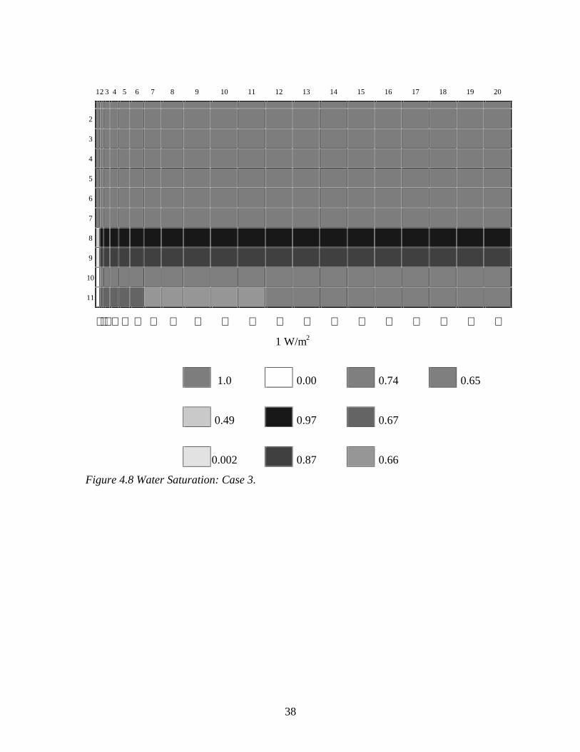
For all the cases, layers 1 to 7 were liquid-filled. For Case 1, it was observed that layers 8to 11 were filled up with a two-phase fluid (Fig. 4.6). Decreasing the maximum capillarypressure in the fracture blocks from 200 kPa to 100 kPa resulted in the lowermost block infracture being completely filled with steam (Fig. 4.7). Lowering the maximum capillarypressure in the fracture blocks resulted in having the two blocks which are steam-filled(Fig. 4.8).

12 3 4 5 6 7 8 9 10 11 12 13 14 15 16 17 18 19 20

2

3

4

5

6

7

8

9

10

11

⇑⇑⇑⇑ ⇑ ⇑ ⇑ ⇑ ⇑ ⇑ ⇑ ⇑ ⇑ ⇑ ⇑ ⇑ ⇑ ⇑ ⇑ ⇑

1 W/m2

1.0 0.4 0.68

0.81 0.33 0.56

0.52 0.95 0.51

Figure 4.6 Water Saturation: Case 1.

37

12 3 4 5 6 7 8 9 10 11 12 13 14 15 16 17 18 19 20

2

3

4

5

6

7

8

9

10

11

⇑⇑⇑⇑ ⇑ ⇑ ⇑ ⇑ ⇑ ⇑ ⇑ ⇑ ⇑ ⇑ ⇑ ⇑ ⇑ ⇑ ⇑ ⇑

1 W/m2

1.0 0.01 0.96 0.66

0.65 0.00 0.75 0.61

0.18 0.95 0.76

Figure 4.7 Water Saturation: Case 2.

For the case where the capillary pressure in the fracture is zero, it was observed that threeof the blocks in the fracture became fully filled with steam (Fig. 4.9). For the base casewhere no capillary pressures were assigned to both the matrix and fracture blocks, thefracture was observed to be liquid-filled.

Capillary forces do influence the fluid flow between the fracture and the adjacent matrix.In Case 1, the capillary pressure in the fracture was high. Therefore, more fluid is suckedinto the crevices, which explains the existence of the two-phase liquid in the fracture. Aswe lower the maximum capillary pressure, less of the liquid is retained. This accounts forthe decrease in water saturation and the development of steam-filled fracture blocks.

38

12 3 4 5 6 7 8 9 10 11 12 13 14 15 16 17 18 19 20

2

3

4

5

6

7

8

9

10

11

⇑⇑⇑⇑ ⇑ ⇑ ⇑ ⇑ ⇑ ⇑ ⇑ ⇑ ⇑ ⇑ ⇑ ⇑ ⇑ ⇑ ⇑ ⇑

1 W/m2

1.0 0.00 0.74 0.65

0.49 0.97 0.67

0.002 0.87 0.66

Figure 4.8 Water Saturation: Case 3.

39

12 3 4 5 6 7 8 9 10 11 12 13 14 15 16 17 18 19 20

2

3

4

5

6

7

8

9

10

11

⇑⇑⇑⇑ ⇑ ⇑ ⇑ ⇑ ⇑ ⇑ ⇑ ⇑ ⇑ ⇑ ⇑ ⇑ ⇑ ⇑ ⇑ ⇑

1 W/m2

1.0 0.94 0.70

0.256 0.81 0.69

0.00 0.71

Figure 4.9 Water Saturation: Case 4.

4.3 SUMMARY

The fracture was modeled by thin blocks which were given a high porosity value and arelatively high permeability. A nine-point differencing scheme was used when numericalsimulations were carried out with TETRAD in order to minimize the grid orientationeffects. To investigate the effect of capillary forces, several capillary pressure curves wereassigned to the matrix and fracture blocks. With the two-dimensional model, we were ableto observe the effects of capillary forces on the state of the system. These results arepreliminary. A more detailed observation on the effects of capillary pressures on fluid flowwill be conducted in the next quarter.

40

5 MODELING OF GEOTHERMAL RESERVOIRS CONSTRAINEDTO INJECTION RETURN DATA

This project is being conducted by Research Assistant Ma. Michelle Sullera and Prof.Roland Horne . It aims to deduce the injection return mechanisms and flow paths fromcorrelations between chloride concentration at producing wells and operating parameters(flow rate and injection chloride) at injection wells.

5.1 BACKGROUND

Traditionally, tracer tests are used to establish the degree of connectivity between wells.However, for wells which are only weakly connected these tests may need to beconducted over long periods of time using huge amounts of tracer of sufficient stability toobtain meaningful data. In such cases tracer tests would be too costly and impractical.

On the other hand, there are substances naturally occurring in the reservoir which behavelike tracers. One such substance is chloride. In Palinpinon, a geothermal field in thePhilippines, some injectors and producers are sufficiently strongly connected that changesin injection rates result in corresponding increases or decreases in produced chlorideconcentrations. The magnitude of the changes in chloride concentration reflect the degreeof communication between the wells. Moreover, chloride is stable, conservative; and free.We can therefore extract the same, if not more, information from chloride data as wecould from traditional tracer tests, at lower cost. This is just what this project proposes todo.

Specifically, this project aims to identify possible flow paths and injection returnmechanisms from analysis of chloride production data and injection data in producinggeothermal fields.

5.2 MODELING APPROACH

Following is a very general approach to the problem: First, seek a correlation betweenchloride concentrations in production wells and injection rates. Second, deducemechanisms, consistent with the previously obtained correlation, by which injectate returnsto the reservoir and is reproduced. Then, verify the accuracy of these mechanisms byincorporating them into a simulation model of the reservoir and generating historymatches.

As the first step of this work, during the current quarter, production and injection datafrom Palinpinon-I geothermal field were analyzed. To quantify the degree of connectivity

41

between producers and injectors in the said field, it was initially postulated that there is alinear relationship between produced chloride concentration and injection rates:

ClP = a0 + a1QI1 + a2QI2 + a3QI3 + ... ... + anQIn CORRELATION 1 (5.1)

where ClP = chloride concentration in production well, P

QIn = mass flow rate to injection well, In

an = linear coefficient of well In

a0 = a constant associated with local chloride concentration

A high value of an indicates a strong connection between producer P and injector In.

Recognizing that apart from its dependence on injection rates chloride concentration alsohas a natural tendency to increase with time as the reservoir is produced, a secondcorrelation with an additional linear term in time was proposed:

ClP = a0 + a1QI1 + a2QI2 + a3QI3 + ... ... + anQIn + ct CORRELATION 2 (5.2)

5.3 RESULTS AND DISCUSSION

Using production data from Palinpinon, values of the linear coefficients in Eqn. (5.1) and(5.2) were calculated and predicted values of chloride plotted against actual data. Resultsfor two typical production wells are shown in Figs. (5.1) and (5.2).

One interesting result is that some of the coefficients had negative calculated values. Thisimplies that the operation of injection wells corresponding to those negative coefficientscan actually lessen the percentage of injectate being produced at some locations. Oneplausible physical explanation is that the injectors with negative coefficients could bediverting the flow from the other injectors away from the production well.

Comparing Figures (5.1) and (5.2), we note that correlation 2 fits the data better thancorrelation 1. To test how well correlation 2 can predict chloride concentrations, only theportion of the data set spanning 1983 and 1986 was used to calculate the coefficients, thenchloride concentrations for the succeeding two years were predicted. Figure 5.3 showsthat correlation 2 (Eqn. 5.2) matches the portion of the data used for calculating thecoefficients fairly well but overpredicts and underpredicts the chloride concentration forthe next two years for wells P1 and P2, respectively.

42

Well P1

0

2000

4000

6000

8000

10000

12000

1983 1984 1985 1986 1987 1988 1989

Ch

lori

de,

pp

m

Data

Correlation 1

Well P2

0

1000

2000

3000

4000

5000

6000

1983 1984 1985 1986 1987 1988 1989

Ch

lori

de,

pp

m

Data

Correlation 1

Fig. 5.1 Actual vs. predicted chloride concentration using Eqn. 5.1

Well P1

0

1000

2000

3000

4000

5000

6000

7000

8000

9000

10000

1983 1984 1985 1986 1987 1988 1989

Ch

lori

de,

pp

m

Data

Correlation 2

Well P2

0

1000

2000

3000

4000

5000

6000

1983 1984 1985 1986 1987 1988 1989

Ch

lori

de

, pp

m

Data

Correlation 2

Fig. 5.2 Actual vs. predicted chloride concentration using Eqn. 5.2

Well P1

0

2000

4000

6000

8000

10000

12000

1983 1984 1985 1986 1987 1988 1989

Ch

lori

de,

pp

m

Data

Correlation 2 (Set B)

Well P2

0

1000

2000

3000

4000

5000

6000

1983 1984 1985 1986 1987 1988 1989

Ch

lori

de,

ppm

Data

Correlation 2 (Set B)

Fig. 5.3 Actual vs. predicted chloride concentration using Eqn. 5.2, 1983-1986 data

43

5.4 FUTURE PLANS

Correlation 2 gave a good match over the range of data where the coefficients werecalculated from but displayed poor predicting capability. The next step will be to see if theincorporation of additional data could improve the predictive capacity. Also, a nonlinearmodel of chloride concentration with time will be incorporated to account for the fact thatchloride does not increase indefinitely with time. After arriving at a satisfactorycorrelation, we plan to incorporate it with the reservoir model and generate productionhistory matches to test its accuracy.

44

6 EVALUATION OF SUB-SCALE HETEROGENEITIES INGEOTHERMAL ROCKS

This project is being conducted by Research Assistant Meiqing He, Dr. Cengiz Satik andProfessor Roland Horne. The aim of this project is to identify and characterize fracturesexisting in geothermal rocks by using X-ray computer tomography (CT) equipment. Thedescription of water or steam’s propagation in heterogeneous porous media is currentlypoorly understood, and in particular the effect of fractures on water or steam distribution,especially under geothermal reservoir condition, is still unknown. There are severalconcerns related to the necessity of evaluating of heterogeneity of rocks. From previousexperiments it has been found that adsorption and the distribution of water or steam in anetwork consisting of small fractures are not negligible in mass transfer processes, even infractures with aperture of order 1µm.This research will attempt to elucidate the factorsgoverning liquid and vapor propagation in heterogeneous porous media. Particularemphasis is given to the characterization of rock heterogeneity by using X-ray CT imagingtechnique in order to obtain a complete understanding of water and steam saturation inheterogeneous and fractured rocks under geothermal reservoir conditions.

The general goal is to advance the understanding of heterogeneity and evaluate its impacton mass transfer. The specific goals are as follows:

• Investigate X-ray CT imaging techniques to improve precision in the measurements ofsaturation and porosity of fractured and very heterogeneous rocks.

• Characterize the fracture geometry of rock samples from the Geysers geothermal fieldusing the X-ray CT scanner.

• Extract information about pore space from X-ray attenuation coefficients whichdepend on the density of material and the energy level used during the experiments. Inthis regard, we will experiment with multiple energy scans for the first time.

6.1 X-RAY CT TECHNIQUE AND APPLICATION

X-ray computerized tomography (CT) is a non-destructive measurement technology thatcan produce a higher resolution internal image of an object than conventional X-raymethods. It has been commonly applied in the study of rock properties. Unit elements inthe generated two-dimensional image matrix generated by the X-ray CT scanner arereferred to as CT numbers. Each CT number corresponds to the average attenuationcoefficient (µvoxel ) within a voxel. The object is divided into cubic voxels which can bethought of as pixels with a thickness. The thickness of a voxel is equal to the slicethickness (X-ray beam thickness) and the square dimension of a voxel is defined by thelength of the detectors divided by the dimension of the image matrix which is a result ofthe sampling rate.

45

Prior to display of a CT image, it is conventional in the medical field to normalize the X-ray attenuation data to water in the following fashion:

CT voxel water

water

=−2048( )µ µ

µ (6.1)

where µ is the X-ray attenuation coefficient and CT is the CT number, the unit of which iscalled a Hounsfield. This equation results in CT numbers of -1024 Hounsfield for air, 0Hounsfield for water, and 1024 Hounsfield for bone.

The relationship between detected intensity Id and incident intensity I0 can be expressedas

( ) ( )[ ]I x y I x y z dz dd ( , ) exp , , ,= −∫ ∫0 ε µ ε ε (6.2)

where ( )I0 ε is the incident X-ray beam intensity as a function of the energy per photon εand µ(x, y, z, ε) is the linear attenuation coefficient at each region of the object. The µ ofall materials depends on the photon energy of the beam and the atomic number of theelements in the material (Johns and Cunnigham, 1974). X-ray energy is quantumized intophotons. The decrease in the intensity of the X-ray beam after traversing an object isdescribed by the photon absorption or scattering. Attenuation mechanisms are composedof coherent or Rayleigh scatter, photoelectric absorption, and Compton scatter in thediagnostic range, below 200 kev (kilo electron volts).

µ µ µ µ= + +R P C (6.3)

Photoelectric absorption dominates in materials with higher atomic-number material. Theattenuation coefficient undergoes a sharp increase in the energy region corresponding tothe K shell. For high atomic-number material, the K absorption edge occurs within thespectrum of interest. On the other hand, Compton scatter dominates in low atomic-number material, such as water and soft tissue (Macovski, 1983). Regarding the materialsof geothermal interest, namely water, steam and rock, only the Compton effect andphotoelectric adsorption are expected to be dominant while coherent scatter only happenswhen the X-ray energy is of the order of a few kev which is not within the energy levelrange of our experiment. The Compton attenuation contribution µC to the total attenuationis dependent on the energy µ, but independent of atomic number. The photoelectriccomponent is dependent on both atomic number and energy level. In order to inspect theappropriateness of the CT numbers generated by our equipment, we wrote code to checkthe value by tracing the saturation calculation process. Some CT numbers were found tobe out of reasonable range under some experimental conditions. We refer to these as

46

“noise”. Instead of simply disregarding those numbers we are trying to uncover thepossible mechanisms of any errors in the imaging system and to find an approach tocorrect for these effects.

6.2 PLAN FOR FUTURE WORK

Since our CT scanner system was originally manufactured for medical uses, there are somedata processing algorithms which might not be optimal for our study object (core). Wewill seek more appropriate algorithms than the one chosen currently to correct beamhardening effect when scanning human bone. Our approach to determine heterogeneitiesin the cores as well as their saturation distributions by running multilevel energy scans willbe established on the relationship between the material’s attenuation coefficients and theenergy level of the CT scan (Huang, Ringrose and Sorbie, 1996)

47

7 STUDY OF HEAT TRANSFER AND BOILING IN A FRACTURE

This new research initiative has been conducted by Robert DuTeaux under the guidance ofDr. Shaun Fitzgerald and Dr. Cengiz Satik. The project was developed to improve ourunderstanding of heat transfer and boiling in a discrete fracture by the concomitantdevelopment of an experimental apparatus and a numerical model.

7.1 SUMMARY

The initial work on this project has involved the conception and design of an experimentalapparatus. A review of literature provided a moderate background of information that willbe relevant to the verification of the apparatus with single phase flow and heat transfer,however, only limited experimental or numerical work with liquid injection and boiling in adiscrete fracture has been conducted previously. The ultimate objectives of this researchwill be to analyze the temperature gradients adjacent to a fracture caused by liquidinjection and boiling in that fracture, and to understand the movement of the liquid-vaporinterface as heat is depleted from the solid medium by conduction to the fracture andconvection in the direction of flow with the fluid. An explanation of the apparatus designwith a brief projection of the future work follows.

7.2 EXPERIMENTAL APPARATUS DESIGN

The physical properties of the materials used to model fluid flow, heat transfer, and phasechange in a discrete fracture have been selected to be similar to the physical properties ofrock, and water was selected as working fluid in the design. It was agreed that thecylindrical annulus formed between two large diameter concentric glass tubes bestsimulated a parallel plate fracture geometry and removed the end-effects of simply usingtwo flat plates. Figure 7.1 illustrates the design that was developed.

The diameter of the core in Figure 7.1 is slightly more than five inches and the height ofthe assembly is eighteen inches. The core of the apparatus contains thermocouplesembedded in sand (or another medium) completely enclosed in glass so that fluid may onlyflow in the annulus formed by the two concentric glass tubes. The annulus between theglass tubes is approximately two millimeters wide. Outside the larger glass tube is a thirdconcentric acrylic tube with two functions. It allows an insulating vacuum around theapparatus and also serves to contain the glass for safety. At the end of this first quarter ofthis research the materials needed for the assembly had been acquired and the apparatuswas almost ready for construction.

48

Figure 7.1 The experimental apparatus design.

7.3 NUMERICAL MODELING

This experimental assembly was intended not only for analysis by empirical observation,but also was intended to provide data for comparison to a numerical model yet to bedeveloped. For the case where heat is transferred radially and axially to the surface of acylinder with a transient surface temperature distribution there is no exact analyticsolution. It was decided, therefore, to simulate this phenomenon numerically. Subsequentreports will document further progress towards this goal.

49

7.4 FUTURE PLAN

In the next quarter, the apparatus will initially be used to obtain data for single phase flowand heat transfer which will be used to evaluate the quality of the experimental design bycomparison to numerical simulation. Also, different materials will be used to make thecore of the assembly and different thermocouple patterns will be tried. After sufficienttrials the apparatus will be used to observe boiling by placing a heated core into theassembly and injecting saturated water into the base and up the annulus. The flow will becontrolled at various constant flow rates, and also under constant pressure conditions withan atmospheric outlet pressure. Our future plans also include encoding a two-phasenumerical simulation.

50

8 PRODUCTIVITY VARIATION DUE TO PHASE CHANGE

This research project is being conducted by Research Assistant, Marilou Guerrero, Prof.Shaun Fitzgerald, and Prof. Roland Horne. The purpose of this study is to improve ourunderstanding of productivity index variation due to phase change in geothermalreservoirs by analytical and numerical methods.

8.1 INTRODUCTION

The calculation of productivity index in present reservoir simulators is basically only forsingle-phase flow. In geothermal systems, however, boiling occurs as pressure drops (i.e.in the case of a water-dominated reservoir). When this happens, the productivity indexmay no longer be a function of wellbore geometry and permeability. It can vary with time,as geothermal fluids are withdrawn from the reservoir. Thus, it is the objective of thisresearch project to investigate the appropriateness of the commonly used pressure dropequations for two-phase flow into geothermal wells. This will impact economic value ofgeothermal projects, and therefore is an important aspect of project evaluation.

This report will describe a brief literature review, derivation of governing equations forphysical processes in geothermal systems, and discussion of future work.

8.2 REVIEW OF RELATED LITERATURE

In reservoir simulation, pressure at a grid point is taken as the average of the pressure ofthe block surrounding the grid point. However, for large grid block sizes, a well locatedin this block cannot use the calculated pressure of the block. One of the techniquesdeveloped to solve this problem is by using analytical well models.

Schwabe and Brand (1967) developed their analytical model for single-phase flow fromthe radial form of Darcy’s law. In the absence of skin effect, it is simplified to

q = 2πkh (po -pwf) / [µ ln(∆x/rw)] (8.1)

where k is the permeability, h is the reservoir thickness, po is the simulator well blockpressure, pwf is the flowing wellbore pressure, µ is the fluid viscosity, ∆x is the grid blockspacing, and rw is the wellbore radius. For large grid blocks, van Poolen et al (1968)suggested that

q = 2πkh (po -pwf) / [µ ln (∆x/ (rw √π)) - ½] (8.2)

The basic assumption here is that well block pressure is the areal average pressure.

A productivity index, PI, can be defined as

q = PI (po - pwf)/µ (8.3)

51

Using the expression for q in Equation (8.2),

PI = 2πkh / [ln ((√∆x ∆y/ π)/rw) - ½] (8.4)

This expression is similar to the productivity index defined by Coats et al (1974).

In 1978, Peaceman showed that the well block pressure is equal to the actual flowingpressure at a radius, ro, for a square grid block. This is expressed as

ro = 0.2 ∆x (8.5)

Defining ro as the equivalent wellbore radius, or that radius at which the steady-stateflowing pressure of the actual well equals the numerically calculated pressure for the wellblock,

q = 2πkh (po -pwf) / [µ ln(ro/rw)] (8.6)

Comparing Equations (8.2) and (8.6) gives

ro = 0.342 ∆x (8.7)

This result is based on the assumption that the well block pressure is equal to the arealpressure; and it contradicts Peaceman’s conclusion that ro = 0.2 ∆x.

Furthermore, Peaceman (1982 1983) showed that for a uniform rectangular grid

ro = 0.14 √(∆x2 + ∆y2) (8.8)

for single-phase flow.

8.3 GOVERNING EQUATIONS

The general governing equations presented here consist of mass and thermal energybalances for the steam and water phases present in a geothermal system. Assumingsteady-state conditions, these balance equations are reduced to two nonlinear partialdifferential equations:

[-M/2πdk][1/r (∂p/∂r)]= ρLSn/µL + ρV(1-S)n/µV (8.9)

[-M/2πdk][1/r (∂p/∂r)]=1/CLTH { ρLSnCL/µL [T* + (∂T/∂p)sat(p-p*)] + ρV(1-S)n/µV} (8.10)

where M is the total mass flux, d is the reservoir thickness, k is the formation permeability,r is the distance from a constant pressure boundary to the wellbore, p is the reservoirpressure, C is the specific heat, TH is the temperature of the single-phase water comingfrom the boundary, ρ is the fluid density, µ is the fluid viscosity, T* is the reservoirtemperature at a reference point, p* is the reservoir pressure at a reference point, and S isthe water saturation. Variables with subscript “L” refers to the water phase, while thosewith subscript “V” refers to the steam phase.

52

8.4 FUTURE WORK

The ultimate goal of this project is to formulate an equation for productivity index thattakes into account boiling or phase change in geothermal reservoirs. To verify thisequation, the reservoir simulator TOUGH2 will be used. A section code will be written toadjust the productivity calculation in the simulator.

REFERENCES

1. Fitzgerald, S.D. and Woods, A.W. 1994 The instability of a vaporization front in hotporous rock. Nature 367, 450-453.

2. Hornbrook, J. W. and Faulder, D. D. (1993) Parametric analysis of factors affectinginjection and production in geothermal reservoirs. Proc. Stanford Geoth. Workshop18, 53-60.

3. Huang,Y., Ringrose, P.S. and Sorbie, K.S., “X-ray Imaging of Waterflood FluidSaturation in Heterogeneous Rock Slabs”, SPE 30000, presented at the 1996 SPEAnnual Meeting, Denver, CO, pp. 483-495.

4. Johns, J.R., Steude, J.S., Castanier, L.M. and Roberts, P.V., 1993, “NondestructiveMeasurements Of Fracture Aperture In Crystalline Rock Core Using X-Ray ComputedTomography”, J. Geophys. Res., 98(B2), 1889-1900

5. Johns, R.A., “Diffusion and Dispersion of Solute in a Variable Aperture Fracture”,1991, PhD dissertation, Stanford University

6. Macovski, A. (1983), “Medical Imaging System”, Prentice Hall

7. Pruess, K. (1991) Grid orientation and capillary pressure effects on the simulation ofwater injection into depleted vapor zones. Geothermics 20 (No. 5/6), 257-277.

8. Pruess, K. 1991 TOUGH User’s Guide. Earth Sci. Div., Report LBL-20700,Lawrence Berkeley Laboratory.

9. Pruess, K., Calore, C., Celati, R. and Wu, Y.S. 1987 An analytical solution for heattransfer at a boiling front moving through a porous medium. Int. J. Heat MassTransfer 30(12), 2595-2602.

10. Satik, C., 1994, “Studies In Vapor-Liquid Flow In Porous Media”, Ph.D. Thesis,University of Southern California, Los Angeles, CA

11. Satik, C., Ambusso, W., Castanier, L.M. and Horne, R.N., 1995, “A PreliminaryStudy of Relative Permeability In Geothermal Rocks”, Trans. GRC, 19, 539

12. Satik, C. and Yortsos, Y.C., 1996, “A Pore Network Study Of Bubble Growth InPorous Media Driven By Heat Transfer”, J. Heat Transfer, 118

53

13. Satik, C. and Horne, R.N., 1996, “An Experimental Study of Boiling In PorousMedia”, Trans. GRC,20, 839

14. Weast, R.C. 1972 Handbook of Chemistry and Physics. Chemical Rubber Co.

15. Woods, A.W. and Fitzgerald, S.D. 1993 The vaporization of a liquid front movingthrough a hot porous rock. J. Fluid Mech. 251, 563-579.

16. Woods, A.W. and Fitzgerald, S.D. 1996 The effects of heat conduction on thevaporization of liquid invading superheated permeable rock. Proc. StanfordGeothermal Reservoir Engineering Workshop 21, 421-425.

17. Woods, A.W. and Fitzgerald, S.D. 1997 The vaporization of a liquid front movingslowly through a hot porous rock. Part II J. Fluid Mech. in press