stability of the determination of a time-dependent … · · 2017-01-24stability of the...
TRANSCRIPT

Stability of the determination of a time-dependent
coefficient in parabolic equations
Mourad Choulli, Yavar Kian
To cite this version:
Mourad Choulli, Yavar Kian. Stability of the determination of a time-dependent coefficient inparabolic equations. Mathematical Control and Related Fields, AIMS, 2013, 3 (2), pp.143-160.<10.3934/mcrf.2013.3.143>. <hal-00673690v2>
HAL Id: hal-00673690
https://hal.archives-ouvertes.fr/hal-00673690v2
Submitted on 28 Feb 2012
HAL is a multi-disciplinary open accessarchive for the deposit and dissemination of sci-entific research documents, whether they are pub-lished or not. The documents may come fromteaching and research institutions in France orabroad, or from public or private research centers.
L’archive ouverte pluridisciplinaire HAL, estdestinee au depot et a la diffusion de documentsscientifiques de niveau recherche, publies ou non,emanant des etablissements d’enseignement et derecherche francais ou etrangers, des laboratoirespublics ou prives.

STABILITY OF THE DETERMINATION OF A TIME-DEPENDENT COEFFICIENT
IN PARABOLIC EQUATIONS
MOURAD CHOULLI AND YAVAR KIAN
Abstract. We establish a Lipschitz stability estimate for the inverse problem consisting in the determi-nation of the coecient σ(t), appearing in a Dirichlet initial-boundary value problem for the parabolicequation ∂tu − ∆xu + σ(t)f(x)u = 0, from Neumann boundary data. We extend this result to the sameinverse problem when the previous linear parabolic equation is changed to the semi-linear parabolic equation∂tu− ∆xu = F (t, x, σ(t), u(x, t)).
Key words : parabolic equation, semi-linear parabolic equation, inverse problem, determination of time-depend coecient, stability estimate.
AMS subject classications : 35R30.
Contents
1. Introduction 12. Time-dierentiability of potential-type functions 43. Proof of Theorems 1 and 2 12References 14
1. Introduction
Throughout this paper, we assume that Ω is a C3 bounded domain of Rn with n > 2. Let T > 0 and set
Q = Ω× (0, T ), Γ = ∂Ω, Σ = Γ× (0, T ).
We consider the following initial-boundary value problem∂tu−∆xu+ σ(t)f(x)u = 0, (x, t) ∈ Q,u(x, 0) = h(x), x ∈ Ω,
u(x, t) = g(x, t), (x, t) ∈ Σ.
(1.1)
We introduce the following assumptions :
(H1) f ∈ C2(Ω), h ∈ C2,α(Ω), g ∈ C2+α,1+α2 (Σ), for some 0 < α < 1, and satisfy the compatibility
condition∂tg(x, 0)−∆xh(x) + σ(0)f(x)h(x) = 0, x ∈ Γ.
(H2) There exists x0 ∈ Γ such that
inft∈[0,T ]
|g(x0, t)f(x0)| > 0.
Under assumption (H1), it is well known that, for σ ∈ C1[0, T ], the initial-boundary value problem (1.1)admits a unique solution u = u(σ) ∈ C2+α,1+α
2 (Q) (see Theorem 5.2 of [LSU]). Moreover, given M > 0,there exists a constant C > 0 depending only on data (that is Ω, T , f , g and h) such that ‖σ‖W 1,∞(0,T ) 6Mimplies
‖u(σ)‖C2+α,1+α/2(Q) 6 C. (1.2)
1

2 MOURAD CHOULLI AND YAVAR KIAN
In the present paper we are concerned with the inverse problem consisting in the determination of thetime dependent coecient σ(t) from Neumann boundary data ∂νu(σ) on Σ, where ∂ν is the derivative in thedirection of the unit outward normal vector to Γ.
We prove the following theorem, where B(M) is the ball of C1[0, T ] centered at 0 and with radiusM > 0.
Theorem 1. Assume that (H1) and (H2) are fullled. For i = 1, 2, let σi ∈ B(M) and ui = u(σi). Thenthere exists a constant C > 0, depending only on data, such that
‖σ2 − σ1‖L∞(0,T ) 6 C ‖∂t∂νu2 − ∂t∂νu1‖L∞(Σ) . (1.3)
Following [COY], it is quite natural to extend Theorem 1 when the linear parabolic equation is changedto a semi-linear parabolic equation. To this end, introduce the following semi-linear initial-boundary valueproblem :
∂tu−∆xu = F (x, t, σ(t), u(x, t)), (x, t) ∈ Q,u(x, 0) = h(x), x ∈ Ω,
u(x, t) = g(x, t), (x, t) ∈ Σ
(1.4)
and consider the following assumptions
(H3) h ∈ C2,α(Ω), g ∈ C2+α,1+α2 (Σ), for some 0 < α < 1, and satisfy the compatibility condition
∂tg(x, 0)−∆xh(x) = F (0, x, σ(0), h(x)), x ∈ Γ.
(H4) F ∈ C1(Ωx × Rt × Rσ × Ru) is such that ∂uF and ∂σF are C1, F and ∂σF are C2 with respect to xand u.
(H5) There exist M > 0 and x0 ∈ Γ such that
inft∈[0,T ],σ∈[−M,M ]
|∂σF (x0, t, σ, g(x0, t))| > 0.
(H6) There exist two non negative constants c and d such that
uF (x, t, σ(t), u) 6 cu2 + d, t ∈ [0, T ], x ∈ Ω, u ∈ R.
Under the above mentioned conditions, for any σ ∈ C1[0, T ], the initial-boundary value problem (1.4)admits a unique solution u = u(σ) ∈ C2+α,1+α
2 (Q) (see Theorem 6.1 in [LSU]) and, givenM > 0, there existsa constant C > 0 depending only on data (that is Ω, T , F , g and h) such that ‖σ‖W 1,∞(0,T ) 6M implies
‖u(σ)‖C2+α,1+α/2(Q) 6 C. (1.5)
We have the following extension of Theorem 1.
Theorem 2. Assume that (H3), (H4), (H5) and (H6) are fullled. For i = 1, 2, let σi ∈ B(M) andui = u(σi). Then there exists a constant C > 0, depending only on data, such that
‖σ2 − σ1‖L∞(0,T ) 6 C ‖∂t∂νu2 − ∂t∂νu1‖L∞(Σ) . (1.6)
Remark 1. Let us observe that we can generalize the results in Theorems 1 and 2 as follows:
i) In (1.1), we can replace σ(t)f(x) by∑pk=1 σk(t)fk(x), where fk, 1 6 k 6 p, are known. Assume that
(H1) is satised, with f = fk for each k, where the compatibility condition is changed to
∂tg(x, 0)−∆xh(x) +
p∑k=1
σk(0)fk(x)h(x) = 0, x ∈ Γ.
Therefore, to each (σ1, . . . , σp) ∈ C[0, T ]p corresponds a unique solution u = u(σ1, . . . , σp) ∈ C2+α,1+α/2(Q)and max‖σk‖W 1,∞(0,T ); 1 6 k 6 p 6M implies
‖u(σ1, . . . , σp)‖C2+α,1+α/2(Q) 6 C,
for some positive constant C depending only on data.

STABILITY OF THE DETERMINATION OF A TIME-DEPENDENT COEFFICIENT IN PARABOLIC EQUATIONS 3
Following the proof of Theorem 1, we prove that, under the following conditions : there exist x1, . . . , xp ∈Γ such that the matrix M(t) = (fk(xl)g(xl, t)) is invertible for any t ∈ [0, T ],
max16k6p
‖σ1k − σ2
k‖L∞(0,T ) 6 C ‖∂t∂νu2 − ∂t∂νu1‖L∞(Σ) ,
if σjk ∈ B(M), 1 6 k 6 p and j = 1, 2. Here C is a constant that can depend only on data and uj =
u(σj1, . . . , σjp), j = 1, 2.
ii) We can replace the semi-linear parabolic equation in (1.4) by a semi-linear integro-dierential equa-tion. In other words, F can be changed to
F1(x, t, σ(t), u(x, t)) +
∫ t
0
F2(x, s, σ(t− s), u(x, s))ds.
Under appropriate assumptions on F1 and F2, one can establish that Theorem 2 is still valid in the presentcase.
ii) Both in (1.1) and (1.4), the Laplace operator can be replaced by a second order elliptic operator indivergence form :
E = ∇ ·A(x)∇+B(x) · ∇,where A(x) = (aij(x)) is a symmetric matrix with coecients in C1+α(Ω), B(x) = (bi(x)) is a vector with
components in Cα(Ω) and the following ellipticity condition holds
A(x)ξ · ξ > λ |ξ|2 , ξ ∈ Rn, x ∈ Ω.
Actually, the normal derivative associated to E is the boundary operator ∂νE = ν(x) ·A(x)∇.
To our knowledge, there are only few results concerning the determination of a time-dependent coecientin an initial-boundary value problem for a parabolic equation from a single measurement. The determinationof a source term of the form f(t)χD(x), where χD the characteristic function of the known subdomain D, wasconsidered by J. R. Canon and S. P. Esteva. They established in [CE86-1] a logarithmic stability estimatein 1D case in a half line when the overdetermined data is the trace at the end point. A similar inverseproblem problem in 3D case was studied by these authors in [CE86-2], where they obtained a Lipschitzstability estimate in weighted spaces of continuous functions. The case of a non local measurement wasconsidered by J. R. Canon and Y. Lin in [CL88] and [CL90], where they proved existence and uniquenessfor both quasilinear and semi-linear parabolic equations. The determination of a time dependent coecientin an abstract integrodierential equation was studied by the rst author in [Ch91-1]. He proved existence,uniqueness and Lipschitz stability estimate, extending earlier results by [Ch91-2], [LS87], [LS88], [PO85-1]and [PO85-2]. In [CY06], the rst author and M. Yamamoto obtained a stability result, in a restrictedclass, for the inverse problem of determining a source term f(x, t), appearing in a Dirichlet initial-boundaryvalue problem for the heat equation, from Neumann boundary data. In a recent work, the rst authorand M. Yamamoto [CY11] considered the inverse problem of nding a control parameter p(t) that reach adesired temperature h(t) along a curve γ(t) for a parabolic semi-linear equation with homogeneous Neumannboundary data and they established existence, uniqueness as well as Lipschitz stability. Using geometric opticsolutions, the rst author [Ch09] proved uniqueness as well as stability for the inverse problem of determininga general time dependent coecient of order zero for parabolic equations from Dirichlet to Neumann map. In[E07] and [E08], G. Eskin considered the same inverse problem for hyperbolic and the Schrödinger equationswith time-dependent electric and magnetic potential and he established uniqueness by gauge invariance.Recently, R. Salazar [Sa] extended the result of [E07] and obtained a stability result for compactly supportedcoecients.
We would like to mention that the determination of space dependent coecient f(x), in the sourceterm σ(t)f(x), from Neumann boundary data was already considered by the rst author and M. Yamamoto[CY06]. But, it seems that our paper is the rst work where one treats the determination of a time dependentcoecient, appearing in a parabolic initial-boundary value problem, from Neumann boundary data.

4 MOURAD CHOULLI AND YAVAR KIAN
This paper is organized as follows. In section 2 we come back to the construction of the Neumannfundamental solution by [It] and establish time-dierentiability of some potential-type functions, necessaryfor proving Theorems 1 and 2. Section 3 is devoted to the proof of Theorems 1 and 2.
2. Time-differentiability of potential-type functions
In this section, we establish time-dierentiability of some potential-type functions, needed in the proofof our stability estimates. In our analysis we follow the construction of the fundamental solution by S. Itô[It].
First of all, we recall the denition of fundamental solution associate to the heat equation plus a time-dependent coecient of order zero, in the case of Neumann boundary condition. Consider the initial-boundary value problem
∂tu = ∆xu+ q(x, t)u, (x, t) ∈ Ω× (s, t0),
limt→s
u(x, t) = u0(x), x ∈ Ω,
∂νu(x, t) = 0, (x, t) ∈ Γ× (s, t0).
(2.1)
Here s0 < t0 are xed, s ∈ (s0, t0), u0 and q(x, t) are continuous respectively in Ω and in Ω × [s, t0]. LetU(x, t; y, s) be a continuous function in the domain s0 < s < t < t0, x ∈ Ω, y ∈ Ω. We recall that U is thefundamental solution of (2.1) if for any u0 ∈ C(Ω),
u(x, t) =
∫Ω
U(x, t; y, s)u0(y)dy
is the solution of (2.1). We refer to [It] for the existence and uniqueness of this fundamental solution.
We start with time-dierentiability of volume potential-type functions1.
Lemma 1. Fix s ∈ (s0, t0). Let f ∈ C(Ω× [s, t0]) be C2 with respect to x, q ∈ C1(Ω× [s, t0]) and dene, for(x, t) ∈ Ω× (s, t0),
f1(x, t; τ) =
∫Ω
U(x, t; y, τ)f(y, τ)dy, t > τ > s.
Then, f1 admits a derivative with respect to t and
∂f1
∂t(x, t; τ) =
∫Ω
U(x, t; y, τ)(∆y + q(x, τ))f(y, τ)dy
+
∫ t
τ
∫Ω
∫Ω
U(x, t; z, τ ′)∂tq(z, τ′)U(z, τ ′; y, τ)f(y, τ)dzdydτ ′.
(2.2)
Moreover, F given by
F (x, t) =
∫ t
s
f1(x, t; τ)dτ, (x, t) ∈ Γ× (s0, t0),
possesses a derivative with respect to t,
∂F
∂t(x, t) = f(x, t) +
∫ t
s
∂f1
∂t(x, t; τ)dτ (2.3)
and ∣∣∣∣∫ t
s
∂f1
∂t(x, t; τ)dτ
∣∣∣∣ 6 C ∫ t
s
‖f(., τ)‖C2x(Ω) dτ. (2.4)
1Recall that if ϕ = ϕ(x, t) is a continuous function then the corresponding volume potential is given by
ψ(x, t) =
∫ t
s
∫ΩU(x, t; y, τ)ϕ(y, τ)dydτ.

STABILITY OF THE DETERMINATION OF A TIME-DEPENDENT COEFFICIENT IN PARABOLIC EQUATIONS 5
Proof. We have only to prove (2.2) and (2.4), because (2.3) follows immediately from (2.2).
Let then u0 ∈ C2(Ω) and consider the function
u(x, t) =
∫Ω
U(x, t; y, s)u0(y)dy, x ∈ Ω, s < t < t0.
We show that u admits a derivative with respect to t and
∂tu(x, t) = ∂t
(∫Ω
U(x, t; y, s)u0(y)dy
)=
∫Ω
U(x, t; y, s)(∆y + q(x, s))u0(y)dy
−∫ t
s
∫Ω
∫Ω
U(x, t; z, τ)qt(z, τ)U(z, τ ; y, s)u0(y)dzdydτ.
(2.5)
We need to consider rst the case u0 = w0 ∈ C∞(Ω). Set
w(x, t) =
∫Ω
U(x, t; z, s)w0(y)dy, x ∈ Ω, s < t < t0.
Clearly, w(x, t) is the solution of the following initial-boundary value problem∂tw −∆xw − q(x, t)w = 0, (x, t) ∈ Ω× (s, t0),
limt→s
w(x, t) = w0(x), x ∈ Ω,
∂νw(x, t) = 0, (x, t) ∈ Γ× (s, t0)
and w1 = ∂tw satises ∂tw1 −∆xw1 − q(x, t)w1 = −∂tqw, (x, t) ∈ Ω× (s, t0),
limt→s
w1(x, t) = (∆x + q(x, s))w0(x), x ∈ Ω,
∂νw1(x, t) = 0, (x, t) ∈ Γ× (s, t0).
Therefore, (2.5), with w in place of u, is a consequence of Theorem 9.1 of [It].
Next, let (wn0 )n be a sequence in C∞(Ω) converging to u0 in C2(Ω) and v(x, t) given by
v(x, t) =
∫Ω
U(x, t; y, s)(∆x + q(x, s))u0(y)dy
−∫ t
s
∫Ω
∫Ω
U(x, t; z, τ)∂tq(z, τ)U(z, τ ; y, s)u0(y)dzdydτ.
Consider (wn)n, the sequence of functions, dened by
wn(x, t) =
∫Ω
U(x, t; z, s)wn0 (y)dy.
We proved that, for any n ∈ N,
∂twn(x, t) =
∫Ω
U(x, t; y, s)(∆y + q(x, s))wn0 (y)dy
−∫ t
s
∫Ω
∫Ω
U(x, t; z, τ)∂tq(z, τ)U(z, τ ; y, s)wn0 (y)dzdydτ.
(2.6)
From the proof of Theorem 7.1 of [It],∫Ω
|U(x, t; y, s)| dy 6 CeC(t−s), (x, t) ∈ Ω× (s, t0). (2.7)
Therefore, we can pass to the limit, as n goes to innity, in (2.6). We deduce that ∂twn converges to v inC(Ω × [s, t0]). But, wn converges to u in C(Ω × [s, t0]). Hence u admits a derivative with respect to t and

6 MOURAD CHOULLI AND YAVAR KIAN
∂tu = v. That is we proved (2.5) and consequently (2.2) holds true. Finally, we note that (2.4) is deducedeasily from (2.7).
Next, we consider time-dierentiability a single layer potential-type function2.
Lemma 2. Fix s ∈ (s0, t0). Let f ∈ C(Γ × [s, t0]) be C1 with respect to t ∈ [s, t0] with f(x, s) = 0. Dene,for (x, t) ∈ Γ× (s, t0),
f1(x, t; τ) =
∫Γ
U(x, t; y, τ)f(y, τ)dσ(y), t > τ > s.
Then
F (x, t) =
∫ t
s
f1(x, t; τ)dτ
is well dened, admits a derivative with respect to t and we have∥∥∥∥∂F∂t∥∥∥∥L∞(Γ×(s,t0))
6 C ‖∂tf‖L∞(Γ×(s,t0)) . (2.8)
Contrary to Lemma 1, for Lemma 2 we cannot use directly the general properties of the fundamental so-lutions developed in [It]. We need to come back to the construction of the fundamental solution of (2.1) intro-duced by [It]. First, consider the heat equation ∂tu = ∆xu in the half space Ω1 = x = (x1, . . . , xn); x1 > 0in Rn with the boundary condition ∂x1
u = 0 on Γ1 = x = (0, x2, . . . , xn); (x2, . . . , xn) ∈ Rn−1. For anyy = (y1, y2, . . . , yn), we dene y by y = (−y1, y2, . . . , yn). Let
G(x, t) =1
(4πt)n2e−|x|2t
denotes the Gaussian kernel and set
G1(x, t; y) = G(x− y, t) +G(x− y, t).Then, the fundamental solution U0(x, t; y, s) of
∂tu = ∆xu, (x, t) ∈ Ω1 × (s, t0),
limt→s
u(x, t) = u0(x), x ∈ Ω1,
∂νu(x, t) = 0, (x, t) ∈ Γ1 × (s, t0)
(2.9)
is given byU0(x, t; y, s) = G1(x, t− s; y).
In order to construct the fundamental solution in the case of an arbitrary domain Ω, Itô introduced thefollowing local coordinate system around each point z ∈ Γ.
Lemma 3. (Lemma 6.1 and its corollary, Chapter 6 of [It]) For every point z ∈ Γ, there exist a coordinateneighborhood Wz of z and a coordinate system (x∗1, . . . , x
∗n) satisfying the following conditions:
1) the coordinate transformation between the coordinate system (x∗1, . . . , x∗n) and the original coordinate
system in Wz is of class C2 and the partial derivatives of the second order of the transformation functionsare Hölder continuous ;2) Γ ∩Wz is represented by the equation x∗1 = 0 and Ω ∩Wz is represented by x∗1 > 0 ;3) let L be the dieomorphism from Wz to L(Wz) dened by
L : Wz → L(Wz)
x 7→ (x∗1(x), . . . , x∗n(x)).
2The single-layer potential corresponding to a continuous function ϕ = ϕ(x, t) is given by
ψ(x, t) =
∫ t
s
∫ΓU(x, t; y, τ)ϕ(y, τ)dσ(y)dτ.

STABILITY OF THE DETERMINATION OF A TIME-DEPENDENT COEFFICIENT IN PARABOLIC EQUATIONS 7
Then, for any u ∈ C1(Ω) we have
∂νu(ξ) = −∂x1(u L−1)(x), ξ ∈ Γ ∩Wz and x = L(ξ).
From now on, for any z ∈ Γ, we view coordinate system (x∗1, . . . , x∗n) as a rectangular coordinate system.
Moreover, using the local coordinate system of Lemma 3, for any y = (y1, y2, . . . , yn) ∈ L(Wz), we deney = (−y1, y2, . . . , yn) and, without loss of generality, we assume that, for any y ∈ L(Wz), we have y ∈ L(Wz).For any interior point z of Ω, we x an arbitrary local coordinate system and a coordinate neighborhood Wz
contained in Ω. For any z ∈ Ω and δ > 0, we set W (z, δ) = x : |x− z|2 < δ and δz > 0 such that, for any
z ∈ Ω we have W (z, δz) ⊂Wz.
Recall the following partition of unity lemma.
Lemma 4. (Lemma 7.1, Chapter 7 of [It]) There exist a nite subset z1, . . . , zm of Ω and a nite sequenceof functions ω1, . . . , ωm with the following properties:1) supp ωl ⊂W (zl, δzl), l = 1, . . . ,m, and each ωl is of class C3 with respect to the local coordinates in Wzl ;
2) ωl(x)2; l = 1, . . . ,m forms a partition of unity in Ω ;3)∂νωl(ξ) = 0, l = 1, . . . ,m, ξ ∈ Γ.
Let z1, . . . , zm be the nite subset of Ω, introduced in the previous lemma. For any k ∈ 1, . . . ,m,let Lk denotes the dieomorphism from Wzk to Lk(Wzk) dened by
Lk : Wzk → Lk(Wzk)
x 7→ (x∗1(x), . . . , x∗n(x)),
where (x∗1, . . . , x∗n) is the local coordinate system of Lemma 3 dened in Wzk . For any k ∈ 1, . . . ,m, the
dierential operator∂t −∆x − q(x, t)
becomes, in terms of local coordinate system x∗ = (x∗1, . . . , x∗n),
Lkt,x∗ = ∂t −1√
ak(x∗)
n∑i,j=1
∂x∗i
(√ak(x∗)aijk (x∗)∂x∗j ·
)− qk(x∗, t)
in Lk(Wzk) × (s0, t0). Here qk(x∗, t) is Hölder continuous on Lk(Wzk) × (s0, t0) and (aij(x∗)) is the con-travariant tensor of degree 2 dened by(
aijk (x∗))
=(JLk(L−1
k (x∗)))T (
JLk(L−1k (x∗))
),
with
JLk(x) =
(∂x∗j (x)
∂xi
).
According to the construction of [It] given in Chapter 6 (see pages 42 to 45 of [It]),(aijk (x∗)
)is of class
C2 in Lk(Ω ∩ Wzk) and it is a positive denite symmetric matrix at every point x∗ ∈ Lk(Wzk). We set
(akij(x∗)) = (aijk (x∗))−1 and ak(x∗) = det(ak
ij(x∗)). Consider the volume element dx∗ =
√ak(x∗)dx∗1 . . . dx
∗n
on Lk(Wzk) and dx′ =√a(0, x′)dx∗2 . . . dx
∗n on Lk(Wzk ∩ Γ) with x′ = (x∗2, . . . , x
∗n). Note that, by the
construction of S. Itô [It] (see page 45), for any k = 1, . . . ,m, we have
aijk (Lk(x)) = aijk (Lk(x)), x ∈ Ω ∩Wzk , for i = j = 1 or i, j = 2, . . . , n, (2.10)
a1jk (Lk(x)) = aj1k (Lk(x)) = −a1j
k (Lk(x)), x ∈ Ω ∩Wzk , for j = 1, . . . , n (2.11)
anda1jk (Lk(ξ)) = aj1k (Lk(ξ)) = δj1, ξ ∈ Γ ∩Wzk , j = 1, . . . , n, (2.12)
where δj1 denotes the kronecker's symbol. For any k ∈ 1, . . . ,m, let Gk(x, t; y) be dened, in the region
Dk = (x, t, y); x, y ∈ Lk(Wzk), 0 < t < t0 − s,

8 MOURAD CHOULLI AND YAVAR KIAN
by
Gk(x, t; y) =1
(4πt)n2e−
∑ni,j=1
akij(y)(xi−yi)(xj−yj)4t .
Next , dene Hzk(x, t; y) = Gk(Lk(x), t;Lk(y)), for k ∈ 1, . . . ,m and zk ∈ Ω ; Hzk(x, t; y) =
Gk(Lk(x), t;Lk(y))+Gk(Lk(x), t;Lk(y)), for k ∈ 1, . . . ,m, zk ∈ Γ, x ∈Wzk and y ∈Wzk ; Hzk(x, t; y) = 0if x /∈Wzk or y /∈Wzk . Consider also H(x, t; y), dened in the region
D = (x, t, y); x ∈ Ω, y ∈ Ω, 0 < t < t0 − s,
as follows
H(x, t; y) =
m∑l=1
ωl(x)Hzl(x, t; y)ωl(y).
As in Lemma 7.2 of [It], we dene successively:
J0(x, t; y, s) = (∂t −∆x − q(x, t))(H(x, t− s; y)),
Jk(x, t; y, s) =
∫ t
s
∫Ω
J0(x, t; z, τ)Jk−1(z, τ ; y, s)dzdτ,
K(x, t; y, s) =
+∞∑k=0
Jk(x, t; y, s).
Then, following [It] (see page 53), the fundamental solution of (2.1) is given by
U(x, t; s, y) = H(x, t− s; y) +
∫ t
s
∫Ω
H(x, t− τ ; z)K(z, τ ; y, s)dzdτ. (2.13)
We are now able to prove Lemma 2 with the help of representation (2.13), the properties of H(x, t; y)and K(x, t; y, s).
Proof of Lemma 2. Without loss of generality, we assume that s = 0. Set
F1(x, t) =
∫ t
0
∫Γ
H(x, t− s; y)f(y, s)dσ(y)ds,
F2(x, t) =
∫ t
0
∫Γ
∫ t
s
∫Ω
H(x, t− τ ; z)K(z, τ ; y, s)f(y, s)dzdτdσ(y)ds.
According to representation (2.13), one needs to show that F1 and F2 admit a derivative with respect to tand
|∂tF1(x, t)|+ |∂tF2(x, t)| 6 C ‖∂tf‖L∞(Γ×(0,t0)) (2.14)
for (x, t) ∈ Γ× (0, t0). We start by considering F1. Applying a simple substitution, we obtain
F1(x, t) =
∫ t
0
∫Γ
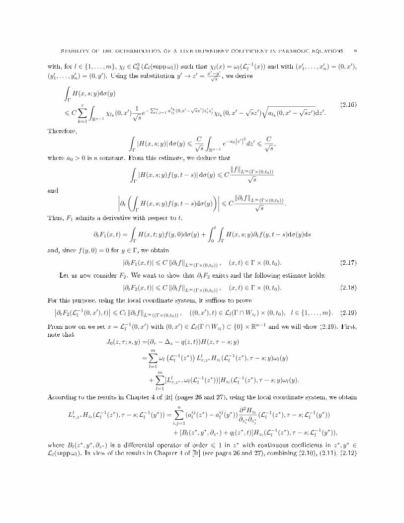
H(x, s; y)f(y, t− s)dσ(y)ds. (2.15)
Next, for x ∈ Γ, there exist l1, . . . , lr ⊂ 1, . . . ,m such that x ∈ suppωl for l ∈ l1, . . . , lr andx /∈ suppωl for l /∈ l1, . . . , lr. Moreover, since x ∈ Γ, we have zl1 , . . . , zlr ∈ Γ. Then, from the constructionof H(x, t; y), we obtain∫
Γ
H(x, s; y)dσ(y) =
∫Γ
r∑k=1
ωlk(x)Hzlk(x, s; y)ωlk(y)dσ(y)
= 2
r∑k=1
∫Rn−1
χlk(0, x′)1
(4πs)n2e−
∑ni,j=1
alkij
(0,y′)(x′i−y′i)(x′j−y′j)
4s χlk(0, y′)√alk(0, y′)dy′
STABILITY OF THE DETERMINATION OF A TIME-DEPENDENT COEFFICIENT IN PARABOLIC EQUATIONS 9
with, for l ∈ 1, . . . ,m, χl ∈ C30 (Ll(suppωl)) such that χl(x) = ωl(L−1
l (x)) and with (x′1, . . . , x′n) = (0, x′),
(y′1, . . . , y′n) = (0, y′). Using the substitution y′ → z′ = x′−y′√
s, we derive∫
Γ
H(x, s; y)dσ(y)
6 Cr∑
k=1
∫Rn−1
χlk(0, x′)1√se−
∑ni,j=1 a
lkij (0,x′−
√sz′)z′iz
′jχlk(0, x′ −
√sz′)
√alk(0, x′ −
√sz′)dz′.
(2.16)
Therefore, ∫Γ
|H(x, s; y)| dσ(y) 6C√s
∫Rn−1
e−a0|z′|2dz′ 6 C√
s,
where a0 > 0 is a constant. From this estimate, we deduce that∫Γ
|H(x, s; y)f(y, t− s)| dσ(y) 6 C‖f‖L∞(Γ×(0,t0))√
s
and ∣∣∣∣∂t(∫Γ
H(x, s; y)f(y, t− s)dσ(y)
)∣∣∣∣ 6 C ‖∂tf‖L∞(Γ×(0,t0))√s
.
Thus, F1 admits a derivative with respect to t,
∂tF1(x, t) =
∫Γ
H(x, t; y)f(y, 0)dσ(y) +
∫ t
0
∫Γ
H(x, s; y)∂tf(y, t− s)dσ(y)ds
and, since f(y, 0) = 0 for y ∈ Γ, we obtain
|∂tF1(x, t)| 6 C ‖∂tf‖L∞(Γ×(0,t0)) , (x, t) ∈ Γ× (0, t0). (2.17)
Let us now consider F2. We want to show that ∂tF2 exists and the following estimate holds:
|∂tF2(x, t)| 6 C ‖∂tf‖L∞(Γ×(0,t0)) , (x, t) ∈ Γ× (0, t0). (2.18)
For this purpose, using the local coordinate system, it suces to prove∣∣∂tF2(L−1l (0, x′), t)
∣∣ 6 Cl ‖∂tf‖L∞((Γ×(0,t0)) , ((0, x′), t) ∈ Ll(Γ ∩Wzl)× (0, t0), l ∈ 1, . . . ,m. (2.19)
From now on we set x = L−1l (0, x′) with (0, x′) ∈ Ll(Γ ∩Wzl) ⊂ 0 ×Rn−1 and we will show (2.19). First,
note thatJ0(z, τ ; s, y) =(∂τ −∆z − q(z, t))H(z, τ − s; y)
=
m∑l=1
ωl(L−1l (z∗)
)Llτ,z∗Hzl(L
−1l (z∗), τ − s; y)ωl(y)
+
m∑l=1
[Llτ,z∗ , ωl(L−1l (z∗))]Hzl(L
−1l (z∗), τ − s; y)ωl(y).
According to the results in Chapter 4 of [It] (pages 26 and 27), using the local coordinate system, we obtain
Llτ,z∗Hzl(L−1l (z∗), τ − s;L−1
l (y∗)) =
n∑i,j=1
(aijl (z∗)− aijl (y∗))∂2Hzl
∂z∗i ∂z∗j(L−1
l (z∗), τ − s;L−1l (y∗))
+ [Bl(z∗, y∗, ∂z∗) + ql(z
∗, t)]Hzl(L−1l (z∗), τ − s;L−1
l (y∗)),
where Bl(z∗, y∗, ∂z∗) is a dierential operator of order 6 1 in z∗ with continuous coecients in z∗, y∗ ∈
Ll(suppωl). In view of the results in Chapter 4 of [It] (see pages 26 and 27), combining (2.10), (2.11), (2.12)

10 MOURAD CHOULLI AND YAVAR KIAN
and (2.16), applying the substitution y′′ = z′−y′√τ−s , with z
∗ = (z∗1 , z′) and y∗ = (0, y′), we obtain∫
Γ
J0(L−1l (z∗), τ ; y, s)dσ(y) =
2∑j=0
Pj
(z∗1√τ − s
)e−
(z∗1 )2
τ−s
[∫Rn−1
Jj0 (z∗, τ ; y′′, s; τ − s)(τ − s) j2
dy′′
],
for 0 < s < τ < t0 and z∗ ∈ Ll(Ω ∩Wzk), where, for j = 0, 1, 2, Pj are polynomials and Jj0 are continuousfunctions, C1 with respect to τ, s ∈ (0, t0) and satisfy
maxi=0,1,2α1+α261
∫Rn−1
∣∣∣∂α1τ ∂α2
s Jj0 (z∗, τ ; y′′, s; v1)∣∣∣ dy′′ 6 Cl, 0 < s < τ < t0, z∗1 > 0, 0 < v1 < t0,
for some constant Cl > 0. We note that ∂v1Jj0 ((z′1, z
′′), τ ; y′′, s; v1) is not necessarily bounded. Indeed, weshow ∣∣∣∂v1Jj0 ((z′1, z
′′), τ ; y′′, s; v1)∣∣∣ 6 Cl√
v1, 0 < v1 < t0, j = 0, 1, 2.
This representation and the construction of K(z, τ ; y, s) in Chapter 5 of [It] (see pages 31 to 32 for theconstruction in Rn and page 53 for the construction in a bounded domain) lead∫
Γ
K(L−1l (z∗), τ ; y, s)dσ(y) =
2∑j=0
Qj
(z∗1√τ − s
)e−
(z∗1 )2
τ−s
[∫Rn−1
Kj (z∗, τ ; y′′, s; τ − s)(τ − s) j2
dy′′
], (2.20)
for 0 < s < τ < t0 and z∗ ∈ Ll(Ω ∩Wzk), where, for j = 0, 1, 2, Qj are polynomials and Kj are continuousfunctions, C1 with respect to τ, s ∈ (0, t0) and satisfy
maxi=0,1,2α1+α261
∫Rn−1
|∂α1τ ∂α2
s Kj (z∗, τ ; y′′, s; v1)| dy′′ 6 Cl, 0 < s < τ < t0, z∗1 > 0, 0 < v1 < t0,
where Cl > 0 is a constant. Furthermore, using representation (2.20), we have, for s < τ < t < t0,∫Ω
H(x, t− τ ; z)
∫Γ
K(τ, z; y, s)f(y, s)dσ(y)dz
=
2∑j=0
m∑l=1
∫Rn+ωl(x)Hzl(x, t− τ ;L−1
l (z∗))χl(z∗)Qj
(z∗1√τ − s
)e−
(z∗1 )2
τ−s
[∫Rn−1
Kj (z∗, τ ; y′′, s; τ − s)(τ − s) j2
dy′′
]dz∗
with Rn+ = (z∗1 , . . . , z∗n) ∈ Rn; z∗1 > 0. Then, applying the substitutions z′′ = x′−z′√t−τ and z′1 =
z∗1√τ−s , we
deduce, in view of the form of the functions Kj , the following∫Ω
H(x, t− τ ; z)
∫Γ
K(z, τ ; y, s)dσ(y)dz
=
1∑j=0
∫Rn+
H ′l(x′, t− τ ; (z′1, z
′′), τ − s)√t− τ
[∫Rn−1
K ′j ((z′1, z′′), τ ; y′′, s; τ − s)(τ − s) j2
dy′′
]dz′′dz′1, s < τ < t < t0,
(2.21)for some continuous functions K ′0, K
′1 and H ′l such that K ′0, K
′1 are C1, with respect to s and τ , and the
following estimates hold:∫Rn+|H ′l(x′, t− τ ; (z′1, z
′′), τ − s)| dz′′ 6 Cl, 0 < s < τ < t < t0, (2.22)
maxj=0,1
α1+α261
∫Rn−1
∣∣∂α1τ ∂α2
s K ′j ((z′1, z′′), τ ; y′′, s; v1)
∣∣ dy′′ 6 Cl, 0 < s < τ < t0, 0 < v1 < t0, (2.23)
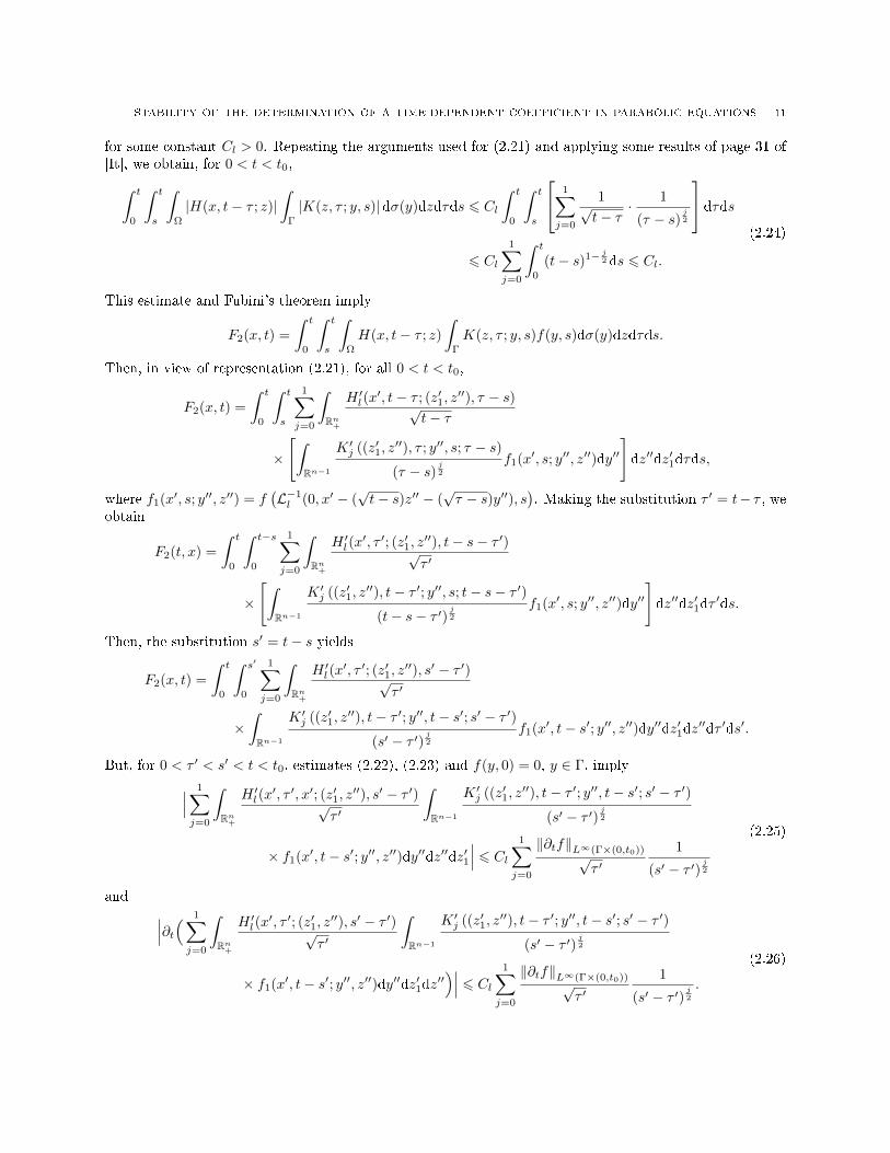
STABILITY OF THE DETERMINATION OF A TIME-DEPENDENT COEFFICIENT IN PARABOLIC EQUATIONS 11
for some constant Cl > 0. Repeating the arguments used for (2.21) and applying some results of page 31 of[It], we obtain, for 0 < t < t0,∫ t
0
∫ t
s
∫Ω
|H(x, t− τ ; z)|∫
Γ
|K(z, τ ; y, s)|dσ(y)dzdτds 6 Cl
∫ t
0
∫ t
s
1∑j=0
1√t− τ
· 1
(τ − s) j2
dτds6 Cl
1∑j=0
∫ t
0
(t− s)1− j2 ds 6 Cl.
(2.24)
This estimate and Fubini's theorem imply
F2(x, t) =
∫ t
0
∫ t
s
∫Ω
H(x, t− τ ; z)
∫Γ
K(z, τ ; y, s)f(y, s)dσ(y)dzdτds.
Then, in view of representation (2.21), for all 0 < t < t0,
F2(x, t) =
∫ t
0
∫ t
s
1∑j=0
∫Rn+
H ′l(x′, t− τ ; (z′1, z
′′), τ − s)√t− τ
×
[∫Rn−1
K ′j ((z′1, z′′), τ ; y′′, s; τ − s)(τ − s) j2
f1(x′, s; y′′, z′′)dy′′
]dz′′dz′1dτds,
where f1(x′, s; y′′, z′′) = f(L−1l (0, x′ − (
√t− s)z′′ − (
√τ − s)y′′), s
). Making the substitution τ ′ = t− τ , we
obtain
F2(t, x) =
∫ t
0
∫ t−s
0
1∑j=0
∫Rn+
H ′l(x′, τ ′; (z′1, z
′′), t− s− τ ′)√τ ′
×
[∫Rn−1
K ′j ((z′1, z′′), t− τ ′; y′′, s; t− s− τ ′)
(t− s− τ ′) j2f1(x′, s; y′′, z′′)dy′′
]dz′′dz′1dτ
′ds.
Then, the substitution s′ = t− s yields
F2(x, t) =
∫ t
0
∫ s′
0
1∑j=0
∫Rn+
H ′l(x′, τ ′; (z′1, z
′′), s′ − τ ′)√τ ′
×∫Rn−1
K ′j ((z′1, z′′), t− τ ′; y′′, t− s′; s′ − τ ′)
(s′ − τ ′) j2f1(x′, t− s′; y′′, z′′)dy′′dz′1dz′′dτ ′ds′.
But, for 0 < τ ′ < s′ < t < t0, estimates (2.22), (2.23) and f(y, 0) = 0, y ∈ Γ, imply∣∣∣ 1∑j=0
∫Rn+
H ′l(x′, τ ′, x′; (z′1, z
′′), s′ − τ ′)√τ ′
∫Rn−1
K ′j ((z′1, z′′), t− τ ′; y′′, t− s′; s′ − τ ′)
(s′ − τ ′) j2
× f1(x′, t− s′; y′′, z′′)dy′′dz′′dz′1∣∣∣ 6 Cl 1∑
j=0
‖∂tf‖L∞(Γ×(0,t0))√τ ′
1
(s′ − τ ′) j2
(2.25)
and ∣∣∣∂t( 1∑j=0
∫Rn+
H ′l(x′, τ ′; (z′1, z
′′), s′ − τ ′)√τ ′
∫Rn−1
K ′j ((z′1, z′′), t− τ ′; y′′, t− s′; s′ − τ ′)
(s′ − τ ′) j2
× f1(x′, t− s′; y′′, z′′)dy′′dz′1dz′′)∣∣∣ 6 Cl 1∑
j=0
‖∂tf‖L∞(Γ×(0,t0))√τ ′
1
(s′ − τ ′) j2.
(2.26)
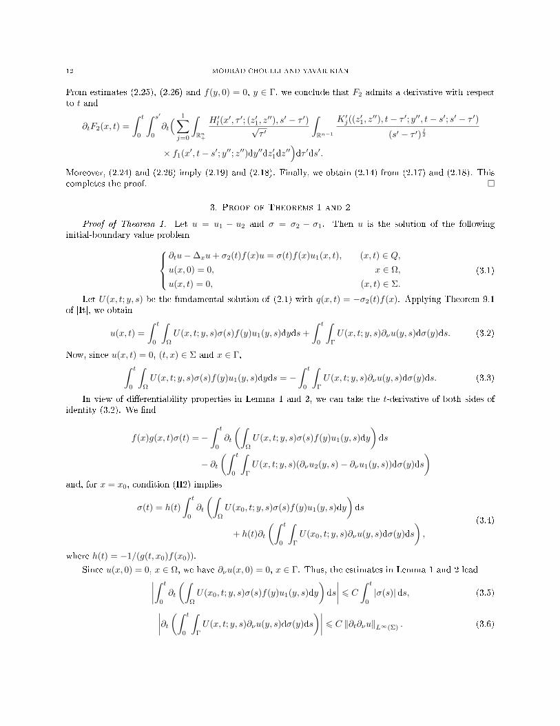
12 MOURAD CHOULLI AND YAVAR KIAN
From estimates (2.25), (2.26) and f(y, 0) = 0, y ∈ Γ, we conclude that F2 admits a derivative with respectto t and
∂tF2(x, t) =
∫ t
0
∫ s′
0
∂t
( 1∑j=0
∫Rn+
H ′l(x′, τ ′; (z′1, z
′′), s′ − τ ′)√τ ′
∫Rn−1
K ′j((z′1, z′′), t− τ ′; y′′, t− s′; s′ − τ ′)
(s′ − τ ′) j2
× f1(x′, t− s′; y′′; z′′)dy′′dz′1dz′′)dτ ′ds′.
Moreover, (2.24) and (2.26) imply (2.19) and (2.18). Finally, we obtain (2.14) from (2.17) and (2.18). Thiscompletes the proof.
3. Proof of Theorems 1 and 2
Proof of Theorem 1. Let u = u1 − u2 and σ = σ2 − σ1. Then u is the solution of the followinginitial-boundary value problem
∂tu−∆xu+ σ2(t)f(x)u = σ(t)f(x)u1(x, t), (x, t) ∈ Q,u(x, 0) = 0, x ∈ Ω,
u(x, t) = 0, (x, t) ∈ Σ.
(3.1)
Let U(x, t; y, s) be the fundamental solution of (2.1) with q(x, t) = −σ2(t)f(x). Applying Theorem 9.1of [It], we obtain
u(x, t) =
∫ t
0
∫Ω
U(x, t; y, s)σ(s)f(y)u1(y, s)dyds+
∫ t
0
∫Γ
U(x, t; y, s)∂νu(y, s)dσ(y)ds. (3.2)
Now, since u(x, t) = 0, (t, x) ∈ Σ and x ∈ Γ,∫ t
0
∫Ω
U(x, t; y, s)σ(s)f(y)u1(y, s)dyds = −∫ t
0
∫Γ
U(x, t; y, s)∂νu(y, s)dσ(y)ds. (3.3)
In view of dierentiability properties in Lemma 1 and 2, we can take the t-derivative of both sides ofidentity (3.2). We nd
f(x)g(x, t)σ(t) =−∫ t
0
∂t
(∫Ω
U(x, t; y, s)σ(s)f(y)u1(y, s)dy
)ds
− ∂t(∫ t
0
∫Γ
U(x, t; y, s)(∂νu2(y, s)− ∂νu1(y, s))dσ(y)ds
)and, for x = x0, condition (H2) implies
σ(t) = h(t)
∫ t
0
∂t
(∫Ω
U(x0, t; y, s)σ(s)f(y)u1(y, s)dy
)ds
+ h(t)∂t
(∫ t
0
∫Γ
U(x0, t; y, s)∂νu(y, s)dσ(y)ds
),
(3.4)
where h(t) = −1/(g(t, x0)f(x0)).
Since u(x, 0) = 0, x ∈ Ω, we have ∂νu(x, 0) = 0, x ∈ Γ. Thus, the estimates in Lemma 1 and 2 lead∣∣∣∣∫ t
0
∂t
(∫Ω
U(x0, t; y, s)σ(s)f(y)u1(y, s)dy
)ds
∣∣∣∣ 6 C ∫ t
0
|σ(s)| ds, (3.5)
∣∣∣∣∂t(∫ t
0
∫Γ
U(x, t; y, s)∂νu(y, s)dσ(y)ds
)∣∣∣∣ 6 C ‖∂t∂νu‖L∞(Σ) . (3.6)

STABILITY OF THE DETERMINATION OF A TIME-DEPENDENT COEFFICIENT IN PARABOLIC EQUATIONS 13
Therefore, representation (3.4) and estimates (1.5), (3.5), (3.6) imply
|σ(t)| 6∫ t
0
C |σ(s)| ds+ C ‖∂t∂νu‖L∞(Σ) .
Here and henceforth, C > 0 is a generic constant depending only on data. Hence, Gronwall's lemma yields
|σ(t)| 6 C ‖∂t∂νu‖L∞(Σ) eCt 6 CeCT ‖∂t∂νu‖L∞(Σ) , t ∈ (0, T ).
Then (1.3) follows and the proof is complete.
Proof of Theorem 2. Set u = u1 − u2 = u(σ1) − u(σ2). Then, according to (H4) and (H6), u is thesolution of the following initial-boundary value problem
∂tu−∆xu− q(x, t)u = F (t, x, σ1(t), u2(x, t))− F (t, x, σ2(t), u2(x, t)) , (x, t) ∈ Q,u(x, 0) = 0, x ∈ Ω,
u(t, x) = 0, (t, x) ∈ Σ,
(3.7)
with
q(x, t) =
∫ 1
0
∂uF [t, x, σ1(t), u2(x, t) + τ(u1(x, t)− u2(x, t))]dτ. (3.8)
Note that assumptions (H4) and (H6) imply that q ∈ C1(Q).
On the other hand, in view of (H4),
F (t, x, σ1(t), u2(x, t))− F (t, x, σ2(t), u2(x, t)) = (σ1(t)− σ2(t))G(x, t),
with
G(x, t) =
∫ 1
0
∂σF (t, x, σ2(t) + s(σ1(t)− σ2(t)), u2(x, t)) ds.
Using this representation, we deduce that u is the solution of∂tu−∆xu− q(x, t)u = (σ1(t)− σ2(t))G(x, t), (x, t) ∈ Q,u(x, 0) = 0, x ∈ Ω,
u(x, t) = 0, (t, x) ∈ Σ.
(3.9)
Let us remark that (H4) and (H6) imply that G ∈ C2,1(Q). Let U(t, x; s, y) be the fundamental solution of(2.1) with q(x, t) dened by (3.8). Then, according to Theorem 9.1 of [It], for σ(t) = σ1(t)− σ2(t), we havethe representation
u(x, t) =
∫ t
0
∫Ω
U(x, t; y, s)σ(s)G(y, s)dyds+
∫ t
0
∫Γ
U(x, t; y, s)∂νu(y, s)dσ(y)ds.
Since u(x, t) = 0, (t, x) ∈ Σ, we obtain∫ t
0
∫Ω
U(x0, t; y, s)σ(s)G(y, s)dyds = −∫ t
0
∫Γ
U(x0, t; y, s)∂νu(y, s)dσ(y)ds, (3.10)
with x0 dened in assumption (H5). Combining Lemma 1 and Lemma 2 with some arguments used in theproof of Theorem 1, we prove that f1 and f2 dened respectively by
f1(t) =
∫ t
0
∫Ω
U(x0, t; y, s)σ(s)G(y, s)dyds,
f2(t) =
∫ t
0
∫Γ
U(x0, t; y, s)∂νu(y, s)dσ(y)ds,
admit a derivative with respect to t and
f ′1(t) = σ(t)G(x0, t) +
∫ t
0
∂t
(∫Ω
U(x0, t; y, s)σ(s)G(y, s)dy
)ds,
14 MOURAD CHOULLI AND YAVAR KIAN
f ′2(t) =
∫ t
0
∂t
(∫Γ
U(x0, t; y, s)∂νu(y, s)dσ(y)
)ds,
∣∣∣∣∫ t
0
∂t
(∫Ω
U(x0, t; y, s)σ(s)G(y, s)dy
)ds
∣∣∣∣6 C
∫ t
0
|σ(s)| ‖G(·, s)‖C2x(Ω) ds 6 C∫ t
0
|σ(s)| ds (3.11)
and ∣∣∣∣∫ t
0
∂t
(∫Γ
U(x0, t; y, s)∂νu(y, s)dσ(y)
)ds
∣∣∣∣ 6 C ‖∂t∂νu‖L∞(Σ) . (3.12)
Here and in the sequel C > 0 is a generic constant that can depend only on data.
Taking the t-derivative of both sides of identity (3.10), we obtain
σ(t)G(x0, t) = −∫ t
0
∂t
(∫Ω
U(x0, t; y, s)σ(s)G(y, s)dy
)ds
−∫ t
0
∂t
(∫Γ
U(x0, t; y, s)∂νu(y, s)dσ(y)
)ds.
Let us observe that (H5) and max(‖σ1‖∞ , ‖σ2‖∞) 6M imply
|G(x0, t)| =∫ 1
0
|∂σF (t, x0, σ2(t) + s(σ1(t)− σ2(t)), g(x0, t)) |ds
> inft∈[0,T ],σ∈[−M,M ]
|∂σF (t, x0, σ, g(x0, t))| > 0. (3.13)
Then,
σ(t) = H(t)
∫ t
0
∂t
(∫Ω
U(x0, t; y, s)σ(s)G(y, s)dy
)ds
+H(t)
∫ t
0
∂t
(∫Γ
U(x0, t; y, s)∂νu(y, s)dσ(y)
)ds,
where H(t) = −1/G(x0, t). Hence, (3.11), (3.12) and (3.13) imply
|σ(t)| 6∫ t
0
C |σ(s)| ds+ C ‖∂t∂νu‖L∞(Σ) .
We complete the proof of Theorem 2 by applying Gronwall's lemma.
References
[CE86-1] J. R. Cannon and S. P. Esteva, An inverse problem for the heat equation, Inverse Problems 2 (1986), 395-403.[CE86-2] J. R. Cannon and S. P. Esteva, A note on an inverse problem related to the 3-D heat equation, Inverse problems
(Oberwolfach, 1986), 133-137, Internat. Schriftenreihe Numer. Math. 77, Birkhäuser, Basel, 1986.[CL88] J. R. Cannon and Y. Lin, Determination of a parameter p(t) in some quasi-linear parabolic dierential equations,
Inverse Problems 4 (1988), 35-45.[CL90] J. R. Cannon and Y. Lin, An Inverse Problem of Finding a Parameter in a Semi-linear Heat Equation, J. Math.
Anal. Appl. 145 (1990), 470-484.m[Ch91-1] M. Choulli, An abstract inverse problem, J. Appl. Math. Stoc. Ana. 4 (2) (1991) 117-128[Ch91-2] M. Choulli, An abstract inverse problem and application, J. Math. Anal. Appl. 160 (1) (1991), 190-202.[Ch09] M. Choulli, Une introduction aux problèmes inverses elliptiques et paraboliques, Mathématiques et Applications, 65,
Springer-Verlag, Berlin, 2009.[COY] M. Choulli, E. M. Ouhabaz and M. Yamamoto, Stable determination of a semilinear term in a parabolic equation,
Commun. Pure Appl. Anal. 5 (3) (2006), 447-462.[CY06] M. Choulli and M. Yamamoto, Some stability estimates in determining sources and coecients, J. Inv. Ill-Posed
Problems 14 (4) (2006), 355-373.

STABILITY OF THE DETERMINATION OF A TIME-DEPENDENT COEFFICIENT IN PARABOLIC EQUATIONS 15
[CY11] M. Choulli and M. Yamamoto, Global existence and stability for an inverse coecient problem for a semilinearparabolic equation, Arch. Math (Basel), 97 (6) (2011), 587-597.
[E07] G. Eskin, Inverse hyperbolic problems with time-dependent coecients, Commun. PDE, 32 (11) (2007), 1737-1758.[E08] G. Eskin, Inverse problems for the Schrödinger equations with time-dependent electromagnetic potentials and the
Aharonov-Bohm eect, J. Math. Phys. 49 (2) (2008), 1-18.[It] S. Itô, Diusion equations, Transaction of Mathematical Monographs 114, Providence, RI, 1991.[LSU] O. A. Ladyzhenskaja, V. A. Solonnikov and N. N. Ural'tzeva, Linear and quasilinear equations of parabolic
type, Nauka, Moscow, 1967 in Russian ; English translation : American Math. Soc., Providence, RI, 1968.[LS88] A. Lorenzi and E. Sinestrari, An inverse problem in the theory of materials with memory, J. Nonlinear Anal. TMA
12 (12) (1988),1217-1333.[LS87] A. Lorenzi and E. Sinestrari, Stability results for a partial integrodierential equation, Proc. of the Meeting, Volerra
Integrodierential Equations in Banach Spaces; Trento, Pitman, London, (1987).[PO85-1] A. I. Prilepko and D. G. Orlovskii, Determination of evolution parameter of an equation, and inverse problems
in mathematical physics I, Translations from Di. Uravn. 21 (1) (1985), 119-129.[PO85-2] A. I. Prilepko and D. G. Orlovskii, Determination of evolution parameter of an equation, and inverse problems
in mathematical physics II Translations from Di. Uranv. 21 (4) (1985), 694-701.[Sa] R. Salazar, Determination of time-dependent coecients for a hyperbolic inverse problem, arXiv:1009.4003v1.
Mourad Choulli, LMAM, UMR 7122, Université de Lorraine, Ile du Saulcy, 57045 Metz cedex 1, France
E-mail address: [email protected]
Yavar Kian, UMR-7332, Aix Marseille Université, Centre de Physique Théorique, Campus de Luminy, Case
907, 13288 Marseille cedex 9, France
E-mail address: [email protected]