ssc-342 global ice forces and ship response to … · ssc-342 global ice forces and ship response...
TRANSCRIPT

SSC-342
GLOBAL ICE FORCES AND
SHIP RESPONSE TO ICEANALYSIS OF ICE RAMMING FORCES
Thistiumcnthaskenapprovedforpublicrelemcaudr.alqitsClistlibutimisUrJjmjtd
wm STRUCTURE cOMMITTEE
1990

SHIP STRLJCVJRECOMMlll_FF
The SHIP STRUCTURE COMMllTEE is constituted 10 prosecute a research program to improve the hull structures of shipsand other marine structures by an extension of knowledge pertaining to design, materials, and methods of construction.
RADM J, D, Sipes, USCG, (Chairman)Chief, Office of Marine Safety, Security
and Environmental ProtectionU. S, Coast Guard
Mr. Alexander MalakhoffDirector, Structural Integrity
Subgroup (SEA 55Y)Naval Sea Systems Command
Dr. Donald LiuSenior Vice PresidentAmerican Bureau of Shipping
Mr. H. T. HalterAssociate Administrator for Ship-
building and Ship OperationsMaritime Administration
Mr. Thomas W. AllenEngineering Officer (N7)Military Sealift Command
CDR Michael K. Parmelee, USCG,Secretary, Ship Structure CommitteeU. S. Coast Guard
CON TRACTING OFFICER TECHNICAL REPRESENTATIVES
Mr. William J. SiekierkaSEA55Y3Naval Sea Systems Command
Mr. Greg D. WoodsSEA55Y3Naval Sea Systems Command
SHIP STRUCTURE SUBCOMMllTEE
The SHIP STRUCTURE SUBCOMMllTEE acts for the Ship Structure Committee on technical matters by providing technicalcoordination for determinant ing the goals and objectives of the program and by evaluating and interpreting the resu Its interms of structural design, construction, and operation.
AMFRICAN RUREAU O F SHIPPING
Mr. Stephen G, Arntson (Chairman)Mr. John F. ConIonMr. William Harrzal@kMr. Philip G, Rynn
MILITARY SEALl~ COMMAND
Mr. Albert J. AltermeyerMr, Michael W. ToumaMr. Jeffery E. Beach
M Al SPA Wv STEMS COMMAN~
Mr. Robert A, SielskiMr. Charles L. NullMr. W. Thomas PackardMr. Allen H, Engle
U. S. COAST GUARD
CAPT T. E. ThompsonCAPT Donald S. JensenCDR Mark E. Nell
MARITIME ADMINISTRATION
Mr, Frederick SeiboldMr, Norman O. HammerMr. Chao H, LinDr. Walter M. Maclean
SHIP STRUCTURE SUBCOMMllTEE LIAISON MEMBE!=IS
~
LT Bruce Mustain
I I S, MERCHANT MARIN.E ACADFMY
Dr. C. B. Kim
U.S. NAVAL ACADEMY
Dr. Ramswar BhattachWa
STATE UNIVERSIW OF NEW YORKMARITIMF C(3I I FGF
Dr. W, PI. Porter
WELDING RESEARCH COUNCIL
Dr, Martin Prager
~-MARINE BOARD
Mr. Alexander B. Stavovy
NATIONAL ACADEMY OF SCIENCES -COMMlll_EE ON MARINE STRUCTURES
Mr. Stanley G. Stiansen
SOCF o NAVA L ARCHITECTS ANITMARl~E E~GINEERS -HYDRODYNAMICS COMMllTEE
Dr. William Sandberg
~MFRICAN IRO N AND STEFI INSTITU TE
Mr. Alexander D. Wilson

Member Agencies:
UnitedStates Coast GuardNava/ Sea Systems Command
MaritimeAdministrationAmerican Bureau of Sh@ping
MilitarySealiftCommand
ShipStructure
CommitteeAn Interagency Advisoty Committee
Dedicated to the Improvement of Marine Stnxtures
December 3, 1990
Address Correspondence to:
Secretary, Ship Structure CommtieeU.S. Coast Guard (G-MTH)2100 Second Street S.W.Washington, D.C. 20593-0001PH: (202) 267-0003FAX: (202) 267-0025
SSC-342SR-1313
GLOBAL ICE FORCES AND SHIP RESPONSE TO ICEANALYSIS OF ICE RAMMING FORCES
This report is the fifth in a series of six that address iceloads, ice forces, and ship response to ice. The data for thesereports were obtained during deployments of the U. S. Coast GuardIcebreaker POLAR SEA. This report supplements SSC-341, GlobalIce Forces and Ship ResDonse to Ice and contains a discussion ofthe finite element model that was developed to predict iceramming forces. The other ice reports are published as SSC-329,SSC-339, SSC-340, SSC-341 and SSC-343.
J~. SIPESRear Admiral, U.S. Coast Guard
Chairman, Ship Structure Committee


Tcclmica[ Report Documentutian Page
1. Report NQ. 2. Government A=cesxien No. 3. Rocipienr’s Catalog No.
SSC-342I I
4. Titlm and Subtitle I 5. Reoart Date
Global b Foroesand Ship Response to Ice - Analysisof Ice Ramming Foroes
7. Authods)[ S. Porferming Organization Report No.
I ABS Tech. RPt. RD-8701 IYung-Kuang Chen, Atfred L. Tunik, Albert P-Y Chen
9. pdmrninq Otgmi zotion Nom. d Addrmss
AMERICAN BUREAU OF SHIPPING
- OED-8752210. wok Unit No. (TRAIS)
45 Eisenhower DriveParamus, NJ 07853
13. Typo of Report and Psriad Caverod
1Z Sponsoring Aq.ncy Namm -d Addt*** Transport Development Ctr~Maritime Admi nitration 200 Dorchester Blvd. ,West Final ReportU.S.Dept. of Trans Suite 601, West Tower400 Seventh Street, SW Montreal, Quebec 14.Sponxaring Agency Cad,
Nashin ton D.C. 20593 H~ MAR-760 ~15. &#ppklMtmy Natos This was an international joint project between the Ship Structure
Committee (USA) and the Transport Development Centre (Canada). The U.S. MaritimeAdministration served as the sponsoring agency for the interagency Ship StructureCommittee.
‘h”‘b’tr”’tlluringSeptember and October of 1985 the Polar Sea conducted ice-impacttests on heavily ridged ice features in the Alaskan portion of the Beaufort Sea.Bending strain gage measurements were used to estimate the longitudinal bendingmoment distribution of the POLAR SEA during impacts with ice pressube ridges.Compressive strains along the stem and ship acceleration and velocity meas~rementwere also recorded. This paper describes the methodology for determining theglobal ice impact force from the measurements and presents the results of thesetests. A comparison of the results with other available data is also presented.Hull strain, and impact force time histories are presented along with thelongitudinal bending and shear distributions during ice impact events. Theresults indicate that the methodology used in estimating the impact forceprovided and excellent understanding of”ship-ice interaction.
This supplement to the main report(GlobalIceForcesand shipResponse to Ice, SSC-341 ) mntains adiscussion of afinite element model that was developedto predict ioe ramming forces and includes acomparisonof the model’sresultswith seleoted rammingevents.
)7. K*Y Words
Desian Criteria18. Distribution $tet.m~t
Document is available to the U.S. PublicIce [oads through the National TechnicalIcebreakers Information Service, Springfield, VAShipboard Loads Measurement 22161
I19. s~rity Clan*if. (Of this *art) ~. Soawity Classif. (of this peg-) 21.No.ofPag*s 22.Prico
Unclassified Unclassified
FOrmDOTF 1700.7 (8-72! Reproduction of complwtod page autherizod
I

METRIC CONVERSION FACTORS#
—23
— 22
—21
—20
—10
— la
—*7
— la
—18
—14
—13
—*2
—11
—lo
—0
—0
—7
—6
—s
—4
Appmximw Caiwmkm horn Mstrk Mswros
When Yw Kruw ktltwv h To Fid symbol
LEMGT14
mUtlfrwta9 OmWvbwmtus 0.4llwtao 3.3 tam
1.1 ~ordtMlalntut O.a mltn
Approabm- ~kltl$~O Matrk Mosum8
=—-
—-=
—.
==
-=2-
=—-
—2
—t

TABLE OF CONTENTS
1. INTRODUCTION
2. RAMMING FORCE ANALYSIS
2.1 ANALYTICW MODEL
2.2 GENEUL EVALUATION OFTHE TEST RECORDS
2.2.1 ForceRecords
2.2.2VelocityRecords
2.3 ANALYSIS OF THE GLOBAL FORCES
2.3.1
2.3.2
2.3.3
2.3.4
2.3.5
2.3.6
2.3.7
Analysisof theForceHistoryRecords
ShipMass
Bow Shape Factor
IceRidge Shape
Dynamic CrushingStrengthof Ice
ImpactVelocities
lmPactForces
3. HULL STRUCTURAL RESPONSE
3.1 METHOD OF ANALYSIS
3.2 MATHEMATICfi MODELLING
1. Three-dimensionalFiniteElement Model2. Buoyancy Springs3. Boundary Conditions4. Loading Conditions5. Hydrodynamic Added6. Damping
3.3 FREE VIBR4TIONANWYSIS
Mass
3.4 DYNAMIC STRUCTURAL ANALYSIS
1. Problem Formulation2. IceimpactLoads
3.5 DISCUSSIONOF RESULTS
4. CONCLUSION
5. REFERENCES
APPENDIX A FiniteElementModel
PageNo
1
2
2
3
3
3
10
10
17
17
20
22
22
26
30
30
31
313335353536
39
46
4647
55
103
106


.l.MERICA\ 13L2%EAL OF SHIPPI>”G
1. INTRODUCTION
The strain gauge measurement records acquired during the USCG POLAR SEA win-ter deployment represent a unique data base for predicting ice induced forcesdue to ramming icebreaking. The overall objective of such tests is aimed at de-velopment of an analytical model capable of describing the ship/ice impact
interaction. The model can be used as an effective tool in developing rationalstrength standards, in designing icebreakers and icebreaking cargo ships, in
evaluating ultimate capabilities of the ships in various ice conditions andother applications.
Two principal questions arise when analyzing the data and developing a model.First, what is the nature of relationships between the ice-induced load parame-ters (pressure, total force, dutation and time history, etc.) and the initial
impact characteristics (the masses, rigidities, mechanical properties of the
ship and the ice, and their impact velocities and locations). Secondly, what is
the relationship between the actual ice load parameters and the measured re–sponse of the ship structure, or in other words, how to interpret the recorded
data. This report is addressed to answering both questions.
In Section II the analytical model of ship/ice interaction is briefly de-scribd. The recorded data of the ramming forces, their durations and time his-tories, ramming velocity records, and the locations of the ramming forces are
analyzd and compared with those predicted by the analytical model for the ac-
tual testing conditions. The work releated to this section was performed by theOcean Engineering Division of the American Bureau of Shipping.
In Section 111 the dynamic response of the hull structure subject to variousimpact loads is analysed. The purpose of this analysis is to justify the appli-cability and determine the accuracy of the beam idealization used in interpret-ing the ice impact load measurements, as well as to study in detail the dynamicreponse of the complex hull structure to time varying impact loads due toramming icebreaking. The work of this section was carried out by ABS/Researchand Development Division.
The dynamic structural analysis was performd using a three–dimensional fi-nite element model representing the entire vessel including the deckhouse andother superstructures. At the forward end of the vessel where the ic~ impactloads occurred, a fine mesh model was used to connect through a transition seg-ment to a coarser mesh representation of the remainder of the vessel. This isto ensure that the structural response in the areas of interest could be deter-mined accurately.
A free vibration analysis was first carried out to determine the natural fre-quencies and mode shapes representing the coupled hull girder and deckhouse vi-bration. Then, a forced vibration was performed to obtain the transientresponse of the vessel to time varying impact loads. The ice impact loacs usedin the analysis were obtained from the measur~ data corresponding to Ram 14 andRam 39. Case studies were also included for ice impact loads with predefine
shapes of time functions, including the AM analytical mdel described in Sec-tion 11.
-1-

2. RAMMING FORCE ANALYSTS
2.1 ti~ymctiMODEL
A-
13-
CB -
D-
d-
Fn -
Fv -
F(t) -
R-
s-
T-
t-
P-
4-
Nomenclature
parameter characterizing dynamic crushing strength ofice, MPa(s/m3)1/4;
ship breadth, m;
block coefficient;
displacement measured in force units, MN;
ship draft
global impact force normal to the stem, MN;
vertical component of Fn, MN;
dimensionless force history factor which is force Fn atinstantaneous time 11t,1 normalized with respect to itsmaximum;
parameter characterizing ridge size, m;
shape factor
peak force duration, sec
dimensionless instantaneousto T;
frame flare angle between
time normalized with respect
the vertical and the frametangent line measured at the stem line in the verticalplane perpendicular to the center plane, (see Fig. 6),deg. ;
stem inclination angle to the horizon, (see Fig. 6),deg. ;
In accordance with the overall objective of the POW SEA deployment,the ice loads recorded during ramming ice-breaking should be used as adatabase for development of an analytical model. The model is to becapable of predicting impact ice loads on ships of various displacementsand shapes navigating in various ice conditions.
The analytical model, of solid/ice impact developed by Kheisin andKurdyumov in 1970’s [3; 4] appears to be most suitable for this purpose.In a generalized form [7] the model describes the ice impact loads on
-2-

ships as functions of ship and ice masses, their dimensional andinertial characteristics, contact zone shapes, the mechanical propertiesof ice, and the relative impact velocity.
It should be emphasized that the model describes the impact penetrationof a solid into ice. Static or quasi-static interactions are beyond thescope of this model. Ship/ice interaction during ramming has usuallytwo distinguishable phases: the initial phase of impact penetration intoice accompanied by ice crushing, and the following beaching phase.Higher forces are usually (but not necessarily) generated during theimpact phase. In this report only the impact forces clearlydistinguishable in the records are analyzed using the analytical model.
The model has been used to analyze impact ice loads for thefollowing applications:
- field tests of a steel ball dropped on flat ice surface[3, 4 and others];
- laboratory tests of a steel pendulum impacting ice samples[2, 7];
- ramming ice-breaking [8];
- iceberg / structure impacts [1, 6].
For icebreakers ramming mass ive ice features the ice loadparameters are expressed in [8] as follows:
Fn = KFDdVvAaSF(t)
T ==~DV/Fn
(1)
(2)
where coefficients (KF, KT) , exponents (d, v, a), force time historyfactor F(t) and shape factor (S) vary depending on particular slopes ofthe ship bow and the ice feature. For ramming ice-breaking the range ofvariations of the exponents and force history factor is given in Table 1and Figure 1 whose data represent some idealized shapes of ships andice.
TABLE 1
Exponent Wedge-shaped bow Spoon-shaped bowRectangular Rounded Rectangular Roundedice edge ice edge ice edge ice edge
d 5/7 7/11 2/3 5/9v 3/2 15/11 17/12 11/9a 2/7 4/11 1/3 4/9
-3-

0.728
0.67
III0.75
a 1
.
1
0./
0.(
0.1
0.:
0 /(, ,// ~.2
*1
//
/7o
0.2 0.4 0.6 0.8 1.0
dimensionless time, v=t/T
Fig. 1. Theoretical force time history curves
used in the analysis
. . predicted for drop ball test.—-.—_ predicted for a side impact
-4-

Those idealizations represent some extremities limiting the actualshapes. Thereforej the numerical values of the exponents should beselected within the range of the extremities. The values selected forpractical applications should be regarded as approximations.
The coefficients (KF and ~) also incorporate various idealizations and.$implifications used in deriving equations (1) - (2) (e.g. added watermass effects, ice edge spalling effects, pressure distribution over thecrushed ice layer’s thickness, etc; for details - see [4; 7]). Inpractical applications, their numerical values should be adjusted inaccordance with test data.
The POLAR SEA has a wedge-shaped bow, though not the perfect wedge. Herbow flare angles at the stem are very high (exceeding 60°) while thestem inclination angle is small (less than 20° at the design waterlinearea) and variable. Such a dull wedge can be treated as an intermediateshape between the perfect wedge and a spoon-shaped bow, though muchcloser to the wedge.
The shapes of ice ridges vary greatly and individual ridges can differsignificantly from each other and from any idealization. Such varietyof shapes was also characteristic for the ridges being rammed during thedeployment (see survey data in ref. 18 of the Report). Moreover, theyare often composed of separate ice blocks connected more or lessloosely. The presence of multi-year. ice inclusions was observedvisually. Coring and thermal drilling also showed the presence of largecavities .
For such testing conditions the values of exponents given in thirdcolumn of Table 1 or slightly lower can be most suitable. In thisanalysis the equations (1) and (2) are used in the following form:
Fn = 0.22D7/11 V15\11 A4/11 S 1? (t) (3)
T = 0.06 DV\Fn (4)
where: S = R3/11 Sb (5)
R - parameter characterizing ridge height.
‘b - (0.5 tan~ sin2p)4/11 sinq[(q+tan2q) cos2q]7/11 (6)
q = [1 + 2 Cw2B/d ‘1 + 3.57”[1+ / -1
3 CB(l+C )1 c (3-2CB);3-C ) ](6a)
w B w w
CB - block coefficientCW - waterplane coefficientB/d - breadth-to-draft ratio
The relationship between the vertical and normal components of theglobal force is:
-5-

Fv = Fn COS(O (7)
2.2 GENEW EVALUATIONOFTHETESTRECORDS
2.2.1 Force Records
Of the thirty eight ram records listed in Table 2 and 6 of the ARCTEC’SReport, only the records of the rams for which higher forces have beenrecorded are requested for the analysis. The submitted records containalmost all peak forces exceeding 14 MN. The 25-second records of theglobal force and velocity histories are reproduced in Figures 2a through2n.
It should be kept in mind that global ramming force records are not whathad been directly measured during the trial. The sensors have
registered strains in ship structures, and the measured strains areconverted to stresses based on the linear stress-strain relationship.The next steps of expressing the bending moments and shear forces viathe stresses are based on beam theory with some idealizations andapproximations of the stress distribution in the hull girder acted uponby a bow force.
The beam idealization used in the Arctec’s program can result in someinaccuracy when interpreting the strain gauge readings into verticalramming forces. However, such inaccuracy, if found, can be of a
systematic type and does not affect the capability of the analyticalmodel to fit and explain the experimental data. Therefore, the forcerecords presented in Figure 2 are presumed to be true sensor readings.
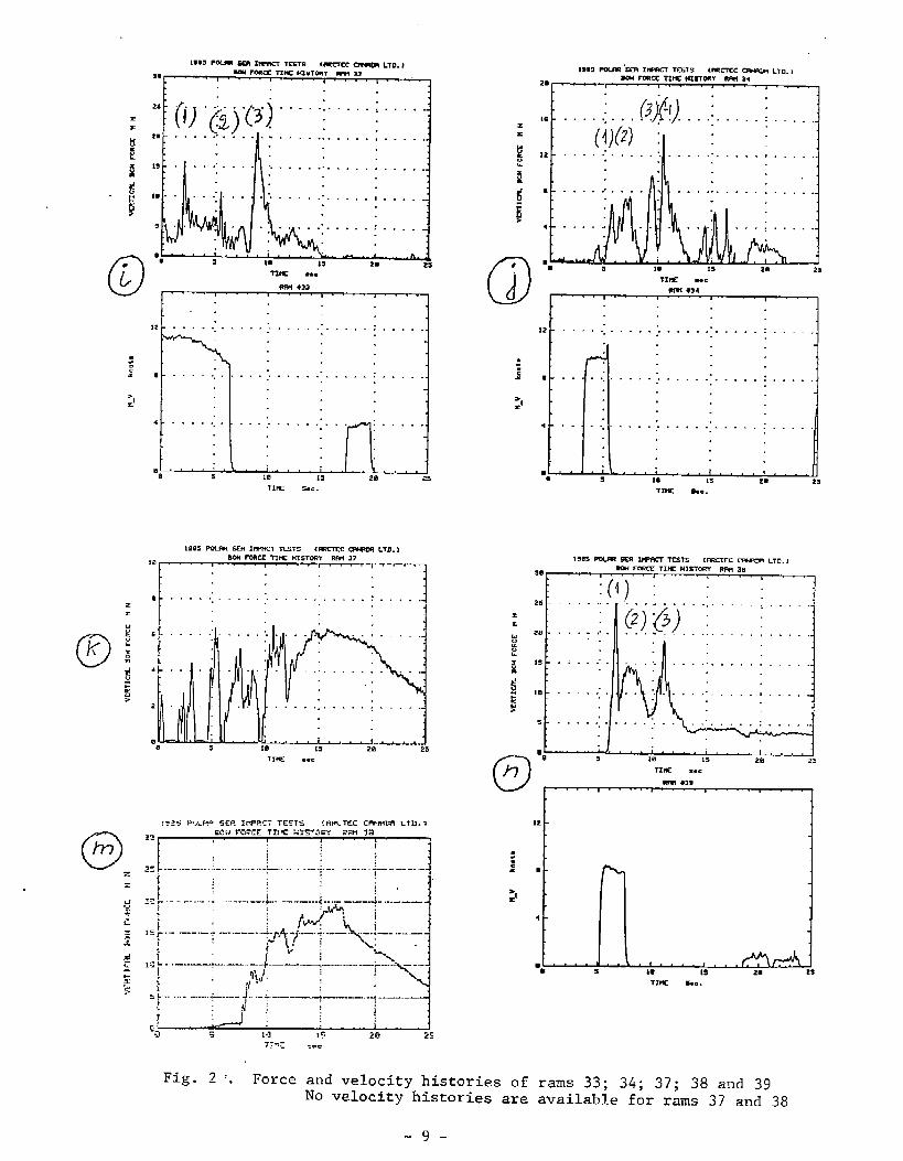
All of the force records in Figure 2 distinctly show a peak at thebeginning of the ram. For a number of events there are several peaksduring the ram. Durations of each peak force do not exceed 1.0 - 1.5seconds. For some events there is only a single peak followed by asignificantly lower beaching forces <rams 2, 14, 15, 25). For rams 37and 38 beaching forces are of the same or higher values as the initialimpact peak forces. The beaching force duration range typically from 5to 10 seconds but can be longer as recorded for rams 37 and 38. Thepresence of several peaks (rams 3, 9, 17, 26, 33, 34, 37) implies thatthe rammed ice ridges were composed of several ice hummocks or blocksrelatively loosely connected with each other - the fact which wasactually recorded in the ridge survey report (see ref. 18 of theReport). However, “from the field suney data it is impossible tospecify the separate ridge components. Ram 38 is the only ram for whichthe beaching force exceeds the initial impact force and, moreover, thelatter is not easy to distinguish. This ram record is not included forfurther analysis of the impact forces.
2.2.2 Velocitv records
Ship speed histories recorded from doppler log readings for the rams inquestion are shown in Figure 2 right under corresponding force records,except rams 37 and 38 for which the speed histories are not available.
-6-

oa
Jg= Pmm Sm lFwrr TCST5 (-~c -C+ LTn. >2E mm ~~= Tlnz H!sTwrf Rml z
I
16 . . . . . .. . . . . . .. .,=. . . . . . . . . . . ,.
12 - . . . . .. . . . . . .. . . . . . . . . . ,,, ,, ,
n- . . . . .. . . . . . . . . . . . . . . . . . .. .
4 . . . . .. . ..+. .,, , -. .:, ,,, ,
@e 5
TIIE .-=
1“’””’”’””’””’’”””~ 42
‘---1
.:1.
0c
‘aLB ,~,-, -!/2n 25
TIHE S=.
Tlw ,.=--
1:2s ............ ,,
zx
2E . . 4........ ,,, ,L!~
SIs.’...: -. .-’....m
i: ,e
. . . . .. . . . . ,-, ,.kY
. . .. . . . . . . . ... .1
...........,,.\I .. . . . . ,. .,, .,
.. . . . . .:, ,, . .
s . . . . . .. ,. ... ., .,,,
(2)>,;m0 5 10 15
T1tE .,.
m +14
Fig. 2 . Force and velocity histories of rams 2; 3; 9 and 14
-7-

(3e
16 . . . . . .. . . ...”.................,_
..............
e - ... ,,. ,+, ,. ,,
4
15
71- . . .
k-a.! ● 15
1~
. . . . .1...........................,..,.,,..-,,.,,.*.......,19BS POLFiR SW! lIIPHCT TESTS (Wc’rrc mwm LTD. ,
mm W(?CE TIM HIsTaw RM >=
L I 1
u
WI................,,.,..,,:,,..%-----.,....’-. . . . . . . . . . . . . . . .
:
;14 . . . -.’...... . . . .. . . . . . . . . . . .
.’
2 . . . . . . . . .. . . . . . . . . . . ,: . . . ,.
● .—.. ------~m s Im 1s 20 2s
TIM h..
@
I
l“.......,:,.,,..............Kl:;..... .....
15 2)3
~: : , ,
TIHE %..
1-*$ Pam s 1- ms t— — LTD. )
ammu+ fm TInz I.llrmmy m *g
1
25 . . . . . . . . . . . . . . . . . . . . . . . . . . . . . .
IL] TIK ..o
TIME *C.
Fig. 2 . Force and velocity histories of rams 15; 17; 25 and 26
-8-
la
12
●
4
●m5 10 is zm 2s
‘J’!y,w-llL--:----/●
● s
w.
19 15 29 25nnc . . .
12 . . . + . . . . . ...”... . . . . . . . . . . . . . . . .
# - . . . . . . . ,. ..-. . . . . . . . . . . .: .,. . .
* - . . . ..- . . . . . . ., +.. . . . . . . . . . .
“eL
sL
10 15 213 Zs
I12...+.:.....”..................IF
1 - . . . . .. . . . . .. . . . . . . . . . . . . . . . . .
I4 - . . . . .. . . . . . .. . . . . . . . . . . . . . . . .,
● . LJ, ,,4, ,,; ., J,;,,.,-● s 18 13 Zm 2s
19US - * IWwn TEs’rs [METCC -m LTD. )
10W FmCE TIIS HISTMY RFW 97
,-—--1. -—
1
Ims Pam m 1- TESTS [-CC ~ LTD. ,- ~MCE TIE HISTCUY PM 33
am
“:(,”)””; : :2$ -- . . - ...-..+... . .:.....:...,..
zx : (2)@J) : ,
Za -. ..-,.. . . . . . . . . . . . . . . . ,, . . . ..5 . ..2 I
is -. ~-.:. . . . .. . . . . . . . . . . . . . . . ,-5
;
Es- . . . . .. . . . ..”.
)
0, ..........❑
H “ ‘ ‘:’:●,:’” 29 25
0
t
.: ... .z.””””’.”” ““”.””””’”.””” “. jI
T]* . . .
}
Fig. 2 . Force and velocity histories of rams 33; 34; 37; 38 and 39No velocity histories are available for rams 37 and 38
-9-

Doppler logs usually give reliable and sufficiently accurate informationon ship speed in broken ice. However, the speed records shown in Fig. 2contain certain contradictions. For a number of rams the speed recordsare interrupted (rams 3, 9, 14, 33, 34, 39). It is supposed that the
drops occurred whenever the doppler radar failed to receive an echo.Probably the same cause can explain such speed records as those of rams15, 17, 25, 26. With this explanation the speed records with relativelyshort-time drops could be somehow bridged. However, the accuracy of thebridged records would be questionable. At best, it can give only anestimate of the velocity changes after initial ship/ice contact. Nosuch estimates are possible for rams 3, 15 ,17, 25, 26. For ram 34 thegap between the drops was almos~ 20 seconds during which time the effectof the propeller thrust on the speed can be noticeable. Therefore, onlythe initial speed data recorded prior to ship/ice ridge contact can beassumed reliable. The estimates made by bridging the velocity gapsshould be treated cautiously and compared with the estimates based onother sources.
In addition, the radar measured’ only the horizontal speeds. Vertical
and angular speed components (heaving and pitching) have no-t beenmeasured; so were the accelerations. Therefore, the speed records donot provide sufficient data to describe the kinematics of the rams,which, in turn, makes it difficult to analyze the interaction forces.This is especially so at the post-impact beaching phase when thevertical components of bow speed are essential.
2.3 ANALYSIS OF THE GLOBAL FORCES
2,3,1 Analysis of the Force Historv Records
Each distinct peak on the force history records isseparate impact. All of the impacts are analyzedequations (3) - (4). Fig. 3 shows a comparison of
considered to be ain accordance withdimensionless force
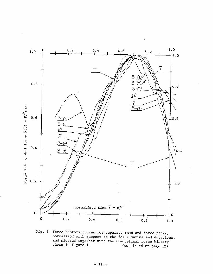
histories predicted theo~etically (Fig. 1-)and recorded (Fig. 2). Thepeak force records stretched in the time scale are normalized withrespect to their maxima (F = F/F~ax) and peak durations (t = t/T). Theduration “T” of a peak force record is determined by fitting togetherthe theoretical (Fig+ 1) and recorded pulses. Fig. 4 shows individualcomparisons of the dimensional peak forces with the force history curveof Fig. 1 dimensionalized with respect to the recorded maximum force andthe duration (i,e. the maximum predicted forces are assued equal to the.recb;ded peaks).
As seen from Fig. 3 and 4 the theoretical model fairly well describesthe impact process in time. For rams 2, 3-(l), 3-(4), 14, 15, 17-(2),34-(3), 34-(4), and 39, the theoretical curve fits the records almostperfectly.
The force history records differ from the theoretical curve mainly attheir lower ascending and descending branches: The beginning of impactinteractions is often influenced by the ice features situated in frontof the ridge, whereas the latest impact stage is influenced by the post-
-1o-
0 0.2I
0.4 0.6i I
0.8I —.___
Ir 1 I
------“ 4
/-”*\,#
\-
i“*./ /-+ ;fi/;
I
\l
‘--=-.._T_/
“1.0
normalized time t = t/T
1tI I 1 i“ I 1 I tI I
o 0.2 0.4 0.6 0.s 1.0
1.0
0.8
‘..,
k
“\
0.6
+;\
\o.4
\
0.2
)
Fig. 3 Force history curves for separate rams and force peaks,normalized with respect to the force maxima and durations,and plotted together with the theoretical force historyshown in Figure 1. (continued on page 12)
-11-

0.4‘0 ‘t+-m~–. , 0.6I 0.8
0.8
0.6
0.4
0.2
0
19 -(d)
-------17”(3)
/“..-....
.,”
-J.-p /‘/ i,d.2;;,
0
normalized time ~ = t/T
\
,0‘1.0
0.8
).6.,.“
/’
jl.4-+
I\\i,“9.2
\,
\
I I I I In.7 1 I In) 1 * o
.
U.4 0.6 0.8 1’.0Fig. 3 (continuation) ~~ ..
-12-

1.UI
I
Il“- ---~
0.2 0.4in 0.6 0.8 1.0I I4 1 I/“~+a +----i. 1.0
0.8
0.6
0.4
—,. , 39-(t)__--=,\\
T
—
1-
normal’izedtime ~ = t/To I I I I I ! I
0.I
0.2 0.4 “I
0.6 0.8 1.0
-----
‘k\‘ 0.6-\
\
‘L
0.4
0.2
o’
‘ig. 3 (continuation>
-13-

---1,
[r” 11 ,“~– ..-”’!.:! ‘ J’-’‘:Tz~-’~~”115. . . . . . .. . . . . . . ... ...”-..’ ~’.-.i
—-- ,. ‘ I ,,, ., ““- $-LSM’RJ=!..,-............,.,.,,,,,,.,119 . . . . . . . . . . . . . . . . . . . . ...-!
. . . . . . . . . . . . .““-”~:m:..................L‘--~:[~~-~--~=.;6k
am . . . . .. . . . . . :, . . . . . . . . . . . . .
*3.....:.....:. , . . . .. . . . . . . . . . ..,,,,
‘*1a
TIME(SCC).
j,. . ... . ,. ._, ,;.=
4
L
:. ...’ ;0
;&
. . . . . . . ..: i!jig,j]>7
.-.l,;.,.+.,....j0..sI
,,. ,
.. (\......:...:.......m.
. . . . . .
1.i’<’f’r”-’b
L -., z.,
.1.1......1[
..
i
1
Uz, ; !Im . . . . .. . . . . . .
~,, j ‘“.-..’’”:””--”:”””’” : 53s;. .,..
cr.,
1- . . . . . .. . . . . . . . . . . . . . . . . . . . . . . .0-44
. . . . . . . . .. . . . . . . . . . . .: . . . . .
●i . . . . . ....”... . . . . . .. . . . . . . ... ,.... . . . . . . . . . . . . . . . . ,
U* ,, . ,c~.,17.3 ,7., ,m., ,m.,rnsa
‘:1 21., ** Zz., ~, *>,, I,Itc rstc, ,., ,.+, ,,:;
T- IsCcl TIPC #xc>
Fig. -4 Recorded force histories as compared with the theoretical curve ofFig. 1 dimensionalized with respect’ to the recorded peak force.The load location records of the recorded peak forces are placedbelow the”corresponding force records at the same time scale.
(continued on page 15)
-14-

,- — mm ,— n,,, tmc’mc — L*..,
I*xu r- TM umTm m v.
“:-70.. — m ,— m., ,— — ~,o.,
I&r.w rmcr ‘II* “,m m ,,
f
Ii ~.-.
.* -,.
. -.. .
l-+=% ““,,..., —.1
I]s t . . . . . . . . . . . . . . . . . . . . .
1 J
“t :11:5 ----------- . . . . . . . . . . . .. . . . ., w,,
..........................:......WW
0“,7
Cr>?
C,=m
W* ● 1100 . . . . . . . . . . . . . . . . . . . . . .
. . . . . .. . . . . .. -----, ------ .-, ,.
,1.. ,i. , ,.. < ,*, C ,?
i9“5 . . . . . . . .. . . . . . . . . . . . . . . .m,,
rm sI 4-----: ..L–=1.,aL3- 10.7
TX-C lSCC)SW 1 113 13.1 13. B
TIHE (SEC>
U..........................:,.~...:.......Y., *.
. . . .. . ,, .,,. 1-1 J..,,.-:,..-.........,,............,,
,.
K12 . . ...’... .“. .,
s~:* .....,....:.,.#x~. . ................
●,, ,.* ,,.,3!i!!!l?....,,.,,....,.......,,.’, .,. .
-,? ,.s Is
{
LQ_-J1>.2 O*. C!.!---==.-
,-3 - m ,-, ,C,,. ,=.C _m ~,u.,Lwn,,c.1 w Lmo m +r ,,-(5)
. . . . . . . . . . . . .. , ., .,.,,..,
. . . . . . . . . . . . . . . . . . . . . . . ~,,
~
i. . . . . . . . . . . . . ..”
g
. . . . .. . . . . . . . ,’
,1.. ,,., ,*. * ,*. CTmc l=C>
L-71w4 w Lm. y, ~,?~) , ~
u. . . . . . .. . . . . . . . . . . . . . . . . . . . . . . .
I IS . - . --’-..... . . . . . . . . . . . . . . . . . . ~,,
: !l~ . . . . . .. . .x: ma
. . . . .. . ..<......
m9.s s ,.5 ,. ,,., ,,
Tr= t=cs
Fig. 4 (continuation)
(continued on page 16)
_15-

. . . . ..
. . . . ..
/_yr_,=s.9,.c-—-1
. . . . . . . ... . . . .:, ..,,: ~,,
%
““””””””:”’’’”;”” ‘“
n
1..2 Ia. c
. .. . .
2.......:..:..+....,+i..:..:..:...s-aI;,.,
lna~m,-- ,——~~.,Lm:m w L- m m
lusMm:m- t- — L“. ,m mlm m L- m ,,
mm . . . . . . . . . ,,. ..,, ,,, ,,: ...
11s ---- . . . . . . .- r , . . :. . ., .,,...:. ~,,
~ !i~ .,. .---’. ., - . . -’..:.... . . . . . 077
; ‘- ““’=’= ““””:”’”””:”’’’!”””” =,,
o-n
g 1- . . . . . . . . . . . . . . . . . . . . . . . . . . . . . . . . . . .. . . . . . .. . . . . . . . . . . . . . . . . . . ‘“”
m . . . . . . . . . .. . . . . .. . . ,, .,,,. ,., ,., FM” . ...% . . . . . .. . . . .
“9 ..5 , ,,, ,, ,,., :, ma““’’ ; ’ ”’ ”,:, ” ” ” ”:. ”’’ .,:.,....
7!* lRC) TX tuc,
19E5 FOLR.? SW) IHPRc’r Trsrs [RRCTEC CBt+HLlfl LTII. >
LoUITION OF LOFID RHH 39
“’~’”:’”’”’-:’”’i’””
195 ------
lm-w,-- f-c - L,,. ,b r- nlc mm- m M.(O4 (.,
. . .
.,. . . . .
. . . . . . . . . . . . .. , . . . .
. . . . .. . .-. -
. . ..
., :., . . . . . . . .
,. :.. .., . . .
%’T3711LI -: {
. .
100.- . -...:.... . . . . . . . . . . . .. . . . . .
L U.:... -. L- I105 --------
t
. .. . . . . . . .. . . . . . .i. . . . . . .
CF17
CFZ7
CF35
W44
FR39
SD I t5.5
15.9
16.3 6.7 FR5S
l-”-rm.. . . . . . . . . . . .
~ :::::: !j’+l+i~11~.,..-..~~
lm . . . .
t,0s PmFm K“ rw- ,Cn= IfwcTcc c-m I-7.. >U41 rmcc TIM Hlsrm RM >>
Ic . . . . . . .. . . . . . . . : . . . . . . ...!... ,,
8
0 ;,.4 I.# .?.2 Z.c >r!”c ..=
,9. s PcLPn *- IW”CT .f<*r5 lMCTCC CWM L7D. ,Lo2rrrul or L-D Wn >,
120 . . . . . . . . . . . . . . . . . . . . . ,,, .,... r
I115 . . .
110. . .
I m
F
TItlE (SEC]
Fig. 4 (cent inuation)
-16-
impact sliding up on the ice (beaching phase) . The records of rams 3-(2) , 9-(l), 9-(3), 25-(3), 33-(3) also fit the curve but not asperfectly as formers. The records of rams 3-(3), 17-(3), 26-(l), 34-(3), 39-(1) have smaller peaks on its ascending branches which areapparently caused by failure of local ice blocks within the ridge beingrammed. If these local peaks are shifted, the ascending and upperdescending branches of these records would fit the theoretical curvemuch better.
Thus , the fact that the model is capable of describing the impacts intime domain enables one to use it for prediction of main impactparameters, namely forces, pressures, durations.
2.3.2 Ship Mass
The displacement of the Polar Sea was changing during the 10-day trial,so that at earlier rams (2 and 3) she was heavier by about 100-200 t ascompared with the latest rams (37-39). However, this change makes up to1-2% of the displacement, Since the records of actual drafts during thedeployment are not available, a constant value of 110 MN”s2/m (11,040LT) is used in this analysis,
2.3.3 Bow Shape Factor
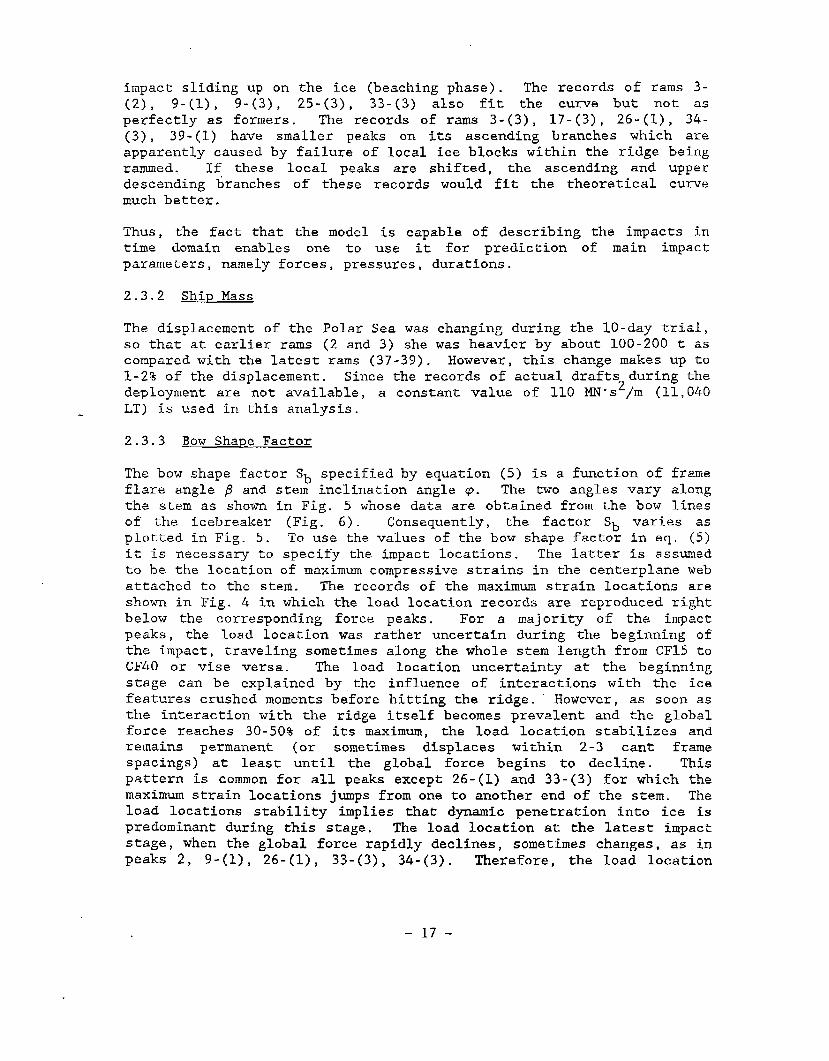
The bow shape factor Sb specified by equation (5) is a function of frameflare angle ~ and stem inclination angle p. The two angles vary alongthe stem as shown in Fig. 5 whose data are obtained from the bow linesof the icebreaker (Fig. 6). Consequently, the factor Sb varies asplotted in Fig. 5. To use the values of the bow shape factor in eq. (5)it is necessary to specify the impact locations. The latter is assumedto be the location of maximum compressive strains in the centerplane webattached to the stem. The records of the maximum strain locations areshow-n in Fig. 4 in which the load location records are reproduced rightbelow the corresponding force peaks. For a majority of the impactpeaks, the load location was rather uncertain during the beginning ofthe impact, traveling sometimes along the whole stem length from CF15 toCF40 or vise versa. The load location uncertainty at the beginningstage can be explained by the influence of interactions with the icefeatures crushed moments before hitting the ridge. However, as soon asthe interaction with the ridge itself becomes prevalent and the globalforce reaches 30-50% of its maximum, the load location stabilizes andremains permanent (or sometimes displaces within 2-3 cant framespacings) at least until the global force begins to decline. Thispattern is common for all peaks except 26-(1) and 33-(3) for which themaximum strain locations jumps from one to another end of the stem. Theload locations stability implies that dynamic penetration into ice ispredominant during this stage. The load location at the latest impactstage, when the global force rapidly declines, sometimes changes, as inpeaks 2, 9-(l), 26-(l), 33-(3), 34-(3). Therefore, the load location
-17-

Y+v32 .- .
30 ,- -
28 ..- -
s26 .- -
6
LM 24
1 ‘
22.
Q*720
18
0
0,5
f3
64 -
60. -
56- -
52-- .
48. .-S&.
4
40~ 7
stations
2 l% 1 1/2 0 -1/2
I II I I
l,, ,,, ,!I / I 1 i I
451
40I i I 1 I
35I I
30I
25 201 ;5. r:
cant framenumbers at the stem J
.;,......;.,
F.P.
Fig, 5 Stem inclination angle “p”, frame. flare angle “~”,
and bpw shape factor Sb along the ship bow length
for the POLAR SEA
–18-

.‘..G
P-1 I I I I In
I 71\ mx\\l\.\P.\.\l \lN I I ~: I
——. ———....-_ ..._. ,. . .
.— .
— ___ ___ +
I. k
w
- x
-\ .—. -. ~,
,.,. .-’\:
+..‘,
..+.
‘,
I
w
-19-

TABLE 2
Global Force Locations & Bow Shape Factors in Accordance with Fig. 4 & 5——— ...
Ram &Peak
1
2
3-(1)3-(2)3-(3)3- (4)9-(1)
9-(3)1415-(1)17-(2)17-(3)25-(3)26-(1)33-(1)33-(3)34-(3)
34- (4)39-(1)
LoadlocationCF #
19
2115-173028-3040
1528392831-3337-3820-282635-3939-15
39-2915
Stemangle
Pdegree
17
17172120.529
1720282022.52718192719
2417
Flareangle
Bdegrees
60.5
62606060.549
5961506158.552626252.562
5759
Bow Shapefactor Sb(Fig. 5)
0.53
0.550.520.670.650.80
0.520.630.790.630.700.780.580.610.780.61
0.740.52
Ichanges for CF40at descendingbranch
1
I
changes fromCF18 to CF40 atthe middle ofthe peak
I
1i
changes fromCF39 to CF15 atthe middle ofthe peak
-20–

corresponding to the upper half of the ascending branch of the peakforce is assumed to be the global force location. The force locationsfor the peaks shown in Fig. 4 are given in Table 2 with correspondingvalues of bow shape factor Sb.
2.3.4 Ice Ridge Shape
Although some of the rammed ridges have been surveyed and profiled attwo or three sections, their shapes are somewhat uncertain and cannot beaccurately described using one or several parameters. Moreover, thelocation and orientation of the ram can hardly be related to aparticular profile. This fact together with the variability of ridgeprofiles, makes it very difficult, if not impossible, to specify theridge shape accurately. Since the structure of equations (l)-(2)depends (though not very significantly) on the ice shapes, a certainidealization of the latter should be assumed. Equations (3)-(5) arederived assuming a rounded profile of a uniform cross-section ridgewhose characteristic size R in equation (5) relates to ridge height.Keeping in mind that any idealization can be rather far from the realridges being rammed, and taking into consideration the relatively lowsensitivity of the total force to ridge shape variations, it is assumedhere that parameter R is specified as:
R =<0.5 (Sail + Keel)but < 8m.4m-R-
When no information on the ridge being rammed is available R = 6m isassumed. The values used in this analysis are given in Table 3 based onthe survey data (see reference 18 of the Report).
TABLE 3
Ram #
239
14-1517
25-2633-39
Site
23
567
# Sail (m)
4.03.4--
3.35.64.8--
Keel (m)
7.06.1.-
9.114.014.4
--
R
5.54.766.28.08.06.0
~ 3/11
1.591.531.631.641.761.761.63
–21–

2.3.5 Dnamic Crushing Strength of Ice
This parameter has not been measured during the tests. Its directrelationship with other strength characteristics of ice (e.g. with thecompressive strength) has not yet been studied. A rough estimate of itsapproximate values can be found in [7, 8] based on analysis oflaboratory tests [2, 3] and ship trials [5]. For autumnal first andsecond-year ice of the Northern Beaufort Sea, the estimate may vary fromA=4 to A=8MPa(s\m3)1/4. Since no particular data onduring the trial are available, a constant value of A = ~;.:(~;;$f)io;:
used for all rams.
2.3.6 Impact Velocities
Equations (l)-(2) are derived considering only that part of the kineticenergy of the ship penetrating into ice which is absorbed by icecrushing, It is associated with the change in the velocity componentnormal to the stem from its initial to final values. The latter is zerounless the ship breaks through the ice ridge. For the horizontaltranslational motion the relationship between the horizontal ship speed“Vk” and her speed component normal to the stem “VR” is obvious (Fig.7):
Vn = Vh Sin ~ (8)
Therefore, the impact force is expressed via the ship speed ,,~hrv
designated as “V” in equations (l)-(2).
Ramming an ice ridge, formed by a number of ice blocks more or lesstightly connected with each other, is a process consisting of one orseveral ice crushing impacts followed by beachings, The ram finisheswhen the ship either breaks through the ridge or is stopped on it andbegins sliding back. When the initial phase (the impact) ends the shipgradually begins beaching up on the ice. The beaching motion iscomposed of translational and pitching motions. The velocity componentnormal to the stem (penetrating velocity) quickly diminishes to zero,and equation (8) is not valid during beaching. The resulting velocityof the ship bow ii~b,,relates to its horizontal component ,!~hrlas follows(Fig. 7):
Vh = Vb Cos (p--y)
where -y- pitching angle (Fig. 7)*-..
(9)
The doppler radar used in the trial was directed to a distant reflector(an ice feature) measuring the horizontal speed only. These measuredspeeds (Fig. 2) can be associated with the impact velocity “V” used inequation (1)-(2) only when no pitching and/or heaving takes place, that
-22-

is at the beginning (or before) of the first impact peak and long afterthe ship broke through the ice ridge. Moreover, since the radar waslocated at the bridge, the bridge’s own rotation due to pitching couldbe a source of significant errors during beachings (Fig. 7). As aresult, intermediate readings might be inappropriate for the impactforce analysis. For these reasons and due to the numerous gaps in thevelocity records, the latter are used in the impact force analysis asfollows. The difference between the initial ramming velocity recordedbefore the first peak and the final velocity of the ram is considered tobe a total velocity loss due to all impacts (distinct peaks) within theram. The velocity losses for each particular impact are estimated bysubstituting the recorded peak forces “F” and durations “T” (Fig. 2)into equation (4) solved for the velocity “V”:
V = 0.1515 TFv/Cos p (lo)
The results of using such procedure to the distinct peaks in the forcerecords are given in Table 4. The total velocity changes calculated foreach ram “Vc” are close to those obtained from the initial and final
readings - “Vr”. For ram 34 it is unclear whether the velocity jump atthe last second of the recorded period should be treated as the finalspeed. Similar question arises for ram 2. The mean Vc/Vr-ratio is1.04.
- “23 -

6
Fig”. 7. Velocity Components at the Stem and the RadarDuring The Impact and Beaching Phases of a Ram
~ _ radar
CG – center of gravity at the impact (CGi) and beaching (CG
Y - pitching angle b) phases
Y“ stem inclination angle
Impact phase velocity components:
Vit – translational (horizontal) velocity
v– normal (penetration) velocityin
Beaching phase velocity components:
v~t.– translational (horizontal)’velocity at the CG
v=o-bn
normal (penetration) velocity at the stem
v– sliding velocitys
‘bh– heaving velocity
vbp
– pitching velocity of the radar
Vr - horizontal velocity recorded by the radar
-24-

T2 16.93- (1) 7.33-(2) 8.653-(3) 9.03-(4) 15.3Total for 3, -
9- (1) ‘ 7.89-(2) 7.89-(3) 14.1Total for 9 -
14 ,16.1
15- (1) I15.015-(2) 4.0Total for 1 -
17- (1)
1
“9.517-(2) 13.817-(3) ~16.5Total for 11 -
25-(1) ~ 8.025-(2)
1
9.225-(3) 19.7Total for 2 -
26-(1) 14.626-(2) 15.0Total for 26 -
33- (1) 15.933-(2) 11.033-(3) 21.0Total for 33 -
34- (1) 6.534-(2) 7.434-(3) 9.834- (4) 14.3Total for 34 -
39-(1) 25.039-(2) 18.8Total for 39 -~~Xion was es
TABLE 4
Peak Velocity changeduration calculated usingfrom equation (10)records Vc;m/s (kn)T, sec
0.660.600.520.920.64
0.510.5*
0.56
0.64
0.660.65*
1.0*
0.600.74
0.7*0.4*
0.77
0.891.1*
0.5*O-4*
0.66
0.55*o.8 *
0.970.50
0.560.5*
mated, an
1.80 (3.50)0.69 (1.35)0.75 (1.47)1.35 (2.62)1.59 (3.09)
~4.23 (8.55)
~:.:; };.;;;
1;25 (2:43)2.57 (4.98)
,1.66 (3.23)
1.70 (3.30)0.42 (0.82)2.12 (4.12)
1.53 (2.98)1.34 (2.60)2.00 (3.90)4,87 (9.48)
0.90 (1.76)0.59 (1.15)2.58 (5.02)4.07 (7.93)
2.06 (4.02)2.66 (5.18)4.72 (9.20)
1.28 (2.49)0.71 (1.38)2.35 (4.58)4.34 (8.45)
0.58 (1.12)0.95 (1.86)1.52 (2.96)1.19 (2.31)4.05 (8.25)
2.22 (4.32)1.52 (2.95)3.74 (7.27>
Recordedvelocitychange foxentire ranv~, h
3.2
8.5
3.7
3.0
5.4
.
8.3
.
7.5
9.0
7.7
9.7/4.0
.
7.5
vc/vr
1.09
1.01
1.35
1.08
0.77
1.14
1.13
1.02
1.07
0.97its lo~atio’nwas assumed to be at CF28
-25–

2.3.7 Impact Forces
The velocities calculated in Table 4 give a reasonable reconstruction ofthe total velocity losses for each ram. With a certain precaution theycan be used as appropriate estimates of the velocities “V” in equation(3). The use of these estimates in equation (3) yields the peak forcesprediction as given in Table 5. Only the peak forces with knownlocation are included in Table 5. The best agreement between thepredicted and recorded vertical forces takes place for the rams with asingle distinct peak force. These are rams 2, 14, 15 for which theratio of predicted-to-recorded vertical forces is, respectively, 0.89,1.01 and 1.39. For rams with several impact peaks the ratio varies moresignificantly (mean value is 1’.06f 0,40).
The peak forces calculated using the estimated speeds shouldconsequently be treated as estimates which might be incorrect forparticular impacts due to the incompleteness, variability anduncertainty of the environmental data (ridge shapes and ice strengthcharacteristics ). For example, the presence of several peaks on theforce record of a ram implies that several consecutive impacts againstseparate (or loosely connected) ice feature took place during the ram.
Constant values of parameters R, A, Sb (characterizing the shape andsize of the ice features and dynamic crushing strength of ice) are usedin analyzing each of the peaks. However, in reality perhaps they variedsignificantly from block to block, Moreover, several rams were donesometimes at the same ridge but at different locations of the ridge(rams 14 and 15 at ridge 5; rams 25 and 26 at ridge 7). The ice datafor these rams might also vary as much as for ridges in differentgeographic areas. These variations can be the sources of the apparentdisagreements between predicted and recorded forces as seen in Table 5for rams 3, 9 (ice data are completely unknown), 17, 25, and 26.
-26–

Table 5
Force Calculated Vertical F talcFn - using Fv=Fncosq Force F recordedequation (10) recorded
MN MN Fv;MN
2 15.78 15.09 16.9 0.893-(1) 4.26 4.08 7.3 0.563-(2) 4.51 4.32 8.65 0.503-(3) 12.88 12.03 9.0 1.343-(4) 15.64 14.65 15.3 0.969-(1) 6.60 5.78 7.8 0.749-(3) 9.65 9.23 14.1 0,6514 17.32 16.28 16.115-(1)
1.0122.44 19.81 15.0 1,32
17-(2) 13.88 13.05 13.8 0.9517-(3) 26.63 24.60 16.5 1.4925-(3) 42.00 38.80 19.7 1.9726-(1) 22.97 21.85 14.6 1.5033-(3) 25.46 22.69 21.034-(3)
1,0814.78 13.98 1981 1.43
34-(4) 12.84 11.73 .14.;3 0.8239-(1) 21.12 20.20 ...~~.(j;: 0.81
-27-

THIS PAGE INTENTION.4LLY LEFT BLANK
-28-

THIS PAGE INTENTIONALLY LEFT BLANK
-29_

3. HULL STRUCTURAL RESPONSE
3.1 Method of Analysis
The dynamic structural analysis was perform- for the vessel ramming in iceat a head-on condition. This predicates a condition of symmetry about thecenterline plane of the vessel, allowing the analysis to be performed on a modelrepresenting only one half of the ship, in this case the port side. NO lateralor torsional response of the vessel was considered since the ice impact loadsare expect< to be approximately symmetric with respect to the centerline planeof the ship, and the lateral and torsional response is assumed to be insignif-icant.
The mathematical model has a fairly fine distribution of elements forward,and a much coaser distribution aft, with a smooth transition in between. ThiSwas done so that the dynamic response in the bow and fore body of the vesselcould be determined with a reasonable degree of accuracy, while still providinga good representation of the stiffness and inertia characteristics of the entirevessel. An accurate representation of the hull girder structure is reflected inthe calculation of the natural frequencies and mode shapes of thethree–dimensional model.
The static characteristics of the vessel afloat were determined by using theABS/SHIPMOM program for the calculation of the buoyancy springs. The outputfrom SHIPMOM program was then used to determine the dynamic characteristics ofthe vessel for the calculation of added mass with the aid of the ABS/ADDMASSprogram, which is bas~ on the linearizd ideal fluid theory and the use of theboundary integral method.
,...The global ice impact loads for the vessel were determined bas~ on the load
analysis presented in the preceding sections. The effects of internal andhydrodynamic damping were introduced in the pertinent calculations of structuralresponse.
The free vibration characteristics and the dynamic responseical model to the ice impact loads were calculat~ by means ofgram. Details of the various steps, processes and aalculationifollowing sections.
of the mathemat–the SAP-V pro-are given in the .
-30-
3.2 Mathematical Mcdeling
3.2.1 Three-dimensional Finite Element Mcdel
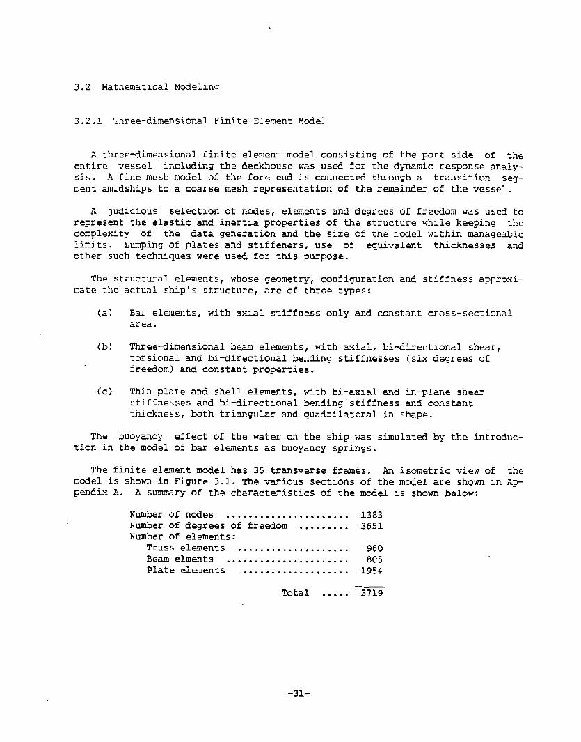
A three-dimensional finite element model consisting of the port side of theentire vessel including the deckhouse was us~ for the dynamic response analy-sis. A fine mesh mtiel of the fore end is connectd through a transition seg-ment amidships to a coarse mesh representation of the remainder of the vessel.
A judicious selection of ncdes, elwnents and degrees of freedom was used torepresent the elastic and inertia properties of the structure while keeping thecomplexity of the data generation and the size of the model within manageablelimits. Lumping of plates and stiffeners, use of equivalent thicknesses andother such techniques were used for this purpose.
The structural elements, whose geometry, configuration and stiffness approxi-mate the actual ship’s structure, are of three types:
(a) Bar elements, with axial stiffness only and constant cross-sectionalarea.
(b) Three-dimensional beam elements, with axial, hi-directional shear,torsional and hi–directional bending stiffnesses (six degrees offreedom) and constant properties.
(c) Thin plate and shell elements, with hi-axial and in–plane shearstiffnesses and hi-directional bending”stiffness and constantthickness, both triangular and quadrilateral in shape.
The buoyancy effect of the water on the ship was simulated by the introduc-tion in the model of bar elements as buoyancy springs.
The finite element mdel has 35 transverse frames. An isometric view of themodel is shown in Figure 3.1. The various sections of the model are shown in Ap-pendix A. A summary of the characteristics of the tiel is shown below:
Number ofndes ...................... 1383Number<of degrees of freedom .● ....... 3651Number of elements:
Truss elaments .................... 960Beam elments ...................... 805Plate elements ................... 1954
Total ..... 3719
-31-

-32-

3.2.2 Buoyancy Springs
The effect of buoyancy of the water on the ship was sirnulatdvertical springs whose stiffnesses are equivalent to the buoyancy
by introducingeffects at the
corresponding ship stations. Each node located along the wetted surface of theship connects to an axial bar, acting as a column, which is the equivalent ofthe buoyancy spring.
The equivalent vertical buoyancy stiffness at a ship station for a givendraft is the vertical force necessary to produce a unit vertical deflection atthat station. This stiffness can be expressed as
K= pBS
where
P = density of waterB = breadth of ship at waterlines = station spacing
The stiffness of an,axial bar acting as a column is given by
K’ = AE/L
whereA= cross-sectional area of the barE = modulus of elasticity of the barL = length of the bar
Equating the two stiffnesses, we get
,..A= PBSL/E
All values of L are conveniently chosen as 24 inches in this study, and themodulus of elasticity of the bars chosen to match the modulus of elasticity ofthe ship structure, i.e., E= 29. x 10’ psi.
The cross-sectional area obtain~ from ahve is the total equivalent area ata ship station. This area is then distribut- to the various nties in contactwith water, in approximate proportion to an effective transverse width associ–ated with each node.
Table 3.1 shows the calculation of the equivalent areas of the buoyancysprings at the 35 stations of the mathematical xdel.
-33-

Table 3.1 Calculation Of Buoyancy Springs
Mdel Ship Spacing W.L. Beam Area (whole ship)Fr. No. Fr. No. (in) (in) (in**2 x 1O**-5)
1
23456789101112131415161718192021222324252627282930
+- 31..32333435
2752632532432332232111971821711561431281131009285786957
CF-75CF-69CF-64CF-56CF-51CF-45CF-41CF-37CF-33CF-29CF-25CF-21CF-16CF-11CF- 6
96.00184.0016a.24160.20160.08176.04208.08232.08208.08208.08223.92223.92240.00223.92168.00120.00112.08127.92168.00120.0072.0088.08103.92104.7682.0875.7269.6068.8868.8868.6467.5678.2488.08124.2080.40
0.00146.04321.00466.80578.52664.44742.08814.08861.48887.28909.96925.32943.68949.20946.32938.16926.04908.64874.80807.24785.76737.40691.80605.44545.76477.72416.88351.00279.72202.20138.1284.000.000.000.00
0.005.7211.5015.9019.7024.9032.9039.9038.2039.3043.4044.1048.2045.2033.8024.0022.1024.7031.3020.6012.0013.8015.3013.509.547.706.185.144.102.95“1.991.400.000.000.00
-34-

3.2.3 Boundary Conditions
The finite element model is supported vertically by the buoyancy springs atthe various nodes in contact with water.
Along the centerline plane of the model, appropriate boundary conditions arerequired to account for the symmetric response, since only the port half of thehull structure wasalong the centerline
Ux = O, zero6y = O, zero6’Z= O, zero
At the aft end, asupport the model
modell~. Namely, the degrees of freedom for all the nodesplane should be specfied as follows:
transverse displacementrotation almut the vertical axisrotation abut the longitudinal axis
spring with an arbitrary small stiffness value was used tolongitudinally, thus providing another necessary constraint
for a statically stable mathematical model.
3.2.4 Loading Conditions
A total lightship, cargo and miscellaneous weight of 11,200 LT was includedin the finite element model. This weight of 11,200 LT was the gross weight ob–tained by excluding 1859 LT of fuel used by vessel to get to the ice fields fromthe departing gross weight of 13,059 LT.
The concentrated loads of major machinery items and other equipment were di-rectly lumped at the adjacent ncdes. The masses corresponding to the cargo,fresh and drinking water, fuel oil and lubricant oil were distribute to thevarious rides in the load~. area. The structural weight was taken into accountby specifying a material density of the mdel that would result in the desir~total lightship weight.
3.2.5 Hydrti~amic Add& Mass
As the ship is vibrating, the hydrtiynamic forces acting on the ship hullproduce an effect equivalent to a very considerable increase in the the mass ofship, known as “added mass.” In ship vibration analysis, the added mass shouldbe properly taken into account since it is the same order of magnitude as themass of the sh,ip.
The added mass distributions were calculated for a draft of 28 feet by theABS/ADDMASS program, which was developed based on the linearizd ideal fluidtheory, using the tiundary integral methd. The underwater hull geometry is ap-
-35-
proximate by contour lines at 35 longitudinal stations. Each contour line isrepresented by line segments, on which added mass contribution is found. Thismass is then lumpd at the corresponding ndal points of the finite elementmodel in contact with water.
It is noted that the addd mass calculated is the vertical component result–ing from heaving oscillation only. No transverse and longitudinal componentswere included since lateral vibrations were not considerti in the analysis andthe longitudinal added mass is considered negligible in this case. The lumpedvalues of the added mass for the 35 stations of the finite element mcdel areshown in Table 3.2. The total values of the added mass in the vertical direc–tion was found to be 63966 lb-sec2/in. which is equal to 98 percent of the totaldisplacement of the loaded vessel.
3.2.6 Damping
The damping associated withthe combination of the following:
ship hull vibration is generally considered as
(a)(b)(c)(d)(e)
Structural dampingCargo dampingWater frictionPressure waves generationSurface waves generation.
The formulation of expression for the damping forces poses a difficult prob-lem that still requires extensive research. For practical purposes, however, itis assumed that the effects due to structural damping, water damping, waterfriction and pressure waves generation can be lumpd together and the effect ofsurface waves generation can be neglect~.
In this analysis, a damping value equal to 5 percent of critical damping wasused. This value was divided into two factors proportional to the mass andstiffness matrices for use in the SAP–V program. The form of Rayleigh damping .is:
[c] =a[M]+D [K]
where[c] = damping matrix[M] = mass matrix[K] = stiffness matrix
a = mass-proportional damping factor6 = stiffness-proportionaldamping factor
For a single mde response, the relation betwem the dmping ratio and thetwo damping factors can be expressed as:
-36-

Table 3.2 Hydrodynamic Added Mass
Model Ship Spacing W.L. Beam M (whole ship)Fr. Ho. Fr. No. (in) (in) (lb-sec**2/in.)
123456789
1011121314151617181920212223242526272829303132333435
2752632532432332232111971821711561431281131009285786957
CF-75CF-69CF-64CF-56CF-51CF-45CF-41CF-37CF–33CF-29CF-25CF-21CF-16CF-11CF- 6
96.00184.00168.24160.20160.08176.04208.08232.08208.08208.08223.92223.92240.00223.92168.00120.00112.08127.92168.00120.0072.0088.08103.92104.7682.0875.7269.6068.8868.8868.6467.5678.2488.08124.2080.40
0.00146.04321.00466.80578.52664.44742.08814.08861.48887.28909.96925.32943.68949.20946.32938.16926.04908.64874.80807.24785.76737.40691.80605.44545.76477.72416.88351.00279.72202.20138.1284.000.000.000.00
0.0083.30374.31787.311258.601820.102724.003689.303911.804361.805180.005496.406153.005678.204151.702874.402550.502714.903116.301727.20958.111009.201031.00804.94511.23365.25250.91178.92109.3257.1826.3110.760.000.000.00
Total 63966.25
-37-

It is assumed that one half of the damping ratio is mass-dependent and theother half is stiffness-dependent. The a and 6 damping factors were calculat~for the ratio of critical damping { equals to 0.05. With the frequency u of19.2 rad/sec (3.06 Hz) which corresponds to the two nde bending mode of thehull girder, the a and p damping factors were found to be 0.9605 and 0.0026 re-spectively.
-38-

3.3 Free Vibration Analysis
The finite element mcdel with 3651 degrees of freedom representing the hullstructure has the same number of natural frequencies and corresponding retieshapes, which may be obtained by solving the generaliz~ eigenvalue problem re–presentd by the equation :
[K]{#} =
where[K] =[M] ={d} =u=
symmetrical square stiffness matrixdiagonal mass matrixcolumn retieshape matrixnatural frequency
This problem of free vibration was solved by means of the SAP–V computer pro-gram using a subspace iteration solution.
The lowest 10 modes of the vibration of the ship hull for the specified draftof 28 feet have the following characteristics :
---——- --.---— -——---- -----—— --—--- ------ ______ ______ ______ ------ ______
MODE NATURAL FREQUENCY PERIOD REMAXRSNo. (Hz) (See)----—- --—---—---—----__________..__-_____ ______ _____ _______ -----_____
1 0.02 62.29 Rigid Btiy Surge2 0.45 2.21 Rigid Bmly Heave3 0.50 1.99 Rigid 13dy Pitch4 3.06 0.33 2-Node Bending5 5.54 0.18 3–Node Bending6 7.75 0.13 4-N@e Bending7 9.81 0.10 5-Node Bending8 10.20 0.098 Deckhouse9 11.86 0.084
10 12.60 0.079-——--- ------ ----—---__-—--_—-- ____________ ______ ______ _______ _______ _
The rnde shapes corresponding to the tive 10 reties are shown in Figure 3.2.
The same scale was us~ for the internally orthonormalized eigenvectors.
It can be seen from these plots that the first three reties represent therigid My motions, namely, surge, heave and pitch. The remaining mcdes repre–sent the elastic deformations.
-39-

I
in
1%2co
m●
m
-40-

Mode 3 - Pitch
Mode 4 - 2-Node Bending (3=06 Hz)
m. B
Figure 3.2 Vibration Mode Shapes (continued)

I
mI
-54J
i?-1u
u
-42-

Mode 7 - 5-Node Bending (9.81 Hz)
Mode 8 - Deckhouse (10.20 Hz)
Figure 3.2 Vibration Mode Shapes (continued)

I
m
w
10al
Q
m.
(-’-l
b-dk
u
-44-

The lower elastic modes, fourth to seventh modes, correspond basically to thehull girder’s 2–node to 5-ride vertical bending vibrations. The higher m~es in-
dicate hull girder vibration coupled with deckhouse and local vibrations andmust be understood as representing the response of a three-dimensional finiteelement model as opposed to the usual free-free beam representation of the ship.
–45-

3.4 Dynamic Structural Analysis
3.4.1 Problem Formulation
The finite element model of the vessel is subject to time varying loads which
represent the impact loads induced by ramming multi–year ice.
The dynamic response is obtained by applying the time varying bow forces to
the model and solving the resulting dynamic problem given by the followingequations of motion.
[M]{ti(t)] + [C]{;(t)] + [K]{u(t)} = {F(t)}
where[C] = damping matrix{~} = column matrix of accelerations{u] = column matrix of velocities{u} = column matrix of displacm”ent${F] = column matrix of applied forces
The structural response to this impact loads is of transient in nature. Re-sponse time histories for selected n~al displacements and element stresses ofinterest can be obtained. The problem was solved by the SAP-V computer programusing direct integration by the Wilson 8-method, which is unconditionally stable[9].
-46-

3.4.2 Ice Impact Loads
Ice impact loads applid to the structure were represent by time varyingloads. In the present study, calculations using different forcing functionswere performed first for purposes of comparing the dynamic response of the hullstructure. A total of nine loadcases were selected for the dynamic analysis:
Load case 1
Load case 2
Load case 3
Load case 4
Load case 5
Load case 6
Load case 7
Load case 8
Load case 9
Triangular shapeLoad at location A between cant frames 21 and 25Concave trigonometric curveLoad at location A between cant fremes 21 and 25Convex trigonometric curveLoad at location A between cant frames 21 and 25AX theoretical bow force curveLoad at location A between cant frames 21 and 25Ram 39 measur~ bow forceLoad at location A between cant frames 21 and 25Ram 39 measur~ hw forceLoad at location B between cant frames 41 and 45Ram 39 measured bow forceMoving load from location A to location CRam 14 measured lmw forceLoad at location D between cant frames 25 and 29Ram 14 measured bow forceLoad at location C between cant frames 33 and 37
The first three cases were based on predefine forcing functions as shown inFigure 3.3. For these forcing functions, the total duration of the load was as–sumed to be 1 second. The time to reach the peak value was chosen to be at0.667 second. The peak value of the unit impact loads was assumed to be 2 MN(449 kips).
The time function for load case 1 corresponds to a triangular shape and thatfor load cases 2 and 3 has a distribution in the form of concave and convextrigonometric curves,respectively. The area under the load time history curverepresents the energy content of the impact load. By having the three shapes offorcing function as defind akmvef it is anticipated that as compar~ to loadcase 1, load case 3 has a higher energy content of impact whereas load case 2has a lower energy content.
Load case 4 uses the ABS analytical kmw force history curve shown in Figure3.4. Similar to the first three cases, the duration of the impact load wastaken as 1 second. However, the time to reach the peak force in this case was0.728 second and the peak value of kaw force was assumed to be 2 MN.
Based on the measured time histories of bw forces, it was not~ that in eachof the ramming tests, there were several waves of impact during the measurdtime of 25 seconds, Each rise and fall of the force was considerd to be a waveof impact. Frau the measured data, the time duration of impact was atx)ut1 sec-ond for the first wave of impact before the next wave of impact. Consequently,
-47-

Figure 3.3 Predefine forcing functions forload cases 1, 2 and 3
-48-
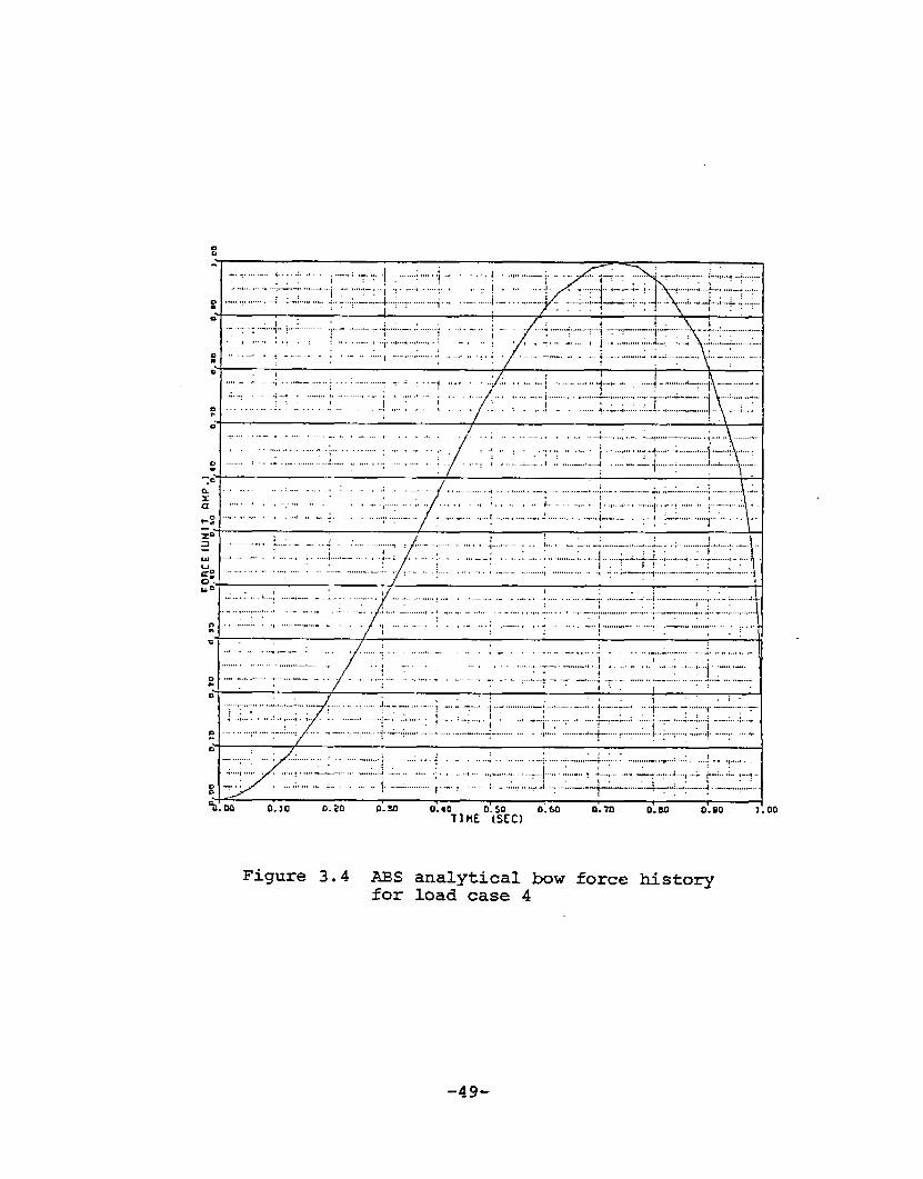
Figure 3.4 AllS analytical bow force historyfor load case 4

in the ative four case studiesf only one wave of impact having a duration of 1second was considered. The force level was maintained at zero at the end of the1 second impacts and the analysis was carried out for additional 2 seconds toobtain the dynamic response of the structure after the impact ended. The lo-cation of the impact lmw forces for all four load cases was assumed to be at be-tween cant frames 21 and 25 and designated as location A in Figure 3.5. Thetotal load was evenly distributed into 5 nodal points along the center line inthe finite element model.
In the second category, the dynamic response was obtained using the acutalbow force time histories recorded during the ice–impact tests of the polar sea.Two cases, namely, Ram 14 and Ram 39 were considered in this study. Ram 39 waschosen in the analysis because it has the highest peak value of the lmw forceamong the 40 rams recorded. Furthermorer the bow force time history indicatesthat a peak force of 25 MN occurs at the first wave of impact following imme-diately with very small values of subsequent waves. Other rams showed that thepeak bow forces often did not occur in the first wave impact and if it did oc-cur, the peak forces were much lower in magnitude.
For each ramming, the total duration for the bow force meas~rement was 25
seconds. However, due to the SAP-V program limitation, the dynamic analysis wasperformed for the initial 3 to 5 seconds only, depending on the size of thetime–step used in the analysis.
Using Ram 39 data, three load cases were performed with different locationsof the application of the lmw force. The location of hw force for load case 5was the same as in the previous load cases (location A) whereas the location forload case 6 was between cant frames 41 to 45, designatd as location B in Figure3.5. Load case 7 uses a moving load. Initially, the location of the bow forcewas between cant frames 21 to 25 and the load moved during the loading process.The velocity of the impact load was taken as 4.4 m/see. The duration of themoving load was 1.2 seconds such that the final position of the load ended be-tween cant frames 33 and 37 (location C in Figure 3.5).
For load cases 5 and 6, the analysis was carried out for 300 time steps witha timestep size of 0.016 second for a total of 4.8 seconds. During the initial2.4 seconds, the bow force followd the shape the record between 5.6 to 8.0 sec-ond for - 39. After that, the load was held constant at 14 MN for another 2.4seconds period.
AS tbr load case 7, the moving hw force lasted for 1.2 seconds. After the.>initial 1.2 seconds, the load was held at a constant value of 7 MN and was ap-plied stationarily at location C for another 1.8 seconds (see Figure 3.6). Thetotal number.of time steps used in this loadcase was 300 steps with a step sizeof 0.01 second. The reason for allowing the moving load to stop at location Cwas again due to the limiation of SAP-V program capacity. Nevertheless, thiswould not affect the analysis as the maximum peak stress was expect~ to occurat a time instant of abut 0.85 seconds and was well within the initial peridof 1.2 seconds.
The next two loadcases were carried out using ~ 14 &w force time historyrecord with two different locations of load application. The location for load
-50-

case 8 was at location D between cant frames 25 to 29 and for load case 9 was atlocation C (Figure 3.5). The initial 2 seconds of the load was taken between13.0 to 15.0 second of the time history shown in Figure 3.7. The analysis wascarried out for 300 steps using a time step size of 0.016 second for a4.8 seconds. Ram 14 was considerd as a good ram without inducing amotion. The maximum bow force peak value was 16.1 MN and the forceconstant at 6 MN after initial 2 seconds.
total ofbeachingwas kept
-51-

,.. ”
Jlh)I
Y
‘“ “’-/7-+’ “’-r”
ion
I
u Location A
Location Dc
Figure 3,5 Forward end of Center line keel showinalocations of applied bow force
A

t-
l“” 1’”
{
.- . . .
——
wWI
0
. .
L.
}
. . .Ir
.
3W
%-
‘\...... mu-l
. .
s.; v-l
x“ J In. . .. .
mu+-
.H
cwu-l
,.. . . . . .
L ,,, !,. ,,l,.l, 1,.,, t I,.,.,q

w
-1JId
m
Wa)tordc)
-dI
. . . .
. .
..
u-lv-l0
. .
. .
.
.
. .
@“-k::. . . . . . . . .-
. 0
..-. . . m 2.—
.
. . .+
.
.. .
. . .
.
. Im.“ru
1-.m.
.LVmm
.
.

3.5 Discussion of Results
The dynamic response in terms ofments along the side of the 01 deck3.8). The stress time historiesstrain gage locations are present~
stress time history was obtained for 31 ele-over the entire ship length (see Figurefor 9 select~ elements corresponding to thein Figures 3.9 to 3.17 for all the various
load cases consider~. To better evaluate the response of the vessel, the dis-placement time histories for 7 select~ ndal points along the center line of 01deck are also presentd in Figures 3.18 and 3.19 for two load cases.
As can be seen from the stress time history response curves, the peak stressand the time instant at which the peak stress occurs are of primary concern.Tables 3.3 to 3.11 show the values of the peak stresses and the correspondingtime instants for all the selected elements on the 01 deck. The strain gage lo-cations related to the element number of the mathematical model are also listedin the tables. A surmnaryof results for the 9 load cases considered is given inTable 3.12.
In the polar sea ice impact tests, the direct measurements were made in termsof the strain time hisotry. These strain time history data were then convertedto stress time history for all the strain gage locations to obtain the verticalbow force time history of the ice load. The present analysis is a reverse proc-ess. Using the interpreted ice loads, a dynamic transient analysis was per-formed on the finite element mdel to obtain the response in terms of stresstime history. A comparison is made of the calculatd and measured results.
Before using the actual ice load time histories provided by ARCTEC, four loadcases using predefine shape of time function for unit ice loads were used inthe analysis. The maximum vertical baw force of these unit loads applied tostrcuture was taken as 2 MN.
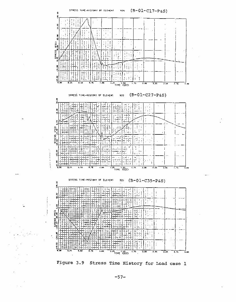
Figure 3.9 shows the results of stress time history corresponding to loadcase 1, which has a triangular distribution of time function. The maximum peakstress was found to occur at element 914 (B-01-39-P&S) and has a compressivestress value of 610 psi at the time instant of 0.68 second. The stress responsecurves follow closely to the shape of the applied load time history and the phe-nomenon was more distinct at the locations such as elamants 919 (B-01-C35–P&S)and 921(B-01-C27-P&S) in way of the frames where the lmw force was appli~. Inaddition, hull girder vibration effect was observd near the midship region.This vibration effect can be seen from the stress time history of element 906(B-01-128-P&S).
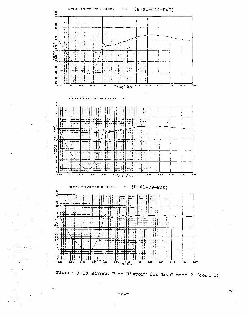
The effect of dynamic response as describ~ above is more obvious in loadcases 2 and 3 in which the forcing function is in the form of trigonometricfunctions. Referring to the stress time history of element 906 in Figure 3.10for load case 2 and Figure 3.11 for load case 3, it can be seen that the dynamicbehaviour is similar to the bending stress time history for gage BO1-128-S ofRam 9 given in the ARCTEC Report. The frequency of vibration as noted in thestress time histories is 3.06 Hz, which corresponds to the frequency of thetwo-ncde bending mode of the hull girder. The two-node banding vibration isseen to be more pronounc~ amidship and becomes less and less distinct towards
-55-

-..
.. +.
(S5d-6E-10-H)
(S~d-SS-TO-EI)
(S9d-98-10-~)
(S9d-8ZI-10-Q)
Lz6\926. “-----S26PZ6EZ6ZZ61260266168T6L169T6ST6
/z8E-c
606—
H
!ijll
806 — /’ ./’”,/’
Lo6–/’//! / ’68’
U_u“1’206 —
Z06—
106-
006 —
668 —
868—
L68 ~~~wq
-1
0
m
m●
m
-56-
. .
51 R[5S llM[. HIS IORr or [L IHEM1 ~w (B-01 -C17-P&S)
_TT-———.———.‘~.,,.— —.,.-,,.,,,
:!! . . . .,!,;;; 7-’ !
-;’r ‘,,.!,...—... .
? ‘!! ;,
,,. ,., i.. ,,!;!!: {.~~i l:;,
;4 .,,.!; ~ ~:-!i .:: :,,
,,‘/J: !;;:,, :.,
F! 1.s0 1.7s >lIME ISECI
. . .
-—
I I
l!““-~ i
I----. / , ~~
I
.-—. .1 _
/
-.,.,...
Ib ?.50 >
STRESS llHE-til S15RY OF ELEHEI+I .ZZ (B-01-C27-P&S)
-=-
.
?5
I
)
.. .
:. .- -
k
I. . —
.... ,-.
. . .
75
00
m
..”.
5TrIESS TII+E-HIS1ORT OF ELEHENT
s9ZI (B-01 -C35-P&S)
e.
,,..
I
.,. . . . . .... . . .
Figure 3.9 Stress Time History
-57-
for Load case 1

I
. ..-:
. . .. .,-.
.. . ..., -..
51RES5 llM[.Hls]np,~r [~~”~~, 919 (B-01-c44-P@
,:! ii,. !
!l~: .:
~ L.! ; : “, 1 I
i ; :,,.
- —. .-—— _ ..__ __,,.,!,
>;
.:,; . .
l-~ .,,4, , I-i~l : 1~ —J-–—– .1—---- I ;
STnESS llHE-ttl SIORT OF [LEIIEIIT 911
s
I-;-1>+<. L-. :,...
— -1-4 ;-—..;–.. ; ‘--==4
I
. .
I1
1-’-’””
‘o. m 0.2s 0.50 0.’25 1.00 );>s 1:50 1:75 2.00 2.25 ?:s0 ‘——?.7s 3.DUlIHI ISECJ
ST~ESS lIHE-HISIWIT or EL EHENT 9111 (B-01-39-p&S)E
I----- I –.. .—
——.. -—.—,,,.
.-.. ,. .-. ..-
. . . . --- ._.-
Figure 3.9 Stress Time Histo~ for Load case1 (cent’d)
-58-
,.. ,. . ...’

.
....
.,,.. .... ,,.-..-.
,.
STRESS llH[-HISlflFII OF [L IHFN1 913 (B-01-55-P&s)
mlmE
.
a
I-l—-,- ,
; ,...
SIRLSS 1IHE-HIS1ORT OF ELEMENT gcm (B-01-86-P&S)
,, ,1,,,1,, .i, .,
STRESS TIME -H IS1OR7 OF ELEHENT 9DS (B-01-128-P&S)s
Figure 3.9 Stress
,.:.--...,,.+..’:’.,........>..-.,., ,
Time History
-59-
m ::7s,..,,-:
... -—
j--, 1,..
I
..-
.
. . _-
.-—.. .
;., ....
--.,. ,.
—..-
;.—.....-
.-..
-.—.—
T--n
Eu
fl
for Load case
!..,,..-——-.....*
3.05
1 (cent’d)

4—.-..----.....-—-—.i..->--—,—-.,.,;,:.,.-—-.,,’,:.r
.- 1 iI
.-... ~. I
1......
‘1 i
--.=.,<
SIMSS lIHE-HISTOR7 or ELLHEMT 9z2 (B-01-C27-P&S)
-.
_.x...!’”-““:-..%..-,/’
-b—---...-,,:....!”
,.,
!+__-../...-,i ‘1 \_____ ... . .;, ”,.: ~
.;,I
! .
!
. .
. . .
I
m >.25 2.5D 2.75
5T~ESS TIHE-HISIOFIr or CLEMENT SZI (B-01 -C35-P&S)
m
00
,,
Figure 3.10 Stress Time History for Load case 2
-60-
. . ,,,..,:,,,
.-.
SIRLSS 1 IME-HISIDFIT Or EL EHEN1 911
s
., : I I
.-
-.-A--
,.,. . .. .
. .-
1. . . ...1
‘0.00 n.?=? 0’.50 0;75 1.00 1:25 7.50 ):75 2:00 ::2< ?“.50 2’,75TIHE [SEC)
SlnE5s TlmE-H1510R7 OF ELFHEWT 9,V (B-ol-39-P&s)
‘o.m 0;2s tin.* 0:+5 “- l“.m 1:2! 1:s0 8;7s1I HE ISEC)
2.m
_,.:,,
I
i——-—! . . .
I
~...
il..
— ...!— -:
1—. + . . . .
;’
1’—- 1. .. . .. .
-1
i
so 7.w s.m
Figure 3.10 Stress Time History for Load case 2 (cent’d)
,----
,-’,.-
-61--.: ‘.::.?..-.>.
. . .

sIR[ss llH[.1.llsl~RT O( [L EHEM1 913 (B-ol-55-P&s)
....
. . ..-.. .. . .
.....,.,.
‘ L-l
:.,,, ,,ij
:!’ ,!::.,! .,,,
— .— -.
lIM[
=-l--1
1:II
— .—. —-,. < .._ ,
.,, Ii1’
~—.._ .
;1: ,:;,, , i,, ,,
-- .—.
STRESS lIHI.HIS.l DRT DT ELEIWU1 909 (B-01-86-P&S~= .,, ,,...,,. ,, 3
:! :1,: !11.~
4!!!1’1 .!l
---- —-.
~! ’!’’!’’”!w “ J +--”..~ .: . . . . . .
SrR[5S llHE-HISIOn T Or ELEHENT 922 (B-01-C27-P&S)E
:>m.Y.. ----r,,., :..-..>J,. —
I .,, !,,!, ,,, .,..:,, ,, !,..,,! !,
?O,.m ~,..., ~,.=n1 1
0.7s l.m 1.25 1.s0 1.?5 ?.m 2.?s 2.s0 ?. 75TIHE (SEC]
—.
STRESS TIHE-HIslbnY OF ELEtiENl 9.?1 ,, (B-01 -C35-P&S)=
Do
1!1.-,
;l..
“: !—..,.,:,.
:-!:.
-..{-;.
:.
-..:!:I;f“’.—.,,~
i“1!,.
5 3.00
Figure 3.11 stress Time History for Load case 3
’63-

I
i
.,
.-
l)HC IsLC}
51 FIESS lIHE-HISIDRT OF ELCHEMT 917
:
II
-L__!-–.-1...
L—.....—
r——
—. .—..... .,:.
,,,—--- -....—
J,,
,,
— —.. — .—
‘1Ill
>j
m ?.7s 2.50 ?
.—. .
——
—.
n
STRESS 1IHE-FIIS1OBT Or ELEHEt17 91V (B-ol-39-P&”s)
11 KE tsECl
00
Figure 3.11 Stress Time History
-64-
for Load
,,,,— ......—.
,..,,~:i
.~.~;.:!
—- .-!,.-
! .;1.!,.
I _,,—-
1 {i!~ ,l!”;
.;,
! ‘i
50 2.?s 3.m
3 (cent’d)

STRESS llHC-HISl@Q! mf EL FMEU1 913 (B-01-55-P&S)
1
;- 11
— —----- I .{ I:>;
( /
- ... =— — -_ I__
‘-; lq
;i. ” .:
1’ ,: ,
1.:., ,. . ... .—. - .——
-’-{-p).i ~“; ; :.:!; ! .!
—..1.–-.. . . . . . ----“-r-
$:1 .1 ::,+.!.. ! -~.~ i.
II.
1’
~ -i. – ;2 :> I .__...—
j;++ . .:.;. : ! !,,
i.!::;. ;-:.; ; “!: 1.Y : . .
M 1.?5 ?.m ?.?sSEC)
?.s0 >.15 3,00
SIFICSS. llH1-141S1DRT or ELEMEW 909 (B-ol-86-P&s):,
,., ,,, ,“km 0.25 0.50 0.% I.m 1.>5 Is@ 1.7s ?.QO
I)ME ISEII?.2> >.>0 ?.75
S1RES5 TIHE-HISIURT, OF EL EHEU1 906 (B-01-128-P&S):
m
Figure 3.11 Stress Time History for Load case 3 (conk’d)
-65-
,

51 H[S5 II H(-HISIDM1 01 [Lt HfNl 92ti (B-01-C17-P&S)
II,!’
—. A
r
,,I,,,
,’—!:
:1!,
,\ ,’,1,
,1!’;:1.
~.;1,,;, ;
r
--- ,__ i__~-_,
..—__,.._.._..,
T
1,——-—-—--------j!,.— —. ---.—..—.,.;,,:.1.;,:m ?.25
~?.s0 2.>5
SIRESS I1HE-HIS1ORT OF ELEHEN1 922 (B-01-C27-P&S)
5~fl[55 ~ lHF-Hl.51DR~ OF ELEHEN; 921 (B-01 -C35-P&S)
w
m
Figure 3.12 Stress
! .!;
‘“l”’.—-.,.:;,,:-.~ ,,.;.::—..;,..
j:,,/,.,-i..‘ :
-:;,.,
:,,,,::
d—.,; . . .
so 2. 7s 3.00
Time History for Load case
-66-

SIRESS 1IH[-I’IIS1ORI or [L CHFU1 ~1~ (B-01 -C44-P&S)=
lIH[ 15tcl ‘“
SIHISS 71n[-HISIORr of EL EHEN1 917
:
. —-- .,. . ._. -
. .——. -------
;;:.
..; , .;l.; .,, -., ,
;.4
,’ ,,- —. —.
ili~ :’”:. ,.
~.,— .-L-.......—..,,.;.!;: ‘
w 2.25 2.50
..- --
-
——,
——.
75
STRESS lIHE.MISIDBT OF [LEHEMT 91q (J3-ol-39-P&s)
1I HE ISEC)
-—
..---—
m
.00
Figure 3.12 Stress Time History for Load case
-67-
4 (cent’d)

$I~(5S II HI-}! IS IDHI Of iLEni Nl 913 (B-01-55-P&S)
.,— -—. _
j~~.—-—-.—-——, .
!
-.. .—.— ,----- .—-..
,4,
-- 1‘.. /
l;. :–y --!.. ,
“: I..-—...-—:.’:
~:~ “’
.- —- —— .--— .
!.,”;: .; :.:,—.: ,:!
m 2.2\ 2.50 ?.75 3,00
s1RE55 11~~-~tsln,qr of EL EHEH1 909 (B-ol-86-P&s)
+
1
-——,,,
!:
.,
J,
1~~w
,’
7——.,,,,,.,...—.l-=-1’
w 2.?$ 3.00
slncss TIME. HI.51 DRY Or ELEHENT 905
:
(B-01-128-P&S)
.
Figure
0.50
3.12 Stress Time History for Load case
-68-
4 (cent’d)

. .
,.,.
..-
.,,
.,
51hES5 llmf-nl~lohl UI L~tmtml 92q (B-01-C17-P&S)2
.
SIM35 1IHI-HI$1OR1 OF EL KHEH1 922 (B-01-C27-P&S)=
STRESS TIHE-H151ORT OF ELEHEW 921 (B-01-C35-P&S)
Figure 3.13,. ..
Time History for Load case 5
.,. .-69-

1 IFIC ISECI
SIBE5S llnE-li151bE. r IV fLEHENT 911
:
-.
S?nE5S I lHE-HISTDnT OF ELEPIEU1 91V (B-01-39-P&S):
Figure 3.13 Stress Time History
-70-
for
1:..-.!;
~:——,.:.
---—
/“ ,.
. . .&-
,,.,,.!
-—-::,
;,
i.
m ● .DO
case 5 (cent’d)

. . .-- —-.
..
! 11”1’.11.,:I I:;:,\;~:;),’,, ‘1.;, :, ,’1i
SIHESS liHF-HIslbRl OF ELEMENT 909 (B-01-86-P&S)=
8
—...-
sTRE5s 1 lnl-HISIDfi T of EL EHEN1 9D6 (B-01-128-P&S)
.’-.’”:...;;,,,.:,=:... “-.” :.. .- .:,
. . . ...
. .... ... ..,”.
.. ,.,
m
i
Figure 3.13 Stress Time History
-71-
for Load case 5 (cent’d)
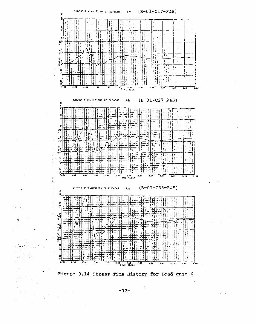
$IRCS5 llHf-M151rIh T Of iLth[Ul 92U (B-01-C17-P&S)
.-
STRESS 71 HE-H IS] Ofi~ OF ELE”EHT 921 (B-bl-C35-P&S)=
.,. ... ---. .
i
. ...-.
. .. .+
,,... ...
..- _
;:.—--,
!,
) BO
●
Figure 3.14 Stress Time History for Load case 6
-72-,,

slmss IIML-HIE.IwII nf [[[HEW 919 (B-01-C44-P&S)s
.....
—,
. . .,-,
.- .: .-,.,.
-.
,,
,,.,\/,, .:
?1;, .1, 1,: ,.,
,:.!, ‘;: ,,
?.90 2llliE ISfcl
S7nEsS llHE-Hl S10Fi7 OF ,ELEHENT 911
:e.
llHE [SEC)
-. .-. .
-... . .
?0 3.CD a.w W.uc
ST fiESS llHE-H151DRT OF ELEHCMT 91U (B-01-39-P&S)
s“
llHE ISEC)
Figure 3.14 Stress Time History for Load case
w
6 (cent’d)
-73-

,._
,.
....
I il
(B-01-86-P&S)
sl~E55 7IHE-HIS1ORT OF EL EIIENT 906
s
(B-01-128-P&S)
I
I
no
m
Figure 3.14 Stress Time History
-74-
for Load case 6 (cent’d)
. .. ,..

. ..—.—.—____ ._.. . . .. ..-. .
1 ~~ .1 ‘!T .00 90.DO rm.---- .~. “.. ___
— . . . . __,
,.. ——-— - _._.
:.
. —+. .—. _
t
.—A . ,.. — .
.— —. - . ..—
,
),-1 .-. .,. . .-!-+ ..& J_, i. .,,
.— ---- -i . ..- -
L. !..:. : . . .
- .L. - -. A.. -_
i:: - !- -
J . ,-, .
-. . . . . ..-
.
—-—
) i!
ma.00 .00
.:..1:.LLL
14W
I g14-J. +1-. -J---J ., L-.
&+-
J=F+E=
H---FL-l-.... . . ..._....-.. . :... ..?~,.. ..,,. .?:I“”i
..-,,! . .....?~ -i. I --. ... . 1
(3PJmI-D --l-+
....-.:.-.r ----- ,. ,, -
.
;tTl--
,,
i“1 II.-.......-...4
,-, . . . . . . . ., .,-.....
.
--—— —— . . . . . ..-!- ..:.
a

STRISS llHf-HIs IoRr or [L[m~Ml 919 (B-01-C44-P&5)
) STRESS TIHC-HIS1ORT OF EL EHEIO 917
STRESS l1ME-HIS70R% OF ELEHEW 91U (B-01-39-PG3)=
.:!
I:.-
1
. .
Figure 3.15 Stress Time HistorY for Load case
-76-
7 (cent’d)

51W5$ lIH[-M151nnr wr [L CHFNI ?13 (B-01-55-p&5)
t1
.
lIH[
fj~BESS 1 IHE-HISIDRY or ELEMEII1 909
,,.,
ioSEC)
I1— .—
—. .,.i,!
1.,: I
I......i .~,~-y .
1~..-, 1 . ..–
—1:.....––Ii ,
?5 ?.s0 2.1s
(B-ol-86-P&s)
l)ME ISEC) ..—-
STRESS 1 IME-HI51ORT OF ELEHEUT 906 (B-01-128-P&S)=
m
m
Figure 3.15 Stress Time IIiS.tOry
-77-
for Load case 7 (cent’d)

!I!
SIR($S llM[-rI151fIR! !lr [Lf”fH, 9?U (B-01 -C17-P&S)
...
SIBES5 1 lH[-HISIORr OF ELEHEHT 921? (B-01-C27-P&S)s
90
SIRESS II MI-HI SIDRY OF lLEIWH1 971 (B-ol-c35-P&s)::>,..,.. .
.-, {.-..,,.. .,: .,
iil~~ ~:’”-: l_.L__{. ___.. ,4, ,,
,,!;I
,,;.:’ I
I—,.”0
—
Figure 3.16 Stress Time History for mad case 8
10
-78-

sI~[s$ II HLHIS1(IR7 Of ~LIHIWl 9!9 (B-01-C44-P&S)
i
t
E
O.M 0.90 B.bo
-s&l”: ‘ ‘
! ,, .,,,,
?n l.LO 2.m ;,”” :Tliic {5EC1
STRESS 1IIIE-I4IS1OII7 OF [LIHEN1 917
s
— .-—-.
i—.L—---
4=Z,,,,1-
,i.,
I-:ip,:!.’;
0 3.>0
I
.-. —. /’Ii
?
.- ..-.
-i ~.=
— --–-j --
— .—. ----
50 *.DO U.un ,
.,.:,
,’ I
I—.........-,-—.,-
1!—.-+ ._-. ,___ ., ., ,
):,;!, 1,..ii.,.,,.ILL
:;!,!:.
gl
;.;.,,;,.. —....——:“””,,:,-...,..,,:,.“;:’;..~‘‘q ,~~
.....t—----!...;,.,.:j?03.60 Woo ..”0 ,’.00
sTREss II HE-H IS1OHT Of ELEMENT 91Q (B-01-39-P&S),:
., . .
.!
Figure 3.16 Stress Time History
m
for Load case 8 (cent’d)
-79-
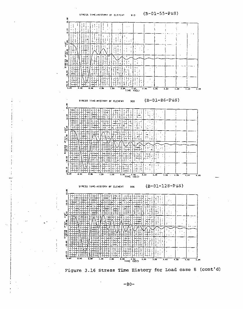
,
.,
-
,,,:
? ----
— —.-/ . .. .. . 4‘-” I -
!L—-—.-------
/“
—-—4 ..-. — ~.
-’
i.— ——. ... ....1---,>, I
J
bn 3.?0 km U.oo ..UO I
SIRESS llH[-HISIOnr Or ELEHfUI 909 (B-01-86-P&S)
:TM-.-I-.1 1-I-L-I J- U.LI 14.-I I {-++.4+ I }i4. !l. ~.!l J. :1 1 1 I 1
I ;-Li-i..l..lLlLl.l :kkki:lt!+-l+,q+lj+ :“ j-j :..j ;.. :.; II I4-I-1-i+-i.l.~-l.W1.1:-:”, In: I : I :—-— ‘---”-
1 I 1 1i,
4144-I-L14M.IX.;.4 I L;: ! 1, : ,
S~~ESS llW-H!S’TDRT OF EL[HENT 906 (B-01-128-P&S)
i
—.*“
Figure 3.16 Stress Time History
-80-
for
—. —
— .,—.. .-
,,.,—----. .- ..,_~ —
:,) . .
-—- —
. —- ----
m
8 (cent’ d)

Sln[ss 11~[.t.tlslonr of ~LFRFMT 9 ?U (B-ol-c17-P&s)
I ~ ‘
i;—. —_ ,,..
,. Ii!l“’ ,
—— ____ . .,, ]
- iI., — — . .. . .--1!!;, ;~! ., i ‘,,~! ,.. ;!,::, , ~-- .-...--—.- ;;j~i ;i:i ::I j.i.: l;; i i ‘ I,, ,, ,,::1’ -- :“ ‘—
I
“-— ..- . ,-, .
;ill. !,!, ;i,1:~ ~,$ i,,,. .!! IIw 7,.0 7.MO 3.?0 3,60 .,00’ *.”f! “1 IHE ISECI
—— .. . .—.,
STRESS 7tHL-Hlslonr or ELEMW 922 (B-01-c27-p&S)~
E.TRESS llHE-tll SlDR7 OF ELEHE)IT 921 (B-ol-c35-P&s)=
Figure 3.17
1:20 1:20
stress Time History
-81-
for Load case 9
Po
m

...
1
11
I
_..,—-,
.
I,,
-~-’—’I
I
I
1-~,------.- .:...,_..i“
-..... /j,I
..__j -. /,. .,-.—-j’--’~-.
-----! .. . 1, . . ./.
——-.. ...,,, ,,.,,,
) a.OD ,.”0
SThESS II HE-H IS1ORT ,Or ELEMENTe
91U (B-01-39-P&S)
~,,;.:;’ 1 ‘L. ---..1... .1
,,-. ,,.,,m-i ~ —---J.-.. ..- J.........;.t+:;:,:,:
w~J-1----- i i
m
D
o
Figure 3.17 Stress Time History for Load case 9 (cent’d)
-82-

5Tn(5s 71*[-Hlf7nal or EL FH[WT 913 (B-01-55-P&S)
1111”
i-H i ~—. ——_____....,.. i.
]
-{”+–+—--- I . , !
S11US5 TIHE-HISIDRY OF CLEHENT 9D9 (B-01-86-P&S)
!. I I
.—
-’----
-
,: ,,
,,,;,,;0
.. . ... J.....,.II.-......J . . . ..I
I--4---
,:— .—___
.---— - .--,
on ,.”0 ,
SlRISS TIHE-Hlsl DRT OF ELEIIEMT 906 (B-01-12 8-P &S”):
90
m
Figure
0:00
3.17 Stress Time History
-83-
for Load 9 (-cent’d)
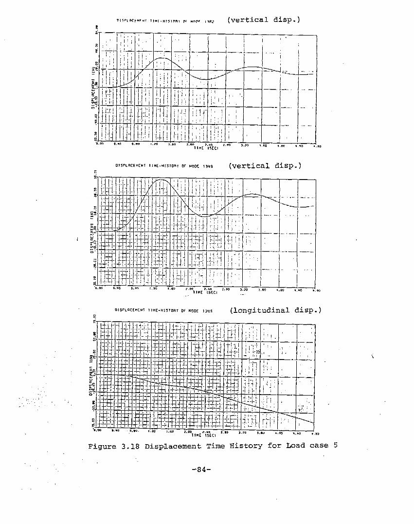
f
n15Pl Qtt WNl I) H[-H151(lR1 !lt W!IV 1 ?@.= (vertical disp.)
DIS1’LRCEMElll lIHC-HISTDRT Or MODE 13149
=
(vertical disp.)
!:1
i, ,,!1
3:”““-—....-,...._,-.:-.ff- “-L.
i’ I ..~li:
j.!+..:.”
- —. _ -.-,. -._..
4[.,~:-1,” <t, ,q : !. \ -,
:,. ‘,\..
.-. .. . .. ... —.. .— ..“, ~
;., .:!.:[, ,- “:,.
~.. :,’, — .. —.-.. . . .. . .. .-
11,,.E~;,!:. ”,. I
10 3.20 3.6D a.m 9.*O *
ml
m
D15PLRcEMEt+l I) HE- H157DR7 Of NODE 13v9
=
(longitudinal disp.)
,.-;...,,...”--- .... . . . ..’,
Figure Displacement Time History for
-84-
.—.._!.
,.
——
Load case
‘i
IO
5
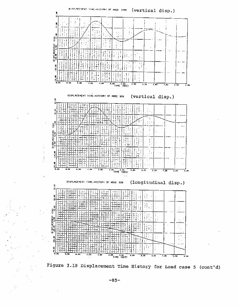
... .---
. .
-—
—..,.
.----
‘---- i_./
I
I,.-..... .._,,I. .,, _
m ● .wo
DISPLWEHEW Tl~E-HISIORT OF NODE 926 (vertical disp.)
. .llHE-i5Etl -
I
-4.—.._,.,-.—...-i
,___ .._.
‘1——.___,,_...j . .
II
;0 *.OC I
------
-..
.. . . .
. ...
,,, -..
18,HI::::;,:’‘,’: :( ,. I—--.+l-. .. ...l ..=-- I
+; :::=’ 1’’”.,,, ,,.,,%,, J-.. --1-.:. J
MO
90
Figure 3.18 Displacement Time History for Load case 5 (cent’d)
-85-

. /.:,1,
..
. . .
..
,.
,-
.
,.
...-
.“
flt5rLWFMFHl llM[. Hl$lrIRT Or wo! see (vertical disp.)
- 1“~-–+— J-.,.— ..
I
. I
1---
——
,,,-. .
..- ----
m ,.”0
o]srLrIIEHEtIT l] M[-HI$IFJRT OF NODC 339 (vertical disp.)
~
,. ... . .
. .. -_
D15rLnCEHEUl TIHE-HISIORY OF NODE JB (vertical disp.)s
Figure....;.,.3.18 Displacement Time
-86-
History for
.0
n
case 5 (cent’d)

II
‘?-.
i,.-.,I
,— ----
““l-”””....I
‘1
--
DISI’LBIEMEMI lIME-HIS70RI OF NODE J9V9(vertical disp. ):
OISPLHIEMEN1 T1HE-HI51OR7 OF NODE 1309
(longitudinal disp.)s
,,, ,,.H AH-l <4 ! . ..1....;.
1!1 : l—-–+ - ! ----
1
,:. ’.1: I:_]_ . .....I_. I
‘1
“1‘“—-’-. ._+, L
1.:..
-,!. >-” !l, ,:
-1 ..,. 1.. —-7. -– 1..–+.-..’. ..’‘.
-—.. .. .. -
‘1 ‘1-.UD ,.”~
.-
... .
Figure 3.19 Displacement Time History for Load case,.
..-’.
. ...!.. :, “’ ,’.-.~;--_f- -. .
..,..,,
-87-

Dt5F’LRCf*FMT llFI[-HISIoR? flF NODE I?3R (vertical disp.)
.’.,
,.- .:,..
.’,-. .
.. .. . . . . .
DISFlnCEHEHl llM[-M1510m OF
II1
:-.+..+=
.
-. ,-
~. . . . .
MODE 926(Vertical disp.)
-..--T-
.,.
1“=,....-.y_l .-j
-. -. .._
‘ 1-----—..- ...-...,..—..,.-,,._-.,I i
m ..00 “,” B “
D15FLRCEHEM1 lIHE-HISTORY OF NODE 926 (longitudinal disp.)s
I-- . ..L._.
I1... . _.L.
1.
“<........
,..
Figure 3.19 Displacement Time History for Load case8 (cent’d)
. -“.
-88-

!
I
-. --- .,-—
“l:-
!,
I
Ti ,
i~,“- --””””+-””“1 “ ~ ““-,,.;,/
IMl >.mSEC I
>.?0 3.s0 Uor ,,””
DISFLnCEHEWl TIH[-HIS1OFIY DF NoDE ~3g (vertical disp.)
- —— .., :.
I.,:,- —-. -.
J“~-—-.—.-...‘,,1:
, .“!!
.—. .
:;:,
-— ,.. -.. . . ..
“ /
J.........i...i...
., .,,I..-..._.,,1
. ...... -+1
I120 >.ko —m.w ..”0w t.mo
SEC) 1“ .,..
DISPLRZEMENT TIHE-MISTORr OF NODE 18 (longitudinal disp. )
1QIw_L; “““L.... .... .. !,. ].—
.,.-’- ,
:.:. ,,;,’
!.”:,:.!... ., . ..-..-, . . I--, !l. !: ’,1’, ; I—.- ----- ...-”. -.
,! 11.,.1., I.,. . ... . ,.. 19.,0. ...-
,:. .’
,,
. ...’
(cent’d)Figure Displacement Time History for Load case
-89-

Table 3.3 Peak Stress (psi)(Triangular shape,
on level–01 Deck for Load case 1Load location A)
Ship Strain Gage ElementFr. No.
Time InstantLocation
Peak StressNo. {see) (psi)
258248238228217204192150132i2810696868274635539
CF67CF60CF53CF48CF44CF39CF35CF27CF25CF17CF16CF14CF 8
B-01-128–P&s
B-01- 86-P&s
B-01- 55-P&sB-01- 39-P&s
B–ol-c44-P&s
B-01-C35-P&SB-01-C27-P&S
B-01-C17-P&S
897898899900901902903904905906907908909910911912913914915916917918919920921922’923924925
0.7600.7600.7500.7800.7600.7600.7400.7000.7400.7000.7000.6900.6900.6900.6900.6800.6800.6800.6800.6800.6800.6800.6900.6900.6901.0701.0700.6700.670
6.18.2
12.3-8.3
-32.1-45.9
5.0-127.8-202.1-423.8–467.6-532.3-560.3-554.8–492.8-511.9-597.8-610.2-532.9-506.0–439.6-333.7-182.7-225.3-195.7
–22.7-23.3117.7103.9
926 0.670 64.9927 0.670 44.1
-90-

Table 3.4 Peak Stress (psi) on level–01 Deck for Load case 2
(Concave trigonometric curve, Load location A).
Ship Strain Gage Element Time Instant Peak StressFr. NO. Location No. (see) (psi)
25824823822821720419215013212810696868274635539
Cl?67CF60CF53CF48CF44CF39CF35CF27CF25CF17CF16CF14CF 8
B-01-128-P&S
B–01– 86–P&S
B-01- 55-P&SB-01- 39-P&S
B-01-C44-P&S
B-ol-c35-P&sB-01-C27-P&S
B-01-C17-P&S
897898899900901902903904905906907908909910911912913914915916917918919920921922923924925926927
0.7400.7300.7300.7600.7500.7400.7300.7200.7400.7100.7000.7000.7000.6900.6900.6900.6800.6800.6800.6800.6800.6800.6800.6900.6900.6600.6600.6700.6700.6700.680
6.2$.6
12.9-8.3
-33.0-47.5
5.2–134.8–217.8–442.2-4e3.3–547.6-573.7-566.0-500.6-517.9-602.2-610.9-531.7-503.0-435.0-329.4-178.5-221.0-192.9
20.923.5
119.6104.964.843.7
-91-

Table 3.s Peak Stress (psi) on level-01 Deck for Load case 3(Convex trigonometric curve, Load location A)
Ship Strain Gage ElementFr. No.
Time ~nstantLocation
Peak StressNo. (see) (psi)
258248238228217204192150132128106
96868274635539
CF67CF60CF53CF48CF44CF39CF35CF27CF25CF17CF16CF14CF 8
E-01-128-P&s
B–01- 86-P&s
B-01- 55-PLSE-ol– 39–P&s
.
B-01-C44-P&S
B–01–C35-P&SB-01-C27-P&S
B-01-C17-P&S
897898899900901902903904905906907908909910911912913914915916917918919920921922923924925926927
0.6100.6000.6000.6100.6100.6000.6000.6000.6000.6000.6000.6100.6200.6300.6300.6400.6400.6500.6700.6800.6800.6900.6900.6900.6901.0601.1600.6100.6600.6700.670
6.58.8
13.3-9.0
-35.2-50.5
5.5-137.6-219.3-440.6-478.1-539.3-563.9-556.8-493.2-512.1-597.4-610.0-533.8-508.4-443.4-337.4-186.4-228.6-197.5-25.2-25.5116.7103.365.144.5
-92-

Table 3.6 Peak Stress (psi) on level-01 Deck for Load case 4(ABS theoretical bow force, Load location A)
Ship Strain Gage Element Time Instant Peak StressFr. No. Location No. (see) (psi)
25824823822821720419215013212810696868274635539
CF67CF60CF53CF48CF44CF39CF35CF27CF25CF17CF16CF14CF 8
B-01-128-PLS
B-01- 86-P&S
B-01- 55-P&SB-01- 39-P&S
B–01-C44-P&S
B-01-C35-P&SB–01-C27-P&S
B-01-C17-P&S
897898899900901902903904905906907908909910911912913914915916917918919920921922923924925926927
1.2601.2601.2601.2501.2501.2501.2600.7201.1300.7200.7200.7200.7200.7300.7300.7300.7300.7300.7400.740 “’”’0.7400.7501.0301.0301.0301.0101.0101.0101.0101.0101.020
9.010.316.0
-19.3-57.0-73.8
6.0–131.4237.7
-429.7-471.5-535.0-561.6-555.6-493.1-512.7-598.3-610.5-533.5-506.9–440.4
-334.3232.1275.7249.3-252.9-281.8-315.2-228.3-71.0-47.1
-93-

Table 3.7 Peak Stress (psi) on level-01 Deck for Load case 5
(~ 39, Load loaction A)
Ship Strain Gage ElementFr. No.
Time Instant Peak StressLocation No. (see) (psi)
25824823822821720419215013212810696868274635539
CF67CF60CF53CF48CF44CF39CF35CF27CF25CF17CF16CF14CF 8
B-01-128-P&s
E-ol- 86–P&s
B-01- 55-P&sB–01- 39-P&s
B-01-C44-P&S
B-01-C35–P&S
B–01-C27-P&SB-01-C17-P&S
897898899900901902903904905906907908909910911912913914915916917918919920921922923924925926927
0.9280.9120.9121.2160.9280.9280.9120.8960.9120.8960.8960.8960.8960.8960.8960.8800.8800.8800.8800.8800.8800.8800.8800.8800.8800.7360.7360.8640.8640.8640.864
87.2120.9182.0
–123.3-465.0-671.974.6
-1921.0-3076.0-6173.0-6628.0-7410.0-7689.0-7523.0-6567.0-6744.0-7793.0-7846.0-6814.0-6426.0-5539.0-4195.0-2275.0-2825.0-2463.0249.4282.01503.01323.0826.0561.3
-94-

Table 3.8 Peak Stress (psi) on level–01 Deck for Load case 6
(Ram 39, Load location B)
Ship Strain Gage Elament Time InstantFr. No. Location
Peak StressNo. (s.ec) (psi)
25824823822821720419215013212810696868274635539
CF67CF60CF53CF48CF44CF39CF35CF27CF25CF17
.-CF16CF14CF 8
B-01-128-P&s
B-01- 86-PLS
B-01- 55-P&sB-01- 39-P&s
B–01-C44-P&S
B–01-C35-P&SB–01-C27-P&S
B-01-c17-P&s
897898
~ 899900901902903904905906 ,907908909910911912913914915916917918919920921922923924
0.9120.9120.9120.9280.9120.9120.9120.8960.8960.8960.8960.8960.8960.8960.8960.8800.8800.8960.8960.9120.8640.8640.8640.8640.8640.8640.8640.864
925 0.864926 0.880927 0.944
63.586.6
130.9-91.0
-349.9-502.8
55.2-1388.0-2332.0-4317.0-4476.0-4871.0-4936.0-4637.0-3820.0-3575.0-3508.0-2513.0-1585.0–463.41047.01489.01661’.01426.0986.0672.5504.0344.5181.465.537.0
-95-

Table 3.9 Peak Stress (psi) on level–01 Deck for Load case 7
(%TI 39, Moving load)
Ship Strain Gage Element Time InstantFr. No. Location
Peak StressNo. (see) (psi)
25824823822821720419215013212810696868274635539
CF67CF60CF53CF48CF44CF39CF35CF27CF25CF17CF16CF14CF 8
B-01-128-P&s
B-01- 86-P&s
B-01- 55-P&sB-01- 39-P&s
B-01-c44-P&s
B-01-C35-P&SB-01-c27-P&s
B-01-C17-P&S
897898899900901902903904905906907908909910911912913914915916917918919920921922923924925926
0.9300.9200.9201.2100.9400.9300.9200.9000.9000.9000.9000.8900.8900.8900.8800.8700.8600.8500.8500.8400.8400.8400.8700.8700.8700.8700.8700.8300.8300.830
78.3107.0161.4
-109.6-423.8–608.966.7
-1721.0-2800.0-5500.0-5820.0-6437.0-6617.0-6365.0-5452.0-5440.0-5993.0-5577.0-4592.0-3757.0-2441.0-1140.01082.01166.0752.81442.01354.01091.0652.1257.5
927 0.840 137.5
-96-

Table 3.10 Peak Stress (psi) on level-01 Deck for Load case 8
(Ram 14, Load location D)
Ship Strain Gage Element Time Instant Peak StressFr. No. Location No. (see) (psi)
25a24823a22821720419215013212810696868274635539
CF67CF60CF53CF48CF44CF39CF35CF27CF25CF17CF16CF14CF 8
B-01-128-P&S
B-ol- 86-P&s
B-01- 55-P&SB-01- 39-PLS
B-01-C44–P&S
B-01-C35-P&SB-01-C27-P&S
B-01-C17-P&S
897898899900901902903904905906907908909910911912913914915916917918919920921922923924925926927
0.6720.6560.6560.6720.6720.6560.6560.6400.6400.6400.6400.6400.6400.6400.6400.6400.6240.6240.6240.6240.6240.6240.7040.7040.7040.6080.6080.6080.6240.6240.624
47.565.499.1
-67.8-262.6-378.3
41.8-1066.0-1696.0–3451.0-3752.0-4232.0-4422 ~0-4332.0-3791.0-3882.0-4420.0-4306.0-3657.0-3238.0-2477.0-1582.0-307.1-3s9.0-401.0826.1839.6941.1634.1288.7169.4
-97-

Table 3.11 Peak Stress (psi) on level-01 Deck for Load case 9(Ram 14, Load location C)
Ship Strain Gage Element T~me Instant Peak StressFr. No. Location No, (see) (psi)
25824823822821720419215013212810696868274635539
CF67CF60CF53CF48CF44CF39CF35CF27CF25CF17CF16CF14CF 8
B-01-128-P&S
B-ol- 86-P&s
B–01- 55-P&SB-01- 39-P&S
B-01-C44-P&S
B-01-C35-P&S
B-01-C27-P&S
B-01-C17-P&S
897898899900901902903904905906907908909910911912913914915916917918919920921922923924925926927
0.6560.6560.6560.6720.6560.6560.6560.6400.6400.6400.6400.6400.6400.6400.6400.6400.6400.6240.6240.6400.6401.1520.6080.6080.608 .0.6080.6080.6240.6240.6240.640
42.057.487.2
-61.6-235.1-338.1
37.2-944.8
-1534.0-3022.0-3238.0-3615.0-3746.0-3615.0-3102.0-3085.0-3329.0-2926.0-2282.0-1600.0-608.7-177.51062.01091.0754.3795.2695.7497.5268.394.744.0
-98-

. . .... .
Table 3.!2 Summary of Results for Load Cases
1 i I I I I 1 I I r
I LC 1 I Lc 21.( LC3~ LC 4 I LC5~ LC 6 ~ LC7~ I.-C 8 I LC9j
Shape of Ice Load i, Triangular
/
Peak Bow Force (MN)I
2.0
Duration T (see)
Time to reach
Peak force (see)
IBow Force Location
u) (Frame No.)
w
I
Calculated
Peak Stress (PsI)
Location of
Peak Stress
Time Instant of
Peak Stress (see)
fJeasured
Peak Stress (psi)
1.0
0.667
ACF2t-25
610.2
8-01-39
-P&s
O. 680
, ,
ConcaveI
ConvexI flBs
curve curve/
I
2.0/ 2-0 ! 2“0
1.0/
1.0 I 1.0
IO. 667 I /
0.667 , 0.728
A iAiACF21-25 i
ICF21-25
/CF21-25
II
I
610.9 I II
610.0 610.5
/
0-01-39 i II
B-Ot-39 B-01-39-P&s
I-Pi?s -P&s
/
0.680 I II
O.650 0.730
/
1-1-
f 1 1 L I
Ram 39 /Ram 39 i
I?am 39i Ram 14 /
1 IRam 14 i
I I II I I
25. I 25. i 25 i / iI “ I ‘6”
$6.
1.1 I1 ‘“’ I ‘“i I
0.85 Ii 0.05
I / i II
/0.65 I
/0.65
I0.65 0.50 , 0.50
I
A I ~ i *TOC i I iCF21-25 1 0 I ~F3:.37 I
!CF41 -45 CF21 -25
1 To ICF25-29
1
1 I1
CF33-37/ !I
I I t I7846. II 4936.
I66t7.
I4422.
13746.
I
1 I II
iI
i8-01-39 0-0! -86 6-01-86 J
/B-01-86
I8-01-86
-Pas/
-P&s -P&s -P&s -P&s //
tI
II
0.080 I I i/ O. 896 0.890 0,640 0.640 i
1 I/ / I /
6078.I
6078. ! 6078. / /1
2554. 2554.t
J I t I I

the forward end of the ship. Typical stress time histories for element 914 fromload cases 2 and 3 show that during the 1 second period of application of theimpact loads, the response follows closely the shape of the forcing functions.After the initial 1 second, the vibration response damps out quite rapidly asthe impact ends. The peak stress value for element 914 was found to be 611 psiat a time instant of 0.68 second in load case 2 and 610 psi at a time instant of0.65 second in load case 3.
These results indicated that the peak stress values obtained for the threeload cases were about the same in magnitude, although the time instant at whichthe peak stress occured did vary slightly.
In the present analysis, a fourth load case was carried out using ABS theore-tical bow force time history curve (Figure 3.4). The stress response curves arepresent~ in Figure 3.12. The response for strain gage B-01–128-P&S again showstwo-node bending vibration after the impact load ends. For other locations be-tween ship frame 128 and cant frame CF44, the response follows the pattern ofthe applied bow force time history and reaches the peak stress at abut 0.,73second, which was the time to the peak of the bow force time history curve. Itis noted that the response exhibits a sharp reversal of stresses immediatelyfollowed the 1 sec duration of the impact force. This pheonmenon is attributedto the unloading rate of the impact force. Referring to the ABS theoretical bowforce curve, it is observed that the slope of the unloading branch is quitesteep compar= to the loading branch. The maximum peak stress obtaind in thiscase is 610 psi at location B–01-39-P&S.
It is interestd to note that the peak stresses obtained in load case 4 areabout the same as those in load cases 1 to 3. In all four cases, the impactforces were applied at the same location A and the bow force histories had thesame peak value of 2 MN and the same duration of 1 second. The difference be-tween load case 4 and load cases 1 to 3 was that the time to peak force for loadcases 1 to 3 was 0.667 second and for load case 4 was 0.728 second. The loadingbranches were abut the same. In fact, it was noted that the loading ”branchforload case 4 fell between the loading branches of load cases 1 to 3, althoughload case 4 had a longer time to reach the peak force. In contrast, the unload-ing branch of load case 4 fell outside the bound of load case 3 and was muchsteeper. As a result, a sharp reversal of stresses occurr~ in load case 4.Based on the calculated results, it was found that the stress time histories ob-tained for these cases were quite similar following the pattern of the loadinghistories.
This initial phase of Study shows that the dynamic response of the hullgirder is predominantly correspond~ to the two-node banding rncde and the re-sponse followed closely to the shape of the forcing functions. This also setvdas a bench mark check in using the finite element mtiel in the subsequent study.
The next three cases (load cases 5 to 7 ) utilized the actual tiw force timehistory of Ram 39. Emphasis was given to the locations where the vertical lmwforces were applid.
Figure 3.13 shows the stress time history results for load case 5 in whichthe bw force was applied to location A between cant frames 21 and 25. As ax”
-1oo-

petted from the initial study, the dominant vibration was found to be thetwo-ride bending mode having a vibration frequency of shut 3.1 Hz. The maximumpeak stress value was determin~ to be 7846 psi occured at a time instant of0.88 second. This was located at element 914 corresponding to ship frame 39.
Similarly, by examining the element stress time history for load case 6 inwhich the lmw force was applied to location B between cant fm.mes 41 and 45,thesame phenomenon as in load case 5.was obtaind. However, the location at whichthe maximum peak stress occured shifts towards the aft of the ship to element909 (B-01-86-P&S) instead of 914 (B-01-39-P&S). The maximum peak stress was4936 psi, as compard to 7846 psi in load case 5, and occur~ at a time instantof 0.896 second. For this case, the peak stress obtaind for element 914 was2513 psi at a time instant of 0.896 second. These results indicated that bychanging the location of the applid hw forces from location A to location B,the maximum peak stresses dropp~ from 7846 psi to 4936 psi,occuring at differ-ent sections of the hull (see Tables 3.7 and 3.S).
For simplicity, the above two load cases assumed that the location of the bowforces was stationary during the entire duration of load application. To simu-late more closely the case in reality, it became necessary to use moving loadswith the actual measured time history of Ram 39. The impact velocity of 4.4m/see given in the ARCTEC report was assumed to be constant during the impactand the vessel moved with that velocity for a duration of 1.2 seconds. The datapreparation for this case was much involvd since the forcing function changedwith time along the center line stem bar. In this particular case, the numberof time functions had to be limitd to 30 becasue of the limitation of SAP-Vcomputer program. The results of this load case 7 are presented in Table 3.9and in Figure 3.14. The maximum peak stress was found to be 6617 psi at a timeinstant of 0.89 second. This occurred at element 909 corresponding to straingage location B-01-86–P&S”.
By comparing the results of these seven load cases, it is riot~ that thevariation of the peak stress values is not significant for different shapes ofthe forcing functions, if the loads are applied to the same location. The peakstress values obtain@ are about the same and the location at which the maximumpeak stress occurr~ is also the same. For example, the maximum peak stressesfound in load cases 1 to 3 were about 610 psi at location B-01-39-P&S for theapplied vertical bow force of 2 MN. Because of the linear elastic analysis,this peak stress would be 7625 psi if the Ram 39 vertical force of 25 MN is ap–plied to the same location A. In comparison, the maximum peak stress obtainedin load”case 5 when using Ram 39 lmw force was 7846 psi, a ratio of 1.03. Thisvariation could be attributd. to the difference in shapes of the forcing func–tions.
Although the variation of peak stresses was insignificant when impacts wereappli~ to the same location, it became considerably more significant when im-pacts were applid to different locations. For the two extreme locations~ des-ignated as location A and location B, for Ram 39 presented in load cases 5 and6, the upper and lower lxunds values of the peak stresses were obtained. Forload case 7 where the ~ 39 loading was allow~ to move at constant velocitybetween location A and B, the peak stresses were found to be within the twobunds. The maximum peak stress for load case 7 was locat~ at B-01-86-P&S hav-
-1o1-

ing a value of 6617 psi at the time instant of 0.89 second. From the measurddata of Ram 39, the maximum peak stress was found to be 6078 psi. In this case,the ratio of the maximum peak stress between the finite element analysis to themeasured data is 1.09.
The next two load cases use Ram 14 hw force history appliad to locations Dand C, respectively. Basal on the measured data of Ram 14, the load locationfor the measured time of 13.0 and 14.0 seconds was nearly stationary in way ofcant frame 27. This corresponded to load case 8 where the load was applied tolocation D. The calculatd maximum peak stresses were found to be 4422 psi and3746 psi, respectively, for load cases 8 and 9, both occuring at the same straingage location of B-01-86-P&S and at the same time instant of 0.64 second.Again, this analysis indicated that load case 8 showed higher peak stress thanload case 9 in which the load location C was more towards the aft of the vessel.The measured maximum peak stress obtained from the Ram 14 was 2554 psi, whichwas lower than both load cases 8 and 9. The ratio? of the maximum peak stresscompared to load cases 8 and 9 were 1.73 and 1.47, respectively. Using Ram 14loading, the corriparisionwas not as good as that using Ram 39 loading. This
- study showed that in addition to the peak magnitude and time history of the im-pact load, the exact location at which impact takes place and the impact veloc-ity are important in order to obtain a correct dynamic response.
-lo2–
4. CONCLUSIONS
1. The test data acquired during the POLARa substantial contribution to thedeveloping a practical analytical model
SEA deployment in 1985 isdatabase available forof ship/ice impact. The
test data analysis shows that the analytical model used is capableto predict the impact loads due to ramming icebreaking. The modeldescribes well the total force history and gives reasonableestimate of the force magnitudes. For more accurate forceprediction the model should be further refined. However, twofactors make it impossible to adjust the mathematical modelthe presented test data.
A. Insufficient Ice DataSince the impact load parameters (forces, pressure, timehistories, etc.) depend on many variables {such asmasses, shapes, velocities, etc. ) it is essential tomeasure all of the variables or maintain theunmeasurable variables constant during the tests. It isvery difficult, if not impossible, to fulfill thiscondition when ramming ice ridges. The presented datadoes not contain sufficient information on the variablesrelated to ice, such as the shapes and masses of the iceridges, its homogeneity, dynamic crushing strength ofice, etc, Since some of the ice parameters in equations(1)-(7) could vary randomly during the tests and theirvalues and changes are unknown, one can hardly expectaccurate results for each particular events, even if theequations are perfect. Therefore, the inaccuracy of thecalculated ice forces, which takes place for some peakforces such as 3-(l), 3-(2), 17-(3), 25-(3), 26-(1) inTable 5, should rather be related to the insufficientice data.
B. Insufficient velocity dataThe velocity data contains only the horizontal velocityrecords which often are interrupted. A majority of therams have resulted in successful breaking through theridges. Many of the rams, consisted of consecutiveimpacts followed by beachings. In such conditions thehorizontal velocity history, even if accurate, does notcharacterize the penetration (crushing) velocityhistory. The latter can be obtained if an additionalvelocity or acceleration component is measured, such asvertical velocity of the bow, or pitching accelerationsor others.
2. The analytical model described in Section 2 can predict the
using
loadsdue to ship/ice impacts, both in general, and ‘specifically forramming icebreaking. Even at its present form given by equations(3)-(7) it gives reasonable estimates of ramming forces. Further
- 103 -

developments of the model are desirable and feasible, bothanalytically and experimentally.
3. The analytical efforts should be concentrated on widening themodel’s applicability. Ice impacts against ship sides andappendages should be specified in detail for various shapes ofship structures and ice features. Post-impact beaching forcesshould also be included in the model.
4. The experimental studies, which can be most valuable for theanalytical model and less expensive, may include:
- Ramming tests on very thick level ice, eithergrounded or floating. If such a field is found, itsmass, shape, strength and’ homogeneity can bespecified accurately enough to assme it virtuallyconstant during the trial. As a result, onlyseveral rams would give sufficient, reliable andinterpretable information on ice loads both duringthe impact and beaching phases. Those tests canestablish experimental dependence of the rammingloads on the ramming speed - which is the principalvariable in any model.
- Ramming tests at various size bergy-bits of glacialice. The main variables in such tests can be theice mass (and consequently the reduced ship/icemass) . Since ice properties of freely floatingglacial ice can be assumed virtually constant, whileice shapes vary randomly, the number of rams shouldbe sufficient for statistical confidence.
- In-situ ball.dropping or pendulum tests. In thesetests all variables can be accurately recorded andcontrolled. As a result, the tests can provideinformation on the effects of many variables, aswell as the values of the dynamic crushing strengthof ice.
5. Based on the dynamic analysis of the finite element model, thedominant vibration was the two-node bending mode of the hullgirder, having a natural frequency of 3.1 Hz. The frequencyagrees very well between the calculated and measured results.
6. The dynamic response showed ihat the shape of the stress timehistory curve followed closely to the shape of the applied bowforce tune. In this study, the maximum peak stresses obtained inload cases 1 to 4 were about the same for the same peak value ofthe unit impact load and impact location, although the shape ofthe applied bow forcd was different. Therefore, the maximum peakstress value was not significant to the shape of the bow force,This may be due to the fact that the resonance did not occur inthis case.
- 104 -
7. It was found that the exact location at which the impact bw forceoccurred was an important factor in the peak stress values. The maxi-mum peak stress obtained was higher when the bow force was appliedmore towards the forward end. It is noted that efforts are made to-wards the prediction of the magnitude and shape of the ice force bothby analytical means and by measurements. It is equally important toinclude the effort in determining the exact location and distributionof the ice force where the impact occurs in order to more accuratelypredict the structural response. The velocity of impact and the move–merit of the ice force along the center line keel also contributes tothe acccurary in obtaining the dynamic response of the analyticalmodel.
8. The maximum peak stresses obtained from the finite element analysisand the measured value did not agree quite well in the case when usingRam 14 loading, whereas in the case of Ram 39 moving load, the maximumpeak stresses agree very closely. The difference in results attri-buted partly to the inaccuracy in defining the location of the iceramming load and its movement in the measurements and partly to thein’herentdifferences in the two methods in obtaining the stresses. Inthe finite element analysis, the response represents the coupledinteraction of the entire hull structure of the three dimensional fi–nite element model. On the other hand, the beam idealization of thehull girder used in the measurements is of two dimensional and the ef–feet of shear deformation is neglected. In this regard, the’ assump-tion of beam behaviour in relating the measured stress to the bendingmomerrtmay contribute to inaccuracy in obtaining the magnitude of kwforce.
.,-.
–lo5-

5.
1.
2.
3.
4.
5.
6.
7.
8.
9.
REFERENCES
Brown, T.G., Kocaman, A., Punj, V., Bertha, F,G. Iceberg-Structure Interaction Global and Local Loads, Proc. OMAE-86,April 1986, Tokio, Japan, Vol. 4, pp 374-378.
Glen, I.F., Comfort, G. Ice Impact Pressure and Load:Investigation by Laboratory Experiments and Ship Trials. Proc.POAC-83, Helsinki, Finland, April 1985, Vol. 1, pp 516-533.
Kheisin, D.E., Likhomanov, V.A., Kurdyumov, V.A. Determination ofSpecific Crushing Energy and Contact Pressures due to Solid/IceImpact. Trans. Arctic & Antartica Research Institute, Leningrad,1975> Vol. 326, pp 210-218, (in Russian). English drafttranslation by CRREL, TL539, 1976.
Kurdyumov, V.A., Kheism, D.E. A Hydrodywoic Model of Solid/IceImpact. Applied Mechanics, Kiev, 1976, Vol. XII, #10, pp 103-109.
Kurdyumov, V.A., Kheisin, D.E. Determination of Ice Loads Actingupon Icebreaker Hull Due to an Impact. Trans. LeningradShipbuilding Institute, issue 90, 1974, pp 95-100 (in Russian).
Nevel, D.E. Iceberg Impact Forces. Proc IAHR Ice Symposium-86,Iowa City, Iowa, August 1986, Vol. 3.
Tunik, A.L. Dynamic Ice Loads on a Ship. Proc IAHR Ice Symposium1984, Hamburg, F.R. Germany, August 25-31, 1984, Vol. 3, pp 227-313.
Tunik, A.L. Hull Girder Bending Forces due to RammingIcebreaking. Proc POAC-85, Narsarssuag, Greenland, September1985, Vol. 2, pp 873-881.
Bathe, K.J. and Wilson, E.L. “Stability and Accuracy Analysis ofDirect Integra~ion Methods”, International Journal of EarthquakeEngineering and Structural Dynamics, Vol. 1, No. 2, 1973,
- 106 -

--.>

APPENDIX A
Finite Element Model

Figure A-1 01-Level Deck
Figure A-2 Main Deck

o

\
al
A-3
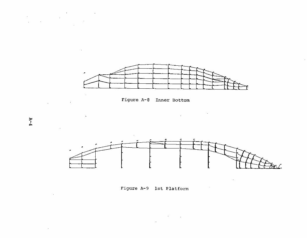
.- — — ._
Figure A-8 Inner Bottom
.
. ,- .,..1-
~ I
<
=EE
Figure A-9 1st Platform

...“
A
A-5

,“
—
—.-
——
ZLil-in
Figure A-12 Center line Vertical Keel

. :,,,,.. , . . . .... .
Figure A-13 Shafting, 15 ft.- 21 ft. off C.L.
.
h . . . -— - .
. . . . . . -
Figure A-14 Long. Bhd, 26 ft. 6 in. off C.L.
.
Figure A-15 Long. Bhdr 4 ft.- 14 ft. off C.L.

Figure A-16 Pilot House

C4
●
+,
●
$4
lo
A-9

-+ E●
: .
❑ ■
m
●
k’P-1
a)L1
.%v-l
A-10
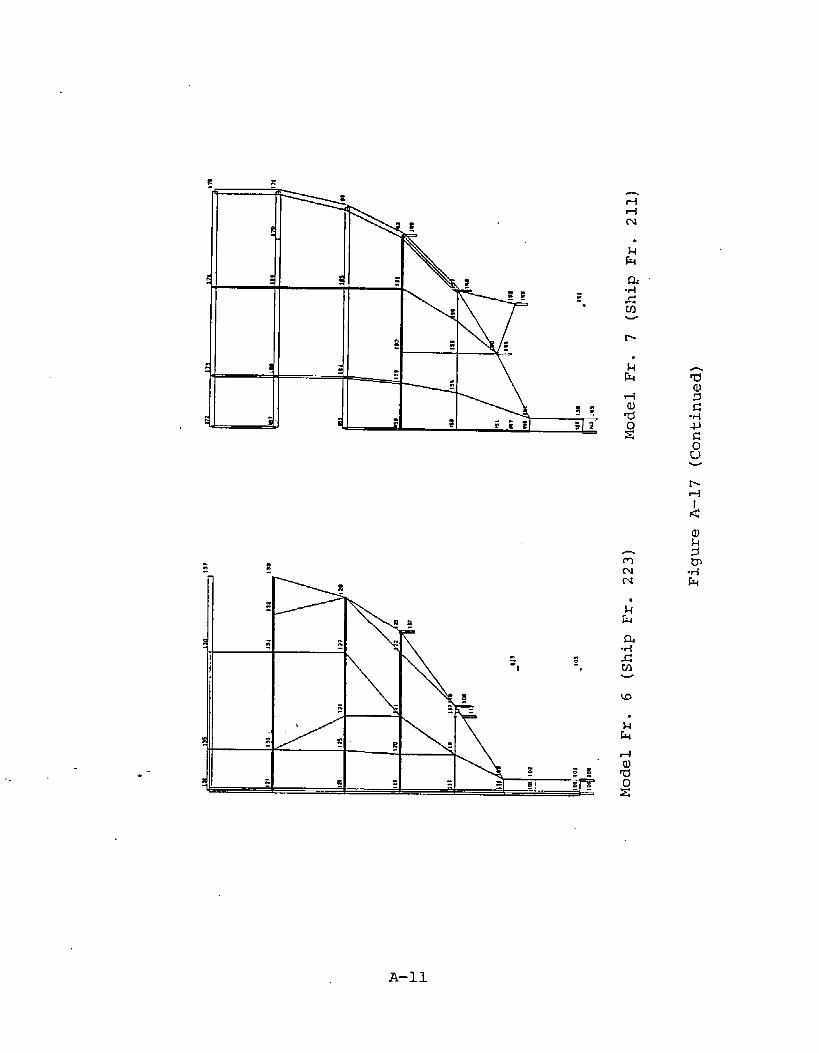
.. ● ✍
=+
r-
—
m‘a
N
1+
-PiJJ
A-n

m
m
-51-l
r-L+
A-12

-wu-l4
.
k’
Q4-dLccl
4
.
A-13

4
-I-l

: a
:. 8
a Ind
4
%’2
n
:d
z
El
A-15

nmm
.
k’
A-16

..
nmm
l-l
%’2
b-dsm
w
AalL1
A-17
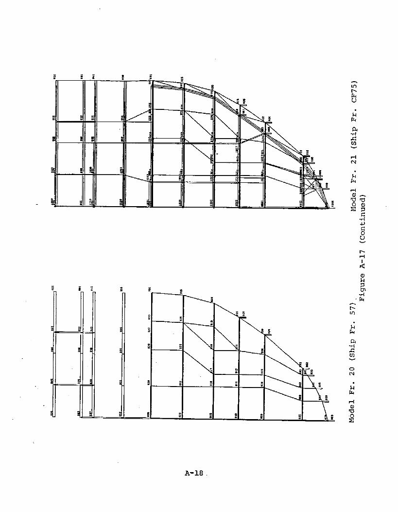
u
u
A-18

low tom1
El*1 mw
t010 $03D
M10s4 10?1
I
Model Ft. 22 (Ship Fr. CF69) Model Fr. 23 (Ship Fr. CF64)
Figure A-17 (Continued)
‘1

071 110$
Mode,l Fr. 24 (Ship Fr. CF56) Model Fr. 25 (Ship Fr. CF51)
Figure A-17 (Continued)
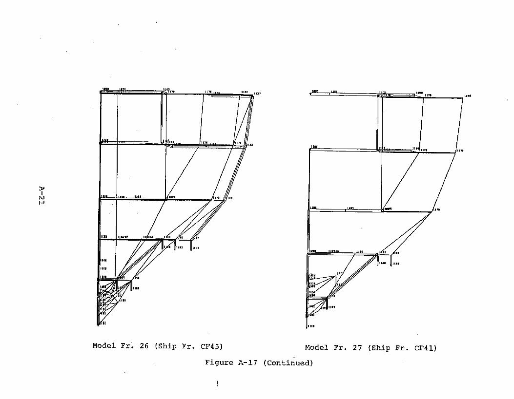
P
ML
4
1191
154
Model Frg 26 (Ship Fr. CF45)
[mlP’ , #
1m
J,,,,
Model Fr. 27 (Ship Fr. CF41)
Figure A-17 (Conti~ued)
I

“i.,
n
Fmbv
A-22
w
A

.
-., *“
.
w
om
A-23

A-24

m0-l
n
., .
A-25