numerical simulations of the ice load of a ship navigating...

Computer Modeling in Engineering & Sciences CMES, vol.121, no.2, pp.523-550, 2019

CMES. doi: 10.32604/cmes.2019.06951 www.techscience.com/cmes

Numerical Simulations of the Ice Load of a Ship Navigating in Level Ice Using Peridynamics

Yanzhuo Xue1, Renwei Liu1, Yang Liu1, *, Lingdong Zeng1 and Duanfeng Han1

Abstract: In this study, a numerical method was developed based on peridynamics to determine the ice loads for a ship navigating in level ice. Convergence analysis of three-dimensional ice specimen with tensile and compression loading are carried out first. The effects of ice thickness, sailing speed, and ice properties on the mean ice loads were also investigated. It is observed that the ice fragments resulting from the icebreaking process will interact with one another as well as with the water and ship hull. The ice fragments may rotate, collide, or slide along the ship hull, and these ice fragments will eventually drift away from the ship. The key characteristics of the icebreaking process can be obtained using the peridynamic model such as the dynamic generation of cracks in the ice sheet, propagation and accumulation of ice fragments, as well as collision, rotation, and sliding of the ice fragments along the ship hull. The simulation results obtained for the ice loads and icebreaking process were validated against those determined from the Lindqvist empirical formula and there is good agreement between the results. Keywords: Peridynamics, ice load, level ice, ship-ice interaction, ice properties, convergence.

1 Introduction As the demand for oil continues to increase over the years, oil companies are constantly searching for new oil reserves. It is estimated that 25% of the world’s hydrocarbons are located in the Arctic. However, oil and gas exploration in the Arctic poses a significant challenge due to the extremely low temperatures and ice conditions in this region. With global warming on the rise, the thinning of ice sheets in the Arctic shortens the season in which activities can be carried out. However, the melting of sea ice driven by global warming will make it possible for commercial non-ice-strengthened ships to navigate along the edges of the Arctic, which will significantly reduce the distance between trading ports and thus, shipping times [Kwok and Cunningham (2012)]. Ship navigation in level ice leads to continuous breakup of the ice sheet into fragments. These ice fragments occupy a certain space within proximity of the ship, resulting in periodic and impulsive ice loads. The maximum ice load typically occurs within a relatively short period and most of the time, the ice load remains at a low level. Hence, it is crucial to fulfill the design requirements of ice-strengthened vessels such as bow structural strength, fatigue strength, ice-induced vibrations, and ice resistance. Numerous

1 College of Shipbuilding Engineering, Harbin Engineering University, Harbin, 150001, China. * Corresponding Author: Yang Liu. Email: [email protected].

524 CMES, vol.121, no.2, pp.523-550, 2019

models have been developed to model ice-induced loads on the shell structure of ships. However, it is particularly challenging to develop reliable models that can accurately simulate the prevailing loads acting on the ship hull. Various methods have also been developed to predict the ice resistance of ship hulls. The reader may refer to previous studies [Daley (1991); Enkvist (1972); Kheisin and Popov (1973); Kujala (1994); Kujala and Vuorio (1986); Kwok and Cunningham (2012); Leira, Børsheim and Amdahl (2009); Varsta (1983); Vuorio, Riska and Varsta (1979)] for a detailed treatment on the statistical analysis of ice loads acting on ship hulls. Models have also been developed based on the finite element method (FEM) to predict ship-ice interactions and ice loads [Han, Feng and Yue (2007); Kolari, Kuutti and Kurkela (2009); Nylandsted, Jäättelä, Hoffmann et al. (2003); Premachandran and Horii (1994); Ranta, Polojärvi and Tuhkuri (2018); Xue (2016)]. The discrete element method (DEM) has been used to model various ice-related applications including real-time simulations of ship-ice interactions [Lubbad and Løset (2011)], modeling the ship behavior in broken ice [Karulin and Karulina (2011)], dynamic positioning in ice [Metrikin, Løset, Jenssen et al. (2013)], and ice floes jamming in rivers [Stockstill, Daly and Hopkins (2009)] as well as modeling ice ridges and ice rubble in conjunction with FEM [Arttu and Jukka (2009); Paavilainen and Tuhkuri (2013)]. Metrikin et al. [Metrikin and Løset (2013)] provided an excellent review of different types of DEMs and the applications of DEMs in solving ice-related problems. However, due to differences in the discretization schemes between FEM and DEM, guaranteeing continuity at the solid boundaries using FEM-DEM coupled methods is not possible. Some of the disadvantages of using FEM in modeling the progressive failure of ice include mesh tangling and the use of erosion models to predict the failure patterns of ice [Das (2017)]. According to Di et al. [Di, Xue, Bai et al. (2017)] even though DEM is capable of capturing the discontinuous phase of the fracturing process, the method is less accurate when it comes to modeling the whole fracturing process from the continuous to discontinuous phase. Deb et al. [Deb and Pramanik (2013)] highlighted that when DEM is used, it is essential to conduct extensive calibration to identify the parameters for deformability and strength. Still model tests are the best method to measure the ice resistance of new ship hull designs, which have significantly improved over the last few years. Zhang et al. [Zhang, Shang and Zhang (2013)] conducted still model tests to determine the minimum engine power output for an oil tanker built for ice class 1A. The ice loads of an icebreaking vessel navigating in the Baltic Sea predicted by empirical formula and computational fluid dynamics were compared with those obtained from still model tests [Kim, Kim, Sim et al. (2015)]. A medium-scale still model test system was also built by Konno et al. [Konno, Nakane and Kanamori (2013)] to study ice-structure interactions, where the system was used to examine the different modes of dynamic ice loads and structural responses of narrow compliant structures such as the drilling platforms in Bohai Bay. Huang et al. [Huang, Ma and Tian (2013)] observed the ice failure modes and structural responses for different ice conditions and structural stiffnesses. Zhang et al. [Zhang, Wang, Gu et al. (2012)] established a speed measurement and positioning system for moving air cushion loads and they measured the mechanical properties of ice-like materials and the pressure distributions of air cushion loads. Luo et al. [Luo, Guo, Wu et al. (2018)] conducted ice resistance tests of a ship model under the combined effects of waves and ice floes and the results showed that the motion of the ship model was more unstable in the marginal ice zone than in ice

Numerical Simulations of the Ice Load of a Ship Navigating 525

floes. Even though still model tests in ice tanks are typically used to investigate the ice loads of ships navigating in Arctic areas, these tests are time-consuming and costly, especially in the design and optimization of hull forms [Kim, Lee, Lee et al. (2013)]. Meshfree methods are certainly advantageous to model the fracturing process and crack growth of ice sheets because these methods are independent of the element grids during the computational process [Han, Zhang, Wang et al. (2018); Li and Liu (2002); Wang, Wang, Zan et al. (2017)]. Libersky et al. [Libersky and Petschek (1991)] first applied the Smoothed Particle Hydrodynamics (SPH) approach to solid mechanics. Benz et al. [Benz and Asphaug (1994)] extended their work to simulate the fracturing process in brittle solids. Zhang et al. [Zhang, Zheng and Ma (2017)] embedded the Drucker-Prager model into the SPH code in order to simulate the four-point bending and uniaxial compression failure of ice. The cohesion softening elastic-plastic model has also been used within the SPH framework. Even though SPH is advantageous to numerically solve large deformation problems, its convergence has not been proven theoretically and therefore, there is a need to improve the accuracy of the solution [Li and Liu (2002)]. In order to overcome this limitation, Silling in 1998 coined peridynamics, which is reformulation of the classical continuum mechanics. In this approach, a force density function (also known as the pairwise force function) is used for each pair of particles and it is postulated that the particles interact with one another across a finite distance [Silling (2000); Silling and Askari (2005)]. Unlike molecular dynamics, peridynamic modeling has constitutive properties that are dependent on the reference configuration. In addition, unlike continuum mechanics, peridynamic modeling does not require a continuous response field [Gerstle (2015)]. Peridynamics is superior to solve discontinuous problems such as fracture in quasi-brittle solids [Ren, Zhuang, Cai et al. (2016); Fan and Li (2017); Gu, Zhang, Huang et al. (2016); Lai, Liu, Li et al. (2017); Ni, Zhu, Zhao et al. (2017); Ren, Zhuang, Rabczuk (2017); Rabczuk and Ren (2017); Wang, Zhou, Wang et al. (2018)], and in composite Structures [Cheng, Zhang, Wang et al. (2015)]. A couple of studies have been carried out to simulate the ice loads and ice-structure interactions using peridynamics [Liu, Wang and Lu (2016) ; Ye, Wang, Chang et al. (2017); Wang, Wang, Zan et al. (2017); Liu, Xue, Lu et al. (2018)]. Even though there are a few studies concerning the use of peridynamics to simulate ice loads and ice-structure interactions, none of these studies are focused on the investigating the key characteristics of ship-ice interactions in continuous icebreaking mode, which forms the objective of this study. The effects of ice thickness, sailing speed, and ice properties on the mean ice loads during the continuous icebreaking process were also investigated. This paper is organized as follows. The kinematics of bond-based peridynamics is described briefly is in Section 2. Convergence analysis of three-dimensional ice specimen with tensile and compression loading and the determination of the micro-parameters of ice are presented in Section 3 while the simplifying assumptions (specifically the gravitational and buoyancy forces) and development of the ship-ice interaction model are presented in Section 4. The results obtained from the peridynamic model were compared with those determined from the Lindqvist empirical formula, which will be presented and discussed in Section 5. The effects of ice thickness, sailing speed, and ice properties on the mean ice loads are also presented in this section. Finally, the conclusions drawn based on the findings of this study are presented in Section 6.

526 CMES, vol.121, no.2, pp.523-550, 2019

2 Kinematics of bond-based peridynamics In peridynamic modeling, the internal force acting at a particular point i in a continuum solid is defined as a function of the reference location Xj and the deformed location xj of the neighboring point j with respect to the reference location Xi and the deformed location xi of point i. The peridynamic equation of motion for point x in the reference configuration at time t is given by:

( ) ( , ) ( , , ) ( , )H

t t dV tρ ′′′ ′ ′= − − +∫x

xx u x f u u x x b x (1)

where V ′x is the volume of material point ′x , Hx is called the family of x, u is the displacement vector field, b is the body force density field, ρ(x) is the density field, and ′′u (x, t) is the acceleration field. The vector-valued function f is assumed to be a function

of the undeformed bond (relative position), which is given by ξ=x’-x, and the deformed bond (relative displacement) of the reference points ′x and x, which is given by η=u( ′x , t)-u(x, t). The vector ξ+η describes the relative position of the reference points x′ and x in the current configuration.

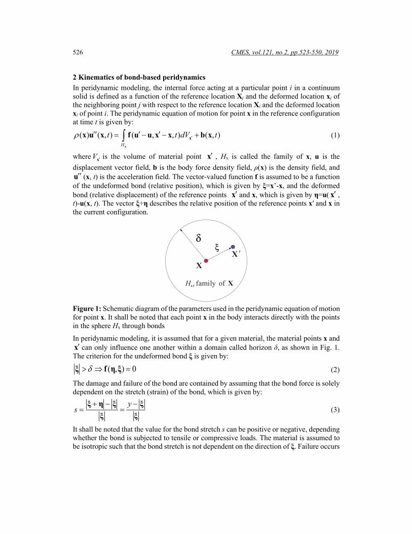
Figure 1: Schematic diagram of the parameters used in the peridynamic equation of motion for point x. It shall be noted that each point x in the body interacts directly with the points in the sphere Hx through bonds

In peridynamic modeling, it is assumed that for a given material, the material points x and ′x can only influence one another within a domain called horizon δ, as shown in Fig. 1.

The criterion for the undeformed bond ξ is given by:

( , ) 0δ> ⇒ =ξ f η ξ (2)

The damage and failure of the bond are contained by assuming that the bond force is solely dependent on the stretch (strain) of the bond, which is given by:

ys

+ − −= =

ξ η ξ ξξ ξ

(3)

It shall be noted that the value for the bond stretch s can be positive or negative, depending whether the bond is subjected to tensile or compressive loads. The material is assumed to be isotropic such that the bond stretch is not dependent on the direction of ξ. Failure occurs

XX＇

Hx, family of X


if the bond stretch is greater than its predetermined value and the bond will no longer bear any force. The bond force for a prototype micro-elastic brittle material [Silling and Askari (2005)] is defined by:

( ( ), ) ( ( , )) ( , )f y t g s t tµ=ξ ξ ξ (4) where g(s)=cs and it is a linear scalar-valued function. Here, c is the bond constant, which is also known as the micro-modulus. Without going into the detailed derivation (Equating the expressions for strain energy density obtained by classical continuum mechanics and peridynamics in terms of both isotropic expansion and simple shear, see Madenci et al. [Madenci and Oterkus (2014)], one can obtain,

4

3

2

18 , for 3D

12 , for 2D

2 , for1D

ch

A

κπδκ

π δκδ

=

(5)

where κ is bulk modulus, h equates size of particle in 2D, and A is cross-sectional area. The parameter μ(t, ξ) is a history-dependent variable, which is defined for each bond that changes suddenly and irreversibly from 1 or 0 when the bond breaks. The parameter μ(t, ξ) is defined as:

01 if ( , )( , )

0 otherwises t s

tµ′ <

=

ξξ (6)

where s0 is a constant known as the critical bond strain, which is the strain when the bond breaks. In the prototype micro-elastic brittle material model, s0 can be calibrated based on the measured critical energy release rate G0 for a brittle material [Madenci and Oterkus (2014)]. The critical bond strain is given by:

0

00

0

5 , for 3D9

, for 2D33 , for1D

G

Gs

G

κδπκδ

κδ

=

(7)

In peridynamic modeling, the crack growth is an autonomous process and it can be monitored by defining the local damage field φ(x, t), which is a fraction of the broken bonds connected to a point. The local damage field can be determined by:

528 CMES, vol.121, no.2, pp.523-550, 2019

( , , )( , ) 1 H

H

t dVt

dV

µϕ = −

∫∫

x

x

ξ

ξ

x ξx (8)

3 Parameters determination 3.1 Peridynamic parameters for ice Peridynamic body is discretized in a number of particles each describing some amount of volume and the side of a particle is commonly called a lattice. The results depend on particle positions, spacing dx, and material’s horizon δ. Horizon mainly refers to the domain of influence which defines the range of interactions between material points. It can also be considered as a length-scale parameter which gives peridynamics a “non-local” character. The size of the horizon changes depending on the nature of the problem [Bobaru, Yang, Alves et al. (2009); Freimanis and Paeglitis (2017); Han, Lubineau, Yan et al. (2016)]. For three-dimensional analysis the most common are cubic lattices with uniform spacing in all directions, and the horizon may be chosen according to convergence, since for any value of δ, the parameters in the peridynamic material model can be chosen to match the measured Young’s modulus of the material, and physical behaviour can be accurately represented.

Table 1: Critical strength (N) for compression simulation cases

δ (mm) M=δ/dx

1.015 2.015 3.015 4.015 5.015 1 33138.641 29062.049 27501.703 28713.911 28675.921 2 33137.581 28263.849 26585.102 27585.973 28172.599 3 33135.222 26968.817 25912.281 27133.463 29142.365 4 33141.656 25809.223 26499.357 26735.240 26973.669 5 33126.821 23664.238 24450.887 25731.424 26071.913

In this study, tensile and compression simulations with different horizon sizes and particle spacing combinations are performed with a constant loading velocity of 0.01 m/s, respectively. The numerical model of the specimen is established by 70×70×175 mm uniformly sized particles. According to the work conducted by Freimanis et al. [Freimanis and Paeglitis (2017)], more accurate results can be obtained using horizon sizes that are not equal to the lattice size multiplied by some integer number, so there is a suffix.015 in next investigation. The tensile and compressive strength takes the value of the maximum stress when the fracture occurs, and the results for compression and tension obtained using peridynamics are in Tab. 1 and Tab. 2, respectively. Values from experiment for compression and tension are about 27440 and 5512.5 N. Critical strength dependence on changes in M=δ/dx (the lattice size) as the horizon size stays constant is shown in Fig. 2.


Table 2: Critical strength (N) for tension simulation cases

δ (mm) M=δ/dx

1.015 2.015 3.015 4.015 5.015 1 6549.856 5776.824 5463.308 5559.381 5729.551 2 6594.540 5657.515 5329.511 5514.004 5616.186 3 6591.778 5363.741 5161.336 5939.812 5501.218 4 6584.661 5171.175 5029.501 5355.004 5392.318 5 6581.761 4787.545 4891.922 5135.228 5204.486

(a) Compressive strength (b) Tensile strength

Figure 2: Critical strength vs. δ/dx graphs for compression specimen (a) and tension specimen (b)

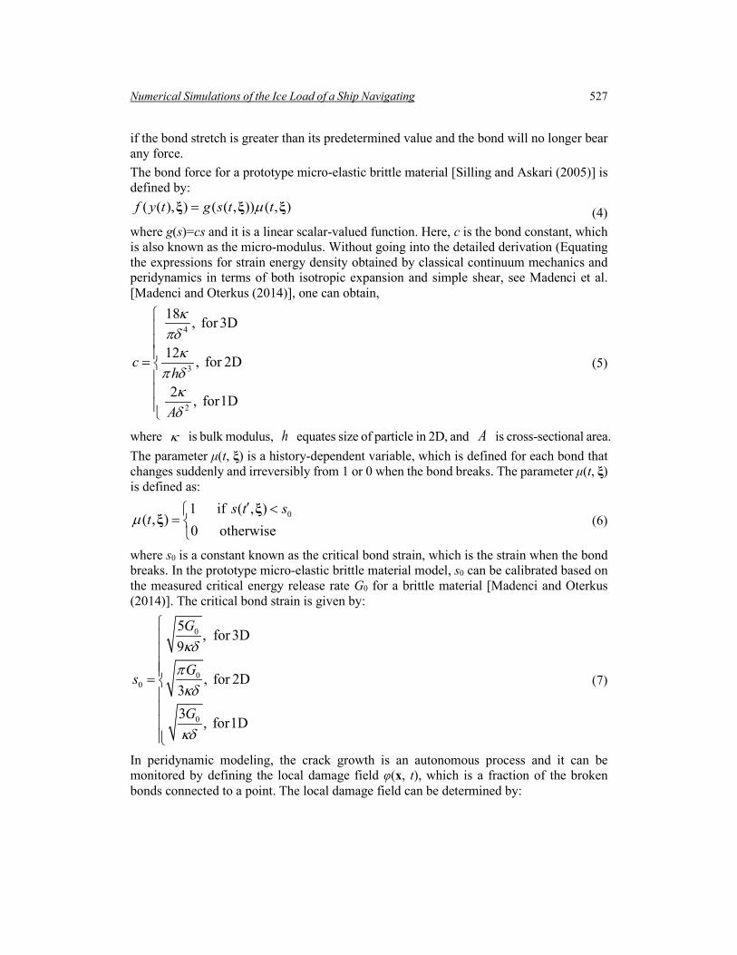
Fig. 2 shows that compressive strength and tensile strength has a similar trend except δ=3 mm, which has a jump at M=4.015 for tension case. Compared with values obtained from experiments, δ=1 mm and M=3.015, and δ=2 mm and M=4.015 agree well with experimental results [Schulson and Duval (2009)]. In this special case, the problem shows less “non-local” physical behavior, because the accuracy no longer increases with increasing horizon. Therefore, in practice, a sufficiently large horizon value can be chosen which does not show any significant non-local behavior, to make the computational time significantly decrease. M=3.015 is used in present model. One should note that in some cases, horizon can be used as a length scale parameter and can be adjusted in such a way that the required physical behavior can be accurately represented [Madenci and Oterkus (2014)]. Further study on the effect of the lattice size on critical strength as the horizon size stays constant M=3.015 is shown in Fig. 3. From Fig. 3, both compression and tension strengths are close to a stable value, except the lattice size is 17.5 mm (with values of 27501 and 5462 N showing more accurate). Therefore, the ratio of the characteristic scale to the lattice size should be no less than 4 (70/17.5) for getting reasonable results, however, additional studies may be required for this conclusion. One should note that the results obtained above are only applicable to three dimensional situations. For two-dimensional and one-dimensional problems, further studied need to be performed according to Eqs. (5) and (7).

530 CMES, vol.121, no.2, pp.523-550, 2019

Table 3: Errors for compression simulation cases (left) and tension simulation cases (right)

δ (mm)

M=δ/dx M=δ/dx 1.015 2.015 3.015 4.015 5.015 1.015 2.015 3.015 4.015 5.015

1 0.207 0.059 0.002 0.046 0.045 0.188 0.048 0.009 0.009 0.039 2 0.208 0.030 0.031 0.005 0.027 0.196 0.026 0.033 0.0003 0.019 3 0.208 0.017 0.056 0.011 0.062 0.196 0.027 0.064 0.078 0.002 4 0.208 0.059 0.034 0.026 0.017 0.194 0.062 0.088 0.029 0.022 5 0.207 0.138 0.109 0.062 0.050 0.194 0.132 0.113 0.068 0.056

Figure 3: Critical strength curve of uniaxial compressive and tensile test of ice used peridynamics

3.2 Micro-parameters of ice A large number of parameters such as the elastic modulus, Poisson’s ratio, viscosity, ultimate bending strength, and compressive strength are required in order to ensure that the constitutive model adequately captures the complex physics of ice. These parameters are essential to reflect the physical and mechanical properties of ice in the numerical simulations. It is crucial to accurately determine the values of these parameters by carrying out a series of tests. However, in order to demonstrate the viability of the peridynamic model in the absence of such test data, these parameters can be estimated by using the test data published in Ji et al. [Ji, Wang, Jie et al. (2011); Wang, Ning and Ji (2014)] for ice-covered waters in the Bohai Sea in winter. These test data were obtained from two typical model tests: (1) uniaxial compression test and (2) three-point bending test. Both of these tests were simulated in this study using the peridynamic model based on the assumption that ice is an isotropic prototype micro-elastic brittle material. The physical and mechanical properties of ice are defined by micro-parameters such as the micro-modulus c and critical bond strain s0. Still model test is an efficient approach to determine the micro-parameters of ice, where the micro-parameters are varied to cater for the macro properties of the specimens, which will improve the accuracy of the numerical


model. The readers may refer to Liu et al. [Liu, Xue, Lu et al. (2018)] for details on the simulation methods.

Figure 4: Bond force as a function of bond stretch for the ice material model (prototype micro-elastic brittle material model)

Fig. 4 shows the bond force as a function of the bond deformation for the ice material model with the following micro-parameters: E=1.8 GPa, S0c=0.003133, and S0b=0.000625. These parameters were used for subsequent studies, where the compressive strength and bending strength of the ice are 5.6 MPa and 1.125 MPa, respectively.

4 Simplifying assumptions 4.1 Gravitational and buoyancy forces A few assumptions need to be made in order to simplify the ship-ice interaction model. Firstly, it was assumed that the gravitational force is balanced by the buoyancy force of the ice sheet in calm waters. When the ship (icebreaker) is present, the ice sheet deviates from its equilibrium position due to imbalance of the gravitational and buoyancy forces, which will affect the motion of the ice sheet. It was assumed that the buoyancy force acting on the ice block is approximately linear to the change in position of the material point. Consequently, Δf, which is a function of the gravitational force density g, as well as the volume force density b of a material point will vary linearly with changes in the position of the material point. For example, assuming that the center coordinates of point x in the vertical direction is x with the waterline taken as the datum, Δf can be determined by:

( )

i w

i

i w w

if 2if 2

0.5 otherwise

g g x dxf g x dx

g g l dx

ρ ρρρ ρ

− + < −∆ = − >− + −

(9)

where ρi is the density of ice, ρw is the density of water, lw is the length of the material point immersed in the water, and dx is the scale of the material point.

ss0cs0b

g s( )

μ=1μ=0 μ=0

f

532 CMES, vol.121, no.2, pp.523-550, 2019

(a) Position of a material point to water surface.

(b) Gravity and buoyancy acting on a material point.

Figure 5: Schematic diagram of the effect of the gravitational and buoyancy forces

4.2 Ship-ice contact model The contact force model used in this study is defined by the repelling short-range force [Silling (2000)]. The force between two material points can be expressed as:

( ) ( )( ) ( )sh ( ) ( ) sh

sh( ) ( )

( , ) min 0, ( 1)2

j kj kj k

j k

cr

−− = − −

y yy yf y y

y y (10)

where csh is the short-range force constant and rsh is the critical distance. The short-range force is non-existent if the critical distance is exceeded. Here, csh=5⋅c while rsh=dx/2 [Madenci and Oterkus (2014)]. In this study, the ice material model (prototype micro-elastic brittle material model) has the dimensions of 16.0 m×16.0 m×1.0 m with 64×64×4 uniform discrete particles. The ice model consists of three levels of particles as the boundaries, more literatures about the boundary condition [Wildman and Gazonas (2013); Wang, Chen, Xu et al. (2017); Gu, Madenci and Zhang (2018)]. The ship-ice interaction was established with the ship bow model moving at a constant sailing speed of 3 kn. The time step size is 10-7 s. The ship-ice interactions were simulated using the peridynamic model and the results are shown in Fig. 6. The key characteristics of the ship-ice interactions such as indentations, radial cracks, bending of ice, and circumferential cracks can be obtained from the peridynamic model.


(a) 0.521 st = (b) 1.040 st = (c) 1.085 st =

(d) 1.216 st = (e) 1.302 st = (f) 2.605 st =

(g) 4.340 st =

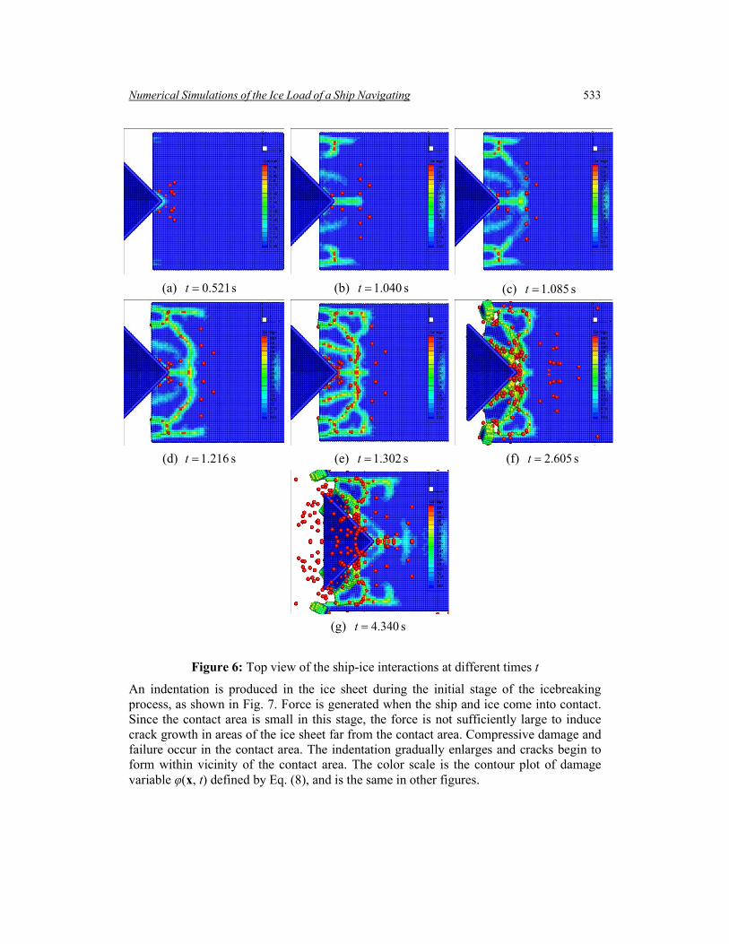
Figure 6: Top view of the ship-ice interactions at different times t

An indentation is produced in the ice sheet during the initial stage of the icebreaking process, as shown in Fig. 7. Force is generated when the ship and ice come into contact. Since the contact area is small in this stage, the force is not sufficiently large to induce crack growth in areas of the ice sheet far from the contact area. Compressive damage and failure occur in the contact area. The indentation gradually enlarges and cracks begin to form within vicinity of the contact area. The color scale is the contour plot of damage variable φ(x, t) defined by Eq. (8), and is the same in other figures.

534 CMES, vol.121, no.2, pp.523-550, 2019

Figure 7: Indentation and crack initiation within the contact area

Radial cracks begin to appear as the icebreaking process continues, as shown in Fig. 8. In this stage, the tensile strength of ice is lower than its compressive strength and thus, cracks begin to form at the lower surface of the ice sheet and the radial cracks propagate along with the ship motion.

Figure 8: Propagation of radial cracks in the ice sheet

As the radial cracks continue to develop in the ice sheet, the ice surface near the contact area is split into separate areas, forming wedge-shaped cantilevers. The force acting on the ice gradually increases until the ice sheet can no longer support the continuous bending of the cantilevers. The upper surface of the ice sheet is subjected to tensile loads whereas the lower surface of the ice sheet is subjected to compressive loads and therefore, circumferential cracks form on the upper surface. These circumferential cracks eventually penetrate through the ice sheet across its thickness, as shown in Fig. 9. One should note that this simulation of ship-ice interaction in the level ice with fixed boundaries, and the boundary regions of the ice plate contains three layers of material points on each edge which are fixed and free of deformation. These fixed boundaries have a substantial influence on the interaction process shown in Figs. 6, 8 and 9. However, for calculating ice load, it is reasonable to study the level ice with the size of the channel.


Figure 9: Growth of circumferential cracks in the ice sheet

5 Validation of the simulation results 5.1 Ship navigation in level ice In this study, the ice material model (prototype micro-elastic brittle material model) has the dimensions of 25.0 m×30.0 m×0.5 m with 200×240×4 uniform discrete particles. The ice model consists of three levels of particles as the boundaries. The principal dimensions of the selected icebreaker are 101.1 m×20.4 m×12.0 m and the depth of water needed to float the icebreaker (draught) is 7.5 m. A simplified ship bow model was developed in this study with the dimensions of 16 m×20.4 m×7.0 m and 51200 particles. The ship-ice interaction was established with the ship bow model moving at a constant sailing speed of 3 kn. The ice load F(t) is the summation of the short-range forces exerted on the material points of the bow. The load-time history curves are obtained based on the following equation:

( )

1 1( ) V

ni tns

sht = ⋅∑∑F f (11)

where F(t) is the ice load at time t, ns is the number of ship material points, ni(t) is the number of ice material points interacting with the ship material points at time t, fsh is the contact force density determined from Eq. (10), and V is the volume of the ice material points. Figs. 10 and 11 show the top view and side view of the ship navigating in level ice at different times t obtained from simulations using the peridynamic model, respectively.

(a) t=1.74 s (b) t=3.47 s (c) t=5.21 s

536 CMES, vol.121, no.2, pp.523-550, 2019

(d) t=6.95 s (e) t=8.68 s (f) t=10.42 s

(g) t=12.15 s (h) t=13.89 s (i) t=15.62 s

(j) t=17.36 s

Figure 10: Top view of the ship navigating in level ice at different times t

It can be observed from Figs. 10 and 11 that the level ice is broken into fragments and these ice fragments then drift away from the ship bow. In reality, the channel will be opened over a continuous period, but in this study, the ship-ice interactions are only considered within a small fraction of the period in which the icebreaking process takes place. Most of the time, the ship sails through the ice rubble or ice-free conditions, which results in impulsive ice loads. The simulation results shown in Figs. 10 and 11 conform well with the characteristics of the icebreaking process described above. It is evident that the cracks are fully developed at 1.74 s in the initial stage and the icebreaking process enters the following stage at 8.68 s. The ice loads imposed on the ship bow are rather low during this process.


(a) t = 1.74 s (b) t = 3.47 s (c) t = 5.21 s

(d) t = 6.95 s (e) t = 8.68 s (f) t = 10.42 s

(g) t = 12.15 s (h) t = 13.89 s (i) t = 15.62 s

(j) t = 17.36 s

Figure 11: Side view of the ship navigating in level ice at different times t

538 CMES, vol.121, no.2, pp.523-550, 2019

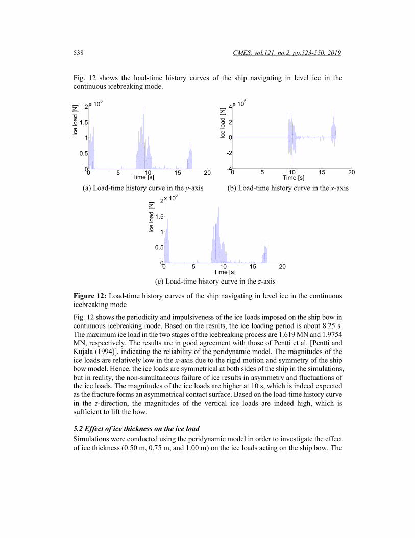
Fig. 12 shows the load-time history curves of the ship navigating in level ice in the continuous icebreaking mode.

(a) Load-time history curve in the y-axis (b) Load-time history curve in the x-axis

(c) Load-time history curve in the z-axis

Figure 12: Load-time history curves of the ship navigating in level ice in the continuous icebreaking mode

Fig. 12 shows the periodicity and impulsiveness of the ice loads imposed on the ship bow in continuous icebreaking mode. Based on the results, the ice loading period is about 8.25 s. The maximum ice load in the two stages of the icebreaking process are 1.619 MN and 1.9754 MN, respectively. The results are in good agreement with those of Pentti et al. [Pentti and Kujala (1994)], indicating the reliability of the peridynamic model. The magnitudes of the ice loads are relatively low in the x-axis due to the rigid motion and symmetry of the ship bow model. Hence, the ice loads are symmetrical at both sides of the ship in the simulations, but in reality, the non-simultaneous failure of ice results in asymmetry and fluctuations of the ice loads. The magnitudes of the ice loads are higher at 10 s, which is indeed expected as the fracture forms an asymmetrical contact surface. Based on the load-time history curve in the z-direction, the magnitudes of the vertical ice loads are indeed high, which is sufficient to lift the bow.

5.2 Effect of ice thickness on the ice load Simulations were conducted using the peridynamic model in order to investigate the effect of ice thickness (0.50 m, 0.75 m, and 1.00 m) on the ice loads acting on the ship bow. The

0 5 10 15 20 -4

-2

0

2

4 x 10 5

Time [s]

Ice

load

[N]

0 5 10 15 20 0

0.5

1

1.5

2 x 10 6

Time [s]

Ice

load

[N]

0 5 10 15 20 0

0.5

1

1.5

2 x 10 6

Time [s]

Ice

load

[N]


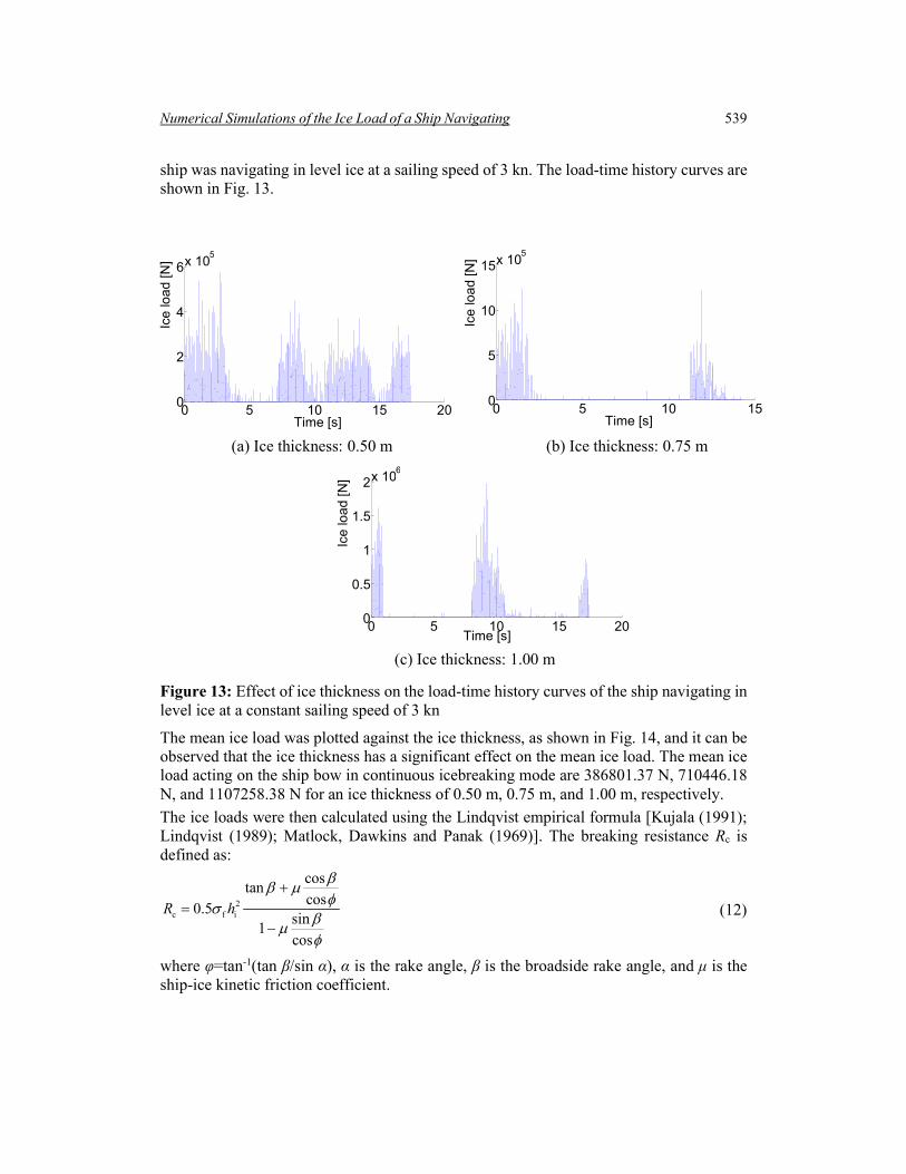
ship was navigating in level ice at a sailing speed of 3 kn. The load-time history curves are shown in Fig. 13.

(a) Ice thickness: 0.50 m (b) Ice thickness: 0.75 m

(c) Ice thickness: 1.00 m

Figure 13: Effect of ice thickness on the load-time history curves of the ship navigating in level ice at a constant sailing speed of 3 kn

The mean ice load was plotted against the ice thickness, as shown in Fig. 14, and it can be observed that the ice thickness has a significant effect on the mean ice load. The mean ice load acting on the ship bow in continuous icebreaking mode are 386801.37 N, 710446.18 N, and 1107258.38 N for an ice thickness of 0.50 m, 0.75 m, and 1.00 m, respectively. The ice loads were then calculated using the Lindqvist empirical formula [Kujala (1991); Lindqvist (1989); Matlock, Dawkins and Panak (1969)]. The breaking resistance Rc is defined as:

2c f i

costancos0.5

sin1cos

R h

ββ µφσ

βµφ

+=

− (12)

where φ=tan-1(tan β/sin α), α is the rake angle, β is the broadside rake angle, and μ is the ship-ice kinetic friction coefficient.

0 5 10 15 20 0

2

4

6 x 10 5

Time [s]

Ice

load

[N]

0 5 10 15 0

5

10

15 x 10 5

Time [s]

Ice

load

[N]

0 5 10 15 20 0

0.5

1

1.5

2 x 10 6

Time [s]

Ice

load

[N]

540 CMES, vol.121, no.2, pp.523-550, 2019

The bending resistance Rb can be expressed in terms of the ice thickness hi as follows: 1.5i

b f

2w

27 cos 1(tan )(1 )64 cos sin cos

12(1 )

hR BE

g

µ βσ φφ α φ

υ ρ

= + +

− (13)

where υ is the Poisson’s ratio, σf is the bending strength of ice, B is the breadth of ship, and ρw is the density of sea water. The submersion resistance Rs is defined as:

s w i tot( )R gh BKρ ρ= − (14)

++−−+

++

=αβ

ϕβαβ

µ 22 tan1

sin1coscos

tan4tan7.0

2TBTL

TBTBTK (15)

where ρi is the density of sea ice, htot is the thickness of ice and snow, T is the vertical distance between the water surface and lowest point of the ship hull (otherwise known as draft), and L is the length of the ship. The total resistance R is defined as:

c b si

1.4 9.4( ) 1 1V VR R R Rgh gL

= + + + +

(16)

where V is velocity of the ship. In current study, much less ice sliding force is present in such a short simulation. Therefore, Rs should not be included in next calculation. Because Lindqvist assumed that Rs is calculated when 70% of the ship is covered by broken ice, that is why there is the parameter 0.7 in Eq. (15). The values of the parameters used in the Lindqvist empirical formula are presented in Tab. 5.

Table 4: Major computational parameters used in Lindqvist empirical formula

ρi μ σf L α

920 kg/m3 0.15 1.125 MPa 101.1 m 20°

β ρw T B υ 20° 1035 kg/m3

7.5 m 20.4 m 0.33

Table 5: Comparison between mean ice loads determined from the peridynamic model and Lindqvist empirical formula

Ice thickness (m)

Results using peridynamics (N)

Results using Lindqvist formula (N) Error

0.50 315828.46 386801.37 18.35% 0.75 650577.60 710446.18 8.43% 1.00 988055.98 1107258.38 10.77%


The mean ice loads determined from the peridynamic model and Lindqvist empirical formula are summarized in Tab. 6. Fig. 14 shows the mean ice loads determined from the peridynamic model and Lindqvist empirical formula plotted against the ice thickness. It can be seen that the mean ice load is almost linearly depended on the square of the ice thickness when the ship is traveling at a speed of 3 kn. The mean ice load at an ice thickness of 1.00 m is 3.13 times higher than that at an ice thickness of 0.50 m, indicating that ice thickness is indeed a factor that significantly affects the ice load. The mean ice loads determined from the peridynamic model are consistent with those determined from the Lindqvist empirical formula, which proves the viability of the peridynamic model. The difference between the results obtained from the peridynamic model and Lindqvist empirical formula may be due to the lack of consideration on the role of water and frictional effects between the ship and ice in the peridynamic model.

Figure 14: Effect of ice thickness on the mean ice load determined from the peridynamic model and Lindqvist empirical formula

5.3 Effect of sailing speed on the ice load In order to investigate the effect of sailing speed on the ice loads imposed on the ship bow, the sailing speed of the ship was varied in the simulations (3, 4, 5, 6, 7, and 8 kn) while the thickness of the ice sheet was fixed at 0.50 m. The load-time history curves are shown in Fig. 15.

542 CMES, vol.121, no.2, pp.523-550, 2019

(a) Sailing speed: 3 kn (b) Sailing speed: 4 kn

(c) Sailing speed: 5 kn (d) Sailing speed: 6 kn

(e) Sailing speed: 7 kn (f) Sailing speed: 8 kn

Figure 15: Effect of sailing speed on the load-time history curves of the ship navigating in level ice with a constant thickness of 0.50 m

Fig. 16 shows the mean ice load plotted against the sailing speed and it can be observed that the mean ice load slightly increases when the sailing speed of the ship is increased from 3 to 5 kn. The mean ice load significantly increases when the sailing speed is increased beyond 5 kn.

0 2 4 6 8 10 0

0.5

1

1.5

2 x 10 6

Time [s]

Ice

load

[N]

0 5 10 15 0

2

4

6

8 x 10 5

Time [s]

Ice

forc

e [N

]

0 5 10 15 20 0

2

4

6 x 10 5

Time [s]

Ice

load

[N]

0 5 10 15 20 0

2

4

6

8 x 10 5

Time [s]

Ice

load

[N]

0 2 4 6 8 10 0

5

10 x 10 5

Time [s]

Ice

load

[N]

0 2 4 6 8 10 0

5

10

15 x 10 5

Time [s]

Ice

load

[N]


Figure 16: Plot of mean ice force against speed

5.4 Effect of ice properties on the ice load The compressive strength and tensile strength of the materials were determined based on the critical stretch of the bond in tensile and compression, respectively. It is known that the elastic modulus of ice is related to its compressive strength and tensile strength. Hence, if there are changes in the elastic modulus of ice, there will be changes in the bond critical stretch. For this reason, the effects of elastic modulus and compressive strength of ice on the ice loads were investigated in this study and three cases were considered: Case I, Case II, and Case III. The ship was navigating in level ice with a thickness of 0.5 m and a sailing speed of 3 kn. In Case I, the elastic modulus of ice was varied at 1.8, 2.0, 2.2, 2.4, 2.6, 2.8, and 3.0 GPa and its effect on the mean ice load acting on the ship bow are shown in Fig. 17.

Figure 17: Effect of elastic modulus of ice on the mean ice load determined from the peridynamic model and peridynamic model with linear fit

544 CMES, vol.121, no.2, pp.523-550, 2019

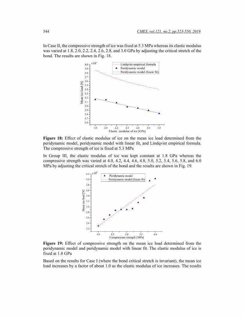
In Case II, the compressive strength of ice was fixed at 5.3 MPa whereas its elastic modulus was varied at 1.8, 2.0, 2.2, 2.4, 2.6, 2.8, and 3.0 GPa by adjusting the critical stretch of the bond. The results are shown in Fig. 18.

Figure 18: Effect of elastic modulus of ice on the mean ice load determined from the peridynamic model, peridynamic model with linear fit, and Lindqvist empirical formula. The compressive strength of ice is fixed at 5.3 MPa

In Group III, the elastic modulus of ice was kept constant at 1.8 GPa whereas the compressive strength was varied at 4.0, 4.2, 4.4, 4.6, 4.8, 5.0, 5.2, 5.4, 5.6, 5.8, and 6.0 MPa by adjusting the critical stretch of the bond and the results are shown in Fig. 19.

Figure 19: Effect of compressive strength on the mean ice load determined from the peridynamic model and peridynamic model with linear fit. The elastic modulus of ice is fixed at 1.8 GPa

Based on the results for Case I (where the bond critical stretch is invariant), the mean ice load increases by a factor of about 1.0 as the elastic modulus of ice increases. The results


for Case II (where only the elastic modulus of ice is varied while its compressive strength is kept constant) show that there are no significant variations in the mean ice load as the elastic modulus of ice increases. This is also confirmed by the results obtained from the Lindqvist empirical formula. The results for Case III (where the compressive strength is varied while the elastic modulus of ice is kept constant) show that the mean ice load increases with an increase in the compressive strength. The following correlations were obtained by applying linear fitting to the data for each case, which can be used to predict the mean ice load acting on the ship bow as a function of the elastic modulus or compressive strength of ice. Case I:

0.000131554 101891F E= + (σc=εcE) (17) Case II:

0.000029611 371664F E= − + (σc=5.3 MPa) (18) Case III:

c0.076331 75902F σ= − (E=1.8 GPa) (19) For Case II, the value of the slope is -0.029611 with the unit of meganewtons (MN). This indicates that the elastic modulus of ice affects the mean ice load by ~3.0% if the compressive strength of ice is constant. For Case III, the value of the slope is 0.076331, with ~2.6 times of the effect of elastic modulus. The results presented in this section demonstrate the effect of elastic modulus and compressive strength of ice on the ice loads imposed on the ship bow. In general, the compressive strength of ice has a higher contribution to the ice load.

6 Conclusions In this study, a model was developed based on peridynamic theory in order to simulate the ship-ice interactions of a ship navigating in level ice in continuous icebreaking mode. The ice loads and key characteristics of the icebreaking process were captured at different ice thicknesses and sailing speeds. The effect of the physical and mechanical properties of ice on the ice loads was also investigated. The following conclusions were drawn based on the simulation results: Convergence study showed the different ratios of the horizon to lattice size show similar trend of change in both compression and tension. The horizon size of 3.015 lattice size give the most accurate result in compression; however, the horizon size of 4.015 lattices shows the most accurate result in tension. Additionally, given the horizon size of 3.015 lattice size, the ratio of the size of model to lattice size no less than four gives more accurate results. It can be generalized that the number of particles on any dimension should be more than the ratio of the horizon to lattice size. The mean ice load increases almost linearly depended on the square of the ice thickness. The mean ice load at an ice thickness of 1.00 m is 3.13 times higher than that at an ice thickness of 0.50 m.

546 CMES, vol.121, no.2, pp.523-550, 2019

The mean ice load slightly increases as the sailing speed of the ship is increased from 3 to 5 kn. However, the ice load increases significantly when the sailing speed is increased beyond 5 kn. Within the peridynamic framework, it is found that the compressive strength of ice has a higher contribution to the mean ice load about 2.6 times of the elastic modulus of ice.

Acknowledgment: This project has received funding from the European Union’s Horizon 2020 research and innovation programme under grant agreement (Grant No. 2017YFE0111400); the National Key R&D Program Strategic International Science and Technology Innovation Cooperation Key Specialities (Grant No. 2016YFE0202700); the National Natural Science Foundation of China (Grant Nos. 51579054 and 51639004), and the Ministry of Industry and Information Technology’s High-tech Ship Research Project (Grant No. 2017-614). Mr. Renwei Liu is supported by a two-year visiting student fellowship in University of California, Berkeley from Chinese Scholar Council (Grant No. 201706680104), and this support is gratefully acknowledged. The authors also graciously acknowledge Professor Shaofan Li of University of California, Berkeley and Fei Han of Dalian University of Technology for their guidance and fruitful discussion regarding this work.

References Arttu, P.; Jukka, T. (2009): 3D discrete numerical modelling of ridge keel punch through tests. Cold Regions Science and Technology, vol. 56, no. 1, pp. 18-29. Benz, W.; Asphaug, E. (1994): Simulations of brittle solids using smooth particle hydrodynamics. Computer Physics Communications, vol. 87, no. 1, pp. 253-265. Bobaru, F.; Yang, M.; Alves, L. F.; Silling, S. A.; Askari, E. et al. (2009): Convergence, adaptive refinement; scaling in 1D peridynamics. International Journal for Numerical Methods in Engineering, vol. 77, no. 6, pp. 852-877. Cheng, Z.; Zhang, G.; Wang, Y.; Bobaru, F. (2015): A peridynamic model for dynamic fracture in functionally graded materials. Composite Structures, vol. 133, pp. 529-546. Daley, C. G. (1991). Ice edge contact-A brittle failure process model. Loads, vol. 144, no. 100, pp. 1-92. Das, J. (2017): Modeling and validation of simulation results of an ice beam in four-point bending using smoothed particle hydrodynamics. International Journal of Offshore and Polar Engineering, vol. 27, no. 1, pp. 82-89. Deb, D.; Pramanik, R. (2013): Failure process of brittle rock using smoothed particle hydrodynamics. Journal of Engineering Mechanics, vol. 139, no. 11, pp. 1551-1565. Di, S.; Xue, Y.; Bai, X.; Wang, Q. (2017): Effects of model size and particle size on the response of sea-ice samples created with a hexagonal-close-packing pattern in discrete-element method simulations. Particuology, vol. 36, no. 2018, pp. 106-113. Enkvist, E. (1972): On the Ice Resistance Encountered by Ships Operating in the Continuous Mode of Icebreaking (No. 24). Swedish Academy of Engineering Sciences in Finland. Fan, H.; Li, S. (2017): A Peridynamics-SPH modeling and simulation of blast fragmentation of soil under buried explosive loads. Computer Methods in Applied


Mechanics and Engineering, vol. 318, pp. 349-381. Freimanis, A.; Paeglitis, A. (2017): Mesh sensitivity in peridynamic quasi-static simulations. Procedia Engineering, vol. 172, pp. 284-291. Gerstle, W. H. (2015): Introduction to Practical Peridynamics: Computational Solid Mechanics Without Stress and Strain, vol. 1. World Scientific Publishing Company. Gu, X.; Madenci, E.; Zhang, Q. (2018): Revisit of non-ordinary state-based peridynamics. Engineering Fracture Mechanics, vol. 190, pp. 31-52. Gu, X.; Zhang, Q.; Huang, D.; Yv, Y. (2016): Wave dispersion analysis and simulation method for concrete SHPB test in peridynamics. Engineering Fracture Mechanics, vol. 160, no. 160, pp. 124-137. Han, D.; Zhang, Y.; Wang, Q.; Lu, W.; Jia, B. (2018): The review of the bond-based peridynamics modeling. Journal of Micromechanics and Molecular Physics, vol. 4, no. 1, 1830001. Han, F.; Lubineau, G.; Yan, A.; Askari, A. (2016): A morphing approach to couple state-based peridynamics with classical continuum mechanics. Computer Methods in Applied Mechanics and Engineering, vol. 301, pp. 336-358. Han, L.; Feng, L. I.; Yue, Q. (2007): Simulation of the whole failure process by FEM during ice-conical structures interaction. China Offshore Platform. Huang, Y.; Ma, J.; Tian, Y. (2013): Model tests of four-legged jacket platforms in ice: Part 1. Model tests and results. Cold Regions Science and Technology, vol. 95, no. 11, pp. 74-85. Karulin, E. B.; Karulina, M. M. (2011): Numerical and physical simulations of moored tanker behaviour. Ships and Offshore Structures, vol. 6, no. 3, pp. 179-184. Kheisin, D. E.; Popov, Y. N. (1973): Ice navigation qualities of ships. Icebreakers. Kim, M. C.; Lee, S. K.; Lee, W. J.; Wang, J. Y. (2013): Numerical and experimental investigation of the resistance performance of an icebreaking cargo vessel in pack ice conditions. International Journal of Naval Architecture and Ocean Engineering, vol. 5, no. 1, pp. 116-131. Kim, W. J.; Kim, S. P.; Sim, I. H.; Hur, J. W.; Kim, H. S. et al. (2015): Ice resistance estimation and comparison the results with model test. Twenty-fifth International Ocean and Polar Engineering Conference. Kolari, K.; Kuutti, J.; Kurkela, J. (2009). FE-simulation of continuous ice failure based on model update technique. Proceedings of the International Conference on Port and Ocean Engineering Under Arctic Conditions. Konno, A.; Nakane, A.; Kanamori, S. (2013): Validation of numerical estimation of brash ice channel resistance with model test. Proceedings of the International Conference on Port and Ocean Engineering Under Arctic Conditions. Kujala, P. (1991): Safety of ice-strengthened ship hulls in the Baltic Sea. Safety. Kujala, P. (1994): On the statistics of ice loads on ship hull in the Baltic. Icebreaking. Kujala, P.; Vuorio, J. (1986): Results and Statistical Analysis of Ice Load Measurements on Board Icebreaker Sisu in Winters 1979 to 1985 (Research Report No. 43). Winter

548 CMES, vol.121, no.2, pp.523-550, 2019

Navigation Research Board. Kwok, R.; Cunningham, G. F. (2012): Deformation of the Arctic Ocean ice cover after the 2007 record minimum in summer ice extent. Cold Regions Science and Technology, vol. 76-77, no. 1, pp. 17-23. Lai, X.; Liu, L.; Li, S.; Zeleke, M.; Liu, Q. et al. (2017): A non-ordinary state-based peridynamics modeling of fractures in quasi-brittle materials. International Journal of Impact Engineering, vol. 111. Leira, B.; Børsheim, L.; Espeland, Ø.; Amdahl, J. (2009): Ice-load estimation for a ship hull based on continuous response monitoring. Proceedings of the Institution of Mechanical Engineers Part M Journal of Engineering for the Maritime Environment, vol. 223, no. 4, pp. 529-540. Li, S.; Liu, W. K. (2002): Meshfree and particle methods and their applications. Applied Mechanics Reviews, vol. 55, no. 1, pp. 1-34. Libersky, L. D.; Petschek, A. G. (1991): Smooth particle hydrodynamics with strength of materials. Lecture Notes in Physics, vol. 395, pp. 248-257. Lindqvist, G. (1989): A straightforward method for calculation of ice resistance of ships. Performance. Liu, M.; Wang, Q.; Lu, W. (2016): Peridynamic simulation of brittle-ice crushed by a vertical structure. International Journal of Naval Architecture and Ocean Engineering, vol. 9, no. 2. Liu, R. W.; Xue, Y. Z.; Lu, X. K.; Cheng, W. X. (2018): Simulation of ship navigation in ice rubble based on peridynamics. Ocean Engineering, vol. 148, pp. 286-298. Lubbad, R.; Løset, S. (2011): A numerical model for real-time simulation of ship-ice interaction. Cold Regions Science and Technology, vol. 65, no. 2, pp. 111-127. Luo, W. Z.; Guo, C. Y.; Wu, T. C.; Su, Y. M. (2018): Experimental research on resistance and motion attitude variation of ship-wave-ice interaction in marginal ice zones. Marine Structures, vol. 58, pp. 399-415. Madenci, E.; Oterkus, E. (2014): Peridynamic Theory and Its Applications. Springer New York. Matlock, H.; Dawkins, W.; Panak, J. (1969): A modal for the prediction of ice-structure internation. Philosophy East and West, vol. 22, no. 2. Metrikin, I.; Løset, S. (2013): Nonsmooth 3D discrete element simulation of a drillship in discontinuous ice. Proceedings of the International Conference on Port and Ocean Engineering Under Arctic Conditions. Metrikin, I.; Løset, S.; Jenssen, N. A.; Kerkeni, S. (2013): Numerical simulation of dynamic positioning in ice. Marine Technology Society Journal, vol. 47, no. 47, pp. 14-30. Ni, T.; Zhu, Q. Z.; Zhao, L. Y.; Li, P. F. (2017): Peridynamic simulation of fracture in quasi brittle solids using irregular finite element mesh. Engineering Fracture Mechanics, vol. 188, pp. 320-343. Nylandsted, J.; Jäättelä, M.; Hoffmann, E. K.; Pedersen, S. F. (2003): Finite element modelling and simulation of indentation testing: a bibliography (1990-2002). Engineering


Computations, vol. 21, no. 1, pp. 23-52, 30. Paavilainen, J.; Tuhkuri, J. (2013): Pressure distributions and force chains during simulated ice rubbling against sloped structures. Cold Regions Science and Technology, vol. 85, pp. 157-174. Premachandran, R.; Horii, H. (1994): A micromechanics-based constitutive model of polycrystalline ice and FEM analysis for prediction of ice forces. Cold Regions Science and Technology, vol. 23, no. 1, pp. 19-39. Rabczuk, T.; Ren, H. (2017): A peridynamics formulation for quasi-static fracture and contact in rock. Engineering Geology, vol. 225, pp. 42-48. Ranta, J.; Polojärvi, A.; Tuhkuri, J. (2018): Ice loads on inclined marine structures-Virtual experiments on ice failure process evolution. Marine Structures, vol. 57, pp. 72-86. Ren, H.; Zhuang, X.; Rabczuk, T. (2017): Dual-horizon peridynamics: a stable solution to varying horizons. Computer Methods in Applied Mechanics and Engineering, vol. 318, pp. 762-782. Ren, H.; Zhuang; X.; Cai, Y.; Rabczuk, T. (2016): Dual-horizon peridynamics. International Journal for Numerical Methods in Engineering, vol. 108, no. 12, pp. 1451-1476. Schulson, E. M.; Duval, P. (2009): Creep and Fracture of Ice, pp. 213. Cambridge University Press. Ji, S. Y.; Wang, A. L.; Jie, S. U.; Yue, Q. J. (2011): Experimental studies and characteristics analysis of sea ice flexural strength around the Bohai Sea. Shuikexue Jinzhan/Advances in Water Science, vol. 22, no. 2, pp. 266-272. Silling, S. A. (2000): Reformulation of elasticity theory for discontinuities and long-range forces. Journal of the Mechanics and Physics of Solids, vol. 48, no. 1, pp. 175-209. Silling, S. A.; Askari, E. (2005): A meshfree method based on the peridynamic model of solid mechanics. Computers and Structures, vol. 83, no. 17, pp. 1526-1535. Stockstill, R. L.; Daly, S. F.; Hopkins, M. A. (2009): Modeling floating objects at river structures. Journal of Hydraulic Engineering, vol. 135, no. 135, pp. 403-414. Varsta, P. (1983): On the Mechanics of Ice Load on Ships in Level Ice in the Baltic Sea. VTT Technical Research Centre of Finland. Vuorio, J.; Riska, K.; Varsta, P. (1979): Long term measurements of ice pressure and ice induced stresses on the icebreaker sisu in winter 1978. Icebreakers. Wang, A. L.; Ning, X. U.; Ji, S. Y. (2014): Characteristics of sea ice uniaxial compressive strength around the coast of Bohai Sea. Ocean Engineering, vol. 32, no. 4, pp. 82-88. Wang, L.; Chen, Y.; Xu, J.; Wang, J. (2017): Transmitting boundary conditions for 1D peridynamics. International Journal for Numerical Methods in Engineering, vol. 110, no. 4, pp. 379-400. Wang, Q.; Wang, Y.; Zan, Y.; Lu, W.; Bai, X. et al. (2017): Peridynamics simulation of the fragmentation of ice cover by blast loads of an underwater explosion. Journal of Marine Science and Technology, no. 5, pp. 1-15. Wang, Y.; Zhou, X.; Wang, Y.; Shou, Y. (2018): A 3-D conjugated bond-pair-based

550 CMES, vol.121, no.2, pp.523-550, 2019

peridynamic formulation for initiation and propagation of cracks in brittle solids. International Journal of Solids and Structures, vol. 134, pp. 89-115. Wildman, R. A.; Gazonas, G. A. (2013): A perfectly matched layer for peridynamics in two dimensions. Journal of Mechanics of Materials and Structures, vol. 7, no. 8, pp. 765-781. Xue, H. (2016). Investigation of ice-PVC separation under flexural loading using FEM analysis. International Journal of Multiphysics, vol. 10, no. 3, pp. 247-264. Ye, L. Y.; Wang, C.; Chang, X.; Zhang, H. Y. (2017): Propeller-ice contact modeling with peridynamics. Ocean Engineering, vol. 139, pp. 54-64. Zhang, J. N.; Shang, Y. C.; Zhang, L. (2013): Ice resistance model test technology for 110K tanker adopting FSICR ice class IA. Advanced Materials Research, vol. 779-780, pp. 1117-1123. Zhang, N.; Zheng, X.; Ma, Q. (2017): Updated smoothed particle hydrodynamics for simulating bending and compression failure progress of ice. Water, vol. 9, no. 11, pp. 882. Zhang, Z. H.; Wang, C.; Gu, J. N.; Miao, T.; Wang, L. F. et al. (2012): Measurement method in model test of ice breaking by air cushion vehicle. Applied Mechanics and Materials, vol. 204-208, pp. 4694-4697.

numerical simulations of the ice load of a ship navigating...

Documents