sr237 mixture of normals probit models - federal … · favor mixture of normals probit models over...

Federal Reserve Bank of MinneapolisResearch Department Staff Report 237

August 1997

Mixture of Normals Probit Models

John Geweke*

University of Minnesotaand Federal Reserve Bank of Minneapolis

Michael Keane*

University of Minnesotaand Federal Reserve Bank of Minneapolis

ABSTRACT

This paper generalizes the normal probit model of dichotomous choice by introducing mixtures of normalsdistributions for the disturbance term. By mixing on both the mean and variance parameters and byincreasing the number of distributions in the mixture these models effectively remove the normalityassumption and are much closer to semiparametric models. When a Bayesian approach is taken, there isan exact finite-sample distribution theory for the choice probability conditional on the covariates. Thepaper uses artificial data to show how posterior odds ratios can discriminate between normal andnonnormal distributions in probit models. The method is also applied to female labor force participationdecisions in a sample with 1,555 observations from the PSID. In this application, Bayes factors stronglyfavor mixture of normals probit models over the conventional probit model, and the most favored modelshave mixtures of four normal distributions for the disturbance term.

JEL classification: Primary, C25; secondary, C11Keywords: Discrete choice, Markov chain Monte Carlo, Normal mixture

*Geweke wishes to acknowledge financial support from National Science Foundation grant SBR-9514865, Keane fromNSF grant SBR-9511186. We thank the editor, Robin Carter, Daniel Houser, and seminar participants at theUniversity of Western Ontario for comments on an earlier draft, but blame only each other for remaining errors.We thank John Landon-Lane and Lance Schibilla for research assistance. The views expressed herein are those ofthe authors and not necessarily those of the Federal Reserve Bank of Minneapolis or the Federal Reserve System.

1

1. Introduction

In econometric specifications of dichotomous choice models, the probit and logit

specifications are commonly used. Other specifications have been suggested (Maddala

1983, pp. 27–32; Aldrich and Nelson 1984), but in econometric applications, the probit

and logit specifications have been used almost exclusively. The probit model is easy to

use, and the logit specification is even more tractable. Because the probit specification can

be made free of the problem of independence of irrelevant alternatives (Hausman and

McFadden 1984) when moving from dichotomous to polytomous choice, whereas the logit

specification cannot, the probit model has become a mainstay in econometrics, and it is

likely to remain one.

It is widely appreciated that any misspecification of functional form in a dichotomous

choice model will lead to inconsistent estimates of conditional choice probabilities. In

particular, if a probit specification is maintained when a different specification is true,

misleading inferences about conditional choice probabilities and the effects of changes in

covariates on these probabilities may result. In this paper, we consider strict

generalizations of the probit specification that remain within the class of linear dichotomous

choice models:P dt = 1( ) = P ′β x t + ε t > 0( )

where dt is the choice indicator, x t is a vector of covariates, and ε t is an i.i.d. disturbance.

Our approach is fully parametric and Bayesian. This approach permits us to obtain explicit

evaluations of P dt = 1x t = x*( ) for any x* , which are ultimately the focus of any

application, and makes it possible to compare alternative generalizations with each other as

well as with the conventional probit model. These evaluations and comparisons can, in

principle, be accomplished with all Bayesian approaches to dichotomous choice. (See, for

example, Zellner and Rossi 1984; Albert and Chib 1993; Koop and Poirier 1993.)

However, recent developments in numerical methods have greatly simplified the

computation of posterior moments and Bayes factors. The class of specifications taken up

here is the mixture of normals distribution, in which

p ε( ) = 2π( )−1 2 pjhj1 2 exp −.5hj ε − α j( )2[ ]j =1

m∑ .

The generation of the shock may be described by first drawing from one of m specifiednormal distributions, with probabilities p1,K, pm , and then drawing the shock ε from that

distribution.

There is a large literature in econometric theory that has taken a semiparametric

approach to this problem by dealing with consistent estimation of β and making regularity

2

assumptions about the distribution of the shock rather than specifying it. The development

of this approach includes Cosslett (1983), Manski (1985), Gallant and Nychka (1987),

Powell, Stock, and Stoker (1989), Horowitz (1992), Ichimura (1993), and Klein and

Spady (1993). Lewbel (1997) extends this approach to consistent estimation of moments

of ε . This approach and the one taken here are complementary. Both break free of the

normality assumption of the probit model. On the one hand, the semiparametric approach

introduces a series of approximations that yields consistent estimates of covariate

coefficients given weak assumptions (for example, differentiability of the density function)

about the shock distribution, whereas we make no claim that the mixture of normals family

will similarly accommodate all such distributions. On the other hand, our method leads

directly to exact inference for P dt = 1x t = x*( ) , which the semiparametric approach does

not do even asymptotically.

The organization of the paper is simple. The next section describes the mixture of

normals probit model, beginning by extending the treatment of the probit model by Albert

and Chib (1993) and moving through to the development of a Markov chain Monte Carlo

posterior simulator and the evaluation of the marginal likelihood. Experiments with

artificial data provide some evidence on the ability of different models within the class to

cope with alternative shock distributions. These are reported in Section 3. A substantive

example pertaining to women’s labor force participation, which uses a subset of the Panel

Study of Income Dynamics (PSID) with 1,555 observations, is presented in Section 4. In

this example, the conventional probit model is overwhelmingly rejected in favor of the

mixture of normals probit model; several members of the mixture family have low Bayes

factors relative to one another, including mixtures of as many as 5 normals with 13 free

parameters describing the shape of the shock distribution. Some fairly obvious extensions

of this work are mentioned in the concluding section.

2. Bayesian inference for probit models

In the probit model, the observables are

′Xk ×T

= x1,K,xT[ ] and ′d = d1,K,dT( ) , dt = 0

or 1. The relationships of interest are(2.1)

yt = ′β x t + ε t , dt = χ 0,∞[ ) yt( ) t = 1,K,T( )

where the indicator function χS z( ) = 1 if z ∈S and χS z( ) = 0 if z ∉S . Let ′y = y1,K, yT( ).

3

2.1 Conventional probit model

In the conventional probit model,

(2.2) ε t X ~IID

N 0, 1( )and it is convenient to complete this model with the prior distribution β ~ N β , Hβ

−1( ),

where β ∈Rk and Hβ is a k × k positive definite precision matrix:

(2.3) p β( ) = 2π( )−k 2 Hβ1 2

exp −.5 β − β( )′Ηβ β − β( )

.

Albert and Chib (1993) develop a Gibbs sampling algorithm for Bayesian inference in

this model. From (2.1) and (2.2),

p d, yβ ,X( ) = p yβ ,X( )p d y( )(2.4) = 2π( )−T 2 exp −.5 y − Xβ( ) y − Xβ( )[ ] dtχ 0,∞[ ) yt( ) + 1 − dt( )χ −∞,0( ) yt( )[ ]t =1

T∏(2.5) = ( ) − − ′( )[ ] ( ) + −( ) ( )[ ]−

∞[ ) −∞( )=∏ 2 5 11 2 2

0 01π β χ χexp . ˜ ˜ ˜

, ,y d y d yt t t t t tt

Tx .

The joint posterior density for β and y is p β , y d,X( ) ∝ p d, yβ ,X( )p β( ) . When we

take the product of the joint density (2.4) and the prior density (2.3) and examine the kernel

of this expression in β ,

(2.6) β β β ββ β β β β˜, ~ N , , , ˜y X H H H X X H H X y( ) ( ) = + ′ = + ′( )− −1 1 .

Taking p d, yβ ,X( ) in the form (2.5), we have the T conditionally independent

distributions

(2.7) yt d,β ,X( ) = yt dt ,β ,x t( ) ~ N ′β x t , 1( ) subject to yt ≥ 0 if dt = 1 and yt < 0 if dt = 0 .

Beginning from an arbitrary point β 0( ) ∈Rk , we construct the sequence β r r( ) ( ){ }, y by

drawing sequentially from the T distributions in (2.7) and the distribution (2.6). (In all

results reported subsequently for this model, β 0( ) ~ N β , H−1( ) .) Given any point β *, y*( )in the support of p β , y d,X( ) and any subset A of the support with positive Lebesgue

measure, the probability of moving from β *, y*( ) into A in one iteration of this algorithm is

strictly positive. Therefore, the process β r r( ) ( ){ }, y is ergodic (Tierney 1994; Geweke

1997a, Section 3.3), which implies that if E g β( )d,X[ ] exists, then R m

m

M− ( )= ( )∑1

1g β

a s. . → E g β( )d,X[ ].

2.2 Mixture of normals probit model

In the mixture of normals probit model,

(2.8) ε α η α α αt tj j j tj

m

mm

mme h h h= +( ) ′ = ( ) ∈ ′ = ( ) ∈−

= +∑ 1 2

1 1 1, , , R , , , RK Kh

(2.9) ηt X ~IID

N 0, 1( ) .

4

The random vectors ′et = et1,K,etm( ) are i.i.d., each with a multinomial distribution with

parameters pJ = P etj = 1( ) j = 1,K,m( ) :

(2.10) e pt

IID

m m mp p p p S~ MN , , , , ,1 1K K( ) ′ = ( ) ∈where Sm is the unit simplex in Rm .

Without further restrictions, the model is clearly unidentified in the sense that morethan one set of values of the parameters in (2.1) and (2.8)–(2.10) imply the same p d X( ) .

Three specific identified versions of the model are of interest, each consisting of a set of

further restrictions on (2.1) and (2.8)–(2.10).

In the full mixture of normals model,

(i) rank X( ) = k and ′a ′X ≠ 1,K,1( ) for any k ×1 vector a;(ii) pj > 0 ∀ j ;

(iii) the support of ′β x t is a set of positive Lebesgue measure;

(iv) either(a) α j −1 < α j j = 2,K,m( ) or

(b) hj −1 < hj j = 2,K,m( ); and

(v) hj* = 1 for some j* .

In the scale mixture of normals model, α j = 0 j = 1,K,m( ), X may (and generally does)

include an intercept, and (iv-b) obtains. In the mean mixture of normals model, hj = 1

j = 1,K,m( ) and (iv-a) obtains. The orderings in (iv) are labeling restrictions that prevent

interchanging the components of the mixture; obviously, other labeling restrictions are

possible.

For Bayesian inference, it is convenient to complete the model with independent prior

distributions for β , α , h, and p. The prior distribution for β is (2.3). Except in the

scale mixture of normals model, α ~ N α, Hα−1( ), where α ∈Rm and Hα is an m × m

positive definite matrix:

(2.11) p α( ) = 2π( )−m 2 Hα1 2

exp −.5 α − α( )′Hα α − α( )

subject to (iv-a) in the mean mixture of normals model and in the full mixture of normals

model if (iv-b) is not invoked.

Except in the mean mixture of normals model, s j2hj ~ χ 2 ν j( ) j ≠ j*( ), where s j

2 > 0

and ν j > 0 . If (iv-b) is not imposed, then the prior density of h is

(2.12) p exp ., *h( ) = ( )[ ] ( ) −( )− −( )

= ≠∏ 2 2 52 1

2 2 2 2 2

1

ν ν ννj j j

j j j j jj j j

ms h s hΓ .

If (iv-b) is imposed, then the support is truncated accordingly, and the normalization

constant must be adjusted.Finally, p p( ) ~ Beta r( ), r ∈R+

m:

5

(2.13) p p( ) = Γ r jj =1

m∑( ) Γ r j( )j =1

m∏[ ] pj

rj −1( )j =1

m∏ .

Since the likelihood function

(2.14) p dβ ,α,h,p,X( ) = dt pjΦ hj1 2 α j + ′β x t( )[ ]j =1

m∑t =1

T∏+ 1 − dt( ) 1 − pjΦ hj

1 2 α j + ′β x t( )[ ]j =1

m∑{ }is bounded between zero and one,(2.15) p dβ ,α,h,p,X( )p β( )p α( )p h( )p p( )

is finitely integrable over its support, and, consequently, the posterior distributionp β ,α,h,p d,X( ), proportional to (2.15), exists. Since β , α , h, and p have prior moments

of all orders, they also have posterior moments of all orders. And since for any specified

xT + s s > 0( ), p dT + s = 1β ,α,h,p,xT + s( ) is bounded between zero and one,

p dT + s = 1xT + s ,X( ) has posterior moments of all orders.

2.3 A posterior simulator

In the mixture of normals probit model,

p d, y,eβ ,α,h,p,X( ) = p e p( )p y e,β ,α,h,X( )p d y( ).

When we define Lt = j:etj = 1( ) and T j = etjt =1

T∑(2.16) p e p( ) = pj

etj

j =1

m∏t =1

T∏ = pj

T j

j =1

m∏(2.17) p y e,β ,α,h,X( ) = 2π( )−T 2 hj

T j 2

j =1

m∏ exp −.5 hLt

1 2 yt − ′α et − ′β x t( )2

t =1

T∑[ ](2.18) p d y( ) = dtχ 0,∞[ ) yt( ) + 1 − dt( )χ −∞,0( ) yt( )[ ]t =1

T∏ .

The product of (2.16), (2.17), and (2.18) and the prior density kernels (2.3), (2.11),

(2.12), and (2.13), is a kernel of the posterior distribution of the latent variables e(equivalently, Lt{ }t =1

T) and y and the parameter vectors β , α , h , and p. Poster ior

distributions for individual groups of latent variables and parameters, conditional on all the

other latent variables and parameters and the data, are easily derived from these expressions

as follows.The kernel in y is the product of (2.17) and (2.18), from which the yt are

conditionally independent with

yt ~ N ′β x t + ′α et , hLt

−1( ) subject to yt ≥ 0 if dt = 1 and yt < 0 if dt = 0 .

The kernel in Lt{ }t =1

T is the product of (2.16) and (2.17), which shows that the Lt are

conditionally independent with

P Lt = j( ) ∝ pj exp −.5hj1 2 yt − α j − ′β x t( )2[ ].

The kernel in β is the product of (2.3) and (2.17), from which

6

β β β ββ β β β β~ N , , , ˜H H H x x H H x−=

−=( ) = + ′ = +( )∑ ∑1

1

1

1h h yL t tt

T

L t tt

T

t t.

The kernel in α is the product of (2.11) and (2.17), which yields

α α α α βα α α α α~ N , , , ˜H H H e e H H e x−=

−=( ) = + ′ = + − ′( )[ ]∑ ∑1

1

1

1t tt

T

t t tt

Ty

subject to α α1 < <K m if this labeling restriction has been invoked. (The algorithm of

Geweke (1991) provides for efficient imposition of the inequality constraints.)

The kernel in h is the product of (2.12) and (2.17), which indicates

s h s s e y Tj j j j j tj t j t j j j2 2 2 2 2

~ , ˜ ,χ ν α β ν ν( ) = + − − ′( ) = +∑ x

for j ≠ j* and subject to h hm1 < <K if the labeling restriction on h has been invoked.

Whether or not this restriction applies, it is straightforward to draw the hj sequentially.

Finally, the posterior kernel in p is the product of (2.13) and (2.16),

p ~ Beta r1 + T1,K,rm + Tm( ).It is straightforward to verify that the lower semicontinuity and boundedness

conditions of Roberts and Smith (1994) for ergodicity of the Gibbs samplers are satisfied

by the posterior distribution. Therefore any starting value β 0( ),α 0( ),h 0( ),p 0( )( ) may be

used. As a practical matter, however, we have found that unless the dimension k of β is

small, convergence is slow if the initial values are drawn from the respective prior

distributions (2.3), (2.11), (2.12), and (2.13). In the case of a labeling restriction on h,

the difficulty is that since β 0( ) is quite unrepresentative of the posterior distribution with

very high probability, initial values of hjr( ) tend to be quite small for j < j*, or, if h1 = 1,

initial values of β jr( ) become quite small, and many thousands of iterations are required

before convergence to the posterior distribution. (A similar problem arises with a labeling

restriction on α .) This difficulty is avoided by drawing β 0( ) from (2.3), sampling in the

conventional probit model for a few hundred iterations, and then beginning a full set of

draws in the mixture of normals probit model.

2.4 Comparison of models

To this point, the number of mixtures m has been taken as given. In fact, it will be of

some interest to compare the plausibility of alternative values of m, and, in particular, to

compare mixture of normals models (m>1) with the conventional probit model. It may also

be of interest to compare alternative specifications of prior distributions. We can do this

formally by means of Bayes factors using the extensions of the method of Gelfand and Dey

(1994) outlined in Geweke (1997b).

Generically, for a model j with data density p j y θ j( ) , completed with a prior density

p j θ j( ), θ j ∈Θ j , the marginal likelihood may be defined

7

(2.19) Mj = p j y θ j( )p j θ j( )dθ jΘ j∫ .

(It is important that the data and prior densities be properly normalized, that is, that

p y θ j( )dyY∫ = 1 ∀ θ j ∈Θ j and p θ j( )dθ jΘ j

∫ = 1.) The Bayes factor in favor of model j

versus model k is Mj Mk . Gelfand and Dey point out that if f j θ j( ) is any function with

the property f j θ j( )dθ jΘ j∫ = 1, then the posterior expectation of f j θ j( ) p j y θ j( )p j θ j( ) in

model j is Mj−1:

f j θ j( )p j y θ j( )p j θ j( )Θ j

∫ p θ j y( )dθ j =f j θ j( )

p j y θ j( )p j θ j( )Θ j∫ ⋅

p j y θ j( )p j θ j( )p j y θ j( )p j θ j( )

Θ j∫

dθ j

= 1

p j y θ j( )p j θ j( )Θ j∫

.

Thus, if θ jr( ){ } is the output of an ergodic posterior simulator,

R Mj jr

jr

jr

r

R a sj

− ( ) ( ) ( )=

−( ) ( ) ( ) →∑1

1

1f p p . .θ θ θy .

Gelfand and Dey also observe that for convergence to occur at a practical rate, it is

quite helpful if f j θ j( ) p j y θ j( )p j θ j( ) is bounded above. If f j θ j( ) has “thick tails”

relative to p j y θ j( )p j θ j( ), then this will not be the case. For the case of continuous θ j ,

Geweke (1997b) avoids this problem by taking f j θ j( ) to be the density of a multivariate

normal d is t r ibut ion centered a t θ θj jr

rRR= ∑− ( )=

11 w i th va r iance

R jr

j jr

jr

R− ( ) ( )=

−( ) −( )′∑1

1θ θ θ θˆ ˆ , truncated to a highest density region of the multivariate

normal distribution.

In the mixture of normals probit model, this procedure is not practical if applied to theaugmented parameter vector β ,α,h,p, y,e( ) used in the posterior simulator, because the

length of this vector is more than twice the sample size. But since the probability function

(2.15) for d is available in essentially closed form, with y and e marginalized analytically,

the procedure can be applied by using the parameter vector β ,α,h,p( ) and the product of

(2.15) with the prior densities (2.3), (2.12), (2.13), and (2.14). (In accounting for the

labeling restrictions, the normalization factor for the prior density can be found by

independence Monte Carlo; accuracy on the order of 10−3 in the logarithm of the

normalizing constant can typically be achieved in a few seconds. This means that this

source of approximation error will contribute only about 0.1% to the evaluation of the

marginal likelihood (2.19).) To increase the accuracy of the approximation, it is helpful to

reparameterize the hj by log hj1 2( ) and p by

log pj pm( ) j = 1,K,m −1( ) . Since the

8

truncated normal density f j θ j( ) may still not be contained in the support of the parameter

space because of labeling restrictions, the normalizing constant for this distribution must be

systematically adjusted by Monte Carlo as well.

3. Some results with artificial data

Before proceeding to substantive applications, we conducted some experiments with

artificial data. The main purpose of these experiments was to check software and gain

some appreciation of how large a sample might be required to produce posterior moments

that differ in an interesting way from prior moments, how much computing time would be

required, and — by implication — what might be the practical scope for application of the

methods described in Section 2. As a byproduct, the experiments provide some indication

of the ability of these methods to detect departures from the conventional probit model

specification and of the mixture of normals probit model to approximate other distributions

of the disturbance. The latter questions are of no interest to a purely subjective Bayesian,

but are probably of considerable concern to non-Bayesians

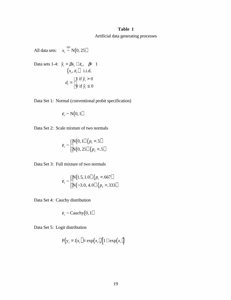
We used five data generating processes, shown in Table 1. In each process, there is a

single explanatory variable with mean zero and standard deviation five, and a coefficient of

one. The first three processes are special cases of the mixture of normals probit

specification. The first is a conventional probit model. The second and third are mixturesof two normals, the third having a bimodal distribution of the shock ε t . In the fourth data

generating process, the shock is Cauchy, and in the fifth, it is logit. The sample size is

2,000 in every process.

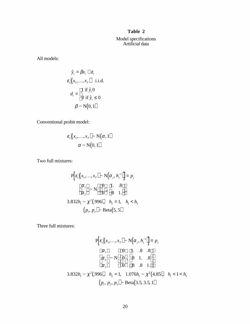
We used three model specifications, shown in Table 2. In each specification, the prior

distribution of the slope and intercept coefficients is independent standard normal. In the

specifications with two or more mixtures, the prior correlation of the intercept coefficients

is .8, which indicates that the coefficients are believed close together relative to their

distance from zero. The first model is the conventional probit model. The second model

has two mixtures: a labeling restriction on the precisions and a setting of the larger

precision to unity. The parameters of the prior distribution are chosen so that the upper 5%

of the distribution for h1 is truncated by the labeling restriction h1 < 1 and so that the .05

quantile is h1 =.01. Thus, this prior distribution allows considerable scope for a leptokurtic

distribution. The third model has three mixtures, again using a labeling restriction on the

precisions, with h2 = 1. The smaller precision has the same prior distribution as in the

9

preceding model. For the larger prior precision , the lower 5% of the distribution istruncated by the labeling restriction h3 > 1, and the .95 quantile is h3 = 10 .

We carried out computations on a Sun Ultra 200 Sparcstation using software written in

Fortran 77. In each computation 10,000 iterations of the Gibbs sampler were employed,

and the last 8,000 were used in the approximation of posterior moments. Computation

time was 14 minutes for the conventional probit model, 28 minutes for the mixture of two

normals, and 39 minutes for the mixture of three normals. Since the draws exhibit positive

serial correlation, there is less information in 8,000 iterations than there would be in 8,000

hypothetical i.i.d. drawings from the posterior distribution. The ratio of the number of

such i.i.d. draws to the number required in any given posterior simulator is the relative

numerical efficiency of that posterior simulator. In the conventional probit model relative

numerical efficiency for the Gibbs sampler was between .1 and .2 for most moments. In

the mixture of two normals, it was between .01 and 06. In the mixture of three normals, it

was between .005 and .05.

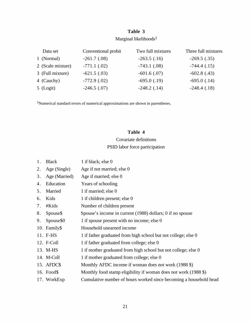
Discrimination between models using Bayes factors is of considerable interest. Table

3 shows marginal likelihoods for all data sets and models. Consider first the data generated

from the conventional probit model (set 1). The Bayes factor in favor of the conventional

probit model is 16 over the two-mixture model and 2,440 over the three-mixture model.

The intuitive interpretation of this result is that while the mixture models are correctly

specified, they spread prior probability over a larger space than does the conventional

probit model, which leaves less probability for the data generating process. This is an

example of how Bayes factors penalize excessive parameterization.

For the data generated from the two-mixture specification, the Bayes factor against the

incorrectly specified conventional probit model is overwhelming (about 1.45 ×1012 ). The

three-mixture model is correctly specified, but, again, the penalty for excessive

parameterization is exhibited in a Bayes factor of 3.7 in favor of the two-mixture model.

Results for the full-mixture data (set 3) are similar. For the case in which the distribution

of the disturbance is Cauchy, the Bayes factor between the two mixture models is one, but

the Bayes factor against the conventional probit specification is huge: 6.78 ×1033 . Neither

the two- nor the three-mixture model provides an improvement on the conventional probit

model in the case of the logistic distribution, with the Bayes factor in favor of the

conventional probit model being 5.5 against the two-mixture model and 6.7 against the

three-mixture model. In view of the well-documented great similarity of the probit and

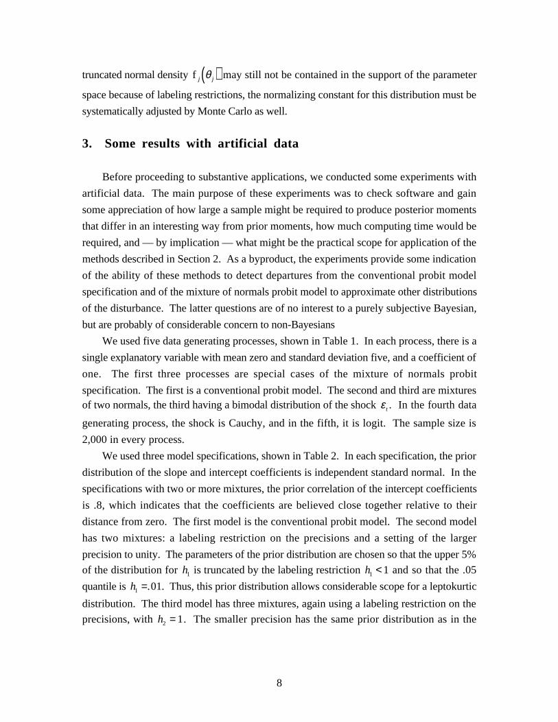
logit specifications (Maddala 1983), these findings for the logit data are not surprising.The predictive distributions, P d = 1 x( ) , are the main focus of interest in any

application of these models. Figures 1 through 5 show some aspects of these distributions

10

for the five data sets, respectively. Each figure corresponds to one of the artificial data

generating processes shown in Table 1, and each contains six panels. Each panel shows a

relevant range of x values on the horizontal axis. The three panels on the left indicate thevalue of P d = 1 x( ) in the data generating process with a solid line and the .25 and .75

posterior quantiles for this population value with dotted and dashed lines, respectively.The three panels on the right indicate the derivative of P d = 1 x( ) with respect to x in the

data generating process with a solid line, and .25 and .75 posterior quantiles for this

population value with dotted and dashed lines. The upper pair of panels shows results for

the conventional probit model, the middle pair for the two full mixture model, and the third

pair for the three full mixture model.

Results for the conventional probit data generating process are shown in Figure 1. For

a well-specified model and large sample sizes, we expect that the population value ofP d = 1 x( ) and its first derivative would be bracketed by the posterior .25 and .75 quantiles

about half the time. On the one hand, the conventional probit data generating process is a

special case of all three model probability density functions (p.d.f.’s), but the posteriorinterquartile values match the population P d = 1 x( ) better for the conventional probit

specification than for either of the mixture models. On the other hand, there are not many

values of x for which there is a serious discrepancy between posterior and data generating

process (DGP) in the sense that the true value lies more than an interquartile range’s width

from the boundary of the interquartile range itself. The obvious deterioration in the visual

match between distributions evident in Figure 1, in moving from the conventional probit to

the more complicated mixture of normals models, is reflected in the marginal likelihoods in

the first row of Table 3.

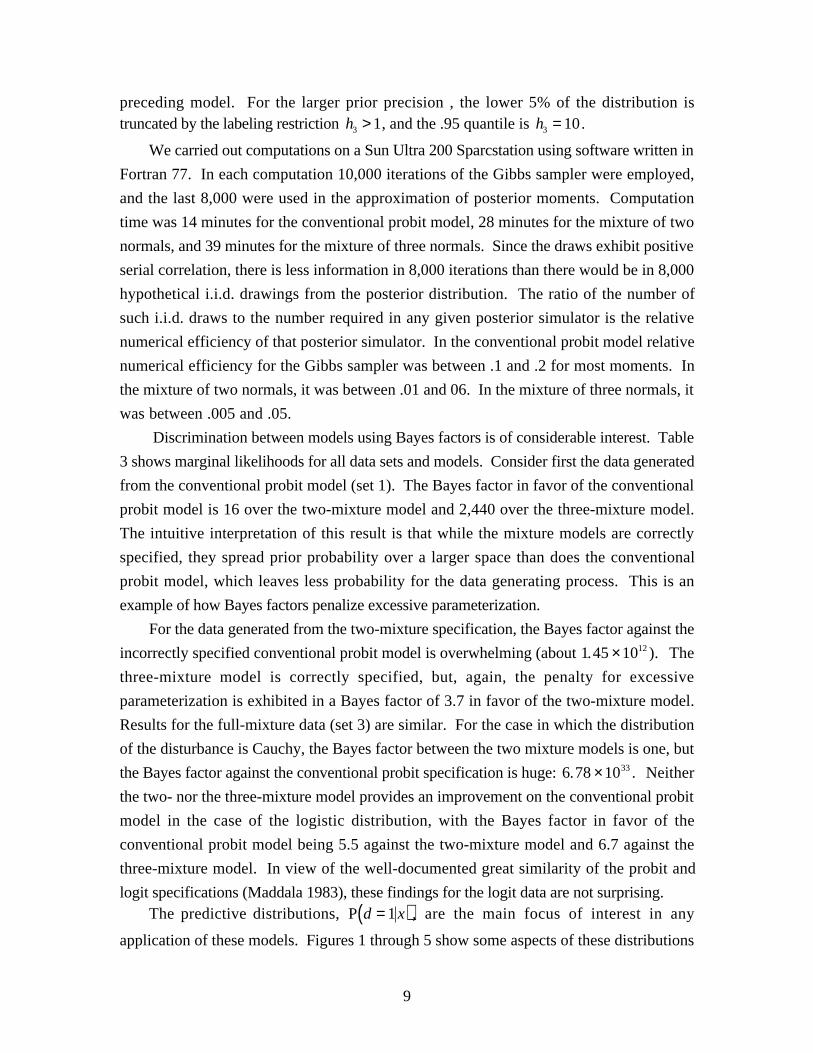
In the case of the scale mixture of normals data generating process (Figure 2), the

conventional probit model correctly specifies a symmetric distribution of the disturbance,

but cannot capture the thick tails of the population density. The most obvious feature of

Figure 2 is the distance of the posterior interquartile values from the population values ofP d = 1 x( ) for the conventional probit model and the corresponding closeness for the

mixture models. This is reflected in the marginal likelihood values in the second row of

Table 3. Interquartile ranges are larger for the two-mixture model than for the conventional

probit model and slightly larger yet for the three-mixture model. But the fit of the

conventional probit model is so bad that its probability is very low relative to the other two

(as indicated in the second row of Table 3). The three-mixture model looks a little closer to

the DGP than does the two-mixture model in the interquartile range metric, but the

interquartile range is sufficiently larger that it receives a little lower marginal likelihood.

11

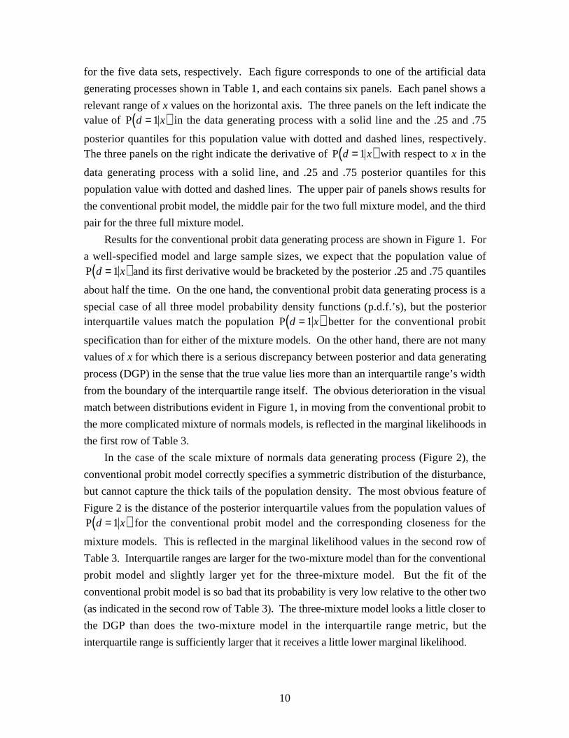
The full mixture of normals DGP implies a bimodal p.d.f. for the shock. None of the

models captures the bimodality, as indicated in Figure 3, but the mixture models come

much closer than does the conventional probit model. As was the case for the scale mixture

of normals DGP, interquartile ranges increase with model complexity. The conventional

model has difficulty with the tails, complicated by the asymmetry of the distribution.Although the population distribution of ε t has mean zero, its median is positive. The

distribution in the conventional probit specification is symmetric, and this causesoverprediction rather than underprediction of P d = 1 x( ) for small values of x. The mixture

models exhibit difficulties that are similar qualitatively but of considerably less importance

quantitatively. This behavior is due to the prior distribution of α , in which the standard

deviation of α1 − α2 is .63, whereas the population value of α1 − α2 is over seven times

this value. The prior is centered at a symmetric distribution, and so under- and over-

prediction similar to the conventional probit model results.

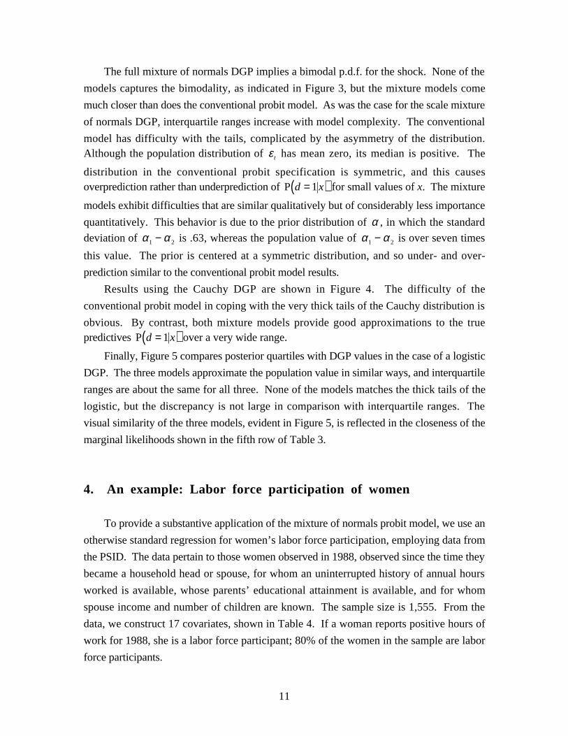
Results using the Cauchy DGP are shown in Figure 4. The difficulty of the

conventional probit model in coping with the very thick tails of the Cauchy distribution is

obvious. By contrast, both mixture models provide good approximations to the truepredictives P d = 1 x( ) over a very wide range.

Finally, Figure 5 compares posterior quartiles with DGP values in the case of a logistic

DGP. The three models approximate the population value in similar ways, and interquartile

ranges are about the same for all three. None of the models matches the thick tails of the

logistic, but the discrepancy is not large in comparison with interquartile ranges. The

visual similarity of the three models, evident in Figure 5, is reflected in the closeness of the

marginal likelihoods shown in the fifth row of Table 3.

4. An example: Labor force participation of women

To provide a substantive application of the mixture of normals probit model, we use an

otherwise standard regression for women’s labor force participation, employing data from

the PSID. The data pertain to those women observed in 1988, observed since the time they

became a household head or spouse, for whom an uninterrupted history of annual hours

worked is available, whose parents’ educational attainment is available, and for whom

spouse income and number of children are known. The sample size is 1,555. From the

data, we construct 17 covariates, shown in Table 4. If a woman reports positive hours of

work for 1988, she is a labor force participant; 80% of the women in the sample are labor

force participants.

12

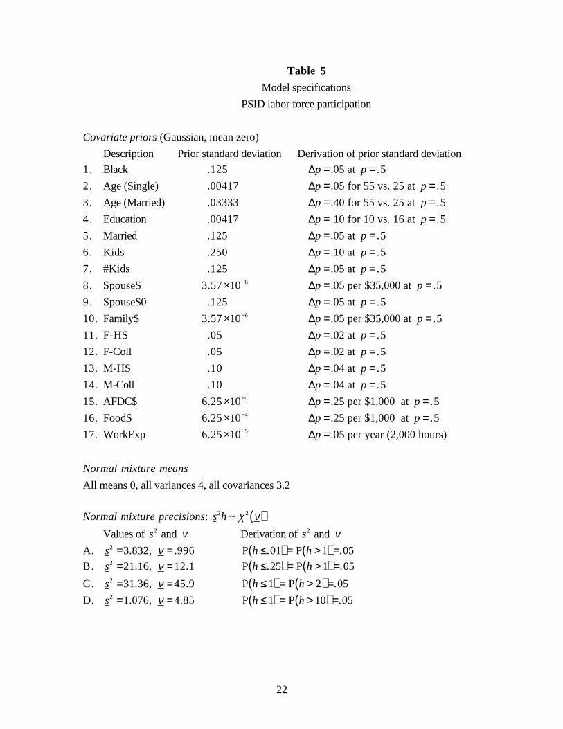
For the purposes of this illustration, independent Gaussian priors were constructed for

each of the 17 covariate coefficients. In each case, the prior distribution has mean zero.

The standard deviation is chosen by considering a large but reasonable effect of a change in

the corresponding covariate on the probability of labor force participation, given that the

probability of labor force participation is about one-half. This construction of the prior

distribution for β is shown in Table 5, which provides the prior standard deviation for

each coefficient along with the reasoning about effects on probability of labor force

participation that led to the choice.

The prior distribution for the mean vector α of the normal mixture is the same as that

used for the artificial data. The full specification of the normal mixture models is based on

combinations of four prior distributions for precisions, indicated at the bottom of Table 5.

Priors A and D were introduced in the experiments with artificial data. Prior B constrains

the precision to be less than one, but places much smaller probability on very low

precisions than does prior A. Prior C constrains the precision to be greater than one, but

places smaller probability on high precisions than does prior D.

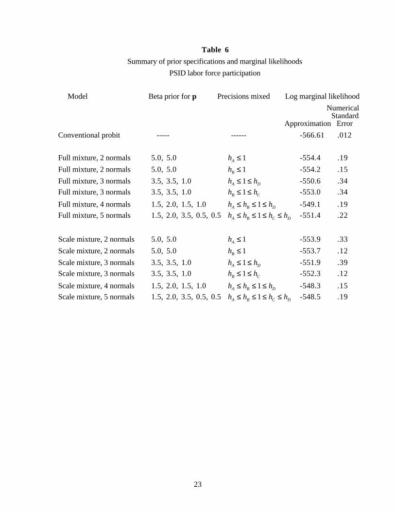
We report results for 13 models, shown in Table 6. Besides the conventional probit

models, there are two groups of mixture of normals probit models. The first group uses

scale mixtures of normals, thereby imposing symmetry of the shock distribution, and the

second group uses full mixtures of normals. The idea is to vary the number of mixtures by

using combinations of the prior distributions for precisions shown in Table 5 and labeling

restrictions on precisions to identify the mixtures. In the case of mixtures of two and three

normals, some alternative prior distributions are used to gauge the effect of alternative prior

distributions for the mixtures on marginal likelihood.

Formal model comparison is straightforward based on the marginal likelihoods shown

in Table 6. The most striking feature of the results is the poor performance of the

conventional probit model relative to the mixture of normals probit models. Relative to the

conventional probit model, the Bayes factor in favor of the mixture of normals model with

the smallest marginal likelihood (the full mixture of two normals employing hA ≤ 1) is

200,000. Relative to this latter model, the Bayes factor in favor of the mixture of normals

model with the largest marginal likelihood (the scale mixture of four normals) is 445. A

second regular feature of the results is that for both the full mixture and the scale mixture

groups, marginal likelihood increases as the number of mixtures is increased from two to

three to four and then decreases slightly for the mixture of five normals. The mixtures of

four and five normals provide an extremely rich family for a univariate distribution, with

anywhere from 6 (scale mixture of four normals) to 13 (full mixture of five normals)

parameters. Nevertheless, these models more than carry their own weight in the sense that

13

this increased uncertainty about the form of the distribution is more than compensated by

the better explanation of the data. A final regular feature of the results is evidence in favor

of scale mixture models as opposed to full mixture models. However, this evidence is not

strong. In some cases, the difference is on the order of numerical approximation error, and

in one case, the full mixture model is preferred.

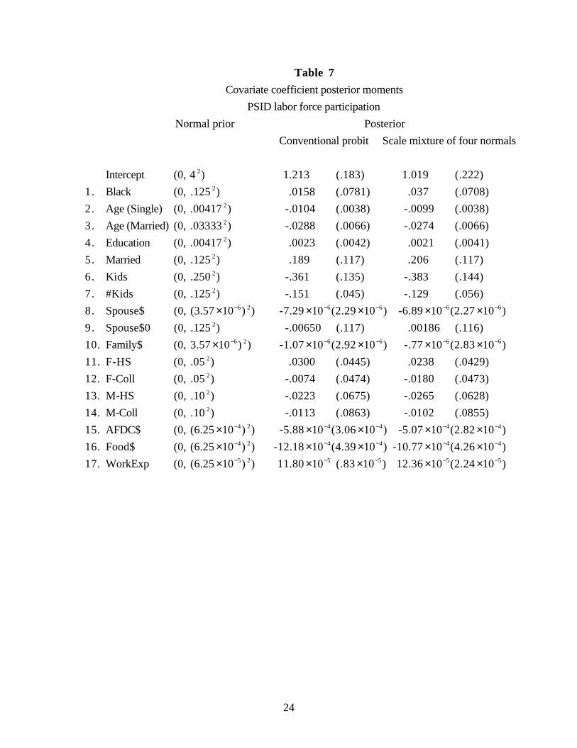
Posterior moments of the covariate coefficients in the conventional probit model, and

in the scale mixture of four normals model, are shown in Table 7. The coefficients in the

two models have different meanings, since the distributions of the shocks in the models are

not the same. Nevertheless, the posterior means and standard deviations are quite similar.

Seven of the seventeen covariates are important in the sense that their posterior means are

on the order of the large but reasonable effects used to choose the prior standard deviations.

(See Table 5.) These posterior means are also several posterior standard deviations from

zero in each case. Probability of labor force participation declines with age for both single

and married women. As expected, the effect is greater for married than single women,

which corresponds to a change in probability of about 12% over 30 years for married

women and 35% over 30 years for single women if labor force participation probabilities

are around 50%. Labor force participation probability declines by about 20% with the first

child and by about 6% for each child thereafter (again, beginning from participation

probabilities of around 50%). Spouse income, Aid to Families with Dependent Children

(AFDC), food stamp benefits, and cumulative work experience all have strong effects on

the probability of labor force participation. Further details on these effects are presented

below.

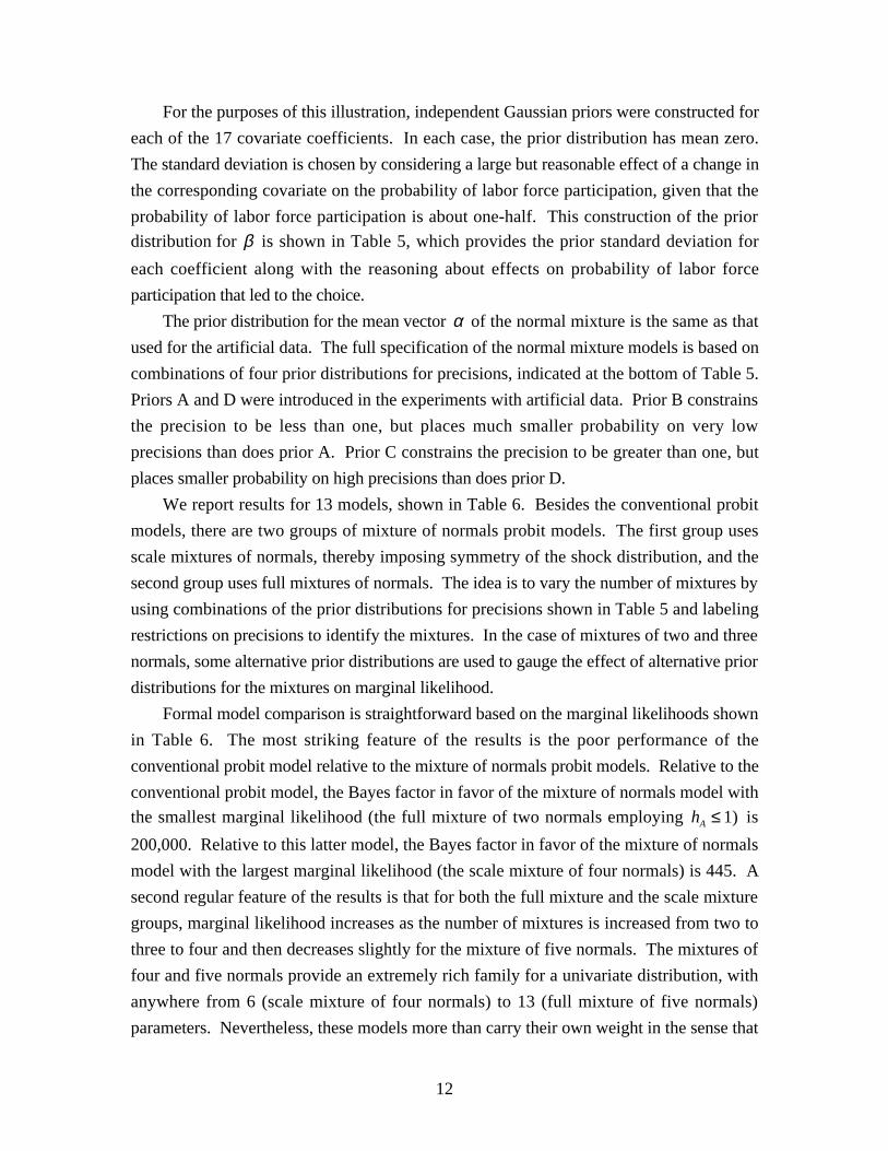
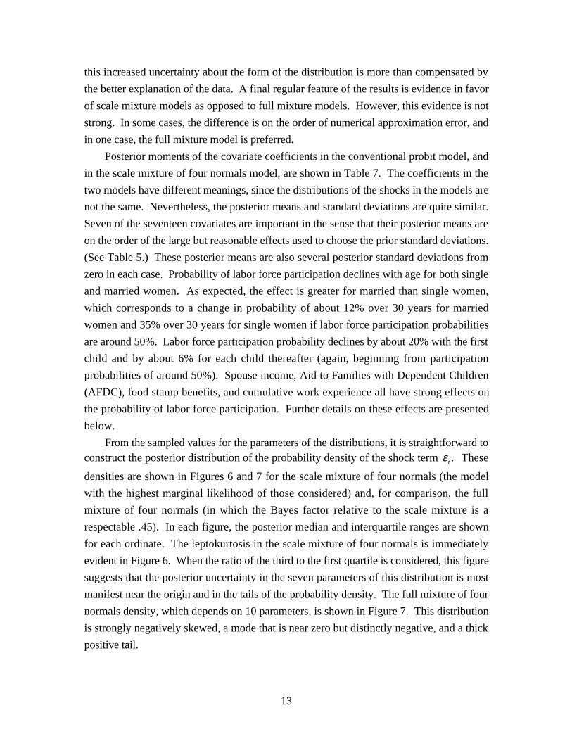
From the sampled values for the parameters of the distributions, it is straightforward toconstruct the posterior distribution of the probability density of the shock term ε t . These

densities are shown in Figures 6 and 7 for the scale mixture of four normals (the model

with the highest marginal likelihood of those considered) and, for comparison, the full

mixture of four normals (in which the Bayes factor relative to the scale mixture is a

respectable .45). In each figure, the posterior median and interquartile ranges are shown

for each ordinate. The leptokurtosis in the scale mixture of four normals is immediately

evident in Figure 6. When the ratio of the third to the first quartile is considered, this figure

suggests that the posterior uncertainty in the seven parameters of this distribution is most

manifest near the origin and in the tails of the probability density. The full mixture of four

normals density, which depends on 10 parameters, is shown in Figure 7. This distribution

is strongly negatively skewed, a mode that is near zero but distinctly negative, and a thick

positive tail.

14

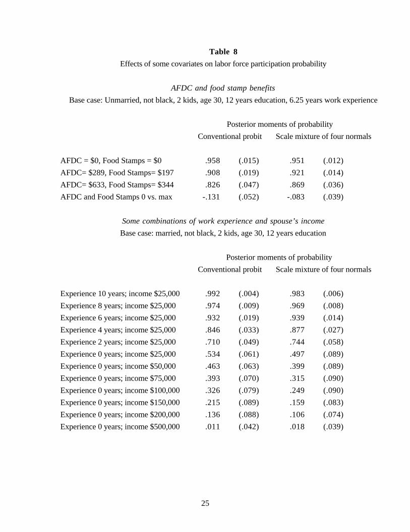
Some predictive distributions of interest are shown in Table 8. Two examples are

studied. In each example, results are shown for the conventional probit model and for the

mixture of normals probit model with the highest marginal likelihood. In the first example,

the probability of labor force participation for a 30-year-old woman with two children and

no spouse present is examined, as AFDC and food stamp benefit levels (given no labor

force participation) are changed from no benefits to the sample average for a woman in this

situation in 1988 to the sample maximum. In the conventional probit model, the increase of

benefits from zero to the maximum increases the probability of labor force nonparticipation

from .042 to .174, while in the scale mixture of four normals model, the increase is only

from .049 to .131. Notice that the posterior standard deviation of the labor force

participation probabilities is lower in the scale mixture model than in the conventional probit

model in every case: uncertainty about the individual parameters in this model, taken in

isolation, does not imply greater uncertainty about the predictive probabilities than in the

case of the conventional probit model where there is no uncertainty about the shape of the

shock distribution.

In the second example shown in Table 8, cumulative labor market experience and

spouse’s income are varied for a married woman aged 30 with two children so as to vary

the probability of labor force participation between roughly .01 and .99. Differences in the

posterior means of participation probabilities can be appreciable, reaching .078 (about one

posterior standard deviation) for a woman with no labor market experience and a spouse

earning $75,000 per year. Ratios for participation or nonparticipation approach two when

these probabilities are small. When probabilities of both participation and non-participation

are substantial, the posterior standard deviations in the conventional probit model tend to be

smaller, whereas when one is small and one is large, there is less uncertainty in the scale

mixture of normals model.

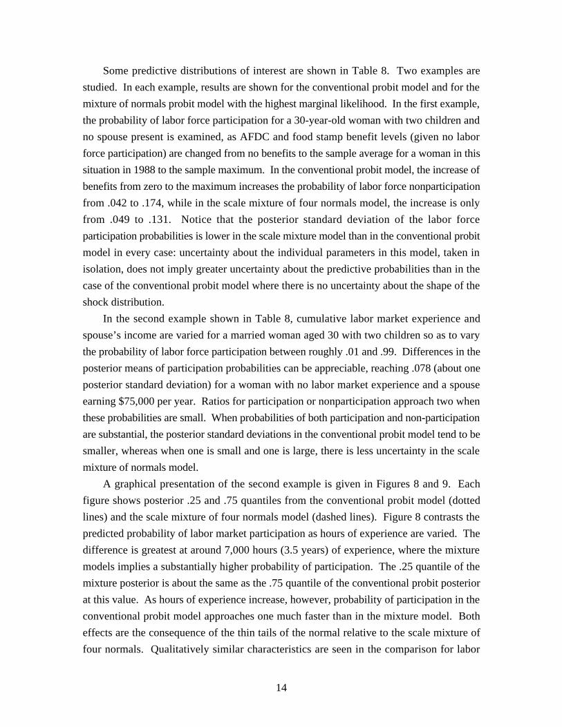
A graphical presentation of the second example is given in Figures 8 and 9. Each

figure shows posterior .25 and .75 quantiles from the conventional probit model (dotted

lines) and the scale mixture of four normals model (dashed lines). Figure 8 contrasts the

predicted probability of labor market participation as hours of experience are varied. The

difference is greatest at around 7,000 hours (3.5 years) of experience, where the mixture

models implies a substantially higher probability of participation. The .25 quantile of the

mixture posterior is about the same as the .75 quantile of the conventional probit posterior

at this value. As hours of experience increase, however, probability of participation in the

conventional probit model approaches one much faster than in the mixture model. Both

effects are the consequence of the thin tails of the normal relative to the scale mixture of

four normals. Qualitatively similar characteristics are seen in the comparison for labor

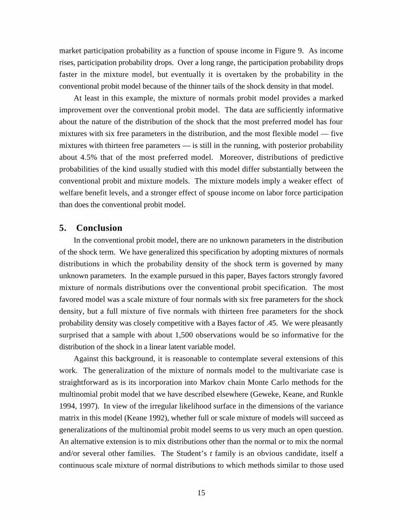
15

market participation probability as a function of spouse income in Figure 9. As income

rises, participation probability drops. Over a long range, the participation probability drops

faster in the mixture model, but eventually it is overtaken by the probability in the

conventional probit model because of the thinner tails of the shock density in that model.

At least in this example, the mixture of normals probit model provides a marked

improvement over the conventional probit model. The data are sufficiently informative

about the nature of the distribution of the shock that the most preferred model has four

mixtures with six free parameters in the distribution, and the most flexible model — five

mixtures with thirteen free parameters — is still in the running, with posterior probability

about 4.5% that of the most preferred model. Moreover, distributions of predictive

probabilities of the kind usually studied with this model differ substantially between the

conventional probit and mixture models. The mixture models imply a weaker effect of

welfare benefit levels, and a stronger effect of spouse income on labor force participation

than does the conventional probit model.

5. ConclusionIn the conventional probit model, there are no unknown parameters in the distribution

of the shock term. We have generalized this specification by adopting mixtures of normals

distributions in which the probability density of the shock term is governed by many

unknown parameters. In the example pursued in this paper, Bayes factors strongly favored

mixture of normals distributions over the conventional probit specification. The most

favored model was a scale mixture of four normals with six free parameters for the shock

density, but a full mixture of five normals with thirteen free parameters for the shock

probability density was closely competitive with a Bayes factor of .45. We were pleasantly

surprised that a sample with about 1,500 observations would be so informative for the

distribution of the shock in a linear latent variable model.

Against this background, it is reasonable to contemplate several extensions of this

work. The generalization of the mixture of normals model to the multivariate case is

straightforward as is its incorporation into Markov chain Monte Carlo methods for the

multinomial probit model that we have described elsewhere (Geweke, Keane, and Runkle

1994, 1997). In view of the irregular likelihood surface in the dimensions of the variance

matrix in this model (Keane 1992), whether full or scale mixture of models will succeed as

generalizations of the multinomial probit model seems to us very much an open question.

An alternative extension is to mix distributions other than the normal or to mix the normal

and/or several other families. The Student’s t family is an obvious candidate, itself a

continuous scale mixture of normal distributions to which methods similar to those used

16

here can be applied (Geweke 1993). Finally, we note that the assumption of linearity in thecovariates x t is as much a convenient assumption, in most applications, as is normalilty in

the conventional probit model. Relaxing this assumption in favor of the obvious expansion

families (for example, Taylor or Laurent series) is straightforward and lends itself well to

incorporation of subjective priors in the way we have done here. Clearly, there are

interactions between relaxing both linearity and normality; in the limit, one cannot do both.

We plan to explore these issues in future work.

17

References

Albert, J.H. and S. Chib, 1993, “Bayesian Analysis of Binary and PolychotomousResponse Data,” Journal of the American Statistical Association 88: 669–679.

Aldrich, J., and F. Nelson, 1984, Linear Probability, Logit, and Probit Models.Beverly Hills: Sage Publications.

Cosslett, S.R., 1983, “Distribution-Free Maximum Likelihood Estimator of the BinaryChoice Model,” Econometrica 51: 765–782.

Gallant, A.R., and D.W. Nychka, 1987, “Semi-Nonparametric Maximum LikelihoodEstimation,” Econometrica 55: 363–390.

Gelfand, A.E., and D.K. Dey, 1994, “Bayesian Model Choice: Asymptotics and ExactCalculations,” Journal of the Royal Statistical Society Series B 56: 501–514.

Geweke, J., 1991, “Efficient Simulation from the Multivariate Normal and Student-tDistributions Subject to Linear Constraints,” in E. M. Keramidas (ed.), ComputingScience and Statistics: Proceedings of the Twenty-Third Symposium on theInterface, 571–578. Fairfax: Interface Foundation of North America, Inc.

Geweke, J., 1993, “Bayesian Treatment of the Independent Student-t Linear Model,”Journal of Applied Econometrics 8: S19–S40.

Geweke, J., 1997a, “Posterior Simulators in Econometrics,” in D. Kreps and K.F Wallis(eds.), Advances in Economics and Econometrics: Theory and Applications, vol.III, 128–165. Cambridge: Cambridge University Press.

Geweke, J., 1997b, “Simulation-Based Bayesian Inference for Economic Time Series,” inR.S. Mariano, T. Schuermann and M. Weeks (eds.), Simulation-Based Inference inEconometrics: Methods and Applications. Cambridge: Cambridge UniversityPress, forthcoming.

Geweke, J., M. Keane, and D. Runkle, 1994, “Alternative Computational Approaches toInference in the Multinomial Probit Model,” Review of Economics and Statistics,76: 609–632.

Geweke, J., M. Keane, and D. Runkle, 1997, “Statistical Inference in the MultinomialMultiperiod Probit Model,” Journal of Econometrics 80: 125-166.

Hausman, J., and D. McFadden, 1984, “Specification Tests for the Multinomial LogitModel,” Econometrica 52: 1219–1240.

Horowitz, J.L., 1992, “A Smoothed Maximum Score Estimator for the Binary ResponseModel,” Econometrica 60: 505–531.

Ichimura, H., 1993, “Semiparametric Least Squares (SLS) and Weighted SLS Estimationof Single-Index Models,” Journal of Econometrics 58: 71–120.

Keane, M.P., 1992, “A Note on Identification in the Multinomial Probit Model,” Journalof Business and Economic Statistics 10: 193–200.

18

Klein, R.W. and R.H. Spady, 1993, “An Efficient Semiparametric Estimator for BinaryResponse Models,” Econometrica 61: 387–421.

Koop, G., and D. J. Poirier, 1993, “Bayesian Analysis of Logit Models Using NaturalConjugate Priors,” Journal of Econometrics 56: 323–340.

Lewbel, A., 1997, “Semiparametric Estimation of Location and Other Discrete ChoiceMoments,” Econometric Theory 13: 32–51.

Maddala, G.S., 1983, Limited Dependent and Qualitative Variables in Econometrics.Cambridge: Cambridge University Press.

Manski, C.F., 1985, “Semiparametric Analysis of Discrete Response: AsymptoticProperties of the Maximum Score Estimator,” Journal of Econometrics 27: 313–333.

Powell, J.L., J.H. Stock, and T.M. Stoker, 1989, “Semiparametric Estimation of IndexCoefficients,” Econometrica 57: 1403–1430.

Roberts, G.O., and A.F.M. Smith, 1994, “Simple Conditions for the Convergence of theGibbs Sampler and Metropolis-Hastings Algorithms,” Stochastic Processes andTheir Applications 49: 207–216.

Tierney, L., 1994, “Markov Chains for Exploring Posterior Distributions” (withdiscussion and rejoinder), Annals of Statistics 22: 1701–1762.

Zellner, A., and P.E. Rossi, 1984, “Bayesian Analysis of Dichotomous Quantal ResponseModels,” Journal of Econometrics 25: 365–393.

19

Table 1

Artificial data generating processes

All data sets: xt ~IID

N 0, 25( )

Data sets 1-4: ˜ ,y xt t t= + =β ε β 1

x

dy

y

t t

t

t

t

,

˜

˜

ε( )

=>≤

i.i.d.

if

if

1 0

0 0

Data Set 1: Normal (conventional probit specification)

ε t ~ N 0, 1( )

Data Set 2: Scale mixture of two normals

ε t ~N 0, 1( ) p1 =.5( )N 0, 25( ) p2 =.5( )

Data Set 3: Full mixture of two normals

ε t ~N 1.5, 1.0( ) p1 =.667( )N −3.0, 4.0( ) p2 =.333( )

Data Set 4: Cauchy distribution

ε t ~ Cauchy 0, 1( )

Data Set 5: Logit distribution

P yt = 1 xt( ) = exp xt( ) 1 + exp xt( )[ ]

20

Table 2

Model specificationsArtificial data

All models:

˜

, ,

˜

˜

~ N ,

y x

x x

dy

y

t t t

t T

t

t

t

= +

( )

=≤

( )

β ε

ε

β

1

1 0

0 0

0 1

K i.i.d.

if

if

Conventional probit model:

ε t x1,K, xT( ) ~ N α, 1( )α ~ N 0, 1( )

Two full mixtures:

P , , ~ N ,

~ N ,. .

. .

. ~ . , ,

, ~ Beta ,

ε α

αα

χ

t T j j jx x h p

h h h h

p p

11

1

2

12

2 1 2

1 2

0

0

1 8

8 1

3 832 996 1

5 5

K( ) ( )[ ] =

( ) = <

( ) ( )

−

Three full mixtures:

P , , ~ N ,

~ N ,

. . .

. . .

. . .

. ~ . , , . ~

ε α

ααα

χ χ

t T j j jx x h p

h h h

11

1

2

3

12

2 3

0

0

0

1 8 8

8 1 8

8 8 1

3 832 996 1 1 076

K( ) ( )[ ] =

( ) =

−

221 3

1 2 3

4 85 1

3 5 3 5 1

. ;

, , ~ Beta . , . ,

( ) < <

( ) ( )h h

p p p

21

Table 3

Marginal likelihoods1

Data set Conventional probit Two full mixtures Three full mixtures

1 (Normal) -261.7 (.08) -263.5 (.16) -269.5 (.35)

2 (Scale mixture) -771.1 (.02) -743.1 (.08) -744.4 (.15)

3 (Full mixture) -621.5 (.03) -601.6 (.07) -602.8 (.43)

4 (Cauchy) -772.9 (.02) -695.0 (.19) -695.0 (.14)

5 (Logit) -246.5 (.07) -248.2 (.14) -248.4 (.18)

1Numerical standard errors of numerical approximations are shown in parentheses.

Table 4

Covariate definitions

PSID labor force participation

1. Black 1 if black; else 0

2. Age (Single) Age if not married; else 0

3. Age (Married) Age if married; else 0

4. Education Years of schooling

5. Married 1 if married; else 0

6. Kids 1 if children present; else 0

7. #Kids Number of children present

8. Spouse$ Spouse’s income in current (1988) dollars; 0 if no spouse

9. Spouse$0 1 if spouse present with no income; else 0

10. Family$ Household unearned income

11. F-HS 1 if father graduated from high school but not college; else 0

12. F-Coll 1 if father graduated from college; else 0

13. M-HS 1 if mother graduated from high school but not college; else 0

14. M-Coll 1 if mother graduated from college; else 0

15. AFDC$ Monthly AFDC income if woman does not work (1988 $)

16. Food$ Monthly food stamp eligibility if woman does not work (1988 $)

17. WorkExp Cumulative number of hours worked since becoming a household head

22

Table 5

Model specifications


Covariate priors (Gaussian, mean zero)

Description Prior standard deviation Derivation of prior standard deviation

1. Black .125 ∆p = .05 at p = .5

2. Age (Single) .00417 ∆p = .05 for 55 vs. 25 at p = .5

3. Age (Married) .03333 ∆p = .40 for 55 vs. 25 at p = .5

4. Education .00417 ∆p = .10 for 10 vs. 16 at p = .5

5. Married .125 ∆p = .05 at p = .5

6. Kids .250 ∆p = .10 at p = .5

7. #Kids .125 ∆p = .05 at p = .5

8. Spouse$ 3.57 ×10−6 ∆p = .05 per $35,000 at p = .5

9. Spouse$0 .125 ∆p = .05 at p = .5

10. Family$ 3.57 ×10−6 ∆p = .05 per $35,000 at p = .5

11. F-HS .05 ∆p = .02 at p = .5

12. F-Coll .05 ∆p = .02 at p = .5

13. M-HS .10 ∆p = .04 at p = .5

14. M-Coll .10 ∆p = .04 at p = .5

15. AFDC$ 6.25 ×10−4 ∆p = .25 per $1,000 at p = .5

16. Food$ 6.25 ×10−4 ∆p = .25 per $1,000 at p = .5

17. WorkExp 6.25 ×10−5 ∆p = .05 per year (2,000 hours)

Normal mixture means

All means 0, all variances 4, all covariances 3.2

Normal mixture precisions: s2h ~ χ 2 ν( )Values of s2 and ν Derivation of s2 and ν

A. s2 =3.832, ν = .996 P h ≤.01( ) = P h > 1( ) =.05

B. s2 =21.16, ν =12.1 P h ≤.25( ) = P h > 1( ) =.05

C. s2 =31.36, ν =45.9 P h ≤ 1( ) = P h > 2( ) =.05

D. s2 =1.076, ν =4.85 P h ≤ 1( ) = P h > 10( ) =.05

23

Table 6

Summary of prior specifications and marginal likelihoods


Model Beta prior for p Precisions mixed Log marginal likelihood

Numerical Standard

Approximation Error

Conventional probit ----- ------ -566.61 .012

Full mixture, 2 normals 5.0, 5.0 hA ≤ 1 -554.4 .19

Full mixture, 2 normals 5.0, 5.0 hB ≤ 1 -554.2 .15

Full mixture, 3 normals 3.5, 3.5, 1.0 hA ≤ 1 ≤ hD -550.6 .34

Full mixture, 3 normals 3.5, 3.5, 1.0 hB ≤ 1 ≤ hC -553.0 .34

Full mixture, 4 normals 1.5, 2.0, 1.5, 1.0 hA ≤ hB ≤ 1 ≤ hD -549.1 .19

Full mixture, 5 normals 1.5, 2.0, 3.5, 0.5, 0.5 hA ≤ hB ≤ 1 ≤ hC ≤ hD -551.4 .22

Scale mixture, 2 normals 5.0, 5.0 hA ≤ 1 -553.9 .33

Scale mixture, 2 normals 5.0, 5.0 hB ≤ 1 -553.7 .12

Scale mixture, 3 normals 3.5, 3.5, 1.0 hA ≤ 1 ≤ hD -551.9 .39

Scale mixture, 3 normals 3.5, 3.5, 1.0 hB ≤ 1 ≤ hC -552.3 .12

Scale mixture, 4 normals 1.5, 2.0, 1.5, 1.0 hA ≤ hB ≤ 1 ≤ hD -548.3 .15

Scale mixture, 5 normals 1.5, 2.0, 3.5, 0.5, 0.5 hA ≤ hB ≤ 1 ≤ hC ≤ hD -548.5 .19

24

Table 7

Covariate coefficient posterior moments


Normal prior Posterior

Conventional probit Scale mixture of four normals

Intercept (0, 4 2) 1.213 (.183) 1.019 (.222)

1. Black (0, .125 2) .0158 (.0781) .037 (.0708)

2. Age (Single) (0, .00417 2) -.0104 (.0038) -.0099 (.0038)

3. Age (Married) (0, .03333 2) -.0288 (.0066) -.0274 (.0066)

4. Education (0, .00417 2) .0023 (.0042) .0021 (.0041)

5. Married (0, .125 2) .189 (.117) .206 (.117)

6. Kids (0, .250 2) -.361 (.135) -.383 (.144)

7. #Kids (0, .125 2) -.151 (.045) -.129 (.056)

8. Spouse$ (0, (3.57 ×10−6) 2) -7.29 ×10−6(2.29 ×10−6) -6.89 ×10−6(2.27 ×10−6)

9. Spouse$0 (0, .125 2) -.00650 (.117) .00186 (.116)

10. Family$ (0, 3.57 ×10−6) 2) -1.07 ×10−6(2.92 ×10−6) -.77 ×10−6(2.83 ×10−6)

11. F-HS (0, .05 2) .0300 (.0445) .0238 (.0429)

12. F-Coll (0, .05 2) -.0074 (.0474) -.0180 (.0473)

13. M-HS (0, .10 2) -.0223 (.0675) -.0265 (.0628)

14. M-Coll (0, .10 2) -.0113 (.0863) -.0102 (.0855)

15. AFDC$ (0, (6.25 ×10−4) 2) -5.88 ×10−4(3.06 ×10−4) -5.07 ×10−4(2.82 ×10−4)

16. Food$ (0, (6.25 ×10−4) 2) -12.18 ×10−4(4.39 ×10−4) -10.77 ×10−4(4.26 ×10−4)

17. WorkExp (0, (6.25 ×10−5) 2) 11.80 ×10−5 (.83 ×10−5) 12.36 ×10−5(2.24 ×10−5)

25

Table 8

Effects of some covariates on labor force participation probability

AFDC and food stamp benefits

Base case: Unmarried, not black, 2 kids, age 30, 12 years education, 6.25 years work experience

Posterior moments of probability


AFDC = $0, Food Stamps = $0 .958 (.015) .951 (.012)

AFDC= $289, Food Stamps= $197 .908 (.019) .921 (.014)

AFDC= $633, Food Stamps= $344 .826 (.047) .869 (.036)

AFDC and Food Stamps 0 vs. max -.131 (.052) -.083 (.039)

Some combinations of work experience and spouse’s income

Base case: married, not black, 2 kids, age 30, 12 years education

Posterior moments of probability


Experience 10 years; income $25,000 .992 (.004) .983 (.006)












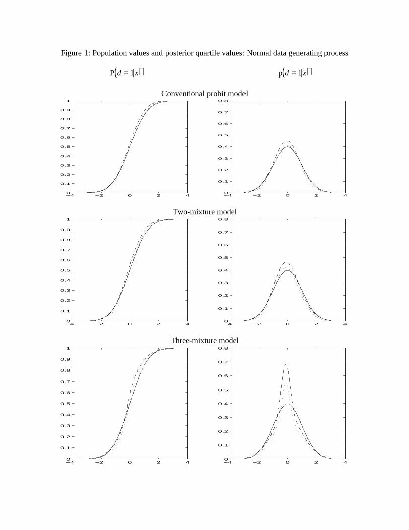
Figure 1: Population values and posterior quartile values: Normal data generating process

( )P d x= 1 ( )p d x= 1

Conventional probit model

−4 −2 0 2 40

0.1

0.2

0.3

0.4

0.5

0.6

0.7

0.8

0.9

1

−4 −2 0 2 40

0.1

0.2

0.3

0.4

0.5

0.6

0.7

0.8

Two-mixture model

−4 −2 0 2 40

0.1

0.2

0.3

0.4

0.5

0.6

0.7

0.8

0.9

1

−4 −2 0 2 40

0.1

0.2

0.3

0.4

0.5

0.6

0.7

0.8

Three-mixture model

−4 −2 0 2 40

0.1

0.2

0.3

0.4

0.5

0.6

0.7

0.8

0.9

1

−4 −2 0 2 40

0.1

0.2

0.3

0.4

0.5

0.6

0.7

0.8

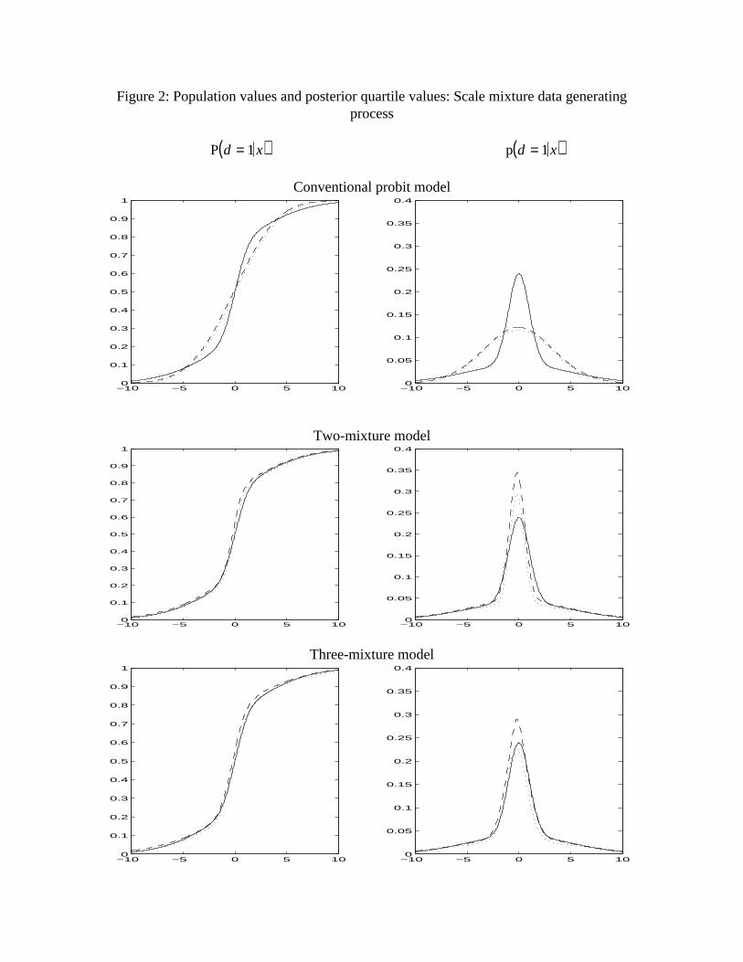
Figure 2: Population values and posterior quartile values: Scale mixture data generatingprocess

( )P d x= 1 ( )p d x= 1


−10 −5 0 5 100

0.05

0.1

0.15

0.2

0.25

0.3

0.35

0.4

−10 −5 0 5 100

0.1

0.2

0.3

0.4

0.5

0.6

0.7

0.8

0.9

1

Two-mixture model

−10 −5 0 5 100

0.05

0.1

0.15

0.2

0.25

0.3

0.35

0.4

−10 −5 0 5 100

0.1

0.2

0.3

0.4

0.5

0.6

0.7

0.8

0.9

1

Three-mixture model

−10 −5 0 5 100

0.05

0.1

0.15

0.2

0.25

0.3

0.35

0.4

−10 −5 0 5 100

0.1

0.2

0.3

0.4

0.5

0.6

0.7

0.8

0.9

1

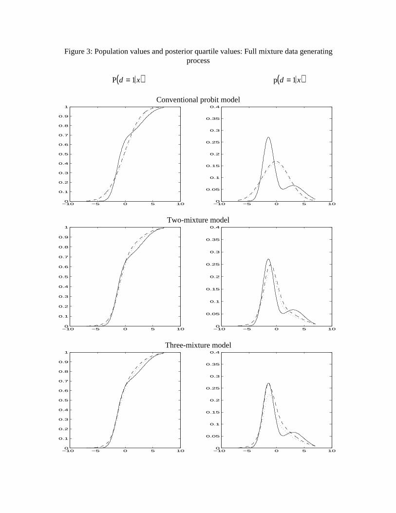
Figure 3: Population values and posterior quartile values: Full mixture data generatingprocess

( )P d x= 1 ( )p d x= 1


−10 −5 0 5 100

0.05

0.1

0.15

0.2

0.25

0.3

0.35

0.4

−10 −5 0 5 100

0.1

0.2

0.3

0.4

0.5

0.6

0.7

0.8

0.9

1

Two-mixture model

−10 −5 0 5 100

0.05

0.1

0.15

0.2

0.25

0.3

0.35

0.4

−10 −5 0 5 100

0.1

0.2

0.3

0.4

0.5

0.6

0.7

0.8

0.9

1

Three-mixture model

−10 −5 0 5 100

0.05

0.1

0.15

0.2

0.25

0.3

0.35

0.4

−10 −5 0 5 100

0.1

0.2

0.3

0.4

0.5

0.6

0.7

0.8

0.9

1

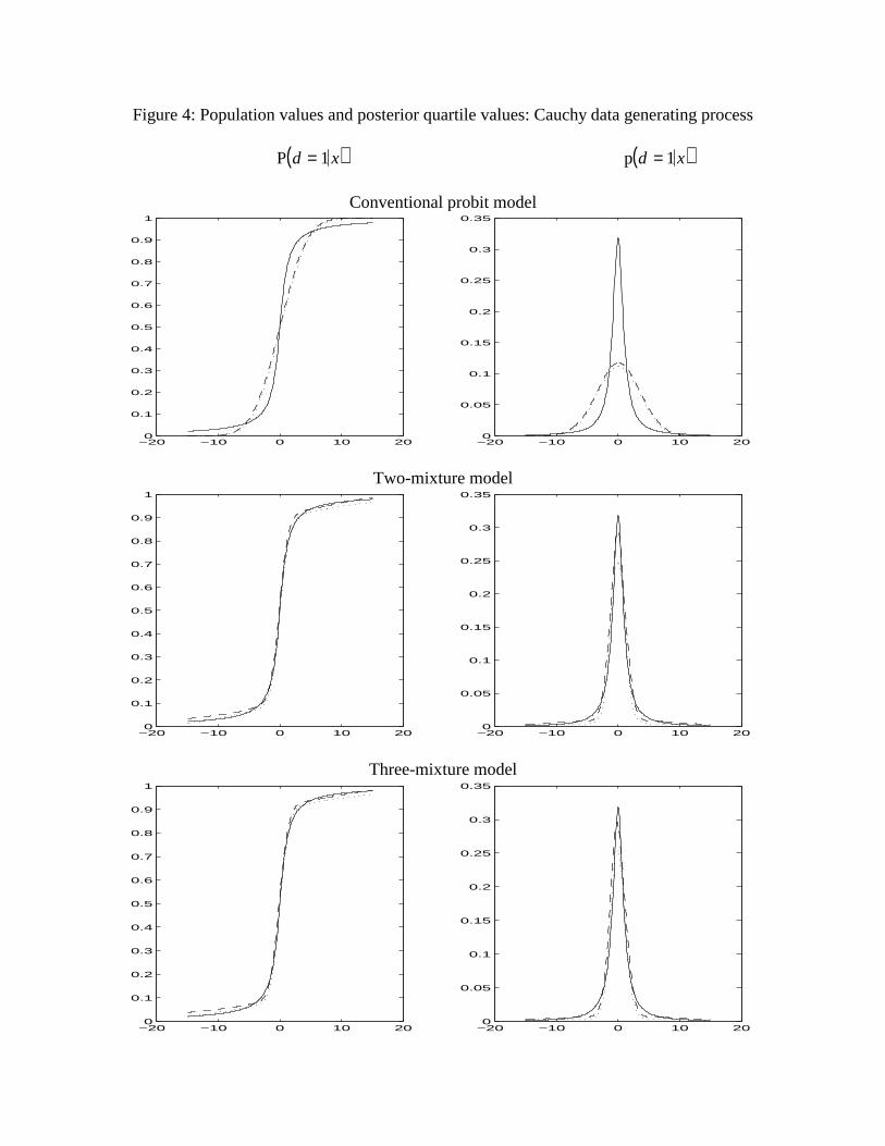
Figure 4: Population values and posterior quartile values: Cauchy data generating process

( )P d x= 1 ( )p d x= 1


−20 −10 0 10 200

0.05

0.1

0.15

0.2

0.25

0.3

0.35

−20 −10 0 10 200

0.1

0.2

0.3

0.4

0.5

0.6

0.7

0.8

0.9

1

Two-mixture model

−20 −10 0 10 200

0.05

0.1

0.15

0.2

0.25

0.3

0.35

−20 −10 0 10 200

0.1

0.2

0.3

0.4

0.5

0.6

0.7

0.8

0.9

1

Three-mixture model

−20 −10 0 10 200

0.05

0.1

0.15

0.2

0.25

0.3

0.35

−20 −10 0 10 200

0.1

0.2

0.3

0.4

0.5

0.6

0.7

0.8

0.9

1

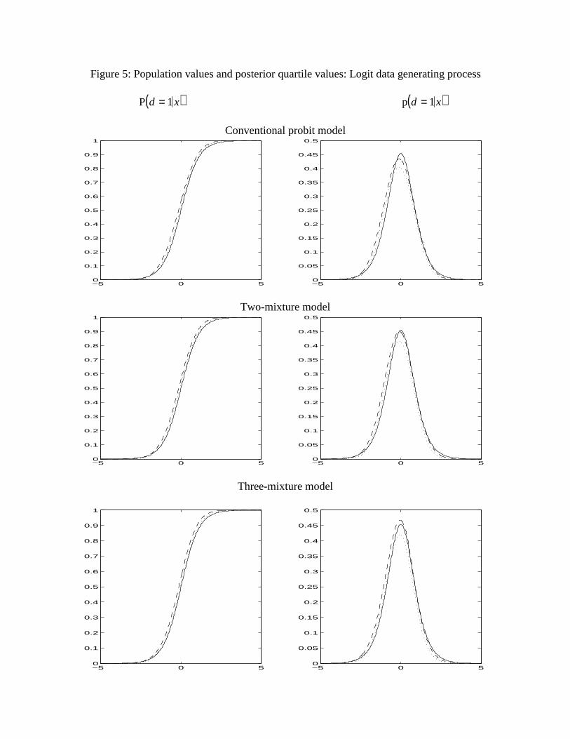
Figure 5: Population values and posterior quartile values: Logit data generating process

( )P d x= 1 ( )p d x= 1


−5 0 50

0.05

0.1

0.15

0.2

0.25

0.3

0.35

0.4

0.45

0.5

−5 0 50

0.1

0.2

0.3

0.4

0.5

0.6

0.7

0.8

0.9

1

Two-mixture model

−5 0 50

0.05

0.1

0.15

0.2

0.25

0.3

0.35

0.4

0.45

0.5

−5 0 50

0.1

0.2

0.3

0.4

0.5

0.6

0.7

0.8

0.9

1

Three-mixture model

−5 0 50

0.05

0.1

0.15

0.2

0.25

0.3

0.35

0.4

0.45

0.5

−5 0 50

0.1

0.2

0.3

0.4

0.5

0.6

0.7

0.8

0.9

1

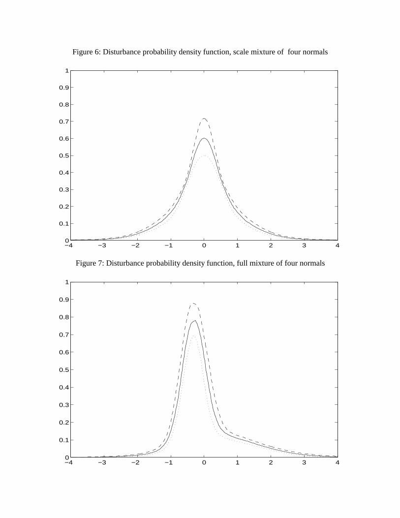
Figure 6: Disturbance probability density function, scale mixture of four normals

−4 −3 −2 −1 0 1 2 3 40

0.1

0.2

0.3

0.4

0.5

0.6

0.7

0.8

0.9

1

Figure 7: Disturbance probability density function, full mixture of four normals

−4 −3 −2 −1 0 1 2 3 40

0.1

0.2

0.3

0.4

0.5

0.6

0.7

0.8

0.9

1

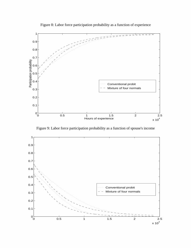
Figure 8: Labor force participation probability as a function of experience

Conventional probit

Mixture of four normals

0 0.5 1 1.5 2 2.5

x 104

0

0.1

0.2

0.3

0.4

0.5

0.6

0.7

0.8

0.9

1

Hours of experience

Parti

cipa

tion

prob

abilit

y

Figure 9: Labor force participation probability as a function of spouse's income

Conventional probit

Mixture of four normals

0 0.5 1 1.5 2 2.5

x 104

0

0.1

0.2

0.3

0.4

0.5

0.6

0.7

0.8

0.9

1

sr237 mixture of normals probit models - federal … · favor mixture of normals probit models over...

Documents