öMmföäflsäafaäsflassflassflasffffffffffffffffffffffffffffffffffff

Discussion Papers

Dynamic Probit Models and Financial Variablesin Recession Forecasting

Henri NybergUniversity of Helsinki and HECER

Discussion Paper No. 225June 2008

ISSN 1795-0562

HECER – Helsinki Center of Economic Research, P.O. Box 17 (Arkadiankatu 7), FI-00014University of Helsinki, FINLAND, Tel +358-9-191-28780, Fax +358-9-191-28781,E-mail info-hecer@helsinki.fi, Internet www.hecer.fi

HECERDiscussion Paper No. 225

Dynamic Probit Models and Financial Variablesin Recession Forecasting*

Abstract

In this paper various financial variables are examined as predictors in new dynamic probitmodels to predict the probability of a recession in the United States and Germany.Following the findings of previous studies, the domestic term spread proved to be animportant predictive variable, but several lagged values of stock returns and the foreignterm spread are also statistically significant predictive variables for both countries. Theinterest rate differential between the U.S. and Germany is also a useful predictor in thecase of Germany. Examined dynamic probit models outperform the traditional static modelgiving accurate out-of-sample forecasts for the latest recession period that began in bothcountries in 2001.

JEL Classification: C22, C25, E32, E37

Keywords: Dynamic probit models, recession forecast, term spread, stock return

Henri Nyberg

Department of EconomicsUniversity of HelsinkiP.O. Box 17 (Arkadiankatu 7)FI-00014 University of HelsinkiFINLAND

e-mail: henri.nyberg@helsinki.fi

* The author would like to thank Heikki Kauppi, Markku Lanne and Pentti Saikkonen forconstructive comments. The author is responsible for remaining errors. Financial supportfrom the Research Foundation of the University of Helsinki, Academy of Finland, theOkobank Group Research Foundation and the Finnish Foundation for Advancement ofSecurities Markets is gratefully acknowledged.

1 Introduction

A substantial amount of research has considered the predictive ability of various fi-

nancial variables to predict the economic growth and recession periods in different

countries. Much of the previous analysis is focused on time series models, where the

dependent variable is ”continuous” such as the growth rate of GDP and industrial

production. In the econometric literature, however, forecasting the values of the bi-

nary recession indicator with probit or logit models has attracted attention in recent

years when some new time series models for binary dependent variables have been

suggested. For instance, Rydberg and Shephard (2003), Chauvet and Potter (2005)

and Dueker (2005) proposed new dynamic extensions to the traditional static model

where the response probability is only a function of the explanatory variables.

Particularly, the term spread which is the difference between the long- and short-

term interest rate, is suggested in the literature to be a useful predictor of future

economic growth and recession periods (e.g. Estrella and Mishkin, 1998 and Estrella,

2005a). However, other financial variables have also been postulated. If the domestic

spreads are useful predictors, then the foreign spreads as well may have predictive

content in the domestic country (Bernard and Gerlach, 1998). An alternative pre-

dictive variable is the interest rate differential between the U.S. and Germany. To

the best of our knowledge, there are no previous empirical studies concerning this

variable in recession forecasting. The theoretical arguments for the possible predic-

tive power are not obvious either. Further, as a forward-looking variable, the stock

market return should also have additional predictive power with interest rate based

predictive variables.

In this paper, the main interest is to apply the dynamic models suggested by

Kauppi and Saikkonen (2007) to predict monthly recession periods in the United

States and Germany. Kauppi and Saikkonen (2007) have proposed a new iterative

forecasting approach to multiperiod forecasts in binary time series, and developed

new model variants where the autoregressive structure of the model is employed in

the model equation with other explanatory variables.

This paper’s findings extend the earlier evidence in many different ways. First

of all, we can confirm that the domestic term spreads are the primary predictive

1

variables, but stock market returns also have statistically significant predictive power

in both countries. In the case of German recessions, the interest rate differential and

the foreign German term spread for the U.S. recessions are also useful predictors.

The foreign U.S. term spread is also a statistically significant predictor in all in-

sample models for German recession periods but its out-of-sample predictive content

seems to be poor. We also found some evidence that the term spread appears to have

an asymmetric influence on the recession probability depending on the state of the

economy. Overall, dynamic probit models outperform the traditional static recession

prediction models in terms of in-sample and out-of-sample predictions. In out-of-

sample forecasting, the best models provide accurate forecasts in terms of predictive

ability and recession signals for the state of the economy in the considered out-of-

sample period, which began in 1995.

The paper is organized as follows. Section 2 presents the probit models that will

be used in forecasting. The issues in multiperiod forecasts of the recession indicator

are illustrated in Section 3. In Section 4 the in-sample and out-of-sample predictions

of recession periods in the U.S. and Germany are provided. Finally, conclusions are

presented in Section 5.

2 Dynamic Probit Models

In binary time series analysis, the dependent variable yt, t = 1, 2, ..., T , is a time series

of the realization of the corresponding stochastic process that only takes on values

one and zero. In recession forecasting, the value of an observable binary recession

indicator depends on the state of the economy in the following way

yt =

1, if the economy is in a recessionary state at time t,

0, if the economy is in an expansionary state at time t.(1)

Conditional on the information set Ωt−1, yt has a conditional Bernoulli distribution

yt|Ωt−1 ∼ B(pt). (2)

In the Bernoulli distribution, if Et−1(·) and Pt−1(·) signify the conditional expecta-

tion and conditional probability given the information set Ωt−1, pt is the conditional

2

probability that yt takes the value 1

Et−1(yt) = Pt−1(yt = 1) = Φ(πt) = pt. (3)

In the case of probit models, the link function between the model equation πt and

the conditional probability pt is a standard normal distribution function Φ(·), where

πt is a linear function of variables included in the information set Ωt−1.

In previous recession forecasting research, the ”static” model

πt = ω + x′

t−kβ (4)

has been the most commonly used binary time series model. All explanatory variables

are included in vector xt−k, where k indicates the employed lag orders of explana-

tory variables. In recession forecasting, Estrella and Hardouvelis (1991), Estrella and

Mishkin (1998), and Bernard and Gerlach (1998), among others, have used the static

model (4).

The modeling and forecasting of macroeconomic variables in traditional autoreg-

ressive time series models have clearly demonstrated the importance of using the

lagged values of the dependent variable in the predictive model. One main shortco-

ming of the static model (4) is that it can be misspecified because it does not take

the autocorrelation structure of the binary time series into account (Dueker, 1997).

In recession forecasting, this means that the lagged state of the economy should also

be included in the model. Thus, a natural dynamic extension to the static model (4)

is to include the lagged value of the time series yt in the model equation

πt = ω + δ1yt−1 + x′

t−kβ. (5)

This ”dynamic” probit model1 is used in the recession forecasting studies of Dueker

(1997), Valckx et al. (2002) and Moneta (2003).

Kauppi and Saikkonen (2007) extend the dynamic model (5) by adding a lagged

value of the πt to the model equation. This model is

πt = ω + α1πt−1 + δ1yt−1 + x′

t−kβ, (6)

1 All extensions for the static model (4) are called dynamic models, but in particular model (5)

is called the ”dynamic” probit model.

3

and is referred to the ”dynamic autoregressive” model. 2 It is also possible to study

an ”autoregressive” model, where the coefficient δ1 for the lagged yt−1 is zero

πt = ω + α1πt−1 + x′

t−kβ. (7)

By recursive substitution, it can be shown that the dynamic autoregressive model

(6) is an ”infinite” order extension of the dynamic model (5)

πt =∞

∑

i=1

αi−1

1ω + δ1

∞∑

i=1

αi−1

1yt−i +

∞∑

i=1

αi−1

1x′

t−k−iβ.

This presentation shows that if, for example, the longer history of the explanatory

variables is useful in forecasting, autoregressive model specifications, (6) and (7) could

be useful parsimonious models. Rydberg and Shephard (2003) proposed a somewhat

similar model as (6), but in their model the infinite history of the explanatory variables

is not employed. Throughout this paper, it is assumed that there are only one lagged

value of the model equation πt and dependent recession indicator yt but, of course, it

is possible to include several lags in the model equation.

One interesting extension to model (7) is to include an interaction term in the

model equation

πt = ω + α1πt−1 + x′

t−kβ + yt−axt−kγ, (8)

where the lag a, a ≥ 1, should be chosen. In this model, the impact of the explanatory

variables depend on the state of the economy (cf. Kauppi and Saikkonen, 2007). Of

course, it is also possible to use the lagged value yt−1 in the model equation (8).

Parameter estimation of models (4)–(8) can be carried out by maximum likelihood

(ML) methods. The maximum likelihood estimate θ for the vector of parameters θ

is found by maximizing the full sample log-likelihood function

l(θ) =T

∑

t=1

lt(θ) =T

∑

t=1

(

yt log(Φ(πt)) + (1 − yt) log(1 − Φ(πt)))

. (9)

At the present time there is no formal proof of the asymptotic distribution of the

maximum likelihood estimate θ in the models with autoregressive structure (6)–

(8).3 However, it seems reasonable to assume that with regularity conditions, such

2 In this paper the same model names suggested by Kauppi and Saikkonen (2007) are used.3 de Jong and Woutersen (2007) have shown that under appropriate regularity conditions the

conventional large sample theory and asymptotic distribution (10) holds for the dynamic model (5).

4

as the stationarity of explanatory variables and the correctness of the probit model

specification, the asymptotic distribution is

T 1/2(θ − θ0)L

−→ N(0, I(θ0)−1), (10)

where the asymptotic covariance matrix is the inverse of information matrix I(θ0)

evaluated at the point of the true parameter value θ0. Nevertheless, the use of over-

lapping forecast horizon in the multiperiod forecasting or an incorrect model speci-

fication indicates that the standard errors based on the asymptotic distribution (10)

become inconsistent (Estrella and Rodrigues, 1998). The asymptotic distribution of

the maximum likelihood estimate in the case of a misspecified model is

T 1/2(θ − θ∗)L

−→ N(0, I(θ∗)−1J (θ∗)I(θ∗)

−1), (11)

where θ∗ is not necessarily the true parameter value θ0. Kauppi and Saikkonen (2007)

propose consistent robust standard errors, which are obtained from the diagonal ele-

ments of the sample analogue of the asymptotic covariance matrix from (11). As in

the correctly specified model, the matrix I(θ0) can be consistently estimated by its

sample analogue

IT (θ) = −1

T

T∑

t=1

(∂2lt(θ)

∂θ∂θ′

)

.

If the model is correctly specified, then I(θ0) = J (θ0), where the matrix J (θ0)

can be estimated with an outer product of the gradient estimator. In the misspecified

model, Kauppi and Saikkonen (2007) suggest a general consistent estimator for J (θ∗)

which is based on the Parzen kernel.

3 Multiperiod Forecasts for the Recession Indicator

As Kauppi and Saikkonen (2007) show, the one period forecast and multiperiod fore-

casts in models (4)–(8) can be constructed by explicit formulae. In practice, in re-

cession forecasting the fact that the realized values of the recession indicator (1) are

known after a considerable delay should be taken into account. The initial announce-

ments of many of the major indicators of economic activity are preliminary and in

many times subject to substantial revisions. Thus it is not possible to identify the

5

month of a peak or trough in real time. For instance, the most recent decisions of busi-

ness cycle peak and trough months defined by the NBER4 show that it has taken at

least five up to twenty months before the business cycle turning point was identified.

In this study, this ”publication lag” in the recession indicator is assumed to be

nine months. This means that, for example, the NBER has, at least some preliminary,

information about the latest values of important macroeconomic variables which are

crucial to determining the value of the recession indicator. Due to this assumed delay,

the forecast horizon h consists of two periods. The first nine months h = 1, 2, ..., 9, are

related to predictions of the most recent values and the current value of the recession

indicator. The longer forecasts, h ≥ 10, are perhaps the most significant because at

these horizons the future values of the recession indicator are of interest. The values

of the explanatory variables are also unknown during these months. Later in this

paper this ”ahead” forecast horizon is denoted by hf .5

By the law of iterated expectations, optimal in the mean square sense h period

forecast for yt, based on information set Ωt−h6, is the conditional expectation

Et−h(yt) = Et−h(Pt−1(yt = 1)) = Et−h(Φ(πt)). (12)

Multiperiod forecasts can be made by two methods (cf. forecasts in linear autoreg-

ressive models, for example Marcellino, Stock, and Watson, 2006). Using the most

general dynamic autoregressive probit model (6) as an example, the ”direct” forecast

for the conditional probability in (12), at time t − h, is given by

Pt−1(yt = 1) = Φ(c + α1πt−1 + δ1yt−l + xt−kβ), (13)

where the conditions l ≥ h and k ≥ hf , but at least k ≥ 1, must hold. This forecast

is ”direct” in the sense that the right hand side gives the h step forecast ”directly”.

An ”iterative” forecasting approach is computationally more difficult than the

direct method. The forecasts made at time t − h require evaluating the conditional

4 http://www.nber.org/cycles/cyclesmain.html.5 When the forecasting horizon is h ≥ 10, then hf is defined as hf = h − 9, where the number 9

is the assumed publication lag in yt.6 If h ≤ 9, then the information set is Ωt−h = yt−h, yt−h−1, ..., xt−1, xt−2, .... On the other

hand, when h ≥ 10 which means that we are interested the future values of the recession indicator,

the information set is Ωt−h = yt−h, yt−h−1, ..., xt−hf , xt−hf−1, ..., where hf is defined as above.

6

expectation

Et−h(yt = 1) = Et−h(Pt−1(yt = 1)). (14)

In the case of the dynamic autoregressive model (6), the model is

Pt−1(yt = 1) = Φ(c + α1πt−1 + δ1yt−1 + xt−kβ). (15)

As seen in equation (15), there is an unknown value of yt−1 in the model equation.

Explanatory variables xt−k should be tailored in the same way as in the direct fore-

casting in equation (13) assuming that the same conditions for k hold true. The binary

nature of dependent variable yt allows one to explicitly compute the multiperiod itera-

tive forecasts accounting for all possible paths and their probabilities through to yt−h

until yt. Further, the iterative multiperiod forecast is computed using iteratively the

same one-period model equation (15). Therefore, before evaluating the out-of-sample

forecasting performance of different models, various in-sample forecasting models can

be estimated using the model equations (13) and (15).

4 Empirical Analysis of Recession Periods in the United

States and Germany

4.1 Data and Previous Findings in Recession Forecasting

The data set includes the values of the dependent recession indicator yt and considered

explanatory variables xt in the U.S. and Germany covering the period from January

1971 to December 2007. Because of the assumed nine-month publication lag in the

dependent recession indicator yt, the recession periods are known up to March 2007

although the explanatory variables are known up to December 2007. The data set is

collected from various of sources which are documented in Appendix.

In the literature, much of the previous analysis of economic activity is based on

the ”continuous” variables, such as industrial production growth or GDP growth,

where the dependent variable can take, in principle, any real number.7 Estrella and

7 For more detailed evidence in these models, see the comprehensive surveys of Stock and Watson

(2003) and Estrella (2005a) with references to other studies.

7

Hardouvelis (1991) propose using a binary recession indicator (1) and the probit

model to predict the probability of recession. After that, the studies of Dueker (1997,

2002), Bernard and Gerlach (1998), Estrella and Mishkin (1998), Boulier and Steckler

(2000), Valckx et al. (2001), Moneta (2003), Estrella, Rodrigues and Schich (2003)

and Wright (2006), among others, consider recession prediction with various financial

variables. In this paper, we examine domestic and foreign term spreads, stock market

returns and the interest rate differential between the United States and Germany as

predictive variables and they are discussed in detail below.

The term spread

SPt = Rt − it,

which is defined as the difference between the long-term interest rate Rt and the

short-term interest rate it, has been the most commonly used predictor in recession

forecasting. Estrella and Hardouvelis (1991) is among the first studies to find that

the term spread is a useful predictor of economic growth and recession periods in

the U.S. Bernard and Gerlach (1998) and Moneta (2003) present the same kind of

evidence for Germany. Estrella (2005a, 2005b) provides an extensive literature review

and the main theoretical basis for the predictive power of the term spread. The most

widely used simplified argument rests on the fact that by the expectation hypothesis

of interest rates, the long-term interest rate reflects the expectations of the coming

values of the short-term interest rate. Thus the value of the term spread reflects

expectations about future monetary policy. As Estrella (2005a), for example, argues,

a tightening monetary policy usually slows down the economic activity and flattens

the term spread.

An important issue in recession forecasting is the stability of relationships between

explanatory variables and recession periods. In the case of term spread, Estrella et.al.

(2003) and Wright (2006) in the static model (4) and recently Kauppi (2008) in the

dynamic model (5) find no evidence of structural breaks between the term spread

and recession periods in the U.S. Estrella et.al. (2003) propose that the recession

prediction models are even more stable than the forecasting models for the economic

growth.

In the static probit model (4), Bernard and Gerlach (1998) show that the foreign

8

term spreads are also useful additional predictive variables albeit secondary com-

pared with the domestic term spread. Correlations between economic activity and

regularities in business cycles across countries with reflections of foreign monetary

policy concerning the domestic economy are possible explanations for this potential

predictive power.

Foreign term spreads have previously not been examined as predictors in dynamic

probit models. The same is true for the interaction model (8) where the term spread

could have an asymmetric impact on the recession probability. There is evidence

that monetary policy has asymmetric effects on the real economy depending on the

economy’s state (e.g. Morgan, 1993 and Florio, 2004). This means that the term

spread could have a different impact on the recession probability in recessionary

compared to expansionary business cycle phases.

As a forward-looking variable dependent on the expectations of future dividends

and profitability of firms, lagged stock returns rt should have additional predictive

power along with term spreads in recession predictions. Some evidence of predictive

content can be found, for example, in the studies of Estrella and Mishkin (1998) and

Valckx et al. (2001). In the former, the stock return is the only variable that has out-

of-sample predictive power with the domestic term spread to predict recession periods

in the U.S. As Fama (1990) pointed out with models for continuous variables, one

interesting way to extend the predictive model is to experiment with several lagged

stock returns as predictors, because the predictive power of past returns concerning

economic activity appears to decay slowly. Therefore, a single stock return lag could

be too noisy a recession predictor at the monthly frequency.

With term spreads and stock returns, the interest rate differential

ISt = iUSt − iGE

t ,

which is defined as the difference between the short-term interest rates in the U.S.

(iUSt ) and Germany (iGE

t ), may also have some explanatory power. To the best of

our knowledge, there is no earlier evidence of its usefulness in recession prediction.

Davis and Fagan (1997) consider it in predictive models for the output growth in EU

countries, and the evidence is quite weak.

9

It is not evident what is the theoretical transition mechanism behind the con-

nection between interest rate differentials and recessions. It can be, however, argued

that under flexible exchange rates, perfect capital mobility and uncovered interest

rate parity, the difference between domestic and foreign interest rates is equal to the

expected change in the exchange rate (e.g. Romer 2001, 231). On the other hand,

if the domestic interest rate is higher than the foreign rate, for example because of

higher economic activity in the domestic country, domestic assets tend to become

more attractive, other things being equal. To maintain a capital market equilibrium,

the exchange rate will first appreciate. The appreciation of the domestic currency and,

for instance, higher inflation due to higher economic growth will lead to a conside-

rable deterioration in the competitiveness and the profitability of the domestic firms.

Thus, in the future, it is expected that the domestic economic activity will also slow

down as before in the domestic country and the interest rate differential will probably

narrow as a result of monetary policy easing in the domestic country.

Table 1 presents the descriptive sample statistics of the whole sample period.

Figures 1 and 2 show the time series of variables and the recession periods. The values

of the term spreads are on average positive, but in the vicinity of recession periods

the term spreads are close to zero or even negative. The interest rate differential IS

seems to be mostly negative in connection to recession periods in Germany, which

means that the short-term interest rate is higher in Germany at those periods. The

correlation between interest rate differential and German term spread is higher than

in the case of the U.S. Further, the correlation between the U.S. and German term

spreads is a moderate 0.33. As seen in Figure 2, the stock returns are highly volatile

and in both countries the returns tend to be negative some months before the recession

begins, and respectively, returns tend to be positive some months before it ends.

4.2 In-Sample Results and Model Selection

In the in-sample analysis, the sample period from January 1972 to December 1994 is

used to examine the performance of different probit models with various combinations

of explanatory variables. In the model evaluation, the main goodness-of-fit measure

is the pseudo-R2 measure suggested by Estrella (1998). According to the in-sample

10

performance of different models, the optimal lag orders for the explanatory variables

xt−k and the lagged value of the dependent variable yt−l, where k and l are allowed

to change between one to 12, are experimented with. Among others, Estrella and

Mishkin (1998) and Kauppi and Saikkonen (2007) have emphasized the importance

of these selections. In practise, it has been common to select the lag orders equal to

forecast horizon k = l = h although the latest values of predictive variables are not

necessarily the best ones in terms of predictive power.

Tables 3 and 4 show estimation results for the estimated parameter coefficients

in the best in-sample models.8 In parentheses are the robust standard errors, which

are based on the asymptotic distribution (11). The main findings are very much

same in both countries. The overall model selection evidence reflects that the first

lag of the dependent variable yt−1 is superior compared with the alternatives in both

countries and is a strongly statistically significant predictor. With longer lags l > 1,

the statistical improvement in predictive accuracy appears to diminish. This indicates

that the iterative forecasts, presented in Section 3, could be superior to horizon-

specific direct forecast in out-of-sample forecasting. This is in line with the findings

of Kauppi and Saikkonen (2007).

In the case of explanatory variables, the sixth lags for the domestic and foreign

term spreads performed consistently better, on average, than the alternative selections

in different probit models in both countries. The best lag orders for stock return lags

and for the interest rate differential are shown in the first column of Table 3 and

Table 4. Taking a closer look at the estimation results, the domestic term spread is

the primary predictive variable, but the foreign term spread and most of stock return

lags are also statistically significant predictors. The signs of regression coefficients are

negative as expected. This means that the probability of recession is higher when the

values of the term spreads are relatively low. Negative stock returns also increase the

probability of recession.

The interest rate differential (ISt) is statistically significant predictive variable

in the case of Germany (Table 4). A negative coefficient means that the recession

probability increases when the German short-term interest rate is higher than the

8 Details on all model selection results are available upon request.

11

U.S. one. Although the predictive content in Germany, the interest rate differential

is not a statistically significant predictor of the U.S. recession periods and, therefore,

it is withdrawn from the predictive models of the U.S. recessions.

Overall, based on the in-sample evidence in both countries, it is clear that the

foreign term spreads, several lagged stock returns and the interest rate differential in

Germany add significant predictive power to forecast the recession periods compared

to only the domestic term spread. The dynamic models outperform the static model

(4) in terms of in-sample predictions. However, also the static model with all examined

explanatory variables outperforms the traditional static model where the domestic

term spread is the only predictor in both countries (the first and the second models

in Tables 3 and 4).

When comparing different dynamic models, the dynamic model (5) produces the

best in-sample predictions in the United States presented in Table 3. In the dy-

namic autoregressive model (6) the autoregressive coefficient α1 is not statistically

significant. On the other hand, the ”pure” autoregressive model (7) yields also good

in-sample predictions with the relatively high and strongly statistically significant

autoregressive coefficient α1. The statistical improvement compared with the static

model (4) is highly statistically significant.

In the autoregressive interaction model (8) it seems reasonable to select a = 1,

that is yt−1, in the interaction term which is statistically significant with the U.S.

term spread (SP USt ) producing evidence that the U.S. term spread has asymmetric

effect on the recession probability depending on the state of the economy. In this

model, the pure first lag of the dependent variable yt−1 is excluded because when it

is included in the model, the estimate for the γ is statistically insignificant and the

model reduces to the dynamic model (5) or the dynamic autoregressive model (6),

depending on the value of the autoregressive parameter α1. One important feature in

these autoregressive models (7) and (8) with statistically significant coefficient for the

α1 is that the longer history of explanatory variables is also taken into account in a

parsimonious way. This thing can especially improve the predictive ability of volatile

stock market returns as a predictive variable.

In Germany the values of the pseudo-R2 in all dynamic models in Table 4 are

12

even higher than in the U.S. The autoregressive interaction model (8) yields the best

in-sample predictions. Interestingly the U.S. term spread has asymmetric effects also

in the case of Germany. In fact, the interaction term is not statistically significant

when the domestic German term spread is examined in the interaction term. In the

dynamic autoregressive model, the coefficient for the yGEt−1

is not, but α1 for πt−1 is,

statistically significant indicating, as in the U.S., that this model is perhaps not the

best one.

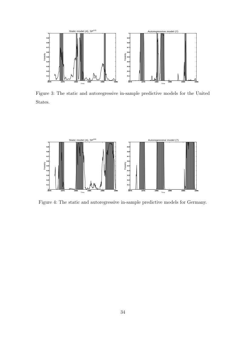
As an example of in-sample recession predictions, Figures 3 and 4 show the reces-

sion probabilities of the static model and the autoregressive model which are the first

and the fourth models in Tables 3 and 4. In out-of-sample forecasting, as discussed

in Section 3, the variable yt−1 is not observed at the time of forecasting t − h, when

h > 1. Therefore, we present the predictions of the in-sample models which are fully

comparable with the out-of-sample forecasts presented in the next section.

In the static model, the domestic term spread is the only predictive variable, but

in the autoregressive model all the experimented explanatory variables are included.

It can be seen that in the autoregressive model the recession probability matches

better the realized values of the recession indicator. A relatively high and positive

autoregressive coefficient for the πt−1 and employed additional explanatory variables

appears to be useful. In recession periods, the recession probabilities are also higher in

the autoregressive model. When the economy is in an expansionary state, the recession

probability is constantly higher in the static model whereas in the autoregressive

model it is very close to zero, as it should be.

4.3 Out-of-Sample Forecasting Results

The in-sample evidence shows a good deal of predictability for recession periods in the

U.S and Germany. However, in-sample predictability will not necessarily mean out-

of-sample predictability. For example, Estrella and Mishkin (1998) show that in the

case of the static probit model and U.S. recession periods, some of the best in-sample

predictive models perform quite poorly out-of-sample.

In this study, the first out-of-sample predictions are made for January 1995. The

sample period thus contains the recession period that began in both countries in 2001.

13

In other months, the economy is an expansionary state. If, for example, the forecast

horizon is 10 months, h = 10, then the values of the explanatory variables are known

up to 1994 M12 when the forecast for January 1995 is made. However, because of the

assumed nine-month publication lag in the recession indicator, the estimation period

is 1972 M1–1994 M2 (cf. Kauppi and Saikkonen, 2007). Further, the parameters in

the probit models are estimated recursively. After adding one month to the previous

estimation period and re-estimating the parameters, a forecast for the next month is

calculated. This procedure is repeated recursively until the end of the forecast sample.

The last out-of-sample forecasts are made for March 2007.

In out-of-sample forecasting results in Tables 5–8, the same forecasting models as

in the in-sample analysis are employed. Thus the variables included in the explanatory

variables vectors are

xUSt−k =

(

SP USt−6

, SP GEt−6

, rUSt−2

, rUSt−4

, rUSt−6

)

,

xGEt−k =

(

SP GEt−6

, SP USt−6

, rGEt−3

, rGEt−6

, rGEt−9

, ISt−6

)

,

where the lag orders are the same as the in-sample model selection suggested in the

previous section. The predictive models in which the foreign term spread is excluded

is also examined. In this case, the vectors of the explanatory variables are denoted

by xUS∗t−k and xGE∗

t−k . When the domestic term spread is the only predictor, then the

vectors are vUSt−k and vGE

t−k.9

When the forecast horizon h lengthens, the lags of explanatory variables should be

tailored so that only the information included in the information set Ωt−h at forecast

time t − h is used. For example, when the forecast horizon is 16 months meaning

that we are interested in forecasting the seven month (hf = 7) ahead value of the

recession indicator, then in the predictive models for the U.S., the vector xUSt−k contains

the following variables

xUSt−k =

(

SP USt−7

, SP GEt−7

, rUSt−7

)

.

Forecast accuracy is evaluated with the out-of-sample pseudo-R2 (Estrella, 1998).

In addition, the recession probabilities are also classified to construct different reces-

9 The lag orders of explanatory variables in these two cases are the same as above in xUSt−k and

xGEt−k.

14

sion signals. In this classification process, 50 and 25 percent thresholds are used to

classify the recession probabilities as ”strong”, ”weak” or ”no” recession signals. For

example, if the recession probability is between 25 and 50 percent, the model gives a

”weak” recession signal. In this classification the asymmetric forecasting point scheme

(cf. Dueker, 2002) presented in Table 2 is applied, which puts greater emphasis on

the right forecasts. It also prefers a false recession alarm compared to a missed reces-

sion month. The rationale behind this is that, for example, firms or policymakers are

willing to take a ”recession insurance” and accept a possible false alarm rather than

be caught by an unexpected recession.

Tables 5 and 6 show the out-of-sample forecasting performance of the employed

models in the U.S. As discussed in Section 3, the most interesting forecasts are for the

future values of the recession indicator. Therefore, the results from shorter horizons,

h ≤ 9, are available upon request. It is worth noting that in models where iterative

forecasts are considered, it is computationally too demanding to repeat the iterative

forecasts for the longest forecast horizon of 21 months.10 Therefore only the static

model (4) and the autoregressive model (7) are considered in those cases.

The best employed models yield accurate out-of-sample forecasts for the state of

the economy in the U.S. and, especially, for the beginning and the end of the recession

period starting in the year 2001. According to the values of the out-of-sample-psR2

and the forecasting points the highest predictive accuracy and the maximal forecast

horizon is obtained when the horizon is about 15 months, which is the same as hf = 6.

At this forecast horizon, the the autoregressive model (7) and the autoregressive

model with the interact term (8) outperform the iterative forecasts from the dynamic

model (5) yielding the best out-of-sample forecasts with the explanatory variables

included in the vector xUSt−k. In fact, the autoregressive interaction model is even the

best model when the forecast horizon is between 12 to 16 months, giving evidence

that there is asymmetric predictive content in the U.S. term spread depending on the

current state of the economy in out-of-sample forecasts as well.

The models with the U.S. stock returns (xUS∗t−k ) and the models with also a foreign

German term spread (xUSt−k) outperform the models with only the U.S. term spread

10 In iterative forecasts, it means that 221 different paths should be calculated before the forecast.

15

(vUSt−k) across all probit models and forecast horizons. Thus these additional financial

variables have predictive content also in the out-of-sample predictions for the U.S.

recessions.

Comparing the horizon-specific direct and iterative forecasts from the dynamic

model (5), the in-sample evidence that the iterative forecasting models based on the

yt−1 outperform the direct forecasts from the static or in the dynamic model with the

horizon-specific yt−h can be confirmed. In addition, as in Table 3, the autoregressive

coefficient α1 is in most cases statistically insignificant in the dynamic autoregressive

model (6). This model thus reduces to the dynamic model (5), and its out-of-sample

predictions are almost the same as in the dynamic model.11 Further, when the forecast

horizon is 21 months, which is the longest horizon considered, the static model turns

out to be an adequate model without any dynamics in the model equation. However,

in this forecast horizon also, the considered additional explanatory variables have

useful predictive power.

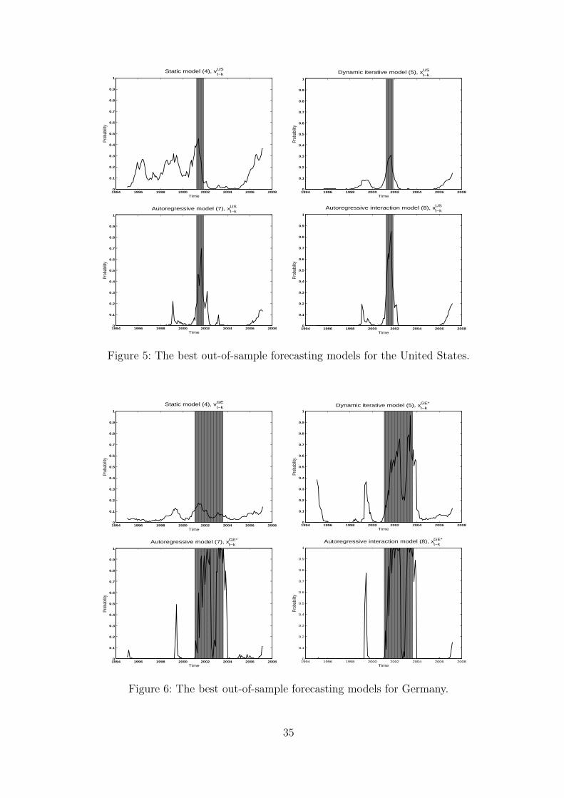
Figure 5 illustrates the out-of-sample performance of U.S. recession prediction

models when the forecast horizon is 15 months. These four models are highlighted in

Tables 5 and 6. The depicted forecasts indicate that the considered three dynamic

models certainly have the predictive power to forecast the beginning and the end

of the latest recession in 2001. The static model, where the U.S. term spread is

the single predictive variable, tends to produce significantly higher false recession

probability in the expansionary period compared with the dynamic models. In the

dynamic models the recession signals at the recession period are also more distinct

with higher recession probabilities. Kauppi and Saikkonen (2007) and Kauppi (2008)

stressed these same phenomena but, contrary to their findings, in this study the

autoregressive models (7) and (8) seem to generate somewhat better out-of-sample

forecasts compared with the iterative forecasts from the dynamic model (5). The

predictive power of the considered additional financial variables with the domestic

term spread is the main reason for this finding.

11 Therefore, Tables 5–6 only report the results from the dynamic iterative model (5). The same

is with the static model (4) which yield almost the same or even better predictions as the dynamic

direct model (cf. equation (13) with α1 = 0) since the coefficient for yt−h is statistically insignificant

for longer horizons h.

16

In the case of Germany, it is important to note that the latest recession period

lasted considerably longer than the recession in the U.S. as in Germany, the recession

ended in August 2003. Nevertheless, it can be seen that the essential conclusions

between different predictive models are parallel to predictive performance in the case

of the U.S. However, due to the fact that the term spreads rode up immediately after

the recession began (see Figure 1) it appears inevitable that the recession probability

would decrease midstream in the recession period. Thus the out-of-sample pseudo-R2

values are even negative in some models in Table 7. Therefore the forecasting points

in different models presented in Table 8 are the main model evaluation measure.

As in the U.S. it turns out that the dynamic iterative forecasts from the dynamic

model (5) are more accurate than the forecasts from the static model, and when the

forecast horizon increases towards 15 or 16 months the autoregressive models (7) and

(8) seem to outperform the alternative models. The evidence reflects that the interest

rate differential and German stock returns clearly have additional predictive power

also out-of-sample with the German term spread in all models (models with xGE∗

t−k ).

Interestingly, the U.S. term spread, which is a statistically significant predictor in-

sample, seems to be a quite poor predictive variable since the forecasting results are

much better without it. The statistical significance of the interest rate differential,

however, suggests that the U.S. monetary policy has an impact on the recession

probability in Germany via the short-term interest rate rUSt even though the U.S.

term spread is excluded from the predictive models.

It is interesting that the autoregressive interaction model (8) with the asymmetric

effects of the U.S. term spread SP USt seems to outperform the interaction model with

asymmetric effects on the German term spread when the explanatory variables in

vector xGEt−k are examined. Nevertheless, when the U.S. term spread is excluded from

the model, the asymmetric effect of the German term spread in the autoregressive in-

teraction model has, on average, only marginal additional predictive power compared

with the corresponding autoregressive model.

Figure 6 depicts the out-of-sample predictions of different models when the exa-

mined forecast horizon is 15 months. In the first, traditional static predictive model

with only the domestic German term spread, the recession probability is very low

17

during the recession period and the overall forecasting performance is quite disap-

pointing compared with the dynamic models with additional explanatory variables.

The recession probability indeed falls off during the recession period in all dynamic

models. However, the models manage to predict the start and the end of the recession

period quite well. As in the U.S. in the year 1999, the recession probability increased

but at that time there was no recession.

An other way to examine the likelihood of recession is obtained from the hitting

probabilities introduced by Chauvet and Potter (2005) and Kauppi and Saikkonen

(2007) who defined hitting probability of an economy being hit by a recession in

a particular month. In recession forecasting the probability of continued expansion,

which means a time period where the economy is in an expansionary state every

month, is particularly of interest. This is the complement probability of the cumulative

distribution where the hitting probabilities of individual months are calculated.

The evidence from the continued expansion probabilities of different expansio-

nary and recessionary periods is the same as above in month-to-month prediction.

The comparison between different models appears to depend on the state of the

economy. Using the static probit model, the recession probability appears to deviate

significantly from zero in expansionary periods, as seen for instance in Figures 5 and

6. In dynamic models the probabilities are more close to zero in expansionary periods.

Therefore during in expansionary periods the static model seems to overestimate the

probability of recession. On the other hand, in recession periods the dynamic model

(5) with iterative forecasts constantly gives the highest probabilities of continued

expansion. 12 Therefore, according to the continued expansion probabilities as well,

the autoregressive probit models (7) and (8) with domestic term spread and other

explanatory variables in a corresponding countries’ yield the best predictions.

4.4 Recession Probabilities in 2007 and 2008

Although the last and the future values of the recession indicator are unknown at the

end of the sample period, it is interesting to construct recession forecasts for those

months. In this section, we consider recession forecasts up to June 2008. Early in

12 Further details of continued expansion probabilities are available upon request.

18

2008, there was a great deal of uncertainty regarding the state of the U.S. economy.

The U.S. term spread has been low and even negative for quite a long time in 2007,

indicating a higher recession risk than at any time since the latest recession in 2001. At

the same time in Germany, it seems that the expansionary period is still continuing.

The estimated recession forecasts and corresponding continued expansion proba-

bilities at this 15-month time period are shown in Table 9. The forecast horizon is 15

months and thus the latest forecasts for June 2008 are based on the information from

December 2007. In the U.S., the recession probabilities are higher than 25 percent in

most of the latest months in all models. In the autoregressive interaction model the

forecast is higher than a 50 percent threshold value after August 2007.

In the case of Germany, the forecasts are quite high if the U.S. term spread is

included in the models. Nevertheless, as was found in the out-of-sample forecasts,

the forecasting power of the U.S. term spread in Germany is questionable. If it is

withdrawn from the forecasting models, then the probability forecasts are clearly

lower than with it. The best out-of-sample dynamic models proposed in the previ-

ous section, in which the U.S. term spread is excluded, indicate that the recession

probabilities are increasing in the latest months considered.

On the whole, the recession risk appears to be higher than at any time since the

last recession in both countries.

5 Conclusions

This paper has examined the performance of recession prediction models which are

based on the dynamic probit models and a number of financial explanatory variables.

Following the evidence in previous studies, the term spread is found a useful predic-

tive variable for the U.S. and German recessions. However, according to the results

presented here, stock market returns have additional predictive power to forecast

recession periods in both countries using different probit models and the predictive

information is distributed in many lagged stock returns. The short-term interest rate

differential between the United States and Germany also has substantial predictive

content in terms of both in-sample and out-of-sample predictions to predict German

19

recession. The same is true with the foreign German term spread in forecasting the

U.S. recessions. In addition the U.S. term spread is also a statistically significant

predictor in the case of Germany but its out-of-sample predictive content appears to

be poor in the last recession period.

Based on the comparisons between different probit models, the results indicate

that statistically significant additional predictive content is obtained by allowing for

dynamic structures in the predictive model compared with the traditional static model

used in many previous studies. Especially, the probit models with statistically sig-

nificant autoregressive structure in model equation performed somewhat better out-

of-sample than the static and other dynamic models. Especially, the experimented

autoregressive interaction model where the U.S. term spread have an asymmetric ef-

fect on recession probability depending the state of the economy, provide accurate

forecasts for the recession periods in the U.S and Germany.

References

Akaike, H. (1974): A new look at statistical model identification. IEEE Transactions

on Automatic Control, 19, 713–723.

Bernard, H., and Gerlach, S. (1998): Does the term structure predict recessions? The

international evidence. International Journal of Finance and Economics, 3, 195–215.

Boulier, B. L., and Steckler, H. O. (2000): The term spread as a monthly cyclical

indicator. Economics Letters, 66, 79–83.

Chauvet, M., and Potter, S. (2005): Forecasting recession using the yield curve. Jour-

nal of Forecasting, 24(2), 77–103.

Davis, E. P., and Fagan, G. (1997): Are financial spreads useful indicators of future

inflation and output growth in EU countries? Journal of Applied Econometrics, 12,

701–714.

20

de Jong, R. M., and Woutersen, T. M. (2007): Dynamic time series binary choice.

Economics Working Paper Archive, 538. The Johns Hopkins University, Department

of Economics. Available at http://www.econ.jhu.edu/pdf/papers/WP538.pdf.

Diebold, F. X., and Rudebusch, G. D. (1989): Scoring the leading indicators. Journal

of Business, 62(3), 369–391.

Dueker, M. J. (1997): Strengthening the case for the yield curve as a predictor of U.S.

recessions. Federal Reserve Bank of St.Louis Review, 79, 41–51.

Dueker, M. J. (2002): Regime-dependent recession forecasts and the 2001 recession.

Federal Reserve Bank of St.Louis Review, 84, 29–36.

Dueker, M. J. (2005): Dynamic forecasts of qualitative variables: A qual VAR model

of U.S. recessions. Journal of Business and Economic Statistics, 23(1), 96–104.

Estrella, A. (1998): A new measure of fit for equations with dichotomous dependent

variables. Journal of Business and Economic Statistics, 16, 198–205.

Estrella, A. (2005a): The yield curve as a leading indicator: Frequently asked ques-

tions. Federal Reserve Bank of New York. Available at http:/www.newyorkfed.org/research/

capital_markets/ycfaq.pdf.

Estrella, A. (2005b): Why does the yield curve predict output and inflation? The

Economic Journal, 115, 722–744.

Estrella, A., and Hardouvelis, G. A. (1991): The term structure as a predictor of real

economic activity. Journal of Finance, 46, 555–576.

21

Estrella, A., and Mishkin, F. S. (1998): Predicting U.S. recessions: Financial variables

as leading indicators. Review of Economics and Statistics, 80(1), 45–61.

Estrella, A., and Rodrigues, A. P. (1998): Consistent covariance matrix estimation in

probit models with autocorrelated disturbances. Federal Reserve Bank of New York

Staff Reports, 39.

Estrella, A., Rodrigues, A. P., and Schich, S. (2003): How stable is the predictive

power of the yield curve: Evidence from Germany and the United States. Review of

Economics and Statistics, 85, 629–644.

Fama, E. F. (1990): Stock returns, expected returns, and real activity. Journal of

Finance, 45, 1089–1108.

Florio, A. (2004): The asymmetric effects of monetary policy. Journal of Economic

Surveys, 84(2), 409–426.

Kauppi, H. (2008): Yield-Curve Based Probit Models for Forecasting U.S. Recessions:

Stability and Dynamics. HECER Discussion Paper, 221. Helsinki Center of Economic

Research.

Kauppi, H., and Saikkonen, P. (2007): Predicting U.S. recessions with dynamic bi-

nary response models. Review of Economics and Statistics, forthcoming.

Marcellino, M. , Stock J. H., and Watson, M. W. (2006): A comparison of direct and

iterated AR methods for forecasting macroeconomic time series. Journal of Econo-

metrics, 135, 499-526.

Moneta, F. (2003): Does the yield spread predict recessions in the Euro area? ECB

working paper, 294.

22

Morgan, D. P. (1993): Asymmetric effects of monetary policy. Federal Reserve Bank

of Kansas City Economic Review, 21–33.

Romer, D. (2001): Advanced Macroeconomics. Second edition. McGraw-Hill, New

York.

Rydberg, T., and Shephard, N. (2003): Dynamics of trade-by-trade price movements:

Decomposition and models. Journal of Financial Econometrics, 1, 2–25.

Schwarz, G. (1978): Estimating the dimension of a model. Annals of Statistics, 6,

461–464.

Stock, J. H., and Watson, M. W. (2003): Forecasting output and inflation: The role

of asset prices. Journal of Economic Literature, 41, 788–829.

Valckx, N., de Ceuster, M. J. K., and Annaert, J. (2002): Is financial market volatility

informative to predict recessions? DNB Staff Report, 93.

Wright, J. H. (2006): The yield curve and predicting recessions. Finance and Eco-

nomics Discussion Series, 2006-2007. Board of Governors of the Federal Reserve Sys-

tem.

23

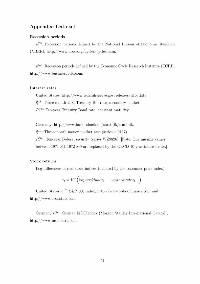
Appendix: Data set

Recession periods

yUSt : Recession periods defined by the National Bureau of Economic Research

(NBER), http://www.nber.org/cycles/cyclesmain.

yGEt : Recession periods defined by the Economic Cycle Research Institute (ECRI),

http://www.businesscycle.com.

Interest rates

United States: http://www.federalreserve.gov/releases/h15/data.

iUSt : Three-month U.S. Treasury Bill rate, secondary market.

RUSt : Ten-year Treasury Bond rate, constant maturity.

Germany: http://www.bundesbank.de/statistik/statistik.

iGEt : Three-month money market rate (series su0107).

RGEt : Ten-year Federal security (series WZ9826). [Note: The missing values

between 1971 M1-1972 M9 are replaced by the OECD 10-year interest rate.]

Stock returns

Log-differences of real stock indices (deflated by the consumer price index)

rt = 100(

log stockindext − log stockindext−1

)

.

United States rUSt : S&P 500 index, http://www.yahoo.finance.com and

http://www.econstats.com.

Germany rGEt : German MSCI index (Morgan Stanley International Capital),

http://www.mscibarra.com.

24

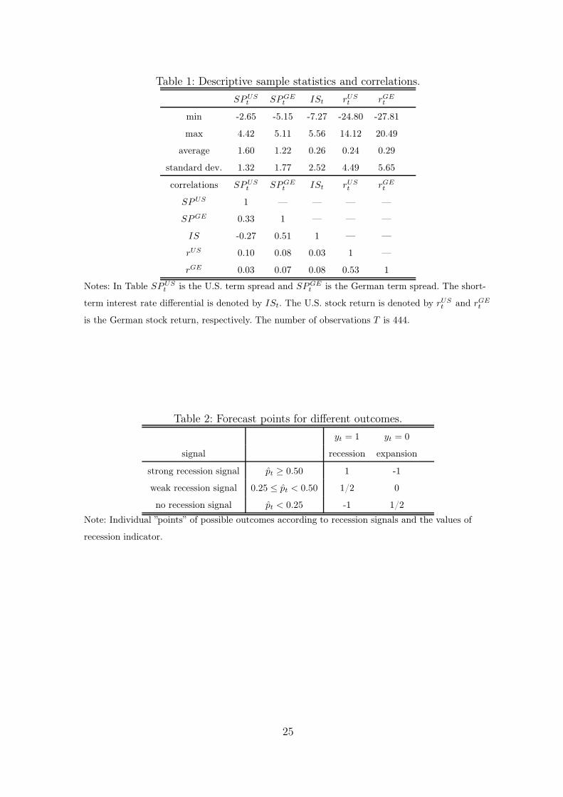
Table 1: Descriptive sample statistics and correlations.

SPUSt SPGE

t ISt rUSt rGE

t

min -2.65 -5.15 -7.27 -24.80 -27.81

max 4.42 5.11 5.56 14.12 20.49

average 1.60 1.22 0.26 0.24 0.29

standard dev. 1.32 1.77 2.52 4.49 5.65

correlations SPUSt SPGE

t ISt rUSt rGE

t

SPUS 1 — — — —

SPGE 0.33 1 — — —

IS -0.27 0.51 1 — —

rUS 0.10 0.08 0.03 1 —

rGE 0.03 0.07 0.08 0.53 1

Notes: In Table SPUSt is the U.S. term spread and SPGE

t is the German term spread. The short-

term interest rate differential is denoted by ISt. The U.S. stock return is denoted by rUSt and rGE

t

is the German stock return, respectively. The number of observations T is 444.

Table 2: Forecast points for different outcomes.

yt = 1 yt = 0

signal recession expansion

strong recession signal pt ≥ 0.50 1 -1

weak recession signal 0.25 ≤ pt < 0.50 1/2 0

no recession signal pt < 0.25 -1 1/2

Note: Individual ”points” of possible outcomes according to recession signals and the values of

recession indicator.

25

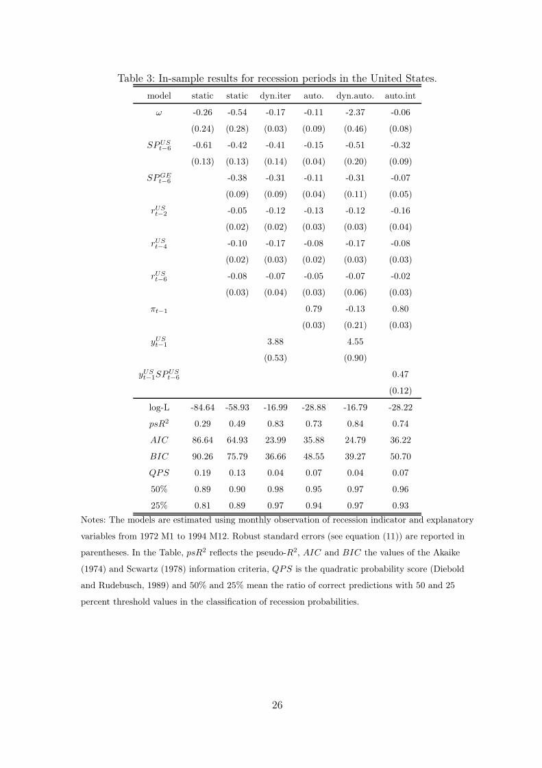
Table 3: In-sample results for recession periods in the United States.

model static static dyn.iter auto. dyn.auto. auto.int

ω -0.26 -0.54 -0.17 -0.11 -2.37 -0.06

(0.24) (0.28) (0.03) (0.09) (0.46) (0.08)

SPUSt−6

-0.61 -0.42 -0.41 -0.15 -0.51 -0.32

(0.13) (0.13) (0.14) (0.04) (0.20) (0.09)

SPGEt−6

-0.38 -0.31 -0.11 -0.31 -0.07

(0.09) (0.09) (0.04) (0.11) (0.05)

rUSt−2

-0.05 -0.12 -0.13 -0.12 -0.16

(0.02) (0.02) (0.03) (0.03) (0.04)

rUSt−4

-0.10 -0.17 -0.08 -0.17 -0.08

(0.02) (0.03) (0.02) (0.03) (0.03)

rUSt−6 -0.08 -0.07 -0.05 -0.07 -0.02

(0.03) (0.04) (0.03) (0.06) (0.03)

πt−1 0.79 -0.13 0.80

(0.03) (0.21) (0.03)

yUSt−1 3.88 4.55

(0.53) (0.90)

yUSt−1

SPUSt−6

0.47

(0.12)

log-L -84.64 -58.93 -16.99 -28.88 -16.79 -28.22

psR2 0.29 0.49 0.83 0.73 0.84 0.74

AIC 86.64 64.93 23.99 35.88 24.79 36.22

BIC 90.26 75.79 36.66 48.55 39.27 50.70

QPS 0.19 0.13 0.04 0.07 0.04 0.07

50% 0.89 0.90 0.98 0.95 0.97 0.96

25% 0.81 0.89 0.97 0.94 0.97 0.93

Notes: The models are estimated using monthly observation of recession indicator and explanatory

variables from 1972 M1 to 1994 M12. Robust standard errors (see equation (11)) are reported in

parentheses. In the Table, psR2 reflects the pseudo-R2, AIC and BIC the values of the Akaike

(1974) and Scwartz (1978) information criteria, QPS is the quadratic probability score (Diebold

and Rudebusch, 1989) and 50% and 25% mean the ratio of correct predictions with 50 and 25

percent threshold values in the classification of recession probabilities.

26

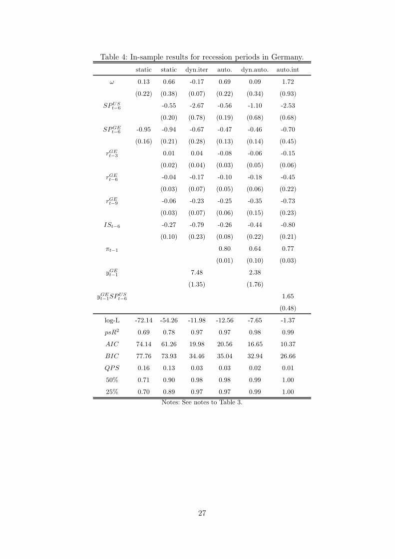
Table 4: In-sample results for recession periods in Germany.

static static dyn.iter auto. dyn.auto. auto.int

ω 0.13 0.66 -0.17 0.69 0.09 1.72

(0.22) (0.38) (0.07) (0.22) (0.34) (0.93)

SPUSt−6

-0.55 -2.67 -0.56 -1.10 -2.53

(0.20) (0.78) (0.19) (0.68) (0.68)

SPGEt−6

-0.95 -0.94 -0.67 -0.47 -0.46 -0.70

(0.16) (0.21) (0.28) (0.13) (0.14) (0.45)

rGEt−3

0.01 0.04 -0.08 -0.06 -0.15

(0.02) (0.04) (0.03) (0.05) (0.06)

rGEt−6

-0.04 -0.17 -0.10 -0.18 -0.45

(0.03) (0.07) (0.05) (0.06) (0.22)

rGEt−9 -0.06 -0.23 -0.25 -0.35 -0.73

(0.03) (0.07) (0.06) (0.15) (0.23)

ISt−6 -0.27 -0.79 -0.26 -0.44 -0.80

(0.10) (0.23) (0.08) (0.22) (0.21)

πt−1 0.80 0.64 0.77

(0.01) (0.10) (0.03)

yGEt−1

7.48 2.38

(1.35) (1.76)

yGEt−1

SPUSt−6

1.65

(0.48)

log-L -72.14 -54.26 -11.98 -12.56 -7.65 -1.37

psR2 0.69 0.78 0.97 0.97 0.98 0.99

AIC 74.14 61.26 19.98 20.56 16.65 10.37

BIC 77.76 73.93 34.46 35.04 32.94 26.66

QPS 0.16 0.13 0.03 0.03 0.02 0.01

50% 0.71 0.90 0.98 0.98 0.99 1.00

25% 0.70 0.89 0.97 0.97 0.99 1.00

Notes: See notes to Table 3.

27

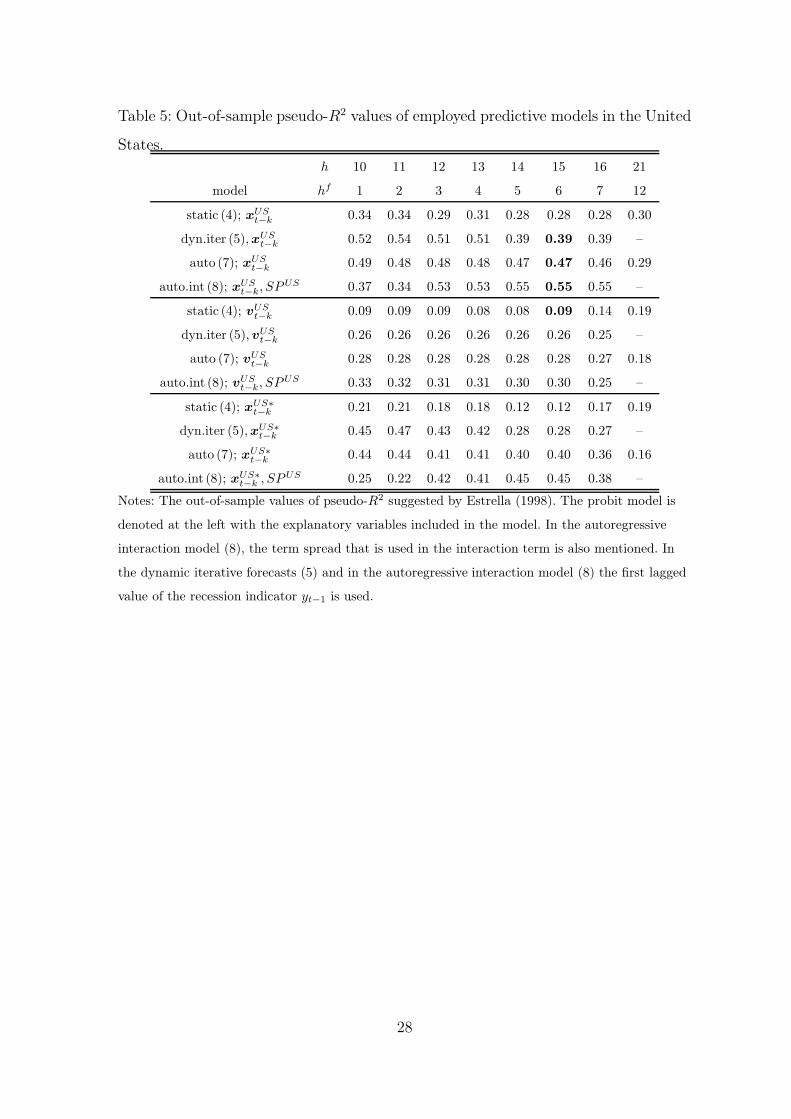
Table 5: Out-of-sample pseudo-R2 values of employed predictive models in the United

States.

h 10 11 12 13 14 15 16 21

model hf 1 2 3 4 5 6 7 12

static (4); xUSt−k 0.34 0.34 0.29 0.31 0.28 0.28 0.28 0.30

dyn.iter (5), xUSt−k 0.52 0.54 0.51 0.51 0.39 0.39 0.39 –

auto (7); xUSt−k 0.49 0.48 0.48 0.48 0.47 0.47 0.46 0.29

auto.int (8); xUSt−k, SPUS 0.37 0.34 0.53 0.53 0.55 0.55 0.55 –

static (4); vUSt−k 0.09 0.09 0.09 0.08 0.08 0.09 0.14 0.19

dyn.iter (5), vUSt−k 0.26 0.26 0.26 0.26 0.26 0.26 0.25 –

auto (7); vUSt−k 0.28 0.28 0.28 0.28 0.28 0.28 0.27 0.18

auto.int (8); vUSt−k, SPUS 0.33 0.32 0.31 0.31 0.30 0.30 0.25 –

static (4); xUS∗

t−k 0.21 0.21 0.18 0.18 0.12 0.12 0.17 0.19

dyn.iter (5), xUS∗

t−k 0.45 0.47 0.43 0.42 0.28 0.28 0.27 –

auto (7); xUS∗

t−k 0.44 0.44 0.41 0.41 0.40 0.40 0.36 0.16

auto.int (8); xUS∗

t−k , SPUS 0.25 0.22 0.42 0.41 0.45 0.45 0.38 –

Notes: The out-of-sample values of pseudo-R2 suggested by Estrella (1998). The probit model is

denoted at the left with the explanatory variables included in the model. In the autoregressive

interaction model (8), the term spread that is used in the interaction term is also mentioned. In

the dynamic iterative forecasts (5) and in the autoregressive interaction model (8) the first lagged

value of the recession indicator yt−1 is used.

28

Table 6: Out-of-sample forecasting points of employed predictive models in the United

States.

h 10 11 12 13 14 15 16 21

model hf 1 2 3 4 5 6 7 12

static (4); xUSt−k 0.82 0.82 0.82 0.78 0.82 0.82 0.82 0.78

dyn.iter (5), xUSt−k 0.86 0.87 0.88 0.88 0.81 0.81 0.81 –

auto (7); xUSt−k 0.84 0.84 0.85 0.85 0.85 0.85 0.85 0.78

auto.int (8); xUSt−k, SPUS 0.84 0.83 0.87 0.87 0.91 0.91 0.90 –

static (4); vUSt−k 0.67 0.67 0.67 0.66 0.66 0.67 0.70 0.76

dyn.iter (5), vUSt−k 0.82 0.82 0.82 0.82 0.83 0.82 0.82 –

auto (7); vUSt−k 0.80 0.80 0.80 0.80 0.80 0.80 0.79 0.71

auto.int (8); vUSt−k, SPUS 0.79 0.78 0.77 0.77 0.76 0.76 0.73 –

static (4); xUS∗

t−k 0.79 0.79 0.77 0.77 0.75 0.75 0.78 0.75

dyn.iter (5), xUS∗

t−k 0.84 0.84 0.86 0.86 0.85 0.85 0.84 –

auto (7); xUS∗

t−k 0.82 0.82 0.82 0.82 0.85 0.85 0.85 0.68

auto.int (8); xUS∗

t−k , SPUS 0.83 0.83 0.85 0.83 0.85 0.85 0.80 –

Notes: Forecasting points are obtained from the point scheme presented in Table 2 by dividing the

sum of individual points by the number of maximum points which means that the state of the

economy is predicted correctly in every month.

29

Table 7: The out-of-sample values of psR2 of employed models in Germany.

h 10 11 12 13 14 15 16 21

model hf 1 2 3 4 5 6 7 12

static (4); xGEt−k 0.07 0.03 0.00 neg neg neg neg 0.14

dyn.iter (5), xGEt−k neg neg neg neg neg neg neg –

auto (7); xGEt−k 0.35 0.36 0.37 neg neg 0.02 neg 0.16

auto.int (8); xGEt−k, SPUS neg neg neg neg neg neg neg –

auto.int (8); xGEt−k, SPGE neg neg neg neg neg neg neg –

static (4); vGEt−k 0.02 0.02 0.02 0.02 0.02 0.02 0.16 0.03

dyn.iter (5), vGEt−k 0.44 0.41 0.38 0.36 0.34 0.32 0.30 –

auto (7); vGEt−k 0.20 0.20 0.19 0.19 0.19 0.19 0.19 0.27

auto.int (8); vGEt−k, SPGE neg neg neg neg neg. neg 0.11 –

static (4); xGE∗

t−k 0.41 0.40 0.38 0.38 0.38 0.38 0.35 0.28

dyn.iter (5), xGE∗

t−k 0.61 0.60 0.58 0.60 0.60 0.59 0.41 –

auto (7); xGE∗

t−k 0.70 0.70 0.69 0.57 0.58 0.59 0.57 0.27

auto.int (8); xGE∗

t−k , SPGE neg. neg. neg. 0.49 0.51 0.52 0.57 –

Notes: ”Neg” means negative psR2-value. See also notes to Table 5.

30

Table 8: Out-of-sample forecasting points of employed models in Germany.

h 10 11 12 13 14 15 16 21

model hf 1 2 3 4 5 6 7 12

static (4); xGEt−k 0.53 0.49 0.49 0.50 0.48 0.50 0.48 0.50

dyn.iter (5), xGEt−k 0.66 0.64 0.63 0.61 0.60 0.60 0.55 –

auto (7); xGEt−k 0.74 0.74 0.74 0.73 0.73 0.70 0.71 0.52

auto.int (8); xGEt−k, SPUS 0.65 0.63 0.60 0.60 0.60 0.60 0.49 –

auto.int (8); xGEt−k, SPGE 0.60 0.52 0.52 0.50 0.50 0.48 0.45 –

static (4); vGEt−k 0.29 0.29 0.29 0.30 0.29 0.30 0.41 0.30

dyn.iter (5), vGEt−k 0.56 0.55 0.52 0.48 0.49 0.48 0.43 –

auto (7); vGEt−k 0.44 0.44 0.44 0.44 0.42 0.42 0.41 0.42

auto.int (8); vGEt−k, SPGE 0.52 0.52 0.52 0.52 0.52 0.52 0.50 –

static (4); xGE∗

t−k 0.60 0.58 0.58 0.58 0.58 0.58 0.58 0.53

dyn.iter (5), xGE∗

t−k 0.72 0.71 0.67 0.69 0.67 0.67 0.61 –

auto (7); xGE∗

t−k 0.81 0.81 0.81 0.71 0.71 0.71 0.70 0.53

auto.int (8); xGE∗

t−k , SPGE 0.66 0.67 0.62 0.75 0.75 0.75 0.70 –

Notes: See notes to Table 6.

31

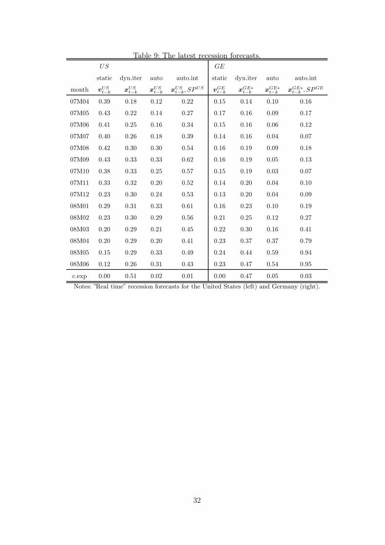
Table 9: The latest recession forecasts.

US GE

static dyn.iter auto auto.int static dyn.iter auto auto.int

month vUSt−k xUS

t−k xUSt−k xUS

t−k, SPUS vGEt−k xGE∗

t−k xGE∗

t−k xGE∗

t−k , SPGE

07M04 0.39 0.18 0.12 0.22 0.15 0.14 0.10 0.16

07M05 0.43 0.22 0.14 0.27 0.17 0.16 0.09 0.17

07M06 0.41 0.25 0.16 0.34 0.15 0.16 0.06 0.12

07M07 0.40 0.26 0.18 0.39 0.14 0.16 0.04 0.07

07M08 0.42 0.30 0.30 0.54 0.16 0.19 0.09 0.18

07M09 0.43 0.33 0.33 0.62 0.16 0.19 0.05 0.13

07M10 0.38 0.33 0.25 0.57 0.15 0.19 0.03 0.07

07M11 0.33 0.32 0.20 0.52 0.14 0.20 0.04 0.10

07M12 0.23 0.30 0.24 0.53 0.13 0.20 0.04 0.09

08M01 0.29 0.31 0.33 0.61 0.16 0.23 0.10 0.19

08M02 0.23 0.30 0.29 0.56 0.21 0.25 0.12 0.27

08M03 0.20 0.29 0.21 0.45 0.22 0.30 0.16 0.41

08M04 0.20 0.29 0.20 0.41 0.23 0.37 0.37 0.79

08M05 0.15 0.29 0.33 0.49 0.24 0.44 0.59 0.94

08M06 0.12 0.26 0.31 0.43 0.23 0.47 0.54 0.95

c.exp 0.00 0.51 0.02 0.01 0.00 0.47 0.05 0.03

Notes: ”Real time” recession forecasts for the United States (left) and Germany (right).

32

1970 1975 1980 1985 1990 1995 2000 2005 2010Time

US

1970 1975 1980 1985 1990 1995 2000 2005 2010−8

−6

−4

−2

0

2

4

6

SPUS

IS

1970 1975 1980 1985 1990 1995 2000 2005 2010Time

GE

1970 1975 1980 1985 1990 1995 2000 2005 2010−8

−6

−4

−2

0

2

4

6

SPGE

IS

Figure 1: Recession periods with domestic term spread SPt and the interest rate dif-

ferential ISt. The United States (SP USt ) is shown in the left panel, Germany (SP GE

t )

in the right panel.

1970 1975 1980 1985 1990 1995 2000 2005 2010

Time

US

1970 1975 1980 1985 1990 1995 2000 2005 2010−25

−20

−15

−10

−5

0

5

10

15

1970 1975 1980 1985 1990 1995 2000 2005 2010

GE

Time1970 1975 1980 1985 1990 1995 2000 2005 2010

−30

−20

−10

0

10

20

30

Figure 2: Recession periods with stock returns rt. The United States (rUSt ) is shown

in the left panel, Germany (rGEt ) in the right panel.

33

1970 1975 1980 1985 1990 19950

0.1

0.2

0.3

0.4

0.5

0.6

0.7

0.8

0.9

1

Time

Prob

abilit

y

Static model (4), SPUS

1970 1975 1980 1985 1990 19950

0.1

0.2

0.3

0.4

0.5

0.6

0.7

0.8

0.9

1

1970 1975 1980 1985 1990 19950

0.1

0.2

0.3

0.4

0.5

0.6

0.7

0.8

0.9

1

Time

Prob

abilit

y

Autoregressive model (7)

1970 1975 1980 1985 1990 19950

0.1

0.2

0.3

0.4

0.5

0.6

0.7

0.8

0.9

1

Figure 3: The static and autoregressive in-sample predictive models for the United

States.

1970 1975 1980 1985 1990 19950

0.1

0.2

0.3

0.4

0.5

0.6

0.7

0.8

0.9

1

Time

Prob

abilit

y

Static model (4), SPGE

1970 1975 1980 1985 1990 19950

0.1

0.2

0.3

0.4

0.5

0.6

0.7

0.8

0.9

1

1970 1975 1980 1985 1990 19950

0.1

0.2

0.3

0.4

0.5

0.6

0.7

0.8

0.9

1

Time

Prob

abilit

y

Autoregressive model (7)

1970 1975 1980 1985 1990 19950

0.1

0.2

0.3

0.4

0.5

0.6

0.7

0.8

0.9

1

Figure 4: The static and autoregressive in-sample predictive models for Germany.

34

1994 1996 1998 2000 2002 2004 2006 20080

0.1

0.2

0.3

0.4

0.5

0.6

0.7

0.8

0.9

1

Time

Prob

abilit

y

Static model (4), vt−kUS

1994 1996 1998 2000 2002 2004 2006 20080

0.1

0.2

0.3

0.4

0.5

0.6

0.7

0.8

0.9

1

Time

Prob

abilit

y

Dynamic iterative model (5), xt−kUS

1994 1996 1998 2000 2002 2004 2006 20080

0.1

0.2

0.3

0.4

0.5

0.6

0.7

0.8

0.9

1

Time

Prob

abilit

y

Autoregressive model (7), xt−kUS

1994 1996 1998 2000 2002 2004 2006 20080

0.1

0.2

0.3

0.4

0.5

0.6

0.7

0.8

0.9

1

Time

Prob

abilit

y

Autoregressive interaction model (8), xt−kUS

Figure 5: The best out-of-sample forecasting models for the United States.

1994 1996 1998 2000 2002 2004 2006 20080

0.1

0.2

0.3

0.4

0.5

0.6

0.7

0.8

0.9

1

Time

Prob

abilit

y

Static model (4), vt−kGE

1994 1996 1998 2000 2002 2004 2006 20080

0.1

0.2

0.3

0.4

0.5

0.6

0.7

0.8

0.9

1

Time

Prob

abilit

y

Dynamic iterative model (5), xt−kGE*

1994 1996 1998 2000 2002 2004 2006 20080

0.1

0.2

0.3

0.4

0.5

0.6

0.7

0.8

0.9

1

Time

Prob

abilit

y

Autoregressive model (7), xt−kGE*

1994 1996 1998 2000 2002 2004 2006 20080

0.1

0.2

0.3

0.4

0.5

0.6

0.7

0.8

0.9

1

Time

Prob

abilit

y

Autoregressive interaction model (8), xt−kGE*

Figure 6: The best out-of-sample forecasting models for Germany.

35